The hyperbolic class of quadratic time-frequency ... · The Hyperbolic Class of Quadratic Time-Frequency ... on the analysis time or analysis frequency ... achieved by the short-time

IEEE TRANSACTIONS O N SIGNAL PROCESSING VOL 41 NO 12 DECEMBER 1993 3425

The Hyperbolic Class of Quadratic Time-Frequency Representations Part I: Constant-Q Warping, the Hyperbolic Paradigm, Properties, and Members

Antonia Papandreou, Student Member, IEEE, Franz Hlawatsch, Member, IEEE, and G . Faye Boudreaux-Bartels, Member, IEEE

Abstract-The time-frequency (TF) version of the wavelet transform and the “affine” quadraticlbilinear TF representations can be used for a TF analysis with constant-Q characteristic. This paper considers a new approach to constant-Q TF analysis. A specific TF warping transform is applied to Cohen’s class of quadratic TF representations, which results in a new class of quadratic TF representations with constant-Q characteristic. The new class is related to a “hyperbolic TF geometry” and is thus called the hyperbolic class (HC). Two prominent TF representations previously considered in the literature, the Bertrand Po distribution and the Altes-Marinovic Q-distribution, are members of the new HC. We show that any hyperbolic TF representation is related to both the wideband ambiguity function and a “hyperbolic ambiguity function.” It is also shown that the HC is the class of all quadratic TF representations which are invariant to “hyperbolic time-shifts” and TF scalings, operations which are important in the analysis of Doppler-invariant signals and self-similar random processes.

The paper discusses the definition of the HC via constant-Q warping, some signal-theoretic fundamentals of the “hyperbolic TF geometry,’’ and the description of the HC by 2-D kernel functions. Several members of the HC are considered, and a list of desirable properties of hyperbolic TF representations is given together with the associated kernel constraints.

I. INTRODUCTION

UADRATIC time-frequency representations (QTFR’s) are useful in the analysis of nonstationary

signals [l]. This paper discusses a new class of “constant-Q” QTFR’s. By way of introduction, and to establish the notation used, we first give a brief review of two basic QTFR classes. In the following, let x ( t ) be a signal with Fourier transform X( f ) = jYm x(t)e-’2*fr dt.

Q

Manuscript received September 8, 1992; revised May 5, 1993. The Guest Editor coordinating the review of this paper and approving it for publica- tion was Dr. Patrick Flandrin. This work was supported in part by Office of Naval Research under Grants N00014-89-J-1812 and N00014-92-J-1499 and in part by the Fonds zur Forderung der wisaenschaftlichen Forschung under Grants P7354-PHY and J0530-TEC.

A . Papandreou and G . F. Boudreaux-Bartels are with the Department of Electrical Engineering. University of Rhode Island. Kingston, RI 02881.

F. Hlawatsch is with INTHFT, Technische Universitiit Wien, Gusshaus- strasse 251389, A- 1040 Vienna, Austria.

IEEE Log Number 92 12 182.

A . Cohen ’s Class and Constant-Bandwidth Time- Frequency Analysis

Many important QTFR’s are members of Cohen ’s class with signal independent kernels’ [ 11-[4] which contains all QTFR’s T(”(t, f ) satisfying the time-shift and frequency-shift invariance properties*

Here, the time-shift operator S, and the frequency-shift operator Xu are defined by (S,X)(f) = e - j Z T r f X ( f ) and (nZ,X)(f) = X ( f - v), respectively. It is well known that any QTFR of Cohen’s class can be written as3

T F k f 1

r m r m

- $;=I (t - t ’, f - f ’ ) W x ( t ’ , f’) dt ’ df’ (4) - b m I,

‘Hereafter referred to as Cohen’s class for simplicity. ’Note that. for example, Ti:i(r. f ) stands for T?’( t . f ) with Y ( f ) =

For the sake of notational simplicity, we shall usually consider quadratic auto-representations TkcF’(t, f ) only. The extension to bilinear cross- representations T:, b(f, f ) is straightforward, e.g., TkCb(r, f ) = jrm jrm $:“(I - r ‘, r )ux Y ( t ‘, r)e-’’=” dt ’ dr with I A ~ , ~ ( ~ ? r ) = x ( t + r/2).v*(t - r /2) . Also, since most signal transforms relevant to our discussion are best formulated in the frequency domain, we shall typically denote signals by their Fourier transforms, e.g., we write T F ’ ( t , f ) rather than T ; “ ( t , f ) .

( S ; X ) ( f ).

1053-587X/93$03.00 0 1993 IEEE

Copyright IEEE 1993

3426 IEEE TRANSACTIONS ON SIGNAL PROCESSING. VOL. 41. NO. 12, DECEMBER 1993

with the “signal products” The squared magnitude of the wavelet transform (known as the scalogram) [6] can be written in terms of the WD as ux( t , 7) . ( t + ; ) . * ( I - ;),

SCALx(t, f ) = lWTx(f, f > I2 U,(f , v) = X(f + ;) X * ( f - ;), m m

= j-m W r ( i ( f ‘ - o,L’) f the Wigner distribution (WD)

. Wx(t ‘, f ’) dt ’ df ’ (8) Wx( t , f ) = im ux( t , r)e-jZTfr dr

-m where I’ ( f ) is the Fourier transform of the wavelet y ( t ) . m Hence, the scalogram is a smooth WD, for which the

= 5 U,( f, v)eJ2Tr” dv, amounts of frequency and time smoothing are propor- -m tional and inversely proportional, respectively, to the

analysis frequency f. This type of “affine smoothing” re- and the (narrowband) ambiguity function (AF) sults in a constant-Q TF analysis.

The aflne class of QTFR’s [6]-[9] is obtained by gen- eralizing (8) as AX(7, v) = jm -m ux(t , 7)e-J2*”f dt

The “kernels” +$‘)(t, T), +$“(f, v), $$“(t, f), and \k‘,‘’(~, v) are interrelated by Fourier transforms in exactly the same way as are the corresponding quadratic signal representations ux( t , T ) , U,( f, v), Wx(t , f ) , andAx(7, v) 141. Any of the four kernels uniquely characterizes the QTFR T“’.

The time-frequency (TF) shift invariance property (1) underlying Cohen’s class implies a type of TF analysis where the QTFR’s analysis characteristics do not change with time t and frequency f. In particular, all TF points ( t , f) are analyzed with the same time resolution and the same frequency resolution. This is similar to the constant- bandwidth analysis achieved by the short-time Fourier transform, where the analysis bandwidth does not depend on the analysis time or analysis frequency. In fact, the squared magnitude of the short-time Fourier transform (known as the spectrogram) is a member of Cohen’s class 111, 131.

B. The Aflne Class and Constant-Q Time-Frequency Analysis

An alternative to the constant-bandwidth analysis achieved by the short-time Fourier transform and QTFR’s of Cohen’s class is provided by the wavelet transform and the afine class of QTFR’s.

The TF version of the wavelet transform (WT) is a linear TF representation defined as [l] , [5]

where the analysis wavelet y ( t ) is a bandpass function with center frequency f r . For the wavelet transform, the analysis bandwidth is proportional to the analysis frequency f, i.e., the quality factor Q = center frequency t bandwidth is independent of the analysis frequency (‘ ‘constant-Q analysis”).

Wx(t ’, f ’) dr ‘ df ’ (9) where $y’(a, 0) is a two-dimensional kernel function. If this kernel is a sufficiently smoothed function concentrated about 0 = 1, then (9) results in an affine smoothing of the WD, just as in the case of the scalogram in (8). The affine QTFR class can alternatively be defined as the class of all QTFR’s that are invariant to time-shifts and TF scalings, i.e.,

T & ( t , f ) = TY’(t - 7 , f ) ,

with the time-shift operator S, as before and the TF scaling operator e, defined as

The TF scaling operator e, is a unitary, linear operator which produces a frequency scaling (simultaneously an inverse time scaling). This scaling transform is of basic importance in multiscale or multiresolution analysis (by means of the wavelet transform or affine QTFR’s [5], [6], [SI), for self-similar signals [lo], scale-invariant systems [ l l ] , and in the context of the (wideband) Doppler effect 1121.

An alternative approach to constant-Q analysis has been proposed by Altes in [ 131. A specific T F warping is used to convert the WD into a “wideband WD” called the Q-distribution. This approach, which is also closely connected with the TF scaling operator e,, will be further considered in Section 11.

C. The Hyperbolic Geometry The scaling operator e, is intimately related to a “hy-

perbolic TF geometry” [7]-[lo], [13]-1181. First, con-

PAPANDREOU er u l . . THF. HYPERBOLIC CLASS 3421

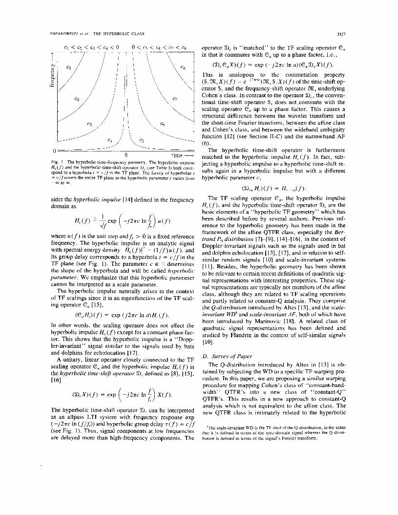
0 time - Fig. 1. The hyperbolic time-frequency geometry. The hyperbolic impulse H,(f) and the hyperbolic time-shift operator D< (see Table I ) both correspond to a hyperbola r = c/fin the TF plane. The family of hyperbolae I = c/fcovers the entire TF plane as the hyperbolic parameter c varies from --OD to 03.

sider the hyperbolic impulse [ 141 defined in the frequency domain as

where U (f) is the unit step andf, > 0 is a fixed reference frequency. The hyperbolic impulse is an analytic signal with spectral energy density I H , (f) 1 = (1 /f ) U ( f ), and its group delay corresponds to a hyperbola t = c/fin the TF plane (see Fig. 1). The parameter c E 2< determines the shape of the hyperbola and will be called hyperbolic parameter. We emphasize that this hyperbolic parameter cannot be interpreted as a scale parameter.

The hyperbolic impulse naturally arises in the context of TF scalings since it is an eigenfunction of the TF scaling operator e, [ 151,

( e , H , > ( f ) = exp ( j 2 n c In a ) H , ( f ) . In other words, the scaling operator does not affect the hyperbolic impulse H , ( f ) except for a constant phase factor. This shows that the hyperbolic impulse is a “Dopp- ler-invariant’’ signal similar to the signals used by bats and dolphins for echolocation [ 171.

A unitary, linear operator closely connected to the TF scaling operator e, and the hyperbolic impulse H , ( f ) is the hyperbolic time-shifr operator Dc defined as [8], [ 151, 1161

The hyperbolic time-shift operator Dc can be interpreted as an allpass LTI system with frequency response exp (-j2nc In (f/fJ) and hyperbolic group delay ~ ( f ) = c / f (see Fig. 1). Thus, signal components at low frequencies are delayed more than high-frequency Components. The

operator 9, is “matched” to the TF scaling operator e, in that it commutes with e, up to a phase factor, i.e.,

(3, eax) (f) = ~ X P ( - j 2 ~ c In a) ( e a DcX) (f). This is analogous to the commutation property (Sr3n,X)(f) = e~’*”‘”(n t ,S ,X) ( f ) ofthe time-shift operator S, and the frequency-shift operator 3n, underlying Cohen’s class. In contrast to the operator Dc, the conventional time-shift operator S, does not commute with the scaling operator ea up to a phase factor. This causes a structural difference between the wavelet transform and the short-time Fourier transform, between the affine class and Cohen’s class, and between the wideband ambiguity function [12] (see Section 11-C) and the narrowband AF (6).

The hyperbolic time-shift operator is furthermore matched to the hyperbolic impulse H,(f). In fact, subjecting a hyperbolic impulse to a hyperbolic time-shift results again in a hyperbolic impulse but with a different hyperbolic parameter c ,

The TF scaling operator e,, the hyperbolic impulse H , ( f ) , and the hyperbolic time-shift operator 33, are the basic elements of a “hyperbolic TF geometry” which has been described before by several authors. Previous reference to the hyperbolic geometry has been made in the framework of the affine QTFR class, especially the Ber- trund Po distribution [7]-[9], [ 141-[ 161, in the context of Doppler-invariant signals such as the signals used in bat and dolphin echolocation [ 131, [ 171, and in relation to self- similar random signals [ IO] and scale-invariant systems [ 1 11. Besides, the hyperbolic geometry has been shown to be relevant to certain recent definitions of quadratic signal representations with interesting properties. These signal representations are typically not members of the affine class, although they are related to TF scaling operations and partly related to constant-Q analysis. They comprise the @distribution introduced by Altes [ 131, and the scale- invariant WD4 and scale-invariant AF, both of which have been introduced by Marinovic [18]. A related class of quadratic signal representations has been defined and studied by Flandrin in the context of self-similar signals [lo].

D. Survey of Paper The Q-distribution introduced by Altes in [13] is ob-

tained by subjecting the WD to a specific TF warping procedure. In this paper, we are proposing a similar warping procedure for mapping Cohen’s class of “constant-bandwidth” QTFR’s into a new class of “constant-Q” QTFR’s. This results in a new approach to constant-Q analysis which is not equivalent to the affine class. The new QTFR class is intimately related to the hyperbolic

4The scale-invariant WD is the TF-dual of the Q-distribution, in the sense that it is defined in terms of the time-domain signal whereas the Q-distribution is defined in terms of the signal’s Fourier transform.

3428 IEEE TRANSACTIONS ON SIGNAL PROCESSING. VOL. 41. NO. 12. DECEMBER 1993

SYMBOL

ST

M” C. De W

W-1

NAME DEFINITION

Time-shift operator Frequency-shift operator ( M Y X ) ( f ) = XU-.)

T F scaling operator

Hyperbolic timeshift operator (vC ~ ) ( f ) = e-jZrcInf; ~ ( f ) Logarithmic frequency warping operator (WX)(f) = X(fr ef l j - )

Exponential frequency warping operator (W-’X)(f) = ,/+ X ( fr lnfr-

( S T X ) ( f ) = e-jz*rf ~ ( f )

( C J ) ( f ) = 4: X ( 6)

TF geometry described above, and is hence called the hyperbolic class (HC). We will show that the HC comprises all QTFR’s that are invariant to TF scalings and hyperbolic time-shifts, and that it is structurally analogous to Cohen’s class. Two prominent QTFR’s, the Bertrand Po distribution and a TF version of the Altes Q-distribution, are members of the HC.

While the HC is not equivalent to the affine QTFR class, it does provide a pertinent framework for constant- Q TF analysis, and is thus related conceptually to the wavelet transform and the affine class. Also, we stress that the HC and the affine class overlap, i .e . , there exist QTFR’s that are invariant to time-shifts, TF scalings, and hyperbolic time-shifts, and thus belong to both classes simultaneously [16], [19]. In particular, the Bertrand Po distribution [8] is a member of both the HC and the affine class.

The paper is organized as follows: In Section 11, we define the HC by applying a “constant-Q warping procedure” to QTFR’s of Cohen class. We derive a description of hyperbolic QTFR’s in terms of two-dimensional kernel functions, and discuss the HC’s relation to the wideband ambiguity function and a “hyperbolic ambiguity function.”

Section I11 shows that the HC can be axiomatically defined as the class of QTFR’s which are invariant to hyperbolic time-shifts and TF scalings. Furthermore, some signal-theoretic fundamentals of the hyperbolic TF geometry on which the HC is based are summarized. In particular, we discuss a hyperbolic signal expansion related to the Mellin transform [8], [13]-[15], [18], [20].

The warping procedure introduced in Section I1 establishes a one-to-one mapping between Cohen’s class and the HC. Any QTFR or any QTFR property of Cohen’s class maps into a corresponding QTFR or QTFR property, respectively, of the HC and vice versa. Section IV discusses corresponding QTFR properties and thereby re- veals further links of the HC to the hyperbolic TF geometry. Some QTFR’s of the HC, which for the most part

correspond to well-known Cohen’s class QTFR’s, are defined and studied in Section V. Finally, Section VI sum- marizes the main results, describes modified versions of the HC, and briefly comments on some further results on the HC which will be included in Part I1 of this paper 1211.

The definitions of some frequently used symbols are summarized in Table I for easy reference.

11. CONSTANT-Q WARPING AND THE HYPERBOLIC CLASS

In [13], Altes proposed a new quadratic signal representation, the Q-distribution, using a mapping that consists of “TF warpings” of the signal and the WD. The Q-distribution has interesting properties (especially “hyperbolic” properties such as a hyperbolic time-shift invariance property and a hyperbolic localization property) and relations with the Mellin transform and the wideband ambiguity function. In this section, we define the HC by applying a similar TF warping mapping to general QTFR’s of Cohen’s class, thereby providing a systematic procedure to convert a “constant-bandwidth” QTFR into a constant-Q QTFR. An alternative axiomatic definition of the new QTFR class will be discussed in Section 111.

A . Constant-Q Warping Given a Cohen’s class QTFR Tic’(t, f ) , we wish to de-

rive a new QTFR Tx( t , f) with constant-Q characteristic, conceptually similar to the wavelet transform or its squared magnitude, the scalogram. To this end, we use a “constant-Q warping” procedure [22] consisting of three steps which are visualized in Fig. 2. In the following, let x ( t ) be analytic, i .e., a signal whose Fourier transform X ( f) is zero forf < 0.

Step 1 : We subject the signal X ( f ) to a logarithmic frequency warping W defined as

2(f) = (WX)(f) L @ X ( f r e f / f . ) , -m < f < 03

(10)

PAPANDREOU Pf a / . : THE. HYPERBOLIC CLASS 3429

fX --

f r fx--.

-

I I

d t

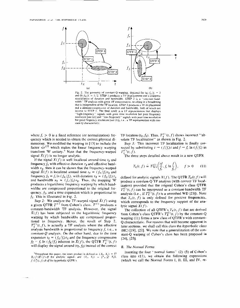
Fig. 2 . The geometry of constant-Q warping, depicted for (a) f x / f r = 2 and (b) f x / f , = 1 /2. STEP 1 produces a TF displacement and a compres- sionidilation of duration and bandwidth. STEP 2 is a “constant-bandwidth” TF analysis with given TF concentration, resulting in a broadening that is independent of the TF location. STEP 3 produces a TF displacement and a dilation/compression of duration and bandwidth, both of which are inverse to STEP 1 . The final result is a TF representation that displays “high-frequency’’ signals with good time resolution but poor frequency resolution [see (a)] and “low-frequency” signals with poor time revolution but good frequency resolution [see (b)], i.e., a TF representation with constant-Q characteristic.

wheref, > 0 is a fixed reference (or normalization) frequency which is needed to obtain the correct physical di- mensions. We modified the warping in [13] to include the factor flr which makes the linear frequency warping transform W ~ n i t a r y . ~ Note that the frequency-warped signal X ( f ) is no longer analytic.

If the signal X ( f ) is well localized around time rx and frequency fx with effective duration T~ and effective bandwidth vX, then it can be shown that the frequency-warped signal X ( f ) is localized around time t g = ( f x / f , ) t x and frequencyfy = f r In (fx/fr), with duration ~g = ( f x / f r ) T~ and bandwidth v y = ( f r / f x ) v x . Thus, the mapping W produces a logarithmic frequency warping by which bandwidths are compressed proportional to the original frequency, fx, and a time expansion which is proportional to fx. This is illustrated in Fig. 2.

Step 2: We analyze the TF-warped signal x ( f ) using a given QTFR T“’ from Cohen’s class. T“’ produces a constant-bandwidth TF analysis. However, the signal x(f) has been subjected to the logarithmic frequency warping by which bandwidths are compressed proportional to frequency. Hence, the result of Step 2, T g ) ( t , f ) , is actually a T F analysis where the effective analysis bandwidth is proportional to frequency f , i.e., a constant-Q analysis. On the other hand, due to the time expansion lx = ( f x / f r ) tx and the frequency compression fg = f r In ( f x / f r ) inherent in X(f), the QTFR T g ’ ( t , f ) will display the signal around ( tx , f x ) instead of the correct

5Throughout this paper, the inner product is defined as ( X , , X , ) = 1; X , ( f ) X : ( f ) df for analytic signals and ( T , . T,) = !?- 10” T,(r, f) 7 ‘ : ( r , f ) dr dffor hyperbolic QTFR’s.

TF location ( t x , f x ) . Thus, TF’(r, f ) shows incorrect “ab- solute TF localization” as shown in Fig. 2.

Step 3: This incorrect TF localization is finally cor- rected by substituting t + ( f / f r ) t and f -+ f , In ( f / f r ) in TF’(r, f ).

The three steps detailed above result in a new QTFR

defined for analytic signals X ( f ) . The QTFR Tx(t,f) will produce a constant-Q TF analysis (with correct T F localization) provided that the original Cohen’s class QTFR Tbc’(t, f ) can be interpreted as a constant-bandwidth T F analysis (i.e., if Tkc’(t, f ) is a smoothed WD 1231). Note that Tx(t, f ) is only defined for positive frequencies, which corresponds to the frequency support of the analytic signal X ( f ) .

The collection of all QTFR’s Tx(t, f ) that are derived from Cohen’s class QTFR’s Tic’ ( t , f ) by the constant-Q warping (1 1) forms a new class of QTFR’s with constant- Q characteristic. For reasons that will become apparent in later sections, we shall call this class the hyperbolic class (HC) [ 191, [22]. We note that a generalization of the constant-Q warping of Cohen’s class has been proposed in 1241, 12-51.

B. The Normal Forms Inserting the four “normal forms” (2)-(5) of Cohen’s

class into (1 l ) , we obtain the following expressions (which we call the Normal Forms I, 11, 111, and IV, re-

3430

spectively) for an arbitrary QTFR T of the HC:

o m o m

* exp [ -j27r (In 5 ) {] dc d{

Vx(b, @)e’2”ffP db do

* Q x ( t ’ , f ’ ) d t ’ d f ’

IEEE TRANSACTIONS ON SIGNAL PROCESSING, VOL 41, NO. 12, DECEMBER 1993

and the ‘‘hyperbolic ambiguity function” [ 181

with the “hyperbolic signal products”

vX(b3 P> ’ 5 uwx( f rb , f r o )

= 5 e h x ( f r eh + B / * ) X* (Leb - ’/2 ), (17)

the TF version of the Q-distribution6 (subsequently called Altes-Marinovic distribution (AD)) [ 131, [ 181

6The original Q-distribution introduced in [13], &(c,f) = j?- X ( f e @ / * ) X * ( f e - @ I 2 ) d p , depends on the (dimensionless) hyperbolic parameter c and the frequency f. The TF version considered here is obtained as Q,(r, f) = fQ,(~,f)l~=,~. A “time-domain” version of the Q-distribution, which is formulated using the time-domain signal x ( r ) instead of the signal’s Fourier transform X(f), was proposed by Marinovic in 1181.

m

= j vx(c, dc

= j Vx(b, /3)eJ2”rb db

--m

m

-m

(19)

One of the advantages of formulating the HC QTFR’s in the specific forms given by (12)-(15), is that the kernels #T(c, SI, W b , P>, +dc, b ) , and *TK, PI are simply scaled versions of the respective kernels of the original Cohen’s class QTFR Tkc’(t, f):

(21)

Hence, these kernels are interrelated by Fourier transforms in exactly the same way as are the respective Cohen’s class kernels (see Fig. 3). Note, however, that the quantities c, {, b, and /3 are dimensionless (i.e., not time or frequency).

According to the normal forms (12)-(15), any member of the HC can be derived from the hyperbolic signal products uX(c , {) and Vx(b, a), the AD Qx(t , f ) , and the hyperbolic AF Bx({, a) by some characteristic unitary, linear 2-D transform. Also, any hyperbolic QTFR is characterized mathematically by any of the four 2-D ker-

Two prominent members of the HC are the AD Qx(r, f ) defined in (18) and the Bertrand Po distribution [6], [8], [9], [14] that is also a member of the affine class. Both distributions will be considered in more detail in Section V.

nels b ( ~ , SI, W b , b>, +Ac, b ) , and *A{, 0).

C. Relation with the Wideband Ambiguity Function The HC can also be expressed in terms of a specific

symmetric version of the wideband ambiguity function ~ 1 , ~ 3 1

xx(r , a) ( S - ~ / ~ ~ ~ - , I ? X , ~ ~ / ~ e ~ 1 / 2 X > = m X ( & f ) X * ( $ = ) df

0

= !i, Vx (In ;, In a) ej2*Tf df 7. (22)

PAPANDREOU et U / . : T H E HYPERBOLIC CLASS 343 I

b\ /C

‘$T(C, b ) Fig. 3 . Fourier transform relations connecting the kemels of the hyperbolic class. (An arrow “ a + b” indicates a Fourier transform from a to b . )

The wideband AF is important in the context of the (wideband) Doppler effect. It can be shown that any member of the HC can be written in terms of the wideband AF as

Correlativr! Correlative Cohen’s class hyperbolic class

m m Cohen’s class Hyperbolic class Tx(t, f) = f 5 5 A7(7f , 0) x,y(7, e’) e’2rrf’ d7 do Fig. 4. Mappings between the energetic Cohen’s class, the correlative

Cohen’s class, the energetic hyperholic class, and the correlative hyperholic class. Note that FT denotes the Fourier transform in the direction of

-m -m

where A T ( { , 0) is a kernel dependent upon T and related to the kernels considered so far, e.g.,

the arrow.

A T ( { , P ) = im aT(- ln 7, P)e-j2”” d r .

For the AD, A a ( { , 6) = so that [13]

D. The Correlative Domain We stress that the wideband AF is not equivalent to the

hyperbolic AF (19) which occurs in the Normal Form IV (15). The hyperbolic AF can be written as the inner product

BXK, P ) = <=,/,e,-, h X , 3I,/,C?,B/ZX) - - (e,-R/23I-{/,x, c , d l 2 9 { / 2 X ) .

Comparing with (22), we see that the main difference is that the wideband AF uses conventional time-shifts S, whereas the hyperbolic AF uses hyperbolic time-shifts The hyperbolic AF is a natural basis for jointly detecting or estimating scale changes and hyperbolic time-shifts in a signal.

The Normal Form IV in (15) can be interpreted in the sense that any hyperbolic QTFR T x ( t , f) is related to a, dual correlative hyperbolic signal representation Tx({, 0) through the following unitary linear transform,

m

. , - J 2 S ( @ C @) dc db.

The dual correlative signal representation fx({, 0) is the hyperbolic AF multiplied by the kernel \k,({, 0) of T [lo],

fx(t, 0) = * T ( { , P)Bx({ , 0). In particular, the corrtlative dual of the AD is the hyperbolic AF itself, i .e., e x ( { , 6) = BX({: 6).

The transform relating T x ( t , f ) and Tx({, 0) establishes a one-to-one correspondence between the “energetic” HC (considered so far) and a dual “correlative” HC whose members are not TF representations but quadratic signal representations depending on the dimensionless quantities { (the hyperbolic-parameter lag) and P (the scale lag). This duality is analogous to the duality of the “energetic” Cohen’s class and a dual “correlative” Cohen’s class [ 11, [4], [23], [26], [27]. In fact, any member Tx({ , P ) of the correlativ? HC can be derived from a corresponding member Tk”(7, v) of the correlative Cohen’s class as

Thus, we have one-to-one correspondences between the energetic Cohen’s class, the correlative Cohen’s class, the

4. d{ dp, energetic HC, and the correlative HC, as depicted in Fig.

3432 IEEE TRAh ISACTIONS ON SIGNAL PROCESSING, VOL. 41, NO. 12, DECEMBER 1993

111. THE HYPERBOLIC PARADIGM In the previous section, the HC has been introduced by

applying a “constant-Q warping” to Cohen’s class. The resulting constant-Q characteristic is however not unique to the HC since it is also featured by many affine QTFR’s. Rather, the specific structure of the HC is its close relation to the hyperbolic TF geometry considered in Section I-C. This relation will be discussed in this and subsequent sections. We first point out an alternative “axiomatic” definition of the HC.

A . Axiomatic Dejinition of the Hyperbolic Class Cohen’s fixed kernel class can be defined by the two

“axioms” (1) of time-shift invariance and frequency-shift invariance, and the HC is derived from Cohen’s class via the constant-Q warping (1 1). We now ask how the axioms of Cohen’s class are transformed under this warping. Ev- idently, the transformed axioms will allow an axiomatic definition of the HC.

Using the inverse of (1 l ) ,

TLc’(t, f ) = Tw-IX(te-f/fr, f , e f l f r ) (23)

where W- ’ , the inverse of the logarithmic-frequency- warping operator W in (lo), is given by

it is easily shown that the time-shift and frequency-shift invariance properties of Cohen’s class transform into the following properties of the corresponding hyperbolic QTFR:

The composite operators W-‘S,W and W-1312vW, which can be considered the images of the time-shift operator S, and the frequency-shift operator 312, under the logarithmic frequency mapping W , can be shown to be the hyperbolic time-shift operator and the T F scaling operator, respectively,

w-’s,w = w-‘m.,w = e&,. Setting c = f r7 and a = e”/&, we finally obtain the result that the HC properties corresponding to the time-shift and frequency-shift invariances of Cohen’s class are the hyperbolic time-shift invariance (previously considered in [16]) and the TF scale invariance, respectively, as stated by the following theorem whose formal proof is outlined in the Appendix.

Theorem: The HC is the class of all QTFR’s which are invariant to hyperbolic time-shifts De and TF scalings e,

according to

This means that the HC can be defined axiomatically by the above two invariance properties with respect to the operators 9, and e,, just as Cohen’s fixed kernel class can be defined by the time-shift and frequency-shift invariance properties, and just as the affine class can be defined by the time-shift and T F scale invariance properties. Note that the scale invariance property Teax(t, f) = Tx(at, f l u ) is an axiom of both the affine class and the HC. In fact, the HC differs from the affine class merely by the fact that the conventional time-shift (S,) is replaced by the hyperbolic time-shift (9J.

B. A Hyperbolic Signal Expansion The fact that the HC is based on the hyperbolic time-

shift operator Dc as discussed in the previous section is a first indication of the HC’s relation to the hyperbolic TF geometry. To obtain a more complete understanding of this relation, we consider a “hyperbolic signal expansion” [8], [14], [15], [18], [28] which constitutes a signal-theoretic foundation of the hyperbolic TF geometry.

Since the family of hyperbolic impulses He ( f ) with --oo < c < 03 covers the entire T F plane according to Fig. 1, it is not surprising that any finite-energy, analytic signal X ( f ) can be written as a superposition of hyperbolic impulses,

X ( f > = jm -CY p x ( c ) H c ( f > d c

P m / r\ J

= 1 px(c) exp ( , - j 2 ~ c In f r -) dc. --03 Jf

The hyperbolic coeflcient function px(c) is the inner product

P X ( C > = ( X , He> = iom x ( f > H , * ( f ) df

The validity of this hyperbolic signal expansion follows easily from the completeness relation

m j Hc(h)H,*( .h) dc = S(h - A ) , h9.h > 0 -m

where 6 ( a ) is the Dirac delta function. In this context, we also note the orthogonality property of hyperbolic impulses

PAPANDREOU r f U / : T H E HYPERBOLIC CLASS 3433

The mapping X(f) + p x ( c ) defined above is essentially the Mellin transform' in the form used in [ 141, [ 151, [20]. It is a unitary, linear transform which is analogous to the inverse Fourier transform X(f) + x ( t ) and which has a number of interesting properties. In particular, we have

PH,(c) = - PD,J(c) = P X ( c -

These relations show that i) the hyperbolic coefficient function of a hyperbolic impulse Hco( f ) is a Dirac impulse at the hyperbolic parameter value c = co; ii) a hyperbolic time-shift (with hyperbolic parameter co) of the signal shifts the hyperbolic coefficient function by co, and iii) a TF scaling of the signal leaves the hyperbolic coefficient function invariant except for an oscillatory phase factor.

The hyperbolic analysis mapping X ( f ) -+ px(c ) is essentially equivalent to the logarithmic frequency warping W used in the previous section for the derivation of the HC. In fact, the inverse Fourier transform of x( f) = (WX) ( f ) defined in (10) is easily shown to be

-f(t) = 4 P X ( f t ) .

This establishes a further strong link of the HC with the hyperbolic paradigm. Note that the hyperbolic signal product ux(c, r) of (16) can now be written as

which yields corresponding expressions also for the AD and the hyperbolic AF,

Further relations between the HC and the hyperbolic TF geometry will be revealed in the next section, which studies corresponding QTFR properties of Cohen's class and the HC.

IV. PROPERTY CORRESPONDENCES The QTFR mapping (1 1) or, equivalently, the kemel

mappings (20), (2 1) establish a one-to-one correspondence between Cohen's class and the new HC, by which any QTFR T'" of Cohen's class is mapped into a QTFR T of the HC. Furthermore, any QTFR property Pee) of Cohen's class maps into a corresponding QTFR property

'In the literature, the Mellin transform is often based on an inner product with weighting function 1 /f, which causes a formal difference from our discussion. If this type of inner product is used, then the hyperbolic impulse H,(f) must be defined without the l/Jffactor.

P in the HC, and vice versa, in the sense that a Cohen's class QTFR satisfies property Pee) if and only if the corresponding hyperbolic QTFR satisfies the corresponding property P.

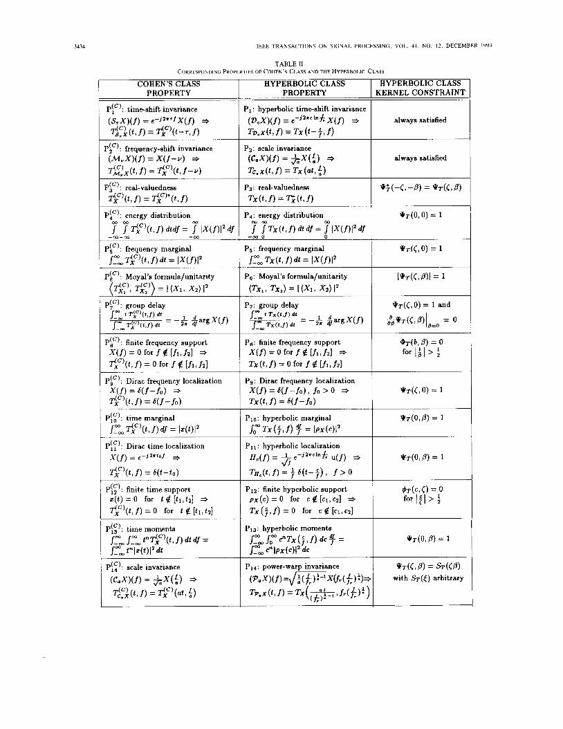
Table I1 lists corresponding QTFR properties and the associated kernel constraints for the HC These kernel constraints are identical to the well-known kernel constraints for Cohen's class [ 11 since, according to (20), (21), the kernels of the two classes are themselves identical up to a scaling by the reference frequency f r .

The study of corresponding QTFR properties provides a means for understanding the structure of the HC, in particular, the HC's relation to the hyperbolic T F geometry. Therefore, some of the correspondences summarized in Table I1 are discussed in the following.

A . Axioms of Cohen 's Class and the Hyperbolic Class It has been shown in Section 111-A that the time-shift

invariance and frequency-shift invariance of Cohen's class (P',') and Pi') in Table 11) map into the hyperbolic time- shift invariance and scale invariance, respectively, in the HC (PI and P2 in Table 11). Thus, the two axioms of Cohen's class map into the axioms of the HC.

B. Identical QTFR Properties in Cdhen's Class and the Hyperbolic Class

The following properties are preserved by the mapping from Cohen's class to the HC: real-valuedness Pi'), energy distribution Pi'), frequency-domain marginal Pi'), unitarity (Moyal's formula) Pi'), group delay Pi'), preservation of frequency support Pi'), and Dirac frequency localization Pb". If a Cohen's class QTFR satisfies any of these properties, then the corresponding hyperbolic QTFR will satisfy this property as well (and vice versa). Note that some of these properties (Pi') and P$"-P$") can be summarized as frequency localization properties.

C. Time Localization Properties Cohen's class properties that are related to time local-

ization (in particular, properties Pi'' and P\;)-P{;) in Ta- ble 11) map into "hyperbolic" properties. A first example is the time-shift invariance property PI') which was shown to map into the hyperbolic time-shift invariance property

i.e., shifting the signal's group delay according to a hyperbolic law produces a hyperbolic time shift in the HC QTFR (cf. Fig. 1). Another important example is the temporal marginal property p!:) of Cohen's class which maps into a "hyperbolic marginal property" [8]

*Note that the signals used in the context of QTFR's or QTFR properties of Cohen's class are not assumed analytic while in the HC they are.

3434

HYPERBOLIC CLASS PROPERTY

IEEE TRANSACTIONS ON SIGNAL PROCESSING, VOL. 41. NO. 12. DECEMBER 1993

HYPERBOLIC CLASS KERNEL CONSTRAINT

TABLE I1 CORRESPONDING PROPERTIES OF COHEN'S CLASS A N D THE HYPERBOLIC CLASS

COHEN'S CLASS PROPERTY

always satisfied

always satisfied

P F ) : real-valuedness TF) ( t , f) = T<Xc"(t, f)

* T ( O , O ) = 1 (c). energy distribution p4m ' m

J J ~ ( 5 c ) : frequency marginal JZ f) dt = lX(f)I2

f) dtdf = 7 IX(f)l' df -m-m - W

P4: energy distribution

s" 7 T x ( t , f ) d t d f = 71X(f)lZdf -m 0

Ps: frequency marginal J-" Tx(t, f) dt = Ix(f)lz P6: Moyal's formula/unitarity (Tx,, Tx, ) = I (Xl I XZ) l2

Pic): Moyal's formula/unitarity (C), TE)) = I (Xl , XZ) IZ

Pa: finite frequency support X ( f ) = 0 for f e [fl, fzl Tx ( t , f) = 0 for f 4 [fl 1 f21

*

Pg : Dirac frequency localization X(f) = w - f o ) 9 fo > 0 T X O , f) = w - f o )

*

Plo: hyperbolic marginal J,"Tx(?,f) 7 = IPX(C)I2

Pi:): Dirac time localization x ( j ) = e - j z r t d * T<Xc'(t, f) = 6 ( t - t o )

PAPANDREOU er a l . : THE HYPERBOLIC CLASS 3435

COHEN’S CLASS PROPERTY

pi:’: axis reversal 5 ( t ) = z ( - t ) , 2( f )=X( - f ) =+- Z y ’ ( t , f) = T<xC’(-t, -f)

PK): weighted convolution x ( f ) = m G ( f ) X ( f ) 3 T p ( t , f )

m

= e-f/fr s GC)(t-t‘, f) T<xC)(t’, f) dt’

Pi:): chirp localization x ( f ) = e- - j rafa j

T<xC’(t, f) = b ( t - a f )

TABLE I1 (Continued.)

HYPERBOLIC CLASS PROPERTY

PIS : timeshift invariance ( s ~ x ) ( ~ ) = e - j z n r f X ( f ) j

Ts,x(t , f) = Tx(t--T, f)

~

Pla: hyperbolic instantan. frequency

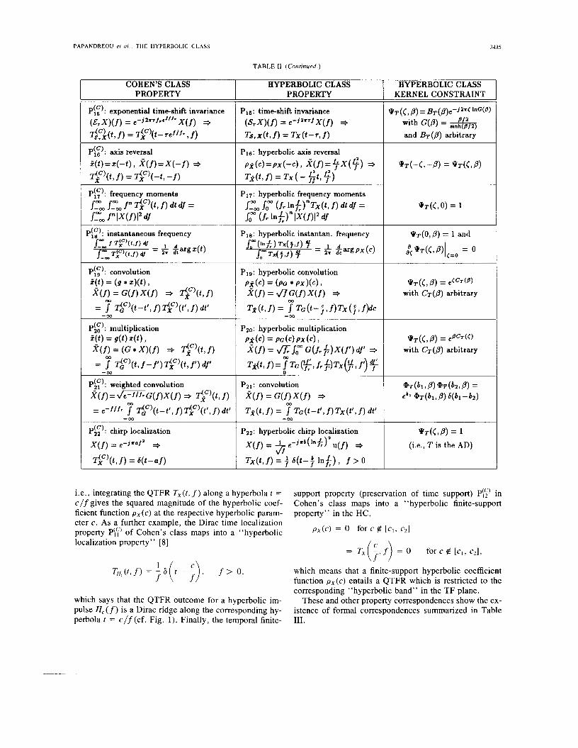
i.e., integrating the QTFR Tx(t, f) along a hyperbola t = c/f gives the squared magnitude of the hyperbolic coefficient function px (c) at the respective hyperbolic parameter c. As a further example, the Dirac time localization property Ply) of Cohen’s class maps into a “hyperbolic localization property” [8]

which says that the QTFR outcome for a hyperbolic impulse H , ( f) is a Dirac ridge along the corresponding hyperbola t = c/f(cf. Fig. 1). Finally, the temporal finite-

HYPERBOLIC CLASS KERNEL CONSTRAINT

q T ( C , P ) = &’(P)e- jZrC InG(’)

with G(P) = & and & ( P ) arbitrary

*T(C, P ) = 1 (i.e., T is the AD)

support property (preservation of time support) in Cohen’s class maps into a “hyperbolic finite-support property” in the HC,

P X ( 4 = 0 for c e [c, 3 c*1

* T x ( ; J ) = 0 fort@ [c , , c21,

which means that a finite-support hyperbolic coefficient function p x ( c ) entails a QTFR which is restricted to the corresponding “hyperbolic band” in the T F plane.

These and other property correspondences show the ex- istence of formal correspondences summarized in Table 111.

3436

COHEN’S CLASS

straight line in the TF plane t = t o

JEEE TRANSACTIONS ON SIGNAL PROCESSING, VOL. 41. NO. 12, DECEMBER 1993

HYPERBOLIC CLASS

hyperbola in the TF plane

t = c/f time-domain signal

z ( t ) instantaneous power

hyperbolic coefficient function

PX (4 “hyperbolic power”

D. Scale Invariance where

maps into the “power-warp invariance” property The scale invariance property Pi:) in Cohen’s class ( E , x ) ( ~ ) A exp ( - j 2 ~ r f ~ e f ’ f r ) x ( f ) .

Note that the “exponential time-shift operator” E, is an allpass LTI system with exponential group delay T ( f ) = ,t?f/fr.

v. SOME MEMBERS OF THE HYPERBOLIC CLASS Due to the one-to-one mapping between Cohen’s class

and the HC, any QTFR T“’ of Cohen’s class is mapped into a QTFR T of the HC. As a result, well-known

where

Cohen’s class QTFR’s such as the (generalized) WD, the ( @ , X ) ( f ) d r X(h (:)I”) , a > 0 spectrogram, the smoothed pseudo-WD, the (generalized)

Choi-Williams distribution, the Butterworth distribution

T , , x ( t , f ) = Tx

in the HC. The linear operator 6, produces a fre uency warping according to a power law f + fr(f / fr)17‘; the factor J<1 / a ) (f / f i)”/‘’p assures the unitarity of the power-warp operator 6,. The subclass of “power-warp invariant” hyperbolic QTFR’s is the counterpart of the shift-scale invariant subclass of Cohen’s class [ 4 ] , [29 ] . We note that the power-warp operator 6, can be used to map the affine class to new classes of QTFR’s that satisfy scale invariance and generalized time shift invariance 1301.

E. Exponential Time-Shift Invariance While the conventional time-shift invariance is not a

“natural” property inside the HC, there do exist hyperbolic QTFR’s that satisfy the time-shift invariance property (e.g., the Bertrand Po distribution [ S I ) . These QTFR’s are simultaneously members of the HC and the affine QTFR class; in fact, they form the intersection of the two classes [16 ] , [ 1 9 ] , [ 2 1 ] .

The Cohen’s class property corresponding to the time- shift invariance property in the HC is the “exponential time-shift invariance property” P$:)

~ k t k ( t , f ) = ~ k ” ( t - Teflfr, f )

etc. [ l ] , can be converted into hyperbolic QTFR’s satisfying the hyperbolic time-shift invariance and the scale invariance as well as other desirable properties. Con- versely, using the inverse mapping ( 2 3 ) , we can also con- struct Cohen’s class QTFR’s corresponding to interesting hyperbolic QTFR’s [ 191, [22] such as the Bertrand Po distribution.

This section considers some specific QTFR’s of the HC. We start with a discussion of the two most prominent hyperbolic QTFR’s, the Altes-Marinovic distribution and the Bertrand Po distribution. All hyperbolic QTFR’s discussed are listed in Table IV together with the corresponding QTFR’s of Cohen’s class. Table V shows the QTFR kernels and the QTFR properties satisfied.

A. The Altes-Marinovic Distribution The Altes-Marinovic distribution (AD) [ 131, [ 181, [22]

PAPANDREOU er 01 : THE HYPERBOLIC CLASS 3431

TABLE IV CORRESPONDING QTFR’S OF COHEN’S CLASS AND THE HYPERBOLIC CLASS

(NOTETHATU,(~ . 7) = x ( t + 7 / 2 ) x * ( r ~ 7/2), U , ( f , U) = x ( f + U/2)X*(f- V / 2 ) , ANDZi,(C, r) AND V, (h , 0) AREGIVEN BY (16),

(17). A N D (2.5). RESPECTIVELY)

COHEN’S CLASS QTFR T(xC)(t, f) Wigner distribution

Wx(t, f) = J ux(t, r ) e - j z * f r d r m

-m m

= J Ux(f, u ) e j Z r t u du

= J X ( f + ;) X* (f- 5) ejzI tu du

-m m

--m

Generalized Wigner distribution

Wg’(t, f) = J ux( t+ar , r ) e - J z * f r d r m

-m m

-m = Ux( f -au, U) e jzXtu du

Cohen-Bertrand distribution

Pic’(t,f) = J Ux(f+fr l n G ( t ) , u ) e j Z r t u d u

with G(p) = & Spectrogram

sX(t, j) = I J ~ ( f ’ ) ~ * ( f ’ - j ) ejz*tf’ df’ 1’ = J J Wi.(t’-t,f’-f)Wx(t’,f’)dt‘df’

m

-m

m

-m m m

-m -m

with F(f) = r ( f r e f / f r . ) Pseudo Wigner distribution

PWDx(t , f ) =

= 7 uf(0, T ) ux(t , r ) e - j z r f r d r -m

= s” WdO, f-f’) Wx(t, f’) df’ -m

with F(f) = m r(fr e f / f r ) Smoothed Pseudo Wigner distribution SPWDx(t, f) =

= 7 i(t--2‘) PWDx ( t ’ , f) dt’

= J J i(t-t‘) q(O, r ) ux(t’, r ) e- j2*frdt’dr -m m o o

-m-m m m

= J J i(t-4’) WF(0, f-1’) Wx(t’, f’) dt’df‘ -m-m

with i ( t ) = frs(frt), i’(f) = m I ‘ ( f r e f / f r )

HYPERBOLIC CLASS QTFR Tx(t, f) Altes-Marinovic distribution

Qx( t , f ) = J ux(tf,C) e - ’ z * ( l n k ) c d(‘ m

-m m

= J Vx (lnf;, p) e jzr t fP dp -m

Bertrand distribution

J‘x(t, f) = J Vx (ln(f;G(P)), 0) e jz* l fP dp

with G(p) = & Hyperbologram

Yx(t,f) = $ 1 TX(f’)I’*($f‘) gzrtf1”$ df’

m

-m

0 IZ m o o

= J JQr(kfi(t’f‘-tf), fr$)Q~(t’,f’)dt’df’ -m 0

Pseudo Altes-Marinovic distribution

PADx 0, f) = m

= f r J U r ( 0 , C ) ux(tf,C) e - j z * ( l n k ) c dC

= f r J Qr (0, f r fi, QX ( 3 9 f’) $ -m m

Smoothed Pseudo Altes-Marinovic distribution SPADx(t, f) =

= 7 s ( t f - c ) PADx (f , f) d c -m

m m

= fr J J .(if*) ur(0, C ) ux(c, C ) e-’z*(lnf;)cdcd(

= fr -m J J 0 4 t f - c ) Qr (0, f r f i ) QX ( +, f’) dc$

-m-m m m

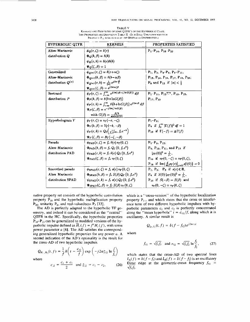
is the hyperbolic counterpart of the WD [l], [23], [31] in Cohen’s class. The AD’S kernels are particularly simple,

the AD is not a member of the affine QTFR class. The AD is the only member of the HC that satisfies the hyperbolic chirp localization property P22. Several sets of other QTFR properties can alternatively be used to uniquely define the AD inside the HC, in the sense that the AD is the only member of the HC that satisfies these properties. One such property set consists of the marginal properties P, and Plo, the finite-support properties PS and P,*, unitarity P6, and real-valuedness P3 [32]. An alter-

$Q(Cj s-1 = 6(c), @Q(b, p) = 6(b),

b, = 6 ( c ) 6(b), *e({ , 0) = 1.

According to Table V , the AD satisfies all QTFR properties listed in Table I1 except for the conventional time- shift invariance property P15. Since PI, is not satisfied,

3438 IEEE TRANSACTIONS ON SIGNAL PROCESSING, VOL. 41. NO. 12, DECEMBER 1993

TABLE V KERNELS AND PROPERTIES OF SOME Q T F R ’ S OF THE HYPERBOLIC CLASS.

THE PROPERTIES ARE DEFINED IN TABLE 11. (IT IS STILL UNKNOWN WHETHER PROPERTY P,, IS SATISFIED BY THE BERTRAND DISTRIBUTION)

Generalized Altea-Marinovic distribution Q(”)

Bertrand distribution P

Hyperbologram Y

Pseudo Altes-Marinovic distribution PAD

Smoothed pseudo Altes-Marinovic distribution SPAD

native property set consists of the hyperbolic convolution property PI9 and the hyperbolic multiplication property P20, unitarity P,, and real-valuedness P3 [33].

The AD is perfectly adapted to the hyperbolic TF geometry, and indeed it can be considered as the “central” QTFR in the HC. Specifically, the hyperbolic properties PIO-Pl3 can be generalized to modified versions of the hyperbolic impulse defined as E,. ( f ) = f” H,. ( f ), with some power parameter a [8]. The AD satisfies the corresponding generalized hyperbolic properties for any power a. A second indication of the AD’S optimality is the result for the cross-AD of two hyperbolic impulses

where

which is a ‘ ‘cross-version’’ of the hyperbolic localization property PI1 , and which states that the cross or interference term of two different hyperbolic impulses with hyperbolic parameters c1 and c2 is perfectly concentrated along the “mean hyperbola” t = cI2/f, along which it is oscillatory. A similar result is

where

which states that the cross-AD of two spectral lines Lfl( f ) = 6 (f - fi) and Lf2( f ) = 6 ( f - f2) is an oscillatory Dirac ridge at the geometric-mean frequency f i 2 =

%.

PAPANDREOU rr U / . : THE HYPERBOLIC CLASS 3439

Since the WD is known to feature perfect concentration in the case of linear FM signals (chirp signals) X(f) = e-JTap, an analogous result must hold for the AD. The frequency-warped version (W-’X) ( f ) of the linear-FM chirp signal can be shown to be (up to a constant factor) the “hyperbolic chirp signal” Pb(f) = ( l / J f ) exp [ - j ~ b ( I n ( f / f r ) ) 2 ] u ( f ) (where b = af: is a “hyperbolic chirp rate” and U ( f ) is the unit step), whose group delay is ~ ( f ) = ( b / f ) In ( f / f , ) . The AD of the hyperbolic chirp signal defined above is indeed a Dirac ridge along the group delay curve t = T ( f),

Bertrand distribution (BD) in the f o l l ~ w i n g , ~

= S , X ( f F ( S ) + i ) X * ( f F ( i ) - ;)

= f im X(fG(p)e’ / l”)X*(fG(/3)e-01/2) - m

This property suffices to uniquely define the AD inside the HC.

. G(P) eJ2Tr fp do

where“

B. The Generalized Altes-Marinovic Distribution P P t e-’/’ F(P) = 2 coth - = 2 ,Dl2 - , - p p 9

Many of the properties of the AD can be extended to 2 the family of hyperbolic QTFR’s depending on a real-valued parameter a [22]

n m

which we call generalized Altes-Murinovic distribution (GAD). The GAD is the hyperbolic counterpart of the generalized Wigner distribution [4], [23], [29], [32] of Cohen’s class. Note that the AD is reobtained as a special case for a = 0, and is the only GAD which is real-valued. The interference term concentration properties of the AD, (26) and (27), can be extended to the GAD, but with an a-dependent displacement of the interference term loca- tions.

Two of the kemels of the BD are simple functions,

QP(b, 0) = 6(b + In G(P)), qp({ , 0) = e-J2TcinC‘P).

The BD satisfies many of the desirable properties listed in Table 11. The main feature of the BD (from a HC viewpoint) is that the BD satisfies the conventional time-shift invariance property P is . Thus, it is also a member of the affine QTFR class; indeed, i t may be considered as the central QTFR inside the HC subclass that forms the intersection between the HC and the affine class [ 191, [2 I ] . Inside the HC, the BD is uniquely defined by the time- shift invariance property PI5 and the hyperbolic marginal property P lo (or, equivalently. the hyperbolic localization

From the viewpoint of the a 8 n e QTFR class, the BD is unique because of the hyperbolic properties it satisfies. Indeed, inside the affine class, the BD is uniquely defined by the hyperbolic time-shift invariance property PI and the hyperbolic marginal property P (or, equivalently, the hyperbolic localization property P i I). Other property sets defining the BD are discussed in [6], [8].

Since the BD is a prominent member of the HC, it is interesting to see to which member of Cohen’s class the BD corresponds. Using the relation (23), the Cohen’s class counterpart of the BD (abbreviated CBD in the fol-

property PI

‘It is interesting that the “affine Wigner distribution” proposed by Shenoy and Parks in [20] is essentially the BD. (In this context. we note that a factor p ( x ) is missing inside the integral in 120, eq. (16)].

X , , ( ~ ) P - ~ ’ ~ -. where A,,@) and p , , ( p ) are the functions used in [ X I .

C. The Bertrand Distribution Another prominent member of the HC is the Bertrand

l o N o t e !hat F ( p ) = ( I / 2 ) ( + -p)) and G ( p ) = p,l(p) == Po distribution [6], [8], (91, [ 141, [20], [22], briefly called

3440 IEEE TRANSACTIONS ON SIGNAL PROCESSING, VOL. 41, NO. 12. DECEMBER 1993

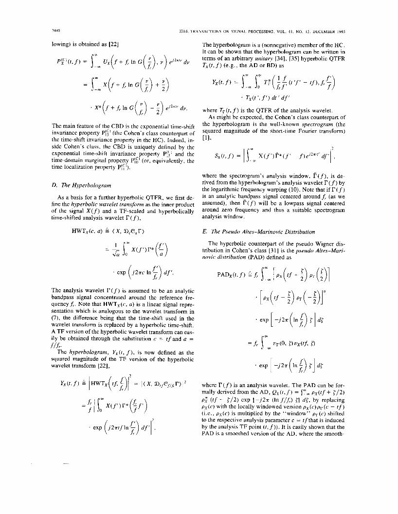
lowing) is obtained as [22] The hyperbologram is a (nonnegative) member of the HC. It can be shown that the hyperbologram can be written in terms of an arbitrary unitary [34], [35] hyperbolic QTFR T x ( t , f ) (e.g., the AD or BD) as

m

P‘c’(t’ f, = i-, ux(f -k f r In ‘( i) ’ ’) dv

- X * ( f + f l n G (i) - i) eJ2*‘” dv.

The main feature of the CBD is the exponential time-shift invariance property P\s’ (the Cohen’s class counterpart of the time-shift invariance property in the HC). Indeed, inside Cohen’s class, the CBD is uniquely defined by the exponential time-shift invariance property Pis) and the time-domain marginal property Pi:’ (or, equivalently, the time localization property pry)).

Tx(t ’, f’) dt ’ d f ’

where Tr ( t , f ) is the QTFR of the analysis wavelet. As might be expected, the Cohen’s class counterpart of

the hyperbologram is the well-known spectrogram (the squared magnitude of the short-time Fourier transform) [117

S x ( t , f ) = 1 iW X ( f ’ ) F * ( f ‘ - f)e’2”‘f’ - m

where the spectrogram’s analysis window, f ( f ) , is derived from the hyperbologram’s analysis wavelet r ( f ) by the logarithmic frequency warping (10). Note that if r ( f ) is an analytic bandpass signal centered around f r (as we assumed), then f (f) Will be a lowpass signal centered

zero frequency and thus a suitable Spectrogram analysis window.

D. The Hyperbologram

As a basis for a further hyperbolic QTFR, we first define the hyperbolic wavelet transform as the inner product of the signal X(f) and a TF-scaled and hyperbolically time-shifted analysis wavelet r (f),

HWT,(c, a ) (X, a>,C?,r) E. The ‘Pseudo Altes-Marinovic Distribution

m

& o

The hyperbolic counterpart of the pseudo Wigner distribution in Cohen’s class [3 11 is the pseudo Altes-Mari- novic distribution (PAD) defined as

= .L j x ( f i ) r * c )

* exp ( j 2 n c ln;) df ’.

The analysis wavelet r ( f ) is assumed to be an analytic bandpass signal concentrated around the reference frequencyf,. Note that HWTx(c, a ) is a linear signal representation which is analogous to the wavelet transform in (7), the difference being that the time-shift used in the wavelet transform is replaced by a hyperbolic time-shift. A TF version of the hyperbolic wavelet transform can easily be obtained through the substitution c = t f and a =

The hyperbologram, Yx(t , f ) , is now defined as the squared magnitude of the TF version of the hyperbolic wavelet transform [22],

f/h.

* exp [ -j2n(ln;) {] d{

r m

exp [ - j 2 n ( l n i ) {] d r

y x ( t , f ) HWT, t f , - = i ( ~ , a>,,ef/hr)12 where r ( f ) is an analysis wavelet. The PAD can be formally derived from the AD, Q , ( t , f ) = jZW px(tf + {/2) P,* ( t f - {/2) exp [- j2n (In f / f r ) {I d { , by replacing px(c) with the locally windowed version p x ( C ) p r ( c - tf) (i.e., px(c) is multiplied by the “window” p r ( c ) shifted to the respective analysis parameter c = tfthat is induced by the analysis TF point ( l , f ) ) . It is easily shown that the PAD is a smoothed version of the AD, where the smooth-

I ( :ii? = 4 1 Som x(f’)r* @ - I ) f

. exp ( j2~tf ln;) df’12.

PAPANDREOU er al . : THE HYPERBOLIC CLASS 344 1

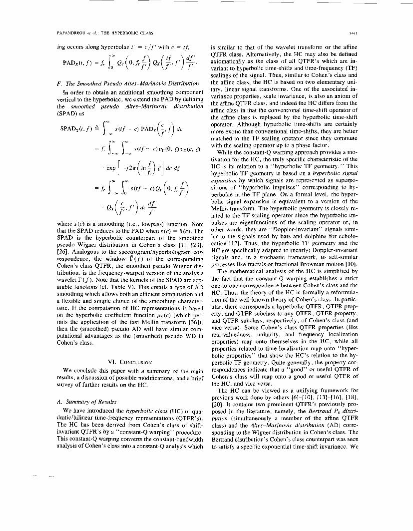
ing occurs along hyperbolae t‘ = c / f ’ with c = t f ,

F. The Smoothed Pseudo Altes-Marinovic Distribution In order to obtain an additional smoothing component

vertical to the hyperbolae, we extend the PAD by defining the smoothed pseudo Altes-Marinovic distribution (SPAD) as

,m I ,

SPAD,(t, f ) 51, s(tf - C ) PADx(; dc f)

* exp [ - j27r ( ln i ) i.] d c d l

where s(c) is a smoothing (i.e., lowpass) function. Note that the SPAD reduces to the PAD when s ( c ) = 6 ( c ) . The SPAD is the hyperbolic counterpart of the smoothed pseudo Wigner distribution in Cohen’s class [ l ] , [23], [26]. Analogous to the spectrogram/hyperbologram correspondence, the window f ( f ) of the corresponding Cohen’s class QTFR, the smoothed pseudo Wigner distribution, is the frequency-warped version of the analysis wavelet r (f). Note that the kernels of the SPAD are sep- arable functions (cf. Table V). This entails a type of AD smoothing which allows both an efficient computation and a flexible and simple choice of the smoothing characteristic. If the computation of HC representations is based on the hyperbolic coefficient function p x (c) (which per- mits the application of the fast Mellin transform [36]), then the (smoothed) pseudo AD will have similar com- putational advantages as the (smoothed) pseudo WD in Cohen’s class.

VI. CONCLUSION We conclude this paper with a summary of the main

results, a discussion of possible modifications, and a brief survey of further results on the HC.

A, Summary of Results We have introduced the hyperbolic class (HC) of qua-

dratidbilinear time-frequency representations (QTFR’s). The HC has been derived from Cohen’s class of shift- invariant QTFR’s by a “constant-Q warping’’ procedure. This constant-Q warping converts the constant-bandwidth analysis of Cohen’s class into a constant-Q analysis which

is similar to that of the wavelet transform or the affine QTFR class. Alternatively, the HC may also be defined axiomatically as the class of all QTFR’s which are invariant to hyperbolic time-shifts and time-frequency (TF) scalings of the signal. Thus, similar to Cohen’s class and the affine class, the HC is based on two elementary unitary, linear signal transforms. One of the associated invariance properties, scale invariance, is also an axiom of the affine QTFR class, and indeed the HC differs from the affine class in that the conventional time-shift operator of the affine class is replaced by the hyperbolic time-shift operator. Although hyperbolic time-shifts are certainly more exotic than conventional time-shifts, they are better matched to the TF scaling operator since they commute with the scaling operator up to a phase factor.

While the constant-Q warping approach provides a mo- tivation for the HC, the truly specific characteristic of the HC is its relation to a “hyperbolic TF geometry.” This hyperbolic TF geometry is based on a hyperbolic signal expansion by which signals are represvted as superpo- sitions of ‘‘hyperbolic impulses” corresponding to hyperbolae in the TF plane. On a formal level, the hyperbolic signal expansion is equivalent to a version of the Mellin transform. The hyperbolic geometry is closely related to the TF scaling operator since the hyperbolic impulses are eigenfunctions of the scaling operator or, in other words, they are “Doppler-invariant” signals similar to the signals used by bats and dolphins for echolocation [17]. Thus, the hyperbolic TF geometry and the HC are specifically adapted to (nearly) Doppler-invariant signals and, in a stochastic framework, to self-similar processes like fractals or fractional Brownian motion [ 101.

The mathematical analysis of the HC is simplified by the fact that the constant-Q warping establishes a strict one-to-one correspondence between Cohen’s class and the HC. Thus, the theory of the HC is formally a reformula- tion of the well-known theory of Cohen’s class. In particular, there corresponds a hyperbolic QTFR, QTFR property, and QTFR subclass to any QTFR, QTFR property, and QTFR subclass, respectively, of Cohen’s class (and vice versa). Some Cohen’s class QTFR properties (like real-valuedness, unitarity , and frequency localization properties) map onto themselves in the HC, while all properties related to time localization map onto “hyperbolic properties” that show the HC’s relation to the hyperbolic T F geometry. Quite generally, the property correspondences indicate that a “good” or useful QTFR of Cohen’s class will map onto a good or useful QTFR of the HC, and vice versa.

The HC can be viewed as a unifying framework for previous work done by others [6]-[IO], [13]-[161, 1181, [20]. It contains two prominent QTFR’s previously proposed in the literature, namely, the Bertrand Po distribution (simultaneously a member of the affine QTFR class) and the Altes-Marinovic distribution (AD) corresponding to the Wigner distribution in Cohen’s class. The Bertrand distribution’s Cohen’s class counterpart was seen to satisfy a specific exponential time-shift invariance. We

3442 IEEE TRANSACTIONS ON SIGNAL PROCESSING. VOL. 41. NO. 12, DECEMBER 1993

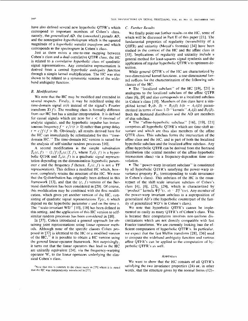
have also defined several new hyperbolic QTFR’s which correspond to important members of Cohen’s class, namely, the generalized AD, the (smoothed) pseudo AD, and the nonnegative hyperbologram which is the squared magnitude of a hyperbolic wavelet transform and which corresponds to the spectrogram in Cohen’s class.

Just as there exists a one-to-one mapping between Cohen’s class and a dual correlative QTFR class, the HC is related to a correlative hyperbolic class of quadratic signal representations. Any correlative representation is derived from a central hyperbolic ambiguity function through a simple kemel multiplication. The HC was also shown to be related to a symmetric version of the wideband ambiguity function.

B. Modijications We note that the HC may be modified and extended in

several respects. Firstly, it may be redefined using the time-domain signal x ( t ) instead of the signal’s Fourier transform X(f). The resulting class is formally different from our HC but has a similar interpretation. It is defined for causal signals which are zero for r < 0 (instead of analytic signals), and the hyperbolic impulse has instantaneous frequencyf = c / t ( t > 0) rather than group delay r = c/f(f > 0). Obviously, all results derived here for the HC can immediately be reformulated for this “time- domain HC.” The time-domain HC version is suited for the analysis of self-similar random processes [ 101.

A second modification is the simple substitution

bolic QTFR and T x ( c , f ) is a quadratic signal representation depending on the dimensionless hyperbolic parameter c and the frequency f (hence, Fx(c, f ) is not a TF representation). This defines a modified HC which, however, completely retains the structure of the HC. We note that the Q;distribution has originally been defined in this framework [13], and that the ( c , f)-version of the Ber- trand distribution has been considered in [20]. Of course, this modification may be combined with the first modification, which gives yet another version of the HC, consisting of quadratic signal representations Ti (c , r ) which depend on the hyperbolic parameter c and on the time t . The “scale-invariant WD” [ 101, [ 181 has been defined in this setting, and the application of this HC version to self- similar random processes has been considered in [ lo].

In [37], Cohen introduced a general approach for obtaining joint representations using linear operator methods. Although none of the specific classes Cohen proposed in [37] is identical to the HC or a modified version of the HC,” it is possible to obtain a HC version using the general linear-operator framework. Not surprisingly, it turns out that the linear operators that lead to the HC are unitarily equivalent [24], via the frequency-warping operator W, to the linear operators underlying the clas- sical Cohen’s class.

Fx,<c,f> = (l/f)_T,(c/f, f), where Tx(t, f) is a hyper-

“Note that this is contrary to the claim made in [25] where it is stated that the HC was independently introduced in [37]

C. Further Results We finally point out further results on the HC, some of

which will be discussed in Part I1 of this paper [21]. The fundamental properties of regularity (reversibility of a QTFR) and unitarity (Moyal’s formula) [34] have been studied in the context of the HC and the affine class in [35]. Implications of regularity and unitarity include a general method for least-squares signal synthesis and the application of regular hyperbolic QTFR’s to optimum de- tection.

While general QTFR’s of the HC are characterized by two-dimensional kernel functions, a one-dimensional kernel suffices for the characterization of the following sub- classes of the HC.

The “localized subclass” of the HC [19], [21] is analogous to the localized subclass of the affine QTFR class [6], [9] and also corresponds to a localized subclass in Cohen’s class [ 191. Members of this class have a simplified kemel aT(b, 0) = B,(P) 6(b - A T ( @ ) ) param- eterized in terms of two 1-D “kemels” A T @ ) and B T ( P ) . Both the Bertrand distribution and the AD are members of this subclass.

The “affine-hyperbolic subclass” [16], [19], [21] comprises all hyperbolic QTFR’s which are time-shift invariant and which are thus also members of the affine QTFR class. This subclass forms the intersection of the affine class and the HC, and is part of both the localized hyperbolic subclass and the localized affine subclass. Any affine-hyperbolic QTFR can be derived from the Bertrand distribution (the central member of the affine-hyperbolic intersection class) via a frequency-dependent time convolution.

The “power-warp invariant subclass” is constituted by all hyperbolic QTFR’s satisfying the power-warp invariance property PI4 (corresponding to scale invariance in Cohen’s class). This subclass of the HC is the counterpart of the shift-scale invariant subclass of Cohen’s class [4], [6], [23], [29], which is characterized by “product” kemels \kkC’(7, v) = S$”(TV). Any member of the power-warp invariant subclass is a superposition of generalized AD’S (the hyperbolic counterpart of the family of generalized WD’s in Cohen’s class).

We note that hyperbolic QTFR’s cannot be imple- mented as easily as many QTFR’s of Cohen’s class. This is because their computation involves non-uniform dis- cretizations which are not directly compatible with fast Fourier transforms. We are currently looking into the efficient computation of hyperbolic QTFR’s. In particular, we expect that the fast Mellin transform [28], [36] used to compute the wideband ambiguity function and various affine QTFR’s can be applied to the computation of hyperbolic QTFR’s as well.

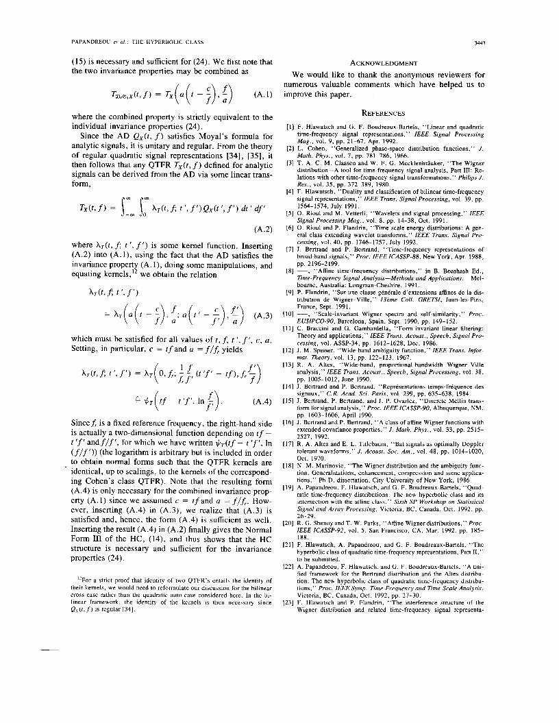
APPENDIX We want to show that the HC consists of all QTFR’s

satisfying the two invariance properties (24) or, in other words, that the structure given by the normal forms (12)-

PAPANDREOU et U / . : THE HYPERBOLIC CLASS 3443

(15) is necessary and sufficient for (24). We fiist note that the two invariance properties may be combined as

where the combined property is strictly equivalent to the individual invariance properties (24).

Since the AD Qx(t , f ) satisfies Moyal’s formula for analytic signals, it is unitary and regular. From the theory of regular quadratic signal representations [34], [35], it then follows that any QTFR T,(t, f ) defined for analytic signals can be derived from the AD via some linear transform,

Tx(t,f) = im im M,f; t’,f’)Qx<r’,f’> a’r’df’ - m 0

(A. 2)

where A&, f; r ’, f ’ ) is some kernel function. Inserting (A.2) into (A.l ) , using the fact that the AD satisfies the invariance property (A. l ) , doing some manipulations, and equating kernels,I2 we obtain the relation

AT(t, f; ’> f‘)

= AT(a(r - i ) , : ; a ( r ’ - ; ) , c ) (A.3)

which must be satisfied for all values of t , f, t ’, f’, c, a . Setting, in particular, c = rfand a = f/fr yields

Sincef, is a fixed reference frequency, the right-hand side is actually a two-dimensional function depending on t f - t ’f’ andflf’, for which we have written 1c/T(tf - t ’f’, In (flf’)) (the logarithm is arbitrary but is included in order to obtain normal forms such that the QTFR kernels are identical, up to scalings, to the kernels of the corresponding Cohen’s class QTFR). Note that the resulting form (A.4) is only necessary for the combined invariance property (A. 1) since we assumed c = t f and a = f/fr. How- ever, inserting (A.4) in (A.3), we realize that (A.3) is satisfied and, hence, the form (A.4) is sufficient as well. Inserting the result (A.4) in (A.2) finally gives the Normal Form I11 of the HC, (14), and thus shows that the HC structure is necessary and sufficient for the invariance properties (24).

”For a strict proof that identity of two QTFR’s entails the identity of their kernels, we would need to reformulate our discussion for the bilinear cross case rather than the quadratic auto case considered here. In the bilinear framework, the identity of the kernels is then necessary since Q , ( f , f ) is regular 1341.

ACKNOWLEDGMENT We would like to thank the anonymous reviewers for

numerous valuable comments which have helped us to improve this paper.

REFERENCES [ l ] F. Hlawatsch and G. F. Boudreaux-Bartels, “Linear and quadratic

time-frequency signal representations,” IEEE Signal Processing Mag. , vol. 9 , pp. 21-67, Apr. 1992.

[2] L. Cohen, “Generalized Dhase-soace distribution functions.” J . Math. Phys . , vol. 7 , pp. 781-786,’1966. T. A. C. M. Claasen and W. F. G. Mecklenbrauker, “The Wigner distribution-A tool for time-frequency signal analysis, Part 111: Re- lations with other time-frequency signal transformations,” Philips J. Res., vol. 35, pp. 372-389, 1980. F. Hlawatsch, “Duality and classification of bilinear time-frequency signal representations,” IEEE Trans. Signal Processing, vol. 39, pp.

0. Rioul and M. Vetterli, “Wavelets and signal processing,” IEEE Signal Processing M a g . , vol. 8 , pp. 14-38, Oct. 1991. 0. Rioul and P. Flandrin, “Time-scale energy distributions: A general class extending wavelet transforms,” IEEE Trans. Signal Pro- cessing, vol. 40, pp. 1746-1757, July 1992. J . Bertrand and P. Bertrand, “Time-frequency representations of broad-band signals,” Proc. IEEE ICASSP-88, New York, Apr. 1988,

-, “Affine time-frequency distributions,” in B. Boashash Ed., Time-Frequency Signal Analysis-Methods and Applications. Mel- bourne, Australia: Longman-Cheshire, 1991. P. Flandrin, “Sur une classe genirale d’extensions affines de la distribution de Wigner-Ville,” 13Pme Coll. GRETSI, Juan-les-Pins, France, Sept. 1991. - , “Scale-invariant Wigner spectra and self-similarity,” Proc. EUSIPCO-90, Barcelona, Spain, Sept. 1990, pp. 149-152. C. Braccini and G. Gambardella, “Form-invariant linear filtering: Theory and applications,” IEEE Trans. Acoust. , Speech, Signal Pro- cessing, vol. ASSP-34, pp. 1612-1628, Dec. 1986. J . M. Speiser, “Wide-band ambiguity function,” IEEE Trans. Infor- mar. Theory, vol. 13, pp. 122-123, 1967. R. A. Altes, “Wide-band, proportional-bandwidth Wigner-Ville analysis,” IEEE Trans. Acoust. , Speech, Signal Processing, vol. 38, pp. 1005-1012, June 1990. J. Bertrand and P. Bertrand, “Reprhentations temps-frCquence des signaux,” C.R. Acad. Sci. Paris, vol. 299, pp. 635-638, 1984. J. Bertrand, P. Bertrand, and J. P. Ovarlez, “Discrete Mellin transform for signal analysis,” Proc. IEEE ICASSP-90, Albuquerque, NM, pp. 1603-1606, April 1990. J. Bertrand and P. Bertrand, “A class of affine Wigner functions with extended covariance properties,” J . Math. Phys . , vol. 33, pp. 2515- 2527, 1992. R . A. Altes and E. L. Titlebaum, “Bat signals as optimally Doppler tolerant waveforms,” J. Acoust. Soc. A m . , vol. 48, pp. 1014-1020, Oct. 1970. N. M. Marinovic, “The Wigner distribution and the ambiguity function: Generalizations, enhancement, compression and some applications,” Ph.D. dissertation, City University of New York, 1986. A. Papandreou, F. Hlawatsch, and G. F. Boudreaux-Bartels, “Quad- ratic time-frequency distributions: The new hyperbolic class and its intersection with the affine class,” Sixth SP Workshop on Staristical Signal and Array Processing, Victoria, BC, Canada, Oct. 1992, pp.

R. G. Shenoy and T. W. Parks, “Affine Wigner distributions,” Proc. IEEE ICASSP-92, vol. 5 , San Francisco, CA, Mar. 1992, pp. 185- 188. F. Hlawatsch, A. Papandreou, and G. F. Boudreaux-Bartels, “The hyperbolic class of quadratic time-frequency representations, Part 11,” to be submitted. A. Papandreou, F. Hlawatsch. and G. F. Boudreaux-Bartels, “A uni- fied framework for the Bertrand distribution and the Altes distribution: The new hyperbolic class of quadratic time-frequency distributions,” Proc. IEEE Symp. Time-Frequency and Time-Scale Analysis, Victoria, BC, Canada, Oct. 1992, pp. 27-30. F. Hlawatsch and P. Flandrin, “The interference structure of the Wigner distribution and related time-frequency signal representa-

1564-1574, July 1991.

pp. 2196-2199.

26-29.

lions,” to appear in W. Mecklenbrauker, Ed., The Wigner Disrribu- tion-Theory and Applications in Signal Processing. New York: El- sevier, 1994. R. G. Baraniuk and D. L. Jones, “Unitary equivalence: A new twist on signal processing,” submitted to IEEE Trans. Signal Processing. - , “Warped wavelet bases: Unitary equivalence and signal processing,” Proc. IEEE ICASSP-93, Minneapolis, MN, Apr. 1993, vol. 3, pp. 320-323. P. Flandrin, “Some features of time-frequency representations of multicomponent signals,” Proc. IEEE ICASSP-84, San Diego, CA, pp. 41B.4.1-4, Mar. 1984. L. Cohen and T. E. Posch, “Generalized ambiguity functions,” Proc. IEEE ICASSP-85, Tampa, FL, Mar. 1985, pp. 1033-1036. J. P. Ovarlez, “La transformation de Mellin: Un outil pour I’analyse des signaux a large bande,” These Univ. Paris 6 1992. F. Hlawatsch and R. L. Urbanke. “Bilinear time-frequency representations of signals: The shift-scale invariant class,” to appear in IEEE Trans. Signal Processing, vol. 42, Feb. 1994. F. Hlawatsch. A Papandreou, and G. F. Boudreaux-Bartels, “The power classes of quadratic time-frequency representations: A generalization of the affine and hyperbolic classes.” Proc. 27th Annual Asilomar Conf., Nov. 1993, Pacific Grove, CA. T. A. C. M. Claasen and W. F. G. Mecklenbrauker, “The Wigner distribution-A tool for time-frequency signal analysis, Part 1: Con- tinuous-time signals,” Philips J . Res . , vol. 35, pp. 217-250, 1980. A . J. E. M. Janseen, “On the locus and spread of pseudo-density functions in the time-frequency plane,” Philips J . R e s . , vol. 37, no. 3, pp. 79-110, 1982. P. Flandrin and W. Martin, “Sur les conditions physiques assurant I’unicitt de la representation de Wigner-Ville comme representation temps-frequence,” NeuviPme Coli. sur le Traitement du Signal et ses Applications (GRETSI-83). Nice, France, May 1983. F. Hlawatsch, “Regularity and unitarity of bilinear time-frequency signal representations,” IEEE Trans. Informat. Theory, vol. 38, pp. 82-94, Jan. 1992. F. Hlawatsch, A. Papandreou, and G. F. Boudreaux-Bartels, “Reg- ularity and unitarily of affine and hyperbolic time-frequency representations,” Proc. IEEE ICASSP-93, vol. 3, Minneapolis, MN, Apr. 1993, pp. 245-248.

IEEE TRANSACTIONS ON SIGNAL PROCESSING. VOL. 41. NO. 12. DECEMBER 1993

(361 J. P. Ovarlez, J. Bertrand, and P. Bertrand, “Computation of affine time-frequency distributions using the fast Mellin transform,” Proc. IEEE ICASSP-92, vol. 5 , San Francisco, CA, 1992, pp. 117-120.

1371 L. Cohen, “A general approach for obtaining joint representations in signal analysis and an application to scale,” Proc. SPIE Advanced Signal Processing Algorithms, Architectures, and Implementations I I , vol. 1566, pp. 109-133, July 1991.

Antonia Papandreou (S’86) received the B.S. degree and the M.S. degree in electrical engineering at the University of Rhode Island in 1989 and 1991, respectively. She is currently working on her Ph.D. degree in electrical engineering at the University of Rhode Island.

Her research interests are in the area of signal processing with emphasis on time-frequency analysis.

She won a Fulbright scholarship for her under- graduate studies and she is currently under a Uni-

versity of Rhode Island Graduate Fellowship for the 1993-1994 academic year. She is a member of the honor societies Eta Kappa Nu, Golden Key, Phi Eta Sigma, Phi Kappa Phi, and Tau Beta Pi.

Franz Hlawatsch (S’SS-M’SS) for a biography and photograph, see page 1258 of the March 1993 issue of this TRANSACTIONS.

G. Faye Boudreaux-Bartels (S’78-M’84) for a biography and photograph, see page 1779 of the May 1993 issue of this TRANSACTIONS.

Documents

The hyperbolic class of quadratic time-frequency ... · The Hyperbolic Class of Quadratic Time-Frequency ... on the analysis time or analysis frequency ... achieved by the short-time