Embed Size (px)
Citation preview

The Illiquidity of Corporate Bonds
Jack Bao, Jun Pan and Jiang Wang∗
May 28, 2010
Abstract
This paper examines the illiquidity of corporate bonds and its asset-pricing implicationsusing an empirical measure of illiquidity based on the magnitude of transitory pricemovements. Relying on transaction-level data for a broad cross-section of corporatebonds from 2003 through 2009, we show that the illiquidity in corporate bonds is sub-stantial, significantly greater than what can be explained by bid-ask spreads. We alsofind a strong commonality in the time variation of bond illiquidity, which rises sharplyduring the 2008 crisis. More importantly, we establish a strong link between our illiquid-ity measure and bond prices, both in aggregate and in the cross-section. In aggregate,we find that changes in the market level of illiquidity explain a substantial part of thetime variation in yield spreads of high-rated (AAA through A) bonds. During the 2008crisis, this aggregate illiquidity component in yield spreads becomes even more impor-tant, over-shadowing the credit risk component. In the cross-section, we find that thebond-level illiquidity measure explains individual bond yield spreads with large economicsignificance.
∗Bao is from Ohio State University, Fisher College of Business (bao [email protected]); Pan is from MITSloan School of Management, CAFR and NBER ([email protected]); and Wang is from MIT Sloan School ofManagement, CAFR and NBER ([email protected]). The authors thank Andrew Lo, Ananth Madhavan, KenSingleton, Kumar Venkataraman (WFA discussant) and participants at the 2008 JOIM Spring Conference,2008 Conference on Liquidity at University of Chicago, 2008 Q Group Fall Conference, 2009 WFA Meetings,and seminar participants at Columbia, Kellogg, Rice, Stanford, University of British Columbia, UC Berkeley,UC San Diego, University of Rhode Island, University of Wisconsin at Madison, Vienna Graduate School ofFinance, for helpful comments. Support from the outreach program of J.P. Morgan is gratefully acknowledged.Bao also thanks the Dice Center for financial support.

1 Introduction
The illiquidity of the US corporate bond market has captured the interest and attention of
researchers, practitioners and policy makers alike. The fact that illiquidity is important in
the pricing of corporate bonds is widely recognized, but the evidence is mostly qualitative
and indirect. In particular, our understanding remains limited with respect to the relative
importance of illiquidity and credit risk in determining corporate bond spreads and how their
importance varies with market conditions. The financial crisis of 2008 has brought renewed
interest and a sense of urgency to this topic when concerns over both illiquidity and credit
risk intensified at the same time and it was not clear which one was the dominating force in
driving up the corporate bond spreads.
The main objective of this paper is to provide a direct assessment on the pricing impact
of illiquidity in corporate bonds, at both the individual bond level and the aggregate level.
Recognizing that a sensible measure of illiquidity is essential to such a task, we first use
transaction-level data of corporate bonds to construct a simple and yet robust measure of
illiquidity, γ, for each individual bond. Aggregating this measure of illiquidity across individual
bonds, we find a substantial level of commonality. In particular, the aggregate illiquidity
comoves in an important way with the aggregate market condition, including market risk as
captured by the CBOE VIX index and credit risk as proxied by a CDS index. Its movement
during the crisis of 2008 is also instructive. The aggregate illiquidity doubled from its pre-
crisis average in August 2007, when the credit problem first broke out, and tripled in March
2008, during the collapse of Bear Stearns. By September 2008, during the Lehman default
and the bailout of AIG, it was five times its pre-crisis average and over 12 standard deviations
away. It peaked in October 2008 and then started a slow but steady decline that coincided
with liquidity injections by the Federal Reserve and improved market conditions.
Using the aggregate γ measure for corporate bonds, we set out to examine the relative
importance of illiquidity and credit risk in explaining the time variation of aggregate bond
spreads. We find that illiquidity is by far the most important factor in explaining the monthly
changes in the US aggregate yield spreads of high-rated bonds (AAA through A), with an
R-squared ranging from 47% to 60%. Adding an aggregate CDS index as a proxy for aggregate
credit risk, we find that it also plays an important role, as expected, increasing the R-square by
13 to 30 percentage points, but illiquidity remains the dominant force. Despite the significant
positive correlation with the aggregate illiquidity measure γ, the CBOE VIX index has no
additional explanatory power for aggregate bond spreads. We also find that while during nor-
1

mal times, aggregate illiquidity and aggregate credit risk are equally important in explaining
yield spreads of high-rated bonds, with an R-squared of roughly 20% for illiquidity alone and
a combined R-squared of around 40%, illiquidity becomes much more important during the
2008 crisis, over-shadowing credit risk. This is especially true for AAA-rated bonds, whose
connection to credit risk becomes insignificant when 2008 and 2009 data are included, while
its connection to illiquidity increases significantly. Relating this observation to the discussion
on whether the 2008 crisis was mainly a liquidity or credit crisis, our results suggest that as
far as high-rated corporate bonds are concerned, the sudden increase in illiquidity was the
dominating factor in driving up the yield spreads.
Given that γ is constructed for individual bonds, we further examine the pricing implication
of illiquidity at the bond level. We find that γ explains the cross-sectional variation of bond
yield spreads with large economic significance. Controlling for bond rating categories, we
perform monthly cross-sectional regressions of bond yield spreads on bond illiquidity and
find a positive and significant relation. This relation persists when we control for credit risk
using CDS spreads. Our result indicates that for two bonds in the same rating category, a
two standard deviation difference in their bond illiquidity leads to a difference in their yield
spreads as large as 70 bps. Given that our sample focuses exclusively on investment-grade
bonds, this magnitude of economic significance is rather high. In contrast, other proxies
of illiquidity used in previous analysis such as quoted bid-ask spreads or the percentage of
trading days are either insignificant in explaining the cross-sectional average yield spreads or
show up with the wrong sign. Moreover, the economic significance of γ remains robust in its
magnitude and statistical significance after controlling for a spectrum of variables related to
the bond’s fundamentals as well as bond characteristics. In particular, other liquidity related
variables such as bond age, issuance size, and average trade size do not change this result in
a significant way.
Our empirical findings contribute to the existing literature in several important ways. In
evaluating the implication of illiquidity on corporate bond spreads, many studies focus on
the credit component and attribute the unexplained portion in corporate bond spreads to
illiquidity.1 In contrast, our paper uses a direct measure of illiquidity to examine the pricing
1For example, Huang and Huang (2003) find that yield spreads for corporate bonds are too high to beexplained by credit risk and question the economic content of the unexplained portion of yield spreads. Colin-Dufresne, Goldstein, and Martin (2001) find that variables that should in theory determine credit spreadchanges in fact have limited explanatory power, and again question the economic content of the unexplainedportion. Longstaff, Mithal, and Neis (2005) use CDS as a proxy for credit risk and find that a majorityof bond spreads can be attributed to credit risk and the non-default component is related to bond-specific
2

impact of illiquidity in corporate bond spreads, both in aggregate and in the cross-section. We
are able to quantify the relative importance of illiquidity and credit and examine the extent
to which it varied over time, including the 2008 crisis.
We also contribute to the existing literature by constructing a simple, yet robust measure
of illiquidity for corporate bonds. Several measures of illiquidity have been examined in
previous work. One frequently used measure is the effective bid-ask spread, which is analyzed
in detail by Edwards, Harris, and Piwowar (2007).2 Although the bid-ask spread is a direct
and potentially important indicator of illiquidity, it does not fully capture many important
aspects of liquidity such as market depth and resilience. Alternatively, relying on theoretical
pricing models to gauge the impact of illiquidity allows for direct estimation of its influence
on prices, but suffers from potential mis-specifications of the pricing model. In constructing a
measure of illiquidity, we take advantage of a salient feature of illiquidity. That is, the lack of
liquidity in an asset gives rise to transitory components in its prices, and thus the magnitude
of such transitory price movements reflects the degree of illiquidity in the market.3 Since
transitory price movements lead to negatively serially correlated price changes, the negative
of the autocovariance in relative price changes, which we denote by γ, gives a meaningful
measure of illiquidity. In the simplest case when the transitory price movements arise from
bid-ask bounce, as considered by Roll (1984), 2√
γ equals the bid-ask spread. But in more
general cases, γ captures the broader impact of illiquidity on prices, above and beyond the
effect of bid-ask spread. Moreover, it does so without relying on specific bond pricing models.
Indeed, our results show that the lack of liquidity in the corporate bond market is substan-
tially beyond what the bid-ask spread captures. Estimating γ for a broad cross-section of the
most liquid corporate bonds in the U.S. market, we find a median γ of 0.56. In contrast, the
median γ implied by the quoted bid-ask spreads is 0.026, which is only a tiny fraction of the
estimated γ. Converting these numbers to the γ-implied bid-ask spread, our median estimate
of γ implies a percentage bid-ask spread of 1.50%, significantly larger than the median quoted
bid-ask spread of 0.28% or the estimated bid-ask spread reported by Edwards, Harris, and
Piwowar (2007) (see Section 5 for more details).
illiquidity such as quoted bid-ask spreads. Bao and Pan (2008) document a significant amount of transitoryexcess volatility in corporate bond returns and attribute this excess volatility to the illiquidity of corporatebonds.
2See also Bessembinder, Maxwell, and Venkataraman (2006) and Goldstein, Hotchkiss, and Sirri (2007).3Niederhoffer and Osborne (1966) are among the first to recognize the relation between negative serial
covariation and illiquidity. More recent theoretical work in establishing this link include Grossman and Miller(1988), Huang and Wang (2009), and Vayanos and Wang (2009), among others.
3
Finally, our paper also adds to the literature that examines the pricing impact of illiquidity
on corporate bond yield spreads. Using illiquidity proxies that include quoted bid-ask spreads
and the percentage of zero returns, Chen, Lesmond, and Wei (2007) find that more illiquid
bonds have higher yield spreads.4 We find that γ is by far more important in explaining
corporate bond spreads in the cross-section. In fact, for our sample of bonds, we do not
see a meaningful connection between bond yield spreads and quoted bid-ask spreads or the
percentage of non-trading days (either statistically insignificant or with the wrong sign). Using
a alternative illiquidity measure proposed by Campbell, Grossman, and Wang (1993), Lin,
Wang, and Wu (2010) focus instead on changes in illiquidity as a risk and find that a systematic
illiquidity risk is priced by the cross-section of corporate bond returns. Given the relatively
short sample, however, we find the bond returns to be too noisy to allow for any meaningful
test in the space of risk factors.5 Their results are complementary to ours in the sense that
theirs connect risk factors to risk premiums while ours connect characteristics to prices.
The paper is organized as follows. Section 2 summarizes the data, and Section 3 describes
γ and its cross-sectional and time-series properties. In Section 4, we investigate the asset-
pricing implications of illiquidity. Section 5 compares γ with the effect of bid-ask spreads.
Further properties of γ are provided in Section 6. Section 7 concludes.
2 Data Description and Summary
The main dataset used for this paper is FINRA’s TRACE (Transaction Reporting and Com-
pliance Engine). This dataset is a result of recent regulatory initiatives to increase the price
transparency in secondary corporate bond markets. FINRA, formerly the NASD, is responsi-
ble for operating the reporting and dissemination facility for over-the-counter corporate bond
4Using nine liquidity proxies including issuance size, age, missing prices, and yield volatility, Houweling,Mentink, and Vorst (2003) reach similar conclusions for euro corporate bonds. de Jong and Driessen (2005)find that systematic liquidity risk factors for the Treasury bond and equity markets are priced in corporatebonds, and Downing, Underwood, and Xing (2005) address a similar question. Using a proprietary dataseton institutional holdings of corporate bonds, Nashikkar, Mahanti, Subrahmanyam, Chacko, and Mallik (2008)and Mahanti, Nashikkar, and Subrahmanyam (2008) propose a measure of latent liquidity and examine itsconnection with the pricing of corporate bonds and credit default swaps.
5Adding NAIC to the TRACE data, Lin, Wang, and Wu (2010) have a longer sample period. However,we find the NAIC data to be problematic. For example, a large fraction of transaction prices reported therecannot be matched with the TRACE data for our sample. In addition, while Lin, Wang, and Wu (2010)report that insurance companies own about one-third of corporate bonds outstanding, Nashikkar, Mahanti,Subrahmanyam, Chacko, and Mallik (2008) note that insurance companies are typically buy-and-hold investorsand have low portfolio turnover. These issues make the construction of a reliable illiquidity measure usingNAIC data difficult.
4

trades. On July 1, 2002, the NASD began Phase I of bond transaction reporting, requiring
that transaction information be disseminated for investment grade securities with an initial
issue size of $1 billion or greater. Phase II, implemented on April 14, 2003, expanded reporting
requirements, bringing the number of bonds to approximately 4,650. Phase III, implemented
completely on February 7, 2005, required reporting on approximately 99% of all public trans-
actions. Trade reports are time-stamped and include information on the clean price and par
value traded, although the par value traded is truncated at $1 million for speculative grade
bonds and at $5 million for investment grade bonds.
In our study, we drop the early sample period with only Phase I coverage. We also drop
all of the Phase III only bonds. We sacrifice in these two dimensions in order to maintain a
balanced sample of Phase I and II bonds from April 14, 2003 to June 30, 2009. Of course,
new issuances and retired bonds generate some time variation in the cross-section of bonds in
our sample. After cleaning up the data, we also take out the repeated inter-dealer trades by
deleting trades with the same bond, date, time, price, and volume as the previous trade.6 We
further require the bonds in our sample to have frequent enough trading so that the illiquidity
measure can be constructed from the trading data. Specifically, during its existence in the
TRACE data, a bond must trade on at least 75% of its relevant business days in order to
be included in our sample. To avoid bonds that show up just for several months and then
disappear from TRACE, we require the bonds in our sample to be in existence in the TRACE
data for at least one full year. Finally, we restrict our sample to investment grade bonds as the
junk grade bonds included during Phases I and II were selected primarily for their liquidity
and are unlikely to represent the typical junk grade bonds in TRACE.
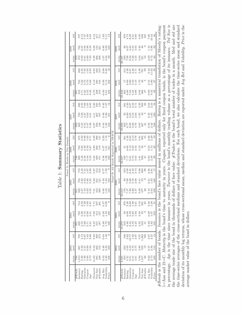
Table 1 summarizes our sample, which consists of frequently traded Phase I and II bonds
from April 2003 to June 2009. There are 1,035 bonds in our full sample, although the total
number of bonds does vary from year to year. The increase in the number of bonds from
2003 to 2004 could be a result of how NASD starts its coverage of Phase III bonds, while
the gradual reduction of number of bonds from 2004 through 2009 is a result of matured or
retired bonds.
The bonds in our sample are typically large, with a median issuance size of $750 million,
and the representative bonds in our sample are investment grade, with a median rating of 6,
which translates to Moody’s A2. The average maturity is close to 6 years and the average
6This includes cleaning up withdrawn or corrected trades, dropping trades with special sale conditions orspecial prices, and correcting for obviously mis-reported prices.
5
Tab
le1:
Sum
mary
Sta
tist
ics
PanelA
:B
onds
inO
ur
Sam
ple
2003
2004
2005
2006
2007
2008
2009
mean
med
std
mean
med
std
mean
med
std
mean
med
std
mean
med
std
mean
med
std
mean
med
std
#B
onds
744
951
911
748
632
501
373
Issu
ance
1,0
13
987
735
930
750
714
930
750
719
909
750
675
909
750
690
918
750
690
972
750
737
Rati
ng
5.3
65.2
22.1
35.5
55.0
82.3
25.6
75.0
02.4
05.3
85.0
02.3
05.3
35.0
02.3
55.7
15.9
22.3
56.6
06.6
72.1
3M
atu
rity
7.3
85.2
16.8
77.6
85.1
67.2
87.1
94.6
27.3
16.5
84.3
66.9
86.5
44.2
77.0
66.2
53.7
57.0
56.6
13.6
67.3
7C
oupon
5.8
46.0
01.6
35.7
16.0
01.6
95.6
35.8
01.6
75.4
45.5
01.6
55.4
75.6
21.6
55.5
55.7
01.6
55.8
05.8
81.6
0A
ge
2.7
31.9
42.6
83.2
12.4
12.9
13.9
33.2
52.9
04.5
23.8
72.7
15.4
64.6
12.8
36.4
25.6
62.9
37.2
36.5
03.0
3
Turn
over
11.8
38.5
29.8
39.4
77.0
97.7
17.5
15.9
25.8
75.8
34.9
93.9
94.8
74.1
13.2
64.7
04.1
92.8
35.9
85.0
64.1
2Trd
Siz
e585
462
469
557
415
507
444
331
412
409
306
366
356
267
335
248
180
240
206
134
217
#Tra
des
248
153
372
187
127
201
209
121
316
151
110
121
148
107
129
219
144
219
408
221
511
Avg
Ret
0.5
20.3
60.6
40.4
00.3
00.5
70.0
00.1
60.7
70.3
80.3
70.2
90.4
40.4
60.4
5-0
.40
0.3
62.8
91.0
70.8
01.8
3Vola
tility
2.4
92.2
51.4
81.7
21.5
90.9
81.6
21.2
41.3
91.2
81.0
11.1
81.3
91.0
81.0
75.6
13.1
48.2
24.9
43.0
95.1
1Pri
ce
108
109
9106
106
9104
103
9102
101
9103
101
12
102
102
16
99
102
13
PanelB
:A
llB
onds
Report
ed
inT
RA
CE
2003
2004
2005
2006
2007
2008
2009
mean
med
std
mean
med
std
mean
med
std
mean
med
std
mean
med
std
mean
med
std
mean
med
std
#B
onds
4,1
61
15,2
70
23,4
15
22,6
27
23,6
40
23,4
42
20,1
67
Issu
ance
453
250
540
210
50
378
176
30
353
193
31
361
203
25
391
203
17
415
239
26
470
Rati
ng
5.3
15.0
02.6
26.4
66.0
03.2
67.3
77.0
04.0
07.1
76.0
04.2
66.7
76.0
04.2
06.8
06.0
04.3
67.9
66.6
74.7
4M
atu
rity
8.5
14.5
510.7
78.3
45.3
98.8
87.8
65.0
68.4
18.0
15.1
28.6
58.0
85.0
58.9
77.8
44.8
08.8
78.0
44.8
48.9
9C
oupon
6.5
16.7
51.6
95.7
65.8
51.9
65.8
05.7
02.1
65.7
45.6
22.1
35.6
05.5
52.1
65.2
45.5
02.4
65.2
65.5
52.5
1A
ge
4.6
13.7
53.8
73.2
51.8
23.6
13.3
72.0
03.7
43.6
52.4
43.7
83.7
82.8
43.7
13.8
83.1
63.7
14.2
53.6
43.8
0
Turn
over
5.6
03.8
05.6
74.5
62.5
05.5
33.6
92.4
13.8
83.4
12.1
63.8
13.0
51.9
53.3
92.8
21.7
03.2
03.6
42.2
04.0
9Trd
Siz
e1,0
17
532
1,2
63
534
59
991
477
55
869
509
58
905
487
49
899
386
46
761
321
48
638
#Tra
des
66
19
185
31
985
26
689
21
555
21
566
27
599
54
9185
Avg
Ret
0.6
20.3
74.0
70.4
90.2
82.5
60.1
00.2
12.2
60.8
40.5
32.0
60.3
50.4
52.0
2-0
.89
0.1
56.4
22.6
91.4
47.8
6Vola
tility
2.7
32.3
62.2
71.9
21.6
71.2
92.6
41.9
32.8
12.3
01.7
42.2
92.4
21.9
52.2
49.3
25.8
011.0
29.7
25.8
610.4
4Pri
ce
109
110
12
105
103
21
100
100
17
99
99
19
100
100
34
92
97
30
84
92
46
#Bon
dsis
the
num
ber
ofbo
nds.
Issu
ance
isth
ebo
nd’s
face
valu
eis
sued
inm
illio
nsof
dolla
rs.
Rat
ing
isa
num
eric
altr
ansl
atio
nof
Moo
dy’s
rating
:1=
Aaa
and
21=
C.M
atur
ity
isth
ebo
nd’s
tim
eto
mat
urity
inye
ars.
Cou
pon,
repo
rted
only
for
fixed
coup
onbo
nds,
isth
ebo
nd’s
coup
onpa
ymen
tin
perc
enta
ge.
Age
isth
etim
esi
nce
issu
ance
inye
ars.
Tur
nove
ris
the
bond
’sm
onth
lytr
adin
gvo
lum
eas
ape
rcen
tage
ofits
issu
ance
.Trd
Size
isth
eav
erag
etr
ade
size
ofth
ebo
ndin
thou
sand
sof
dolla
rsof
face
valu
e.#
Tra
des
isth
ebo
nd’s
tota
lnu
mbe
rof
trad
esin
am
onth
.M
edan
dst
dar
eth
etim
e-se
ries
aver
ages
ofth
ecr
oss-
sect
iona
lm
edia
nsan
dst
anda
rdde
viat
ions
.Fo
rea
chbo
nd,
we
also
calc
ulat
eth
eti
me-
seri
esm
ean
and
stan
dard
devi
atio
nof
its
mon
thly
log
retu
rns,
who
secr
oss-
sect
iona
lmea
n,m
edia
nan
dst
anda
rdde
viat
ion
are
repo
rted
unde
rA
vgRet
and
Vol
atili
ty.
Pri
ceis
the
aver
age
mar
ket
valu
eof
the
bond
indo
llars
.
6

age is about 4 years. Over time, we see a gradual reduction in maturity and increase in age.
This can be attributed to our sample selection which excludes bonds issued after February 7,
2005, the beginning of Phase III.7
Given our selection criteria, the bonds in our sample are more frequently traded than
a typical bond. The average monthly turnover — the bond’s monthly trading volume as a
percentage of its issuance size — is 7.51%, the average number of trades in a month is 208.
The median trade size is $324,000. For the the whole sample in TRACE, the average monthly
turnover is 3.71%, the average number of trades in a month is 33 and the median trade size
is $65,000. Thus, the bonds in our sample are also relatively more liquid. Given that our
focus is to study the significance of illiquidity for corporate bonds, such a bias in our sample
towards more liquid bonds, although not ideal, will only help to strengthen our results if they
show up for the most liquid bonds.
In addition to the TRACE data, we use CRSP to obtain stock returns for the market and
the respective bond issuers. We use FISD to obtain bond-level information such as issue date,
issuance size, coupon rate, and credit rating, as well as to identify callable, convertible and
putable bonds. We use Bloomberg to collect the quoted bid-ask spreads for the bonds in our
sample, from which we have data for 1,032 out of the 1,035 bonds in our sample.8 We use
Datastream to collect Barclays Bond indices to calculate the default spread and returns on the
aggregate corporate bond market and also to gather CDS spreads. To calculate yield spreads
for individual corporate bonds, we obtain Treasury bond yields from the Federal Reserve,
which publishes constant maturity Treasury rates for a range of maturities. Finally, we obtain
the VIX index from CBOE.
3 Measure of Illiquidity and Its Properties
3.1 Measuring Illiquidity
Although a precise definition of illiquidity and its quantification will depend on a specific
model, two properties are clear. First, illiquidity arises from market frictions, such as costs
and constraints for trading and capital flows; second, its impact to the market is transitory.
7We will discuss later the effect, if any, of this sample selection on our results. An alternative treatmentis to include in our sample those newly issued bonds that meet the Phase II criteria, but this is difficult toimplement since the Phase II criteria are not precisely specified by FINRA.
8We follow Chen, Lesmond, and Wei (2007) in using the Bloomberg Generic (BGN) bid-ask spread. Thisspread is calculated using a proprietary formula which uses quotes provided to Bloomberg by a proprietarylist of contributors. These quotes are indicative rather than binding.
7

Thus, we construct a measure of illiquidity that is motivated by these two properties.
As such, the focus, as well as the contribution, of our paper is mainly empirical. To
facilitate our analysis, however, let us think in terms of the following simple model. Let Pt
denote the clean price — the full value minus accrued interest since the last coupon date —
of a bond at time t, and pt = ln Pt denote the log price. We start by assuming that pt consists
of two components:
pt = ft + ut . (1)
The first component ft represents its fundamental value — the log price in the absence of
frictions, which follows a random walk; the second component ut comes from the impact
of illiquidity, which is transitory (and uncorrelated with the fundamental value).9 In such
a framework, the magnitude of the transitory price component ut characterizes the level of
illiquidity in the market. γ is aimed at extracting the transitory component in the observed
price pt. Specifically, let Δpt = pt − pt−1 be the price change from t − 1 to t. We define the
measure of illiquidity γ by
γ = −Cov (Δpt, Δpt+1) . (2)
With the assumption that the fundamental component ft follows a random walk, γ depends
only on the transitory component ut, and it increases with the magnitude of ut.
Several comments are in order before we proceed with our empirical analysis of γ. First, we
know little about the dynamics of ut, other than its transitory nature. For example, when ut
follows an AR(1) process, we have γ = (1−ρ)σ2/(1+ρ), where σ is the instantaneous volatility
of ut, and 0 ≤ ρ < 1 is its persistence coefficient. In this case, while γ does provide a simple
gauge of the magnitude of ut, it combines various aspects of ut (e.g., σ and ρ). Second, for the
purpose of measuring illiquidity, other aspects of ut that are not fully captured by γ may also
matter. In other words, γ itself gives only a partial measure of illiquidity. Third, given the
potential richness in the dynamics of ut, γ will in general depend on the horizon over which
we measure price changes. This horizon effect is important because γ measured over different
horizons may capture different aspects of ut or illiquidity. For most of our analysis, we will
9Such a separation assumes that the fundamental value ft carries no time-varying risk premium. This isa reasonable assumption over short horizons. It is equivalent to assuming that high frequency variations inexpected returns are ultimately related to market frictions — otherwise, arbitrage forces would have driventhem away. To the extent that illiquidity can be viewed as a manifestation of these frictions, price movementsgiving rise to high frequency variations in expected returns should be included in ut. Admittedly, a moreprecise separation of ft and ut must rely on a pricing theory incorporating frictions or illiquidity. See, forexample, Huang and Wang (2009) and Vayanos and Wang (2009).
8
use either trade-by-trade prices or end of the day prices in estimating γ. Consequently, our γ
estimate captures more of the high frequency components in transitory price movements.
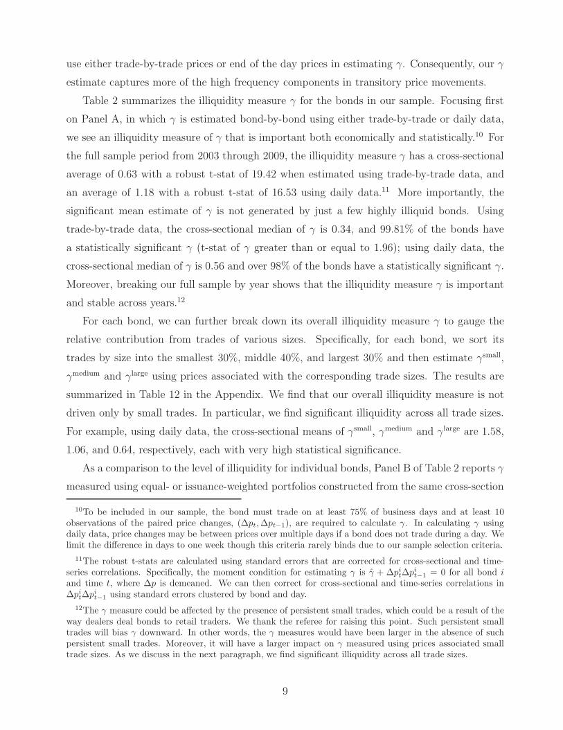
Table 2 summarizes the illiquidity measure γ for the bonds in our sample. Focusing first
on Panel A, in which γ is estimated bond-by-bond using either trade-by-trade or daily data,
we see an illiquidity measure of γ that is important both economically and statistically.10 For
the full sample period from 2003 through 2009, the illiquidity measure γ has a cross-sectional
average of 0.63 with a robust t-stat of 19.42 when estimated using trade-by-trade data, and
an average of 1.18 with a robust t-stat of 16.53 using daily data.11 More importantly, the
significant mean estimate of γ is not generated by just a few highly illiquid bonds. Using
trade-by-trade data, the cross-sectional median of γ is 0.34, and 99.81% of the bonds have
a statistically significant γ (t-stat of γ greater than or equal to 1.96); using daily data, the
cross-sectional median of γ is 0.56 and over 98% of the bonds have a statistically significant γ.
Moreover, breaking our full sample by year shows that the illiquidity measure γ is important
and stable across years.12
For each bond, we can further break down its overall illiquidity measure γ to gauge the
relative contribution from trades of various sizes. Specifically, for each bond, we sort its
trades by size into the smallest 30%, middle 40%, and largest 30% and then estimate γsmall,
γmedium and γlarge using prices associated with the corresponding trade sizes. The results are
summarized in Table 12 in the Appendix. We find that our overall illiquidity measure is not
driven only by small trades. In particular, we find significant illiquidity across all trade sizes.
For example, using daily data, the cross-sectional means of γsmall, γmedium and γlarge are 1.58,
1.06, and 0.64, respectively, each with very high statistical significance.
As a comparison to the level of illiquidity for individual bonds, Panel B of Table 2 reports γ
measured using equal- or issuance-weighted portfolios constructed from the same cross-section
10To be included in our sample, the bond must trade on at least 75% of business days and at least 10observations of the paired price changes, (Δpt, Δpt−1), are required to calculate γ. In calculating γ usingdaily data, price changes may be between prices over multiple days if a bond does not trade during a day. Welimit the difference in days to one week though this criteria rarely binds due to our sample selection criteria.
11The robust t-stats are calculated using standard errors that are corrected for cross-sectional and time-series correlations. Specifically, the moment condition for estimating γ is γ̂ + Δpi
tΔpit−1 = 0 for all bond i
and time t, where Δp is demeaned. We can then correct for cross-sectional and time-series correlations inΔpi
tΔpit−1 using standard errors clustered by bond and day.
12The γ measure could be affected by the presence of persistent small trades, which could be a result of theway dealers deal bonds to retail traders. We thank the referee for raising this point. Such persistent smalltrades will bias γ downward. In other words, the γ measures would have been larger in the absence of suchpersistent small trades. Moreover, it will have a larger impact on γ measured using prices associated smalltrade sizes. As we discuss in the next paragraph, we find significant illiquidity across all trade sizes.
9

of bonds and for the same sample period. In contrast to its counterpart at the individual bond
level, γ at the portfolio level is slightly negative, rather small in magnitude, and statistically
insignificant. This implies that the transitory component extracted by the γ measure is
idiosyncratic in nature and gets diversified away at the portfolio level. It does not imply,
however, that the illiquidity in corporate bonds lacks a systematic component, which we will
examine later in Section 3.3.
Table 2: Measure of Illiquidity γ = −Cov (pt − pt−1, pt+1 − pt)
Panel A: Individual Bonds2003 2004 2005 2006 2007 2008 2009 Full
Trade-by-Trade DataMean γ 0.64 0.60 0.52 0.40 0.44 1.02 1.35 0.63Median γ 0.41 0.32 0.25 0.19 0.24 0.57 0.63 0.34Per t ≥ 1.96 99.46 98.64 99.34 99.87 99.69 98.80 97.98 99.81Robust t-stat 14.54 16.22 15.98 15.12 14.88 12.58 9.45 19.42
Daily DataMean γ 0.99 0.82 0.77 0.57 0.80 3.21 5.40 1.18Median γ 0.61 0.41 0.34 0.29 0.47 1.36 1.94 0.56Per t ≥ 1.96 94.62 92.64 95.50 96.26 95.57 95.41 97.59 98.84Robust t-stat 17.28 17.88 18.21 19.80 14.39 7.16 8.47 16.53
Panel B: Bond Portfolios2003 2004 2005 2006 2007 2008 2009 Full
Equal-weighted -0.0014 -0.0043 -0.0008 0.0001 0.0023 -0.0112 -0.0301 -0.0050t-stat -0.29 -1.21 -0.47 0.11 1.31 -0.26 -2.41 -0.71Issuance-weighted 0.0018 -0.0042 -0.0003 0.0007 0.0034 0.0030 -0.0280 -0.0017t-stat 0.30 -1.14 -0.11 0.41 1.01 0.06 -1.97 -0.20
Panel C: Implied by Quoted Bid-Ask Spreads2003 2004 2005 2006 2007 2008 2009 Full
Mean implied γ 0.035 0.031 0.034 0.028 0.031 0.050 0.070 0.034Median implied γ 0.031 0.025 0.023 0.018 0.021 0.045 0.059 0.026
At the individual bond level, γ is calculated using either trade-by-trade or daily data. Per t-stat ≥ 1.96reports the percentage of bond with statistically significant γ. Robust t-stat is a test on the cross-sectionalmean of γ with standard errors corrected for cross-sectional and time-series correlations. At the portfoliolevel, γ is calculated using daily data and the Newey-West t-stats are reported. Monthly quoted bid-askspreads, which we have data for 1,032 out of 1,035 bonds in our sample, are used to calculate the impliedγ.
Panel C of Table 2 provides another and perhaps more important gauge of the magnitude
of our estimated γ for individual bonds. Using quoted bid-ask spreads for the same cross-
section of bonds and for the same sample period, we estimate a bid-ask implied γ for each
bond by computing the magnitude of negative autocovariance that would have been generated
by bid-ask bounce. For the full sample period, the cross-sectional mean of the implied γ is
0.034 and the median is 0.026, which are more than one order of magnitude smaller than the
10

empirically observed γ for individual bonds. As shown later in the paper, not only does the
quoted bid-ask spread fail to capture the overall level of illiquidity, but it also fails to explain
the cross-sectional variation in bond illiquidity and its asset pricing implications.
Although our focus is on extracting the transitory component at the trade-by-trade and
daily frequencies, it is interesting to provide a general picture of γ over varying horizons. Mov-
ing from the trade-by-trade to daily horizon, our results in Table 2 show that the magnitude
of the illiquidity measure γ becomes larger. Given that the autocovariance at the daily level
cumulatively captures the mean-reversion at the trade-by-trade level, this implies that the
mean-reversion at the trade-by-trade level persists for a few trades before fully dissipating,
which we show in Section 6.1. Moving from the daily to weekly horizon, we find that the
magnitude of γ increases slightly from an average level of 1.18 to 1.21, although its statisti-
cal significance decreases to a robust t-stat of 14.16, and 77.88% of the bonds in our sample
have a positive and statistically significant γ at this horizon. Extending to the bi-weekly and
monthly horizons, γ starts to decline in both magnitude and statistical significance.13
As mentioned earlier in the section, the transitory component ut might have richer dy-
namics than what can be offered by a simple AR(1) structure for ut. By extending γ over
various horizons, we are able to uncover some of the dynamics. We show in Section 6.1 that
at the trade-by-trade level ut is by no means a simple AR(1). Likewise, in addition to the
mean-reversion at the daily horizon that is captured in this paper, the transitory component
ut may also have a slow moving mean-reversion component at a longer horizon. To examine
this issue more thoroughly is an interesting topic, but requires time-series data for a longer
sample period than ours.14
13At a bi-weekly horizon, the mean gamma is 1.16 with a t-stat of 6.37. 42.18% of the bonds have a significantgamma. At the monthly horizon, gamma is 0.80 with a t-stat of 2.02 and only 17.09% are significant. Inaddition to having fewer observations, Using longer horizons also decreases the signal to noise ratio as thefundamental volatility starts to build up. See Harris (1990) for the exact small sample moments of the serialcovariance estimator and of the standard variance estimator for price changes generated by the Roll spreadmodel.
14By using monthly bid prices from 1978 to 1998, Khang and King (2004) report contrarian patterns incorporate bond returns over horizons of one to six months. Instead of examining autocovariance in bondreturns, their focus is on the cross-sectional effect. Sorting bonds by their past monthly (or bi-monthly up to6 months) returns, they find that past winners under perform past losers in the next month (or 2-month upto 6 months). Their result, however, is relatively weak and is significant only in the early half of their sampleand goes away in the second half of their sample (1988–1998).
11

3.2 Illiquidity and Bond Characteristics
Our sample includes a broad cross-section of bonds, which allows us to examine the connection
between the illiquidity measure γ and various bond characteristics, some of which are known
to be linked to bond liquidity. The variation in γ and bond characteristics is reported in
Table 3. We use daily data to construct yearly estimates of γ for each bond and perform
pooled regressions on various bond characteristics. Reported in square brackets are the t-
stats calculated using standard errors clustered by year.
We find that older bonds on average have higher γ, and the results are robust regardless of
which control variables are used in the regression. On average, a bond that is one-year older
is associated with an increase of 0.19 in its γ, which accounts for more than 15% of the full-
sample average of γ. Given that the age of a bond has been widely used in the fixed-income
market as a proxy for illiquidity, it is important that we establish this connection between
γ and age. Similarly, we find that bonds with smaller issuance tend to have larger γ. We
also find that bonds with longer time to maturity typically have higher γ. We do not find a
significant relation between credit ratings and γ, and this can be attributed to the fact that
our sample includes investment-grade bonds only.15
Given that we have transaction-level data, we can also examine the connection between γ
and bond trading activity. We find that, by far, the most interesting variable is the average
trade size of a bond. In particular, bonds with smaller trade sizes have higher illiquidity
measure γ. We also find that bonds with a larger number of trades are have higher γ and are
less liquid. In other words, more trades do not imply more liquidity, especially if these trades
are of small sizes.
To examine the connection between γ and quoted bid-ask spreads, we use quoted bid-ask
spreads to obtain bid-ask implied γ’s. We find a positive relation between our γ measure
and the γ measure implied by the quoted bid-ask spread. It is interesting to point out,
however, that adding the bid-ask implied γ as an explanatory variable does not alter the
relation between our γ measure and liquidity-related bond characteristics such as age and
size. Overall, we find that the magnitude of illiquidity captured by our γ measure is related
to but goes beyond the information contained in the quoted bid-ask spreads.
Finally, given the extent of CDS activity during our sample period and its close relation
with the corporate bond market, it is also interesting for us to explore the connection between
15In our earlier analysis that includes both investment-grade and junk bonds, we do find that γ is higherfor lower graded bonds.
12
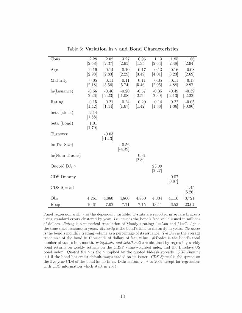
Table 3: Variation in γ and Bond Characteristics
Cons 2.28 2.02 3.27 0.95 1.13 1.85 1.86[2.58] [2.37] [2.95] [1.35] [2.64] [2.48] [2.94]
Age 0.19 0.14 0.10 0.17 0.13 0.16 0.08[2.98] [2.83] [2.29] [3.49] [4.01] [3.23] [2.69]
Maturity 0.05 0.11 0.11 0.11 0.05 0.11 0.13[2.18] [5.56] [5.74] [5.46] [2.95] [4.88] [2.97]
ln(Issuance) -0.56 -0.46 -0.20 -0.57 -0.35 -0.49 -0.39[-2.26] [-2.23] [-1.08] [-2.59] [-2.39] [-2.13] [-2.22]
Rating 0.15 0.21 0.24 0.20 0.14 0.22 -0.05[1.42] [1.44] [1.67] [1.42] [1.38] [1.36] [-0.96]
beta (stock) 2.14[1.88]
beta (bond) 1.01[1.79]
Turnover -0.03[-1.13]
ln(Trd Size) -0.56[-4.39]
ln(Num Trades) 0.31[2.89]
Quoted BA γ 23.09[2.27]
CDS Dummy 0.07[0.87]
CDS Spread 1.45[5.26]
Obs 4,261 4,860 4,860 4,860 4,834 4,116 3,721R-sqd 10.61 7.02 7.71 7.15 13.11 6.53 23.07
Panel regression with γ as the dependent variable. T-stats are reported in square bracketsusing standard errors clustered by year. Issuance is the bond’s face value issued in millionsof dollars. Rating is a numerical translation of Moody’s rating: 1=Aaa and 21=C. Age isthe time since issuance in years. Maturity is the bond’s time to maturity in years. Turnoveris the bond’s monthly trading volume as a percentage of its issuance. Trd Size is the averagetrade size of the bond in thousands of dollars of face value. #Trades is the bond’s totalnumber of trades in a month. beta(stock) and beta(bond) are obtained by regressing weeklybond returns on weekly returns on the CRSP value-weighted index and the Barclays USbond index. Quoted BA γ is the γ implied by the quoted bid-ask spreads. CDS Dummyis 1 if the bond has credit default swaps traded on its issuer. CDS Spread is the spread onthe five-year CDS of the bond issuer in %. Data is from 2003 to 2009 except for regressionswith CDS information which start in 2004.
13

γ and information from the CDS market. We find two interesting results. First, we find that
whether or not a bond issuer has CDS traded on it does not affect the bond’s liquidity. Given
that our sample includes only investment-grade bonds and over 90% of the bond-years in our
sample have traded CDS, this result is hardly surprising. Second, we find that, within the
CDS sample, bonds with higher CDS spreads have significantly higher γ’s and are therefore
less liquid. This implies that even at the name issuer level, there is a close connection between
credit and liquidity risks. We now move on to the aggregate level to examine whether or not
this liquidity risk has a systematic component and explores its relation with the systematic
credit risk.
3.3 Aggregate Illiquidity and Market Conditions
Next, we examine how the illiquidity of corporate bonds varies over time. Instead of con-
sidering individual bonds, we are more interested in the comovement in their illiquidity. For
this purpose, we construct an aggregate measure of illiquidity using the bond-level illiquidity
measure. We first construct, with a monthly frequency, a cross-section of γ’s for all individual
bonds using daily data within that month.16 We then use the cross-sectional median γ as the
aggregate γ measure.17 If the bond-level illiquidity we have documented so far is purely driven
by idiosyncratic reasons, then we would not expect to see any interesting time-series variation
of this aggregate γ measure. In other words, the systematic component of bond illiquidity can
only emerge when many bonds become illiquid around the same time.
From Figure 1, we see that there is indeed a substantial level of commonality in the
bond-level illiquidity, indicating a rather important systematic illiquidity component. More
importantly, this aggregate illiquidity measure comoves strongly with the aggregate market
condition at the time. The 2008 sub-prime crisis is perhaps the most prominent event in our
sample. Before August 2007, the aggregate γ was hovering around an average level of 0.30
with a standard deviation of 0.10. In August 2007, when the credit crisis first broke out, the
aggregate γ doubled to a level of 0.60, and in March 2008, during the collapse of Bear Stearns,
16In calculating the monthly autocovariance of price changes, we can demean the price change using thesample mean within the month, within the year, or over the entire sample period. It depends on whether weview the monthly variation in the mean of price change as noise or as some low-frequency movement related tothe fundamental. In practice, however, this time variation is rather small compared with the high-frequencybouncing around the mean. As a result, demeaning using the monthly mean or the sample mean generatesvery similar results. Here we report the results using the former.
17Compared with the cross-sectional mean of γ, the median γ is a more conservative measure and is lesssensitive to those highly illiquid bonds that were most severely affected by the credit market turmoil.
14

2003 2004 2005 2006 2007 2008 2009 20100
0.5
1
1.5
2
2.5
3
3.5
Gam
ma
May 2005 Aug 2007
Sept 2008
Mar 2008
2003 2004 2005 2006 2007 2008 2009 20100.2
0.3
0.4
0.5
0.6
0.7
0.8
0.9
Gam
ma
Pre−2008
May 2005Dec 2007
Aug 2007
Figure 1: Monthly time-series of aggregate illiquidity. The top panel is for the whole sample,and the bottom panel focuses on the pre-2008 period.
15

the aggregate γ jumped to a level of 0.90, which tripled the pre-crisis average and was the
all-time high at that point. In September 2008, during the Lehman default and the bailout of
AIG , we see the aggregate γ reaching 1.59, which was over 12 standard deviations away from
its pre-crisis level. The aggregate γ peaked in October 2008 at 3.37, indicating a worsening
liquidity situation after the Lehman/AIG event. After the peak illiquidity in October 2008,
we see a slow but steady improvement of liquidity, which coincided with the liquidity injection
provided by Fed and the improved condition of the overall market.18
The connection between the aggregate γ and broader market conditions indicates that
although it is constructed using only corporate bond data, the aggregate illiquidity captured
here seems to have a wider reach than this particular market. Indeed, as reported in Table 4,
regressing monthly changes in aggregate γ on contemporaneous changes in the CBOE VIX
index, we obtain a slope coefficient of 0.0468 with a t-stat of 6.45, and the R-squared of
the OLS regression is over 67%. This result is not driven just by the 2008 sub-prime crisis:
excluding data from 2008 and 2009, the positive relation is still robust: the slope coefficient
is 0.0162 with a t-stat of 2.87 and the R-squared is 33%.
The fact that the aggregate illiquidity measure γ has a close connection with the VIX index
is a rather intriguing result. While one measure is captured from the trading of individual
corporate bonds, to gauge the overall liquidity condition of the market, the other is captured
from the pricing of the S&P 500 index options, often referred to as the “fear gauge” of the
market. Our result seems to indicate that there is a non-trivial interaction between shocks to
market illiquidity and shocks to market risk and/or risk appetite.
Also reported in Table 4 are the relation between the aggregate γ and other market-
condition variables. As a proxy for the overall credit risk, we consider an average CDS
index, constructed as the average of five-year CDS spreads covered by CMA Datavision in
Datastream.19 We find a weak positive relation between changes in aggregate γ and changes in
18By focusing only on Phase I and II bonds in TRACE to maintain a reasonably balanced sample, we didnot include bonds that were included only after Phase III, which was fully implemented on February 7, 2005.Consequently, new bonds issued after that date were excluded from our sample, even though some of themwould have been eligible for Phase II had they been issued earlier. As a result, starting from February 7, 2005,we have a population of slowly aging bonds. Since γ is positively related to age, it might introduce a slightoverall upward trend in γ. It should be mentioned that the sudden increases in aggregate γ during crises aretoo large to be explained by the slow aging process. Finally, to avoid regressing trend on trend, the time-seriesregression results presented later in this section are based on regressing changes on changes. we also did arobustness check by constructing a subsample of bonds with less of the aging effect, and our time-series resultsin this section remain the same.
19For robustness, we also consider a CDS index using only the subset of names that correspond to the bondsin our sample and find similar results.
16
the CDS index. Interestingly, if we exclude 2008 and 2009, the connection between the two is
stronger. We also find that lagged bond returns are negatively related to changes in aggregate
γ, indicating that, on average, negative bond market performance is followed by worsening
liquidity conditions. Putting VIX into these regressions, however, these two variables become
insignificant. The one market condition variable that is significant after controlling for VIX
is the volatility of the Barclays US Investment Grade Corporate Bond Index, but this is only
true if crisis period data is included.
Table 4: Time Variation in Aggregate γ and Market Variables
Panel A: Full SampleCons 0.0003 0.0036 -0.0027 0.0020 0.0061 0.0078 0.0096 0.0014
[0.03] [0.13] [-0.15] [0.07] [0.21] [0.27] [0.40] [0.12]Δ VIX 0.0468 0.0497
[6.45] [3.58]Δ Bond Volatility 0.0411 0.0303
[1.82] [2.92]Δ CDS Index 0.2101 -0.0408
[1.91] [-0.64]Δ Term Spread 0.3610
[1.01]Δ Default Spread -0.0038
[-0.04]Lagged Stock Return -0.0082
[-0.94]Lagged Bond Return -0.0506 0.0039
[-2.35] [0.17]Adj R-sqd (%) 67.47 3.31 12.77 6.38 -1.41 0.46 13.57 70.01
Panel B: 2003 - 2007 OnlyCons 0.0012 0.0018 0.0014 0.0050 0.0011 0.0116 0.0029 0.0128
[0.19] [0.21] [0.32] [0.60] [0.19] [1.22] [0.36] [2.42]Δ VIX 0.0162 0.0108
[2.87] [2.21]Δ Bond Volatility -0.0038
[-0.43]Δ CDS Index 0.3640 0.1213
[2.94] [1.51]Δ Term Spread 0.1204 0.1020
[2.76] [2.87]Δ Default Spread 0.2362
[1.35]Lagged Stock Return -0.0103 -0.0068
[-3.27] [-2.74]Lagged Bond Return -0.0127 -0.0039
[-4.22] [-0.94]Adj R-sqd (%) 33.11 -1.51 37.76 8.87 10.82 18.00 6.98 55.11
Monthly changes in γ regressed on monthly changes in bond index volatility, VIX, CDS index, term spread,default spread, and lagged stock and bond returns. The Newey-West t-stats are reported in square brackets.Regressions with CDS Index do not include 2003 data.
17

The analysis above leads to three conclusions. First, there is substantial commonality
in the time variation of corporate bond illiquidity. Second, this time variation is correlated
with overall market conditions. Third, changes in the aggregate γ exhibits strong positive
correlation with changes in VIX.
4 Illiquidity and Bond Yields
After having established the empirical properties of the illiquidity measure γ, we now explore
the connections between illiquidity and corporate bond pricing. In particular, we examine the
extent to which illiquidity affects pricing, in both the time-series and the cross-section.
4.1 Aggregate Illiquidity and Aggregate Bond Yield Spreads
We use the Barclays US Corporate Bond Indices (formerly known as the Lehman Indices) to
measure aggregate bond yield spreads of various ratings. We regress monthly changes in the
aggregate bond yield spreads on monthly changes in the aggregate illiquidity measure γ and
other market-condition variables. The results are reported in Table 5.
We find that the aggregate γ plays an important role in explaining the monthly changes
in the aggregate yield spreads. This is especially true for ratings A and above, where the
aggregate γ is by far the most important variable, explaining over 51% of the monthly variation
in yield spreads for AAA-rated bonds, 47% for AA-rated bonds, and close to 60% for A-rated
bonds. Adding the CDS index as a proxy for credit risk, we find that it also plays an important
role, but illiquidity remains the dominant factor in driving the yield spreads for ratings A and
above. On the other hand, the CBOE VIX index does not have any additional explanatory
power in the presence of the aggregate γ and the CDS index. This implies that despite their
strong correlation, the aggregate γ is far from a mere proxy for VIX. It contains important
information about bond yields while VIX does not provide any additional information.20
Overall, our results indicate that both illiquidity, as captured by the aggregate γ, and
credit risk, as captured by the CDS index, are important drivers for high-rated yield spreads.
During normal market conditions, these two components seem to carry equal importance. This
can be seen in Panel B of Table 5, where only pre-2008 data are used. During the 2008 crisis,
however, illiquidity becomes a much more important component, over-shadowing the credit
20We have done additional tests regarding the marginal information changes in the aggregate γ and VIXprovide, respectively, about changes in bond prices. When we replace changes in the aggregate γ by its residualafter an projection on changes in VIX, the residual remains significant and substantial. However, when wereplace VIX by its residual after an projection on changes in the aggregate γ, the residual is not significant.
18

Table 5: Aggregate Bond Yield Spreads and Aggregate Illiquidity
Panel A: Full Sample (2003/05-2009/06)
AAA AAA AA AA A A BAA BAA Junk JunkIntercept 0.001 -0.009 0.014 0.011 0.018 0.014 0.028 0.014 0.049 0.005
[0.05] [-0.45] [0.52] [0.58] [0.61] [0.72] [0.50] [0.76] [0.39] [0.10]Δγ 0.896 0.671 0.737 0.502 1.074 0.879 0.903 0.561 2.114 0.348
[7.75] [6.18] [5.70] [6.33] [8.55] [7.87] [3.90] [3.27] [4.22] [0.64]Δ CDS Index 0.140 0.235 0.271 0.519 1.461
[1.62] [3.72] [3.36] [4.27] [3.25]Δ VIX 0.009 -0.002 -0.006 -0.008 0.055
[0.59] [-0.26] [-0.70] [-0.77] [1.25]Δ Bond Volatility 0.051 0.020 0.014 -0.027 -0.028
[1.97] [1.71] [1.38] [-1.17] [-0.85]Δ Term Spread -0.256 -0.221 -0.166 -0.040 -0.537
[-1.56] [-1.34] [-0.83] [-0.20] [-1.11]Lagged Stock Return -0.020 -0.003 -0.009 -0.016 -0.038
[-1.37] [-0.46] [-1.20] [-2.22] [-1.18]Lagged Bond Return 0.015 -0.042 -0.037 -0.039 -0.012
[0.77] [-1.65] [-1.47] [-3.11] [-0.28]Adj R-sqd (%) 51.56 69.91 47.11 80.80 59.86 85.12 28.17 83.39 23.22 85.50
Panel B: Pre-Crisis (2003/05-2007/12)
AAA AAA AA AA A A BAA BAA Junk JunkIntercept 0.010 0.019 0.021 0.027 0.016 0.033 0.011 0.028 -0.003 0.008
[1.19] [1.42] [1.54] [1.88] [1.01] [1.76] [0.63] [1.30] [-0.08] [0.22]Δγ 0.583 0.348 0.822 0.478 0.966 0.425 1.106 0.404 3.678 -0.063
[3.87] [2.56] [2.99] [2.83] [3.47] [2.20] [3.53] [1.42] [4.67] [-0.10]Δ CDS Index 0.218 0.340 0.399 0.553 3.025
[2.32] [2.35] [2.50] [2.08] [9.85]Δ VIX -0.003 0.001 -0.002 -0.003 0.026
[-0.55] [0.11] [-0.21] [-0.30] [1.83]Δ Bond Volatility 0.011 0.023 0.019 0.025 0.013
[1.18] [1.66] [1.36] [1.45] [0.59]Δ Term Spread 0.022 -0.058 0.076 0.105 -0.112
[0.24] [-0.43] [0.50] [0.64] [-0.40]Lagged Stock Return -0.006 -0.002 -0.008 -0.005 -0.002
[-1.03] [-0.37] [-1.09] [-0.72] [-0.20]Lagged Bond Return 0.005 0.009 0.012 -0.000 0.009
[0.91] [0.84] [1.26] [-0.01] [0.39]Adj R-sqd (%) 24.93 40.82 19.42 37.74 26.88 45.64 22.44 30.09 29.40 80.25
Monthly changes in yields on Barclay’s Intermediate Term indices regressed on monthly changes in aggregateγ, aggregated % bid-ask spreads, bond index volatility, VIX, CDS index, term spread, and lagged stock andbond returns. The top row indicates the rating index used in the regression. Newey-West t-stats are reportedin square brackets. Regressions with CDS Index do not include 2003 data.
19

risk effect. This is especially true for AAA-rated bonds, whose connection to credit risk is no
longer significant when 2008 and 2009 data are included.21 At the same time, its connection
to illiquidity increases rather significantly. In particular, in the univariate regression, the
R-squared doubles from 25% to 52% when 2008 and 2009 are included. Pre-crisis, a one
standard deviation increase in monthly changes in aggregate γ (which is 0.06) results in a
3.5 bps increase in yield spreads for AAA-rated bonds. After including 2008 and 2009, a one
standard deviation increase in monthly changes in aggregate γ (which is 0.27) results in a 24
bps increase in yield spreads.
Applying this observation to the debate of whether the 2008 crisis was a liquidity or credit
crisis, our results seem to indicate that as far as high-rated corporate bonds are concerned,
the sudden increase in aggregate illiquidity was a dominating force in driving up the yield
spreads.
Our results also show that while aggregate illiquidity issue plays an important role in
explaining the monthly changes in yield spreads for high-rated bonds, it is less important for
junk bonds. For such bonds, credit risk is a more important component. This does not mean
that junk bonds are more liquid. In fact, they are generally less liquid. Given the low credit
quality of such bonds, however, they are more sensitive to the overall credit condition than
the overall illiquidity condition. This is also consistent with the findings of Huang and Huang
(2003). Pricing corporate bonds using structural models of default, they find that, for the
low-rated bonds, a large portion of their yield spreads can be explained by credit risk, while
for high-rated bonds, credit risk can explain only a tiny portion of their yield spreads.
4.2 Bond-Level Illiquidity and Individual Bond Yield Spreads
We now examine how bond-level γ can help to explain the cross section of bond yields. For
this purpose, we focus on the yield spread of individual bonds, which is the difference between
the corporate bond yield and the Treasury bond yield of the same maturity. For Treasury
yields, we use the constant maturity rate published by the Federal Reserve and use linear
interpolation whenever necessary. We perform monthly cross-sectional regressions of the yield
spreads on the illiquidity measure γ, along with a set of control variables.
The results are reported in Table 6, where the t-stats are calculated using the Fama-
MacBeth standard errors with serial correlation corrected using Newey and West (1987). To
21We construct the CDS index using all available CDS data from CMA in Datastream. For robustness, wefurther construct a CDS index using only CDS’s on the firms in our sample. The results are similar and ourmain conclusions in this subsection are robust to both measures of CDS indices.
20

include callable bonds in our analysis, which constitute a large portion of our sample, we use
a callable dummy, which is one if a bond is callable and zero otherwise.22 We exclude all
convertible and putable bonds from our analysis. In addition, we also include rating dummies
for A and Baa. The first column in Table 6 shows that (controlling for callability), the average
yield spread of the Aaa and Aa bonds in our sample is 129 bps, relative to which the A bonds
are 61 bps higher, and Baa bonds are 176 bps higher.
As reported in the second column of Table 6, adding γ to the regression does not bring
much change to the relative yield spreads across ratings. This is to be expected since γ should
capture more of a liquidity effect, and less of a fundamental risk effect, which is reflected in
the differences in ratings. More importantly, we find that the coefficient on γ is 0.17 with
a t-stat of 9.60. This implies that for two bonds in the same rating category, if one bond,
presumably less liquid, has a γ that is higher than the other by 1, the yield spread of this
bond is on average 17 bps higher than the other. To put an increase of 1 in γ in context, the
cross-sectional standard deviation of γ is on average 2.03 in our sample. From this perspective,
the illiquidity measure γ is economically important in explaining the cross-sectional variation
in average bond yields.
To control for the fundamental risk of a bond above and beyond what is captured by the
rating dummies, we use equity volatility estimated using daily equity returns of the bond
issuer. Effectively, this variable is a combination of the issuer’s asset volatility and leverage.
We find this variable to be important in explaining yield spreads. As shown in the third
column of Table 6, the slope coefficient on equity volatility is 0.02 with a t-stat of 3.36. That
is, a ten percentage point increase in the equity volatility of a bond issuer is associated with a
20 bps increase in the bond yield. While adding γ improves the cross-sectional R-squared from
a time-series average of 19.00% to 30.27%, adding equity volatility improves the R-squared
to 25.97%. Such R-squareds, however, should be interpreted with caution since it is a time-
series average of cross-sectional R-squared, and does not take into account the cross-sectional
correlations in the regression residuals. By contrast, our reported Fama-MacBeth t-stats do
and γ has a stronger statistical significance. It is also interesting to observe that by adding
equity volatility, the magnitudes of the rating dummies decrease significantly. This is to be
expected since both equity volatility and rating dummies are designed to control for the bond’s
fundamental risk.
When used simultaneously to explain the cross-sectional variation in bond yield spreads,
22In the Appendix, we also report results with callable bonds excluded.
21

Tab
le6:
Bond
Yie
ldSpre
ad
and
Illiquid
ity
Measu
reγ
Con
s1.
291.
130.
330.
300.
560.
460.
230.
580.
04-0
.00
1.18
0.34
0.62
[3.6
6][3
.60]
[2.3
1][2
.86]
[8.3
6][2
.43]
[1.4
1][3
.24]
[0.1
6][-0
.02]
[2.4
8][3
.26]
[3.6
2]γ
0.17
0.16
0.12
0.09
0.10
0.08
0.09
0.09
0.15
0.10
[9.6
0][8
.75]
[6.6
9][6
.21]
[6.2
2][5
.85]
[6.1
4][6
.30]
[10.
33]
[7.7
2]E
quity
Vol
0.02
0.02
-0.0
00.
020.
020.
020.
010.
020.
02-0
.00
[3.3
6][3
.61]
[-0.6
3][3
.69]
[3.5
0][3
.87]
[3.1
6][3
.61]
[3.7
4][-0
.51]
CD
SSp
read
0.69
0.67
[12.
94]
[11.
08]
Age
0.01
0.02
0.00
0.01
0.01
[0.8
9][1
.76]
[0.4
5][1
.30]
[1.1
1]M
atur
ity
0.01
0.01
0.01
0.01
0.01
[0.5
9][0
.66]
[0.6
1][0
.52]
[0.6
5]ln
(Iss
uanc
e)-0
.02
-0.0
1-0
.00
-0.0
8-0
.04
[-1.2
3][-0
.44]
[-0.0
9][-3
.46]
[-1.8
7]Tur
nove
r0.
02[2
.57]
ln(T
rdSi
ze)
-0.0
4[-0
.99]
ln(#
Tra
des)
0.16
[3.4
1]%
Day
sTra
ded
0.01
[3.1
2]Q
uote
dB
/ASp
read
0.48
0.18
0.02
[1.1
7][0
.47]
[0.0
5]C
allD
umm
y-0
.67
-0.6
4-0
.17
-0.2
2-0
.08
-0.2
6-0
.24
-0.2
6-0
.23
-0.2
5-0
.71
-0.2
4-0
.08
[-1.5
6][-1
.69]
[-1.1
4][-1
.50]
[-0.6
0][-2
.05]
[-1.9
9][-2
.10]
[-1.8
4][-2
.03]
[-1.7
7][-1
.87]
[-0.7
4]A
Dum
my
0.61
0.55
0.35
0.33
0.28
0.35
0.34
0.36
0.38
0.36
0.62
0.35
0.29
[2.3
8][2
.53]
[2.7
5][3
.00]
[2.0
7][2
.87]
[2.7
8][3
.11]
[3.0
4][2
.93]
[2.3
2][2
.81]
[2.0
1]B
AA
Dum
my
1.76
1.52
1.44
1.29
0.76
1.25
1.22
1.28
1.29
1.27
1.70
1.23
0.71
[2.8
1][3
.07]
[2.9
9][3
.19]
[2.4
9][2
.97]
[2.8
9][3
.17]
[3.0
0][2
.96]
[2.7
4][3
.15]
[2.4
7]O
bs60
159
460
159
452
959
459
459
459
459
358
658
151
8R
-sqd
(%)
19.0
030
.27
25.9
735
.85
57.6
045
.07
45.9
746
.19
48.1
845
.52
26.1
439
.84
60.3
1
Mon
thly
Fam
a-M
acB
eth
cros
s-se
ctio
nalr
egre
ssio
nw
ith
the
bond
yiel
dsp
read
asth
ede
pend
ent
vari
able
.T
het-
stat
sar
ere
port
edin
squa
rebr
acke
tsca
lcul
ated
usin
gFa
ma-
Mac
Bet
hst
anda
rder
rors
with
seri
alco
rrel
atio
nco
rrec
ted
usin
gN
ewey
-Wes
t.T
here
port
ednu
mbe
rof
obse
rvat
ions
are
the
aver
age
num
ber
ofob
serv
atio
nspe
rpe
riod
.T
here
port
edR
-squ
ared
sar
eth
eti
me-
seri
esav
erag
esof
the
cros
s-se
ctio
nalR
-squ
ared
s.γ
isth
em
onth
lyes
tim
ate
ofill
iqui
dity
mea
sure
usin
gda
ilyda
ta.
Equ
ity
Vol
ises
tim
ated
usin
gda
ilyeq
uity
retu
rns
ofth
ebo
ndis
suer
.Age
,M
atur
ity,
Issu
ance
,Tur
nove
r,Trd
Size
,an
d#
Tra
des
are
asde
fined
inTab
le3.
Cal
lD
umm
yis
one
ifth
ebo
ndis
calla
ble
and
zero
othe
rwis
e.C
onve
rtib
lean
dpu
tabl
ebo
nds
are
excl
uded
from
the
regr
essi
on.
The
sam
ple
peri
odis
from
May
2003
thro
ugh
June
2009
.
22

both γ and equity volatility are significant, with the slope coefficients for both remaining
more or less the same as before. This implies a limited interaction between the two variables,
which is to be expected since the equity volatility is designed to pick up the fundamental
information about a bond while γ is to capture its liquidity information. Moreover, the
statistical significance of γ is virtually unchanged.
Taking advantage of the fact that a substantial sub-sample of our bonds have CDS traded
on their issuers, we use CDS spreads as an additional control for the fundamental risk of a
bond. We find a very strong relation between bond yields and CDS yields: the coefficient is
0.69 with a t-stat of 12.94. For the sub-sample of bonds with CDS traded, and controlling for
the CDS spread, we still find a strong cross-sectional relation between γ and bond yields. The
economic significance of the relation is smaller: a cross-sectional difference of γ of 1 translates
to a 12 bps difference in bond yields.
Given that both bond age and bond issuance are known to be linked to liquidity,23 we
add these bond characteristics as controls, and find that the positive connection between γ
and average bond yield spreads remains robust. Further adding the bond trading variables as
controls, we find these variables do not have a strong impact on the positive relation between
the illiquidity measure γ and average yield spreads.
We also examine the relative importance of the quoted bid-ask spreads and γ. As shown
in the last two columns of Table 6, the quoted bid-ask spreads are negatively related average
yield spreads. Using both the quoted bid-ask spreads and γ, we find a robust result for γ and
a statistically insignificant result for the quoted bid-ask spread. This aspect of our result is
different from that in Chen, Lesmond, and Wei (2007), who find a positive relation between the
quoted bid-ask spreads and yield spreads. This discrepancy is mainly due to the recent crisis
period. There is, in fact, a positive relation between quoted bid-ask spreads and yield spreads
before 2008. This, however, does not affect our results for γ, which remain economically and
statistically significant even if only pre-2008 data is used. Chen, Lesmond, and Wei (2007)
also use zero return days as a proxy for illiquidity.24 As zero return days are meant to be a
proxy for non-trading while we directly observe trading, we instead use the % of days with
trading. When we include this measure in the regression, it comes in significant, but with the
wrong sign.
23See, for example, Houweling, Mentink, and Vorst (2003) and additional references therein.24See Bekaert, Harvey, and Lundblad (2007) for a discussion of when the zero return measure is appropriate.
23

5 Illiquidity and Bid-Ask Spread
It is well known that the bid-ask spread can lead to negative autocovariance in price changes.
For example, using a simple specification, Roll (1984) shows that when transactions prices
bounce between bid and ask prices, depending on whether they are sell or buy orders from
customers, their changes exhibit negative autocovariance even when the “underlying value”
follows a random walk. Thus, it is important to ask whether or not the negative autoco-
variances documented in this paper are simply a reflection of bid-ask bounce. Using quoted
bid-ask spreads, we show in Table 2 that the associated bid-ask bounce can only generate a
tiny fraction of the empirically observed autocovariance in corporate bonds. Quoted spreads,
however, are mostly indicative rather than binding. Moreover, the structure of the corpo-
rate bond market is mostly over-the-counter, making it even more difficult to estimate the
actual bid-ask spreads.25 Thus, a direct examination of how bid-ask spreads contribute to the
illiquidity measure γ is challenging.
We can, however, address this question to certain extent by taking advantage of the results
by Edwards, Harris, and Piwowar (2007) (EHP hereafter). Using a more detailed version
of the TRACE data that includes the side on which the dealer participated, they provide
estimates of effective bid-ask spreads for corporate bonds. To examine the extent to which γ
can be explained by the estimated bid-ask spread, we use γ to compute the implied bid-ask
spreads, and compare them with the estimated bid-ask spreads reported by EHP. The actual
comparison will not be exact, since our sample of bonds is different from theirs. Later in the
section, we will discuss how this could affect our analysis.
It is first instructive to understand the theoretical underpinning of how our estimate of γ
relates to the estimate of bid-ask spreads in EHP. In the Roll (1984) model, the log transaction
price pt takes the form of equation (1), in which p is the sum of the fundamental value (in log)
and a transitory component. Moreover, the transitory component equals to 12s qt in the Roll
model, with s being the percentage bid-ask spread and qt indicating the direction of trade.
Specifically, q is +1 if the transaction is buyer initiated and −1 if it is seller initiated, assuming
that the dealer takes the other side. More specifically, in the Roll model, we have
pt = ft + 12s qt . (3)
If we further assume that qt is i.i.d. over time, the autocovariance in price change then becomes
25The corporate bond market actually involves different trading platforms, which provide liquidity to differ-ent clienteles. In such a market, a single bid-ask spread can be too simplistic in capturing the actual spreadsin the market.
24

−(s/2)2, or γ = (s/2)2. Conversely, we have
sRoll = 2√
γ , (4)
where we call sRoll the implied bid-ask spread.26
EHP use an enriched Roll model, which allows the spreads to depend on trade sizes. In
particular, they assume
pt = ft + 12s(Vt) qt , (5)
where Vt is the size of the trade at time t.27 Since the dataset used by EHP also contains
information about qt, they directly estimate the first difference of equation (5), assuming a
factor model for the increments of ft.
Table 7: Implied and Estimated Bid-Ask Spreads
Full Sample Period EHP Subperiodγ-Implied γ-Implied EHP Estimated
trade size #bonds Mean Med #bonds Mean Med EHP Size Mean Med≤ 7,500 1,005 2.20 1.82 858 2.02 1.80 5K 1.50 1.20(7500, 15K] 1,017 1.96 1.67 922 1.90 1.77 10K 1.42 1.12(15K, 35K] 1,020 1.78 1.43 933 1.72 1.53 20K 1.24 0.96(35K, 75K] 1,009 1.56 1.22 861 1.38 1.22 50K 0.92 0.66(75K, 150K] 962 1.23 0.95 790 1.01 0.92 100K 0.68 0.48(150K, 350K] 908 0.89 0.75 752 0.71 0.67 200K 0.48 0.34(350K, 750K] 861 0.72 0.59 649 0.49 0.51 500K 0.28 0.20> 750K 930 0.77 0.59 835 0.53 0.54 1,000K 0.18 0.12
The bid-ask spreads are calculated using log prices and are reported in percentages. The EHP bid-askspread estimates are from Table 4 of Edwards, Harris, and Piwowar (2007), and the EHP subperiod isJan. 2003 to Jan. 2005. Our bid-ask spreads are obtained using Roll’s measure: 2
√γ divided by the
average market value of the bond. The sample of bonds differs from that in EHP, and our selectioncriteria biases us toward more liquid bonds with smaller bid-ask spreads.
Table 7 reproduces the results of EHP, who estimate percentage bid-ask spreads for average
trade sizes of $5K, $10K, $20K, $50K, $100K, $200K, $500K and $1M. The cross-sectional
medians of the percentage bid-ask spreads are 1.20%, 1.12%, 96 bps, 66 bps, 48 bps, 34 bps,
20 bps and 12 bps, respectively. To compare with their results, we form trade size brackets
26In general, the spread st can be time dependent, dependent on qt and qt can be serially correlated (see,for example, Rosu (2009) and Obizhaeva and Wang (2009)). It then becomes harder to interpret γ as simplya reflection of actual bid-ask spreads. Of course, we can still use equation (4) to define an implied spread.
27The model EHP use has an additional feature. It distinguishes customer-dealer trades from dealer-dealertrades. The spread they estimate is for the customer-dealer trades. Thus, in (5), we simply do not identifydealer-dealer trades. This decreases our estimate of γ relative to EHP since we are including inter-dealertrades which have a smaller spread than customer-dealer trades.
25

that center around their reported trade sizes. For example, to compare with their trade size
$10K, we calculate γ conditional on trade sizes falling between $7.5K and $15K, and then
calculate the implied bid-ask spread. The results are reported in Table 7, where to correct
for the difference in our respective sample periods, we also report our implied bid-ask spreads
for the period used by EHP. For the EHP sample period, the cross-sectional medians of our
implied percentage bid-ask spreads are 1.80%, 1.77%, 1.53%, 1.22%, 92 bps, 67 bps, 51 bps,
and 54 bps, respectively. As we move on to compare our median estimates to those in EHP, it
should be mentioned that this is a simple comparison by magnitudes, not a formal statistical
test.
Overall, our implied spreads are much higher than those estimated by EHP. For small
trades, our median estimates of implied spreads are over 50% higher than those by EHP.
Moving to larger trades, the difference becomes even more substantial. Our median estimates
are close to doubling theirs for the average sizes of $100K and $200K, close to two-and-a-half
times theirs for the average size of $500K, and more than quadrupling theirs for the average
size of $1,000K. In fact, our estimates are biased downward for the trade size group around
$1,000K, since our estimated bid-ask spreads include all trade sizes above $750K, including
trade sizes of $2M, $5M, and $10M, whose median bid-ask spreads are estimated by EHP to
be 6 bps, 2 bps, and 2 bps, respectively. We have to group such trade sizes because in the
publicly available TRACE data, the reported trade size is truncated at $1M for speculative
grade bonds and at $5M for investment grade bonds. Though we only use bonds when they
are investment grade, TRACE continues to truncate some bonds at $1M even after the bond
is upgraded to investment grade.
In addition to differing in sample periods, which is easy to correct, our sample is also
different from that used in EHP in the composition of the bonds that are used to estimate
the bid-ask spreads. In particular, our selection criteria bias our sample towards highly liquid
bonds. For example, to be included in our sample, the bond has to trade at least 75% of
business days, while the median frequency of days with a trade is only 48% for the bonds used
in EHP. The median average trade sizes is $462K in 2003 and $415K in 2004 for the bonds
used in our sample, compared with $240K for the bonds used in EHP; the median average
number of trades per month is 153 in 2003 and 127 in 2004 for the bonds in our sample,
while the median average number of trades per day is 1.1 for the bonds used in EHP. Given
that more liquid bonds typically have smaller bid-ask spreads, the difference between our
implied bid-ask spreads and EHP’s estimates would have been even more drastic had we been
26

able to match our sample of bonds to theirs. It is therefore our conclusion that the negative
autocovariance in price changes observed in the bond market is much more substantial than
merely the bid-ask effect. And γ captures more broadly the impact of illiquidity in the market.
Finally, one might be curious as to what is the exact mechanism that drives our estimates
apart from those by EHP. Within the Roll model as specified in equation (4), our estimates
should be identical to theirs. In particular, using equation (3) to identify bid-ask spread s
implies regressing Δpt on Δqt. But using our model specified in equation (1) as a reference,
it is possible that the transitory component ut does not take the simple form of 12s qt. More
specifically, the residual of this regression of Δpt on Δqt might still exhibit a high degree of
negative autocovariance, simply because ut is not fully captured by 12s qt. If that is true, then
γ captures the transitory component more completely: both the bid-ask bounce associated
with 12s qt and the additional mean-reversion that is not related to bid-ask bounce. Overall,
more analysis is needed, possibly with more detailed data as in EHP, in order to fully reconcile
the two sets of results.28
6 Further Analysis of Illiquidity
6.1 Dynamic Properties of Illiquidity
To further examine the dynamic properties of the transitory component in corporate bonds,
we measure the autocovariance of price changes that are separated by a few trades or a few
days:
γτ = −Cov (Δpt, Δpt+τ ) . (6)
The illiquidity measure we have used so far is simply γ1. For τ > 1, γτ measures the extent
to which the mean-reversion persists after the initial price reversal at τ = 1. In Table 8, we
report the γτ for τ = 1, 2, 3, using trade-by-trade data. Clearly, the initial bounce back is the
strongest while the mean-reversion still persists after skipping a trade. In particular, γ2 is on
average 0.12 with a robust t-stat of 13.76. At the individual bond level, 72% of the bonds have
a statistically significant γ2. After skipping two trades, the amount of residual mean-reversion
dissipates further in magnitude. The cross-sectional average of γ3 is only 0.030, although it is
still statistically significant with a robust t-stat of 10.04. At the individual bond level, fewer
28In general, liquidity in the market depends who is trading, why and how. The additional information inthe data used by EHP allows more differentiation of these factors. The TRACE data, however, is more coarseand does not allow us to fully identify the source of the different between γ-implied spreads and the estimatedspreads of EHP.
27

than 14% of the bonds have a statistically significant γ3.
Table 8: Dynamics of Illiquidity: γτ = −Cov (pt − pt−1, pt+τ − pt+τ−1)
2003 2004 2005 2006 2007 2008 2009 Fullτ = 1 Mean γ 0.641 0.601 0.522 0.396 0.440 1.016 1.350 0.628
Median γ 0.407 0.319 0.250 0.195 0.243 0.568 0.632 0.337Per t ≥ 1.96 99.46 98.64 99.34 99.87 99.69 98.80 97.98 99.81Robust t-stat 14.54 16.22 15.98 15.12 14.88 12.58 9.45 19.42
τ = 2 Mean γ 0.081 0.044 0.062 0.026 0.077 0.393 0.645 0.124Median γ 0.033 0.018 0.021 0.017 0.046 0.198 0.244 0.051Per t ≥ 1.96 27.25 19.90 33.99 33.47 54.56 78.84 76.83 72.46Robust t-stat 9.13 7.06 9.01 4.42 9.74 11.09 7.83 13.76
τ = 3 Mean γ 0.013 0.021 0.017 0.025 0.025 0.079 0.128 0.030Median γ 0.005 0.004 0.003 0.004 0.006 0.017 0.028 0.006Per t ≥ 1.96 5.10 5.65 6.47 8.40 6.76 11.18 11.34 13.62Robust t-stat 3.30 4.34 5.55 6.29 5.66 5.73 4.83 10.04
For each bond, its γτ , τ = 1, 2, 3, is calculated using trade-by-trade data. Per t-stat ≥ 1.96 reports thepercentage of bond with statistically significant γ. Robust t-stat is a test on the cross-sectional meanof γ with standard errors corrected for cross-sectional and time-series correlations.
The fact that the mean-reversion persists for a few trades before fully dissipating implies
that autocovariance at the daily level is stronger than at the trade-by-trade level as it captures
the effect cumulatively, as shown in Table 2. At the daily level, however, the mean-reversion
dissipates rather quickly, with an insignificant γ2 and γ3. For brevity, we omit these results.
6.2 Asymmetry in Price Reversals
One interesting question regarding the mean-reversion captured in our main result is whether
or not the magnitude of mean-reversion is symmetric in the sign of the initial price change.
Specifically, with Δp properly demeaned, let γ− = −Cov (Δpt, Δpt+1|Δpt < 0) be a measure
of mean-reversion conditioning on an initial price change that is negative, and let γ+ be the
counterpart conditioning on a positive price change. In a simple theory of liquidity based
on costly market participation, Huang and Wang (2009) show that the bounce-back effect
caused by illiquidity is more severe conditioning on an initial price movement that is negative,
predicting a positive difference between γ− and γ+.
We test this hypothesis in Table 9, which shows that indeed there is a positive difference
between γ− and γ+. Using trade-by-trade data, the cross-sectional average of γ−−γ+ is 0.1190
with a robust t-stat of 9.48. Skipping a trade, the asymmetry in γ2 is on average 0.0484 with a
robust t-stat of 10.00. Compared with how γτ dissipates across τ , this measure of asymmetry
does not exhibit the same dissipating pattern. In fact, in the later sample period, the level of
28

asymmetry for τ = 2 is almost as important for the first-order mean-reversion, with an even
higher statistical significance. Using daily data, the asymmetry is stronger, incorporating
the cumulative effect from the transaction level. The cross-sectional average of γ− − γ+ is
0.23, which is close to 20% of the observed level of mean reversion. Skipping a day, however,
produces no evidence of asymmetry, which is expected since there is very little evidence of
mean-reversion at this level in the first place.
Table 9: Asymmetry in γ
Panel A: Using trade-by-trade dataTau 2003 2004 2005 2006 2007 2008 2009 Full1 Mean 0.1454 0.0547 0.0012 0.0439 0.0808 0.2474 0.3983 0.1190
Median 0.1370 0.0282 0.0041 0.0285 0.0662 0.1577 0.1978 0.0817CS t-stat 8.69 3.34 0.10 4.03 5.43 8.57 7.95 11.19Robust t-stat 6.85 3.09 0.10 3.93 5.27 7.51 6.43 9.48
2 Mean 0.0307 0.0253 0.0336 0.0343 0.0488 0.0604 0.1680 0.0484Median 0.0145 0.0072 0.0096 0.0168 0.0275 0.0579 0.0648 0.0205CS t-stat 4.89 4.15 8.11 8.96 11.28 2.88 3.11 11.25Robust t-stat 4.85 3.71 7.49 7.92 9.42 2.71 3.06 10.00
Panel B: Using daily dataTau 2003 2004 2005 2006 2007 2008 2009 Full1 Mean 0.3157 0.1639 0.1059 0.1710 0.2175 0.2991 0.8360 0.2326
Median 0.1983 0.0447 0.0228 0.0553 0.1276 0.2595 0.4160 0.1258CS t-stat 8.72 3.85 4.62 7.62 6.37 1.35 1.61 6.16Robust t-stat 8.11 3.64 4.26 7.28 5.97 1.21 1.59 5.59
2 Mean -0.0112 -0.0118 0.0044 -0.0024 -0.0088 0.0874 -0.0097 -0.0030Median 0.0022 -0.0000 -0.0006 0.0005 -0.0025 0.0325 0.0256 0.0029CS t-stat -0.97 -0.94 0.45 -0.36 -0.70 1.21 -0.07 -0.27Robust t-stat -0.90 -0.85 0.39 -0.34 -0.60 0.67 -0.08 -0.17
Asymmetry in γ is measured by the difference between γ− and γ+, where γ− =−E (Δpt+1Δpt|Δpt < 0), with Δp properly demeaned, measures the price reversal conditioning ona negative price movement. Likewise, γ+ measures the price reversal conditioning on a positive pricemovement. Robust t-stat is a pooled test on the mean of γ− − γ+ with standard errors clustered bybond and day. CS t-stat is the cross-sectional t-stat.
6.3 Trade Size and Illiquidity
Since γ is based on transaction prices, a natural question is how it is related to the sizes of
these transactions. In particular, are reversals in price changes stronger for trades of larger
or smaller sizes? In order to answer this question, we consider the autocovariance of price
changes conditional on different trade sizes.
For a change in price pt − pt−1, let Vt denote the size of the trade associated with price pt.
The autocovariance of price changes conditional on trade size being in a particular range, say,
29

R, is defined as
Cov(pt − pt−1, pt+1 − pt,
∣∣ Vt ∈ R
), (7)
where six brackets of trade sizes are considered in our estimation: ($0, $5K], ($5K, $15K],
($15K, $25K], ($25K, $75K], ($75K, $500K], and ($500K, ∞), respectively. Our choice of
the number of brackets and their respective cutoffs is influenced by the sample distribution of
trade sizes. In particular, to facilitate the estimation of γ conditional on trade size, we need to
have enough transactions within each bracket for each bond to obtain a reliable conditional γ.
For the same reason, we construct our conditional γ using trade-by-trade data. Otherwise,
the data would be cut too thin at the daily level to provide reliable estimates of conditional γ.
For each bond, we categorize transactions by their time-t trade sizes into their respective
bracket s, with s = 1, 2, . . . , 6, and collect the corresponding pairs of price changes, pt − pt−1
and pt+1 − pt. Grouping such pairs of prices changes for each size bracket s and for each
bond, we can estimate the autocovariance of the price changes, the negative of which is our
conditional γ(s).29
Equipped with the conditional γ, we can now explore the link between trade size and
illiquidity. In particular, does γ(s) vary with s and how? We answer this question by first
controlling for the overall liquidity of the bond. This control is important as we find in
Section 3.2 that the average trade size of a bond is an important determinant of the cross-
sectional variation of γ. So we first sort all bonds by their unconditional γ into quintiles and
then examine the connection between γ(s) and s within each quintile.
As shown in Panel A of Table 10, for each γ quintile, there is a pattern of decreasing
conditional γ with increasing trade size and the relation is monotonic for all γ quintiles. For
example, quintile 1 consists of bonds with the highest γ and therefore the least liquid in our
sample. The mean γ is 2.46 for trade-size bracket 1 (less than $5K) but it decreases to 1.07
for trade-size bracket 6 (greater than $500K). The mean difference in γ between the trade-size
bracket 1 and 6 is 1.28 and has a robust t-stat of 5.86. Likewise, for quintile 5, which consists of
bonds with the lowest γ measure and therefore are the most liquid, the same pattern emerges.
The average value of γ is 0.21 for the smallest trades and then decreases monotonically to
0.02 for the largest trades. The difference between the two is 0.19, with a robust t-stat of
9.29, indicating that the conditional γ between small and large size trades remains significant
even for the most liquid bonds. To check the potential impact of outliers, we also report the
29Specifically, we compute six conditional covariances for each bond, one for each size bracket. The negativeof these conditional covariances is our conditional γ.
30

median γ for different trade sizes. Although the magnitudes are slightly smaller, the general
pattern remains the same.
Table 10: Variation of γ with Trade Size
γ Quint trade size = 1 2 3 4 5 6 1 - 61 Mean 2.46 1.93 1.76 1.59 1.24 1.07 1.28
Median 2.08 1.67 1.55 1.43 1.08 0.71 1.20Robust t-stat 10.71 10.58 10.05 10.22 8.83 5.75 5.86
2 Mean 0.95 0.79 0.69 0.60 0.38 0.24 0.72Median 0.87 0.72 0.63 0.54 0.36 0.19 0.65Robust t-stat 9.75 13.29 13.57 14.51 16.27 9.67 7.45
3 Mean 0.53 0.42 0.35 0.29 0.18 0.10 0.44Median 0.50 0.40 0.34 0.27 0.18 0.09 0.40Robust t-stat 8.46 10.98 11.09 11.50 13.10 10.73 7.25
4 Mean 0.34 0.26 0.21 0.16 0.09 0.04 0.29Median 0.31 0.24 0.20 0.16 0.09 0.04 0.27Robust t-stat 8.05 12.34 13.12 13.49 15.00 10.86 7.20
5 Mean 0.21 0.15 0.11 0.08 0.04 0.02 0.19Median 0.19 0.15 0.11 0.08 0.04 0.02 0.17Robust t-stat 10.08 14.34 16.04 15.49 17.64 12.73 9.29
Trade size is categorized into 6 groups with cutoffs of $5K, $15K, $25K, $75K, and $500K. γ =−Cov(pt − pt−1, pt+1 − pt). γ is calculated conditioning on the trade size associated with pt. Bondsare sorted by their “unconditional” γ into quintiles, and the variation of γ by trade size is reportedfor each quintile group. The trade-by-trade data is used in the calculation. For the daily data, theresults are similar but stronger.
Overall, our results demonstrate a clear negative relation between trade sizes and γ.30
The interpretation of this result, however, requires caution. It would be simplistic to infer
from this pattern that larger trades face less illiquidity or have less impact on prices. It is
important to realize that both trades sizes and prices are endogenous variables. Their relation
arises from an equilibrium outcome in which traders of different types optimally choose their
trading strategies, taking into account the dynamics of the market including the actions of
their own and others. Non-competitive factors such as negotiation power for large trades can
also contribute to the relation between trade sizes and γ.
30In the Appendix, we consider an alternative method of examining γ by trade size, simply cutting thedata into trade size brackets and calculating γ separately for each bracket. We find a similar negative relationbetween trade sizes and γ using this methodology.
31

7 Conclusions
The main objective of our paper is to gauge the level of illiquidity in the corporate bond market
and to examine its general properties and more importantly its impact on bond valuation.
Using a theoretically motivated measure of illiquidity, i.e., the amount of price reversals as
captured by the negative of autocovariance of prices changes, we show that this illiquidity
measure is both statistically and economically significant for a broad cross-section of corporate
bonds examined in this paper. We demonstrate that the magnitude of the reversals is beyond
what can be explained by bid-ask bounce. We also show that the reversals exhibit significant
asymmetry: price reversals are on average stronger after a price reduction than a price increase.
We find that a bond’s illiquidity is related to several bond characteristics. In particular,
illiquidity increases with a bond’s age and maturity, but decreases with its issuance size. In
addition, we also find that price reversals are inversely related to trade sizes. That is, prices
changes accompanied by small trades exhibit stronger reversals than those accompanied by
large trades.
Furthermore, the illiquidity of individual bonds fluctuates substantially over time. More
interestingly, these time fluctuations display important commonalities. For example, the me-
dian illiquidity over all bonds, which represents a market-wide illiquidity, increases sharply
during the periods of market turmoil such as the downgrade of Ford and GM to junk status
around May of 2005, the sub-prime market crisis starting in August 2007, and in late 2008
when Lehman filed for bankruptcy. Exploring the relation between changes in the market-
wide illiquidity and other market variables, we find that changes in illiquidity are positively
related to changes in VIX and that this relation is not driven solely by the events in 2008.
We find important pricing implications associated with bond illiquidity. We show that
the variation in aggregate liquidity is the dominate factor in explaining the time variation
in bond indices for different ratings (with an R-squared around 20%), exceeding the credit
factor, for all ratings of A and above. It becomes even more important if the crisis period is
included (with R-squared around 50%). At the individual bond level, we find that γ can help
to explain an important portion of the bond yield spread. For two bonds in the same rating
category, a one-standard-deviation difference in their illiquidity measure would set their yield
spreads apart by 35 bps. This result remains robust in economic and statistical significance,
after controlling for bond fundamental information and bond characteristics including those
commonly related to bond liquidity.
Our results raise several questions concerning the liquidity of corporate bonds. First, what
32

are the underlying factors giving rise to the high level of illiquidity? This question is partic-
ularly pressing when we contrast the magnitude of the illiquidity measure γ in the corporate
bond market against that in the equity market. Second, what causes the fluctuations in the
overall level of illiquidity in the market? Are these fluctuations merely another manifestation
of more fundamental risks or a reflection of new sources of risks such as a liquidity risk?
Third, does the high level of illiquidity for the corporate bonds indicate any inefficiencies in
the market? If so, what would be the policy remedies? We leave these questions for future
work.
33

Appendix
A Cross-Sectional Determinants of Yield Spreads
In Table 11, we consider only the subset of non-callable bonds. As callable bonds of the
poorest credit quality are unlikely to be called, bond age may actually be a proxy for credit
quality in a sample of callable bonds. We find that in the subsample of non-callable bonds,
age remains an important determinant of yield spread.
B Gamma by Trade Size
In Table 12, we consider γ calculated using only trades of certain sizes. First, we take all trades
for a particular bond and sort these trades by into the smallest 30% of trade size, middle 40%,
and largest 30%. We then calculate γ using only trades from a given bin to estimate small
trade, medium trade, and large trade γ’s. These results are supplemental to those presented
in Table 10, but provide an additional robustness check as these γ’s are calculated solely
with a subset of trades of a given size rather than conditioning on the trade size at t as in
equation (7). Furthermore, the size of trades is now grouped relative to a bond’s other trades
rather than with respect to a fixed cut-off.
34
Tab
le11
:B
ond
Yie
ldSpre
ad
and
Illiquid
ity
Measu
reγ,N
on-C
allable
Only
Con
s1.
130.
980.
120.
130.
36-0
.30
-0.5
5-0
.40
-0.4
1-1
.01
1.38
0.43
0.59
[3.8
2][3
.84]
[0.6
3][0
.88]
[3.1
3][-0
.64]
[-1.3
5][-1
.32]
[-0.9
2][-3
.17]
[2.2
0][2
.30]
[3.2
2]γ
0.17
0.16
0.12
0.12
0.12
0.11
0.11
0.12
0.13
0.09
[8.5
3][9
.34]
[7.4
1][5
.40]
[5.4
8][5
.16]
[4.9
2][5
.32]
[8.2
2][8
.86]
Equ
ity
Vol
0.02
0.02
0.00
0.02
0.02
0.02
0.02
0.02
0.02
0.00
[4.0
3][4
.17]
[0.9
0][4
.27]
[4.1
4][4
.23]
[3.9
0][4
.21]
[4.2
8][0
.94]
CD
SSp
read
0.69
0.69
[8.0
1][8
.15]
Age
0.01
0.02
0.01
0.01
0.01
[0.4
7][1
.13]
[0.5
6][0
.73]
[0.7
0]M
atur
ity
-0.0
3-0
.03
-0.0
3-0
.03
-0.0
3[-0
.88]
[-0.8
7][-0
.87]
[-0.8
0][-0
.81]
ln(I
ssua
nce)
0.10
0.11
0.08
-0.0
20.
03[2
.07]
[2.3
8][1
.15]
[-0.4
9][0
.49]
Tur
nove
r0.
03[2
.87]
ln(T
rdSi
ze)
0.05
[0.6
4]ln
(#Tra
des)
0.18
[3.9
5]%
Day
sTra
ded
0.01
[1.9
9]Q
uote
dB
/ASp
read
-0.4
7-0
.53
-0.5
0[-0
.48]
[-0.6
4][-0
.66]
AD
umm
y0.
620.
510.
220.
190.
140.
310.
320.
340.
330.
310.
690.
280.
23[2
.97]
[3.4
6][3
.53]
[4.0
6][4
.33]
[3.9
8][3
.69]
[4.2
4][3
.97]
[4.1
6][2
.58]
[4.6
2][2
.15]
BA
AD
umm
y2.
552.
012.
131.
760.
751.
791.
721.
771.
761.
792.
441.
710.
80[2
.65]
[2.9
3][2
.69]
[2.8
8][2
.83]
[2.6
0][2
.56]
[2.6
7][2
.55]
[2.6
0][2
.56]
[2.7
7][2
.46]
Obs
351
348
351
348
306
348
348
348
348
348
347
345
303
R-s
qd(%
)22
.95
31.6
130
.93
38.2
256
.75
47.2
848
.57
47.8
849
.72
47.6
629
.86
42.4
360
.27
Mon
thly
Fam
a-M
acB
eth
cros
s-se
ctio
nalr
egre
ssio
nw
ith
the
bond
yiel
dsp
read
asth
ede
pend
ent
vari
able
.T
het-
stat
sar
ere
port
edin
squa
rebr
acke
tsca
lcul
ated
usin
gFa
ma-
Mac
Bet
hst
anda
rder
rors
wit
hse
rial
corr
elat
ion
corr
ecte
dus
ing
New
ey-W
est.
The
repo
rted
num
ber
ofob
serv
atio
nsar
eth
eav
erag
enu
mbe
rof
obse
rvat
ions
per
peri
od.
The
repo
rted
R-s
quar
eds
are
the
tim
e-se
ries
aver
ages
ofth
ecr
oss-
sect
iona
lR
-squ
ared
s.γ
isth
em
onth
lyes
tim
ate
ofill
iqui
dity
mea
sure
usin
gda
ilyda
ta.
Equ
ity
Vol
ises
tim
ated
usin
gda
ilyeq
uity
retu
rns
ofth
ebo
ndis
suer
.Age
,M
atur
ity,
Issu
ance
,Tur
nove
r,Trd
Size
,an
d#
Tra
des
are
asde
fined
inTab
le3.
Cal
labl
e,co
nver
tibl
ean
dpu
tabl
ebo
nds
are
excl
uded
from
the
regr
essi
on.
The
sam
ple
peri
odis
from
May
2003
thro
ugh
June
2009
.
35
Table 12: γ by Trade Size
Panel A: Using Trade-by-Trade DataTrade Size 2003 2004 2005 2006 2007 2008 2009 FullSmall Mean γ 1.02 0.91 0.72 0.59 0.64 1.28 1.58 0.87
Median γ 0.66 0.50 0.37 0.30 0.36 0.69 0.75 0.48Per t ≥ 1.96 91.05 90.48 95.57 94.38 91.30 90.49 86.88 99.42Robust t-stat 12.66 14.03 15.34 13.43 13.64 12.30 9.78 18.55
Medium Mean γ 0.68 0.62 0.55 0.40 0.41 0.86 1.16 0.60Median γ 0.44 0.36 0.28 0.19 0.20 0.48 0.53 0.32Per t ≥ 1.96 96.50 95.27 97.80 97.87 97.95 94.61 92.56 99.32Robust t-stat 12.54 16.49 15.13 15.14 13.86 12.38 8.96 19.14
Large Mean γ 0.31 0.30 0.29 0.20 0.23 0.69 0.90 0.35Median γ 0.10 0.08 0.07 0.05 0.07 0.25 0.31 0.10Per t ≥ 1.96 90.59 87.75 90.34 85.71 86.73 84.77 82.72 96.23Robust t-stat 10.65 12.05 12.46 10.39 10.70 8.46 8.02 14.34
Panel B: Using Daily DataTrade Size 2003 2004 2005 2006 2007 2008 2009 FullSmall Mean γ 1.45 1.14 1.03 0.82 1.05 3.45 5.23 1.58
Median γ 0.90 0.63 0.51 0.43 0.68 1.93 2.25 0.84Per t ≥ 1.96 84.76 85.71 89.81 87.84 90.03 87.24 84.11 96.80Robust t-stat 18.03 17.05 18.41 18.15 18.09 9.95 10.02 14.61
Medium Mean γ 1.00 0.81 0.76 0.50 0.63 2.59 4.21 1.06Median γ 0.57 0.44 0.34 0.24 0.30 1.14 1.47 0.50Per t ≥ 1.96 90.09 89.89 94.69 92.64 92.56 88.31 88.14 97.97Robust t-stat 16.50 19.21 17.77 17.39 15.85 8.85 9.24 17.42
Large Mean γ 0.53 0.46 0.43 0.29 0.38 1.92 3.01 0.64Median γ 0.16 0.11 0.09 0.06 0.11 0.54 0.78 0.16Per t ≥ 1.96 70.19 70.04 77.46 77.32 77.00 73.51 77.07 87.67Robust t-stat 10.24 12.42 13.00 10.60 10.56 5.62 5.99 12.69
γ is calculated using only trades of sizes in the smallest 30%, middle 40%, or largest 30%for each bond. Per t-stat ≥ 1.96 reports the percentage of bond with statistically significantγ. Robust t-stat is a test on the cross-sectional mean of γ with standard errors corrected forcross-sectional and time-series correlations.
36

References
Bao, J. and J. Pan (2008). Excess Volatility of Corporate Bonds. Working Paper, MIT
Sloan.
Bekaert, G., C. Harvey, and C. Lundblad (2007). Liquidity and Expected Returns: Lessons
from Emerging Markets. Review of Financial Studies 20, 1783–1831.
Bessembinder, H., W. Maxwell, and K. Venkataraman (2006). Optimal Market Trans-
parency: Evidence from the Initiation of Trade Reporting in Corporate Bonds. Journal
of Financial Economics 82, 251–288.
Campbell, J., S. Grossman, and J. Wang (1993). Trading Volume and Serial Correlation in
Stock Returns. Quarterly Journal of Economics 39, 905–939.
Chen, L., D. Lesmond, and J. Wei (2007). Coporate Yield Spreads and Bond Liquidity.
Journal of Finance 62, 119–149.
Colin-Dufresne, P., R. Goldstein, and J. S. Martin (2001). The Determinants of Credit
Spread Changes. Journal of Finance 56, 2177–2207.
de Jong, F. and J. Driessen (2005). Liquidity Risk Premia in Corporate Bond Markets.
Working Paper, University of Amsterdam.
Downing, C., S. Underwood, and Y. Xing (2005). Is Liquidity Risk Priced in the Corporate
Bond Market? Working Paper, Rice University.
Edwards, A. K., L. E. Harris, and M. S. Piwowar (2007). Corporate bond market transaction
costs and transparency. Journal of Finance 62, 1421–1451.
Goldstein, M. A., E. S. Hotchkiss, and E. R. Sirri (2007). Transparency and Liquidity: A
Controlled Experiment on Corporate Bonds. Review of Financial Studies 20, 235–273.
Grossman, S. and M. Miller (1988). Liquidity and Market Structure. Journal of Finance 38,
617–633.
Harris, L. (1990). Statistical Properties of the Roll Serial Covariance Bid/Ask Spread Esti-
mator. The Journal of Finance 45, 579–590.
Houweling, P., A. Mentink, and T. Vorst (2003). How to Measure Corporate Bond Liquidity?
Working Paper, Erasmus University Rotterdam.
Huang, J. and M. Huang (2003). How Much of the Corporate-Treasury Yield Spread is Due
to Credit Risk? Working Paper, Penn State and Cornell.
37

Huang, J. C. and J. Wang (2009). Liquidity and Market Crashes. Review of Financial
Studies, 2607–2643.
Khang, K. and T.-H. D. King (2004). Return reversals in the bond market: evidence and
causes. Journal of Banking and Finance 28, 569—593.
Lin, H., J. Wang, and C. Wu (2010). Liquidity Risk and the Cross-Section of Expected
Corporate Bond Returns. Journal of Financial Economics, forthcoming .
Longstaff, F., S. Mithal, and E. Neis (2005). Corporate Yield Spreads: Default Risk or
Liquidity? New Evidence from the Credit-Default Swap Market. Journal of Finance 60,
2213–2253.
Mahanti, S., A. Nashikkar, and M. Subrahmanyam (2008). Latent Liquidity and Corporate
Bond Yield Spreads. Working Paper, New York University.
Nashikkar, A., S. Mahanti, M. Subrahmanyam, G. Chacko, and G. Mallik (2008). Latent
Liquidity: A New Measure of Liquidity, with an Application to Corporate Bonds. Jour-
nal of Financial Economics 88, 272–298.
Newey, W. K. and K. D. West (1987). A Simple Positive Semi-Definite, Heteroskedasticity
and Autocorrelation Consistent Covariance Matrix. Econometrica 29, 229–256.
Niederhoffer, V. and M. F. M. Osborne (1966). Market Making and Reversal of the Stock
Exchange. Journal of the American Statistical Association 61, 897–916.
Obizhaeva, A. and J. Wang (2009). Optimal Trading Strategy and Supply/Demand Dy-
namics. Working Paper, Univerisy of Maryland and MIT.
Roll, R. (1984). A Simple Implicit Measure of the Effective Bid-Ask Spread in an Efficient
Market. Journal of Finance 39, 1127–1139.
Rosu, I. (2009). A Dynamic Model of the Limit Order Book. Review of Financial Studies 22,
4601–4641.
Vayanos, D. and J. Wang (2009). Liquidity and Asset Prices: A Unified Framework. Working
Paper, LSE and MIT.
38