Department of Economics Authors: Josefin Kilman & Kerstin Olsson

Bachelor thesis NEKH01 Supervisor: Fredrik NG Andersson

Spring semester 2013

The IMF and economic growth

An analysis of lending to developing countries during 1983-2010

Abstract

The International Monetary Fund (IMF) is an international organization working for

economic cooperation and stability. The IMF’s work is aimed at both temporary credit

access and structural reforms to increase economic growth. In theory, the IMF can

influence economic growth via several channels. This paper identifies four; provide money

through loan disbursements, work as an insurance for investors, attach policy conditions to

programs and monitor the world economy. The analysis consists of a panel of 86

developing countries during the period of 1983-2010, employing both OLS and 2SLS to

control for possible endogeneity in the estimations. Performing a regression analysis on the

overall effect of IMF programs on economic growth, a significantly positive result is

confirmed. This thesis then opens up to a new input by controlling for the effect on growth

during the 1980s, 1990s and 2000s, for six different loan types and three large regions in

the world. The results show a significantly positive effect on economic growth during the

1980s and 2000s. Two lending arrangements have confirmed positive effects, the Stand-by

arrangements (SBA) and Extended credit facility (ECF). Finally the IMF is successful in

raising economic growth in Asia and South America. In summary, this thesis concludes

that the IMF is successful in promoting growth.

Key words: International Monetary Fund, economic growth, panel data, developing

countries, macroeconomics

Table of contents

1. Introduction ....................................................................................................................... 4

2. Definitions ......................................................................................................................... 8

2.1 The IMF ....................................................................................................................... 8

2.2 The loans ..................................................................................................................... 9

3. Descriptive Evidence ....................................................................................................... 12

4. The IMF and economic growth ....................................................................................... 14

4.1. Theoretical channels of impact................................................................................. 14

4.2 The growth model ..................................................................................................... 15

4.3 Regression results ...................................................................................................... 17

4.3.1 Model 1 .................................................................................................................. 18

4.3.2 Model 2 .................................................................................................................. 20

4.3.3 Model 3 .................................................................................................................. 22

4.3.4 Model 4 .................................................................................................................. 25

5. Conclusion ....................................................................................................................... 29

References ........................................................................................................................... 31

Appendix A – Summary of countries, regions and programs

Appendix B – Tests

Appendix C – Description of variables

Appendix D – Descriptive data

Appendix E – The regression results

Appendix F – Specified regression models

Abbreviations

Following abbreviations are presented in the order of their occurrence.

IMF – International Monetary Fund

OLS – Ordinary least squares

2SLS – Two stage least squares

SBA – Stand-by arrangements

EFF – Extended fund facility

FCL – Flexible credit line

SAF – Structural adjustment facility

ESF – Exogenous shock facility

SDR – Special drawing rights

4

1. Introduction

Economic crises are not a new phenomenon in the world economy and have appeared

several times during the last century. The Great Depression of the 1930s is one of the most

famous ones and it led to large welfare losses. As with wars, these kinds of tragedies often

lead to countries coming together to collaborate. This was the case with the International

Monetary Fund (the IMF), an international economic collaboration. The aims of the IMF’s

work are set wide: “to foster international monetary cooperation, secure financial stability,

facilitate international trade, promote high employment and sustainable economic growth,

and reduce poverty around the world” (IMF 2013b).

These goals are important but not easy to achieve. In particular, given the broad

reach of the IMF’s work, it is important to understand its consequences on economic

growth in terms of GDP per capita. Growth can be a goal in itself, as well as a measure to

reach other targets. Increasing economic growth can be argued to be an especially

important aim for the developing parts of the world. Notably, this made us think about the

purpose of the organization and to pose the question: does the IMF promote growth?

One of the primary tools of the IMF to promote economic growth is to provide

lending arrangements to countries. These programs offer short-term relief to countries

facing balance of payments problems1 or temporary crisis. Furthermore, they also offer

structural support to countries whose macroeconomic policies prevent them from

developing. With most programs certain policy conditions are attached and the loans are

paid in instalments. This means that countries need to fulfil the predetermined policy

reform criteria in order to get further instalments (Barro & Lee 2003, Prezworski &

Vreeland 2000). The programs differ on the specific conditions, timing and amount of loan

disbursements. However, the basic objectives of the loans are the same: to restore

economic stability, since it is a necessary condition for sustained economic growth

(Conway 1994, Fischer 1997).

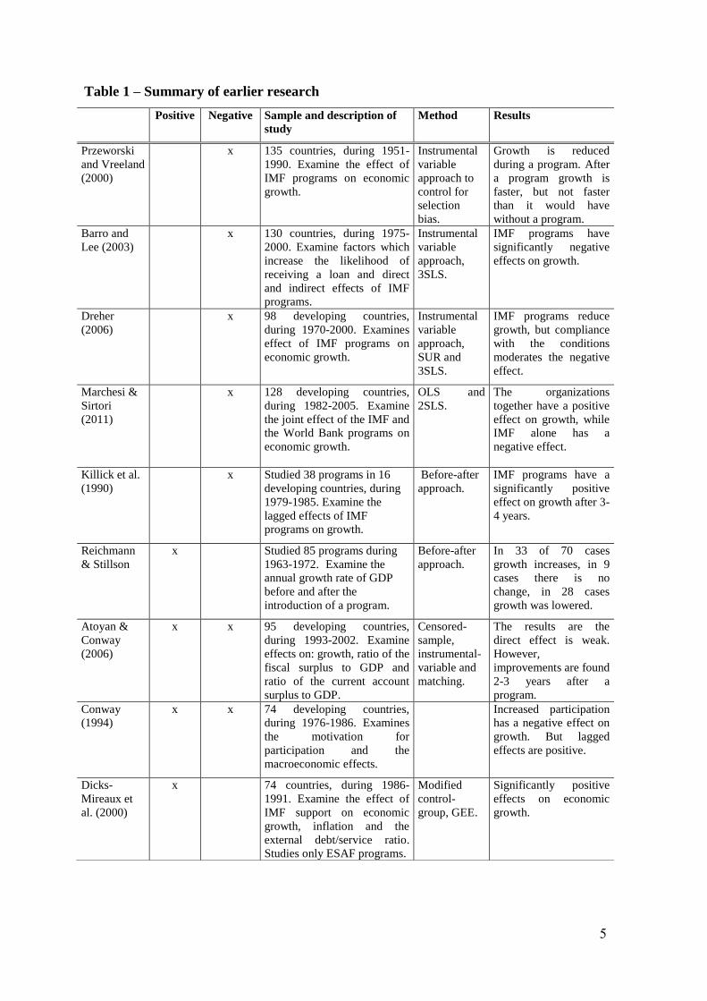
A range of research examines if, and how, the IMF can promote growth. A

summarised selection of these is presented in Table 1, containing descriptions of the

studies, their methods and results. As can be seen the effect is not straightforward.

1 Balance of payment problems occurs when a country no longer is able to meet international payment

obligations (IMF 2008).

5

Table 1 – Summary of earlier research

Positive Negative Sample and description of

study

Method Results

Przeworski

and Vreeland

(2000)

x 135 countries, during 1951-

1990. Examine the effect of

IMF programs on economic

growth.

Instrumental

variable

approach to

control for

selection

bias.

Growth is reduced

during a program. After

a program growth is

faster, but not faster

than it would have

without a program.

Barro and

Lee (2003)

x 130 countries, during 1975-

2000. Examine factors which

increase the likelihood of

receiving a loan and direct

and indirect effects of IMF

programs.

Instrumental

variable

approach,

3SLS.

IMF programs have

significantly negative

effects on growth.

Dreher

(2006)

x 98 developing countries,

during 1970-2000. Examines

effect of IMF programs on

economic growth.

Instrumental

variable

approach,

SUR and

3SLS.

IMF programs reduce

growth, but compliance

with the conditions

moderates the negative

effect.

Marchesi &

Sirtori

(2011)

x 128 developing countries,

during 1982-2005. Examine

the joint effect of the IMF and

the World Bank programs on

economic growth.

OLS and

2SLS.

The organizations

together have a positive

effect on growth, while

IMF alone has a

negative effect.

Killick et al.

(1990)

x Studied 38 programs in 16

developing countries, during

1979-1985. Examine the

lagged effects of IMF

programs on growth.

Before-after

approach.

IMF programs have a

significantly positive

effect on growth after 3-

4 years.

Reichmann

& Stillson

x Studied 85 programs during

1963-1972. Examine the

annual growth rate of GDP

before and after the

introduction of a program.

Before-after

approach.

In 33 of 70 cases

growth increases, in 9

cases there is no

change, in 28 cases

growth was lowered.

Atoyan &

Conway

(2006)

x x 95 developing countries,

during 1993-2002. Examine

effects on: growth, ratio of the

fiscal surplus to GDP and

ratio of the current account

surplus to GDP.

Censored-

sample,

instrumental-

variable and

matching.

The results are the

direct effect is weak.

However,

improvements are found

2-3 years after a

program.

Conway

(1994)

x x 74 developing countries,

during 1976-1986. Examines

the motivation for

participation and the

macroeconomic effects.

Increased participation

has a negative effect on

growth. But lagged

effects are positive.

Dicks-

Mireaux et

al. (2000)

x 74 countries, during 1986-

1991. Examine the effect of

IMF support on economic

growth, inflation and the

external debt/service ratio.

Studies only ESAF programs.

Modified

control-

group, GEE.

Significantly positive

effects on economic

growth.

6

Much research finds a negative effect from the IMF programs on growth (see e.g.

Prezworski & Vreeland 2000, Dreher 2006, Marchesi & Sirtori 2010, Barro & Lee 2003).

Prezworski & Vreeland (2000) conclude that the stabilising effect obtained from the

provision of money is not enough to accelerate growth. Dreher (2006) highlights the low

rates of compliance with policy conditions as an explanation for the negative results.

Marchesi & Sirtori (2010) argue in the same vein. They also withhold that the IMF focuses

on fiscal and monetary discipline, which is argued not fitting the structurally characterised

problems that the poorest countries are likely to face. On the other hand, Barro & Lee

(2003) argue that growth is directly lowered by negative effects induced on investments

and indirectly through lowered rate of openness and rule of law.

Reviewing the progress of the IMF programs in different regions of the world,

mainly negative results are found (see e.g. Stone 2004 on Africa, Ozturk 2008 on South

America, Nunnenkamp 1998, Brouwer 2004 on Asia). These negative results are explained

by the poor preconditions in the regions and a lack of general support for the programs and

the policy conditions. Nevertheless, there are exceptions showing that the IMF programs in

general have positive effects on economic growth (see e.g. Dicks-Mireaux et al. 2000,

Reichmann & Stillson 1987). While some found a lagged positive effect on growth (see

e.g. Killick et al. 1992, Conway 1994, Atoyan & Conway 2006).

Based on earlier findings a relationship between the IMF and economic growth is

assumed. The dispersion of earlier research on the effects on growth encourages us to

examine in which way they are connected. Starting with an examination of the overall

effect of IMF programs on economic growth, our aim is to determine whether the effect is

positive or negative. To widen this examination a set of dummy variables is used in three

additional models. The second model estimates differences between three decades: 1980,

1990, and 2000. The third model estimates difference between programs: SBA, ECF, EFF,

SAF, ESF and FCL. Finally, the fourth model estimates difference between regions:

Africa, Asia and South America. One type of growth strategy is to initiate economic

growth with a short-term kick start of the economy, followed by long-term reforms to

sustain growth (Rodrik 2003). In spirit of this theory the thesis is aimed at estimating the

short-term2 effect on growth.

The examination is based on a panel consisting of observations from 86 developing

countries during 1983-2010. The methods of assessment are ordinary least squares (OLS)

2 Our models consist of three equations, testing the effect on growth without any lags, with a one-year lag

and with a two-year lag. Thus, the short-term effect is defined as zero up to two years.

7

and two-stage least squares (2SLS). In the sample, 11.63% of the countries have never

received a loan disbursement from the IMF. The remaining 88.37%, consisting of 76

countries, have received loan disbursements from at least one of the six different types of

programs3. In earlier research the main focus has been to answer if the IMF has a

significant effect growth. Yet, no research has been found that controls for the effects on

growth of the different kinds of programs, nor during the 1980s, 1990s or 2000s. This

thesis contributes with an examination in these areas. Earlier research has mainly included

the two most common programs: the Stand-by arrangements (SBA) and Extended fund

facility (EFF) (see e.g. Barro & Lee 2003, Dreher 2006). But some researchers have

compared these two programs with the Structural adjustment fund (SAF) and Extended

structural adjustment fund (ESAF) (see e.g. Evrensel 2002, Evrensel & Kim 2006).

The following section provides basic information on the IMF and six different kinds

of programs. Section three provides descriptive evidence of our data. Section four provides

a theoretical approach on how the IMF can affect growth, our growth model and the

regression results. The results are presented with a discussion on possible explanations.

The final section provides a summary and some concluding remarks.

3 This study covers Stand-by arrangements (SBA), Extended fund facility (EFF), Flexible credit line (FCL),

Structural adjustment facility (SAF), Exogenous shock facility (ESF) and the Extended credit facility (ECF).

8

2. Definitions

2.1 The IMF

The IMF is an international organization working for economic cooperation and stability.

It currently consists of 188 member countries (IMF 2013f). The organization was created

in 1944 as one of the foundations of the Bretton Woods system4. The initial purpose of the

organization was to guarantee the fixed exchange rates and to deal with temporary deficits

through financial support (Barro & Lee 2003, IMF 2013b). The mandate of the IMF

changed as the fixed gold standard was dropped. The IMF’s work expanded towards new

areas (Bauer et al. 2009).

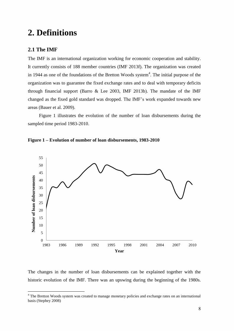
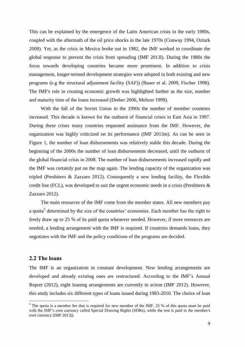
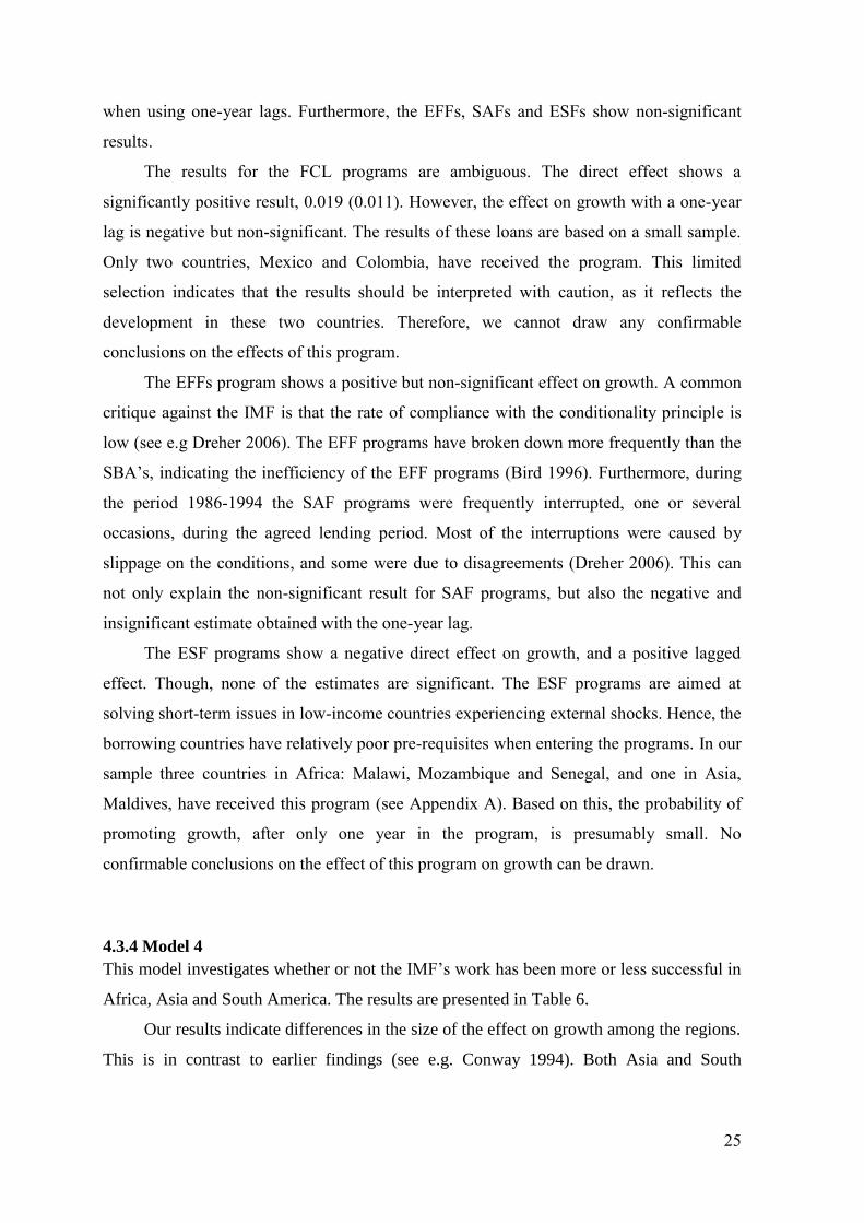
Figure 1 illustrates the evolution of the number of loan disbursements during the

sampled time period 1983-2010.

Figure 1 – Evolution of number of loan disbursements, 1983-2010

The changes in the number of loan disbursements can be explained together with the

historic evolution of the IMF. There was an upswing during the beginning of the 1980s.

4 The Bretton Woods system was created to manage monetary policies and exchange rates on an international

basis (Stephey 2008)

0

5

10

15

20

25

30

35

40

45

50

55

1983 1986 1989 1992 1995 1998 2001 2004 2007 2010

Nu

mb

er o

f lo

an

dis

bu

rsem

ents

Year

9

This can be explained by the emergence of the Latin American crisis in the early 1980s,

coupled with the aftermath of the oil price shocks in the late 1970s (Conway 1994, Ozturk

2008). Yet, as the crisis in Mexico broke out in 1982, the IMF worked to coordinate the

global response to prevent the crisis from spreading (IMF 2013l). During the 1980s the

focus towards developing countries became more prominent. In addition to crisis

management, longer-termed development strategies were adopted in both existing and new

programs (e.g the structural adjustment facility (SAF)) (Bauer et al. 2009, Fischer 1998).

The IMF's role in creating economic growth was highlighted further as the size, number

and maturity time of the loans increased (Dreher 2006, Meltzer 1999).

With the fall of the Soviet Union in the 1990s the number of member countries

increased. This decade is known for the outburst of financial crises in East Asia in 1997.

During these crises many countries requested assistance from the IMF. However, the

organization was highly criticized on its performance (IMF 2013m). As can be seen in

Figure 1, the number of loan disbursements was relatively stable this decade. During the

beginning of the 2000s the number of loan disbursements decreased, until the outburst of

the global financial crisis in 2008. The number of loan disbursements increased rapidly and

the IMF was certainly put on the map again. The lending capacity of the organization was

tripled (Presbitero & Zazzaro 2012). Consequently a new lending facility, the Flexible

credit line (FCL), was developed to suit the urgent economic needs in a crisis (Presbitero &

Zazzaro 2012).

The main resources of the IMF come from the member states. All new members pay

a quota5 determined by the size of the countries’ economies. Each member has the right to

freely draw up to 25 % of its paid quota whenever needed. However, if more resources are

needed, a lending arrangement with the IMF is required. If countries demands loans, they

negotiates with the IMF and the policy conditions of the programs are decided.

2.2 The loans

The IMF is an organization in constant development. New lending arrangements are

developed and already existing ones are restructured. According to the IMF’s Annual

Report (2012), eight loaning arrangements are currently in action (IMF 2012). However,

this study includes six different types of loans issued during 1983-2010. The choice of loan

5 The quota is a member fee that is required for new member of the IMF. 25 % of this quota must be paid

with the IMF’s own currency called Special Drawing Rights (SDRs), while the rest is paid in the member's

own currency (IMF 2013j).

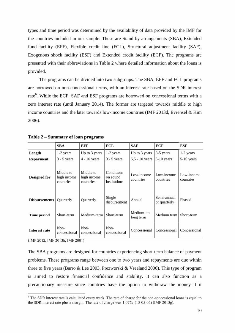
10

types and time period was determined by the availability of data provided by the IMF for

the countries included in our sample. These are Stand-by arrangements (SBA), Extended

fund facility (EFF), Flexible credit line (FCL), Structural adjustment facility (SAF),

Exogenous shock facility (ESF) and Extended credit facility (ECF). The programs are

presented with their abbreviations in Table 2 where detailed information about the loans is

provided.

The programs can be divided into two subgroups. The SBA, EFF and FCL programs

are borrowed on non-concessional terms, with an interest rate based on the SDR interest

rate6. While the ECF, SAF and ESF programs are borrowed on concessional terms with a

zero interest rate (until January 2014). The former are targeted towards middle to high

income countries and the later towards low-income countries (IMF 2013d, Evrensel & Kim

2006).

Table 2 – Summary of loan programs

SBA EFF FCL SAF ECF ESF

Length 1-2 years Up to 3 years 1-2 years Up to 3 years 3-5 years 1-2 years

Repayment 3 - 5 years 4 - 10 years 3 - 5 years 5,5 - 10 years 5-10 years 5-10 years

Designed for

Middle to

high income

countries

Middle to

high income

countries

Conditions

on sound

institutions

Low-income

countries

Low-income

countries

Low-income

countries

Disbursements Quarterly Quarterly Single

disbursement Annual

Semi-annual

or quarterly Phased

Time period Short-term Medium-term Short-term Medium- to

long term Medium term Short-term

Interest rate Non-

concessional

Non-

concessional

Non-

concessional Concessional Concessional Concessional

(IMF 2012, IMF 2013h, IMF 2001)

The SBA programs are designed for countries experiencing short-term balance of payment

problems. These programs range between one to two years and repayments are due within

three to five years (Barro & Lee 2003, Prezworski & Vreeland 2000). This type of program

is aimed to restore financial confidence and stability. It can also function as a

precautionary measure since countries have the option to withdraw the money if it

6 The SDR interest rate is calculated every week. The rate of charge for the non-concessional loans is equal to

the SDR interest rate plus a margin. The rate of charge was 1.07% (13-05-05) (IMF 2013g).

11

becomes necessary. The purpose of these programs is to signal to investors that

improvements in the economic environment are to come (Fischer 1997).

The EFF programs are designed for countries experiencing long-termed balance of

payments problems. It is also aimed at supporting major structural reforms. This structural

agenda is reflected in the conditions attached to the programs. The programs last up to four

years with repayments due after four to ten years (IMF 2012).

The FCL programs are designed for countries experiencing all types of balance of

payments problems. As with the SBAs, it can either be aimed at solving already existing

issues, or to serve as a precautionary measure. However, the program is new in its design

since it has a prequalification criterion instead of the conditionality principle. The countries

qualifying for these loans must have strong institutions since they are trusted to implement

the correct policies to restore balance (John and Knedlik 2011). The programs are issued in

one disbursement with repayment between three to five years (IMF 2013d).

The SAF programs are some of the first targeted towards low-income countries. The

SAF programs are the only lending arrangement in our sample that is no longer in use7.

These programs could last up to three years, with repayment between five to ten years

(IMF 2001). The loans were borrowed on concessional terms and resembled foreign aid

(Barro & Lee 2003, IMF 2004).

The ECF programs are targeted towards low-income countries. These programs are

designed for countries experiencing prolonged balance of payments problems. The

programs last three to five years and repayments are due within five to ten years (IMF

2013d, IMF 2013h). As with the EFF programs, the conditions attached are focused on

structural policy reforms. However, in addition these programs include poverty reduction

policies (IMF 2012).

The ESF is a new type of program designed for low-income countries facing urgent

balance of payments problems caused by external shocks (IMF 2013d). These programs

range between one to two years and repayments are due within five to ten years (IMF

2013k).

7 These programs were active during 1986-1995 (IMF 2004).

12

3. Descriptive Evidence

This section provides descriptive evidence of our data set. The data for the control

variables is collected from the databases: Penn World Tables, Barro & Lee and the World

Bank. The original resources are presented in Appendix C. Data on the loan disbursements

are collected using IMFs own records, displayed on their webpage (see Appendix A). The

panel includes 86 countries, during 1983-2010 and is balanced.

To get an understanding of the data, Appendix A presents a table with all the

countries included. It also specifies which region the countries belong to, what kind of

programs they have received and during what years the programs were in action. Our

analysis is based on this information. Restricting the examination to only include

developing countries contributes to a homogeneous dataset. It also facilitates the analysis,

as countries with similar income levels tend to grow in a similar manner (Jones 2002, p.

127-132). The countries included in our analysis are ranging from low to upper-middle

income economies (i.e. 1.025 dollar or less to a maximum of 12.475 dollars a day) (World

Bank 2013a).

Cross-section data often suffers from problems of heteroskedasticity, while time-

series data often have problems with non-stationarity and autocorrelation (Verbeek 2008,

p. 88-89, 104-105, 270-271). Therefore non-stationarity, heteroskedasticity and

autocorrelation are controlled for and detailed information on the tests performed can be

found in Appendix B. These problems are corrected for by logging and differentiating the

series and using White’s standard errors (diagonal) in all the regressions.

The data on loan disbursements show which countries that have received financial

support from the IMF. A total number of 166 loan disbursements have been issued during

1983-2010. Most commonly one program is active at the time though there are examples

of countries being in multiple arrangements (e.g. Burundi that had both a SBA and SAF

program during 1986-1988, see Appendix A). The distribution of loan types in our sample

show that SBAs have been granted to 80.23% of the countries, ECFs to 45.35%, EFFs to

29.10%, SAFs to 31.40%, ESFs to 4.65% and FCLs to 2.33% (see Appendix A).

The programs are active during different time periods. In our data the SBAs and

EFFs are active the entire time period. The SAF programs are active only during the 1980s

and 1990s. Both the ESF and FCL programs are rather new arrangements and have only

been active since the 2000s. (See Appendix A).

13

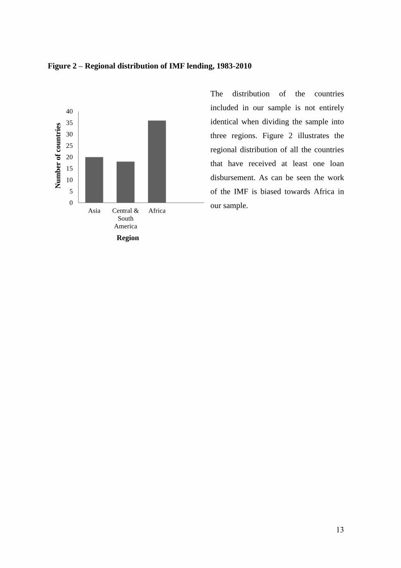
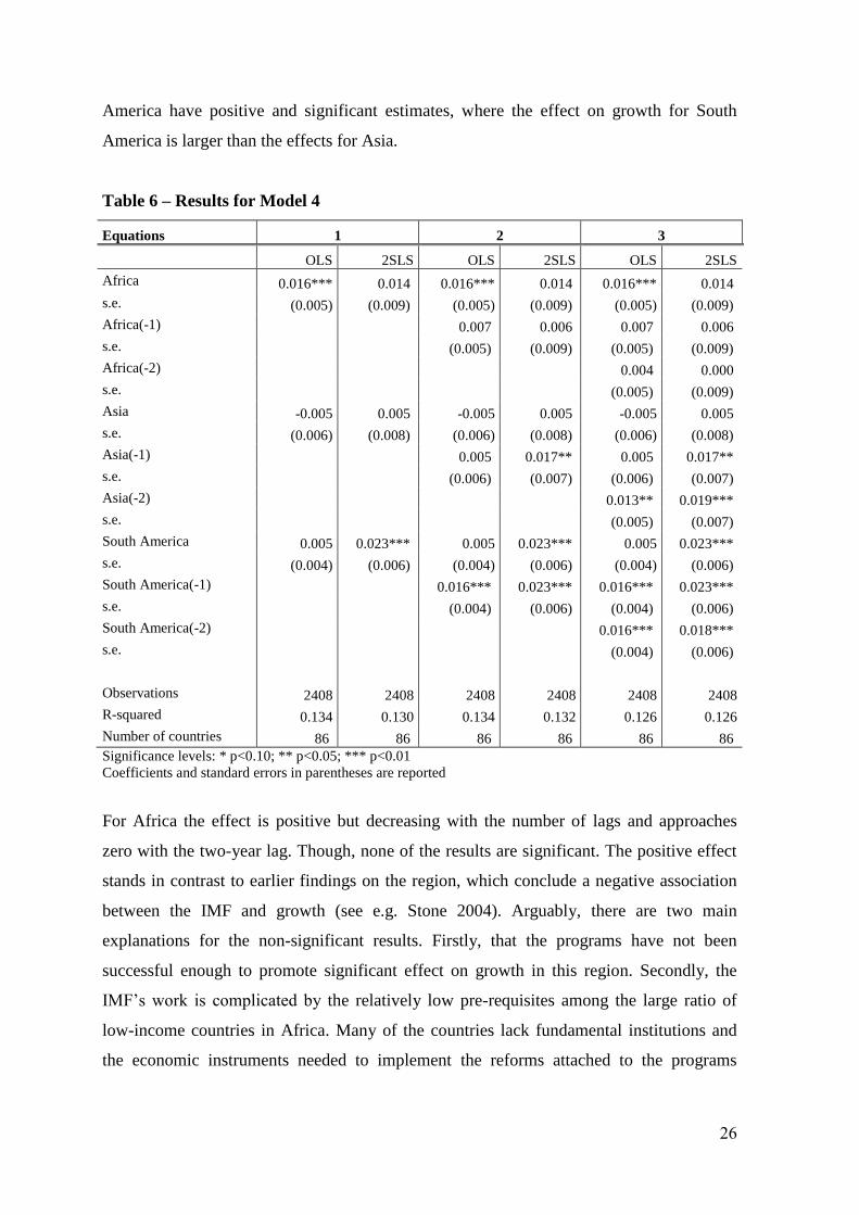
Figure 2 – Regional distribution of IMF lending, 1983-2010

The distribution of the countries

included in our sample is not entirely

identical when dividing the sample into

three regions. Figure 2 illustrates the

regional distribution of all the countries

that have received at least one loan

disbursement. As can be seen the work

of the IMF is biased towards Africa in

our sample.

0

5

10

15

20

25

30

35

40

Asia Central &

South

America

Africa

Nu

mb

er o

f co

un

trie

s

Region

14

4. The IMF and economic growth

4.1. Theoretical channels of impact

A wide amount of theoretical literature highlights several channels through which the IMF

influences economic growth in either a positive or negative way. In sprit of Dreher (2006)

four main channels of impact are presented. Both positive and negative aspects are

highlighted to get a full image of the IMF’s ability to promote growth.

The first channel focuses on the provision of money, including the creation of credit

and liquidity. This channel can be viewed as an immediate, short-term solution aimed at

stabilising the economic development. Thereby, it creates the necessary conditions for

sustained economic growth (Fischer 1997). On the other hand, there is a risk that the effect

is diffused. The provision of money can create disincentives to reform the economy, which

can result in governments keeping inappropriate policies. Such moral hazards can appear if

the performance criteria are not enforced, i.e. the actual costs of entering a program are

lower than the expected (Dreher 2006, Stone 2004).

Furthermore, the existence of the IMF, acting as a lender of last resort, can create

another type of moral hazard. This can create incentives for countries to adopt infeasible

economic policies long before any loan arrangement is required (Evrensel & Kim 2006,

Dreher 2006). Thus, if sound policies are not adopted the issue of moral hazards can lead

to the creation of a dependency on the IMF (Stone 2004).

Second, the programs also serve as insurance. By setting its “seal of approval” the

IMF enhances the credibility of the countries’ financial policies and development. The

programs ensure, and can even attract more investors (Bauer et. al 2009, Bird & Rowlands

2001). The programs can have an essential function to enable countries to acquire other

public and private loans as well (Fischer 1997). On the other hand, participating in an IMF

program can be viewed as a sign of economic distress. This indicates that the “seal of

approval” set by the IMF does not carry enough market value to affect investors’

expectations (Bird 1996, Bauer et. al 2009).

Third, the conditions attached to the programs reassure the commitment to a

particular set of macroeconomic policies. However, increasing economic growth is not

included under the programs conditionality principles. Growth is instead set as an

indicative target and a desired outcome of the actual performance criteria (Fischer 1997,

Evrensel 2002). The conditions can include both fiscal austerity and tighter monetary

15

policies through measures such as: cutting government expenditures, increasing taxes,

raising interest rates and devaluing currencies (Abbott et al 2009, Prezworski & Vreeland

2000).

As the focus of the IMF’s work changed, it more commonly promoted structural

policies. Typical reforms were changing the patterns of government spending, restructuring

banking systems as well as liberalizing prices and trade (Bird 1996, Fischer 1997).

However, the effectiveness of the programs to affect growth is dependent on the rate of

compliance with the policy conditions (Jorra 2011). The rate of compliance differs across

countries, indicating that it dependent on the prerequisites of the borrowing countries, such

as their institutions and type of regime. For instance, democracies with reliable institutions

are found to have a tendency to do better than other types of regimes (Bauer et al. 2009).

Fourth, the IMF can influence growth by providing information through surveillance

and financial advice to its member countries. This is done by monitoring the international

monetary system and changes in economic policies. Through forecasts, instabilities can be

detected and measures to prevent their outbursts can be taken (IMF 2013b).

4.2 The growth model

In spirit of Neo-classical theory, the model applied in this study is based on the classical

Solow growth model with technology, where a Cobb-Douglas production function is

assumed: . The model is built on three main factors of influence: stock of

capital (K), labour (L), and technology (A). The technological progress is assumed to be

exogenous in the model. (Jones 2002, p. 36) However, it will be considered in more

general terms as the total factor productivity (TFP) in our model.

The TFP is aimed at capturing the efficiency of a country’s inputs, including both

physical and human capital (Jones 2002, p. 146-147). Thus, the effects of the four

theoretical channels are captured by the TFP, represented by A in the production function.

The channels are assumed to enhance a productive use of resources and to encourage

reforms on policies currently preventing a country from developing.

To capture the effect of these channels, a set of dummy variables is used. To make

this study possible the analysis is divided into four models. All the models have the

purpose to examine if the IMF promotes growth. Model 1 tests the general effect on

growth when given an additional annual loan disbursement. Model 2 tests the specific

effects for three decades. This is done by including dummy variables for 1980, 1990 and

16

2000. Model 3 tests the effects of different kinds of loans, including dummy variables for

the six different lending arrangements: SBA, ECF, EFF, SAF, ESF and FCL. Model 4 tests

the effects of three regions, including dummy variables for Africa, Asia and South

America. The dummy variables take the value one for each year a country receives a loan

disbursement, and zero for all other years.

To be able to examine the effects of the dummy variables on growth, control

variables are needed. The control variables chosen are based on earlier research (see e.g.

Barro & Sala-i-Martin 2004, p. 521-533). The variables represent a country’s physical and

human capital stock, general health and infrastructure. In all the regression models the

following control variables will be used: the stock of capital ( ), average total years of

schooling ( )8, fertility rate ( , rate of openness ( )

9 and life expectancy at

birth ( ). In accordance with Barro & Sala-i-Martin (2004) the stock of real capital,

education, openness and life expectancy are expected to have a positive effect on economic

growth, while fertility rate is expected to have a negative effect.

To enable the use of a linear regression model, the production function is

transformed. The descriptive alternations of all the variables and sources can be seen in

detail in Appendix C. While the descriptive data on all the variables can be found in

Appendix D. The general model tested is:

( ( ( ( ( ( (

where represents GDP per capita growth in country i at period t. represents the

groups of dummy variables tested in each of the four models (the specific regression

models can be seen in Appendix F). Since the countries in our sample cannot be

considered randomly chosen, fixed effects are used. Therefore, a fixed effects two way

error component model is applied. The two way error component includes: a time

independent country fixed effect ( ,) which allows the countries to have an individual

intercept; a time dependent fixed effect ( ), which allows time dependent effects that are

common to all the countries; the ordinary disturbance term ( , which varies with

countries and time.

8 Human capital is often explained in growth models as time spent on education; see e.g. the Solow model

with human capital and the Lucas model (1988) in Jones 2002, p. 55, 161 9 Openness is measured as export minus import divided by GDP (University of Pennsylvania 2008).

17

The regression analysis is conducted using both OLS and 2SLS estimations. The

methods differ on the requirements of the explanatory variables. The OLS yields reliable

results with exogenous explanatory variables. This means that they are determined outside

the model and that they are not correlated with the error term (Hill et al. 2008, p. 276).

However, there is a risk that the dummy variables are not exogenous since the IMF

programs often are concluded in periods of economic crisis. This means that the dummy

variables affect growth, while at the same time growth affects the dummy variables. If this

is the case the dummy variables reflect the negative effects of the underlying crisis (Dreher

2006).

The 2SLS, on the other hand, can account for endogenous explanatory variables. By

including instrumental variables the effects of the dummy variables on growth is isolated

and the estimates yield consistent results. An instrumental variable should be correlated

with the endogenous variable but not with the error term. In addition, it should not have a

direct effect on the explained variable (Hills et al. 2008, p. 278). In our growth model

internal instruments are used, represented by lagged dummy variables. The choice of

instruments is motivated by the high probability that the dummy variables are correlated

with its own lags. However, it is unlikely that the need for a loan is based on information

on future growth. Rather the decision is based on the issues seen today. Hence, the dummy

variables do not have a direct effect on the explained variable.

4.3 Regression results

The regression results are divided into four sections representing each model. Since the

focus of this thesis is to examine the effects on growth from programs, the results of the

dummy variables is at focus. The estimates for the dummy variables alone are shown in

Table 3-6 and each table represents one model. However the full results, including both

control variables and dummy variables, can be seen in Appendix E.

Three columns are presented in each table, representing the different equations

estimated in each model. The first equation examines the direct effect on growth, the

second equation the one-year lagged effect and the third equation the two-year lagged

effect. This means that the effect of the loan disbursements on growth is seen with one

respectively two year’s hindsight. The lagged estimates test the sensitivity of the results. If

the estimates are consistent among the lags the results are considered to be robust. The left

part of each column shows the OLS estimates and the right part the 2SLS estimates. The

18

main focus of the analysis is the results of the 2SLS estimates since they account for

endogeneity.

Even though the focus is on the dummy variables, some concluding remarks must be

made on the control variables. The results are in general inconclusive. The stock of capital,

education, fertility rate and life expectancy all have positive effects on growth. However

the results are not robust, since the lagged estimates change signs and are non-significant.

As described in Appendix C, the stock of capital was calculated and education

interpolated. The stock of capital, education and life expectancy have high standard errors

and show inconclusive results. The positive estimates for fertility rate stands in contrast to

earlier research (see e.g. Barro & Sala-i-Martin 2004, p. 525). Only openness has a

negative effect on growth. However, when lagging one year the effect is positive and

significant.

The estimated coefficient of the intercept is approximately 0.012, representing an

averaged intercept for the countries in the panel. Since not all countries in our sample have

received loans there is no reference dummy and the intercept is included. This means that

the estimates for the dummy variables are interpreted as an additional effect on growth. All

regression equations show low R-square values. The low rates of explanation can be due to

high variance in the data which is common for developing countries. Bird & Rowlands

(2001) points out that a feature among some earlier research on the IMF and growth, is a

poor overall explanatory power. This problem is explained to be caused by omitted

variables. A growth model can include many explanatory factors, and it is impossible to

capture them all.

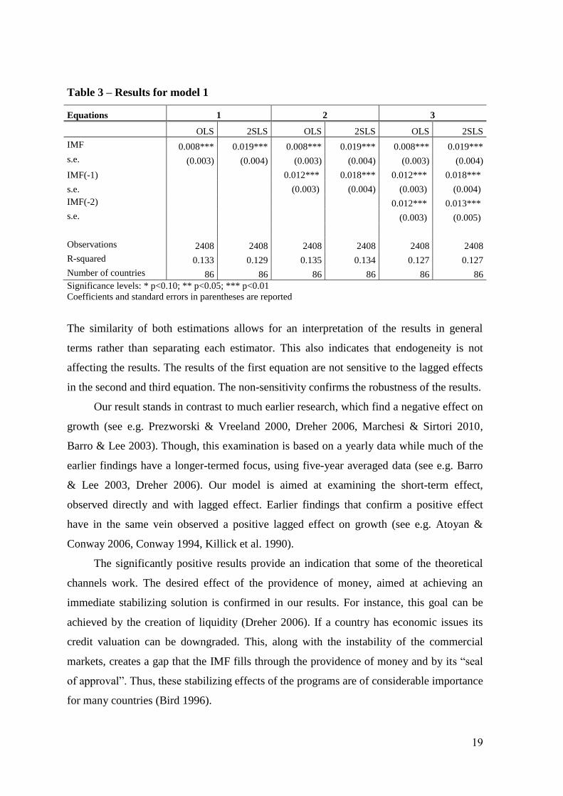
4.3.1 Model 1

This model tests the overall effect of the annual loan disbursements on economic growth.

The results are presented in Table 3.

All estimates show that the loan disbursements have a positive and significant effect

on economic growth at the one percentage level. The largest effect on growth is obtained

by the 2SLS estimate of the first equation. The coefficient, 0.019 (0.004), indicates that the

effect of an annual loan disbursement raises growth with 1.9 % during the same year. The

2SLS estimates show that the positive effect on growth is slowly decreasing with the

number of lags. While the positive effect of the OLS estimates is slowly increasing with

the number of lags.

19

Table 3 – Results for model 1

Equations 1 2 3

OLS 2SLS OLS 2SLS OLS 2SLS

IMF 0.008*** 0.019*** 0.008*** 0.019*** 0.008*** 0.019***

s.e. (0.003) (0.004) (0.003) (0.004) (0.003) (0.004)

IMF(-1) 0.012*** 0.018*** 0.012*** 0.018***

s.e. (0.003) (0.004) (0.003) (0.004)

IMF(-2) 0.012*** 0.013***

s.e. (0.003) (0.005)

Observations 2408 2408 2408 2408 2408 2408

R-squared 0.133 0.129 0.135 0.134 0.127 0.127

Number of countries 86 86 86 86 86 86

Significance levels: * p<0.10; ** p<0.05; *** p<0.01

Coefficients and standard errors in parentheses are reported

The similarity of both estimations allows for an interpretation of the results in general

terms rather than separating each estimator. This also indicates that endogeneity is not

affecting the results. The results of the first equation are not sensitive to the lagged effects

in the second and third equation. The non-sensitivity confirms the robustness of the results.

Our result stands in contrast to much earlier research, which find a negative effect on

growth (see e.g. Prezworski & Vreeland 2000, Dreher 2006, Marchesi & Sirtori 2010,

Barro & Lee 2003). Though, this examination is based on a yearly data while much of the

earlier findings have a longer-termed focus, using five-year averaged data (see e.g. Barro

& Lee 2003, Dreher 2006). Our model is aimed at examining the short-term effect,

observed directly and with lagged effect. Earlier findings that confirm a positive effect

have in the same vein observed a positive lagged effect on growth (see e.g. Atoyan &

Conway 2006, Conway 1994, Killick et al. 1990).

The significantly positive results provide an indication that some of the theoretical

channels work. The desired effect of the providence of money, aimed at achieving an

immediate stabilizing solution is confirmed in our results. For instance, this goal can be

achieved by the creation of liquidity (Dreher 2006). If a country has economic issues its

credit valuation can be downgraded. This, along with the instability of the commercial

markets, creates a gap that the IMF fills through the providence of money and by its “seal

of approval”. Thus, these stabilizing effects of the programs are of considerable importance

for many countries (Bird 1996).

20

Decreasing creditworthiness is a key factor driving the demand for IMF loans and the

severity of the problems increases the persistency of the demand (Bird 1996). Instability

discourages investments and lowers growth (IMF 2013e). In addition, countries with poor

prerequisites, in terms of low rates of investments and slow growth, need support from the

IMF (Bird 1996). These countries need money, certification or precautionary loan

agreements to attract and send signal to investors, raising their expectations (Bird &

Rowlands 2001, Fischer 1997). Our results indicate positive effect of the “seal-of-

approval”, set by participation in programs, since it signals to markets and investors that

the economic issues are to be overcome.

The positive results cannot neither confirm nor reject the existence of moral hazards.

Either it can be an indication that moral hazards are not common in our sampled countries,

or it can be a pure reflection of the providence of money easing acute issues. This enables

countries to keep unwise policies longer, in order to qualify for more IMF programs further

ahead (Meltzer 1999, Evrensel 2002).

In the same sense, no confirmable conclusions can be drawn regarding the rate of

compliance with policies attached to the programs. A high compliance rate is assumed to

increases the effectiveness of the programs. Though, the positive effects in our results

slowly decrease with the number of lags. This might be an indication that the rate of

compliance is low and the policies necessary to uphold sustained growth are not

implemented. Hence, explaining the decline in the size of the positive effect.

4.3.2 Model 2

This model examines the impact of the loan disbursements by controlling for each decade

in our sample. This model investigates whether or not the IMF’s work has been more or

less successful throughout time. The results are presented in Table 4.

In accordance with Model 1, both the OLS and 2SLS estimates shows similar results

and nearly all the estimates are positive. Most of the 2SLS estimates are of greater size.

These estimates also yield significant results in more cases. Furthermore, the negative

result for the 2SLS estimate for the 1990s indicates that endogeneity is affecting the

results. Though, none of the estimates yield significant results for the 1990s. Therefore, we

can conclude that the IMF’s work was successful in raising economic growth during the

1980s and 2000s.

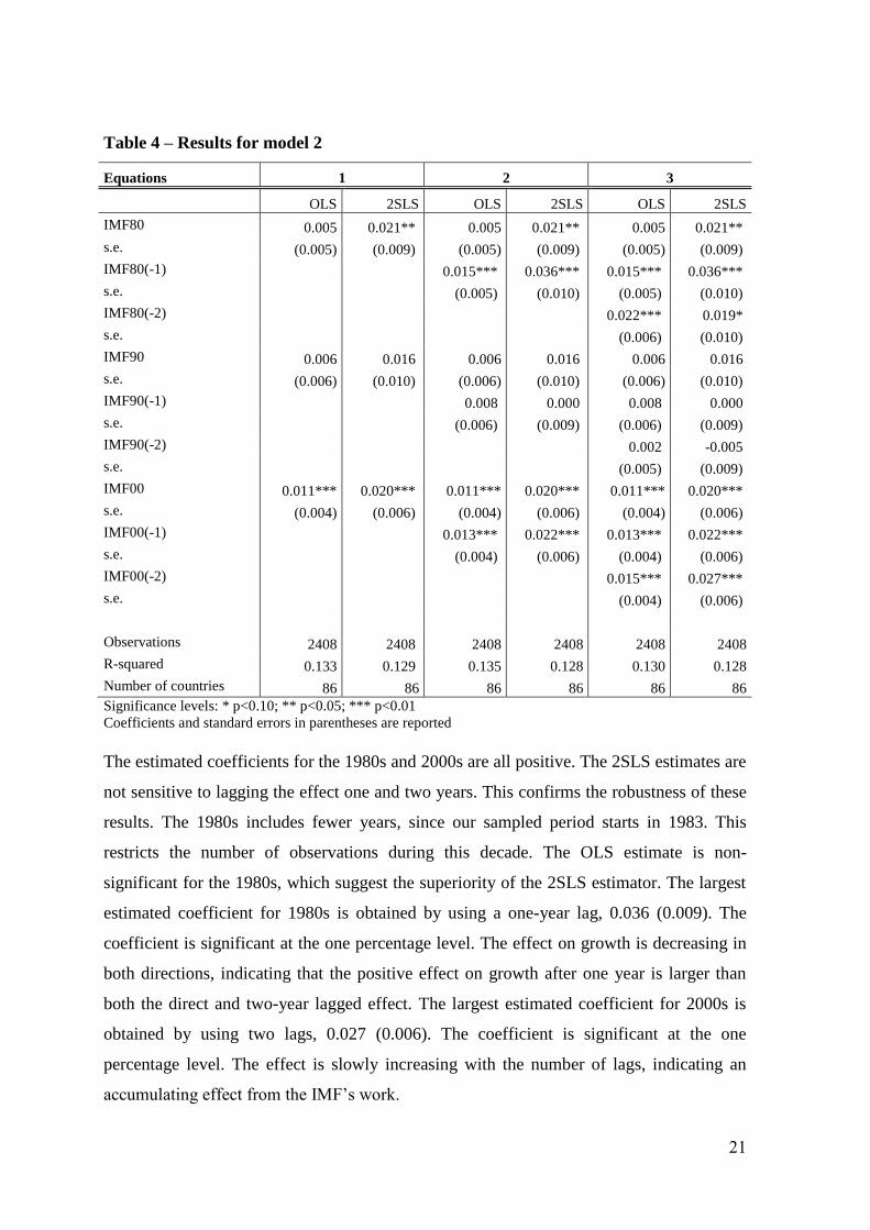
21

Table 4 – Results for model 2

Equations 1 2 3

OLS 2SLS OLS 2SLS OLS 2SLS

IMF80 0.005 0.021** 0.005 0.021** 0.005 0.021**

s.e. (0.005) (0.009) (0.005) (0.009) (0.005) (0.009)

IMF80(-1) 0.015*** 0.036*** 0.015*** 0.036***

s.e. (0.005) (0.010) (0.005) (0.010)

IMF80(-2) 0.022*** 0.019*

s.e. (0.006) (0.010)

IMF90 0.006 0.016 0.006 0.016 0.006 0.016

s.e. (0.006) (0.010) (0.006) (0.010) (0.006) (0.010)

IMF90(-1) 0.008 0.000 0.008 0.000

s.e. (0.006) (0.009) (0.006) (0.009)

IMF90(-2) 0.002 -0.005

s.e. (0.005) (0.009)

IMF00 0.011*** 0.020*** 0.011*** 0.020*** 0.011*** 0.020***

s.e. (0.004) (0.006) (0.004) (0.006) (0.004) (0.006)

IMF00(-1) 0.013*** 0.022*** 0.013*** 0.022***

s.e. (0.004) (0.006) (0.004) (0.006)

IMF00(-2) 0.015*** 0.027***

s.e. (0.004) (0.006)

Observations 2408 2408 2408 2408 2408 2408

R-squared 0.133 0.129 0.135 0.128 0.130 0.128

Number of countries 86 86 86 86 86 86

Significance levels: * p<0.10; ** p<0.05; *** p<0.01

Coefficients and standard errors in parentheses are reported

The estimated coefficients for the 1980s and 2000s are all positive. The 2SLS estimates are

not sensitive to lagging the effect one and two years. This confirms the robustness of these

results. The 1980s includes fewer years, since our sampled period starts in 1983. This

restricts the number of observations during this decade. The OLS estimate is non-

significant for the 1980s, which suggest the superiority of the 2SLS estimator. The largest

estimated coefficient for 1980s is obtained by using a one-year lag, 0.036 (0.009). The

coefficient is significant at the one percentage level. The effect on growth is decreasing in

both directions, indicating that the positive effect on growth after one year is larger than

both the direct and two-year lagged effect. The largest estimated coefficient for 2000s is

obtained by using two lags, 0.027 (0.006). The coefficient is significant at the one

percentage level. The effect is slowly increasing with the number of lags, indicating an

accumulating effect from the IMF’s work.

22

The 1980s is characterized by a structurally oriented development of IMF programs,

aimed at fostering growth. This development is targeted towards low-income countries

(Easterly 2005). Typically occurring programs during this decade are SBAs and ECFs. A

pattern can be seen for these programs, as they are often given after each other (see

Appendix A). This setup can confirm the structurally based focus of the IMF’s work,

which corresponds to established growth strategy10

. The SBA programs are aimed at

solving short-term issues, while the ECFs are aimed at longer-termed structural reforms.

Our results show a large positive effect on growth with a one-year lag. This result can

serve as an indication that the shorter-termed problems are corrected. The positive effect is

smaller with a two-year lag. Hence the positive effect on growth decreases slowly

suggesting that further assistance is needed, which the combination with ECF programs

provides.

Examining the 1990s none of the estimates are significant. The first equation shows

that the direct effect is positive. The effect is then decreasing with the number of lags and

is negative with a two-year lag. Hence, these results leave no confirmable conclusions for

this decade.

In contrast, a positive effect on growth is shown during the 2000s. Based on the

emergence of the financial crisis in 2008, the explanation of the overall positive results is

twofold. On the one hand, there is usually a boom before the bust. Heading towards the

crisis growth rates flourished contributing to a general positive development. On the other

hand, it can be explained by the development of a consensus on the economic institutions

necessary for stable growth. Some examples are setting inflation targets, higher rate of

surveillance of the financial markets and restricting budget deficits (Borio & White 2004).

These kinds of targets facilitate the IMF’s work, as it creates a general confidence in the

policies attached to the programs. The positive effect shown in our results is increasing

with the number of lags. This accumulating effect of the IMF’s work also indicates a high

efficiency of the attached policies during this decade in promoting growth.

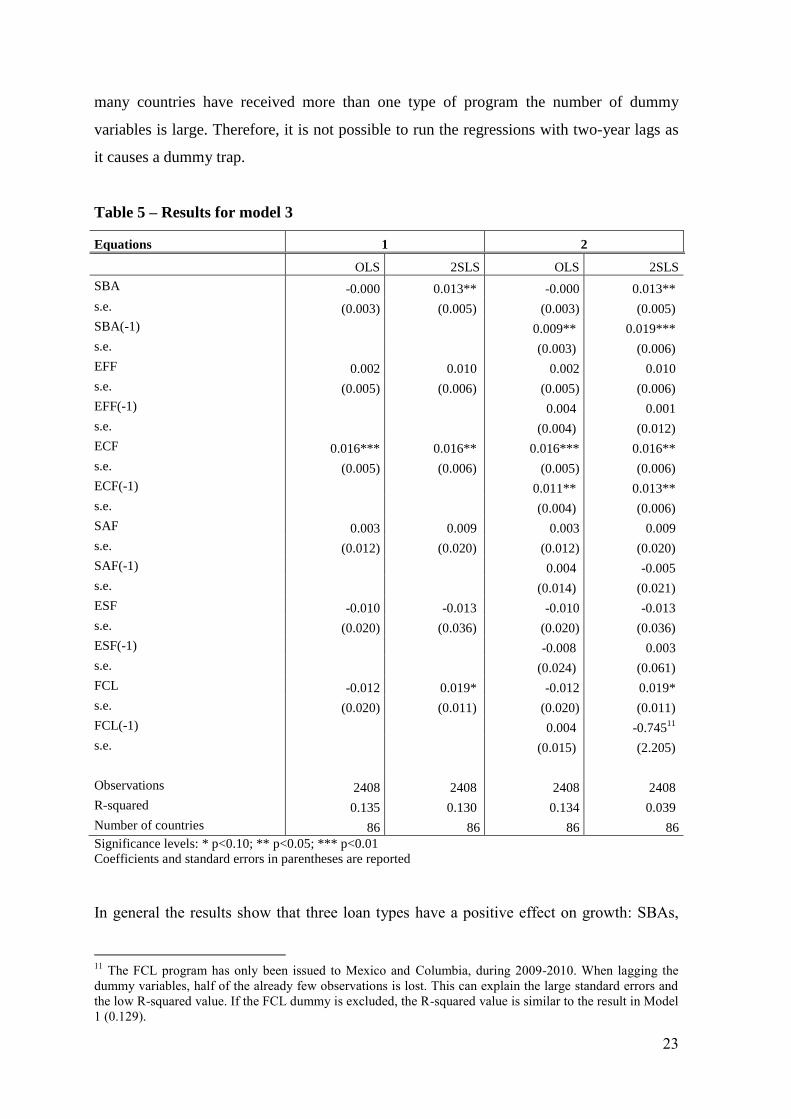
4.3.3 Model 3

This model examines the effect from the different kinds of programs on growth. The

results are presented in Table 5. This model is restricted to using one-year lags. Since

10

In Rodrik (2003) a growth strategy is presented. It emphasizes the enforcement of policies that kick-start

the economy (in the way the SBA’s do by solving short-term problems), while at the same implementing

long-term policies that can sustain the increased economic growth (in the same way as the ECF’s structural

reforms).

23

many countries have received more than one type of program the number of dummy

variables is large. Therefore, it is not possible to run the regressions with two-year lags as

it causes a dummy trap.

Table 5 – Results for model 3

Equations 1 2

OLS 2SLS OLS 2SLS

SBA -0.000 0.013** -0.000 0.013**

s.e. (0.003) (0.005) (0.003) (0.005)

SBA(-1) 0.009** 0.019***

s.e. (0.003) (0.006)

EFF 0.002 0.010 0.002 0.010

s.e. (0.005) (0.006) (0.005) (0.006)

EFF(-1) 0.004 0.001

s.e. (0.004) (0.012)

ECF 0.016*** 0.016** 0.016*** 0.016**

s.e. (0.005) (0.006) (0.005) (0.006)

ECF(-1) 0.011** 0.013**

s.e. (0.004) (0.006)

SAF 0.003 0.009 0.003 0.009

s.e. (0.012) (0.020) (0.012) (0.020)

SAF(-1) 0.004 -0.005

s.e. (0.014) (0.021)

ESF -0.010 -0.013 -0.010 -0.013

s.e. (0.020) (0.036) (0.020) (0.036)

ESF(-1) -0.008 0.003

s.e. (0.024) (0.061)

FCL -0.012 0.019* -0.012 0.019*

s.e. (0.020) (0.011) (0.020) (0.011)

FCL(-1) 0.004 -0.74511

s.e. (0.015) (2.205)

Observations 2408 2408 2408 2408

R-squared 0.135 0.130 0.134 0.039

Number of countries 86 86 86 86

Significance levels: * p<0.10; ** p<0.05; *** p<0.01

Coefficients and standard errors in parentheses are reported

In general the results show that three loan types have a positive effect on growth: SBAs,

11

The FCL program has only been issued to Mexico and Columbia, during 2009-2010. When lagging the

dummy variables, half of the already few observations is lost. This can explain the large standard errors and

the low R-squared value. If the FCL dummy is excluded, the R-squared value is similar to the result in Model

1 (0.129).

24

EFFs and ECFs. Though, the effects are only significant for two of them: SBAs and ECFs.

The largest estimated coefficient for the SBAs is obtained with a one-year lag, 0.019

(0.006). The coefficient is significant at the one percentage level. The effect is slowly

increasing with the number of lags. This indicates an accumulating effect from the IMF’s

work.

The positive effect can be explained by the characteristics of the countries receiving

these loans. The SBAs have a short-term focus and are designed for countries with less

severe issues, which can be solved by temporary economic relief and stabilizing support.

Hence, the aims of these programs can be interpreted as smoothing the economic

development. In addition, some earlier research has found that SBA programs do provide a

balance of payments relief during the program years (see e.g. Evrensel 2002). These

programs also offer the possibility to withdraw disbursement as a precautionary measure if

it becomes needed. There are many countries in our sample which have received this loan,

confirming the reliability of the results.

The largest estimated coefficient for the ECFs is obtained without lags, 0.016

(0.006). The coefficient is significant at the five percentage level. The significantly

positive estimates of the SBAs and the ECFs are not sensitive to lagging the effect one

year. Thus, confirming the robustness of these estimates.

The ECF programs show consistently positive effects on growth, indicating positive

effects of the structural approach. Most of the low-income countries have received this

type of program (see Appendix A). Arguably many of these countries have not suffered

from severe crises. Rather the loans issued to these countries have wider aims, i.e. helping

the countries restructure their economies. Our results conclude that these programs have

short-term effects on growth as well. This stands in contrast to earlier findings, where the

IMF is criticized for not developing programs that suit low-income countries (see e.g.

Marchesi & Sirtori 2010).

In contrast to the SBAs, the effect of the ECFs is slowly decreasing with the number

of lags. This indicates a decreasing effect from the IMF’s work. In summary we conclude

that both SBA and ECF programs promote growth during and at least one year after an

agreement.

For the remaining programs the results are not straight forward. For the SAFs, ESFs

and FCLs the two estimators show different signs. This indicates that the OLS estimates

are affected by endogeneity, confirming the superiority of the 2SLS estimates. No robust

results on the effects of these loans can be confirmed, since the estimates change signs

25

when using one-year lags. Furthermore, the EFFs, SAFs and ESFs show non-significant

results.

The results for the FCL programs are ambiguous. The direct effect shows a

significantly positive result, 0.019 (0.011). However, the effect on growth with a one-year

lag is negative but non-significant. The results of these loans are based on a small sample.

Only two countries, Mexico and Colombia, have received the program. This limited

selection indicates that the results should be interpreted with caution, as it reflects the

development in these two countries. Therefore, we cannot draw any confirmable

conclusions on the effects of this program.

The EFFs program shows a positive but non-significant effect on growth. A common

critique against the IMF is that the rate of compliance with the conditionality principle is

low (see e.g Dreher 2006). The EFF programs have broken down more frequently than the

SBA’s, indicating the inefficiency of the EFF programs (Bird 1996). Furthermore, during

the period 1986-1994 the SAF programs were frequently interrupted, one or several

occasions, during the agreed lending period. Most of the interruptions were caused by

slippage on the conditions, and some were due to disagreements (Dreher 2006). This can

not only explain the non-significant result for SAF programs, but also the negative and

insignificant estimate obtained with the one-year lag.

The ESF programs show a negative direct effect on growth, and a positive lagged

effect. Though, none of the estimates are significant. The ESF programs are aimed at

solving short-term issues in low-income countries experiencing external shocks. Hence, the

borrowing countries have relatively poor pre-requisites when entering the programs. In our

sample three countries in Africa: Malawi, Mozambique and Senegal, and one in Asia,

Maldives, have received this program (see Appendix A). Based on this, the probability of

promoting growth, after only one year in the program, is presumably small. No

confirmable conclusions on the effect of this program on growth can be drawn.

4.3.4 Model 4

This model investigates whether or not the IMF’s work has been more or less successful in

Africa, Asia and South America. The results are presented in Table 6.

Our results indicate differences in the size of the effect on growth among the regions.

This is in contrast to earlier findings (see e.g. Conway 1994). Both Asia and South

26

America have positive and significant estimates, where the effect on growth for South

America is larger than the effects for Asia.

Table 6 – Results for Model 4

Equations 1 2 3

OLS 2SLS OLS 2SLS OLS 2SLS

Africa 0.016*** 0.014 0.016*** 0.014 0.016*** 0.014

s.e. (0.005) (0.009) (0.005) (0.009) (0.005) (0.009)

Africa(-1) 0.007 0.006 0.007 0.006

s.e. (0.005) (0.009) (0.005) (0.009)

Africa(-2) 0.004 0.000

s.e. (0.005) (0.009)

Asia -0.005 0.005 -0.005 0.005 -0.005 0.005

s.e. (0.006) (0.008) (0.006) (0.008) (0.006) (0.008)

Asia(-1) 0.005 0.017** 0.005 0.017**

s.e. (0.006) (0.007) (0.006) (0.007)

Asia(-2) 0.013** 0.019***

s.e. (0.005) (0.007)

South America 0.005 0.023*** 0.005 0.023*** 0.005 0.023***

s.e. (0.004) (0.006) (0.004) (0.006) (0.004) (0.006)

South America(-1) 0.016*** 0.023*** 0.016*** 0.023***

s.e. (0.004) (0.006) (0.004) (0.006)

South America(-2) 0.016*** 0.018***

s.e. (0.004) (0.006)

Observations 2408 2408 2408 2408 2408 2408

R-squared 0.134 0.130 0.134 0.132 0.126 0.126

Number of countries 86 86 86 86 86 86

Significance levels: * p<0.10; ** p<0.05; *** p<0.01

Coefficients and standard errors in parentheses are reported

For Africa the effect is positive but decreasing with the number of lags and approaches

zero with the two-year lag. Though, none of the results are significant. The positive effect

stands in contrast to earlier findings on the region, which conclude a negative association

between the IMF and growth (see e.g. Stone 2004). Arguably, there are two main

explanations for the non-significant results. Firstly, that the programs have not been

successful enough to promote significant effect on growth in this region. Secondly, the

IMF’s work is complicated by the relatively low pre-requisites among the large ratio of

low-income countries in Africa. Many of the countries lack fundamental institutions and

the economic instruments needed to implement the reforms attached to the programs

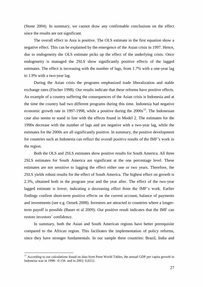
27

(Stone 2004). In summary, we cannot draw any confirmable conclusions on the effect

since the results are not significant.

The overall effect in Asia is positive. The OLS estimate in the first equation show a

negative effect. This can be explained by the emergence of the Asian crisis in 1997. Hence,

due to endogeneity the OLS estimate picks up the effect of the underlying crisis. Once

endogeneity is managed the 2SLS show significantly positive effects of the lagged

estimates. The effect is increasing with the number of lags, from 1.7% with a one-year lag

to 1.9% with a two-year lag.

During the Asian crisis the programs emphasized trade liberalization and stable

exchange rates (Fischer 1998). Our results indicate that these reforms have positive effects.

An example of a country suffering the consequences of the Asian crisis is Indonesia and at

the time the country had two different programs during this time. Indonesia had negative

economic growth rate in 1997-1998, while a positive during the 2000s12

. The Indonesian

case also seems to stand in line with the effects found in Model 2. The estimates for the

1990s decrease with the number of lags and are negative with a two-year lag, while the

estimates for the 2000s are all significantly positive. In summary, the positive development

for countries such as Indonesia can reflect the overall positive results of the IMF’s work in

the region.

Both the OLS and 2SLS estimates show positive results for South America. All three

2SLS estimates for South America are significant at the one percentage level. These

estimates are not sensitive to lagging the effect either one or two years. Therefore, the

2SLS yields robust results for the effect of South America. The highest effect on growth is

2.3%, obtained both in the program year and the year after. The effect of the two-year

lagged estimate is lower, indicating a decreasing effect from the IMF’s work. Earlier

findings confirm short-term positive effects on the current account, balance of payments

and investments (see e.g. Ozturk 2008). Investors are attracted to countries where a longer-

term payoff is possible (Bauer et al 2009). Our positive result indicates that the IMF can

restore investors’ confidence.

In summary, both the Asian and South American regions have better prerequisite

compared to the African region. This facilitates the implementation of policy reforms,

since they have stronger fundamentals. In our sample three countries: Brazil, India and

12

According to our calculations found on data from Penn World Tables, the annual GDP per capita growth in

Indonesia was in 1998: -0.156 and in 2002: 0,0212.

28

China, all part of the Brics13

, are often referred to as ‘growth miracles’ with a strong

positive development. By including these countries in our sample the mean growth rates in

the regions is raised. The overall positive results for the region can be explained by these

successful countries. The consistency in results concludes that the IMF is successful in

both Asia and South America.

13

The Brics consists of Brazil, Russia, India, China and South Africa. It is an association of fast-growing

economies (Desai 2013).

29

5. Conclusion

The success of the IMF’s lending arrangements has been subject to much debate. The IMF

began its work with a main focus on helping governments to restore balance of payments

problems but throughout time its purpose expanded beyond crisis management. Today, the

IMF works in both industrialized and developing countries, with the overall aim to increase

economic growth and living standards. In this thesis the short-term effects on growth of the

IMF’s lending arrangements in developing countries is analysed.

In theory, the IMF can influence economic growth via several channels. This thesis

identifies four: provide money through loan disbursements, work as an insurance for

investors, attach policy conditions to programs and monitor the world economy. Much

research has examined the effect of the IMF’s work on growth, but the results are

ambiguous. By performing a wide examination and analysing the different aspects of the

lending arrangements, it is possible to conclude that the IMF has been successful in

promoting growth. The effect on growth from an additional annual loan disbursement is

significantly positive. Though there are qualitative, historical and regional deviations.

One of the main contributions of this thesis is the analysis of the different kinds of

loans. Two lending arrangements, Stand-by arrangements (SBA) and Extended credit

facility (ECF) have significantly positive effects on growth. These programs also represent

the major directions of the IMF: providing monetary relief and structural development. The

results indicate that the IMF has been successful in achieving the aims of these policies in

the short-run.

Furthermore, the analysis shows a significantly positive result on growth when

controlling for the 1980s and 2000s. By dividing the data in shorter time periods we

capture the evolvement of the IMF’s work and can conclude a positive tendency. During

the late 1980s the focus of the IMF’s work changed towards promoting growth in

developing countries. New lending arrangements were established and the reach of the

policy conditions were widened. This process of adjustment is reflected in the positive

results on growth during the 2000s.

The IMF is successful in raising economic growth in Asia and South America.

Though, despite these positive results it is never possible to entirely protect countries from

the negative effects of external factors. The outburst of an economic crisis or a natural

disaster in one part of the world can influence the world economy. This can obstruct the

work of the IMF, even if programs are well-designed. These external factors highlight the

30

importance of surveillance of the member countries and the world economy. Furthermore,

the individual preconditions of the member countries cannot be completely accounted for.

This can be an explanation for the non-significant results for the African region, leading to

the conclusion that individual factors need to be taken into account. In general, immersing

to regional and local conditions can be of importance to get a deeper understanding of how

the IMF can promote growth.

Potential issues with endogenous variables are often highlighted in research on the

IMF’s work. In this thesis internal instruments are used, by adding the lagged dummy

variables for loan disbursements. This provides suitable instruments, but not perfect ones.

It is difficult to find efficient instruments and this has to be taken into account in the

analysis. In addition, a constraining factor is the availability and quality of data for

developing countries. A higher variance is expected in this data. Since some of the lending

arrangements are fairly new, few observations are available. This constraint on the data

hampers the possibility to draw confirmable conclusions and can explain some of the non-

significant results.

Economic growth is a wide subject and many explanatory factors can be included in

models. Though all models are simplifications of the real conditions observed. This means

that there is always a risk that important explanatory factors are left out, lowering the

power of explanation. Even though this thesis contributes to a wider knowledge on the

subject, unexplained factors remain. In spirit of Bird & Rowlands (2001), the nature of the

subject suggests that development of even wider models is useful to further investigate the

connection between the IMF and economic growth.

31

References

Abbott, Philip & Barnebeck Andersen, Thomas & Tarp, Finn (2009). “IMF and economic

reform in developing countries”, The Quarterly Review of Economics and Finance, vol. 50

(1), pp. 17-26. [Electronic]

http://www.sciencedirect.com/science/article/pii/S1062976909000970. (2013-04-25)

Atoyan, Ruben & Conway, Patrick, (2006). “Evaluating the impact of IMF programs: A

comparison of matching and instrumental-variable estimators”, The Review of

International Organizations, vol. 1 (2), pp. 99-124, [Electronic],

http://hdl.handle.net/10.1007/s11558-006-6612-2. (2013-04-24)

Barro, Robert, J. & Lee, Jong-Wha, (2003). “IMF Programs: Who Is Chosen and What Are

the Effects?”, Journal of Monetary Economics, vol. 52 (7), pp. 1245–1269. [Electronic]

http://dx.doi.org/10.1016/j.jmoneco.2005.04.003. (2013-04-12)

Barro, Robert J. & Lee, Jong-Wha, (2013), "Education Attainment for Population Aged 15

and Over", [Electronic] http://www.barrolee.com. (2013-04-12)

Barro, Robert, J. & Sala-i-Martin, Xavier, (2004). Economic Growth. 2nd

edition,

Cambridge: The MIT Press

Bauer, Molly & Cruz, Cesi & Graham, Benjamin, A. T., (2009) “Democracies Only: When

do IMF Agreements Serve as a Seal of Approval?”, Review of International Organizations,

vol. 7 (1), pp. 33-58, [Electronic] http://hdl.handle.net/10.1007/s11558-011-9122-9. (2013-

05-05)

Bird, Graham, (1996).“The International Monetary Fund and Developing Countries: A

Review of the Evidence and Policy Options”, International Organization, vol. 50 (3), pp.

477-511, [Electronic] http://www.jstor.org/stable/2704033. (2013-04-09)

Bird, Graham & Rowlands, Dane, (2001). “IMF lending: how is it affected by economic,

political and institutional factors?”, The Journal of Policy Reform, vol. 4 (3), pp. 243-270,

[Electronic] http://dx.doi.org/10.1080/13841280108523421. (2013-05-05)

Bloom, David,E., & Finlay, Jocelay, E., (2008). “Demographic Change and Economic

Growth in Asia”, PGDA Working Paper No. 41, The Program on the Global Demography

of Aging, September 2008 [Electronic]

http://www.hsph.harvard.edu/pgda/WorkingPapers/2008/PGDA_WP_41.pdf. (2013-05-20)

Boria, Claudio & White, William, (2004). “Whither monetary and financial stability? The

implications of evolving policy regimes”, BIS Working Papers No. 147, Bank of

International settlements, February 2004 [Electronic]

http://www.bis.org/publ/work147.pdf. (2013-05-24)

Brooks, Chris, (2008). Introductory Econometrics for finance. 2nd

edition, Cambridge:

Cambridge University Press

32

de Brouwer, Gordon, (2004). “The IMF and East Asia: A Changing Regional Financial

Architecture”, pp. 254-287 in Vines, David, Gilbert, Christopher, L., (ed.), The IMF and its

Critics: Reform of Global Financial Architecture. Cambridge: Cambridge University

Press. [Available] https://crawford.anu.edu.au/pdf/staff/gordon_debrouwer/GdB03-05.pdf.

(2013-05-19)

Conway, Patrick, (1994). “IMF lending programs: Participation and impact”, Journal of

Development Economics, vol. 45 (2), pp. 365-391, [Electronic]

http://dx.doi.org/10.1016/0304-3878(94)90038-8. (2013-04-25)

Dicks-Mireaux, Louis & Mecagni, Mauro & Schadler, Susan, (2000). “Evaluating the

effect of IMF lending to low-income countries”, Journal of Development Economics, vol.

61 (2), pp. 495-526, [Electronic]

http://www.development.wne.uw.edu.pl/uploads/Courses/dw_11_1.pdf. (2013-05-25)

Dougherty, Christopher, (2011). Introduction to econometrics. 4th

edition, Oxford: Oxford

University Press

Dreher, Axel, (2006). “IMF and Economic Growth: The Effects of Programs,

Loans, and Compliance with Conditionality”, World Development, vol. 34 (5), pp. 769–

788 [Electronic]. http://dx.doi.org/10.1016/j.worlddev.2005.11.002. (2013-04-09)

Easterly, William, (2005). “What did structural adjustment adjust? The association of

policies and growth with repeated IMF and World Bank adjustment loans”, Journal of

Development Economics, vol. 76 (1) pp. 1-22, [Electronic]

http://dx.doi.org/10.1016/j.jdeveco.2003.11.005. (2013-05-12)

Evrensel, Ayse, Y., (2002). “Effectiveness of IMF-supported stabilization programs in

developing countries”, Journal of International Money and Finance, vol. 21(5), pp. 565-

587, http://dx.doi.org/10.1016/S0261-5606(02)00010-4. (2013-04-09)

Evrensel, Ayse, Y. & Kim, Jong, Sung, (2006). “Macroeconomic policies and participation

in IMF programs”, Economic Systems, vol. 30 (3), pp. 264–281, [Electronic].

http://dx.doi.org/10.1016/j.ecosys.2006.05.002. (2013-04-09)

Fischer, Stanley, (1997). “Applied Economics in Action: IMF Programs”, The American

Economic Review, vol. 87 (2), pp.23-27, [Electronic]. http://www.jstor.org/stable/2950877.

(2013-04-24)

Fischer, Stanley, (1998). “The IMF and the Asian Crisis”, (Address by Stanley Fischer),

The International Monetary Fund, IMF external relations department, Los Angeles (1998-

03-20), [Electronic] http://www.imf.org/external/np/speeches/1998/032098.HTM. (2013-

04-24)

Hall, Robert, E., & Jones, Charles I., (1999). "Why Do Some Countries Produce So Much

More Output Per Worker Than Others?," The Quarterly Journal of Economics, vol. 114

(1), pp. 83-116, [Electronic]http://www.nber.org/papers/w6564.pdf. (2013-05-10)

Harris, Richard & Sollis, Robert, (2003). Applied times series modelling and forecasting.

1st edition, New York: John Wiley & Sons

33

Heston, Alan & Summers, Robert & Aten, Bettina, (2012) “Penn World Table Version

7.1”, Center for International Comparisons of Production, Income and Prices at the

University of Pennsylvania, [Electronic].

https://pwt.sas.upenn.edu/php_site/pwt71/pwt71_form_test.php. (2013-04-11)

Hill, R. Carter & Griffiths, William E. & Lim, Guay C., (2008). Principles of

Econometrics. 3rd

edition. Hoboken, N.J.: John Wiley & Sons

International Monetary Fund, (2013a). “IMF lending arrangements”. [Electronic].

http://www.imf.org/external/np/fin/tad/extarr1.aspx. (2013-04-09)

International Monetary Fund, (2013b). ”Factsheet: The IMF at a glance”. [Electronic]

http://www.imf.org/external/np/exr/facts/glance.htm. (2013-04-09)

International Monetary Fund, (2013d). “Factsheet: IMF lending”. [Electronic]

http://www.imf.org/external/np/exr/facts/howlend.htm. (2013-04-10)

International Monetary Fund, (2013f). “What we do”. [Electronic]

http://www.imf.org/external/about/whatwedo.htm. (2013-04-09)

International Monetary Fund, (2013g). “SDR Interest Rate, Rate of Remuneration, Rate of

Charge and Burden Sharing Adjustment”. [Electronic]

http://www.imf.org/external/np/tre/sdr/burden/2013/042913.htm. (2013-05-06)

International Monetary Fund, (2013h). “Factsheet: IMF Extended Credit Facility”.

[Electronic] http://www.imf.org/external/np/exr/facts/ecf.htm. (2013-05-10)

International Monetary Fund, (2013i). “IMF Lending Arrangements”. [Electronic]

http://www.imf.org/external/np/fin/tad/extarr1.aspx. (2013-05-10)

International Monetary Fund, (2004). “IMF Concessional Financing through the ESAF”.

[Electronic] http://www.imf.org/external/np/exr/facts/esaf.htm. 2013-04-10

International Monetary Fund, (2013j). “Membership”. [Electronic]

http://www.imf.org/external/about/members.htm. (2013-05-10)

International Monetary Fund, (2013k). “Factsheet: The Exogenous Shocks Facility - High

Access Component” (ESF - HAC)”. [Electronic]

http://www.imf.org/external/np/exr/facts/esf.htm. (2013-05-10)

International Monetary Fund, (2013l). “Debt and painful reforms (1982–89)” [Electronic]

http://www.imf.org/external/about/histdebt.htm. (2013-05-21)

International Monetary Fund, (2013m). “Societal Change for Eastern Europe and Asian

Upheaval (1990-2004)” [Electronic] http://www.imf.org/external/about/histcomm.htm.

(2013-05-21)

34

International Monetary Fund, (2001). “Structural Conditionality in Fund-Supported

Programs” [Electronic] http://www.imf.org/external/np/pdr/cond/2001/eng/struct/cond.pdf.

(2013-05-20)

International Monetary Fund, (2008) “Factsheet: How the IMF Helps to Resolve Balance

of Payments Difficulties” , [Electronic]

http://www.imf.org/external/np/exr/facts/crises.htm. (2013-05-20)

Inaternational Monetary Fund (2012), “IMF Annual Report 2012”, [Electronic]

http://www.imf.org/external/pubs/ft/ar/2012/eng/pdf/ar12_eng.pdf. (2013-05-20)

John, Jari & Knedlik, Tobias, (2011). “New IMF Lending Facilities and Financial Stability

in Emerging Markets”, Economic Analysis & Policy, vol. 41 (2), pp. 225-238, [Electronic]

http://www.eap-journal.com/archive/v41_i2_07-knedilk.pdf. (2013-05-19)

Jones, Charles I., (2002). Introduction to Economic Growth. 2nd

edition. New York: W.W

Norton & Company.

Jorra, Markus, (2011). “The Effect of IMF Lending on the Probability of Sovereign Debt

Crises”, Journal of International Money and Finance, vol. 31 (4), pp. 709-725,

[Electronic] http://www.uni-marburg.de/fb02/makro/forschung/magkspapers/26-

2010_jorra.pdf. (2013-05-05)

Killick, Tony & Malik, Moazzam & Manuel, Marcus, (1992). “What Can We Know about

the Effects of IMF Programmes?”, The World Economy, vol. 15 (5), pp 575–598,

[Electronic] http://onlinelibrary.wiley.com.ludwig.lub.lu.se/doi/10.1111/j.1467-

9701.1992.tb00538.x/pdf. (2013-05-06)

Marchesi, Silvia & Sirtori, Emanuela, (2011). “Is two better than one? The effects of IMF

and World Bank interaction on growth”, The Review of International Organizations, vol. 6

(3), pp. 287-306, [Electronic]

http://dipeco.economia.unimib.it/corsi/739/lezioni/marchesisirtoririo.pdf. (2013-04-09)

Meltzer, Allan (1999). “What’s wrong with the IMF? What would be better?”. The

independent review, vol. 4 (2), pp. 201-215, [Electronic]

http://www.independent.org/pdf/tir/tir_04_2_meltzer.pdf. (2013-04-25)

Nunnenkamp, Peter, (1998). “Dealing with the Asian crisis: IMF conditionality and

implications in Asia and beyond“, Intereconomics, vol. 33 (2), pp. 64-72, [Electronic]

http://hdl.handle.net/10419/1742. (2013-05-19)

Ozturk, Ilhan, (2008). “Evaluating the Macroeconomic Impacts of IMF Programmes in

Latin America, 1975-2004: A GEE Analysis”, South African Journal of Economic and

Management Sciences, vol. 11 (2), pp.190-202, [Electronic]

http://www.sajems.org/index.php/sajems/article/view/308/119. (2013-05-05)

Presbitero, Andera F. & Zazzaro, Alberto, (2012). “IMF Lending in Times of Crisis:

Political Influences and Crisis Prevention”, World Development, vol. 40 (10), pp. 1944-

1969, [Electronic] http://dx.doi.org/10.1016/j.worlddev.2012.04.009. (2013-04-09)

35

Przeworski, Adam & Vreeland, James Raymond, (2000). “The effect of IMF programs on

economic growth”, Journal of Development Economics, vol. 62 (2), pp. 385–421

[Electronic]. http://dx.doi.org/10.1016/S0304-3878(00)00090-0. (2013-04-22)

Reichmann, T.M. & Stillson, R.T., (1978). “Experience with programs of balance of

payments adjustment: stand-by arrangements in the highest tranches, 1963–72”. IMF Staff

Papers 25, pp. 292–310. [Electronic]. http://www.palgrave-

journals.com/imfsp/journal/v25/n2/pdf/imfsp197811a.pdf. (2013-05-05)

Rodrik, Dani, (2003). ”Growth strategies”, NBER Working Paper No. 10050, National

Bureau of Economic Research, October 2003 [Electronic].

http://www.nber.org/papers/w10050. (2013-04-24)

Stone, Randall, W., (2004). “The Political Economy of IMF Lending in Africa”, American

Political Science Review, vol. 98 (4), pp. 577-591, [Electronic]

http://www.jstor.org/stable/4145326. (2013-05-05)

Stephey, M.J. (2008). “A brief history of the Bretton Woods System”, Time Business &

Money, Oct. 21, 2008 [Electronic]

http://www.time.com/time/business/article/0,8599,1852254,00.html. (2013-05-20)

University of Pennsylvania, (2008). “Penn World Table: Study documentation”

[Electronic] http://idsc.iza.org/metadata/PDF/365.pdf. (2013-04-20)

The World Bank, (2013a). “Country and Lending groups” [Electronic].

http://data.worldbank.org/about/country-classifications/country-and-lending-groups.

(2013-04-24)

The World Bank, (2013b), “Fertility rate, total (births per woman)”. [Electronic].

http://data.worldbank.org/indicator/SP.DYN.TFRT.IN. (2013-04-24)

The World Bank, (2013c), “Life expectancy at birth, total (years)”. [Electronic].

http://data.worldbank.org/indicator/SP.DYN.LE00.IN. (2013-04-24)

Verbeek, Marno, (2008), A Guide to Modern Econometrics. 3rd

edition. Chichester: John

Wiley & Sons Lt

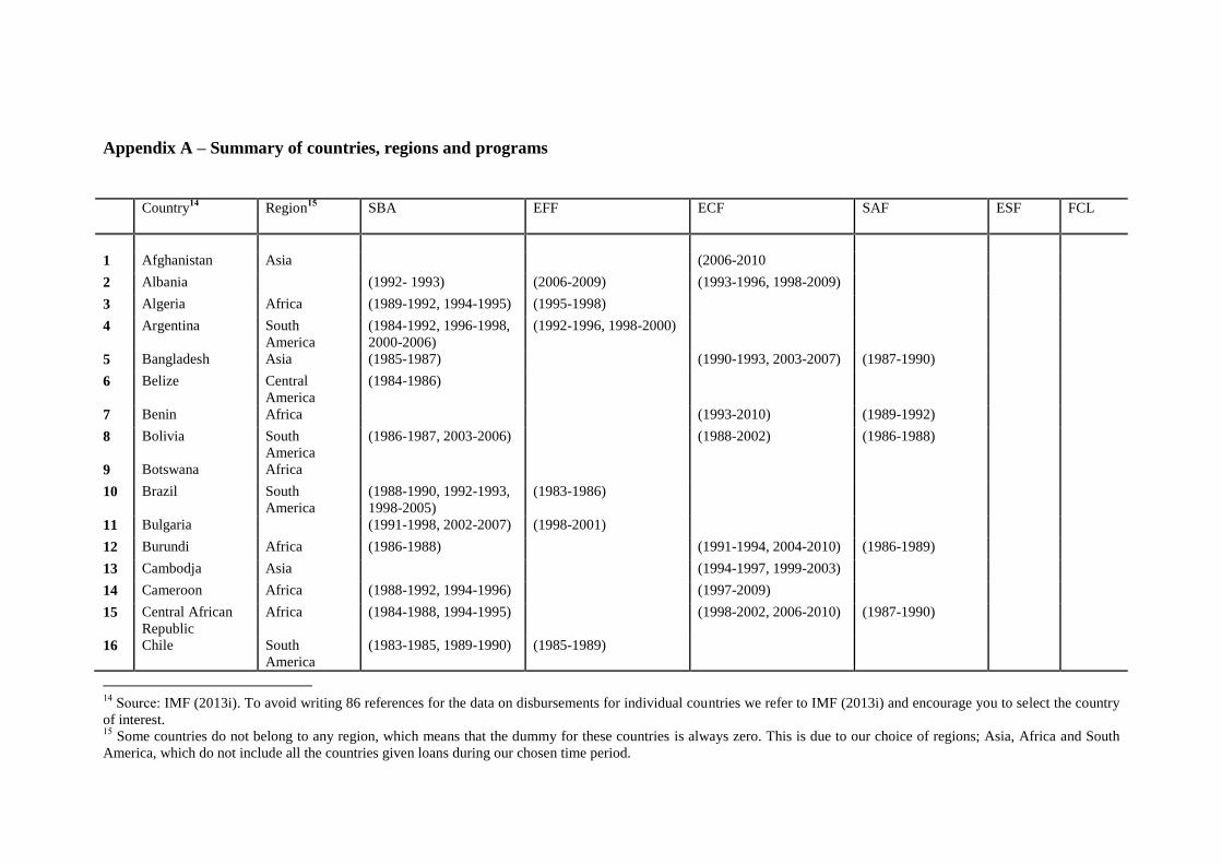
Appendix A – Summary of countries, regions and programs

Country14

Region15

SBA EFF ECF SAF ESF FCL

1 Afghanistan Asia (2006-2010

2 Albania (1992- 1993) (2006-2009) (1993-1996, 1998-2009)

3 Algeria Africa (1989-1992, 1994-1995) (1995-1998)

4 Argentina South

America

(1984-1992, 1996-1998,

2000-2006)

(1992-1996, 1998-2000)

5 Bangladesh Asia (1985-1987) (1990-1993, 2003-2007) (1987-1990)

6 Belize Central

America

(1984-1986)

7 Benin Africa (1993-2010) (1989-1992)

8 Bolivia South

America

(1986-1987, 2003-2006) (1988-2002) (1986-1988)

9 Botswana Africa

10 Brazil South

America

(1988-1990, 1992-1993,

1998-2005)

(1983-1986)

11 Bulgaria (1991-1998, 2002-2007) (1998-2001)

12 Burundi Africa (1986-1988) (1991-1994, 2004-2010) (1986-1989)

13 Cambodja Asia (1994-1997, 1999-2003)

14 Cameroon Africa (1988-1992, 1994-1996) (1997-2009)

15 Central African

Republic

Africa (1984-1988, 1994-1995) (1998-2002, 2006-2010) (1987-1990)

16 Chile South

America

(1983-1985, 1989-1990) (1985-1989)

14

Source: IMF (2013i). To avoid writing 86 references for the data on disbursements for individual countries we refer to IMF (2013i) and encourage you to select the country

of interest. 15

Some countries do not belong to any region, which means that the dummy for these countries is always zero. This is due to our choice of regions; Asia, Africa and South

America, which do not include all the countries given loans during our chosen time period.

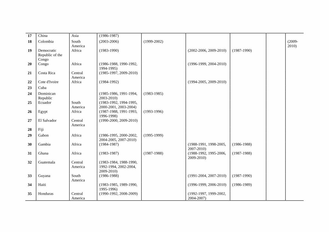
17 China Asia (1986-1987)

18 Colombia South

America

(2003-2006) (1999-2002) (2009-

2010)

19 Democratic

Republic of the

Congo

Africa (1983-1990) (2002-2006, 2009-2010) (1987-1990)

20 Congo Africa (1986-1988, 1990-1992,

1994-1995)

(1996-1999, 2004-2010)

21 Costa Rica Central

America

(1985-1997, 2009-2010)

22 Cote d'Ivoire Africa (1984-1992) (1994-2005, 2009-2010)

23 Cuba

24 Dominican

Republic

(1985-1986, 1991-1994,

2003-2010)

(1983-1985)

25 Ecuador South

America

(1983-1992, 1994-1995,

2000-2001, 2003-2004)

26 Egypt Africa (1987-1988, 1991-1993,

1996-1998)

(1993-1996)

27 El Salvador Central

America

(1990-2000, 2009-2010)

28 Fiji

29 Gabon Africa (1986-1995, 2000-2002,

2004-2005, 2007-2010)

(1995-1999)

30 Gambia Africa (1984-1987) (1988-1991, 1998-2005,

2007-2010)

(1986-1988)

31 Ghana Africa (1983-1987) (1987-1988) (1988-1992, 1995-2006,

2009-2010)

(1987-1988)

32 Guatemala Central

America

(1983-1984, 1988-1990,

1992-1994, 2002-2004,

2009-2010)

33 Guyana South

America

(1986-1988) (1991-2004, 2007-2010) (1987-1990)

34 Haiti (1983-1985, 1989-1990,

1995-1996)

(1996-1999, 2006-2010) (1986-1989)

35 Honduras Central

America

(1990-1992, 2008-2009) (1992-1997, 1999-2002,

2004-2007)

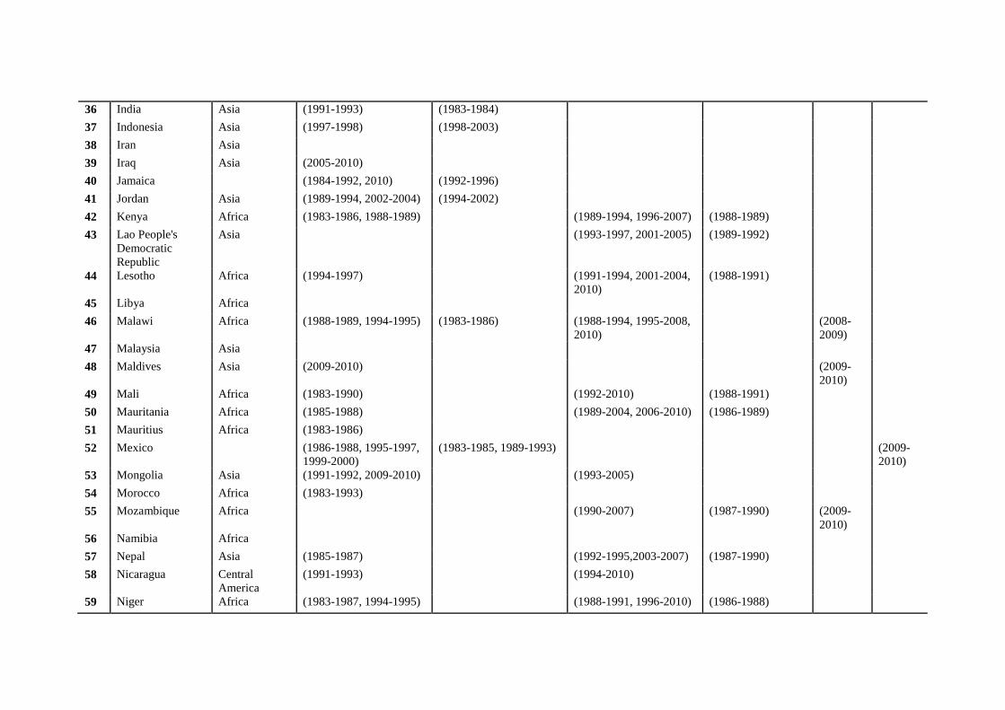
36 India Asia (1991-1993) (1983-1984)

37 Indonesia Asia (1997-1998) (1998-2003)

38 Iran Asia

39 Iraq Asia (2005-2010)

40 Jamaica (1984-1992, 2010) (1992-1996)

41 Jordan Asia (1989-1994, 2002-2004) (1994-2002)

42 Kenya Africa (1983-1986, 1988-1989) (1989-1994, 1996-2007) (1988-1989)

43 Lao People's

Democratic

Republic

Asia (1993-1997, 2001-2005) (1989-1992)

44 Lesotho Africa (1994-1997) (1991-1994, 2001-2004,

2010)

(1988-1991)

45 Libya Africa

46 Malawi Africa (1988-1989, 1994-1995) (1983-1986) (1988-1994, 1995-2008,

2010)

(2008-

2009)

47 Malaysia Asia

48 Maldives Asia (2009-2010) (2009-

2010)

49 Mali Africa (1983-1990) (1992-2010) (1988-1991)

50 Mauritania Africa (1985-1988) (1989-2004, 2006-2010) (1986-1989)

51 Mauritius Africa (1983-1986)

52 Mexico (1986-1988, 1995-1997,

1999-2000)

(1983-1985, 1989-1993) (2009-

2010)

53 Mongolia Asia (1991-1992, 2009-2010) (1993-2005)

54 Morocco Africa (1983-1993)

55 Mozambique Africa (1990-2007) (1987-1990) (2009-

2010)

56 Namibia Africa

57 Nepal Asia (1985-1987) (1992-1995,2003-2007) (1987-1990)

58 Nicaragua Central

America

(1991-1993) (1994-2010)

59 Niger Africa (1983-1987, 1994-1995) (1988-1991, 1996-2010) (1986-1988)

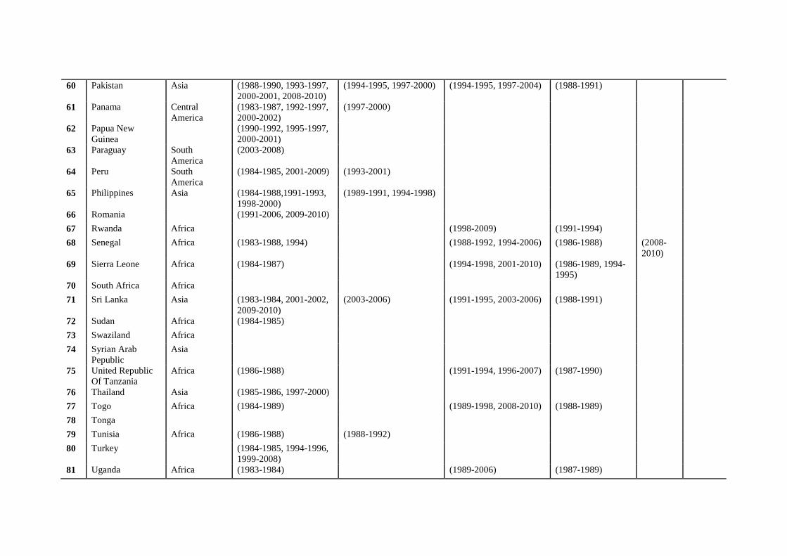
60 Pakistan Asia (1988-1990, 1993-1997,

2000-2001, 2008-2010)

(1994-1995, 1997-2000) (1994-1995, 1997-2004) (1988-1991)

61 Panama Central

America

(1983-1987, 1992-1997,

2000-2002)

(1997-2000)

62 Papua New

Guinea

(1990-1992, 1995-1997,

2000-2001)

63 Paraguay South

America

(2003-2008)

64 Peru South

America

(1984-1985, 2001-2009) (1993-2001)

65 Philippines Asia (1984-1988,1991-1993,

1998-2000)

(1989-1991, 1994-1998)

66 Romania (1991-2006, 2009-2010)

67 Rwanda Africa (1998-2009) (1991-1994)

68 Senegal Africa (1983-1988, 1994) (1988-1992, 1994-2006) (1986-1988) (2008-

2010)

69 Sierra Leone Africa (1984-1987) (1994-1998, 2001-2010) (1986-1989, 1994-

1995)

70 South Africa Africa

71 Sri Lanka Asia (1983-1984, 2001-2002,

2009-2010)

(2003-2006) (1991-1995, 2003-2006) (1988-1991)

72 Sudan Africa (1984-1985)

73 Swaziland Africa

74 Syrian Arab

Pepublic

Asia

75 United Republic

Of Tanzania

Africa (1986-1988) (1991-1994, 1996-2007) (1987-1990)

76 Thailand Asia (1985-1986, 1997-2000)

77 Togo Africa (1984-1989) (1989-1998, 2008-2010) (1988-1989)

78 Tonga

79 Tunisia Africa (1986-1988) (1988-1992)

80 Turkey (1984-1985, 1994-1996,

1999-2008)

81 Uganda Africa (1983-1984) (1989-2006) (1987-1989)

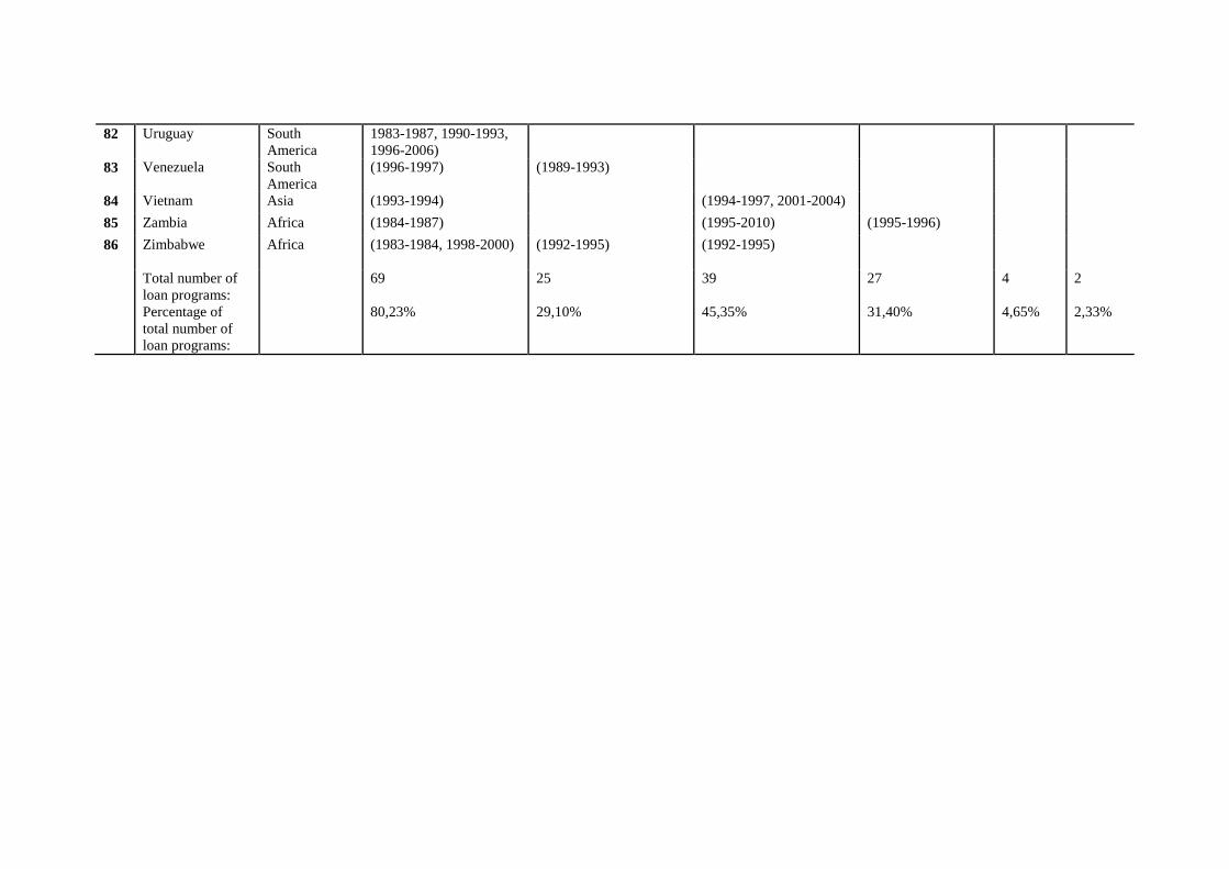
82 Uruguay South

America

1983-1987, 1990-1993,

1996-2006)

83 Venezuela South

America

(1996-1997) (1989-1993)

84 Vietnam Asia (1993-1994) (1994-1997, 2001-2004)

85 Zambia Africa (1984-1987) (1995-2010) (1995-1996)

86 Zimbabwe Africa (1983-1984, 1998-2000)

(1992-1995) (1992-1995)

Total number of

loan programs:

69

25 39 27 4 2

Percentage of

total number of

loan programs:

80,23% 29,10% 45,35% 31,40% 4,65% 2,33%

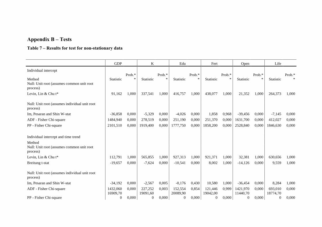
Appendix B – Tests

Table 7 – Results for test for non-stationary data

GDP K Edu Fert Open Life

Individual intercept

Method Statistic

Prob.*

* Statistic

Prob.*

* Statistic

Prob.*

* Statistic

Prob.*

* Statistic

Prob.*

* Statistic

Prob.*

*

Null: Unit root (assumes common unit root

process)

Levin, Lin & Chu t* 91,162 1,000 337,541 1,000 416,757 1,000 438,077 1,000 21,352 1,000 264,373 1,000

Null: Unit root (assumes individual unit root

process)

Im, Pesaran and Shin W-stat -36,858 0,000 -5,329 0,000 -4,026 0,000 1,858 0,968 -39,456 0,000 -7,145 0,000

ADF - Fisher Chi-square 1484,940 0,000 278,519 0,000 251,190 0,000 251,370 0,000 1631,700 0,000 412,027 0,000

PP - Fisher Chi-square 2101,510 0,000 1919,400 0,000 1777,750 0,000 1858,200 0,000 2528,840 0,000 1846,630 0,000

Individual intercept and time trend

Method

Null: Unit root (assumes common unit root

process)

Levin, Lin & Chu t* 112,791 1,000 565,855 1,000 927,313 1,000 921,371 1,000 32,381 1,000 630,656 1,000

Breitung t-stat -19,657 0,000 -7,624 0,000 -10,541 0,000 8,002 1,000 -14,126 0,000 9,559 1,000

Null: Unit root (assumes individual unit root

process)

Im, Pesaran and Shin W-stat -34,192 0,000 -2,567 0,005 -0,176 0,430 10,580 1,000 -36,454 0,000 8,284 1,000

ADF - Fisher Chi-square 1432,060 0,000 227,252 0,003 152,554 0,854 121,446 0,999 1421,970 0,000 693,010 0,000

PP - Fisher Chi-square

16909,70

0 0,000

19091,60

0 0,000

20089,90

0 0,000

19042,00

0 0,000

11440,70

0 0,000

18774,70

0 0,000

Non-stationary data can create a false correlation, as variables growth with time. By using

unit root tests a non-time dependent correlation between the variables can be detected and

the null-hypothesis (contains a unit root process) can be rejected (Brooks 2008, p. 327).

The results of the tests are shown in Table 7, where the upper part of the table shows the

results when the test are allowing for an individual intercept, while the lower part shows

the results when the tests are allows for both an individual intercept and a time trend.

The LLC (Levin, Lin and Chu) test assumes a common unit root process, and is more

restrictive than the other tests performed. This test assumes an alternative hypothesis

saying that all the series must be stationary to be able to reject the null-hypothesis,

compared to the other tests where only one series need to be stationary (Harris & Sollis

2003, p. 191-193). Evaluating the results of this test using the p-values, the null-hypothesis

cannot be rejected for any of the variables. Due to the restrictive characteristics of this test

the results are complemented with other tests.

The other three tests have a null-hypothesis assuming individual unit-root process.

The IPS (Im, Pesaran and Shin) test rejects the null-hypothesis for all the variables, except

fertility rate. The ADF (Augmented Dickey Fuller) and PP (Phillips-Perron) tests reject the

null hypothesis for all the variables at the one percentage level (Harris & Sollis 2003, p.

196, Brooks 2008, p. 330-331).

When the tests are allowing for individual intercepts and time trends, the LLC test

again shows the same results and is not able to reject the null-hypothesis for any of the

variables. Using the UB (Breitung) test a common unit root process is assumed and the

null-hypothesis is rejected for all the variables, except for fertility rate and life expectancy.

The IPS test rejects the null-hypothesis for GDP per capita, the stock of capital and

openness, but not for education, fertility rate and life expectancy. The ADF test rejects all

the null-hypothesis for all the variables, except education and fertility rate. Finally, the PP

test rejects the null hypothesis for all the variables.

In summary, the results three of the variables; GDP per capita, the capital stock and

openness, are concluded to be stationary according to all tests, except for the LLC and UB

tests. The deviating results of the UB test can be explained by the fact that this test only

involves a constant (i.e. no fixed effects) (Harris & Sollis 2003, p. 195). While the

restrictive character of the LLC test and its consistent inability to reject the null-hypothesis

for any of the variables yields implausible results. For the other variables; the fertility rate

and education, the tests yield inconclusive results. This can be due to the different

assumptions of the tests. Both of the PP tests reject the null-hypothesis for all the variables,

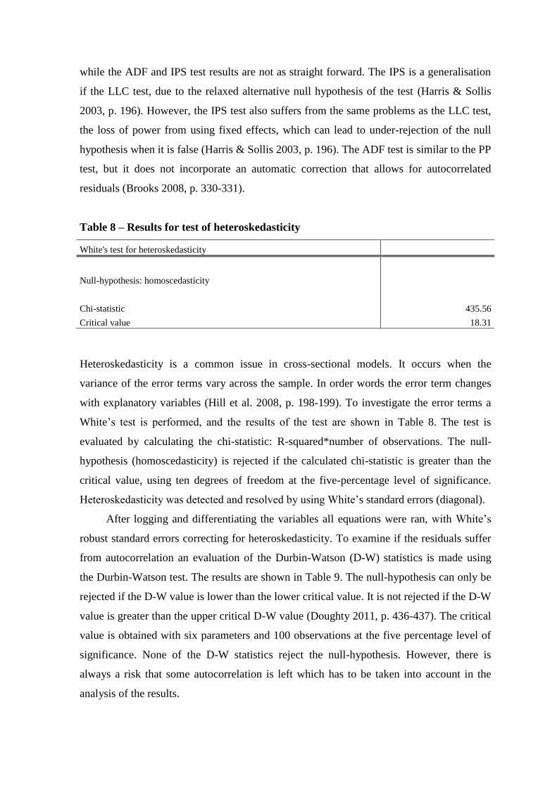
while the ADF and IPS test results are not as straight forward. The IPS is a generalisation

if the LLC test, due to the relaxed alternative null hypothesis of the test (Harris & Sollis

2003, p. 196). However, the IPS test also suffers from the same problems as the LLC test,

the loss of power from using fixed effects, which can lead to under-rejection of the null

hypothesis when it is false (Harris & Sollis 2003, p. 196). The ADF test is similar to the PP

test, but it does not incorporate an automatic correction that allows for autocorrelated

residuals (Brooks 2008, p. 330-331).

Table 8 – Results for test of heteroskedasticity

White's test for heteroskedasticity

Null-hypothesis: homoscedasticity

Chi-statistic 435.56

Critical value 18.31

Heteroskedasticity is a common issue in cross-sectional models. It occurs when the

variance of the error terms vary across the sample. In order words the error term changes

with explanatory variables (Hill et al. 2008, p. 198-199). To investigate the error terms a

White’s test is performed, and the results of the test are shown in Table 8. The test is

evaluated by calculating the chi-statistic: R-squared*number of observations. The null-

hypothesis (homoscedasticity) is rejected if the calculated chi-statistic is greater than the

critical value, using ten degrees of freedom at the five-percentage level of significance.

Heteroskedasticity was detected and resolved by using White’s standard errors (diagonal).

After logging and differentiating the variables all equations were ran, with White’s

robust standard errors correcting for heteroskedasticity. To examine if the residuals suffer

from autocorrelation an evaluation of the Durbin-Watson (D-W) statistics is made using

the Durbin-Watson test. The results are shown in Table 9. The null-hypothesis can only be

rejected if the D-W value is lower than the lower critical value. It is not rejected if the D-W

value is greater than the upper critical D-W value (Doughty 2011, p. 436-437). The critical

value is obtained with six parameters and 100 observations at the five percentage level of

significance. None of the D-W statistics reject the null-hypothesis. However, there is

always a risk that some autocorrelation is left which has to be taken into account in the

analysis of the results.

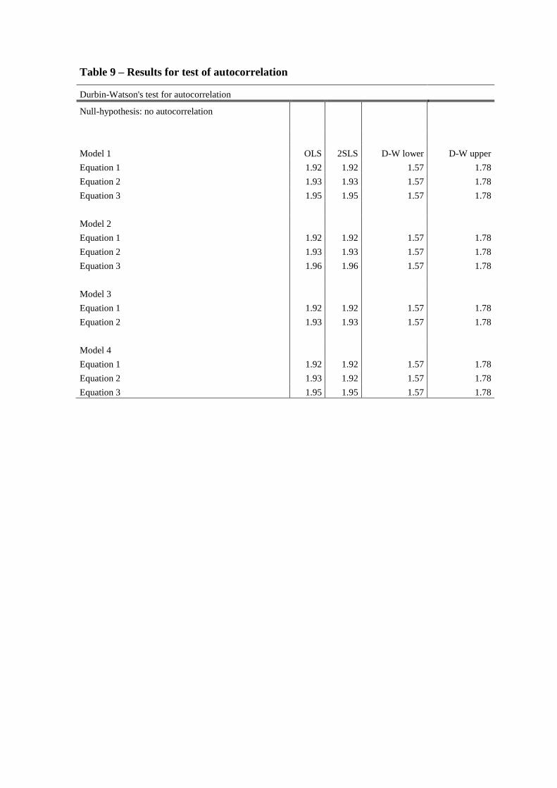
Table 9 – Results for test of autocorrelation

Durbin-Watson's test for autocorrelation

Null-hypothesis: no autocorrelation

Model 1 OLS 2SLS D-W lower D-W upper

Equation 1 1.92 1.92 1.57 1.78

Equation 2 1.93 1.93 1.57 1.78

Equation 3 1.95 1.95 1.57 1.78

Model 2

Equation 1 1.92 1.92 1.57 1.78

Equation 2 1.93 1.93 1.57 1.78

Equation 3 1.96 1.96 1.57 1.78

Model 3

Equation 1 1.92 1.92 1.57 1.78

Equation 2 1.93 1.93 1.57 1.78

Model 4

Equation 1 1.92 1.92 1.57 1.78

Equation 2 1.93 1.92 1.57 1.78

Equation 3 1.95 1.95 1.57 1.78

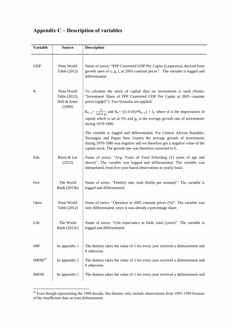
Appendix C – Description of variables

Variable Source Description

GDP

Penn World

Table (2012)

Name of series: “PPP Converted GDP Per Capita (Laspeyres), derived from

growth rates of c, g, i, at 2005 constant prices”. The variable is logged and

differentiated.

K Penn World

Table (2012),

Hall & Jones

(1999)

To calculate the stock of capital data on investments is used (Series:

“Investment Share of PPP Converted GDP Per Capita at 2005 constant

prices [rgdpl]”). Two formulas are applied:

=

and = ((1-0.05)* ) + where d is the depreciation of

capital which is set at 5% and is the average growth rate of investments

during 1970-1980.

The variable is logged and differentiated. For Central African Republic,

Nicaragua and Papua New Guinea the average growth of investments

during 1970-1980 was negative and we therefore got a negative value of the

capital stock. The growth rate was therefore corrected to 0.

Edu Barro & Lee

(2013)

Name of series: “Avg. Years of Total Schooling (15 years of age and

above)”. The variable was logged and differentiated. The variable was

interpolated, from five-year based observations to yearly basis.

Fert The World

Bank (2013b)

Name of series: “Fertility rate, total (births per woman)”. The variable is

logged and differentiated.

Open Penn World

Table (2012)

Name of series: “Openness at 2005 constant prices (%)”. The variable was

only differentiated, since it was already a percentage share.

Life The World

Bank (2013c)

Name of series: “Life expectancy at birth, total (years)”. The variable is

logged and differentiated.

IMF Se appendix 1 The dummy takes the value of 1 for every year received a disbursement and

0 otherwise.

IMF8016

Se appendix 1 The dummy takes the value of 1 for every year received a disbursement and

0 otherwise.

IMF90 Se appendix 1 The dummy takes the value of 1 for every year received a disbursement and

16

Even though representing the 1980 decade, this dummy only include observations from 1983-1989 because

of the insufficient data on loan disbursement.

0 otherwise.

IMF00 Se appendix 1 The dummy takes the value of 1 for every year received a disbursement and

0 otherwise.

SBA Se appendix 1 The dummy takes the value of 1 for every year received a disbursement and

0 otherwise.

EFF Se appendix1 The dummy takes the value of 1 for every year received a disbursement and

0 otherwise.

ECF Se appendix 1 The dummy takes the value of 1 for every year received a disbursement and

0 otherwise.

SAF Se appendix 1 The dummy takes the value of 1 for every year received a disbursement and

0 otherwise.

ESF Se appendix 1 The dummy takes the value of 1 for every year received a disbursement and

0 otherwise.

FCL Se appendix 1 The dummy takes the value of 1 for every year received a disbursement and

0 otherwise.

Africa Se appendix 1 The dummy takes the value of 1 for every year received a disbursement and

0 otherwise.

Asia Se appendix 1 The dummy takes the value of 1 for every year received a disbursement and

0 otherwise.

South

America

Se appendix 1 The dummy takes the value of 1 for every year received a disbursement and

0 otherwise.

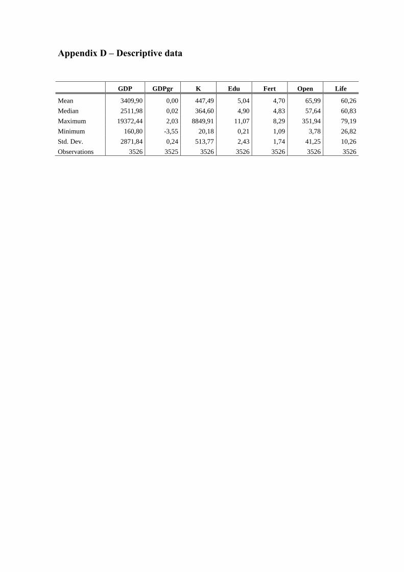
Appendix D – Descriptive data

GDP GDPgr K Edu Fert Open Life

Mean 3409,90 0,00 447,49 5,04 4,70 65,99 60,26

Median 2511,98 0,02 364,60 4,90 4,83 57,64 60,83

Maximum 19372,44 2,03 8849,91 11,07 8,29 351,94 79,19

Minimum 160,80 -3,55 20,18 0,21 1,09 3,78 26,82

Std. Dev. 2871,84 0,24 513,77 2,43 1,74 41,25 10,26

Observations 3526 3525 3526 3526 3526 3526 3526

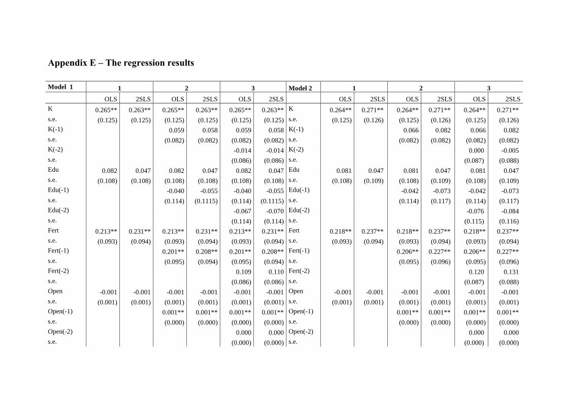
Appendix E – The regression results

Model 1 1 2 3 Model 2 1 2 3

OLS 2SLS OLS 2SLS OLS 2SLS

OLS 2SLS OLS 2SLS OLS 2SLS

K 0.265** 0.263** 0.265** 0.263** 0.265** 0.263** K 0.264** 0.271** 0.264** 0.271** 0.264** 0.271**

s.e. (0.125) (0.125) (0.125) (0.125) (0.125) (0.125) s.e. (0.125) (0.126) (0.125) (0.126) (0.125) (0.126)

K(-1) 0.059 0.058 0.059 0.058 K(-1)

0.066 0.082 0.066 0.082

s.e. (0.082) (0.082) (0.082) (0.082) s.e. (0.082) (0.082) (0.082) (0.082)

K(-2) -0.014 -0.014 K(-2) 0.000 -0.005

s.e. (0.086) (0.086) s.e. (0.087) (0.088)

Edu 0.082 0.047 0.082 0.047 0.082 0.047 Edu 0.081 0.047 0.081 0.047 0.081 0.047

s.e. (0.108) (0.108) (0.108) (0.108) (0.108) (0.108) s.e. (0.108) (0.109) (0.108) (0.109) (0.108) (0.109)

Edu(-1) -0.040 -0.055 -0.040 -0.055 Edu(-1) -0.042 -0.073 -0.042 -0.073

s.e. (0.114) (0.1115) (0.114) (0.1115) s.e. (0.114) (0.117) (0.114) (0.117)

Edu(-2) -0.067 -0.070 Edu(-2) -0.076 -0.084

s.e. (0.114) (0.114) s.e. (0.115) (0.116)

Fert 0.213** 0.231** 0.213** 0.231** 0.213** 0.231** Fert 0.218** 0.237** 0.218** 0.237** 0.218** 0.237**

s.e. (0.093) (0.094) (0.093) (0.094) (0.093) (0.094) s.e. (0.093) (0.094) (0.093) (0.094) (0.093) (0.094)

Fert(-1) 0.201** 0.208** 0.201** 0.208** Fert(-1) 0.206** 0.227** 0.206** 0.227**

s.e. (0.095) (0.094) (0.095) (0.094) s.e. (0.095) (0.096) (0.095) (0.096)

Fert(-2) 0.109 0.110 Fert(-2) 0.120 0.131

s.e. (0.086) (0.086) s.e. (0.087) (0.088)

Open -0.001 -0.001 -0.001 -0.001 -0.001 -0.001 Open -0.001 -0.001 -0.001 -0.001 -0.001 -0.001

s.e. (0.001) (0.001) (0.001) (0.001) (0.001) (0.001) s.e. (0.001) (0.001) (0.001) (0.001) (0.001) (0.001)

Open(-1) 0.001** 0.001** 0.001** 0.001** Open(-1) 0.001** 0.001** 0.001** 0.001**

s.e. (0.000) (0.000) (0.000) (0.000) s.e. (0.000) (0.000) (0.000) (0.000)

Open(-2) 0.000 0.000 Open(-2) 0.000 0.000

s.e. (0.000) (0.000) s.e. (0.000) (0.000)

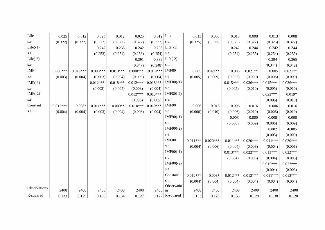
Life 0.025 0.012 0.025 0.012 0.025 0.012 Life 0.013 0.008 0.013 0.008 0.013 0.008

s.e. (0.322) (0.322) (0.322) (0.322) (0.322) (0.322) s.e. (0.325) (0.327) (0.325) (0.327) (0.325) (0.327)

Life(-1) 0.242 0.236 0.242 0.236 Life(-1) 0.242 0.244 0.242 0.244

s.e. (0.253) (0.254) (0.253) (0.254) s.e. (0.254) (0.255) (0.254) (0.255)

Life(-2) 0.391 0.389 Life(-2) 0.394 0.365

s.e. (0.347) (0.348) s.e. (0.344) (0.342)

IMF 0.008*** 0.019*** 0.008*** 0.019*** 0.008*** 0.019*** IMF80 0.005 0.021** 0.005 0.021** 0.005 0.021**

s.e. (0.003) (0.004) (0.003) (0.004) (0.003) (0.004) s.e. (0.005) (0.009) (0.005) (0.009) (0.005) (0.009)

IMF(-1) 0.012*** 0.018*** 0.012*** 0.018*** IMF80(-1) 0.015*** 0.036*** 0.015*** 0.036***

s.e. (0.003) (0.004) (0.003) (0.004) s.e. (0.005) (0.010) (0.005) (0.010)

IMF(-2) 0.012*** 0.013*** IMF80(-2) 0.022*** 0.019*

s.e. (0.003) (0.005) s.e. (0.006) (0.010)

Constant 0.012*** 0.008* 0.011*** 0.009** 0.010*** 0.010*** IMF90 0.006 0.016 0.006 0.016 0.006 0.016

s.e. (0.004) (0.004) (0.003) (0.004) (0.003) (0.004) s.e. (0.006) (0.010) (0.006) (0.010) (0.006) (0.010)

IMF90(-1) 0.008 0.000 0.008 0.000

s.e. (0.006) (0.009) (0.006) (0.009)

IMF90(-2) 0.002 -0.005

s.e. (0.005) (0.009)

IMF00 0.011*** 0.020*** 0.011*** 0.020*** 0.011*** 0.020***

s.e. (0.004) (0.006) (0.004) (0.006) (0.004) (0.006)

IMF00(-1) 0.013*** 0.022*** 0.013*** 0.022***

s.e. (0.004) (0.006) (0.004) (0.006)

IMF00(-2) 0.015*** 0.027***

s.e. (0.004) (0.006)

Constant 0.012*** 0.008* 0.012*** 0.012*** 0.011*** 0.012***

s.e. (0.004) (0.004) (0.004) (0.004) (0.004) (0.004)

Observations 2408 2408 2408 2408 2408 2408

Observatio

ns 2408 2408 2408 2408 2408 2408

R-squared 0.133 0.129 0.135 0.134 0.127 0.127 R-squared 0.133 0.129 0.135 0.128 0.130 0.128

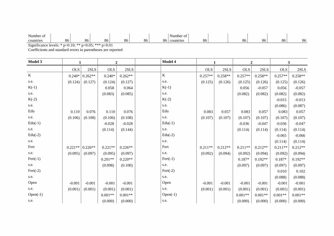
Number of

countries 86 86 86 86 86 86

Number of

countries 86 86 86 86 86

Significance levels: * p<0.10; ** p<0.05; *** p<0.01

Coefficients and standard errors in parentheses are reported

Model 3 1 2 Model 4 1 2 3

OLS 2SLS OLS 2SLS OLS 2SLS OLS 2SLS OLS 2SLS

K 0.240* 0.262** 0.240* 0.262** K 0.257** 0.258** 0.257** 0.258** 0.257** 0.258**

s.e. (0.124) (0.127) (0.124) (0.127) s.e. (0.125) (0.126) (0.125) (0.126) (0.125) (0.126)

K(-1) 0.058 0.064 K(-1) 0.056 -0.057 0.056 -0.057

s.e. (0.083) (0.085) s.e. (0.082) (0.082) (0.082) (0.082)

K(-2) K(-2) -0.015 -0.013

s.e. s.e. (0.086) (0.087)

Edu 0.110 0.076 0.110 0.076 Edu 0.083 0.057 0.083 0.057 0.083 0.057

s.e. (0.106) (0.108) (0.106) (0.108) s.e. (0.107) (0.107) (0.107) (0.107) (0.107) (0.107)

Edu(-1) -0.028 -0.028 Edu(-1) -0.036 -0.047 -0.036 -0.047

s.e. (0.114) (0.144) s.e. (0.114) (0.114) (0.114) (0.114)

Edu(-2) Edu(-2) -0.065 -0.066

s.e. s.e. (0.114) (0.114)

Fert 0.221** 0.226** 0.221** 0.226** Fert 0.211** 0.212** 0.211** 0.212** 0.211** 0.212**

s.e. (0.095) (0.097) (0.095) (0.097) s.e. (0.092) (0.094) (0.092) (0.094) (0.092) (0.094)

Fert(-1) 0.201** 0.220** Fert(-1) 0.187* 0.192** 0.187* 0.192**

s.e. (0.098) (0.100) s.e. (0.097) (0.097) (0.097) (0.097)

Fert(-2) Fert(-2) 0.010 0.102

s.e. s.e. (0.088) (0.088)

Open -0.001 -0.001 -0.001 -0.001 Open -0.001 -0.001 -0.001 -0.001 -0.001 -0.001

s.e. (0.001) (0.001) (0.001) (0.001) s.e. (0.001) (0.001) (0.001) (0.001) (0.001) (0.001)

Open(-1) 0.001** 0.001** Open(-1) 0.001** 0.001** 0.001** 0.001**

s.e. (0.000) (0.000) s.e. (0.000) (0.000) (0.000) (0.000)

Open(-2) Open(-2) 0.000 0.000

s.e. s.e. (0.000) (0.000)

Life -0.016 0.010 -0.016 0.010 Life 0.018 0.019 0.018 0.019 0.018 0.019

s.e. (0.333) (0.340) (0.333) (0.340) s.e. (0.323) (0.320) (0.323) (0.320) (0.323) (0.320)

Life(-1) 0.240 0.215 Life(-1) 0.248 0.251 0.248 0.251

s.e. (0.255) (0.262) s.e. (0.253) (0.253) (0.253) (0.253)

Life(-2) Life(-2) 0.401 0.404

s.e. s.e. (0.345) (0.345)

SBA -0.000 0.013** -0.000 0.013** Africa 0.016*** 0.014 0.016*** 0.014 0.016*** 0.014

s.e. (0.003) (0.005) (0.003) (0.005) s.e. (0.005) (0.009) (0.005) (0.009) (0.005) (0.009)

SBA(-1) 0.009** 0.019*** Africa(-1) 0.007 0.006 0.007 0.006

s.e. (0.003) (0.006) s.e. (0.005) (0.009) (0.005) (0.009)

SBA(-2) Africa(-2) 0.004 0.000

s.e. s.e. (0.005) (0.009)

EFF 0.002 0.010 0.002 0.010 Asia -0.005 0.005 -0.005 0.005 -0.005 0.005

s.e. (0.005) (0.006) (0.005) (0.006) s.e. (0.006) (0.008) (0.006) (0.008) (0.006) (0.008)

EFF(-1) 0.004 0.001 Asia(-1) 0.005 0.017** 0.005 0.017**

s.e. (0.004) (0.012) s.e. (0.006) (0.007) (0.006) (0.007)

EFF(-2) Asia(-2) 0.013** 0.019***

s.e. s.e. (0.005) (0.007)

ECF 0.016*** 0.016** 0.016*** 0.016** South America 0.005 0.023*** 0.005 0.023*** 0.005 0.023***

s.e. (0.005) (0.006) (0.005) (0.006) s.e. (0.004) (0.006) (0.004) (0.006) (0.004) (0.006)

ECF(-1) 0.011** 0.013** South America(-1) 0.016*** 0.023*** 0.016*** 0.023***

s.e. (0.004) (0.006) s.e. (0.004) (0.006) (0.004) (0.006)

ECF(-2) South America(-2) 0.016*** 0.018***

s.e. s.e. (0.004) (0.006)

SAF 0.003 0.009 0.003 0.009 Constant 0.011*** 0.009** 0.012*** 0.011*** 0.012*** 0.018***

s.e. (0.012) (0.020) (0.012) (0.020) s.e. (0.004) (0.004) (0.004) (0.004) (0.003) (0.004)

SAF(-1) 0.004 -0.005

s.e. (0.014) (0.021)

SAF(-2)

s.e.

ESF -0.010 -0.013 -0.010 -0.013

s.e. (0.020) (0.036) (0.020) (0.036)

ESF(-1) -0.008 0.003

s.e. (0.024) (0.061)

ESF(-2)

s.e.

FCL -0.012 0.019* -0.012 0.019*

s.e. (0.020) (0.011) (0.020) (0.011)

FCL(-1) 0.004 -0.745

s.e. (0.015) (2.205)

FCL(-2)

s.e.

Constant 0.012*** 0.009** 0.012*** 0.009**

s.e. (0.004) (0.004) (0.004) (0.004)

Observations 2408 2408 2408 2408 Observations 2408 2408 2408 2408 2408 2408

R-squared 0.135 0.130 0.134 0.039 R-squared 0.134 0.130 0.134 0.132 0.126 0.126

Number of countries 86 86 86 Number of countries 86 86 86 86 86 86

Significance levels: * p<0.10; ** p<0.05; *** p<0.01

Coefficients and standard errors in parentheses are reported

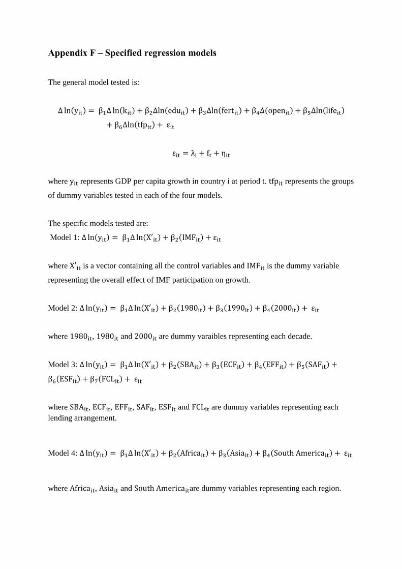
Appendix F – Specified regression models

The general model tested is:

( ( ( ( ( (

(

where represents GDP per capita growth in country i at period t. represents the groups

of dummy variables tested in each of the four models.

The specific models tested are:

Model 1: ( ( (

where is a vector containing all the control variables and is the dummy variable

representing the overall effect of IMF participation on growth.

Model 2: ( ( ( ( (

where , and are dummy varaibles representing each decade.

Model 3: ( ( ( ( ( (

( (

where , , , , and are dummy variables representing each

lending arrangement.

Model 4: ( ( ( ( (

where , and are dummy variables representing each region.