Embed Size (px)
Citation preview
The Imminent Practicality of Reversible Computing
Michael P. FrankUniversity of Florida
Departments of CISE and [email protected]
Talk at IBM ResearchYorktown Heights, New York
August 28, 2003
Arguably
Abstract• The practicality of reversible computing (RC), even for
the long-term, has historically been very controversial.– But, numerous deal-breakers conjectured for RC have already
succumbed to the steady march of engineering progress.
• The remaining few research-level engineering problems with RC do not appear to be fundamentally insoluble.– E.g., I discuss some simple design concepts for addressing the
leakage and power supply problems.
• A comprehensive numeric analysis forecasts orders-of-magnitude cost-efficiency benefits from RC growing over the next few decades, starting very soon!– I conclude with a technology R&D plan to achieve this goal.
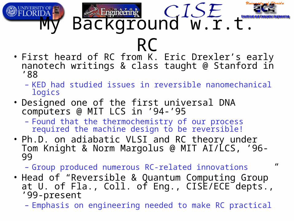
My Background w.r.t. RC• First heard of RC from K. Eric Drexler’s early
nanotech writings & class taught @ Stanford in ’88– KED had studied issues in reversible nanomechanical logics
• Designed one of the first universal DNA computers @ MIT LCS in ’94-’95– Found that the thermochemistry of our process required the
machine design to be reversible!• Ph.D. on adiabatic VLSI and RC theory under Tom
Knight & Norm Margolus @ MIT AI/LCS, ’96-99– Group produced numerous RC-related innovations
• Head of “Reversible & Quantum Computing Group” at U. of Fla., Coll. of Eng., CISE/ECE depts., ’99-present– Emphasis on engineering needed to make RC practical
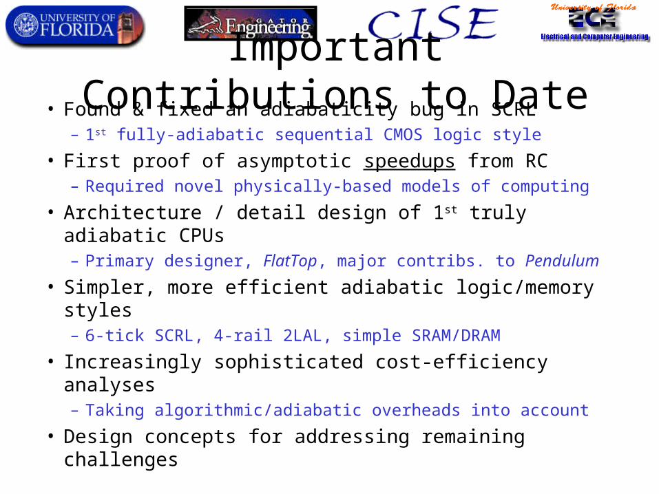
Important Contributions to Date• Found & fixed an adiabaticity bug in SCRL
– 1st fully-adiabatic sequential CMOS logic style
• First proof of asymptotic speedups from RC– Required novel physically-based models of computing
• Architecture / detail design of 1st truly adiabatic CPUs– Primary designer, FlatTop, major contribs. to Pendulum
• Simpler, more efficient adiabatic logic/memory styles– 6-tick SCRL, 4-rail 2LAL, simple SRAM/DRAM
• Increasingly sophisticated cost-efficiency analyses– Taking algorithmic/adiabatic overheads into account
• Design concepts for addressing remaining challenges
Moore’s Law vs. the Fundamental Physical Limits of Computing
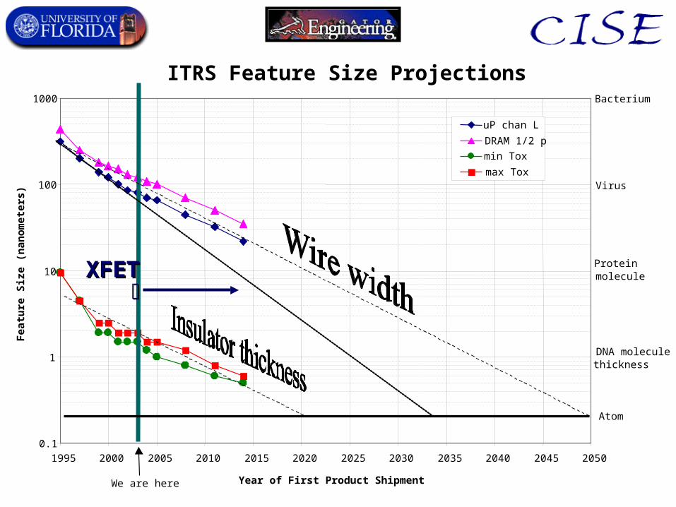
(From 1999 roadmap)
ITRS Feature Size Projections
0.1
1
10
100
1000
1995 2000 2005 2010 2015 2020 2025 2030 2035 2040 2045 2050
Year of First Product Shipment
Fea
ture
Siz
e (n
ano
met
ers)
uP chan L
DRAM 1/2 p
min Tox
max Tox
Atom
We are here
Virus
Proteinmolecule
DNA moleculethickness
Bacterium
XFETXFET
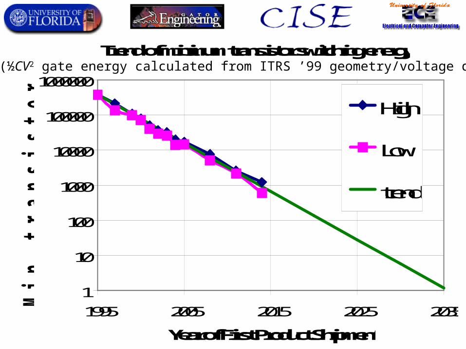
Trend of minimum transistor switching energy
1
10
100
1000
10000
100000
1000000
1995 2005 2015 2025 2035
Year of First Product Shipment
Min
tra
ns
isto
r s
wit
ch
ing
en
erg
y, kTs
High
Low
trend
(½CV2 gate energy calculated from ITRS ’99 geometry/voltage data)
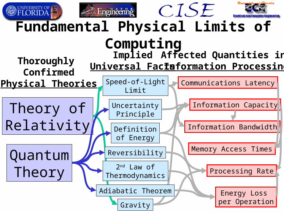
Fundamental Physical Limits of Computing
Speed-of-LightLimit
Thoroughly Confirmed
Physical Theories
UncertaintyPrinciple
Definitionof Energy
Reversibility
2nd Law ofThermodynamics
Adiabatic Theorem
Gravity
Theory ofRelativity
QuantumTheory
ImpliedUniversal Facts
Affected Quantities in Information Processing
Communications Latency
Information Capacity
Information Bandwidth
Memory Access Times
Processing Rate
Energy Loss per Operation
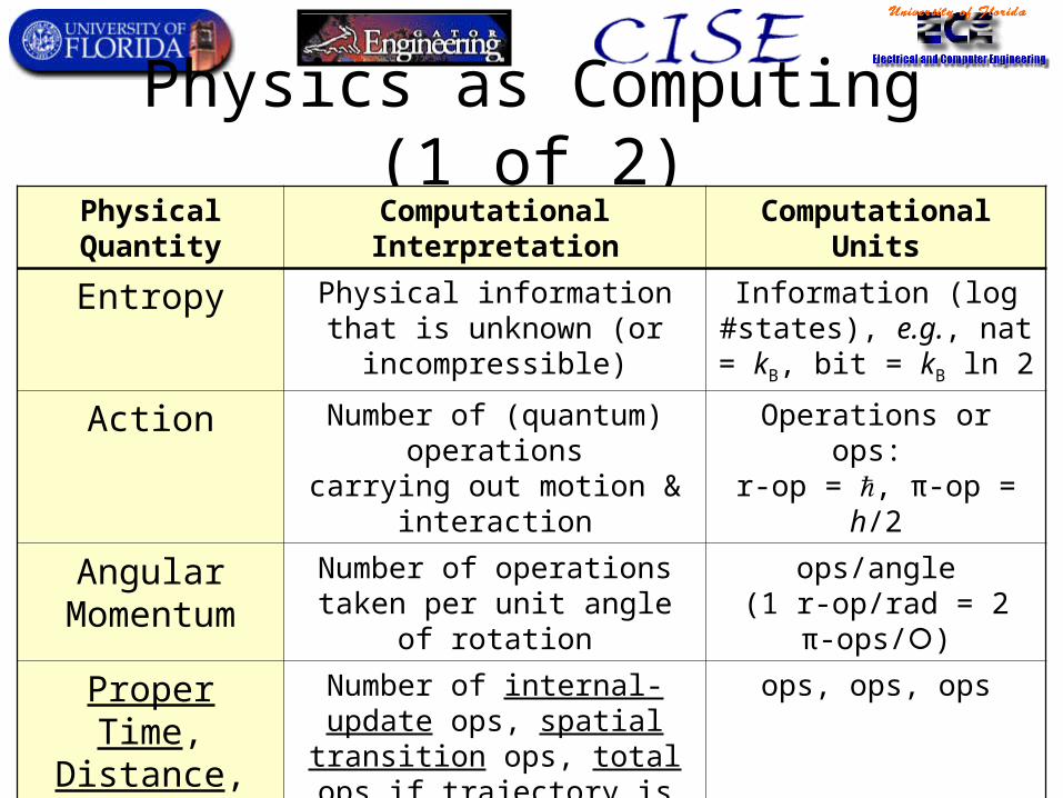
Physics as Computing (1 of 2)Physical Quantity Computational Interpretation Computational Units
Entropy Physical information that is unknown (or incompressible)
Information (log #states), e.g., nat = kB, bit = kB ln 2
Action Number of (quantum) operationscarrying out motion & interaction
Operations or ops: r-op = , π-op = h/2
Angular Momentum
Number of operations taken per unit angle of rotation
ops/angle(1 r-op/rad = 2 π-ops/)
Proper Time, Distance, Time
Number of internal-update ops, spatial transition ops, total ops if trajectory is taken by a reference system (Planck-mass particle?)
ops, ops, ops
Velocity2 Fraction of total ops of systemeffecting net spatial translation
ops/ops = dimensionless,max. value 100% (c2)
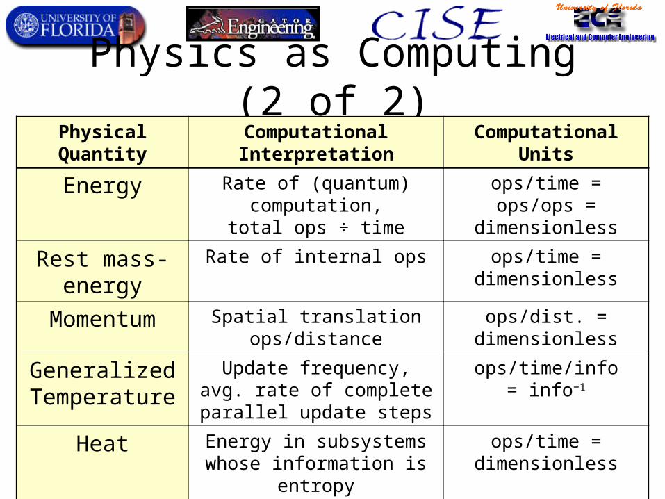
Physics as Computing (2 of 2)Physical Quantity Computational Interpretation Computational Units
Energy Rate of (quantum) computation,total ops ÷ time
ops/time = ops/ops = dimensionless
Rest mass-energy Rate of internal ops ops/time = dimensionless
Momentum Spatial translation ops/distance ops/dist. = dimensionless
GeneralizedTemperature
Update frequency, avg. rate of complete parallel update steps
ops/time/info= info−1
Heat Energy in subsystems whose information is entropy
ops/time = dimensionless
ThermalTemperature
Generalized temperature of subsystems whose information
is entropy
ops/time/info= info−1

Landauer’s 1961 principle from basic quantum theory
…Ndistinct
states
Ndistinct
states
……
2Ndistinctstates
Unitary(1-1)
evolution
Before bit erasure: After bit erasure:
Increase in entropy: S = log 2 = k ln 2. Energy lost to heat: ST = kT ln 2
0s0
0sN−1
…
1s′0
1s′N−1
…
…
0s″0
0s″N−1
0s″N
0s″2N−1
…
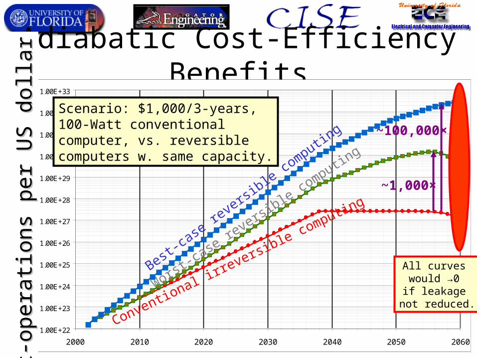
Adiabatic Cost-Efficiency Benefits
1.00E+22
1.00E+23
1.00E+24
1.00E+25
1.00E+26
1.00E+27
1.00E+28
1.00E+29
1.00E+30
1.00E+31
1.00E+32
1.00E+33
2000 2010 2020 2030 2040 2050 2060
Bit
-ope
rati
ons
per
US
dol
lar
Bit
-ope
rati
ons
per
US
dol
lar
Conventional irreversib
le computing
Worst-cas
e revers
ible computin
g
Best-ca
se rev
ersible
computin
g
Scenario: $1,000/3-years, 100-Watt conventional computer, vs. reversible computers w. same capacity.
All curves would →0 if leakage
not reduced.
~1,000×
~100,000×
Reversible Computing versus Quantum Computing
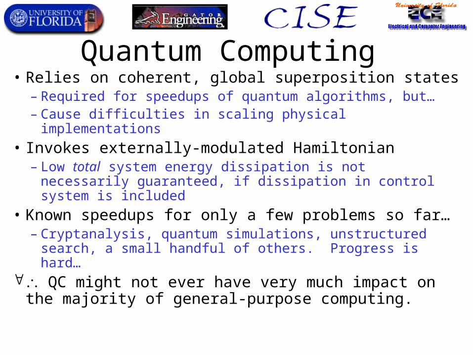
Quantum Computing • Relies on coherent, global superposition states
– Required for speedups of quantum algorithms, but… – Cause difficulties in scaling physical implementations
• Invokes externally-modulated Hamiltonian– Low total system energy dissipation is not necessarily
guaranteed, if dissipation in control system is included
• Known speedups for only a few problems so far…– Cryptanalysis, quantum simulations, unstructured
search, a small handful of others. Progress is hard… QC might not ever have very much impact on
the majority of general-purpose computing.
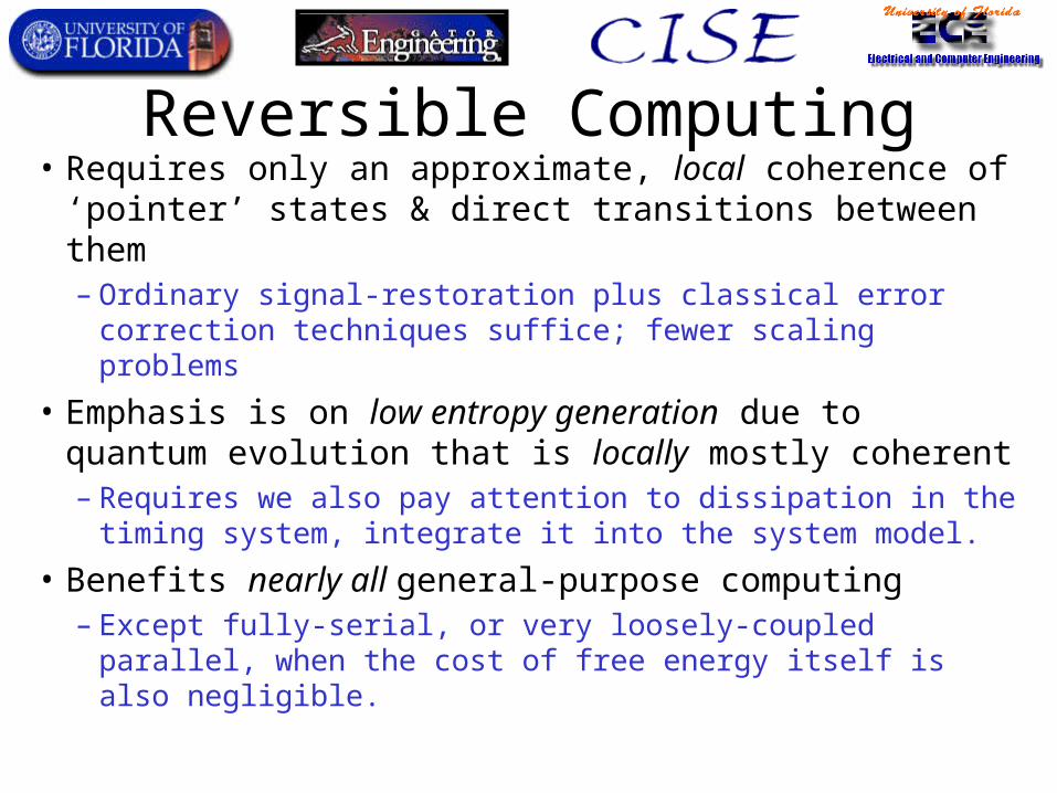
Reversible Computing• Requires only an approximate, local coherence of
‘pointer’ states & direct transitions between them– Ordinary signal-restoration plus classical error
correction techniques suffice; fewer scaling problems
• Emphasis is on low entropy generation due to quantum evolution that is locally mostly coherent– Requires we also pay attention to dissipation in the
timing system, integrate it into the system model.
• Benefits nearly all general-purpose computing– Except fully-serial, or very loosely-coupled parallel,
when the cost of free energy itself is also negligible.
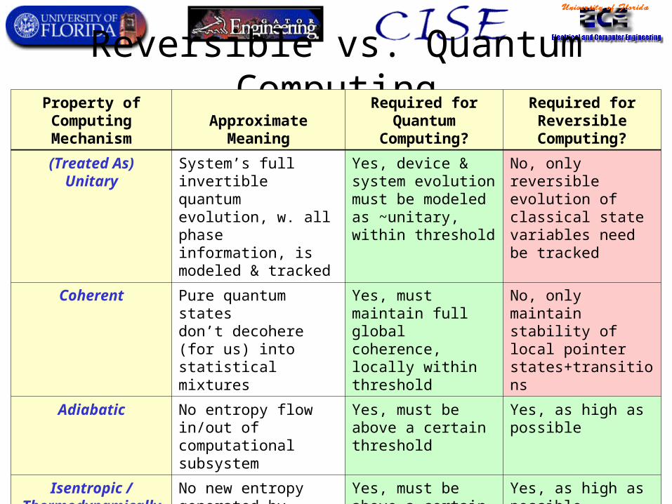
Reversible vs. Quantum ComputingProperty of Computing Mechanism Approximate Meaning
Required for Quantum Computing?
Required for Reversible
Computing?
(Treated As)Unitary
System’s full invertible quantum evolution, w. all phase information, is modeled & tracked
Yes, device & system evolution must be modeled as ~unitary, within threshold
No, only reversible evolution of classical state variables need be tracked
Coherent Pure quantum statesdon’t decohere (for us) into statistical mixtures
Yes, must maintain full global coherence, locally within threshold
No, only maintain stability of local pointer states+transitions
Adiabatic No entropy flow in/out of computational subsystem
Yes, must be above a certain threshold
Yes, as high as possible
Isentropic / Thermodynamically
Reversible
No new entropy generated by mechanism
Yes, must be above a certain threshold
Yes, as high as possible
Time-Independent Hamiltonian,
Self-Controlled
Closed system, evolves autonomously w/o external control
No, transitions can be externally timed & controlled
Yes, if we care about energy dissipation in the driving system
Ballistic System evolves w. net forward momentum
No, transitions can be externally driven
Yes, if we care about performance
The Fundamental Physical Limits of Computing

Fundamental Physical Limits of Computing
Speed-of-LightLimit
Thoroughly Confirmed
Physical Theories
UncertaintyPrinciple
Definitionof Energy
Reversibility
2nd Law ofThermodynamics
Adiabatic Theorem
Gravity
Theory ofRelativity
QuantumTheory
ImpliedUniversal Facts
Affected Quantities in Information Processing
Communications Latency
Information Capacity
Information Bandwidth
Memory Access Times
Processing Rate
Energy Loss per Operation
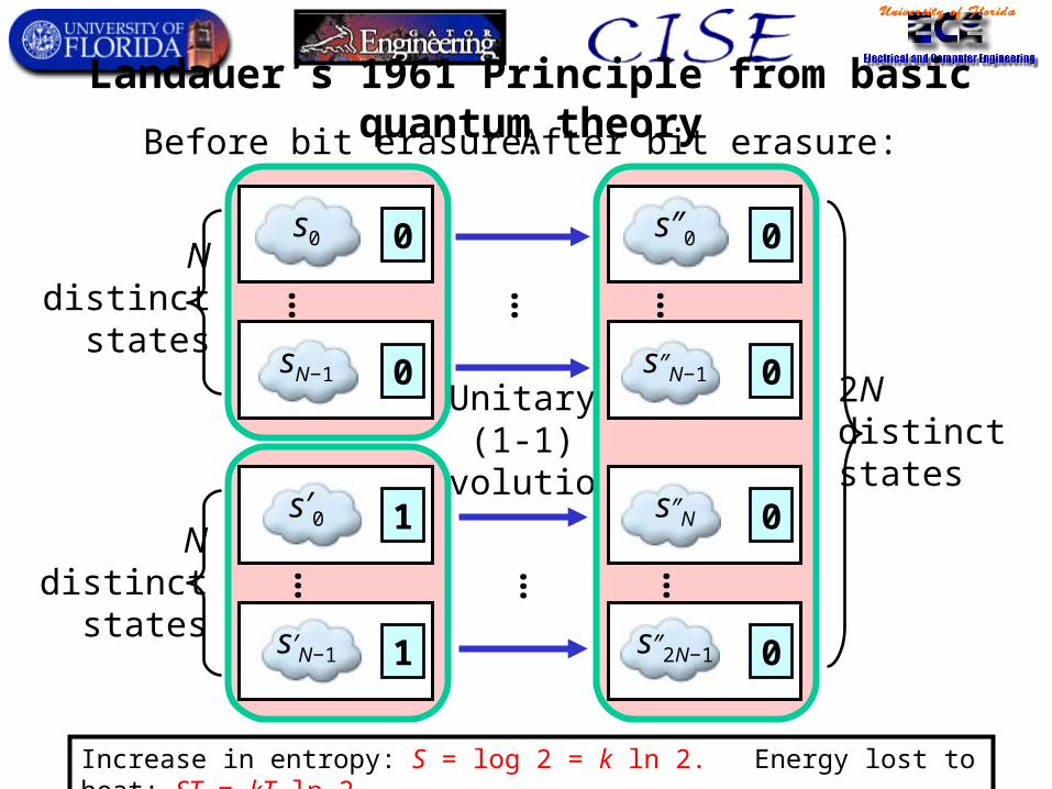
Landauer’s 1961 Principle from basic quantum theory
…Ndistinct
states
Ndistinct
states
……
2Ndistinctstates
Unitary(1-1)
evolution
Before bit erasure: After bit erasure:
Increase in entropy: S = log 2 = k ln 2. Energy lost to heat: ST = kT ln 2
0s0
0sN−1
…
1s′0
1s′N−1
…
…
0s″0
0s″N−1
0s″N
0s″2N−1
…
Reversible ComputingModels & Mechanisms
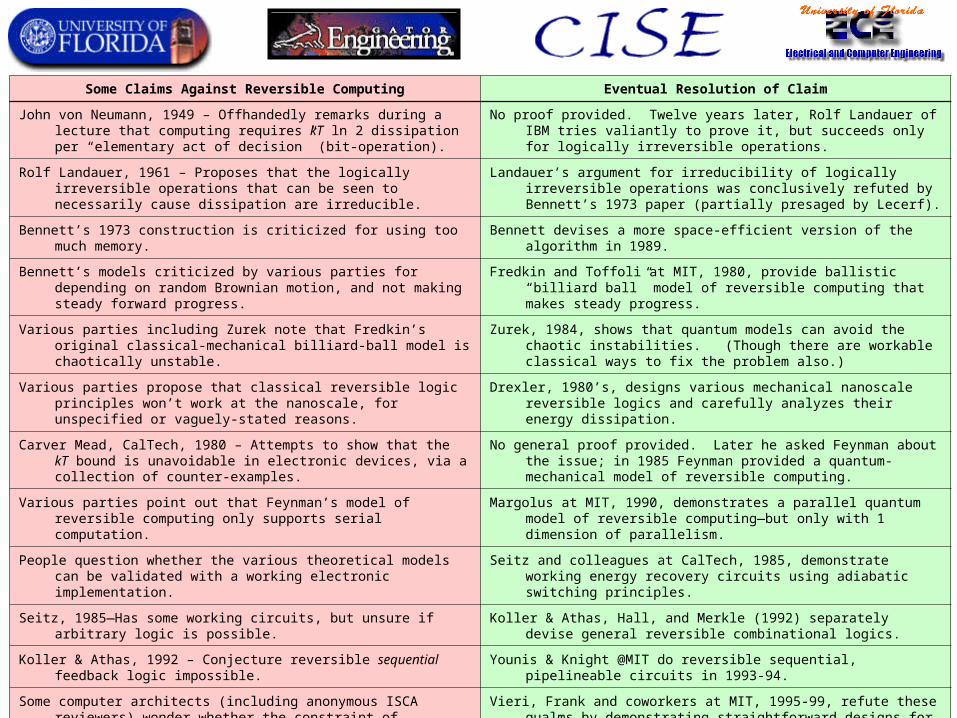
Some Claims Against Reversible Computing Eventual Resolution of Claim
John von Neumann, 1949 – Offhandedly remarks during a lecture that computing requires kT ln 2 dissipation per “elementary act of decision” (bit-operation).
No proof provided. Twelve years later, Rolf Landauer of IBM tries valiantly to prove it, but succeeds only for logically irreversible operations.
Rolf Landauer, 1961 – Proposes that the logically irreversible operations that can be seen to necessarily cause dissipation are irreducible.
Landauer’s argument for irreducibility of logically irreversible operations was conclusively refuted by Bennett’s 1973 paper (partially presaged by Lecerf).
Bennett’s 1973 construction is criticized for using too much memory. Bennett devises a more space-efficient version of the algorithm in 1989.
Bennett’s models criticized by various parties for depending on random Brownian motion, and not making steady forward progress.
Fredkin and Toffoli at MIT, 1980, provide ballistic “billiard ball” model of reversible computing that makes steady progress.
Various parties including Zurek note that Fredkin’s original classical-mechanical billiard-ball model is chaotically unstable.
Zurek, 1984, shows that quantum models can avoid the chaotic instabilities. (Though there are workable classical ways to fix the problem also.)
Various parties propose that classical reversible logic principles won’t work at the nanoscale, for unspecified or vaguely-stated reasons.
Drexler, 1980’s, designs various mechanical nanoscale reversible logics and carefully analyzes their energy dissipation.
Carver Mead, CalTech, 1980 – Attempts to show that the kT bound is unavoidable in electronic devices, via a collection of counter-examples.
No general proof provided. Later he asked Feynman about the issue; in 1985 Feynman provided a quantum-mechanical model of reversible computing.
Various parties point out that Feynman’s model of reversible computing only supports serial computation.
Margolus at MIT, 1990, demonstrates a parallel quantum model of reversible computing—but only with 1 dimension of parallelism.
People question whether the various theoretical models can be validated with a working electronic implementation.
Seitz and colleagues at CalTech, 1985, demonstrate working energy recovery circuits using adiabatic switching principles.
Seitz, 1985—Has some working circuits, but unsure if arbitrary logic is possible. Koller & Athas, Hall, and Merkle (1992) separately devise general reversible combinational logics.
Koller & Athas, 1992 – Conjecture reversible sequential feedback logic impossible. Younis & Knight @MIT do reversible sequential, pipelineable circuits in 1993-94.
Some computer architects (including anonymous ISCA reviewers) wonder whether the constraint of reversible logic leads to unreasonable design convolutions.
Vieri, Frank and coworkers at MIT, 1995-99, refute these qualms by demonstrating straightforward designs for fully-reversible and scalable gate arrays, microprocessors, and instruction sets.
Some computer science theorists suggest that the algorithmic overheads of reversible computing might outweigh their practical benefits.
Frank, 1997-2003, publishes a variety of rigorous theoretical analysis refuting these claims for the most general classes of applications.
Various parties point out that high-quality power supplies for adiabatic circuits seem difficult to build electronically.
Frank, 2000, suggests microscale/nanoscale electro mechanical resonators for high-quality energy recovery with desired waveform shape and frequency.
Frank, 2002—Briefly wonders if synchronization of parallel reversible computation in 3 dimensions (not covered by Margolus) might not be possible.
Later that year, Frank devises a simple mechanical model showing that parallel reversible systems can indeed be synchronized locally in 3 dimensions.
Focus of most of the work on adiabatics to date
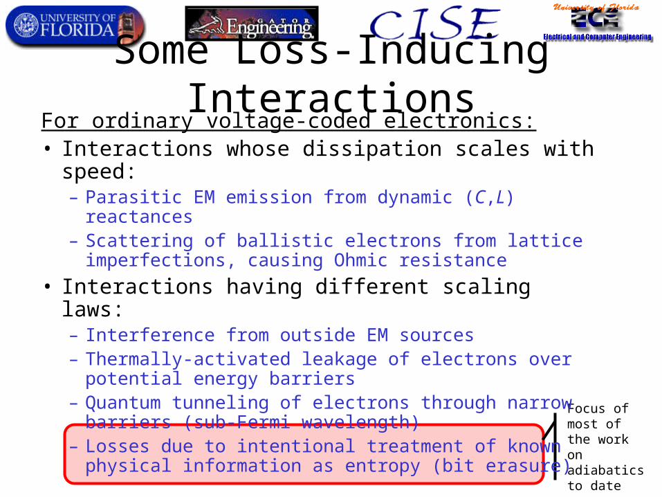
Some Loss-Inducing InteractionsFor ordinary voltage-coded electronics:• Interactions whose dissipation scales with speed:
– Parasitic EM emission from dynamic (C,L) reactances– Scattering of ballistic electrons from lattice
imperfections, causing Ohmic resistance
• Interactions having different scaling laws:– Interference from outside EM sources– Thermally-activated leakage of electrons over potential
energy barriers– Quantum tunneling of electrons through narrow barriers
(sub-Fermi wavelength)– Losses due to intentional treatment of known
physical information as entropy (bit erasure)
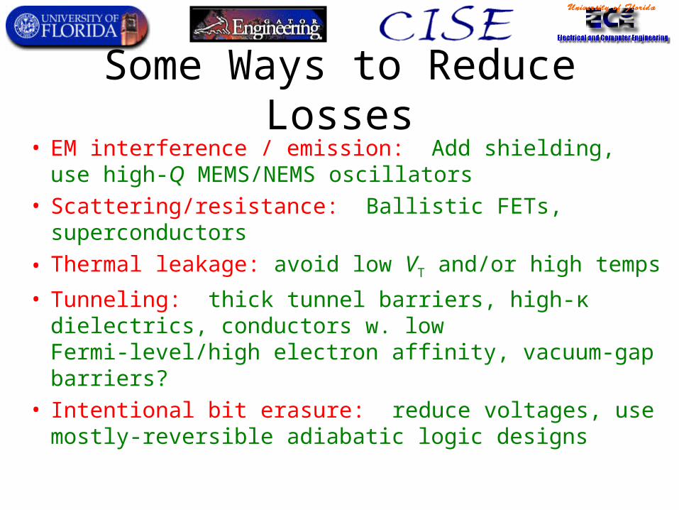
Some Ways to Reduce Losses• EM interference / emission: Add shielding, use high-Q
MEMS/NEMS oscillators• Scattering/resistance: Ballistic FETs, superconductors
• Thermal leakage: avoid low VT and/or high temps
• Tunneling: thick tunnel barriers, high-κ dielectrics, conductors w. low Fermi-level/high electron affinity, vacuum-gap barriers?
• Intentional bit erasure: reduce voltages, use mostly-reversible adiabatic logic designs
Adiabatic Circuits and Reversible Computing
Commonly Encountered Myths, Fallacies, and Pitfalls
(in the Hennessy-Patterson tradition)
Myths about Adiabatic Circuits & Reversible Computing
• “Someone proved that computing with <<kT free-energy loss per bit-operation is impossible.”
• “Physics isn’t reversible.”
• “An energy-efficient adiabatic clock/power supply is impossible to build.”
• “True adiabaticity doesn’t require reversible logic.”
• “Sequential logic can’t be done adiabatically.”
• “Adiabatic circuits require many clock/power rails and/or voltage levels.”
• “Adiabatic design is necessarily difficult.”
Fallacies about Adiabatic Circuits and Reversible Computing
• “Since speed scales with energy dissipation in adiabatic circuits, they aren’t good for high-performance computing.”
• “If I tried and failed to invent an efficient adiabatic logic, it must be impossible.”
• “The algorithmic overheads of reversible computing mean it can never be cost-effective.”
• “Since leakage gets worse in nanoscale devices, adiabatics is doomed.”
Pitfalls in Adiabatic Circuits and Reversible Computing
• Using diodes in the charge-return path.
• Forgetting to obey one of the transistor rules.
• Using traditional models of computational complexity.
• Restricting oneself to an asymptotically inefficient design style.
• Assuming that the best reversible and irreversible algorithms are similar.
• Failing to optimize the degree of reversibility of a design.
• Ignoring charge leakage in low-power/adiabatic design.
Adiabatic/Reversible Computing
Basic Models and Concepts
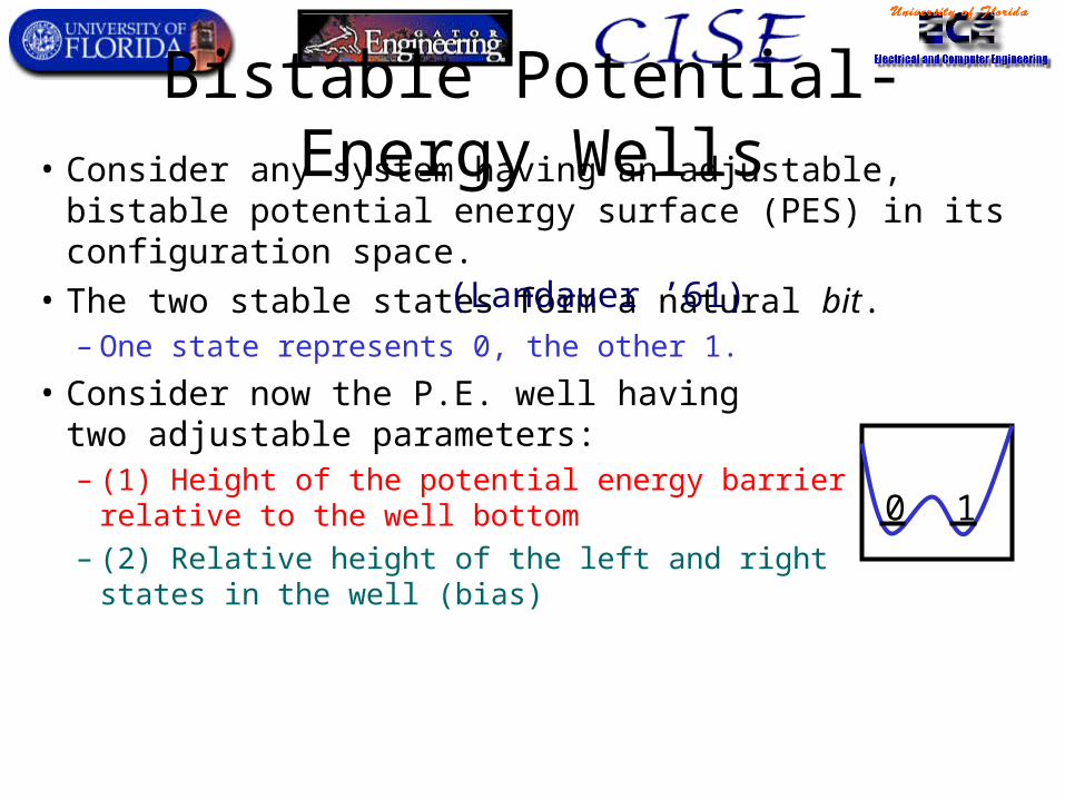
Bistable Potential-Energy Wells• Consider any system having an adjustable, bistable potential
energy surface (PES) in its configuration space.
• The two stable states form a natural bit.– One state represents 0, the other 1.
• Consider now the P.E. well havingtwo adjustable parameters:– (1) Height of the potential energy barrier
relative to the well bottom– (2) Relative height of the left and right
states in the well (bias)
0 1
(Landauer ’61)
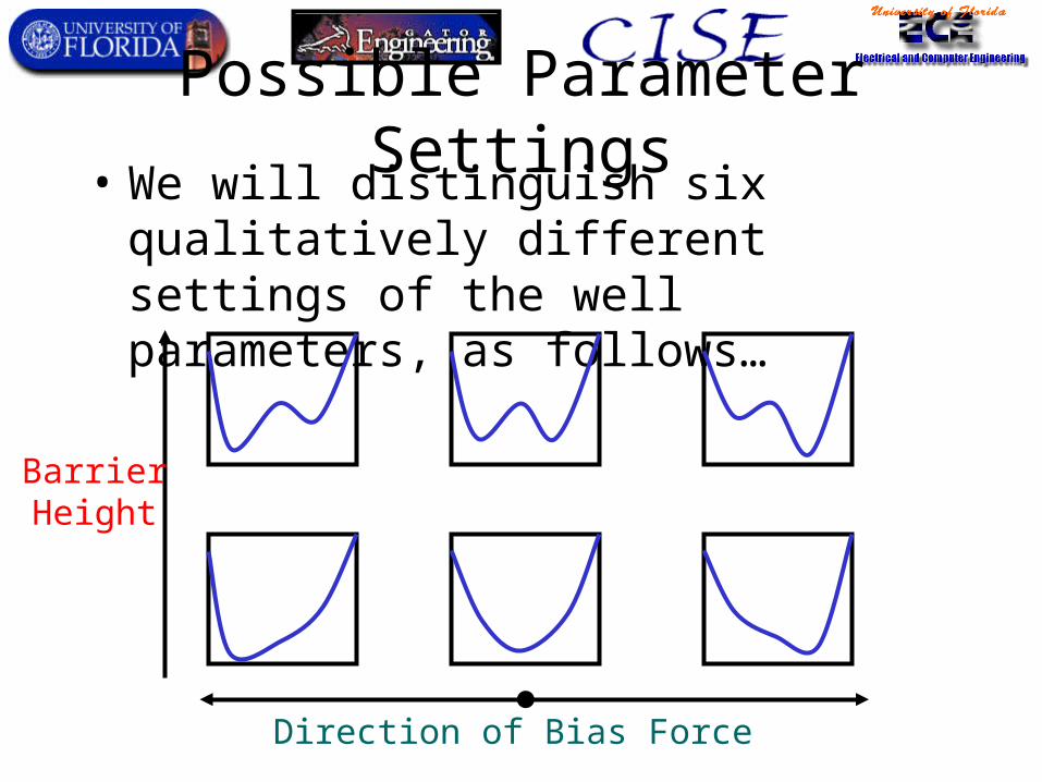
Possible Parameter Settings• We will distinguish six qualitatively
different settings of the well parameters, as follows…
Direction of Bias Force
BarrierHeight
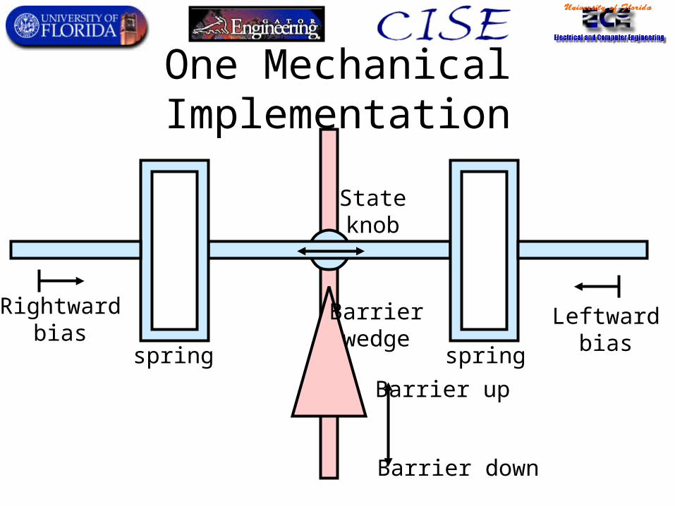
One Mechanical Implementation
spring spring
Rightwardbias
Leftwardbias
Barrier up
Barrier down
Barrierwedge
Stateknob
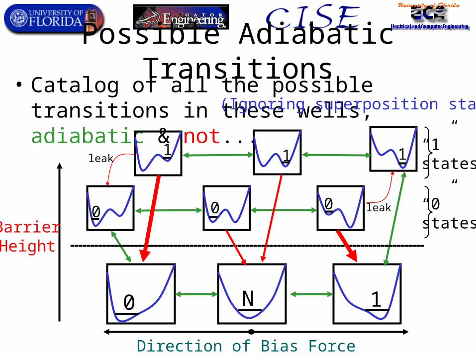
Possible Adiabatic Transitions• Catalog of all the possible transitions in
these wells, adiabatic & not...
Direction of Bias Force
BarrierHeight
0 0 0
111
10 N
(Ignoring superposition states.)
leak
leak
“1”states
“0”states
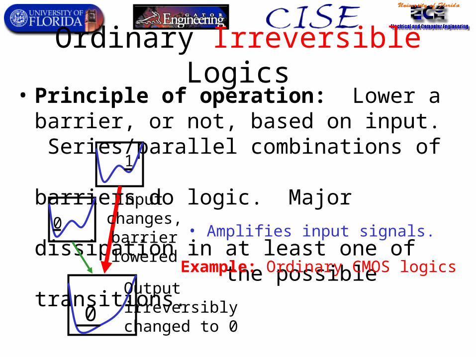
Ordinary Irreversible Logics• Principle of operation: Lower a barrier, or not,
based on input. Series/parallel combinations of barriers do logic. Major dissipation in at least one of
the possible transitions.0
1
0
Example: Ordinary CMOS logics
Input changes,barrier
lowered
Outputirreversiblychanged to 0
• Amplifies input signals.
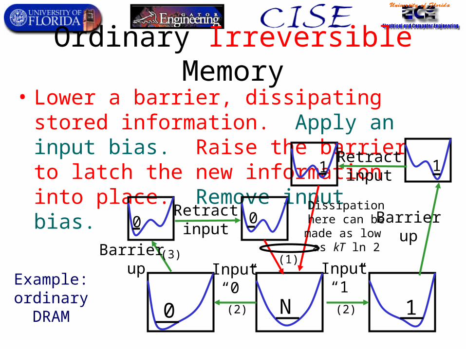
Ordinary Irreversible Memory
• Lower a barrier, dissipating stored information. Apply an input bias. Raise the barrier to latch the new informationinto place. Remove inputbias.
0 0
11
10 N
Example:ordinaryDRAM
Dissipationhere can be
made as low as kT ln 2
Input“0”
Input“1”
Barrier up
Barrierup
Retractinput
Retractinput
(1)
(2) (2)
(3)
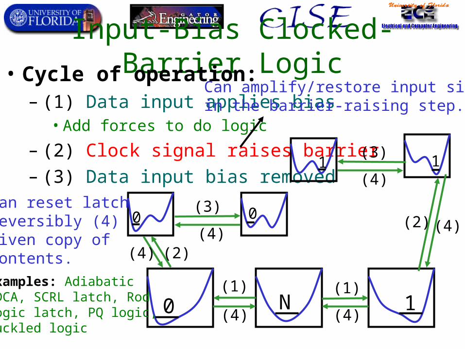
Input-Bias Clocked-Barrier Logic• Cycle of operation:
– (1) Data input applies bias• Add forces to do logic
– (2) Clock signal raises barrier– (3) Data input bias removed
0 0
11
10 N
Can amplify/restore input signalin the barrier-raising step.
Can reset latch reversibly (4) given copy ofcontents.
Examples: AdiabaticQDCA, SCRL latch, Rod logic latch, PQ logic,Buckled logic
(1) (1)
(2)
(2)(3)
(3)
(4)(4)
(4) (4)
(4)
(4)
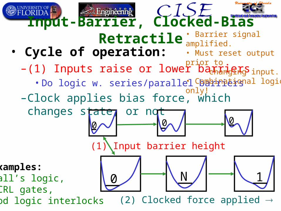
Input-Barrier, Clocked-Bias Retractile
• Cycle of operation:– (1) Inputs raise or lower barriers
• Do logic w. series/parallel barriers
– Clock applies bias force, which changes state, or not
0 0 0
10 N
• Barrier signal amplified.• Must reset output prior to changing input.• Combinational logic only!
(1) Input barrier height
(2) Clocked force applied
Examples:Hall’s logic,SCRL gates,Rod logic interlocks
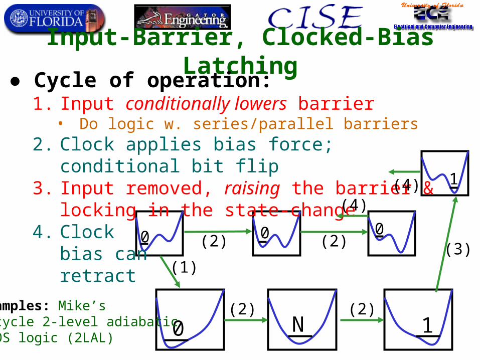
Input-Barrier, Clocked-Bias Latching
0 0 0
1
10 N
● Cycle of operation:1. Input conditionally lowers barrier
• Do logic w. series/parallel barriers2. Clock applies bias force; conditional bit flip3. Input removed, raising the barrier &
locking in the state-change4. Clock
bias canretract
Examples: Mike’s4-cycle 2-level adiabaticCMOS logic (2LAL)
(1)
(2) (2)
(2) (2)
(3)
(4)(4)
Sleeve
(a)
(b)
(c)
(d)
(e)
(f)
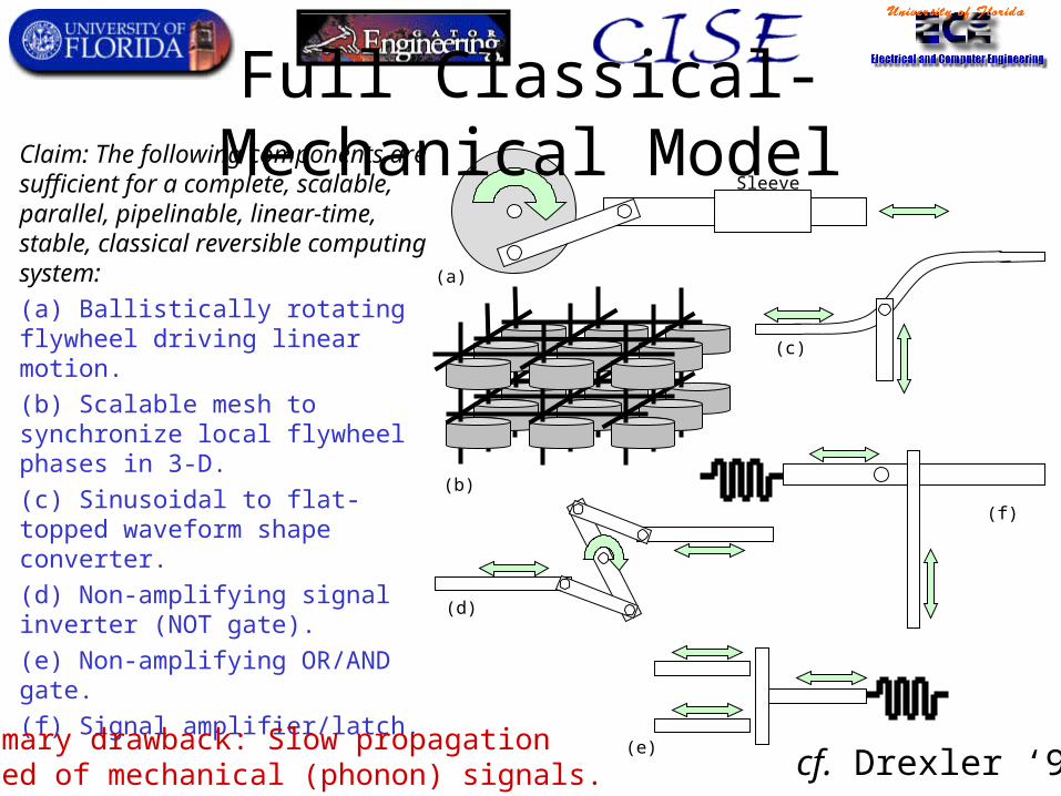
Full Classical-Mechanical ModelClaim: The following components are sufficient for a complete, scalable, parallel, pipelinable, linear-time, stable, classical reversible computing system:
(a) Ballistically rotating flywheel driving linear motion.
(b) Scalable mesh to synchronize local flywheel phases in 3-D.
(c) Sinusoidal to flat-topped waveform shape converter.
(d) Non-amplifying signal inverter (NOT gate).
(e) Non-amplifying OR/AND gate.
(f) Signal amplifier/latch.
Primary drawback: Slow propagationspeed of mechanical (phonon) signals. cf. Drexler ‘92
Common Mistakes to Avoid
In Adiabatic Design
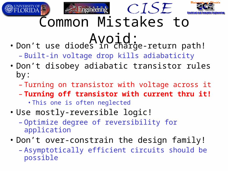
Common Mistakes to Avoid:• Don’t use diodes in charge-return path!
– Built-in voltage drop kills adiabaticity
• Don’t disobey adiabatic transistor rules by:– Turning on transistor with voltage across it– Turning off transistor with current thru it!
• This one is often neglected
• Use mostly-reversible logic!– Optimize degree of reversibility for application
• Don’t over-constrain the design family!– Asymptotically efficient circuits should be possible
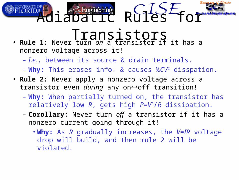
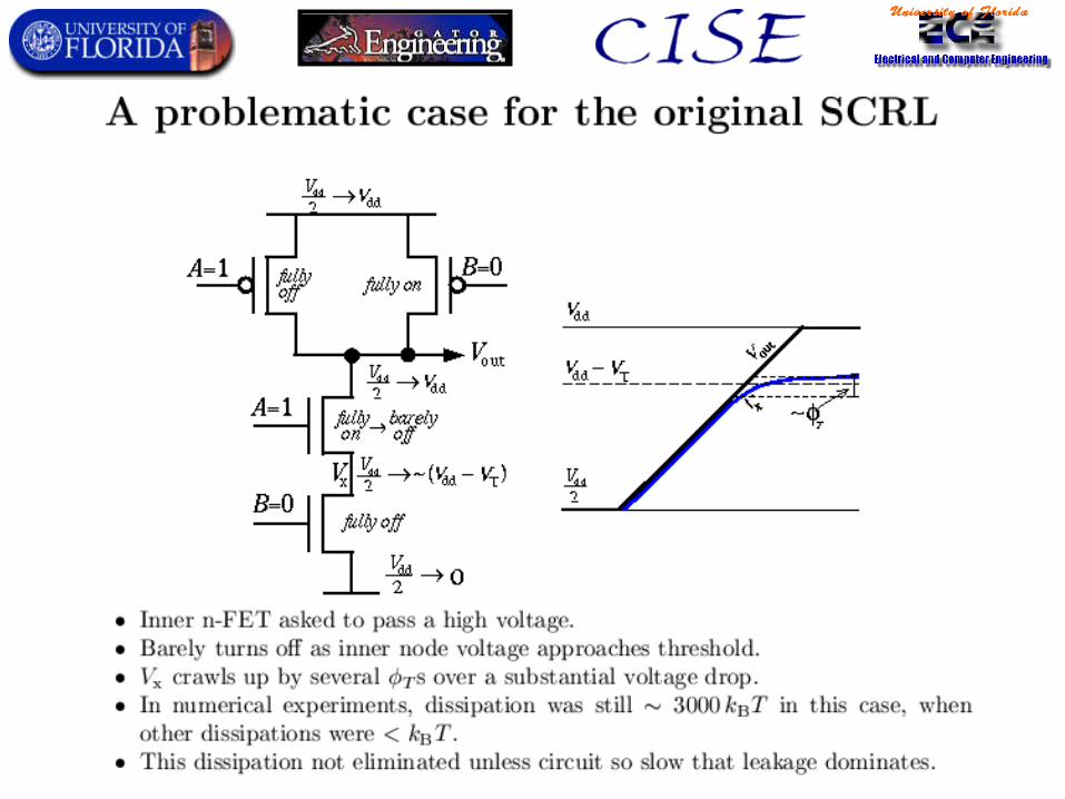
Adiabatic Rules for Transistors• Rule 1: Never turn on a transistor if it has a nonzero voltage
across it!– I.e., between its source & drain terminals.– Why: This erases info. & causes ½CV2 disspation.
• Rule 2: Never apply a nonzero voltage across a transistor even during any onoff transition!– Why: When partially turned on, the transistor has relatively
low R, gets high P=V2/R dissipation.– Corollary: Never turn off a transistor if it has a nonzero
current going through it!• Why: As R gradually increases, the V=IR voltage drop will
build, and then rule 2 will be violated.
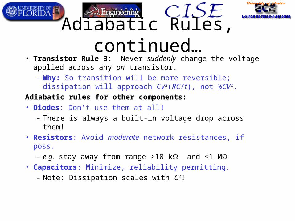
Adiabatic Rules, continued…• Transistor Rule 3: Never suddenly change the voltage applied
across any on transistor.
– Why: So transition will be more reversible; dissipation will approach CV2(RC/t), not ½CV2.
Adiabatic rules for other components:
• Diodes: Don’t use them at all!
– There is always a built-in voltage drop across them!
• Resistors: Avoid moderate network resistances, if poss.
– e.g. stay away from range >10 k and <1 M• Capacitors: Minimize, reliability permitting.
– Note: Dissipation scales with C2!
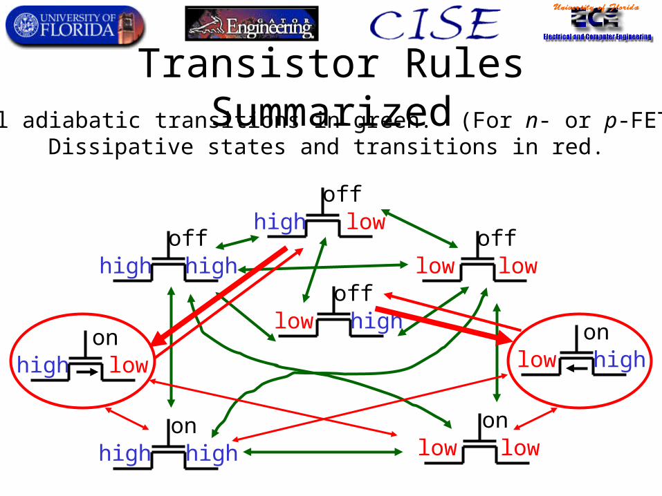
Transistor Rules Summarized
offhigh high
onhigh low
offhigh
offlow low
low
onhigh high
onlow low
Legal adiabatic transitions in green. (For n- or p-FETs.)Dissipative states and transitions in red.
offhigh low
onhighlow
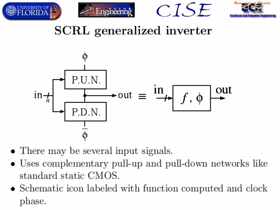
SCRL: Split-level Charge Recovery Logic
The First Pipelined Fully-Adiabatic CMOS Logic
(Younis & Knight, MIT, ’94)
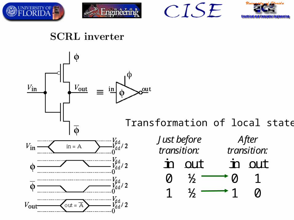
Just beforetransition:
Aftertransition:
in out in out0 ½ 0 11 ½ 1 0
Transformation of local state:
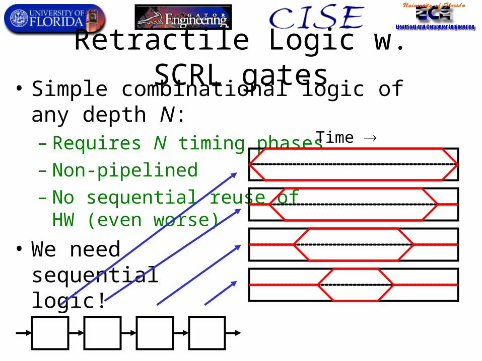
Retractile Logic w. SCRL gates• Simple combinational logic of any depth N:
– Requires N timing phases– Non-pipelined– No sequential reuse of
HW (even worse)
• We needsequentiallogic!
Time
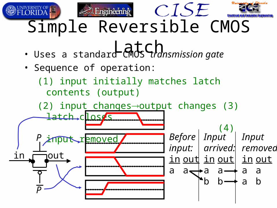
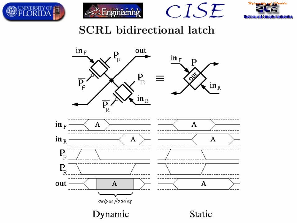
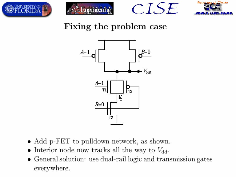
Simple Reversible CMOS Latch• Uses a standard CMOS transmission gate
• Sequence of operation:
(1) input initially matches latch contents (output)
(2) input changesoutput changes (3) latch closes (4) input
removed
P
P
in out
Before Input Inputinput: arrived: removed:in out in out in outa a a a a a
b b a b
Resetting a Reversible Latch
• Can reversibly unlatch data as follows: (exactly the reverse of the latching process)– (1) Data value d stored on memory node M.– (2) Present an exact copy of d on input.– (3) Open the latch (connecting input to M).
• No dissipation since voltage levels match
– (4) Retract the copy of d from the input.• Retracts copy stored in latch also.
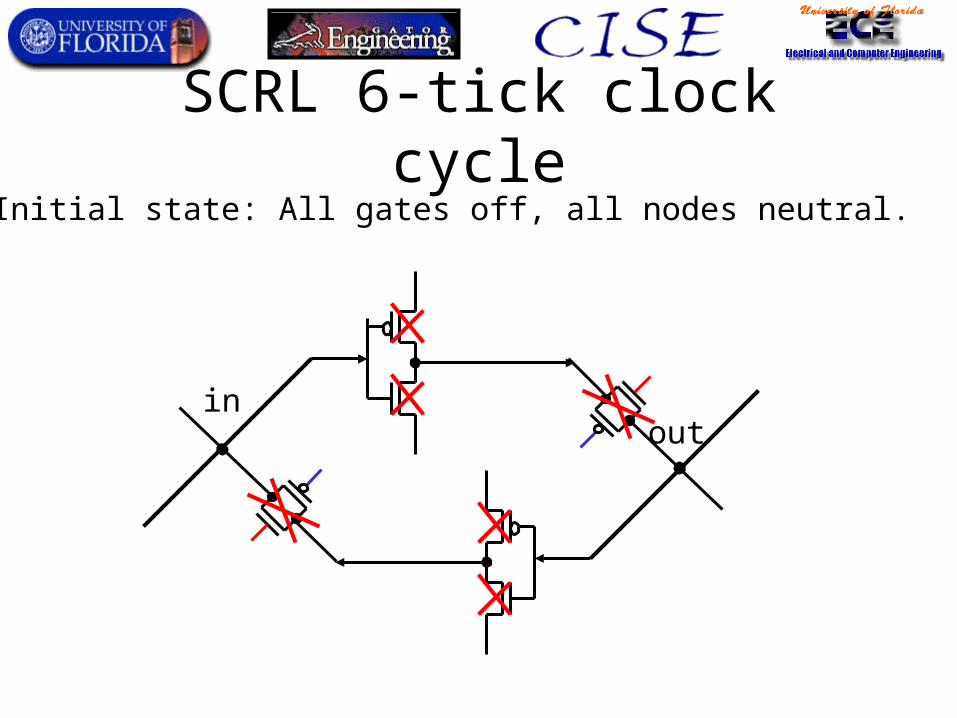
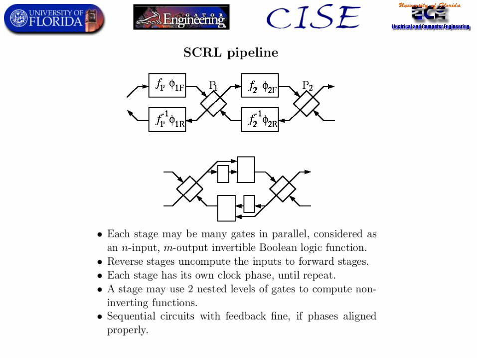
SCRL 6-tick clock cycle
inout
Initial state: All gates off, all nodes neutral.
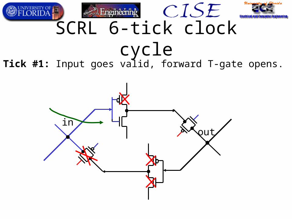
SCRL 6-tick clock cycle
inout
Tick #1: Input goes valid, forward T-gate opens.
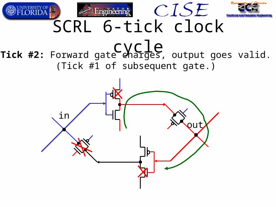
SCRL 6-tick clock cycle
inout
Tick #2: Forward gate charges, output goes valid.(Tick #1 of subsequent gate.)
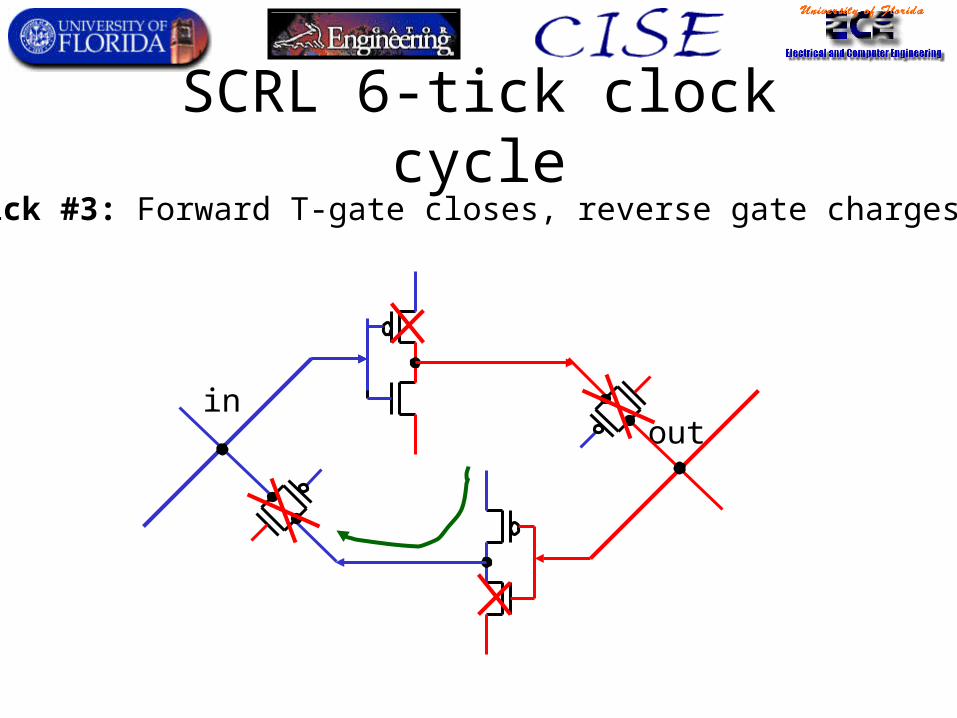
SCRL 6-tick clock cycle
inout
Tick #3: Forward T-gate closes, reverse gate charges.
SCRL 6-tick clock cycle
inout
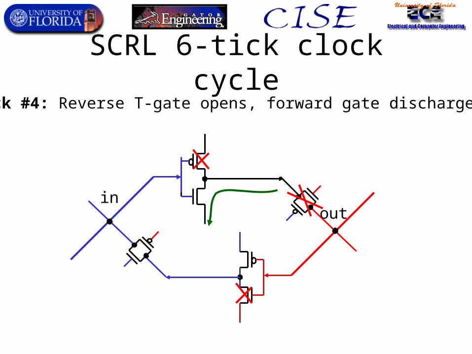
Tick #4: Reverse T-gate opens, forward gate discharges.
SCRL 6-tick clock cycle
inout
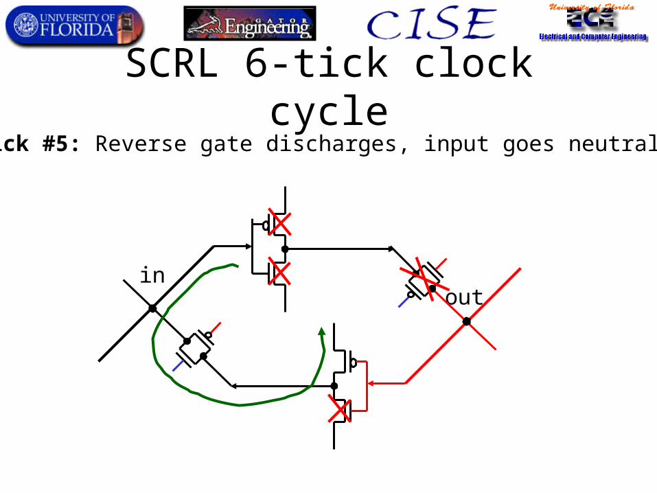
Tick #5: Reverse gate discharges, input goes neutral.
SCRL 6-tick clock cycle
inout
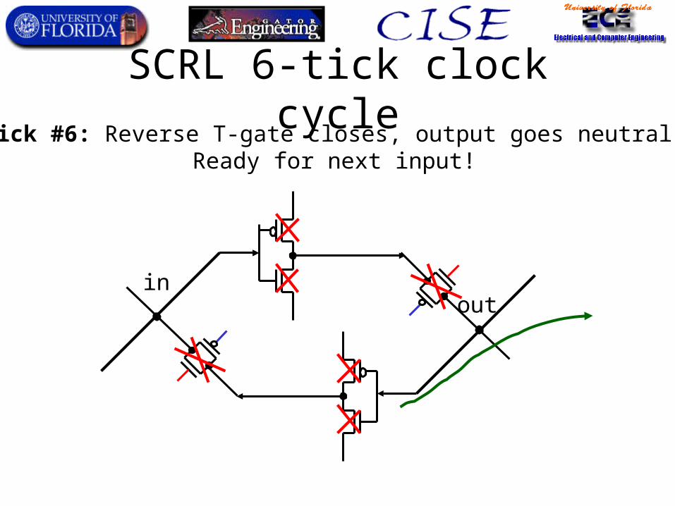
Tick #6: Reverse T-gate closes, output goes neutral.Ready for next input!
2LAL: 2-Level Adiabatic Logic
A Novel Alternative to SCRL
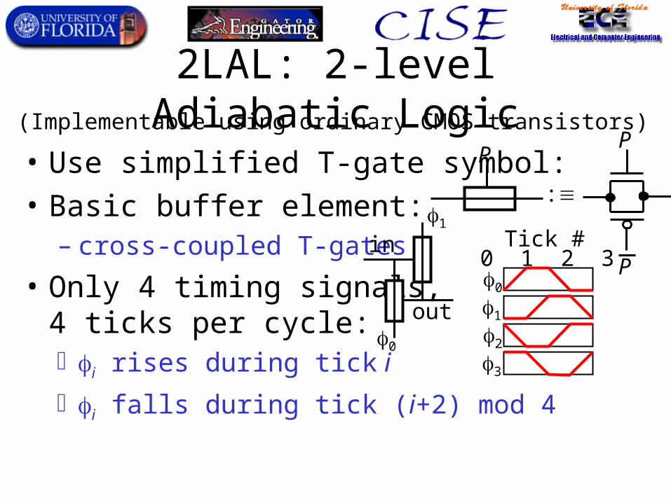
2LAL: 2-level Adiabatic Logic
• Use simplified T-gate symbol:
• Basic buffer element:– cross-coupled T-gates
• Only 4 timing signals,4 ticks per cycle: i rises during tick i
i falls during tick (i+2) mod 4
P
P
P
:
in
out
1
0
0 1 2 3Tick #
0
1
2
3
(Implementable using ordinary CMOS transistors)
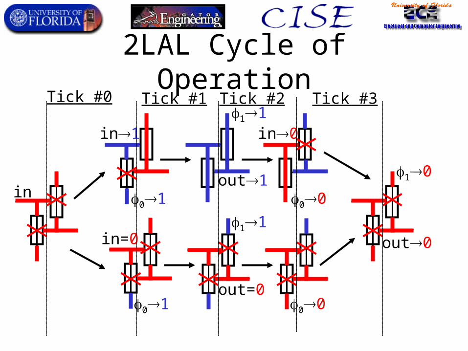
2LAL Cycle of Operation
in
in1
in=0
01
01
10
11
out1
out=0
00
00
in011
out0
Tick #0 Tick #1 Tick #2 Tick #3
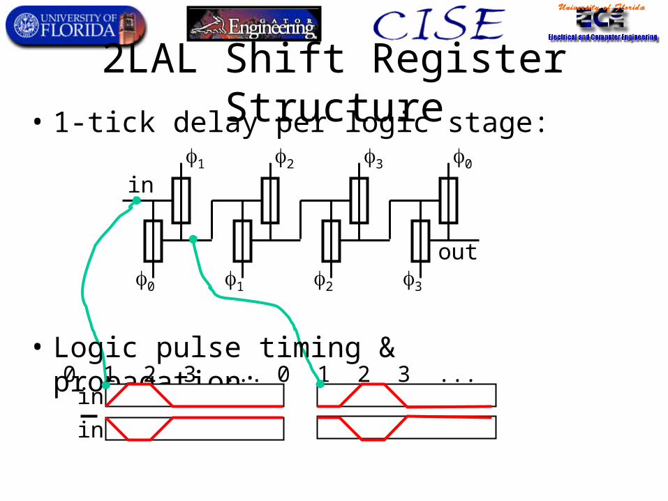
2LAL Shift Register Structure• 1-tick delay per logic stage:
• Logic pulse timing & propagation:
in1
0
2
1
3
2
out
0
3
in
in
0 1 2 3 ... 0 1 2 3 ...
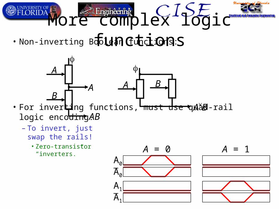
More complex logic functions• Non-inverting Boolean functions:
• For inverting functions, must use quad-rail logic encoding:– To invert, just
swap the rails!• Zero-transistor
“inverters.”
A
B
A
AB
A B
AB
A0
A0
A1
A1
A = 0 A = 1
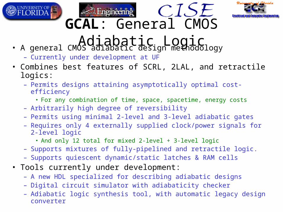
GCAL: General CMOS Adiabatic Logic• A general CMOS adiabatic design methodology
– Currently under development at UF
• Combines best features of SCRL, 2LAL, and retractile logics:– Permits designs attaining asymptotically optimal cost-efficiency
• For any combination of time, space, spacetime, energy costs
– Arbitrarily high degree of reversibility– Permits using minimal 2-level and 3-level adiabatic gates– Requires only 4 externally supplied clock/power signals for 2-level logic
• And only 12 total for mixed 2-level + 3-level logic
– Supports mixtures of fully-pipelined and retractile logic.– Supports quiescent dynamic/static latches & RAM cells
• Tools currently under development:– A new HDL specialized for describing adiabatic designs– Digital circuit simulator with adiabaticity checker– Adiabatic logic synthesis tool, with automatic legacy design converter
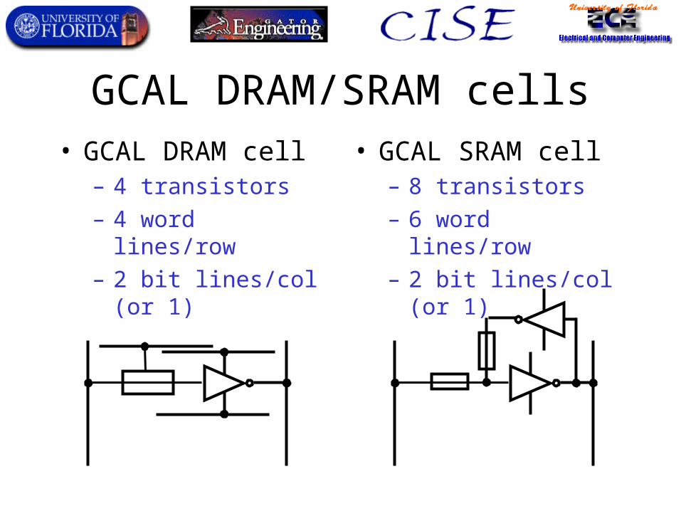
GCAL DRAM/SRAM cells• GCAL DRAM cell
– 4 transistors
– 4 word lines/row
– 2 bit lines/col (or 1)
• GCAL SRAM cell– 8 transistors
– 6 word lines/row
– 2 bit lines/col (or 1)
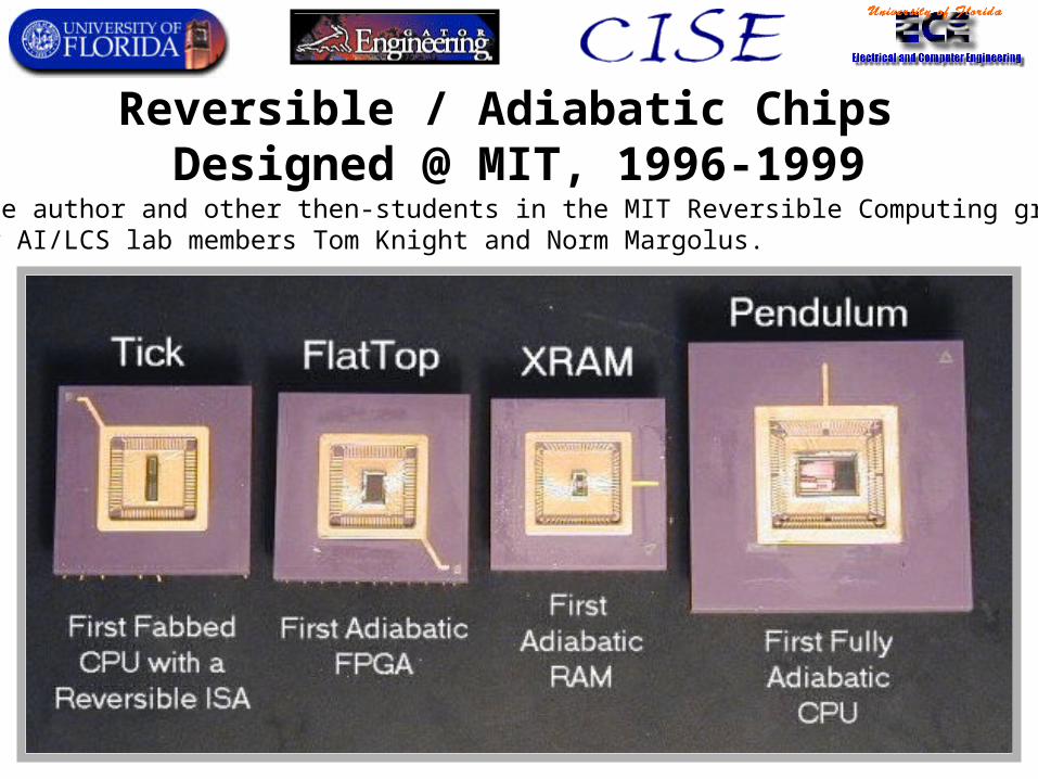
Reversible / Adiabatic Chips Designed @ MIT, 1996-1999
By the author and other then-students in the MIT Reversible Computing group,under AI/LCS lab members Tom Knight and Norm Margolus.
MEMS/NEMS Resonators
A Novel Clock/Power Supply Technology for Adiabatic Circuits
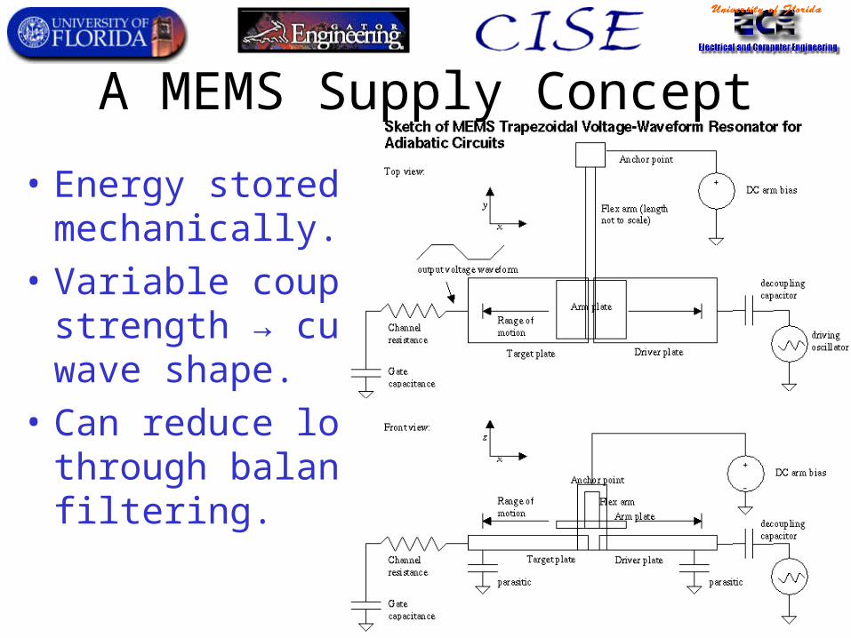
• Energy storedmechanically.
• Variable couplingstrength → customwave shape.
• Can reduce lossesthrough balancing,filtering.
A MEMS Supply Concept
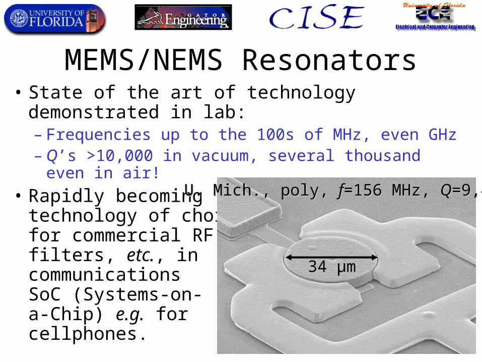
MEMS/NEMS Resonators• State of the art of technology demonstrated in
lab:– Frequencies up to the 100s of MHz, even GHz– Q’s >10,000 in vacuum, several thousand even in air!
• Rapidly becoming technology of choicefor commercial RF filters, etc., in communicationsSoC (Systems-on-a-Chip) e.g. for cellphones.
U. Mich., poly, U. Mich., poly, ff=156 MHz, =156 MHz, QQ=9,400=9,400
34 µm
Nanocomputer Systems Engineering
Analyzing & Optimizing the Benefits of Reversible Computing
• Claim: All practical engineering design-optimization can ultimately be reduced to maximization of a generalized, system-level measure of cost-efficiency.– Given appropriate models of cost “$”.
• Definition of the Cost-Efficiency %$ of a process: %$ :≡ $min/$actual
• Maximize %$ by minimizing $actual
– Note this is valid even when $min is unknown
Cost-Efficiency:The Key Figure of Merit
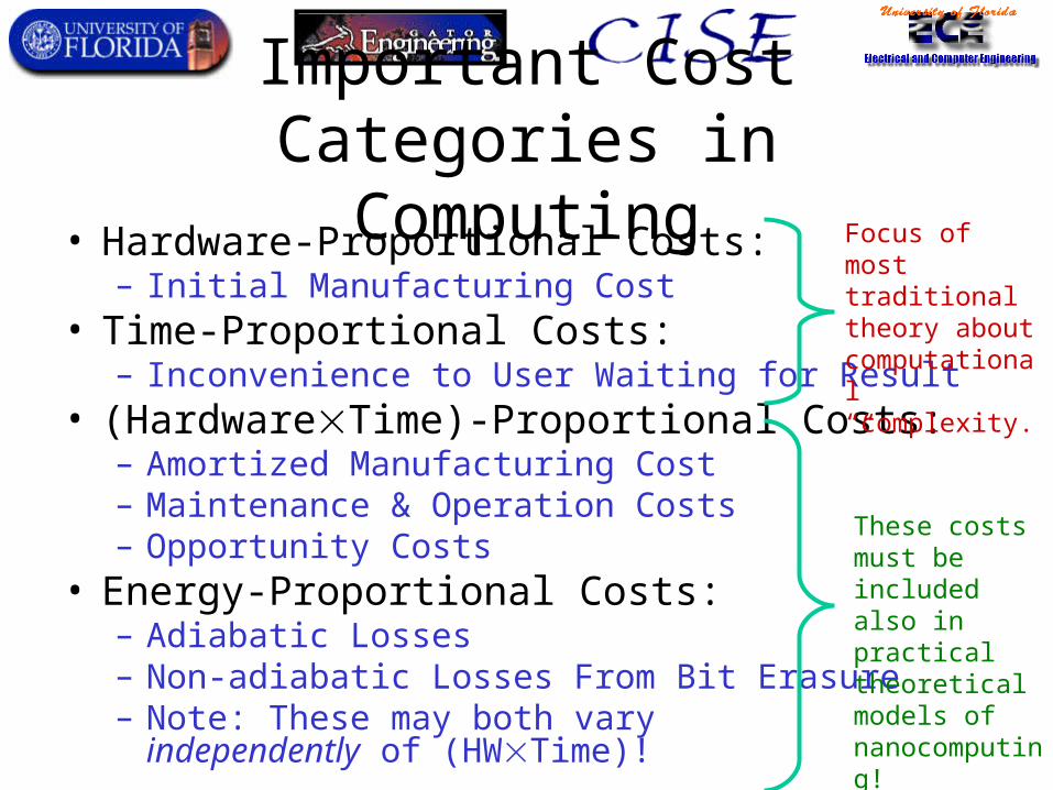
Important Cost Categories in Computing
• Hardware-Proportional Costs:– Initial Manufacturing Cost
• Time-Proportional Costs:– Inconvenience to User Waiting for Result
• (HardwareTime)-Proportional Costs:– Amortized Manufacturing Cost– Maintenance & Operation Costs– Opportunity Costs
• Energy-Proportional Costs:– Adiabatic Losses– Non-adiabatic Losses From Bit Erasure– Note: These may both vary
independently of (HWTime)!
Focus of mosttraditionaltheory aboutcomputational“complexity.”
These costsmust be included also in practicaltheoreticalmodels ofnanocomputing!
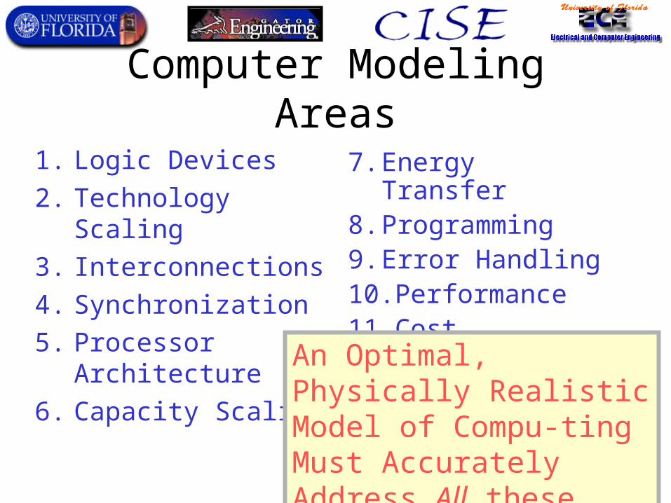
Computer Modeling Areas
1. Logic Devices
2. Technology Scaling
3. Interconnections
4. Synchronization
5. Processor Architecture
6. Capacity Scaling
7. Energy Transfer8. Programming9. Error Handling10.Performance11.Cost
An Optimal, Physically Realistic Model of Compu-ting Must Accurately Address All these Areas!
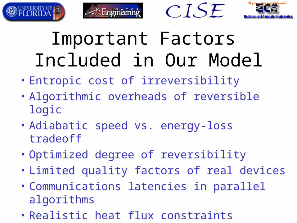
Important Factors Included in Our Model
• Entropic cost of irreversibility
• Algorithmic overheads of reversible logic
• Adiabatic speed vs. energy-loss tradeoff
• Optimized degree of reversibility
• Limited quality factors of real devices
• Communications latencies in parallel algorithms
• Realistic heat flux constraints
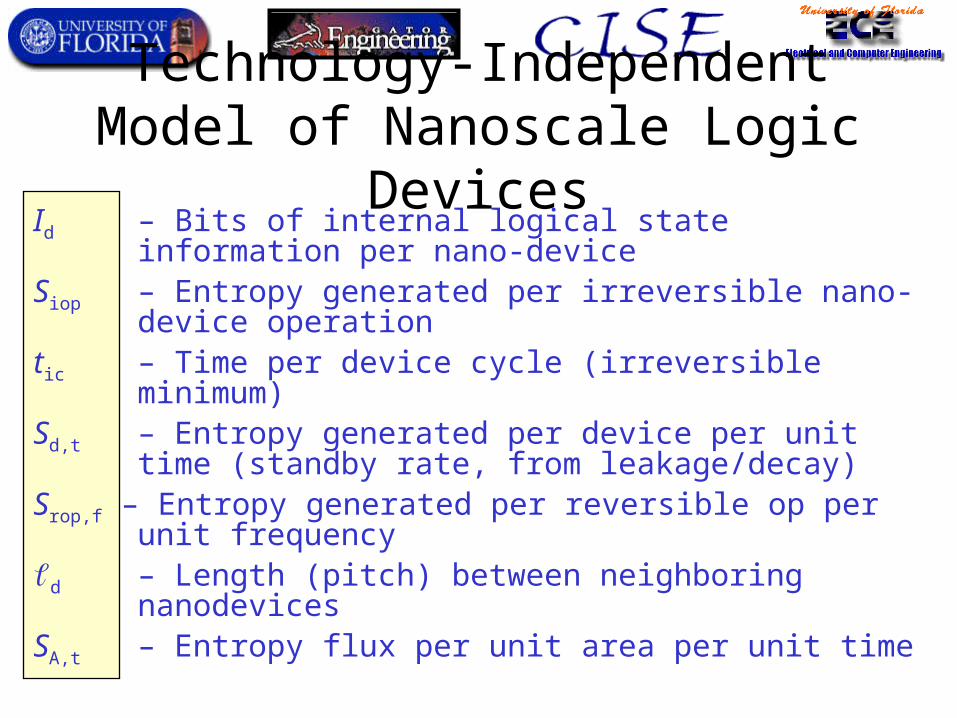
Technology-Independent Model of Nanoscale Logic Devices
Id – Bits of internal logical state information per nano-device
Siop – Entropy generated per irreversible nano-device operation
tic – Time per device cycle (irreversible minimum)Sd,t – Entropy generated per device per unit time
(standby rate, from leakage/decay)Srop,f – Entropy generated per reversible op per unit
frequencyd – Length (pitch) between neighboring nanodevicesSA,t – Entropy flux per unit area per unit time
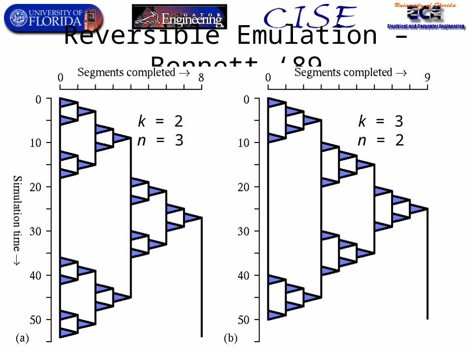
Reversible Emulation – Bennett ‘89
k = 2n = 3
k = 3n = 2
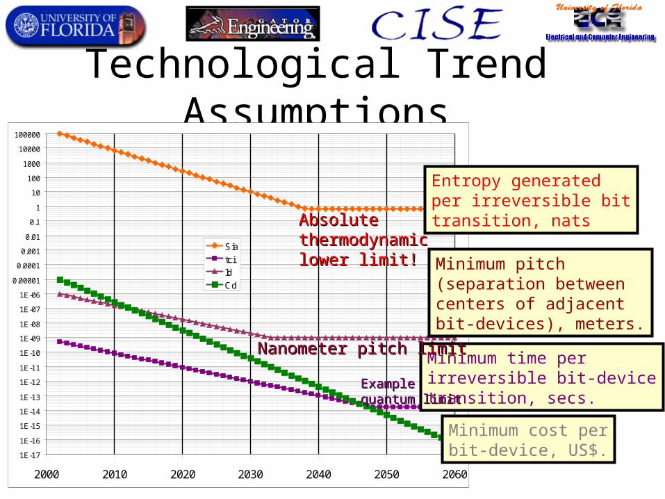
Technological Trend Assumptions
1E-17
1E-16
1E-15
1E-14
1E-13
1E-12
1E-11
1E-10
1E-09
1E-08
1E-07
1E-06
0.00001
0.0001
0.001
0.01
0.1
1
10
100
1000
10000
100000
2000 2010 2020 2030 2040 2050 2060
Sia
tci
ld
Cd
Entropy generatedper irreversible bittransition, nats
Minimum time perirreversible bit-devicetransition, secs.
Minimum pitch (separation between centers of adjacent bit-devices), meters.
Minimum cost perbit-device, US$.
Absolute Absolute thermodynamicthermodynamiclower limit!lower limit!
Nanometer pitch limitNanometer pitch limit
Example Example quantum limitquantum limit
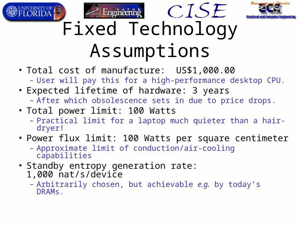
Fixed Technology Assumptions
• Total cost of manufacture: US$1,000.00– User will pay this for a high-performance desktop CPU.
• Expected lifetime of hardware: 3 years– After which obsolescence sets in due to price drops.
• Total power limit: 100 Watts– Practical limit for a laptop much quieter than a hair-dryer!
• Power flux limit: 100 Watts per square centimeter– Approximate limit of conduction/air-cooling capabilities
• Standby entropy generation rate: 1,000 nat/s/device– Arbitrarily chosen, but achievable e.g. by today’s DRAMs.
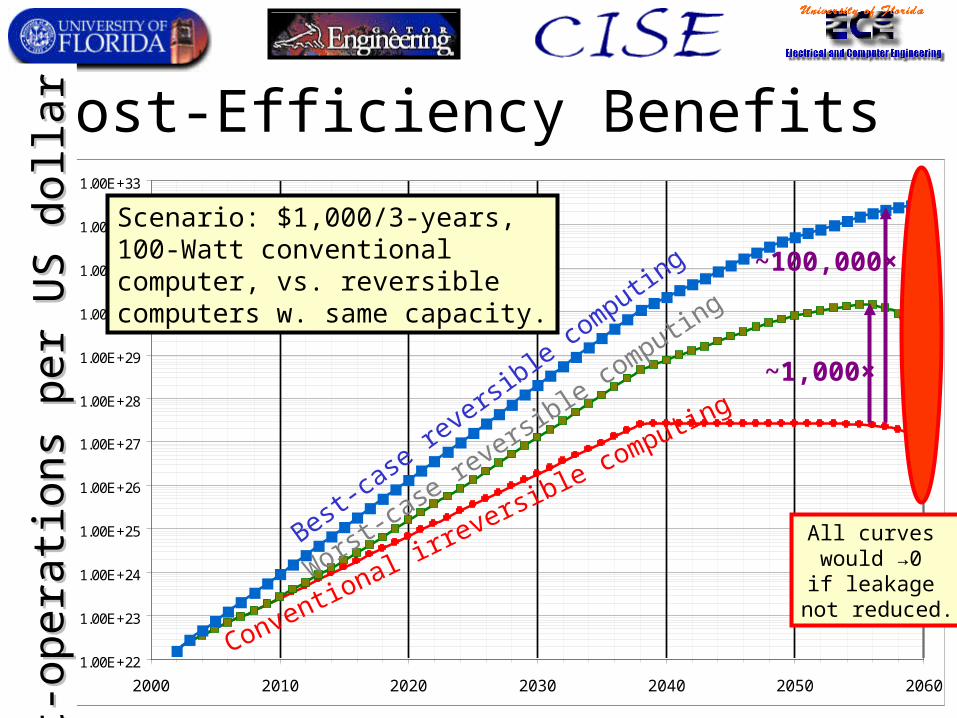
Cost-Efficiency Benefits
1.00E+22
1.00E+23
1.00E+24
1.00E+25
1.00E+26
1.00E+27
1.00E+28
1.00E+29
1.00E+30
1.00E+31
1.00E+32
1.00E+33
2000 2010 2020 2030 2040 2050 2060
Bit
-ope
rati
ons
per
US
dol
lar
Bit
-ope
rati
ons
per
US
dol
lar
Conventional irreversib
le computing
Worst-cas
e revers
ible computin
g
Best-ca
se rev
ersible
computin
g
Scenario: $1,000/3-years, 100-Watt conventional computer, vs. reversible computers w. same capacity.
All curves would →0 if leakage
not reduced.
~1,000×
~100,000×
Minimizing Entropy Generation in Adiabatic FET Operations
Taking leakage-voltage tradeoff into account
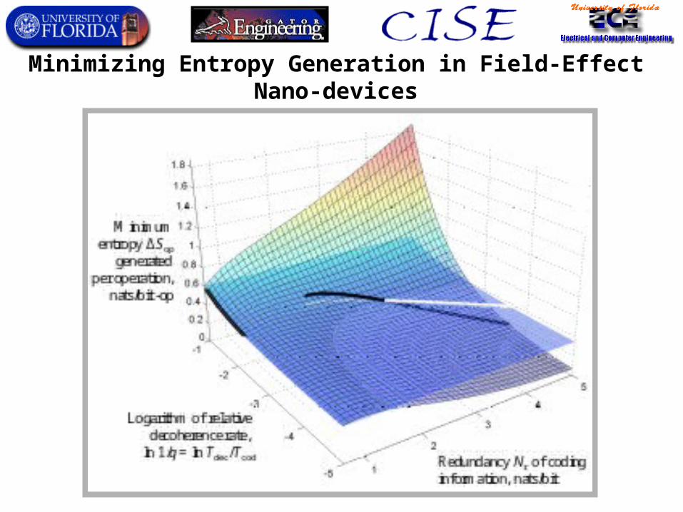
Minimizing Entropy Generation in Field-Effect Nano-devices
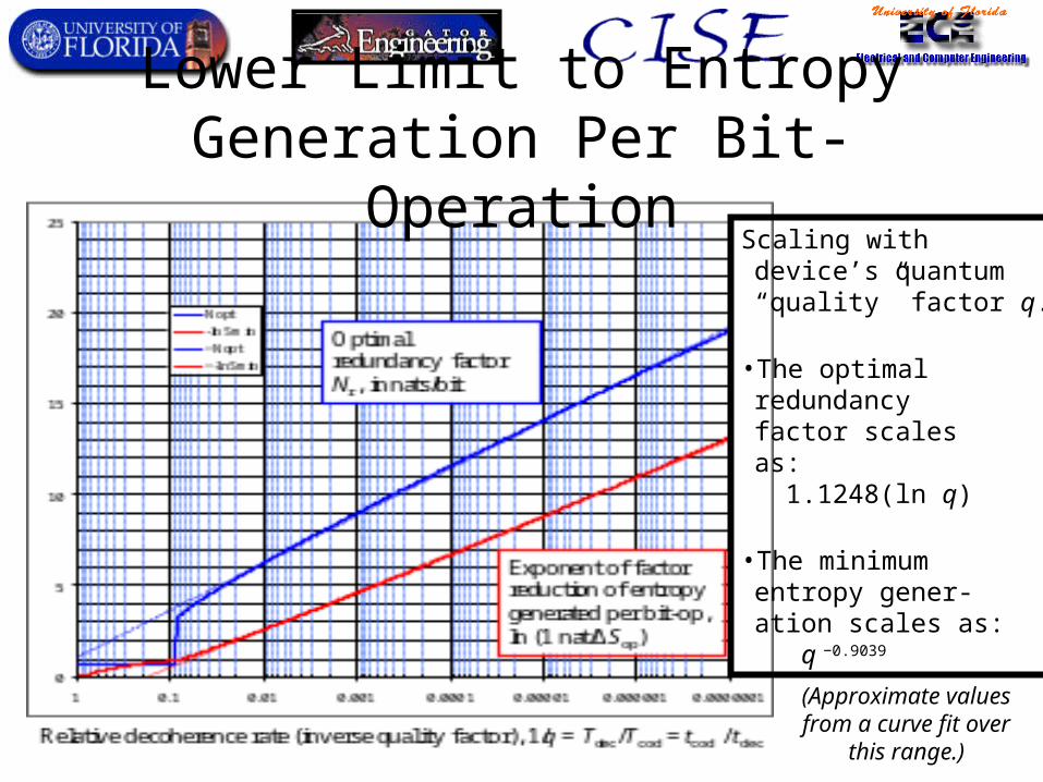
Scaling withdevice’s quantum“quality” factor q.
• The optimal redundancyfactor scales as: 1.1248(ln q)
• The minimumentropy gener-ation scales as: q −0.9039
Lower Limit to Entropy Generation Per Bit-Operation
(Approximate valuesfrom a curve fit over
this range.)
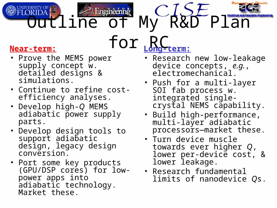
Outline of My R&D Plan for RCNear-term:• Prove the MEMS power
supply concept w. detailed designs & simulations.
• Continue to refine cost-efficiency analyses.
• Develop high-Q MEMS adiabatic power supply parts.
• Develop design tools to support adiabatic design, legacy design conversion.
• Port some key products (GPU/DSP cores) for low- power apps into adiabatic technology. Market these.
Long-term:• Research new low-leakage
device concepts, e.g., electromechanical.
• Push for a multi-layer SOI fab process w. integrated single-crystal NEMS capability.
• Build high-performance, multi-layer adiabatic processors—market these.
• Turn device muscle towards ever higher Q, lower per-device cost, & lower leakage.
• Research fundamental limits of nanodevice Qs.
By Michael Frank
With device sizes fast approaching atomic-scale limits, ballistic circuits that conserve information will offer the only possible way to keep improving energy efficiency and therefore speed for most computing applications.
To besubmitted
toScientific
American?


![CIS medical medical ï279-0012 3-70 A4-l TEL : 047-374-3100 ... · made Japan . CISE QR2— CISEläs 145mm 42 mm 35 25 CISE (01 • 99)/ YL CISE [mm] Y (CISE) 26.6 CISE 30 43.8 18.0](https://img.pdfslide.net/doc/110x75/5f4696d3563f08072f1ba13d/cis-medical-medical-279-0012-3-70-a4-l-tel-047-374-3100-made-japan-cise.jpg)