Embed Size (px)
Citation preview
1
The Impact of Award Uncertainty on Settlement Negotiations
Eric Cardella1 Carl Kitchens2
Texas Tech University Florida State University
February 25, 2016
Abstract
Legal disputes are often negotiated under the backdrop of an adjudicated award. While settlements are
common, they are not universal. In this paper, we empirically explore how uncertainty in adjudicated awards
impacts settlement negotiations. To do so, we develop an experimental design to test how increases in
variance and positive skewness of the award distribution impact negotiations and settlement rates. We find
increases in variance decrease settlement rates, while increases in skewness generally increases settlement
rates. We also gather individual measures of risk aversion and prudence, and incorporate these measures into
the analysis to test for heterogeneous treatment effects. Overall, our results suggest that highly variable
adjudicated awards can contribute to the excess use of inefficient litigation, while more positively skewed
awards can reduce the use of inefficient litigation.
We thank David Cooper, Cary Deck, Martin Dufwenberg, Mike Eriksen, Taylor Jaworski, Harris Schlesinger,
Mike Seiler, Alec Smith, Mark Van Boening, and conference participants at the 2013 Western Economics Association
meetings, the 2013 Southern Economic Association meetings, 2013 Economic Science Association meetings, and the
2014 Public Choice Society meetings for helpful comments. We are grateful to Rochester Institute of Technology, the
University of Mississippi, and L. Charles Hilton Jr. Center for the Study of Economic Prosperity and Individual
Opportunity at Florida State University for financial support. 1 Rawls College of Business, Texas Tech University, Lubbock, TX 79409; Telephone: (858) 395-6699; Email:
[email protected]. 2 Department of Economics, Florida State University, 239 Bellamy Building, Tallahassee, FL 32306;
Email:[email protected].

2
1 Introduction
Settlement negotiations between disputing parties are often carried out under the backdrop of an
adjudicated award if the parties fail to settle. Examples of such disputes include: punitive damages,
patent infringements, breaches of contract, antitrust, labor arbitration, and eminent domain.
Litigation dispute models of this type abound, and while these models differ in their informational
structures and underlying assumptions, a common feature is costly litigation when settlement
negotiations fail; consequently, it is often beneficial for both parties to negotiate a settlement and
avoid litigation.3 While settlements are common in practice, they are not ubiquitous.4 Given the
(possible) inefficiency associated with excessive and costly litigation, it is important to understand
the potential sources of settlement failure (as discussed by Babcock & Lowenstein, 1997).
In legal disputes, there is likely to be substantial variability and unpredictability in the adjudicated
award, especially those handed down by juries. As an epitomizing example, in 1994 Stella Liebeck
sued McDonald’s after accidentally spilling hot coffee on herself. After failing to reach a settlement,
a New Mexico, USA jury awarded Ms Liebeck over $2.86 million to cover medical expenses and
punitive damages.5 Empirical evidence of substantial variation and positive skewness across court
awards has been documented in several studies (e.g., Kahneman et al., 1998, Black et al., 2005;
Kaplan et al., 2008; and Mazzeo et al., 2013).6 Sunstein et al. (2002) highlight the likely presence
of variability in adjudicated awards in their concluding remarks where they state: “the result [of the
award process] is a decision that is unreliable, erratic, and unpredictable.” (p. 241)
We posit that the degree of uncertainty in adjudicated awards, either real or perceived, may
impact settlement negotiation behavior and, consequently, the likelihood that a settlement is
reached. In this paper, we develop a laboratory experiment that enables us to empirically investigate
3 We refer readers to Posner (1973), Gould (1973), Shavell (1982), P’Ng (1983), Bebchuk (1984), Nalebuff (1987),
and Schweizer (1989) for seminal legal dispute models. 4 For example, Kaplan et al. (2008) document only a 70 percent settlement rate in labor disputes in Mexico. Similar
percentages of settlement in different settings are documented in Trubek et al. (1983) and Williams (1983). 5 On appeal, the verdict was reduced to $640,000 although a private settlement was eventually reached. 6 Specifically, Kaplan et al. (2008) note that court awards are often more variable than expected in labor disputes in
Mexico, in the sense that they are lower than settlements of similar cases. Mazzeo et al. (2013) found that in a sample
of 340 patent infringement cases, the top eight court awards accounted for over 47 percent of all damages awarded,
which is suggestive of substantial variance and positive skewness. Similarly, Black et al. (2005) consider a sample of
closed insurance claims in Texas from 1988 to 2002, and they find that approximately 5 percent of claims account for
42 percent of payouts with jury awards tending to be excessively positively skewed.
3
how increases in variance and skewness of the adjudicated award distribution impact settlement
negotiation behavior, settlement rates, and the degree of inefficient litigation.
Changes in the distribution of awards (assuming the mean is unchanged) would not be expected
to impact negotiation behavior and settlement rates under the assumption that the involved agents
are risk-neutral (e.g., P’Ng, 1983; Bebchuk, 1984; Nalebuff, 1987; and Schweizer, 1989). However,
over the past several decades, a plethora of research has documented decision-making inconsistent
with risk-neutrality.7 Specifically, the role of risk aversion has been explored in various bargaining
environments.8 More recently, several studies have experimentally documented evidence that agents
exhibit prudent behavior (Deck & Schlesinger, 2010; 2014; Ebert & Wiesen, 2011; 2014 Maier &
Rüger, 2012; and Noussair et al., 2014). As originally termed by Kimball (1990), prudence refers to
a convex marginal utility function or an aversion to increases in downside risk (Menezes et al.,
1980); prudent behavior is relevant in our context because prudence implies skewness seeking
(Ebert & Wiesen, 2011). That is, prudent agents have a preference for more positively skewed
distributions. If disputing parties exhibit non risk-neutral behavior, then changes in the variance or
skewness of the court award are likely to affect the disputing parties’ settlement offers, which can
then impact the likelihood of settlement (Posner, 1973).
Ideally, one would want to explore the impact of changes in variance and skewness of adjudicated
awards on settlement negotiations using empirical case data. However, this poses some obvious
challenges, the most significant of which is the inability to observe the degree of uncertainty in the
underlying court award distribution. Second, we may not observe rejected settlements, which would
make it difficult to infer welfare implications due to selection. Third, it is often difficult to observe
offers in the settlement negotiation process, as well as the associated reservation values of disputing
parties. Given these challenges, a controlled experiment is both a suitable and necessary approach
to rigorously examine how award uncertainty impacts settlement negotiations. We develop an
experimental design that allows us to systematically manipulate the degree of uncertainty in the
underlying award distribution while holding other factors constant. Moreover, we also observe the
negotiation stage and settlement rates, which enables us to analyze the welfare effects of changes in
7 We will not attempt to cite all relevant studies. Rather, we reference Cox & Harrison (2008) and Dave et al. (2010),
who provide comprehensive, although not exhaustive, reviews of this extensive body of literature. 8 Examples include: Shavell (1982) in the context of pretrial negotiation; Grossman & Katz (1983) in plea
bargaining; Kihlstrom & Roth (1982) in insurance contracts; Deck & Farmer (2007) in arbitration; and White (2008) in
alternate-offer negotiations.

4
award uncertainty. Lastly, we are able to elicit individual risk preferences and correlate these
measures with the propensity to litigate. As such, our study joins a growing body of literature using
a controlled experimental environment to better understand legal disputes.9
In our experiment, we consider a stylized, bilateral settlement negotiation game where the two
involved parties are given an opportunity to negotiate a settlement under the backdrop of an
adjudicated award. If negotiations fail and a settlement is not reached, then one of the negotiating
parties receives the adjudicated court award, which consists of a random draw from a known but
uncertain award distribution. We then systematically increase the variance (or skewness) of the
award distribution across experimental treatments, while holding the mean and skewness (and
variance) constant. By comparing across treatments, we can identify how increases in variance and
skewness impact the negotiation behavior of each party (i.e., offers and propensities to accept offers)
and, ultimately, settlement rates. Additionally, we elicit individual measures of risk aversion and
prudence (a proxy for skewness seeking) using the binary choice lottery method developed by
Eeckhoudt & Schlesinger (ES henceforth) (2006). This element of the design allows us to associate
behavior in the negotiation task with relative measures of risk aversion and prudence, and provide
a more robust analysis of possible differential treatment effects based on individual risk preferences.
Overall, we find that increases in the variance of the court award result in decreased settlement
rates, while increases in skewness generally increased settlement rates. Perhaps most importantly,
we find that even after controlling for interactions when litigation would be efficient, relatively high
levels of variance in the adjudicated award leads to excessive, inefficient litigation, while some
positive skewness leads to lower levels of inefficient litigation. Moreover, our main results are
generally robust across both a contextually framed settlement negotiation and an abstractly framed
setting, which, in our view, increases the robustness of our key findings.
To reduce the burden of excess litigation, several states have enacted tort reforms that cap
punitive and/or non-economic damages, or have changed liability laws that may alter the incentives
of plaintiffs, defendants, and insurers.10 Closely related to our work is the prior research that has
investigated the effect of damage caps on litigation. Such studies include Browne & Puelz (1999)
9 For recent examples see Croson & Mnookin (1997), Babcock & Pogarsky (1999), Pogarsky & Babcock (2001),
Babcock & Landeo, (2004), Pecorino & Van Boening (2004; 2010), Landeo et al. (2007), and Collins & Isaac (2012) 10 We refer readers to the American Tort Reform Association (ATRA) for a thorough discussion of the specific
details of individual reforms at the state level (http://www.atra.org/legislation/states).

5
who show that damage caps tend to reduce both the value of claims and the frequency of frivolous
suits. Similarly, Avraham (2007) uses medical malpractice suits and finds that award caps on pain
and suffering lead to reduced settlement payments and fewer litigated cases. However, Donohue &
Ho (2007) and Durrance (2010) find no evidence that damage caps result in fewer medical
malpractice claims. Experimentally, Babcock & Pogarsky (1999) find that a “binding” damage cap
tends to increase settlement rates; yet, in a follow-up study, Pogarsky & Babcock (2001) find that a
very large “non-binding” cap actually tends to decrease settlement rates. While these prior studies
suggest that the degree of award uncertainty can impact settlement negotiations, it is not possible to
identify the effects resulting from changes in uncertainty from changes in the expected value of the
award, since the imposition of award caps simultaneously decreases the mean, variance, and
skewness of the award distribution. However, in our design, we hold constant the mean and variance
(skewness), which enables us to separately identify the effect of increased skewness (variance) on
settlement negotiations; we view this as an important complement to this extant body of research
related to damage caps.
Previous research has suggested that self-serving bias may be one channel that contributes to
settlement failure (e.g., Loewenstein et al., 1993; Babcock et al., 1995; Babcock & Loewenstein,
1997; and Babcock & Pogarsky, 1999). The general idea behind the theory is that under the presence
of an uncertain and unknown award, plaintiffs hold more optimistic beliefs than the defendant
regarding the likely outcome; consequently, this discrepancy in beliefs can lead to settlement failure.
In our design, we eliminate this self-serving bias channel as a source of settlement failure by making
the award distribution known to both parties. Yet, even with a commonly known award distribution,
we document a substantial degree of settlement failure, and find that changes in the variance and
skewness of the award distribution significantly impact inefficient settlement failure. Thus, we
identify another possible channel through which award uncertainty can influence settlement
negotiations.
More broadly, we believe this paper contributes to several areas of existing literature. Regarding
the literature on legal disputes, much of the prior work has focused on the role of information
asymmetries, credibility, and court cost allocations in contributing to settlement failures. This paper
suggests, as an alternative contributing explanation, that the degree of uncertainty in the adjudicated
award can impact settlement rates and the use of inefficient litigation. Furthermore, our study
contributes to the small existing literature on ultimatum bargaining with an outside option (see

6
Croson et al., 2003; and Anbarci & Feltovich, 2013 for reviews). These papers have examined cases
where the size of the pie is random and/or the outside option is fixed, while we study ultimatum
bargaining with an uncertain outside option. Lastly, we join a recent series of papers that explore
how prudence can affect economic behavior (see Noussair et al., 2014; and Ebert & Wiesen, 2014
for reviews); specifically, our study provides additional experimental evidence that subjects exhibit
prudent behavior, which can influence negotiation behavior.
2 Experimental Design
2.1 The Settlement Negotiation Task
To provide participants with context in the experimental task, the settlement negotiation was
framed to participants in a common legal environment – a land acquisition game under the presence
of eminent domain (ED henceforth).11 In particular, the framing is intended to represent the
following setting: An individual agent, the seller, owns a plot of land, and a buyer wants to acquire
it from the seller and has been granted the power of ED.12 We assume the value of the land to the
buyer is sufficiently high that it remains profitable to acquire the land through the use of ED; thus,
invoking ED on the seller is a credible threat. In an attempt to avoid the court costs associated with
using ED, the buyer first tries to negotiate a settlement price with the seller. If a settlement is not
reached, the buyer files suit to acquire the land via ED; both parties proceed to court where the land
is granted to the buyer in exchange for “just” compensation, as determined by the court. In the
context of a more general legal dispute, the seller could be viewed as the plaintiff, the buyer as the
liable defendant, and the just compensation as the adjudicated court award.
In the experiment, all monetary amounts are in experimental currency units (ECU), which are
converted into dollars at a rate of 10 ECU = $1. Buyers are informed that their value for acquiring
11 Eminent domain is the right of the state to acquire a property in exchange for a court determined fair market value
under the takings clause of the 5th Amendment of the US Constitution. In 2005, the U.S. Supreme Court ruled in favor
of the City of New London, CT in Kelo vs. New London, which extended the right of ED to private firms and developers
that satisfy the public use requirement. The extended right of ED to private firms, as well as the possible inefficiencies
resulting from its use, has led to a renewed interest amongst economists and legal scholars. We refer interested readers
to GAO (2006), Miceli & Sergerson (2007), Lopez et al. (2009), Shavell (2010), Turnbull (2012), and Kitchens (2014)
for more detailed discussions of ED rights, usages, and corresponding legal issues. 12 One possible concern with using contextually rich framing in is that the main findings may be an artifact of the
specific framing and, thus, may not generalize to other relevant negotiation settings involving an uncertain outside
option. To address this concern and provide some evidence of the robustness of our main results, we run additional
treatments where we use completely abstract framing. In general, we are able to replicate our main results with abstract
framing. We discuss these additional treatments and provide more detail regarding the results in Section 4.

7
the land is 200 ECUs; sellers are informed that their reservation value for the land is 0 ECUs (for
simplicity). The litigation cost of using ED is set to 50 ECUs. The negotiation phase consists of an
“ultimatum” style bargaining protocol, where the buyer makes a take-it or leave-it settlement offer,
and the seller decides whether to accept or reject the buyer’s offer. If the seller accepts, then the
property is transferred at the accepted price; otherwise, it is transferred via ED in exchange for the
awarded compensation, which is a draw from the uncertain award distribution.
Table 1: Court Award Distributions for Each of the Five Treatments
In the experiment, we consider five different award distributions, each of which corresponds to
one of the five experimental treatments. In each of the five award distributions, the mean is held
constant at 100 ECUs. However, the distributions differ across two dimensions: (i) variance and (ii)
skewness. Table 1 displays the award distributions and their corresponding degrees of variance and
80 50%
120 50%
0 15%
40 25%
100 20% 100 4800 0
160 25%
200 15%
0 50%
200 50%
0 4%
40 15%
60 36%
80 15%
140 25%
500 5%
0 1%
80 60%
100 37% 100 10000 7.87
500 1%
1000 1%
Variance SkewnessTreatment
Low Variance
(L-Var) 100 400 0
Court Award
Amount
(ECU)
Chance of
Court AwardMean
3.14Med Skewness
(M-Skew)
100 10000 0
Med Variance
(M-Var)
High Variance /
Low Skewness
(H-Var / L-Skew)
High Skewness
(H-Skew)
100 10000

8
skewness.13 Looking at Table 1, we see that across the three variance treatments the three
distributions are symmetric with zero skewness, but the variance is increasing via a mean preserving
spread.14 Similarly, looking across skewness treatments, the mean and variance of the three
distributions are held constant, while the distributions become more positively skewed. By
comparing the bargaining behavior across these three variance (skewness) treatments, we are able
to explore how increases in variance (skewness) of the award affect negotiation behavior and
settlement rates.
In terms of payoffs, when an agreement is reached, the buyer receives his value of 200 ECUs
minus the accepted price, while the seller receives the accepted price. In the event of a settlement
failure, ED is used and the seller receives the randomly drawn court award; the buyer receives a
fixed payment of 50 ECUs. This fixed 50 ECU payment to the buyer is equivalent to the buyer
paying the 100 ECU expected court award plus the entire 50 ECU cost of ED, which results in a
fixed net payoff of: 200 ECUs – 100 ECUs – 50 ECUs = 50 ECUs. The primary motivation for
implementing a fixed buyer payment when there is settlement failure is that, from a design
standpoint, a fixed payment allows us to consider very positively skewed award distributions with
large (possible) awards to the seller, e.g., 500 ECUs ($50) and 1,000 ECUs ($100), without inducing
the possibility of large negative payoffs to the buyer, which would be difficult to impose in an
experimental setting.15 From a conceptual standpoint, this allows us to explore how the presence of
very positively skewed award distributions impacts the seller’s (or plaintiff’s more generally)
behavior in the settlement negotiation and, ultimately the likelihood that a settlement is reached. A
possible limiting implication of imposing a fixed payment for the buyer is that it eliminates the
payoff uncertainty on the side of the buyer when there is a settlement failure. However, it is
13 For the sake of administering payments in the experiment and making the design easier to understand for the
participants, we used only integer values for the probabilities. As a result, three of the values reported in Table 1 are
rounded approximations of their exact values. Specifically, the mean of distribution M-Skew is 99.6, the variance of
distribution M-Skew is 9,976, and the variance of distribution H-Skew is 10,040. Given that none of these three exact
values differs by more than .4% from its reported value in the table, we assume the observed behavior in treatments M-
Skew and H-Skew is equivalent to the behavior that would result if the mean and variance of the distributions in M-
Skew and H-Skew were the exact values reported in Table 1. 14 By considering some limited uncertainty in L-Var, we hold constant the fact that there was some uncertainty
present in all distributions. This helps ensure that any observed differences among L-Var, M-Var, and H-Var are not
merely a result of the discontinuous jump of going from no uncertainty to some uncertainty. 15 Alternatively, we could have made buyers responsible for paying the court award and then implemented some
sort of bankruptcy rule. However, this would have limited the liability of buyers, which would have distorted the
incentives of the buyers. We could have also just provided each buyer with a $100 endowment, although this would
have been a very costly option and may have induced other drawbacks like wealth and house money effects.

9
important to note that the fixed payment does not induce risk-neutral behavior from the buyers as
they still face strategic risk that arises from the seller’s response to their offer.16
The ultimatum nature of the bargaining process is a stylized feature of our settlement negotiation
process. Certainly ED negotiations, and settlement negotiations more generally, could involve a
more dynamic bargaining process of offers and counter-offers. However, it is likely that settlement
negotiations would, at some point, culminate in an ultimatum offer. Thus, even if the dispute setting
featured a more complex negotiation framework, the ultimatum offer from the buyer could be
thought of as capturing the last round of the negotiation prior to litigation.17
2.2 Lottery Choice Task
After completing the ED task, each participant completes an incentivized lottery choice task
consisting of a series of 30 questions. A detailed description of the elicitation method and a list of
all 30 lottery pairs are provided in Appendix A. The motivation for the lottery choice task is to elicit
measures of risk aversion and prudence for each participant.
For the elicitation of risk aversion, we consider two different instruments. The first, which we
denote as the ES-risk measure, consists of 10 lottery questions based on the method developed by
ES (2006);18 the corresponding ES-risk measure is the number of instances (out of 10) where the
individual selected the less risky option of the lottery pair. The second measure of risk aversion is
16 One could view the fixed payment as representing a setting where the liable defendant is assumed to be acting in
a risk-neutral manner, and effectively approaches the settlement negotiation under the backdrop of being required to
pay an amount equal to the expected court award when there is settlement failure. In some dispute settings, it may be
reasonable to think the liable defendant (e.g., a large company or a government agency) is acting in a risk-neutral
manner, especially when the defendant is repeatedly involved in settlement deputes. Alternatively, the fixed payment
could also be viewed in the context of decoupled liability, where the amount the buyer (or defendant) pays can differ
from the amount the seller (plaintiff) receives (see Schwartz, 1980; Salop & White, 1986 for a discussion of decoupled
liability in the context of antitrust settlements, and Polinsky & Che, 1991; Chu & Chien, 2007 for theoretical models). 17 This paper is certainly not the first to use an ultimatum bargaining protocol in the context of studying settlement
negotiations. Other prominent examples include Babcock & Landeo (2004), Pecorino & Van Boening (2004); (2010),
Landeo et al. (2007), and, more specific to our context, Shavell (2010) who models the ED bargaining protocol with
only one take-it or leave-it offer made by the buyer. As an anecdotal example, TransCanada, which has been granted
the right to use ED to construct the Keystone Pipeline, negotiated with one farmer for several years before threatening
the use of ED; in the news article, the farmer was quoted as saying, “We were given three days to accept their offer, and
if we didn't, they would condemn the land and seize it anyway” (Brasch, May 19, 2013). 18 We refer interested readers back to this paper, or a follow-up paper by Eeckhoudt et al. (2009), for a more formal
and thorough discussion of how choices in these lottery choice problems can be used to characterize the various orders
of risk attitudes. Our implementation of the elicitation task is similar in spirit to the prior studies that have used this
lottery choice method (Deck & Schlesinger, 2010; 2014; Ebert & Wiesen, 2011; 2014; Maier & Rüger, 2012; and
Noussair et al., 2014).

10
the well-known 10-question Holt & Laury (2002) method, which we call the HL-risk measure.19 For
the elicitation of prudence, we use 10 different lottery questions based on the ES (2006) method;
the corresponding measure of prudence, which we call ES-prudence, is the number of instances (out
of 10) where the individual selected the more prudent lottery option.
2.3 Experimental Procedure
Experimental sessions were initially conducted at the Mississippi Experimental Research
Laboratory (MERL) at the University of Mississippi in March and June 2013. We also conducted
follow-up sessions at the XS/FS laboratory at Florida State University in January and February of
2016 using both the contextualized framing and a completely abstract framing. The motivation for
running these follow-up sessions was to test for possible framing effects. We describe the abstract
framing conditions in more detail, and summarize the main results from the abstract framing
conditions in Section 4. In total, 21 sessions were conducted with a total of 332 participants. The
entire experiment was computerized, and the software was programmed in z-Tree (Fischbacher,
2007). Participants were randomly assigned to either the role of buyer or seller, and they remained
in this role the entire study. Copies of the role-specific experimental instructions are presented in
Appendix B. Participants first completed five rounds of the ED task, followed by the lottery task.20
We used a within-subjects design where the five rounds of the ED task corresponded to the five
different experimental treatments. Each participant was randomly and anonymously paired with a
participant of the opposite role, and was randomly re-matched with a different participant each
round. The advantage of the within-subjects design is that it allows us to analyze individual
differences in negotiation behavior as the award distribution changes. However, there is a potential
for order effects when using a within-subjects design, which can impact the comparison across
treatments. To help mitigate possible order effects, we used three different randomly drawn
sequences for the ordering of the five treatments.21
19 One potential drawback of the Holt & Laury method is that individuals are free to choose between Option A and
Option B in each of the 10 gambles, which may induce multiple switch points (e.g., Jacobson & Petrie, 2009; and Dave
et al., 2010). This is problematic for inferring a measure of risk aversion for such individuals, as the Holt & Laury
method requires a unique switch point for eliciting risk aversion (see Charness et al., 2013 for a discussion). 20 By having all subjects complete the lottery task second, it is possible that the results from the ED negotiation task
may have impacted decisions in the lottery task. Given that our primary research questions relate to outcomes in the ED
task, we chose to run the ED task first, thus mitigating the potential for order effects on the ED task. 21 With five different treatments, it was not feasible to consider all possible unique orderings (120 different orders).
As an alternative, we ran 3 different orderings, which were as follows: (1) H-Skew; H-Var/L-Skew; L-Var; M-Var; M-

11
We implemented a modified strategy method in the ED task. In each round, the buyer was asked
to state his price offer; contemporaneously, the seller was asked to state the minimum price she was
willing to accept to avoid going to court, which we refer to as the seller’s minimum willingness to
accept (MWA). What we denote as the seller’s MWA is analogous to what Babcock & Pogarsky
(1999) denote as the plaintiff’s reservation value, and can be similarly interpreted as the seller’s
“bottom line” in the negotiation phase.22 After the buyer made his offer and the seller stated her
MWA, the buyer’s offer was revealed to the seller. If the offer was greater than or equal to the stated
MWA, a settlement was reached at the buyer’s offer. If the buyer’s offer was lower than the seller’s
MWA, there was a settlement failure and ED was used. Buyers were only informed of whether their
offer was accepted or rejected and not the MWA for sellers. This information feedback protocol is
analogous to the feedback each party would receive in a direct response ultimatum bargaining
format. The benefit of implementing this modified strategy method is that it allows us to gather
more refined information about how the variance and skewness of the award impact sellers’ MWA.
When there was a settlement failure, the buyer and the seller were not informed at that time of
the actual realized court award draw. This was done to help limit wealth and house money effects,
which could possibly influence behavior in subsequent rounds or in the lottery task. Sellers were
informed in the instructions that buyers would pay a fixed amount for the land when there was a
settlement failure and ED was used, but they were not informed of the amount, which helps ensure
that their stated MWA was not influenced or biased by knowing the exact amount of the buyer’s
fixed payment. Implementing a fixed payment scheme for the buyers, while not explicitly conveying
the amount to sellers, should not generate seller behavior that is systematically inconsistent from
the case where the buyer pays the actual realized award.
After finishing the ED task, participants completed the risk elicitation lottery task. The 10 ES-
risk and 10 ES-prudent lottery questions were presented in random order, and the lottery display
Skew, (2) M-Var; L-Var; M-Skew; H-Var/L-Skew; H-Skew, (3) H-Var/L-Skew; M-Var; M-Skew; H-Skew; L-Var. In
the analysis, we test for order effects and find essentially no statistically significant evidence of order effects. 22 In essence, the seller is stating a threshold strategy such that for all offers less than her stated MWA, she would
reject, while all offers greater than or equal to her stated MWA she would accept. The seller’s strategy should follow
this type of threshold pattern, so this modified strategy method should yield results consistent with the direct response
method. For a more general discussion comparing the strategy vs. direct response method, we refer readers to a recent
survey by Brandts & Charness (2011). The majority of the studies in their survey do not find significant differences
between the two methods. Furthermore, even if the implementation of the strategy method does impact the level of the
MWA threshold, as long as this is not correlated with the different treatments, our relative comparison of the MWA
threshold across treatments remains unaffected.

12
was also randomized.23 After completing both tasks, participants were privately paid their earnings.
To ensure incentive compatibility for both tasks, all participants were randomly paid for either one
randomly selected round from the ED task or one randomly selected lottery problem, which was
determined by the outcome of a physical randomization device. The average session lasted 45
minutes and the average earnings were approximately $19/participant.
2.4 Predictions in the Settlement Negotiation Task with an Uncertain Outside Option
In our setting, the negotiation phase consists of an ultimatum bargaining environment with an
outside option for each party – for the buyer, the outside option is 50 ECUs (the net payment if ED
is used), and for the seller, the outside option is the draw from the award distribution. The setup of
our settlement negotiation environment follows closely in spirit to the one modeled in Babcock &
Pogarsky (1999) and Pogarsky & Babcock (2001).24 As a backdrop for analyzing our settlement
negotiation setting with an uncertain court award, it is pedagogical to first consider a similar
negotiation environment with a certain court award. In particular, if the court award was a certain
100 ECUs (the expected value of the award distributions we consider), then the predicted behavior
and corresponding outcome are rather straightforward. Applying backward induction, it would be
optimal for the seller to accept any offer greater than or equal to the outside option of 100 ECUs,
and reject all other offers; that is, the seller’s MWA would be 100 ECUs. Anticipating this, the buyer
then offers 100 ECUs, which would be accepted by the seller. Thus, we would predict 100%
settlement rate at a price of 100 ECUs.25
23 One random sequence for these lotteries was drawn prior to the experiment, and all participants saw the same
sequence. In addition, all lotteries were presented in their reduced form. This differs from most of the previous
applications of this lottery method, which present the lotteries in their compound forms (when warranted). However,
Maier & Rüger (2012) use the reduced form representations, and the observed frequencies of risk averse and prudent
choices are generally in line with the results from studies that use the compound representations. 24 A few prior studies have considered ultimatum bargaining games with an outside option (Knez & Camerer, 1995;
Pillutla & Murnighan, 1996; Boles et al., 2000; Croson et al., 2003; and Schmitt, 2004); however, these prior studies
consider only certain outside options, while we consider an ultimatum bargaining setting with an uncertain outside
option of varying degrees of variance and skewness. 25 Obviously this analysis ignores the possibility that the seller and/or the buyer may be motivated by other-regarding
or social preferences, which generally include fairness concerns, reciprocity, and efficiency concerns. Such preferences
could motivate the behavior of sellers and/or buyers and possibly lead to an outcome that differs from the buyer making
an offer equal to the outside option court award and the seller accepting. While the presence of other-regarding or social
preferences have been extensively documented in prior literature, we abstract away from such preferences and focus on
how risk preferences of the seller may impact behavior with an uncertain outside option. Furthermore, as long as such
preferences are independent of the degree of uncertainty in the outside option (assuming a constant expected court
award), then our relative comparison across treatments with varying degrees of uncertainty remains valid.
13
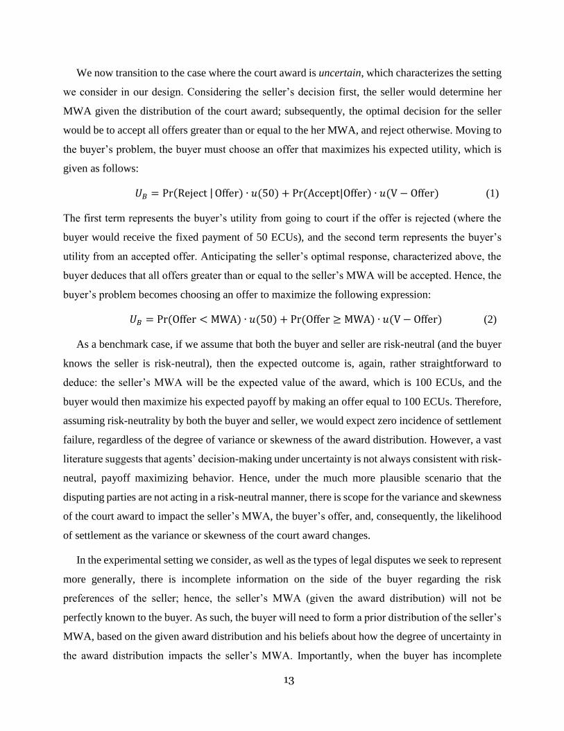
We now transition to the case where the court award is uncertain, which characterizes the setting
we consider in our design. Considering the seller’s decision first, the seller would determine her
MWA given the distribution of the court award; subsequently, the optimal decision for the seller
would be to accept all offers greater than or equal to the her MWA, and reject otherwise. Moving to
the buyer’s problem, the buyer must choose an offer that maximizes his expected utility, which is
given as follows:
𝑈𝐵 = Pr(Reject | Offer) ∙ 𝑢(50) + Pr (Accept|Offer) ∙ 𝑢(V − Offer) (1)
The first term represents the buyer’s utility from going to court if the offer is rejected (where the
buyer would receive the fixed payment of 50 ECUs), and the second term represents the buyer’s
utility from an accepted offer. Anticipating the seller’s optimal response, characterized above, the
buyer deduces that all offers greater than or equal to the seller’s MWA will be accepted. Hence, the
buyer’s problem becomes choosing an offer to maximize the following expression:
𝑈𝐵 = Pr (Offer < MWA) ∙ 𝑢(50) + Pr (Offer ≥ MWA) ∙ 𝑢(V − Offer) (2)
As a benchmark case, if we assume that both the buyer and seller are risk-neutral (and the buyer
knows the seller is risk-neutral), then the expected outcome is, again, rather straightforward to
deduce: the seller’s MWA will be the expected value of the award, which is 100 ECUs, and the
buyer would then maximize his expected payoff by making an offer equal to 100 ECUs. Therefore,
assuming risk-neutrality by both the buyer and seller, we would expect zero incidence of settlement
failure, regardless of the degree of variance or skewness of the award distribution. However, a vast
literature suggests that agents’ decision-making under uncertainty is not always consistent with risk-
neutral, payoff maximizing behavior. Hence, under the much more plausible scenario that the
disputing parties are not acting in a risk-neutral manner, there is scope for the variance and skewness
of the court award to impact the seller’s MWA, the buyer’s offer, and, consequently, the likelihood
of settlement as the variance or skewness of the court award changes.
In the experimental setting we consider, as well as the types of legal disputes we seek to represent
more generally, there is incomplete information on the side of the buyer regarding the risk
preferences of the seller; hence, the seller’s MWA (given the award distribution) will not be
perfectly known to the buyer. As such, the buyer will need to form a prior distribution of the seller’s
MWA, based on the given award distribution and his beliefs about how the degree of uncertainty in
the award distribution impacts the seller’s MWA. Importantly, when the buyer has incomplete

14
information about the risk preferences of the seller and, hence, the seller’s MWA to avoid the
uncertain court award, then in expectation we would predict a non-zero rate of settlement failure,
even when buyers are choosing optimal offers to maximize their expected utility.
In terms of ascertaining the effect of increases in variance or skewness of the court award on
negotiation behavior and settlement rates, we assume that negotiating parties have some sense that
the population generally exhibits some degree of risk-aversion and prudence (as supported by prior
literature cited in the Introduction). Under this assumption, we expect that as the variance of award
distribution increases, both the sellers’ MWAs and the buyers’ offers to decrease. On the other hand,
we expect that as the skewness of the award distribution increases, the sellers’ MWAs to increase
and the buyers’ offers to also increase (up to 150 ECU where they are indifferent between reaching
a settlement and going to court). An important implication in our setting, as well as settlement
negotiation environments in the field, is that the impact of increases in variance and skewness on
settlement rates is, ex-ante, ambiguous; the direction depends on the relative magnitudes of the
changes in seller MWAs and buyer offers. In particular, if buyer offers change in the same direction
and by the same magnitude as seller MWAs, then there would be no impact on settlement rates as
variance and skewness increase, only a change in the division of surplus. However, if buyers over
(under) anticipate the change in seller MWAs, then settlement rates may increase (decrease) as
variance or skewness increase.
In disputes where: (i) negotiating parties face an uncertain outside option in the event of a
settlement failure, (ii) the negotiation parties are not risk-neutral, and (iii) there is incomplete
information about the risk preferences of the counter-party, then the impact of increases in variance
or skewness of the outside option on the settlement rate is theoretically ambiguous. Our
experimental design enables us to explore these questions empirically.
3 Results
In what follows, we present our findings from the pooled data across the contextually framed
sessions run at the University of Mississippi and Florida State University. Before pooling the data,
we tested for possible differences across the two subject pools and found little evidence of
significant differences in behavior in the bargaining task or the risk elicitation task.26 By pooling the
26 We tested for differences in the MWAs of sellers across the two subject pools for each of the 5 treatments using
a Mann-Whiney U-test, and in none of the five treatments was there a significant difference at the 5% level (in the L-
15
data, we have a larger sample size covering two subject pools, which increases the robustness of our
results. Thus our main sample consists of 188 participants (94 buyers and 94 sellers). In Section 4
we discuss any possible differences that exist between the sessions with contextual framing and
abstract framing. In our main analysis, we first compare the aggregate data separately for the
variance and skewness treatments.27 We then incorporate the elicited risk attitude measures to
provide further analysis. Because of the within-subjects nature of our design, we test for differences
in seller MWAs and buyer offers across treatments using a matched-pairs, Wilcoxon signed-rank
test. Our main empirical findings are summarized along the way.
3.1 Aggregate Data from ED Bargaining Task
3.1.1 The Effect of Increases in Variance of the Court Award
To test for the effect of increases in variance of the court award, we compare data from treatments
L-Var, M-Var, and H-Var. Table 2 compares the aggregate data for settlement rates (i.e., when the
seller’s MWA was less than or equal to the buyer’s offer), seller MWAs, and buyer offers.
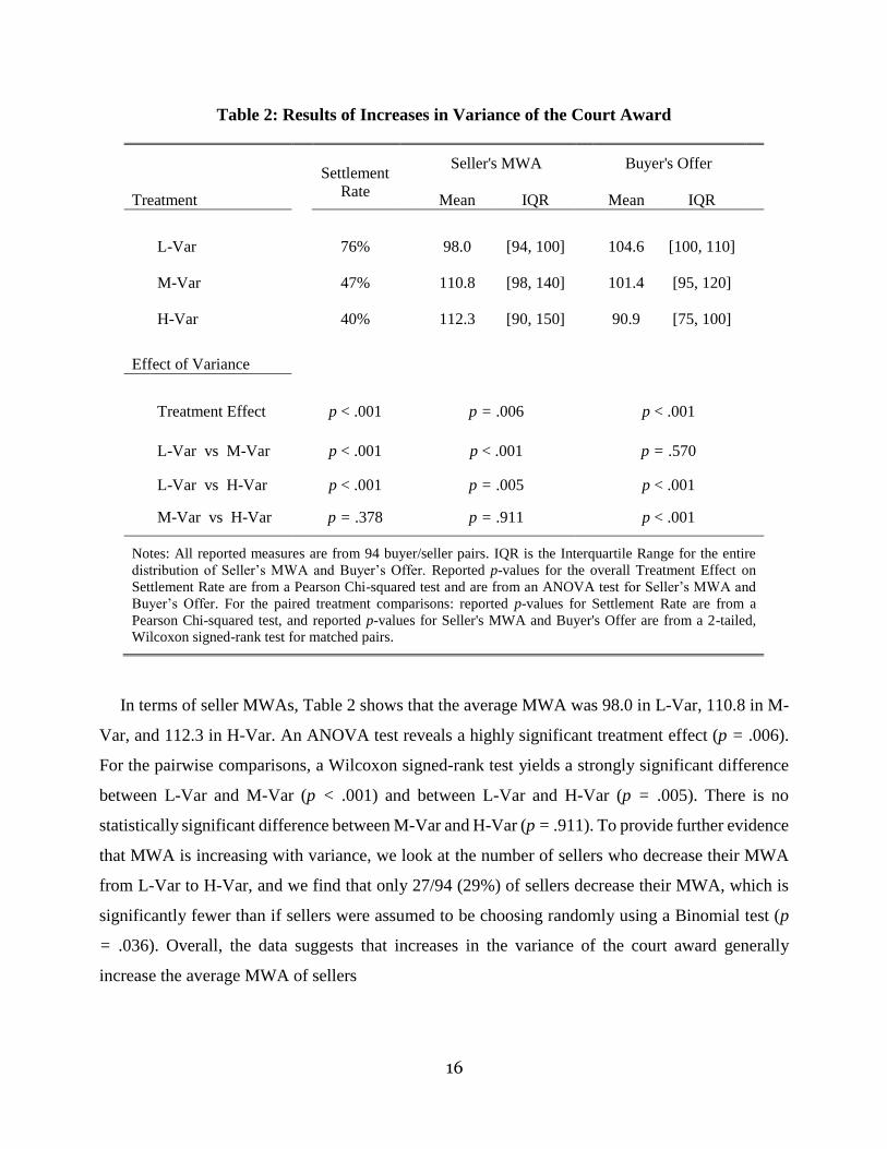
Looking first at the effect of increases in variance of the court award on settlement rates, we see
from column 1 of Table 2 that settlement rates were 76% in L-Var, 47% in M-Var, and 40% in H-
Var. A Pearson Chi-squared test yields a significant difference in settlement rates across the three
variance treatments (p < .001), indicating an overall treatment effect. Pairwise, the difference in
settlement rates between L-Var and M-Var and L-Var and H-Var are highly significant (p < .001; p
< .001; respectively), while the difference between M-Var and H-Var is not significant (p = .378).
Given the observed decrease in the settlement rates as variance increases, we next look at how the
increase in variance separately impacts seller and buyer behavior. The reduction in settlement rates
could be a result of sellers increasing their MWA, buyers reducing their offers, or both.
Var treatment there was a small difference at the 10% level with p = .083). We similarly tested for differences in buyer
offers across the two subject pools, and in none of the five treatments was there a significant difference at the 10% level. 27 We pool the three different sequencing versions. We tested for possible order effects by considering the pairwise
comparison of both seller MWAs and buyer offers for each of the three versions, for each of the five different treatments.
Of the 5 X 3 X 2 = 30 total pairwise comparisons, only 2 were significant at the 5% level, and 1 additional was significant
at the 10% level. For robustness, we also tested for overall differences in either seller MWAs or buyer offers between
the three versions, across the five different treatments, using a one-way ANOVA. Of the 5 X 2 =10 tests, only 1 was
significant at the 5% level. Overall, we feel this is within an acceptable threshold to assume no concerning order effects
and, consequently, pool the data in the analysis to provide a larger sample size and additional power.
16
Table 2: Results of Increases in Variance of the Court Award
Treatment
Settlement
Rate
Seller's MWA
Buyer's Offer
Mean IQR
Mean IQR
L-Var
76% 98.0 [94, 100]
104.6 [100, 110]
M-Var
47% 110.8 [98, 140]
101.4 [95, 120]
H-Var
40% 112.3 [90, 150]
90.9 [75, 100]
Effect of Variance
Treatment Effect p < .001 p = .006
p < .001
L-Var vs M-Var
p < .001 p < .001
p = .570
L-Var vs H-Var p < .001 p = .005 p < .001
M-Var vs H-Var
p = .378 p = .911
p < .001
Notes: All reported measures are from 94 buyer/seller pairs. IQR is the Interquartile Range for the entire
distribution of Seller’s MWA and Buyer’s Offer. Reported p-values for the overall Treatment Effect on
Settlement Rate are from a Pearson Chi-squared test and are from an ANOVA test for Seller’s MWA and
Buyer’s Offer. For the paired treatment comparisons: reported p-values for Settlement Rate are from a
Pearson Chi-squared test, and reported p-values for Seller's MWA and Buyer's Offer are from a 2-tailed,
Wilcoxon signed-rank test for matched pairs.
In terms of seller MWAs, Table 2 shows that the average MWA was 98.0 in L-Var, 110.8 in M-
Var, and 112.3 in H-Var. An ANOVA test reveals a highly significant treatment effect (p = .006).
For the pairwise comparisons, a Wilcoxon signed-rank test yields a strongly significant difference
between L-Var and M-Var (p < .001) and between L-Var and H-Var (p = .005). There is no
statistically significant difference between M-Var and H-Var (p = .911). To provide further evidence
that MWA is increasing with variance, we look at the number of sellers who decrease their MWA
from L-Var to H-Var, and we find that only 27/94 (29%) of sellers decrease their MWA, which is
significantly fewer than if sellers were assumed to be choosing randomly using a Binomial test (p
= .036). Overall, the data suggests that increases in the variance of the court award generally
increase the average MWA of sellers

17
Turning our attention to the behavior of the buyers, Table 2 reveals that buyers generally decrease
their offer as the court award becomes more variable. In particular, the average offer for buyers was
104.6 in L-Var, 101.4 in M-Var, and 90.9 in H-Var. An ANOVA test reveals an overall difference
across the three variance treatments (p < .001). For the pairwise comparisons, a Wilcoxon signed-
rank test does not reveal a significant difference between L-Var and M-Var (p = .570), but there is
a significant difference between L-Var and H-Var (p < .001) and between M-Var and H-Var (p <
.001). As further evidence that buyers are generally decreasing their offers as variance increases, we
find that only 19/94 (20%) buyers increase their offers from L-Var to H-Var, which a Binomial test
reveals is significantly fewer than if buyers were assumed to be choosing randomly (p < .001).
To better understand why settlement rates decreases as the variance increases, it is instructive to
examine the distributions of seller MWAs and buyer offers. We present this information in two
ways. First, in Table 2, we report the interquartile range (IQR) of the distribution of MWAs and
offers across the three variance treatments. Looking across the treatments, it is clear that the
distribution of MWAs becomes more dispersed with more mass moving to larger values (the range
of the IQR increases), as the variance of the court award increases. For buyers, as the variance
increases, the IQR of offers also increases, but more mass moves to smaller values. A settlement
occurs when the buyer’s offer is greater than or equal to the seller’s MWA; thus, for a randomly
matched pair of offer and MWA, the reported pattern in the IQRs suggest a decrease in the likelihood
of a settlement as the variance of the court award increases, which is consistent with the reported
settlement rates. This increase in dispersion becomes even clearer when we look at the distributions
of MWAs and offers. Figure 2 plots the histograms of MWAs and corresponding offers by treatment
(MWAs in the first row and offers below in the second row). From this picture, it is clear that the
underlying changes in the distribution of seller MWAs and buyer offers across the variance
treatments should, on average, lead to a reduction in settlement as variance increases.
The main results on the aggregate impact of increases in variance are summarized below:
Result 1a: Increases in the variance of the court award lead to lower settlement rates.
Result 1b: Increases in the variance of the court award generally increase seller MWAs.
Result 1c: Increases in the variance of the court award generally decrease buyer offers.

18
Taken together, these aggregate results suggest that increases in variance of the court award can
significantly impact negotiation behavior and, subsequently, settlement rates.
Figure 2: Distribution of Seller MWAs and Buyer Offers across Variance Treatments
3.1.2 The Effect of Increases in Skewness of the Court Award
To test the effects of increases in skewness of the court award, we compare the data from L-
Skew, M-Skew, and H-Skew; the distributions in all three treatments have the same mean and
variance, but the skewness increases from 0 to 3.14 to 7.87, respectively. Table 3 compares the
aggregate data for settlement rates, seller MWAs, and buyer offers.
Again, we first look at the effect of increases in skewness on settlement rates. From column 1 of
Table 3, we see that settlement rates were 40% in L-Skew, 60% in M-Skew, and 52% in H-Skew.
Comparing across the three skewness treatments, a Pearson Chi-squared test yields a significant
difference in settlement rates (p = .030). The pairwise difference between L-Skew and M-Skew is
significant (p = .009) and the difference between L-Skew and H-Skew is narrowly insignificant (p
= .108), while the difference between M-Skew and H-Skew is not significant (p = .304). Overall,

19
there appears to be a generally increasing relation between the skewness of the court award and
settlement rates. In particular, the settlement rate significantly increases when the court award
distribution transitions from zero skewness in the L-Skew treatment to being positively skewed in
the M-Skew and H-Skew treatments. To better understand these changes in settlement rates, we next
look the MWAs of sellers and the offers of buyers.
Table 3: Results of Increases in Skewness of the Court Award
Treatment
Settlement
Rate
Seller's MWA
Buyer's Offer
Mean IQR
Mean IQR
L-Skew 40% 112.3 [90, 150] 90.9 [75, 100]
M-Skew 60% 108.8 [70, 120] 97.6 [85, 110]
H-Skew 52% 138.5 [80, 131] 95.6 [90, 100]
Effect of Skewness
Treatment Effect
p = .030 p = .053
p = .174
L-Skew vs M-Skew
p = .009 p = .023
p = .020
L-Skew vs H-Skew
p = .108 p = .755
p = .400
M-Skew vs H-Skew
p = .304 p = .017
p = .504
Notes: All reported measures are from 94 buyer/seller pairs. IQR represents the Interquartile Range for the
entire distribution of Seller’s MWA and Buyer’s Offer. Reported p-values for the overall Treatment Effect
on Settlement Rate are from a Pearson Chi-squared test and are from an ANOVA test for Seller’s MWA and
Buyer’s Offer. For the paired treatment comparisons: reported p-values for Settlement Rate are from a
Pearson Chi-squared test, and reported p-values for Seller's MWA and Buyer's Offer are from a 2-tailed,
Wilcoxon signed-rank test for matched pairs.
For sellers, Table 3 shows that the average MWA was 112.3 in L-Skew, 108.8 in M-Skew, and
138.5 in H-Skew. An ANOVA test reveals a significant main effect of skewness on MWA (p =
.053). More specifically, a Wilcoxon signed-rank test reveals a significant difference between L-
Skew and M-Skew (p = .023) and between M-Skew and H-Skew (p = .017), while the difference
between the L-Skew and H-Skew is not statistically significant (p = .755). Overall, increases in
skewness seem to result in a non-monotonic effect on the MWA of sellers; the introduction of a

20
small initial increase in skewness (L-Skew to M-Skew) decreases MWAs, while a larger increase
in skewness (M-Skew to H-Skew) increases MWAs.
Proceeding next to buyers, Table 3 displays that the average offer was 90.9 in L-Skew, 97.6 in
M-Skew, and 95.7 in H-Skew. An ANOVA test does not reveal a significant difference in offers
across the three skewness treatments (p = .174). However, a Wilcoxon signed-rank test does result
in a significant pairwise difference between L-Skew and M-Skew (p = .020), while the difference
between L-Skew and H-Skew and M-Skew and H-Skew are not statistically significant (p = .400;
p = .504; respectively). Overall, increases in the skewness of the award distribution appear to have
a relatively small impact on buyer offers; the small impact is in the direction of buyers increasing
their offers as skewness increases (especially from L-Skew to M-Skew).
As before, the means of the distributions of seller MWAs and buyer offers do not fully capture
how increases in skewness of the award impact MWAs and offers. To get a better sense of why we
see the observed changes in settlement rates as skewness increases, we further examine the
distributions of seller MWAs and buyer offers. We report the corresponding interquartile ranges
(IQR) in Table 3 and the entire distributions in Figure 3 (MWAs in the first row and offers below
in the second row). Looking first at sellers, when skewness is introduced to the court award (moving
from L-Skew to M-Skew and H-Skew) two things seem to happen: (i) more mass from the middle
of the distribution of MWAs is shifted left to lower values (as evident by the IQR shifting left in M-
Skew and H-Skew compared to L-Skew), and (ii) more mass is simultaneously shifted right to very
large, outlying values (as evident by the MWA distributions in Figure 3), especially in H-Skew.28
For buyers, there is a moderate rightward shift in the distribution to higher offers moving from L-
Skew to M-Skew and, to a lesser extent, to H-Skew (as evident by the right shift in IQR). As a result
of these changes in the distributions of MWAs and offers as skewness increases, the increase in
settlement rates from L-Skew to M-Skew is driven by MWAs and offers being generally more
concentrated in the range of 80-120; as a result, for a randomly drawn buyer and seller, this should,
in expectation, lead to an increase in the probability of a settlement, as a larger portion of the
distributions overlap. A similar pattern emerges when comparing MWAs and offers between L-
28 A plausible contributing explanation of why mass is shifted to very high MWAs in the M-Skew and especially
the H-Skew treatments is longshot bias, where some sellers subjectively over-weight the likelihood of receiving the
very large, but unlikely, payoffs of 500 ECUs and 1000 ECUs. The presence of longshot bias has been documented
empirically (e.g., Camerer, 1989; Woodland & Woodland, 1994; 1999; Sobel & Raines, 2003; and Smith et al., 2006).

21
Skew and H-Skew, which generates the moderate increase in settlement rates in H-Skew compared
to L-Skew, despite the fact that average MWA actually increases in the H-Skew treatment.
Figure 3: Distribution of Seller MWAs and Buyer Offers across Skewness Treatments
The main results on the impact of increases in skewness of the court award, via the introduction
of low probability large awards in the distribution, are summarized below:
Result 2a: Increases in the skewness of the court award generally increase settlement rates.
Settlement rates initially increase as the award distribution becomes positively skewed, but then
flatten out as the distribution becomes more positively skewed.
Result 2b: Increases in the skewness of the court award have a non-monotonic effect on seller
MWAs. An initial increase in skewness (from no skewness) decreases MWAs, while a large
increases in skewness (from M-Skew to H-Skew) increase MWAs.
Result 2c: Increases in the skewness of the court award, at most, marginally increase buyer offers.
Overall, these aggregate results suggest that increases in the skewness of the court award can
significantly impact negotiation behavior and, subsequently, settlement rates.

22
3.3 Elicited Risk Preferences and Behavior in the ED Bargaining Task
To better understand how variance and skewness of the court award can possibly impact
negotiation behavior and settlement rates, we next consider the possible relation between elicited
risk preference measures and observed negotiation behavior. Before presenting these results, we
first present the descriptive statistics of the three different risk preference measures: (i) ES-risk, (ii)
HL-risk, and (iii) ES-prudence (see Section 2.2).29 The average of the ES-risk measure (total number
of the 10 lottery pairs where the individual chose the less risky option) across all the experimental
subjects was 7.70/10. The average HL-risk measure (the switching point to the more risky lottery)
was 6.33 for the 144 participants that had a unique switch point. The ES-risk and HL-risk are
significantly positively correlated, with a Spearman correlation coefficient of .478 (p < .001).
Because of the inability to recover a measure of risk aversion for all subjects using the HL-risk
measure, all the data analysis regarding risk aversion is performed using the ES-risk measure; for
robustness, all analyses are replicated using the HL-risk measure, and any qualitative differences
are reported. The average of the ES-prudence measure (total number of the 10 lottery pairs where
the individual chose the more prudent option) was 5.35/10.30
To explore the relation between risk measures and behavior in the ED task, we first stratify
subjects based on their elicited risk measures in the lottery task. A subject whose ES-risk measure
is above the median is classified as relatively risk-averse and below the median as relatively risk-
loving (likewise for the HL-risk measure). Similarly, a subject whose ES-prudence measure is above
the median is classified as relatively prudent and below the median as relatively imprudent.31
Henceforth, we drop the relative qualifier, but it is implied throughout the remainder of the analysis
29 We note that there were no significant differences in any of the three risk preference measures between the buyers
and the sellers in our study. Therefore, the role assignment in the ED bargaining task appears to have had a negligible
influence, if any, on the decisions made in the subsequent lottery task. 30 We document less prudent behavior than in previous studies. However, the absolute level of exhibited prudent
behavior is of less importance in our analysis since we explore how negotiation behavior of relatively more prudent
subjects compares with that of relatively more imprudent subjects. We postulate that the less prudent decisions observed
in our elicitation, relative to the previous studies, are a result of the fact that we represented the lottery choices in reduced
form rather than compound form. Therefore, we would caution readers from interpreting the prudence results as
providing evidence in contradiction to previous studies, which do find stronger evidence of more prudent behavior. 31 The relative stratification of risk preferences based on the median helps mitigate any possible order effects arising
from the lottery task following the ED task, which may have systematically led to either more or less risk-averse/prudent
lottery choices across all experimental participants. In addition this stratification generates a balanced sample. All of
the results are qualitatively robust if we instead classify subjects’ degree of risk aversion on an absolute scale, where
subjects whose HL-risk measure is 5 or less are classified as risk loving, and more than 5 are classified as risk averse.
23
that these risk preference characterizations are relative to the stratification of our participant sample
around the median value.
In the variance treatments, we expect risk-averse sellers to have lower MWAs than risk-loving
sellers. Furthermore, as the variance of the award increases, we expect the MWA of the relatively
more risk-averse subjects to decrease, and this effect should be stronger as compared to the more
risk-loving subjects. Conditional on the award distribution, we expect higher settlement rates
amongst risk-averse sellers due to their lower expected MWA. In the skewness treatments, we
expect prudent sellers to have higher MWAs in the M-Skew and H-Skew treatments than imprudent
sellers. As the skewness of the award increases, increases in MWA of more prudent subjects should
be relatively greater than those of the less prudent sellers. That said, we expect to see lower
settlement rates when the seller is more prudent because of the higher expected MWA.
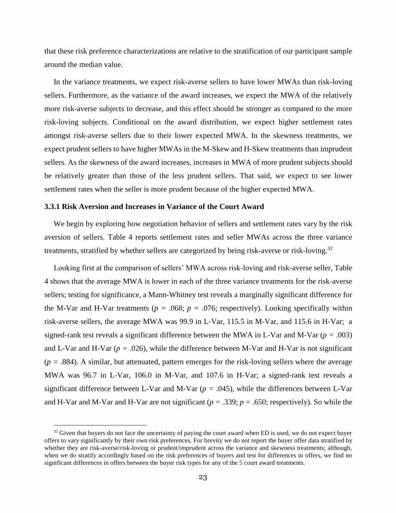
3.3.1 Risk Aversion and Increases in Variance of the Court Award
We begin by exploring how negotiation behavior of sellers and settlement rates vary by the risk
aversion of sellers. Table 4 reports settlement rates and seller MWAs across the three variance
treatments, stratified by whether sellers are categorized by being risk-averse or risk-loving.32
Looking first at the comparison of sellers’ MWA across risk-loving and risk-averse seller, Table
4 shows that the average MWA is lower in each of the three variance treatments for the risk-averse
sellers; testing for significance, a Mann-Whitney test reveals a marginally significant difference for
the M-Var and H-Var treatments (p = .068; p = .076; respectively). Looking specifically within
risk-averse sellers, the average MWA was 99.9 in L-Var, 115.5 in M-Var, and 115.6 in H-Var; a
signed-rank test reveals a significant difference between the MWA in L-Var and M-Var (p = .003)
and L-Var and H-Var (p = .026), while the difference between M-Var and H-Var is not significant
(p = .884). A similar, but attenuated, pattern emerges for the risk-loving sellers where the average
MWA was 96.7 in L-Var, 106.0 in M-Var, and 107.6 in H-Var; a signed-rank test reveals a
significant difference between L-Var and M-Var (p = .045), while the differences between L-Var
and H-Var and M-Var and H-Var are not significant (p = .339; p = .650; respectively). So while the
32 Given that buyers do not face the uncertainty of paying the court award when ED is used, we do not expect buyer
offers to vary significantly by their own risk preferences. For brevity we do not report the buyer offer data stratified by
whether they are risk-averse/risk-loving or prudent/imprudent across the variance and skewness treatments; although,
when we do stratify accordingly based on the risk preferences of buyers and test for differences in offers, we find no
significant differences in offers between the buyer risk types for any of the 5 court award treatments.

24
MWA tends to be lower for risk-averse sellers, there exists a similar positive relation between the
variance of the court award and the MWA for both risk-loving and risk-averse sellers.
Table 4: Stratification based on Risk Aversion of the Seller
Settlement Rates Seller’s MWA
Treatment
Risk
Loving
Risk
Averse p-value
Risk
Loving
Risk
Averse p-value
L-Var 77% 77% p = .961 99.9 96.7 p = .183
M-Var 49% 52% p = .810 115.5 106.0 p = .068
H-Var 33% 42% p = .459 115.5 107.6 p = .076
Effect of Variance
L-Var vs M-Var p = .010 p = .034 p = .003 p = .045
L-Var vs H-Var p < .001 p = .004 p = .026 p = .339
M-Var vs H-Var p = .167 p = .445 p = .844 p = .650
Notes: All reported measures are treatment-level averages stratified by whether the seller in the negotiating pair is classified
as relatively risk-averse (31 total pairs) or risk-loving (39 total pairs). For comparisons across risk-averse and risk-loving
subsamples, reported p-values are from a 2-tailed Mann-Whitney test. For the pairwise treatment comparisons: reported p-
values for Settlement Rate are from a Pearson Chi-squared test, and reported p-values for Seller's MWA are from a 2-tailed,
Wilcoxon signed-rank test for matched samples.
In terms of settlement rates, Table 4 displays that in all three variance treatments, settlement rates
tended to be higher whenever the seller was risk-averse, compared risk-loving, because of their
marginally lower MWA (on average); although, none of these differences are statistically
significant. Comparing settlement rates within seller types, for risk-loving sellers a Pearson Chi-
squared test across all three variance treatments reveals a significant difference (p < .001); in terms
of pairwise comparisons, the difference in settlement rate between L-Var and M-Var and L-Var and
H-Var are significant (p = .010; p < .001; respectively), while the difference between M-Var and
H-Var is not significant (p = .167). A very similar pattern of settlement rates emerges for risk-averse
sellers, where a Pearson Chi-squared test reveals a significant difference across the three variance
treatments (p = .014); the difference between L-Var and M-Var and L-Var and H-Var are significant
(p = .034; p = .004; respectively), while the difference between M-Var and H-Var is not significant
(p = .445). The data suggests that, conditional on the variance treatment, settlement rates are, at

25
most, marginally higher when negotiating with a more risk-averse seller. Furthermore, for both risk-
loving and risk-averse sellers, the data reveals a strong negative relation between settlement rates
and the variance of the court award.
Lastly, because prudence levels can impact how people makes choices under the presence of
background risk, we also look at whether seller MWAs react differently to increases in variance of
the court award based on their degree of prudence. For sellers classified as imprudent, their average
MWA was 97.4 in L-Var, 114.1 in M-Var, and 109.3 in H-Var. For sellers classified as prudent,
their average MWA was 97.3 in L-Var, 106.1 in M-Var and 112.2 in H-Var. Comparing across
prudent and imprudent sellers, the difference in MWA is not significant for any of the three variance
treatments using a Mann-Whitney test (p = .376; p = .261; p = .821; respectively). Moreover, for
both prudent and imprudent sellers we see the same general pattern of MWAs increasing as the
variance of the award distribution increases from the L-Var treatment to the M-Var and H-Var
treatments. As such, it does not appear that our aggregate results regarding how sellers react to
increases in variance of the court award, and the consequent effect on settlement rates, are being
driven by differential reactions to the increase in variance between prudent and imprudent sellers.
The main results on the observed relation between increases in variance of the court award and
individual measures of risk aversion are summarized as follows:
Result 3a: Risk-averse sellers have marginally lower MWAs, but increases in variance of the court
award generally increase the MWA for both risk-averse and risk-loving sellers.
Result 3b: Settlement rates are marginally higher when sellers are risk-averse, but there is a strong
negative relation between settlement rates and variance of the court award for risk-averse and risk-
loving sellers.
3.3.2 Prudence and Increases in Skewness of the Court Award
Next, we explore if and to what extent negotiation behavior and settlement rates vary by the
prudence of sellers as the skewness of the court award increases. Table 5 shows settlement rates and
seller MWAs for the three skewness treatments stratified by imprudent and prudent sellers.
Looking first that the MWA of sellers, the right two columns of Table 5 reports the average
MWA across the three skewness treatments for both imprudent and prudent sellers. For the
imprudent sellers, the average MWA was 109.3 in L-Skew, 107.0 in M-Skew, and 141.2 in H-Var,

26
while the corresponding average MWA for prudent sellers was 112.2, 114.2, and 139.6,
respectively. Comparing across prudent and imprudent sellers, the average MWA is generally very
similar the L-Skew, M-Skew and H-Skew treatments, and none of the differences are statistically
significant using a Mann-Whitney test (p = .410; p = .441; p = .420; respectively).33 Within seller
type, for imprudent sellers there are no significant differences in MWA across the three skewness
conditions; while the average MWA in the H-skew condition appears to be much larger than in the
L-Skew and M-skew, this is being driven by a few outliers reporting very high MWAs in the H-
Skew treatment. Looking next within prudent sellers, there are no significant differences in MWA
between L-Skew and M-Skew or L-Skew and H-Skew, but the difference between M-Skew and H-
Skew is marginally significant using a signed-rank test (p = .074). Overall, the data reported in
Table 5 reveals that, conditional on the skewness of the court award, the sellers’ MWA is similar
between sellers classified as being prudent and imprudent, and prudent sellers are marginally more
responsive – their MWA marginally increases – as the court award becomes highly skewed in the
H-Skew treatment.
In terms of settlement rates, the left two columns of Table 5 report the settlement rates across
imprudent and prudent sellers for the L-Skew, M-Skew and H-Skew treatments. Comparing across
imprudent and prudent sellers, the settlement rates are similar in the L-Skew treatment (38% and
42% respectively), and are slightly higher for prudent sellers in M-Skew treatment (64% compared
to 50%) and in the H-Skew treatment (57% compared to 45%); however, these settlement rates are
not statistically significant using a Pearson Chi-squared test (p = .621; p = .191; p = .272;
respectively). At first glance, the fact that settlement rates are higher for the set of prudent sellers
seems contradictory given that the average MWA is higher for prudent sellers. However, what is
driving the higher settlement rates for the group of prudent sellers is a change in the shape of the
distribution of MWAs. In particular, the median offer is actually lower for the prudent sellers
compared to imprudent sellers in both M-Skew (90 compared to 100) and H-Skew (97.5 compared
33 We would expect prudent sellers, who have a preference for positive skewness, to express higher WTA, on
average, in the M-Skew and H-Skew treatments. One plausible reason why we did not observe such a pattern in our
data is that our participant sample, in the aggregate, exhibited a relatively low degree of prudence in the lotter elicitation
task – only choosing the more prudent option an average of 5.35/10 and a median of 5/10. Thus, many of the sellers
classified as relatively prudent (above the median) may not have been overly prudent. In addition, of the 42 sellers
classified as prudent, 15 were also classified in the domain of being relatively risk-loving; these risk-loving sellers could
have expressed a higher WTP in the M-Skew and H-Skew treatments in response to the possible misperception that
those court award distributions had more variance.

27
to 100). Thus, for prudent sellers more mass is shifting to lower MWAs in the M-Skew and H-skew
treatments (despite the fact that the average MWA is increasing), which then makes it more likely
that the buyer’s offer will be higher than the seller’s MWA and a settlement will occur. In terms of
settlement rates within seller type and across the skewness treatments, a very similar pattern emerges
for both prudent and imprudent sellers; namely, settlement rates increase from L-Skew to M-Skew
and then slight decrease from M-Skew to H-skew. Overall, the data suggests that settlement rates
are similar whether negotiating with a prudent or imprudent seller.
Table 5: Stratification based on Prudence of the Seller
Settlement Rates Seller’s MWA
Treatment Imprudent Prudent p-value Imprudent Prudent p-value
L-Skew 38% 42% p = .621 109.3 112.2 p = .410
M-Skew 50% 64% p = .191 107.0 114.2 p = .441
H-Skew 45% 57% p = .272 141.2 139.6 p = .420
Effect of Variance
L-Skew vs M-Skew p = .260 p = .049 p = .269 p = .257
L-Skew vs H-Skew p = .496 p = .190 p = .973 p = .462
M-Skew vs H-Skew
p = .654 p = .503 p = .384 p = .074
Notes: All reported measures are treatment-level averages stratified by whether the seller in the negotiating pair is classified
as relatively imprudent (40 total pairs) or prudent (42 total pairs). For comparisons across imprudent and prudent subsamples,
reported p-values are from a 2-tailed Mann-Whitney test. For the pairwise treatment comparisons: reported p-values for
Settlement Rate are from a Pearson Chi-squared test, and reported p-values for Seller's MWA are from a 2-tailed, Wilcoxon
signed-rank test for matched samples.
Lastly, we consider if seller MWAs possibly react differently to increases in skewness of the
court award based on their degree of risk aversion. For those sellers classified as risk-loving, their
average MWA was 115.5 in L-Skew, 118.1 in M-Skew, and 162.6 in H-Skew. For sellers classified
as risk-averse, their average MWA was 107.6 in L-Skew, 110.4 in M-Skew and 125.2 in H-Skew.
While the average MWA is higher for the risk-loving sellers in all three skewness treatments, a
Mann-Whitney test does not reveal a statistically significant difference for any of the three
treatments (p = .151; p = .252; p = .301; respectively). What appears to be a large difference in the

28
average MWA in the H-Skew treatment is driven primarily by a few risk-loving outliers expressing
very large MWAs.34 Thus, risk-averse sellers appear to be expressing, at most, marginally higher
MWAs as the skewness of the court award increases.
The main results regarding the relationship between prudence of the seller and outcomes in the
ED negotiations as the court award becomes more skewed are summarized as follows:
Result 4a: The average MWA for prudent and imprudent sellers is similar, but only the prudent
sellers tend to increase their MWA as the court award becomes highly skewed
Result 4a: Overall, settlement rates are marginally higher for prudent sellers compared to imprudent
sellers, but settlement rates for both prudent and imprudent sellers exhibit a similar pattern as the
skewness of the court award increases.
3.4 Welfare implication of Increases in Variance and Skewness
We conclude the results section by discussing the welfare implications of our findings. In doing
so, it is important to note that decreases in settlement rates are not necessarily evidence of more
inefficiency. The reason being is that, given the fixed payment of 50 ECUs for the buyer when there
is a settlement failure, the buyer would never offer more than 150 ECUs to settle (as he would be
better off litigating); as a result, settlement failure is only inefficient in instances when the seller’s
MWA is less than 150 ECUs. When the seller’s MWA is less than 150 ECUs the contact zone,
which refers to the range of prices that are higher than the seller’s MWA (i.e., the seller’s
reservation) and lower than 150 ECUs (i.e., the buyer’s reservation), is non-empty and there is the
possibility, ex-ante, for the buyer and seller to reach an efficient settlement.
In order to better ascertain the welfare effect of increases in variance and skewness of the court
award, we look at the number of potentially efficient settlements that were actually reached, where
a potentially efficient settlement is defined as an instance where the seller’s MWA was less than or
equal to 150 ECUs. Table 6 presents the fraction of sellers with a MWA less than or equal to 150
ECUs, and the number of potentially efficient settlements reached for each treatment. Looking first
at the two rightmost columns of Panel A, we see that as the variance increases, the number of
34 Chiu (2005) document that agents may prefer more variable distributions if they are also more skewed. Hence,
some risk-averse sellers may have been operating as if there were a tradeoff between variance and skewness, and may
have had a higher MWA for the H-Skew distribution, which they erroneously perceived as being more variable that the
L-Skew and M-Skew distributions.

29
potentially efficient settlements reached monotonically decreases from 75.6% (L-Var) to 51.1% (M-
Var) to 46.3% (H-Var). A Pearson Chi-squared test across all three variance treatments reveals a
significant difference (p < .001); moreover, the difference in settlement rates between L-Var and
M-Var and L-Var and H-Var are significant (p = .001; p < .001; respectively), while the difference
between M-Var and H-Var is not significant (p = .532).
Table 6: Comparison of Potentially Efficient Settlements Reached by Treatment
Panel A: The Effect of Increasing Variance
Seller’s MWA < 150 ECUs # of Potentially Efficient
Settlements Reached
Treatment Fraction Percent Fraction Percent
L-Var 94/94 100% 71/94 75.6%
M-Var 86/94 91.5% 44/86 51.1%
H-Var 82/94 87.2% 38/82 46.3%
Panel B: The Effect of Increasing Skewness
Seller’s MWA < 150 ECUs
# of Potentially Efficient
Settlements Reached
Treatment Fraction Percent Fraction Percent
L-Skew 82/94 87.2% 38/82 46.3%
M-Skew 83/94 88.3% 56/83 67.5%
H-Skew 80/94 85.1% 49/80 61.3%
In terms of how increases in skewness impact efficient settlements, the two rightmost columns
of Panel B in Table 6 display the fraction of potentially efficient settlements reached across the three
skewness treatments is 46.3% in H-Skew, 67.5% in M-Skew, and 61.3% in H-Skew. A Pearson Chi-
squared test across all three skewness treatments reveals a significant difference (p = .018); in terms
of pairwise comparisons, the difference in settlement rates between L-Var and M-Var and L-Var
and H-Var are significant (p = .006; p = .057; respectively), while the difference between M-Var
and H-Var is not significant (p = .407).

30
Thus, from a welfare perspective, we see that there is significantly more inefficient litigation as
the variance of the court award increases. While there are fewer potentially efficient settlements as
variance increases, there are also relatively fewer settlements actually reached; this seems to be
driven in large part by more mass in the aggregate distribution of MWAs being shifted to higher
values (i.e., many sellers respond to the higher variance with a higher MWA), while more mass in
the aggregate distribution buyer offers is shifted to lower values. With regard to skewness, we see
that a moderate initial increase in skewness (from L-Skew to M-Skew) significantly decreases the
incidence of inefficient litigation, but this effect flattens out as skewness increases further (from M-
Skew to H-Skew). As the skewness increases from L-Skew to M-Skew, the number of potentially
efficient settlements stays relatively constant, but a significantly larger fraction of the potentially
efficient settlements actually settle. This reason for this is twofold: (i) buyers generally increase
their offers as the skewness increases, and (ii) more mass in the distribution of MWAs is shifted to
lower values (despite the presence of a few outliers at the very upper end of the MWA distribution
that pull the average MWA higher as the skewness increases).
4 Replication using Abstract Framing
In our baseline experimental design, we include a substantial degree of contextual framing in the
negotiation task (i.e., seller/buyer labeling, the description of land ownership, the ED legal context,
and the possible adjudicated court award). A potential concern is that our primary findings are, at
least partially, an artifact of the contextual framing interacting with the treatments; thus, limiting the
generalizability of our results.35
To investigate the role of possible framing effects in our study, we ran additional sessions at
Florida State University with a completely abstract framing with no mention of a legal environment
(a copy of the unframed experimental instructions is provided in Appendix C); henceforth, these
sessions are referred to as the unframed condition.36 In total, we ran 6 unframed sessions with a total
35 Given that testing for framing effects is not the primary motivation of our paper, we refrain from providing a
comprehensive review of the literature, which is rather extensive. Instead we refer readers to Abbink & Hennig-Schmidt
(2006) and Dufwenberg et al. (2011) and the references thein for more detailed discussion about framing effects, as well
as Copper et al. (1999), Stahl & Haruvy (2008), and Barr & Serra (2009) for experimental studies comparing behavior
under non-neutral and neutral framing. More specific to our setting, Babcock & Loewenstein (1997) discuss the benefits
of using a legal context in the framing of their study involving topics related to legal disputes. 36 Specifically, participants were given generic role labels of Player A (instead of buyer) and Player B (instead of
seller), their object of the negotiation was a token, and failure to reach an agreement would result in Player B (who was
originally endowed with the token) receiving a draw from a lottery of payouts (as opposed to a court award).
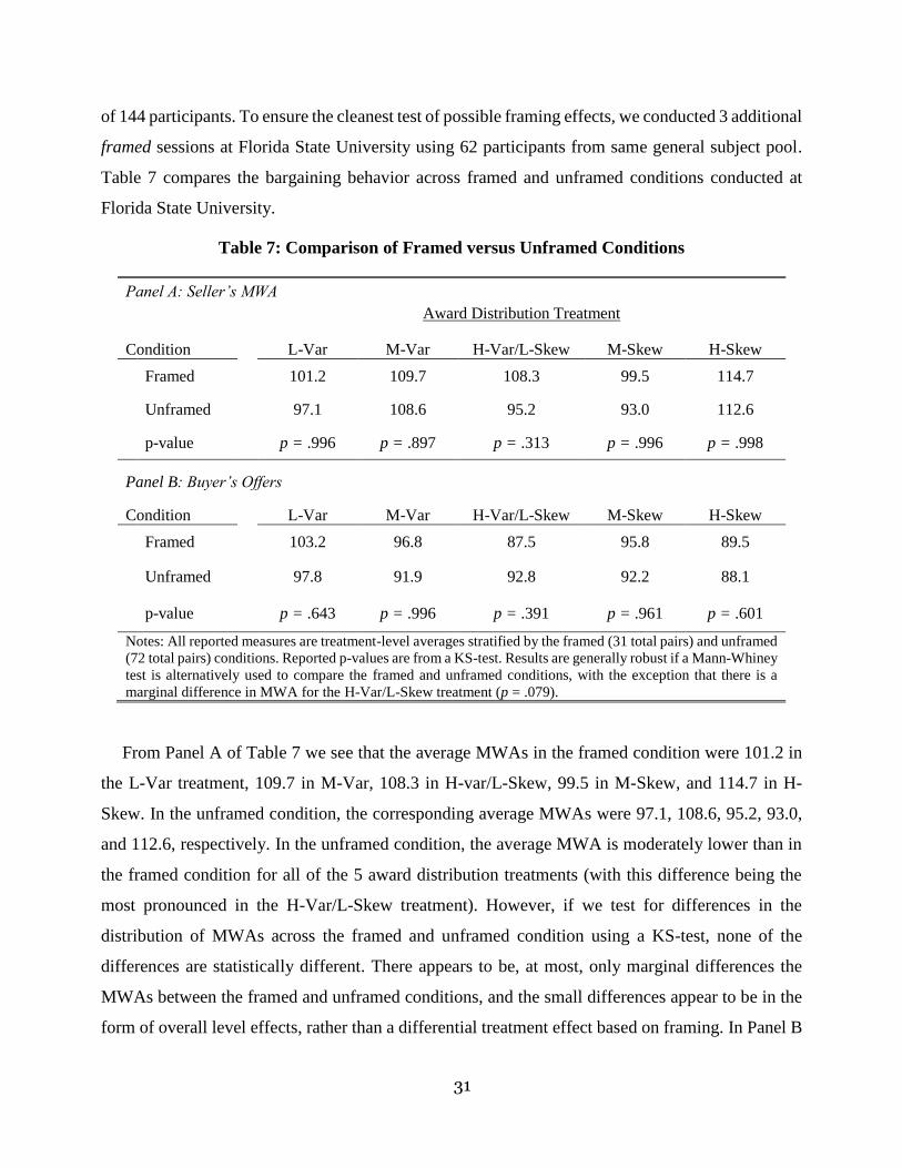
31
of 144 participants. To ensure the cleanest test of possible framing effects, we conducted 3 additional
framed sessions at Florida State University using 62 participants from same general subject pool.
Table 7 compares the bargaining behavior across framed and unframed conditions conducted at
Florida State University.
Table 7: Comparison of Framed versus Unframed Conditions
Panel A: Seller’s MWA
Award Distribution Treatment
Condition L-Var M-Var H-Var/L-Skew M-Skew H-Skew
Framed 101.2 109.7 108.3 99.5 114.7
Unframed 97.1 108.6 95.2 93.0 112.6
p-value p = .996 p = .897 p = .313 p = .996 p = .998
Panel B: Buyer’s Offers
Condition L-Var M-Var H-Var/L-Skew M-Skew H-Skew
Framed 103.2 96.8 87.5 95.8 89.5
Unframed 97.8 91.9 92.8 92.2 88.1
p-value p = .643 p = .996 p = .391 p = .961 p = .601
Notes: All reported measures are treatment-level averages stratified by the framed (31 total pairs) and unframed
(72 total pairs) conditions. Reported p-values are from a KS-test. Results are generally robust if a Mann-Whiney
test is alternatively used to compare the framed and unframed conditions, with the exception that there is a
marginal difference in MWA for the H-Var/L-Skew treatment (p = .079).
From Panel A of Table 7 we see that the average MWAs in the framed condition were 101.2 in
the L-Var treatment, 109.7 in M-Var, 108.3 in H-var/L-Skew, 99.5 in M-Skew, and 114.7 in H-
Skew. In the unframed condition, the corresponding average MWAs were 97.1, 108.6, 95.2, 93.0,
and 112.6, respectively. In the unframed condition, the average MWA is moderately lower than in
the framed condition for all of the 5 award distribution treatments (with this difference being the
most pronounced in the H-Var/L-Skew treatment). However, if we test for differences in the
distribution of MWAs across the framed and unframed condition using a KS-test, none of the
differences are statistically different. There appears to be, at most, only marginal differences the
MWAs between the framed and unframed conditions, and the small differences appear to be in the
form of overall level effects, rather than a differential treatment effect based on framing. In Panel B
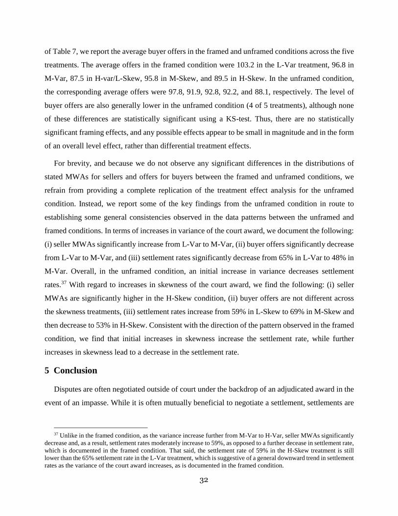
32
of Table 7, we report the average buyer offers in the framed and unframed conditions across the five
treatments. The average offers in the framed condition were 103.2 in the L-Var treatment, 96.8 in
M-Var, 87.5 in H-var/L-Skew, 95.8 in M-Skew, and 89.5 in H-Skew. In the unframed condition,
the corresponding average offers were 97.8, 91.9, 92.8, 92.2, and 88.1, respectively. The level of
buyer offers are also generally lower in the unframed condition (4 of 5 treatments), although none
of these differences are statistically significant using a KS-test. Thus, there are no statistically
significant framing effects, and any possible effects appear to be small in magnitude and in the form
of an overall level effect, rather than differential treatment effects.
For brevity, and because we do not observe any significant differences in the distributions of
stated MWAs for sellers and offers for buyers between the framed and unframed conditions, we
refrain from providing a complete replication of the treatment effect analysis for the unframed
condition. Instead, we report some of the key findings from the unframed condition in route to
establishing some general consistencies observed in the data patterns between the unframed and
framed conditions. In terms of increases in variance of the court award, we document the following:
(i) seller MWAs significantly increase from L-Var to M-Var, (ii) buyer offers significantly decrease
from L-Var to M-Var, and (iii) settlement rates significantly decrease from 65% in L-Var to 48% in
M-Var. Overall, in the unframed condition, an initial increase in variance decreases settlement
rates.37 With regard to increases in skewness of the court award, we find the following: (i) seller
MWAs are significantly higher in the H-Skew condition, (ii) buyer offers are not different across
the skewness treatments, (iii) settlement rates increase from 59% in L-Skew to 69% in M-Skew and
then decrease to 53% in H-Skew. Consistent with the direction of the pattern observed in the framed
condition, we find that initial increases in skewness increase the settlement rate, while further
increases in skewness lead to a decrease in the settlement rate.
5 Conclusion
Disputes are often negotiated outside of court under the backdrop of an adjudicated award in the
event of an impasse. While it is often mutually beneficial to negotiate a settlement, settlements are
37 Unlike in the framed condition, as the variance increase further from M-Var to H-Var, seller MWAs significantly
decrease and, as a result, settlement rates moderately increase to 59%, as opposed to a further decease in settlement rate,
which is documented in the framed condition. That said, the settlement rate of 59% in the H-Skew treatment is still
lower than the 65% settlement rate in the L-Var treatment, which is suggestive of a general downward trend in settlement
rates as the variance of the court award increases, as is documented in the framed condition.
33
not ubiquitous, and the involved parties are often resigned to the use of costly litigation.
Furthermore, the adjudicated award in such settings can be highly unpredictable and variable
(Sunstein et al., 2002). We contend that the presence of uncertainty in the adjudicated award can
impact settlement negotiation behavior and, consequently, the likelihood that a settlement is
reached. We investigate this hypothesis empirically using a laboratory experiment where we
systematically increase the variance and skewness of the award distribution across treatments. In
addition, we also elicit individual measures of risk aversion and prudence to test for heterogeneous
treatment effects based on risk attitudes. We view our results as being applicable to a variety of legal
disputes where adjudicated awards are likely to be uncertain including: punitive damages, patent
infringements, contract breaches, antitrust, labor disputes, and eminent domain.
Overall, our results suggest that court award uncertainty can significantly impact settlement
negotiations and, consequently, settlement rates. In particular, we find that increases in the variance
of the court award lead to lower settlement rates. This result is driven by sellers generally increasing
their minimum willingness to accept (MWA) as the variance of the award increases, while buyers
generally decrease their price offers. When we further examine the data, classifying sellers as
relatively risk-averse or risk-loving, we find a similar pattern for both types of sellers. Regarding
increases in skewness of the court award, we find that settlement rates generally increase, although
the increase is the strongest for an initial increase in skewness (from zero skewness to some positive
skewness in the distribution). This seems to be driven by seller MWAs being more concentrated at
lower values as skewness increases (despite the presence of skewness seeking outliers who express
very large MWAs, especially in the H-Skew treatment), while buyers moderately increase their price
offers. Notably, our main results are generally robust in both a contextually framed settlement
negotiation environment and an abstractly framed negotiation environment, which provides more
robust and convincing evidence that increases in variance and skewness of adjudicated awards can
impact settlement negotiation in significant and important ways.
It is worth noting that in our design, lottery complexity – the number of possible outcomes in the
lottery – varies across the five treatment. This may be relevant since it has been documented
experimentally that agents prefer less complex lotteries (See Huck & Weizsäcker, 1999; Mador et
al., 2000; and Sonsino et al., 2002). In the context of our design, the distribution in M-Var (5
outcomes) is more complex than the distributions in L-Var and H-Var (2 outcomes each). Likewise,
the distributions in M-Skew and H-Skew (6 and 5 outcomes, respectively) are more complex than

34
L-Skew (2 outcomes). Thus, based on the previous findings, some sellers in our experiment may
have been less attracted to the M-Var distribution (compared to L-Var), which should have lowered
their MWA. Similarly, some sellers may have been less attracted to the M-Skew and H-Skew
treatments (compared to L-Skew) and, hence, lowered their MWA. However, these effects generally
work in the opposite direction of our main findings. As a result, it seems unlikely that the difference
in lottery complexity across treatments substantially confounded our results.
An interesting pattern that emerges in our data is the positive relation between sellers’ MWA and
the variance of the court award; moreover, this positive relation holds even for those seller who are
risk-averse (especially when going from L-Var to M-Var), which seems counter-intuitive. While
not the primary motivation of the paper, we briefly speculative about a possible mechanism that
could be driving this pattern. In both the M-Var and H-Var treatments, there is the possibility for
sellers to receive much larger awards compared to the L-Var treatment. We suspect that these larger
awards might have been more salient to sellers (Bordalo et al., 2012; 2015), especially given the
contextual framing of the negotiation environment where the sellers become enticed with the
prospect of the court awarding them a large payout. As a result of sellers possibly being drawn to
these large and more salient awards, they may have subjectively over-weighted the likelihood of
receiving these larger awards leading to inflated MWAs.38
When examining welfare implications, we note that when court awards are uncertain, settlement
failure is not always necessarily inefficient. The reason is that when awards are highly variable or
largely positively skewed, the plaintiff’s reservation value to settle may be much larger than the
expected court award; this could result if the plaintiff has a strong preference for skewed award
distributions, exhibits long-shot bias or saliency bias, or becomes enticed with the possibility to “hit
it big”. If the plaintiff’s reservation value is too large, there may be no possibility for a mutually
agreeable settlement. In such instances, settlement failure is not inefficient, and we would expect
litigation to be imminent. This is apparent in our data where in the high variance (high skewness)
treatments, settlement is not efficient for 13 percent (15 percent) of the negotiating pairs, since the
38 The plausibility of saliency bias contributing to sellers stating higher MWAs in the M-Var and H-Var treatments
is reinforced when we look at the unframed condition. With completely abstract framing and no mention of court
awards, we would expect the large values of the distribution to be less salient to sellers, relative to the framed condition.
As such, the larger awards would receive less weight in the unframed conditions and sellers would respond with lower
MWAs, relative to the framed condition. While not statistically significant, the average MWAs in the H-Var condition
(where there is the presence of just one large award) is lower than in the framed condition, providing some indirect
evidence in-line with saliency bias playing a role.

35
seller’s MWA exceed the buyer’s expected payment of proceeding to court. However, even if we
restrict the analysis to the subset of disputes where an efficient settlement was possible, we see the
following results emerge. First, high levels of variance in the court award lead to an increase in
excessive, inefficient litigation. Second, some positive skewness in the court award leads to a
decrease in inefficient litigation. Importantly, our results show that court award uncertainty can
impact settlement rates through two channels: (i) by reducing the number of potentially efficient
settlements, and (ii) by altering the number of potentially efficient settlements that are actually
reached (i.e., the instance of inefficient litigation).
We note that the implications of our results would be applicable even in dispute settings where
the actual underlying court award had very little uncertainty; rather, the plaintiff had misguided
perceptions about the award distribution. This scenario could arise if, for example, the plaintiff held
an erroneous or biased belief regarding the magnitude of possible court awards, or the likelihood of
receiving awards at the upper end of the distribution. Such misguided beliefs could occur if plaintiffs
exhibit “self-serving” biases where they may over-estimate the value of the adjudicated award,
which has been documented (e.g., Loewenstein et al., 1993; Babcock et al., 1995; Babcock &
Loewenstein, 1997). In such a case, litigation may be the preferred course of action for the
defendant, as the defendant’s expected payoff may be lower than paying the requisite amount to
settle. While we do not explore asymmetries in beliefs about awards, this could be an interesting
area for future research.
While we believe our design contributes to our overall understanding of settlement failures in
legal disputes, we acknowledge the possible limitations of our study. Our sample is comprised of
student subjects who were randomly assigned their roles and who may be inexperienced, while legal
disputes usually involve expert lawyers who may be able to more accurately predict the responses
of a jury or a particular judge. Indeed, more experienced subjects may have been able to avoid court
with a higher frequency, resulting in less inefficient litigation, although this is purely speculative.
That said, plaintiffs who file suit may be inexperienced, and they are the ones ultimately deciding
whether to accept any proposed settlement offer. Another possible limitation is that participants only
partook in five rounds of the negotiation (one round for each different award distribution) and, thus,
had little opportunity to learn in this environment. Again we speculate that as the negotiating parties
learn through experience, we may observe attenuated effects of changes in variance and skewness
of adjudicated on settlement rates. At the same time, there is likely to be substantial heterogeneity

36
from one legal dispute to the next and litigants may only be occasionally involved in disputes, which
would minimize the opportunities for learning (as discussed by Babcock and Loewenstein, 1997).
In terms of broader implications, we recognize that explicitly manipulating the level of
uncertainty of adjudicated awards is likely not a plausible mechanism for reducing inefficient
litigation. Yet, the results from this study can provide useful insights as to other more feasible
approaches. For example, one approach would be to extend the use of award caps, which several
states have implemented through widespread tort reform over the past several decades. Such award
caps could have the effect of moderating the level of perceived variance and/or skewness in the
award distribution (in addition to possibly lowering the perceived mean); as a result, the
corresponding decrease in perceived variance and/or skewness could lead to higher efficient
settlement rates, even if the perceived mean award remains unchanged after the imposition of the
award cap.39 Another possible approach might be to institute measures that increase the quantity
and/or accuracy of information available to the plaintiff, such as the mandatory disclosure provision
of Rule 26 of the Federal Rules of Civil Procedure. Such mandates may reduce the variance in
plaintiffs’ assessment of the award distribution, which could reduce inefficient litigation.
39 Much of the prior literature on the effect of award caps on litigation has focused on how award caps can impact
the level of care taken by the liable party, or the likelihood that the potential claimant files a claim. We are by no means
suggesting that these types of moral hazard effects and selection effects are not possible consequences of award caps.
Rather, we are suggesting that another possible avenue through which award caps can impact litigation is by altering
the degree of award uncertainty and, subsequently, the likelihood that a settlement is reached.

37
References
1. Abbink, K., & Hennig-Schmidt, H. (2006). “Neutral versus loaded instructions in a bribery
experiment.” Experimental Economics 9, 103-121.
2. Anbarci, N., and Feltovich, N. (2013). “How sensitive are bargaining outcomes to changes in
disagreement payoffs?” Experimental Economics 16, 560-596.
3. Avraham, R. (2007). “An empirical study of the impact of tort reforms on medical malpractice
settlement payments.” The Journal of Legal Studies 36, 183-229.
4. Babcock, L., and Landeo, C. (2004). “Settlement escrows: an experimental study of a bilateral
bargaining game.” Journal of Economic Behavior & Organization 53, 401-417.
5. Babcock, L. and Loewenstein, G. (1997). “Explaining Bargaining Impasse: The Role of Self-Serving
Biases.” The Journal of Economic Perspectives 11, 109-126.
6. Babcock, L., Loewenstein, G., Issacharoff, S., & Camerer, C. (1995). “Biased judgments of fairness
in bargaining.” The American Economic Review 85, 1337-1343.
7. Babcock, L., and Pogarsky, G. (1999). “Damage caps and settlement: A behavioral approach.” The
Journal of Legal Studies 28, 341-370.
8. Barr, A., & Serra, D. (2009). “The effects of externalities and framing on bribery in a petty corruption
experiment.” Experimental Economics 12, 488-503.
9. Bebchuk, L. (1984). “Litigation and settlement under imperfect information.” The RAND Journal of
Economics 15, 404-415.
10. Black, B., Silver, C., Hyman, D., and Sage, W. (2005). “Stability, not crisis: Medical malpractice
claim outcomes in Texas, 1988-2002.” Journal of Empirical Legal Studies 2, 207-259.
11. Boles, T., Croson, R., and Murnighan, K. (2000). “Deception and retribution in repeated ultimatum
bargaining.” Organizational Behavior and Human Decision Processes 83, 235-259.
12. Bordalo, P., Gennaioli, N., and Shleifer, A. (2012). “Salience theory of choice under risk.” The
Quarterly Journal of Economics 127, 1243-1285.
13. Bordalo, P., Gennaioli, N., & Shleifer, A. (2015). “Salience Theory of Judicial Decisions.” The
Journal of Legal Studies 44, S7-S33.
14. Brandts, J., and Charness, G. (2011). “The strategy versus the direct-response method: a first survey
of experimental comparisons.” Experimental Economics 14, 375-398.
15. Brasch, W. (2013, May 19) Keystone XL, Through Transcanada, Uses Eminent Domain to Seize
Texan's Land. OpEdNews, 19 May 2013. Web. 26 Oct. 2013.
‹https://owl.english.purdue.edu/owl/resource/747/08/›.
16. Browne, M., and Puelz, R. (1999). “The effect of legal rules on the value of economic and non-
economic damages and the decision to file.” Journal of Risk and Uncertainty 18, 189-213.
17. Camerer, C. (1989). “Does the Basketball Market Believe in the Hot Hand?” The American
Economic Review 79, 1257-1261.
18. Charness, G., Gneezy, U., and Imas, A. (2013). “Experimental methods: Eliciting risk preferences.”
Journal of Economic Behavior and Organization 87, 43-51.
19. Chiu, H. (2005). “Skewness preference, risk aversion, and the precedence relations on stochastic
changes.” Management Science 51, 1816-1828.

38
20. Chu, C. Y., and Chien, H-K. (2007). “Asymmetric information, pretrial negotiation and optimal
decoupling.” International Review of Law and Economics 27, 312-329.
21. Collins, S. and Isaac, M. (2012). “Holdout: Existence, Information, and Contingent Contracting.”
Journal of Law and Economics 55, 793-814.
22. Cooper, D. J., Kagel, J. H., Lo, W., & Gu, Q. L. (1999). “Gaming against managers in incentive
systems: Experimental results with Chinese students and Chinese managers.” American Economic
Review 89, 781-804.
23. Cox, J., and Harrison, G. (2008). Risk Aversion in Experiments. New York: JAI Press.
24. Croson, R., Boles, T., amd Murnighan, K. (2003). “Cheap talk in bargaining experiments: lying and
threats in ultimatum games.” Journal of Economic Behavior & Organization 51, 143-159.
25. Croson, R., and Mnookin, R. (1997). “Does Disputing through Agents Enhance Cooperation-
Experimental Evidence.” Journal of Legal Studies 26, 331-345.
26. Dave, C., Eckel C., Johnson, C., and Rojas, C. (2010) “Eliciting risk preferences: When is simple
better?” Journal of Risk and Uncertainty 41, 219-243.
27. Deck, C., and Farmer, A. (2007). “Bargaining over an uncertain value: arbitration mechanisms
compared.” Journal of Law, Economics, and Organization 23, 547-579.
28. Deck, C., and Schlesinger, H. (2010). “Exploring higher order risk effects.” The Review of Economic
Studies 77, 1403-1420.
29. Deck, C., and Schlesinger, H. (2014) “Consistency of Higher Order Risk Preferences.”
Econometrica 82, 1913-1943.
30. Donohue, J., and Ho, D. (2007). “The Impact of Damage Caps on Malpractice Claims:
Randomization Inference with Difference‐in‐Differences.” Journal of Empirical Legal Studies 4,
69-102.
31. Dufwenberg, M., Gächter, S., & Hennig-Schmidt, H. (2011). “The framing of games and the
psychology of play.” Games and Economic Behavior 73, 459-478.
32. Durrance, C. (2010). “Noneconomic damage caps and medical malpractice claim frequency: A
policy endogeneity approach.” Journal of Law, Economics, and Organization 26, 569-591.
33. Ebert, S., and Wiesen, D. (2011). “Testing for prudence and skewness seeking.” Management
Science 57, 1334-1349.
34. Ebert, S., and Wiesen, D. (2014). “Joint Measurement of Risk Aversion, Prudence, and
Temperance.” Journal of Risk and Uncertainty 48, 231-252.
35. Eeckhoudt, L., and Schlesinger, H. (2006). “Putting risk in its proper place.” American Economic
Review 96, 280-289.
36. Eeckhoudt, L., Schlesinger, H., and Tsetlin, I. (2009). “Apportioning of risks via stochastic
dominance.” Journal of Economic Theory 144, 994-1003.
37. Fischbacher, U. (2007) “z-Tree: Zurich toolbox for ready-made economic
experiments.” Experimental economics 10, 171-178.
38. Garrett, T., and Sobel, R. (1999). “Gamblers favor skewness, not risk: Further evidence from United
States’ lottery games.” Economics Letters 63, 85-90.
39. Golec, J., and Tamarkin, M. (1998). “Bettors love skewness, not risk, at the horse track.” Journal of
Political Economy 106, 205-225.
40. Gould, J. (1973). “The Economics of Legal Conflicts.” Journal of Legal Studies 2, 279-300.

39
41. Grossman, G., and Katz, M. (1983). “Plea bargaining and social welfare.” The American Economic
Review 73, 749-757.
42. Holt, C., and Laury, S. (2002). “Risk aversion and incentive effects.” The American Economic
Review 92, 1644-1655.
43. Huck, S., and Weizsäcker, ü. (1999). “Risk, complexity, and deviations from expected-value
maximization: Results of a lottery choice experiment.” Journal of Economic Psychology 20, 699-
715.
44. Jacobson, S., and Petrie, R. (2009). “Learning from mistakes: What do inconsistent choices over risk
tell us?” Journal of Risk and Uncertainty 38, 143-158.
45. Kahneman, D., Schkade, D., & Sunstein, C. (1998). “Shared outrage and erratic awards: The
psychology of punitive damages.” Journal of Risk and Uncertainty 16, 49-86.
46. Kaplan, D., Sadka, J., and Silva-Mendez, J. (2008). “Litigation and settlement: New evidence from
labor courts in Mexico.” Journal of Empirical Legal Studies 5, 309-350.
47. Kihlstrom, R., and Roth, A. (1982). “Risk aversion and the negotiation of insurance
contracts.” Journal of Risk and Insurance 49, 372-387.
48. Kimball, M. (1990). “Precautionary Saving in the Small and in the Large.” Econometrica 58, 53-
73.
49. Kitchens, C. (2014). “The Use of Eminent Domain in Land Assembly: A Case Study of the
Tennessee Valley Authority.” Public Choice 160, 455-466.
50. Knez, M., and Camerer, C. (1995). “Outside options and social comparison in three-player
ultimatum game experiments.” Games and Economic Behavior 10, 65-94.
51. Landeo, C., Nikitin, M., and Babcock, L. (2007). “Split-awards and disputes: An experimental study
of a strategic model of litigation.” Journal of Economic Behavior & Organization 63, 553-572.
52. Loewenstein, G., Issacharoff, S., Camerer, C., and Babcock, L. (1993). “Self-serving assessments
of fairness and pretrial bargaining.” The Journal of Legal Studies 22, 135-159.
53. Lopez, E., Jewell, T., and Campbell, N. (2009). “Pass a law, any law, fast! State legislative responses
to the Kelo backlash.” Review of Law and Economics 5, 101-135.
54. Mador, G., Sonsino, D., and Benzion, U. (2000). “On complexity and lotteries' evaluation–three
experimental observations.” Journal of Economic Psychology 21, 625-637.
55. Maier, J., and Rüger, M. (2012). “Experimental Evidence on Higher-Order Risk Preferences with
Real Monetary Losses.” Mimeo.
56. Mazzeo, M., Hillel, J., and Zyontz, S. (2013). “Explaining the 'Unpredictable': An Empirical
Analysis of US Patent Infringement Awards.” International Review of Law and Economics 35, 58-
72.
57. Menezes, C., Geiss, C., and Tressler, J. (1980). “Increasing downside risk.” The American Economic
Review 70, 921-932.
58. Miceli, T., & Segerson, K. (2007). The economics of eminent domain: private property, public use,
and just compensation. Now Publishers Inc.
59. Nalebuff, B. (1987). “Credible pretrial negotiation.” The RAND Journal of Economics 18, 198-
210.
60. Noussair, C., Trautmann, S., and Van de Kuilen, G. (2014). “Higher order risk attitudes,
demographics, and financial decisions.” The Review of Economic Studies 81, 325-355.

40
61. Pecorino, P., and Van Boening, M. (2004). “An empirical analysis of bargaining with voluntary
transmission of private information.” The Journal of Legal Studies 33, 131-156.
62. Pecorino, P., and Van Boening, M. (2010). “Fairness in an Embedded Ultimatum Game.” Journal
of Law and Economics 53, 263-833.
63. Pillutla, M., and Murnighan, K. (1996). “Unfairness, anger, and spite: Emotional rejections of
ultimatum offers.” Organizational Behavior and Human Decision Processes 68, 208-224.
64. P'ng, I. P. L. (1983). “Strategic behavior in suit, settlement, and trial.” The Bell Journal of
Economics 14, 539-550.
65. Pogarsky, G., and Babcock, L. (2001). “Damage caps, motivated anchoring, and bargaining
impasse.” The Journal of Legal Studies 30, 143-159.
66. Polinsky, M., and Che, Y-K. (1991). “Decoupling Liability: Optimal Incentives for Care and
Litigation.” The RAND Journal of Economics 22, 562-570.
67. Posner, R. (1973). “An Economic Approach to Legal Procedure and Judicial Administration.”
Journal of Legal Studies 2, 399-458.
68. Salop, S., and White, L. (1986). “Treble Damages Reform: Implications of the Georgetown
Project.” Antitrust Law Journal 55, 73-94.
69. Schmitt, P. (2004). “On perceptions of fairness: The role of valuations, outside options, and
information in ultimatum bargaining games.” Experimental Economics 7, 49-73.
70. Schwartz W.F. (1980). “An Overview of the Economics of Antitrust Enforcement.” Georgetown
Law Journal 68, 1075-1102.
71. Schweizer, U. (1989). “Litigation and settlement under two-sided incomplete information.” The
Review of Economic Studies 56, 163-177.
72. Shavell, S. (1982). “Suit, Settlement, and Trial: A Theoretical Analysis under Alternative Methods
for the Allocation of Legal Costs.” Journal of Legal Studies 11, 55-81.
73. Shavell, S. (2010). “Eminent domain vs. government purchase of land given imperfect information
about owners’ valuations.” Journal of Law and Economics 53, 1-27.
74. Smith, M. A., Paton, D., and Williams, L. V. (2006). “Market Efficiency in Person‐to‐Person
Betting.” Economica 73, 673-689.
75. Sobel, R. S., and Raines, S. T. (2003). “An examination of the empirical derivatives of the favourite-
longshot bias in racetrack betting.” Applied Economics 35, 371-385.
76. Sonsino, D., Benzion, U., & Mador, G. (2002). “The Complexity Effects on Choice with
Uncertainty–Experimental Evidence.” The Economic Journal 112, 936-965.
77. Stahl, D. O., & Haruvy, E. (2008). “Subgame perfection in ultimatum bargaining trees.” Games and
Economic Behavior 63, 292-307.
78. Sunstein, C., Hastie, R., Payne, J., Schkade, D., and Viscusi, K. (2002). Punitive Damages: How
Juries Decide. Chicago: The University of Chicago Press.
79. Trubek, D. M., Sarat, A., Felstiner, W. L., and Kritzer, H. M. (1983). “Costs of Ordinary
Litigation.” The UCLA Law Review 31, 72-127.
80. Turnbull, G. (2012). “Delegating Eminent Domain Powers to Private Firms: Land Use and
Efficiency Implications.” The Journal of Real Estate Finance and Economics 45, 305-325.

41
81. United States Government Accountability Office. “Eminent Domain: Information abouts Its Uses
and Effect on Property Owners and Communities is Limited.” GAO-07-28. Available at
http://www.gao.gov/new.items/d0728.pdf. Accessed 5/2/82015.
82. Vidmar, N., and Wolfe, M. (2009). “Punitive damages.” Annual Review of Law and Social Science
5, 179-199.
83. White, L. (2008). “Prudence in bargaining: The effect of uncertainty on bargaining
outcomes.” Games and Economic Behavior 62, 211-231.
84. Williams, G. (1983). Legal negotiation and settlement. St. Paul: West Publishing Company.
85. Woodland, L., and Woodland, B. (1994). “Market Efficiency and the Favorite-Longshot Bias: The
Baseball Betting Market.” The Journal of Finance 49, 269-279.
86. Woodland, B., and Woodland, L. (1999). “Expected utility, skewness, and the baseball betting
market.” Applied Economics 31, 337-345.

42
Appendix A: Risk Preference Elicitation Method
The first method for eliciting risk aversion is based on the method developed by Eeckhoudt and
Schlesinger (ES, henceforth) (2006), which characterizes risk attitudes based on choices over
binary lottery pairs. This method was used to keep a consistent framework with the prudence
elicitation method, which is described below. The general idea of this instrument is as follows: An
individual is assumed to have a wealth level W, and there are two possible losses of magnitude,
𝑘1 𝑎𝑛𝑑 𝑘2, that the individual faces; ES (2006) refers to these losses more generally as “harms”.
The individual faces two 50/50 lotteries of the following form in Figure 9:
Figure 9: ES (2006) Binary Choice Risk Lottery Pair
An individual’s choice exhibits risk aversion if he/she prefers Option A to Option B. That is, in
the terminology used by ES (2006), the individual has a preference for disaggregating the harms,
which is equivalent to a dislike for mean preserving spreads and a concave utility function (𝑢′′ <
0). We consider 10 lottery pairs that take this general form. A full description of these 10 lottery
pairs, with their corresponding values of W, 𝑘1 𝑎𝑛𝑑 𝑘2, is provided in Table 5 below. In terms of
the ES-measure of risk, we use the total number of times that the individual selected Option A in
these 10 lotteries. For robustness, the second instrument we use for eliciting risk aversion is the
well-known Holt and Laury (2002) (HL, henceforth) method. This instrument consists of the
following 10 pairs of gambles depicted in Table 6 below.
For each pair, the participant has to select whether he/she prefers Option A or Option B. The
possible payoffs in both Option A and Option B remain constant, while the probabilities change.
The 10 gambles are ordered such that the gamble where individuals switch from preferring Option
Option A Option B
𝑊 − 𝑘1
[50 %]
[50%]
𝑊 − 𝑘2
𝑊 − 𝑘1 − 𝑘2
[50 %]
[50%]
𝑊

43
A to Option B can be used as a measure of risk aversion. A risk-neutral individual would switch
to Option B at gamble 5, and the later the switch point, the higher degree of risk aversion. The HL-
risk measure is simply the lottery where the individual switched from Option A to Option B,
assuming a unique switch point.
Table 5: ES Binary Choice Risk Lotteries
Lottery Amount (ECU) % Chance Amount ECU) % Chance W k 1 k 2
40 50%
120 50%
40 50% 20 50%
100 50% 120 50%
50 50%
150 50%
120 50% 100 50%
140 50% 160 50%
120 50% 80 50%
160 50% 200 50%
40 50%
260 50%
40 50%
80 50%
80 50%
480 50%
30 50%
110 50%
150 50% 100 50%
200 50% 250 50%250 50 100
Parameters
480 200 200
110 40 40
260 110 110
80 20 20
50
160 20 40
200 20 40
9
10
120 40 40
120 20 80
150 50
70 100%
1
2
3
4
5
6
7
8
150 100%
60 100%
280 100%
Option A Option B
80 100%
100 100%
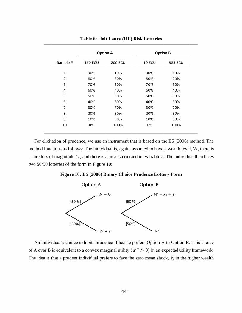
44
Table 6: Holt Laury (HL) Risk Lotteries
For elicitation of prudence, we use an instrument that is based on the ES (2006) method. The
method functions as follows: The individual is, again, assumed to have a wealth level, W, there is
a sure loss of magnitude 𝑘1, and there is a mean zero random variable 𝜀̃. The individual then faces
two 50/50 lotteries of the form in Figure 10:
Figure 10: ES (2006) Binary Choice Prudence Lottery Form
An individual’s choice exhibits prudence if he/she prefers Option A to Option B. This choice
of A over B is equivalent to a convex marginal utility (𝑢′′′ > 0) in an expected utility framework.
The idea is that a prudent individual prefers to face the zero mean shock, 𝜀̃, in the higher wealth
Option A
Option B
Gamble # 160 ECU 200 ECU 10 ECU 385 ECU
1 90% 10%
90% 10%
2 80% 20%
80% 20%
3 70% 30%
70% 30%
4 60% 40%
60% 40%
5 50% 50%
50% 50%
6 40% 60%
40% 60%
7 30% 70%
30% 70%
8 20% 80%
20% 80%
9 10% 90%
10% 90%
10 0% 100%
0% 100%
Option A Option B
𝑊 − 𝑘1
[50 %]
[50%]
𝑊 + 𝜀̃
𝑊 − 𝑘1 + 𝜀̃
[50 %]
[50%]
𝑊
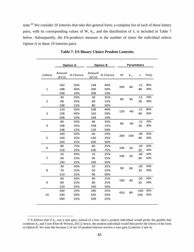
45
state.40 We consider 10 lotteries that take this general form; a complete list of each of these lottery
pairs, with its corresponding values of W, 𝑘1, and the distribution of 𝜀̃, is included in Table 7
below. Subsequently, the ES-prudence measure is the number of times the individual selects
Option A in these 10 lotteries pairs.
Table 7: ES Binary Choice Prudent Lotteries
40 It follows that if 𝑘1 was a sure gain, instead of a loss, then a prudent individual would prefer the gamble that
combines 𝑘1 and 𝜀̃ (see Ebert & Wiesen, 2011); hence, the prudent individual would then prefer the lottery of the form
in Option B. We note this because 2 of our 10 prudent lotteries involve a sure gain (Lotteries 3 and 4).
LotteryAmount
(ECU)% Chance
Amount
(ECU)% Chance W k 1 ε Pr(ε)
160 50% 148 40% -12 80%
1 188 40% 200 50% 48 20%
248 10% 208 10%
40 50% 28 35% -12 70%
2 68 35% 68 15% 28 30%
108 15% 80 50%
120 50% 108 40% -12 80%
3 148 40% 160 50% 48 20%
208 10% 168 10%
80 50% 68 35% -12 70%
4 108 35% 108 15% 28 30%
148 15% 120 50%
100 50% 60 25% -40 50%
5 160 25% 140 25% 40 50%
240 25% 200 50%
80 75% 60 25% -20 50%
120 25% 100 75% 20 50%
50 50% 10 25% -40 50%
7 60 25% 90 25% 40 50%
140 25% 100 50%
30 50% 10 25% -20 50%
8 70 25% 50 25% 20 50%
110 25% 90 50%
60 50% 40 25% -20 50%
9 80 25% 80 25% 20 50%
120 25% 100 50%
260 25% 180 25% -160 50%
10 340 50% 420 50% 160 50%
580 25% 500 25%
Option A Option B
80
6
100 50
100 20
200 100
-40
Parameters
200 40
80 40
120 -40
90 60
100 40
420 80

46
Appendix B – Experimental Instructions for Contextually Framed Condition
EXPERIMENTAL INSTRUCTIONS
BUYER
PART I: THE BARGAINING TASK
You have been randomly assigned the role of Buyer, and you will remain in this role for the
rest of the experiment. You will be randomly and anonymously paired with another participant
who has been assigned the role of Seller. In this task, the seller has been endowed with a plot of
land. As the buyer, you are trying to purchase the land from the seller. You and the seller will be
given an opportunity to bargain over the price of the land (the specific bargaining process is
described below). If you are unable to reach an agreement, then you and the seller will go to court,
where the seller will be forced to sell the land to you. If you go to court, then you, as the buyer,
will receive a fixed payment for acquiring the land. The price the seller receives for the land will
be randomly determined by the court (the specific process of how the court amount is determined
is described in more detail below).
Bargaining with the Seller:
In the experiment, we will be using a fictitious currency called: Thaler. Throughout the
experiment your earnings will be in terms of Thalers, which will then be converted at the end of
the experiment into dollars at a rate of: 10 Thaler to $1. As the buyer, your value for the plot of
land is: 200 Thalers. Your earnings from acquiring the land from the seller will be your value of
200 Thaler minus the price you pay. You and the seller will have an opportunity to bargain over
the price of the plot of land. The bargaining process will work as follows:
Buyer: You will first make an offer (in Thalers) to the seller for the land.
Seller: The seller will then decide whether or not to accept or reject your offer.
If the seller accepts offer then you acquire the land at the price you offered, and your earnings are:
200 - the accepted offer. The seller receives the accepted offer as payment for the land.
If the seller does not accept your offer, then you and the seller will go to court, where the seller
is forced to sell the land to you. You will have to pay a fixed payment of 150 Thaler for the land.
So your earning, if you have to go to court, will be: 200 – 150 = 50. The amount of money that the
seller will receive for the land will depend on how much money the court awards the seller. The
exact amount that the seller will receive will be determined randomly based on the possible court
award amounts and the likelihood that these possible amounts are awarded, which is described
below.
The Court Award:
In the event that an agreement is not reached in the bargaining stage, because the seller rejects
your offer, the court will randomly determine how much the seller will receive. The possible
amounts that the seller may be awarded, and the likelihood that each of these possible amounts is
awarded to the seller will be displayed in a court award table. Below is an example of what one of
these court award tables might look like:
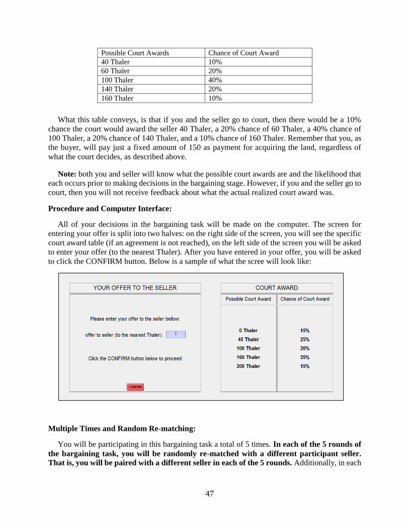
47
Possible Court Awards Chance of Court Award
40 Thaler 10%
60 Thaler 20%
100 Thaler 40%
140 Thaler 20%
160 Thaler 10%
What this table conveys, is that if you and the seller go to court, then there would be a 10%
chance the court would award the seller 40 Thaler, a 20% chance of 60 Thaler, a 40% chance of
100 Thaler, a 20% chance of 140 Thaler, and a 10% chance of 160 Thaler. Remember that you, as
the buyer, will pay just a fixed amount of 150 as payment for acquiring the land, regardless of
what the court decides, as described above.
Note: both you and seller will know what the possible court awards are and the likelihood that
each occurs prior to making decisions in the bargaining stage. However, if you and the seller go to
court, then you will not receive feedback about what the actual realized court award was.
Procedure and Computer Interface:
All of your decisions in the bargaining task will be made on the computer. The screen for
entering your offer is split into two halves: on the right side of the screen, you will see the specific
court award table (if an agreement is not reached), on the left side of the screen you will be asked
to enter your offer (to the nearest Thaler). After you have entered in your offer, you will be asked
to click the CONFIRM button. Below is a sample of what the scree will look like:
Multiple Times and Random Re-matching:
You will be participating in this bargaining task a total of 5 times. In each of the 5 rounds of
the bargaining task, you will be randomly re-matched with a different participant seller.
That is, you will be paired with a different seller in each of the 5 rounds. Additionally, in each

48
of the 5 rounds, the possible court awards and/or the likelihood that each occurs will be different
so be sure to look at the court award table before making your offer.
PART II: THE LOTTERY CHOICE TASK:
After you have finished the 5 rounds of the bargaining task, you will proceed to the lottery task
part of the experiment. In this lottery task, you will make a decision in a series of 30 lottery choices
problems. In each of the 30 lottery choice problems, there will be two possible lottery options,
which will denote as: OPTION A AND OPTION B. Each of these lottery options will involve
possible amounts of Thaler that you could earn and the corresponding likelihood (expressed as a
probability) that you would win that amount. For each of the 30 different lottery problems, you
will be asked to select the option that you most prefer of the two options.
Procedure and Computer Interface:
For each of the 30 lottery choice problems, you will see a screen that displays OPTION A on
the left and OPTION B on the right, with the corresponding possible amounts of Thaler and the %
chance of winning that amount for each option. You will make your preferred choice between the
two options by simply clicking the corresponding button below the option. You will proceed in
this manner through all 30 lottery choice problems, and this will conclude the experiment. Below
is a screen shot of a sample lottery choice problem:
In the above sample lottery problem, if you choose OPTION A, then there is a 50% chance you
would win 160 Thaler, a 40% chance you would win 188 Thaler, and a 10% chance you would
win 248 Thaler. If you choose OPTION B, then there is a 40% chance you would win 148 Thaler,
a 50% chance you would win 200 Thaler, and a 10% chance you would win 208 Thaler.
FINAL PAYMENT:
Your total earnings for this experiment will be determined as follows: First, you will receive $5
for showing up and participating in the experiment. In addition, you will be paid your earnings
(converted from Thalers to dollar at a rate of 10 Thaler to $1) in either one randomly drawn round

49
of the bargaining task or one randomly drawn lottery choice problem from the lottery choice task.
This randomized payment will work as follows: First, after the experiment has ended, an
experimenter will flip a coin to determine whether the bargaining task or the lottery task will be
paid. Thus, each of the tasks is equally likely to be selected for payment. If it is heads then all
participants will get paid for the bargaining task, and if it is tails then the lottery task will be paid.
If the bargaining task is selected, then an experimenter will come to your carrel where you will
individually draw 1 ping pong ball from a bag that contains 5 balls, each one labeled for each of
the 5 rounds. You will then be paid the earnings that correspond to the round that you selected.
If the lottery task is selected, then an experimenter will come to your carrel where you will
individually draw 1 ping pong ball from a bag that contains 30 balls, each one labeled for each of
the 30 lottery choice problems. You will then role two 10 sided dice to determine the amount that
you will win, which will be based on the option that you actually choose for the lottery problem
that you selected. The experimenter will have a sheet that displays which numbers of the die role
correspond to which amount won (these die numbers are selected in a way to generate the same %
chance of winning that is displayed in the option you selected).
After you have finished the experiment, please remain quietly seated until an experimenter
comes to your carrel to determine your earnings. You will then be paid you total earnings in cash.
After you have been paid you may quietly exit the lab.
THANK YOU FOR YOU PARTICIPATION AND COOPERATION
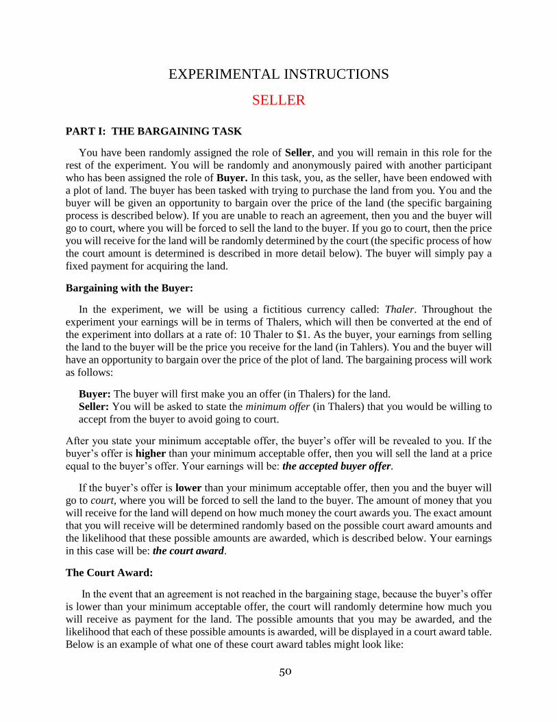
50
EXPERIMENTAL INSTRUCTIONS
SELLER
PART I: THE BARGAINING TASK
You have been randomly assigned the role of Seller, and you will remain in this role for the
rest of the experiment. You will be randomly and anonymously paired with another participant
who has been assigned the role of Buyer. In this task, you, as the seller, have been endowed with
a plot of land. The buyer has been tasked with trying to purchase the land from you. You and the
buyer will be given an opportunity to bargain over the price of the land (the specific bargaining
process is described below). If you are unable to reach an agreement, then you and the buyer will
go to court, where you will be forced to sell the land to the buyer. If you go to court, then the price
you will receive for the land will be randomly determined by the court (the specific process of how
the court amount is determined is described in more detail below). The buyer will simply pay a
fixed payment for acquiring the land.
Bargaining with the Buyer:
In the experiment, we will be using a fictitious currency called: Thaler. Throughout the
experiment your earnings will be in terms of Thalers, which will then be converted at the end of
the experiment into dollars at a rate of: 10 Thaler to $1. As the buyer, your earnings from selling
the land to the buyer will be the price you receive for the land (in Tahlers). You and the buyer will
have an opportunity to bargain over the price of the plot of land. The bargaining process will work
as follows:
Buyer: The buyer will first make you an offer (in Thalers) for the land.
Seller: You will be asked to state the minimum offer (in Thalers) that you would be willing to
accept from the buyer to avoid going to court.
After you state your minimum acceptable offer, the buyer’s offer will be revealed to you. If the
buyer’s offer is higher than your minimum acceptable offer, then you will sell the land at a price
equal to the buyer’s offer. Your earnings will be: the accepted buyer offer.
If the buyer’s offer is lower than your minimum acceptable offer, then you and the buyer will
go to court, where you will be forced to sell the land to the buyer. The amount of money that you
will receive for the land will depend on how much money the court awards you. The exact amount
that you will receive will be determined randomly based on the possible court award amounts and
the likelihood that these possible amounts are awarded, which is described below. Your earnings
in this case will be: the court award.
The Court Award:
In the event that an agreement is not reached in the bargaining stage, because the buyer’s offer
is lower than your minimum acceptable offer, the court will randomly determine how much you
will receive as payment for the land. The possible amounts that you may be awarded, and the
likelihood that each of these possible amounts is awarded, will be displayed in a court award table.
Below is an example of what one of these court award tables might look like:

51
Possible Court Awards Chance of Court Award
40 Thaler 10%
60 Thaler 20%
100 Thaler 40%
140 Thaler 20%
160 Thaler 10%
What this table conveys, is that if you and the buyer go to court, then there would be a 10%
chance the court would award you 40 Thaler, a 20% chance of 60 Thaler, a 40% chance of 100
Thaler, a 20% chance of 140 Thaler, and a 10% chance of 160 Thaler.
Note: both you and buyer will know what the possible court awards are and the likelihood that
each occurs prior to making decisions in the bargaining stage.
Procedure and Computer Interface:
All of your decisions in the bargaining task will be made on the computer. The screen for
entering the minimum offer that you are willing to accept is split into two halves: on the right side
of the screen, you will see the specific court award table (if an agreement is not reached), on the
right side of the screen you will be asked to enter your minimum acceptable offer (to the nearest
Thaler). After you have entered your minimum acceptable offer, you will be asked to click the
CONFIRM button. Below is a sample of what the scree will look like:
Multiple Times and Random Re-matching:
You will be participating in this bargaining task a total of 5 times. In each of the 5 rounds of
the bargaining task, you will be randomly re-matched with a different participant buyer.
That is, you will be paired with a different buyer in each of the 5 rounds. Additionally, in each

52
of the 5 rounds, the possible court awards and/or the likelihood that each occurs will be different
so be sure to look at the court award table before making your offer. If you do go to court in a
particular round, you will not be informed about the actual realized court award until after the
experiment has ended and payments are determined.
PART II: THE LOTTERY CHOICE TASK:
After you have finished the 5 rounds of the bargaining task, you will proceed to the lottery task
part of the experiment. In this lottery task, you will make a decision in a series of 30 lottery choices
problems. In each of the 30 lottery choice problems, there will be two possible lottery options,
which will denote as: OPTION A AND OPTION B. Each of these lottery options will involve
possible amounts of Thaler that you could earn and the corresponding likelihood (expressed as a
probability) that you would win that amount. For each of the 30 different lottery problems, you
will be asked to select the option that you most prefer of the two options.
Procedure and Computer Interface:
For each of the 30 lottery choice problems, you will see a screen that displays OPTION A on
the left and OPTION B on the right, with the corresponding possible amounts of Thaler and the %
chance of winning that amount for each option. You will make your preferred choice between the
two options by simply clicking the corresponding button below the option. You will proceed in
this manner through all 30 lottery choice problems, and this will conclude the experiment. Below
is a screen shot of a sample lottery choice problem:
In the above sample lottery problem, if you choose OPTION A, then there is a 50% chance you
would win 160 Thaler, a 40% chance you would win 188 Thaler, and a 10% chance you would
win 248 Thaler. If you choose OPTION B, then there is a 40% chance you would win 148 Thaler,
a 50% chance you would win 200 Thaler, and a 10% chance you would win 208 Thaler.

53
FINAL PAYMENT:
Your total earnings for this experiment will be determined as follows: First, you will receive $5
for showing up and participating in the experiment. In addition, you will be paid your earnings
(converted from Thalers to dollar at a rate of 10 Thaler to $1) in either one randomly drawn round
of the bargaining task or one randomly drawn lottery choice problem from the lottery choice task.
This randomized payment will work as follows: First, after the experiment has ended, an
experimenter will flip a coin to determine whether the bargaining task or the lottery task will be
paid. Thus, each of the tasks is equally likely to be selected for payment. If it is heads then all
participants will get paid for the bargaining task, and if it is tails then the lottery task will be paid.
If the bargaining task is selected, then an experimenter will come to your carrel where you will
individually draw 1 ping pong ball from a bag that contains 5 balls, each one labeled for each of
the 5 rounds. You will then be paid the earnings that correspond to the round that you selected. If
in the round that you selected you went to court, then you will then role two 10 sided dice to
determine the amount you will be awarded, which will be based on the specific court award table
from that round. The experimenter will have a sheet that displays which numbers of the die role
correspond to which court awards (these die numbers are selected in a way to generate the same
% chance of winning that is displayed in the specific court award table from that round).
If the lottery task is selected, then an experimenter will come to your carrel where you will
individually draw 1 ping pong ball from a bag that contains 30 balls, each one labeled for each of
the 30 lottery choice problems. Again, you will then role two 10 sided die to determine the amount
that you will win, which will be based on the option that you actually choose for the lottery problem
that you selected. The experimenter will have a sheet that displays which numbers of the die role
correspond to which amount won (these die numbers are selected in a way to generate the same %
chance of winning that is displayed in the option you selected).
After you have finished the experiment, please remain quietly seated until an experimenter
comes to your carrel to determine your earnings. You will then be paid you total earnings in cash.
After you have been paid you may quietly exit the lab.
THANK YOU FOR YOU PARTICIPATION AND COOPERATION

54
Appendix C – Experimental Instructions for Abstractly Framed Condition
EXPERIMENTAL INSTRUCTIONS
PLAYER A (BUYER ANALOG)
PART I: THE BARGAINING TASK
You have been randomly assigned the role of Player A, and you will remain in this role for the
rest of the experiment. You will be randomly and anonymously paired with another participant
who has been assigned the role of Player B. In this task, Player B has been endowed with one
fictitious token. As Player A, you are trying to purchase this token from Player B. You and Player
B will be given an opportunity to bargain over the price of the token (the specific bargaining
process is described below). If you are unable to reach an agreement, then you will be given the
token, and you will pay a predetermined fixed amount for acquiring the token. The price the seller
will receive as compensation for the token will be randomly determined by a draw from a lottery
(the process of how the lottery amount is determined is described in detail below).
Bargaining with Player B:
In the experiment, we will be using an experimental currency called: Thaler. Throughout the
experiment your earnings will be in terms of Thalers, which will then be converted at the end of
the experiment into dollars at a rate of: 10 Thaler to $1. As Player A, your value for the token is:
200 Thalers. Your earnings from acquiring the token from Player B will be your value of 200
Thaler minus the price you pay. You and Player B will have an opportunity to bargain over the
price of the token. The bargaining process will work as follows:
Player A: You will first make a price offer (in Thalers) to Player B for the token.
Player B: Player B will then decide whether or not to accept or reject your price offer.
If Player B accepts your offer, then you acquire the token at the price you offered, and your
earnings are: 200 - the accepted price offer. Player B receives the accepted offer as payment for
the token.
If Player B does not accept your offer, then you will be given the token. You will have to pay a
fixed payment of 150 Thaler for the token. So your earning, if you and Player B do not reach an
agreement, will be: 200 – 150 = 50. The amount of money that Player B will receive for the token
will depend on the draw of the lottery that Player B faces as compensation for the token. The exact
amount that Player B will receive will be determined randomly based on the possible outcomes of
the lottery and the likelihood (expressed as a % chance) that these outcomes occur, which is
described below.
The Lottery:
In the event that an agreement is not reached in the bargaining stage, because Player B rejects
your offer, a random draw from a lottery determines how much Player B receives for the token.
The possible amounts that Player B may receive, and the likelihood that Player B receives each of
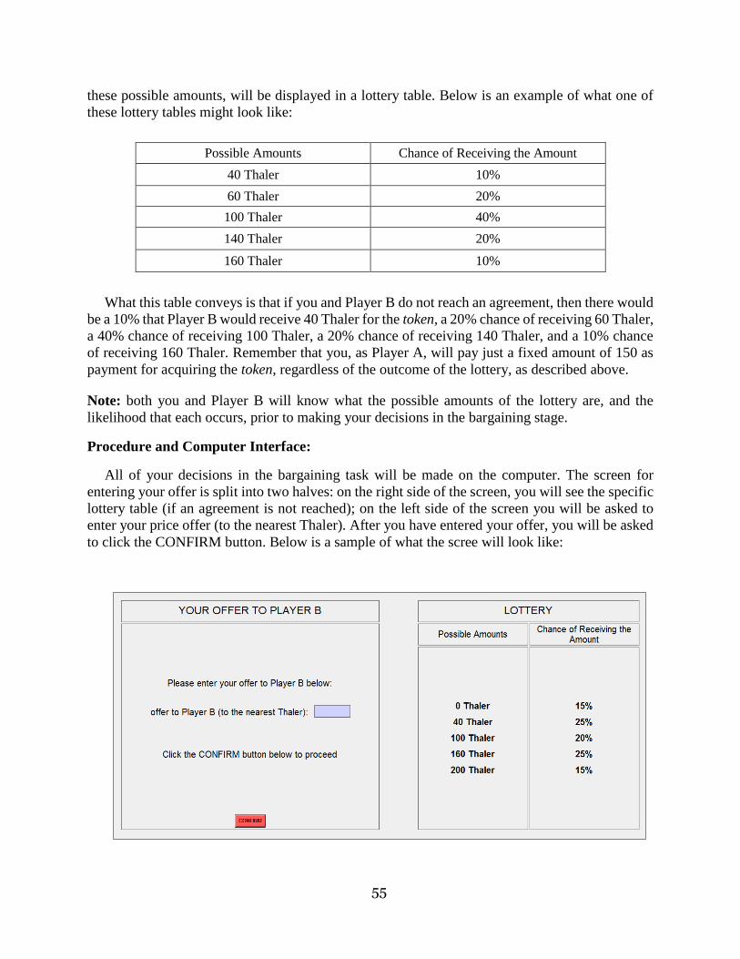
55
these possible amounts, will be displayed in a lottery table. Below is an example of what one of
these lottery tables might look like:
Possible Amounts Chance of Receiving the Amount
40 Thaler 10%
60 Thaler 20%
100 Thaler 40%
140 Thaler 20%
160 Thaler 10%
What this table conveys is that if you and Player B do not reach an agreement, then there would
be a 10% that Player B would receive 40 Thaler for the token, a 20% chance of receiving 60 Thaler,
a 40% chance of receiving 100 Thaler, a 20% chance of receiving 140 Thaler, and a 10% chance
of receiving 160 Thaler. Remember that you, as Player A, will pay just a fixed amount of 150 as
payment for acquiring the token, regardless of the outcome of the lottery, as described above.
Note: both you and Player B will know what the possible amounts of the lottery are, and the
likelihood that each occurs, prior to making your decisions in the bargaining stage.
Procedure and Computer Interface:
All of your decisions in the bargaining task will be made on the computer. The screen for
entering your offer is split into two halves: on the right side of the screen, you will see the specific
lottery table (if an agreement is not reached); on the left side of the screen you will be asked to
enter your price offer (to the nearest Thaler). After you have entered your offer, you will be asked
to click the CONFIRM button. Below is a sample of what the scree will look like:

56
Multiple Rounds and Random Re-matching:
You will be participating in this bargaining task a total of 5 times. In each of the 5 rounds of
the bargaining task, you will be randomly re-matched with a different Player B. That is, you
will be paired with a different Player B in each of the 5 rounds. Additionally, in each of the 5
rounds, the possible lottery amounts and/or the chance of receiving the amount will be different,
so be sure to look at the lottery table before making your offer. In the event that you and Player B
don’t reach an agreement and Player B’s payment is determined by the lottery, you will not receive
feedback about the actual realized outcome of the lottery.
PART II: THE LOTTERY CHOICE TASK:
After you have finished the 5 rounds of the bargaining task, you will proceed to the lottery task
part of the experiment. In this lottery task, you will make a decision in a series of 30 lottery choices
problems. In each of the 30 lottery choice problems, there will be two possible lottery options,
which will be denoted as: OPTION A and OPTION B. Each of these lottery options will involve
possible amounts of Thaler that you could earn and the corresponding likelihood (expressed as a
% chance) that you would win that amount. For each of the 30 different lottery problems, you will
be asked to select which of the two options that you most prefer.
Procedure and Computer Interface:
For each of the 30 lottery choice problems, you will see a screen that displays OPTION A on
the left and OPTION B on the right, with the corresponding possible amounts of Thaler and the %
chance of winning that amount for each option. You will make your preferred choice between the
two options by simply clicking the corresponding button below the option. You will proceed in
this manner through all 30 lottery choice problems, and this will conclude the experiment. Below
is a screen shot of a sample lottery choice problem:
In the above sample lottery problem, if you choose OPTION A, then there is a 50% chance you
would win 160 Thaler, a 40% chance you would win 188 Thaler, and a 10% chance you would
win 248 Thaler. If you choose OPTION B, then there is a 40% chance you would win 148 Thaler,
a 50% chance you would win 200 Thaler, and a 10% chance you would win 208 Thaler.

57
FINAL PAYMENT:
Your total earnings for this experiment will be determined as follows: First, you will receive $5
for showing up and participating in the experiment. In addition, you will be paid your earnings
(converted from Thalers to dollar at a rate of: 10 Thaler to $1) in either one randomly drawn round
of the bargaining task or one randomly drawn lottery choice problem from the lottery choice task.
This randomized payment will work as follows: First, after the experiment has ended, an
experimenter will flip a coin to determine whether the bargaining task or the lottery task will be
paid. Thus, each of the two tasks is equally likely to be selected for payment. If it is heads, then
all participants will get paid for the bargaining task; if it is tails, then all participants will get paid
for the lottery task.
If the bargaining task is selected, then an experimenter will come to your carrel where you will
individually draw 1 ping pong ball from a bag that contains 5 balls, each one labeled for each of
the 5 rounds. You will then be paid the earnings that correspond to the round that you selected.
If the lottery task is selected, then an experimenter will come to your carrel where you will
individually draw 1 ping pong ball from a bag that contains 30 balls, each one labeled for each of
the 30 lottery choice problems. You will then role two 10-sided die to determine the amount that
you will win, which will be based on the option that you actually choose from the lottery problem
that you selected. The experimenter will have a sheet that displays which numbers of the die role
correspond to which amount won (these die numbers are selected in a way to generate the same %
chance of winning that is displayed in the option you selected).
After you have finished the experiment, please remain quietly seated until an experimenter
comes to your carrel to determine your earnings. You will then be paid you total earnings either
by cash or check. After you have been paid you may quietly exit the lab.
THANK YOU FOR YOU PARTICIPATION AND COOPERATION

58
EXPERIMENTAL INSTRUCTIONS
PLAYER B (SELLER ANOLOG)
PART I: THE BARGAINING TASK
You have been randomly assigned the role of Player B, and you will remain in this role for the
rest of the experiment. You will be randomly and anonymously paired with another participant
who has been assigned the role of Player A. In this task, you, as Player B, have been endowed
with one fictitious token. Player A has been tasked with trying to purchase the token from you.
You and Player A will be given an opportunity to bargain over the price of the token (the specific
bargaining process is described below). If you are unable to reach an agreement, then Player A
will be given the token. In return, the price you will receive as compensation for the token will be
randomly determined by a draw from a lottery (the process of how the lottery amount is determined
is described in detail below). Player A will pay a fixed payment for acquiring the token.
Bargaining with Player A:
In the experiment, we will be using a fictitious currency called: Thaler. Throughout the
experiment your earnings will be in terms of Thalers, which will then be converted at the end of
the experiment into dollars at a rate of: 10 Thaler to $1. As Player B, your earnings from selling
the token will be the price you receive for the token (in Thalers). You and Player A will have an
opportunity to bargain over the price of the token. The bargaining process will work as follows:
Player A: Player A will first make you a price offer (in Thalers) for the token.
Player B: You will be asked to state the minimum price offer (in Thalers) that you would be willing
to accept from Player A for the token to avoid having the price be determined by the lottery
After you state your minimum acceptable offer, Player A’s offer will be revealed to you. If
Player A’s offer is higher than your minimum acceptable offer, then you will sell the token at a
price equal to Player A’s offer. Your earnings will be: the accepted offer made by Player A.
If Player A’s offer is lower than your minimum acceptable offer, then Player A will be given
the token. The amount of money that you will receive as compensation for the token will be
randomly determined by a draw from a lottery. The exact amount that you will receive will be
determined randomly based on the possible outcomes of the lottery and the likelihood (expressed
as a % chance) that these outcomes occur, which is described below. Your earnings in this case
will be: the random draw of the lottery.
The Lottery:
In the event that an agreement is not reached in the bargaining stage, because Player A’s offer
is lower than your minimum acceptable offer, the price you will receive for the token will be
randomly determined by a draw from a lottery. The possible amounts that you may receive, and
the likelihood that you receive each of these possible amounts, will be displayed in a lottery table.
Below is an example of what one of these lottery tables might look like:
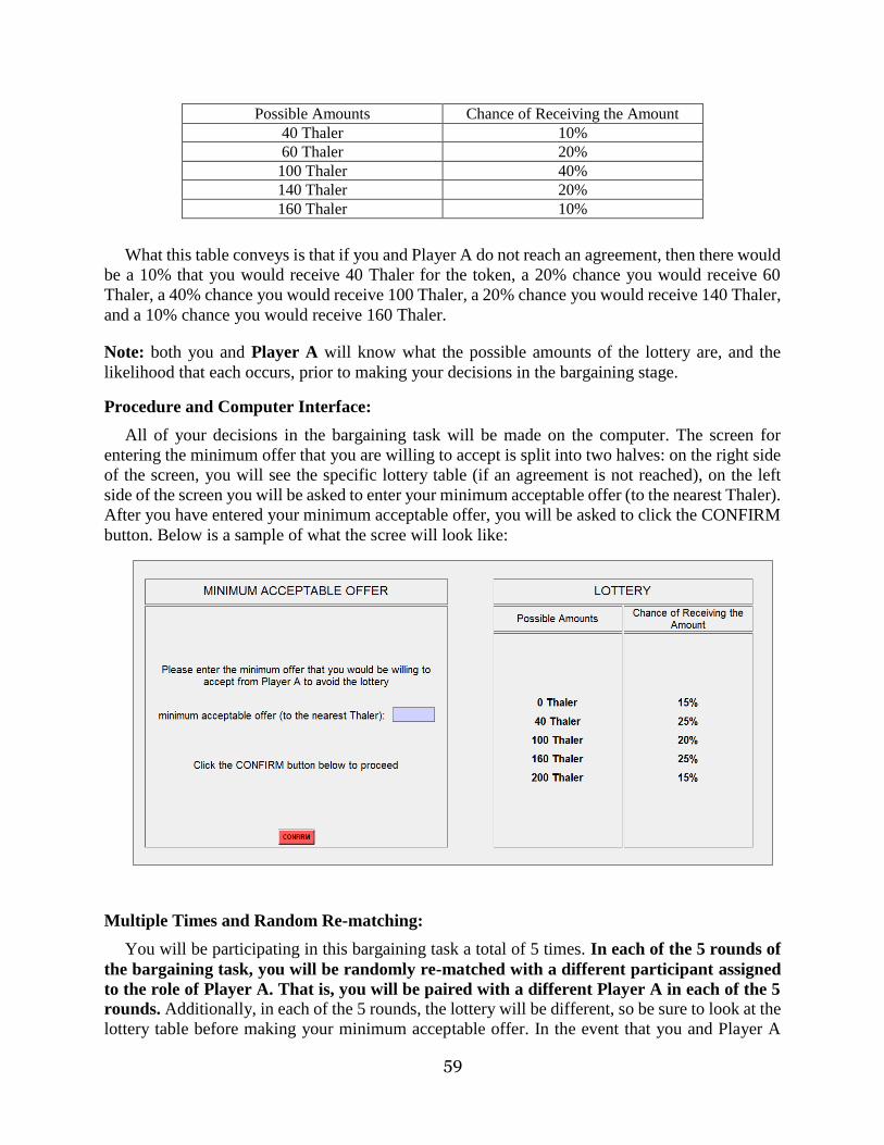
59
Possible Amounts Chance of Receiving the Amount
40 Thaler 10%
60 Thaler 20%
100 Thaler 40%
140 Thaler 20%
160 Thaler 10%
What this table conveys is that if you and Player A do not reach an agreement, then there would
be a 10% that you would receive 40 Thaler for the token, a 20% chance you would receive 60
Thaler, a 40% chance you would receive 100 Thaler, a 20% chance you would receive 140 Thaler,
and a 10% chance you would receive 160 Thaler.
Note: both you and Player A will know what the possible amounts of the lottery are, and the
likelihood that each occurs, prior to making your decisions in the bargaining stage.
Procedure and Computer Interface:
All of your decisions in the bargaining task will be made on the computer. The screen for
entering the minimum offer that you are willing to accept is split into two halves: on the right side
of the screen, you will see the specific lottery table (if an agreement is not reached), on the left
side of the screen you will be asked to enter your minimum acceptable offer (to the nearest Thaler).
After you have entered your minimum acceptable offer, you will be asked to click the CONFIRM
button. Below is a sample of what the scree will look like:
Multiple Times and Random Re-matching:
You will be participating in this bargaining task a total of 5 times. In each of the 5 rounds of
the bargaining task, you will be randomly re-matched with a different participant assigned
to the role of Player A. That is, you will be paired with a different Player A in each of the 5
rounds. Additionally, in each of the 5 rounds, the lottery will be different, so be sure to look at the
lottery table before making your minimum acceptable offer. In the event that you and Player A

60
don’t reach an agreement and your payment is determined by the lottery, you will not be informed
about the actual realized outcome of the lottery draw until after the experiment has ended and
payments are determined.
PART II: THE LOTTERY CHOICE TASK:
After you have finished the 5 rounds of the bargaining task, you will proceed to the lottery task
part of the experiment. In this lottery task, you will make a decision in a series of 30 lottery choices
problems. In each of the 30 lottery choice problems, there will be two possible lottery options,
which will be denoted as: OPTION A and OPTION B. Each of these lottery options will involve
possible amounts of Thaler that you could earn and the corresponding likelihood (expressed as a
probability) that you would win that amount. For each of the 30 different lottery problems, you
will be asked to select the option that you most prefer of the two options.
Procedure and Computer Interface:
For each of the 30 lottery choice problems, you will see a screen that displays OPTION A on
the left and OPTION B on the right, with the corresponding possible amounts of Thaler and the %
chance of winning that amount for each option. You will make your preferred choice between the
two options by simply clicking the corresponding button below the option. You will proceed in
this manner through all 30 lottery choice problems, and this will conclude the experiment. Below
is a screen shot of a sample lottery choice problem:
In the above sample lottery problem, if you choose OPTION A, then there is a 50% chance you
would win 160 Thaler, a 40% chance you would win 188 Thaler, and a 10% chance you would
win 248 Thaler. If you choose OPTION B, then there is a 40% chance you would win 148 Thaler,
a 50% chance you would win 200 Thaler, and a 10% chance you would win 208 Thaler.
FINAL PAYMENT:
Your total earnings for this experiment will be determined as follows: First, you will receive $5
for showing up and participating in the experiment. In addition, you will be paid your earnings
(converted from Thalers to dollar at a rate of 10 Thaler to $1) in either one randomly drawn round
of the bargaining task or one randomly drawn lottery choice problem from the lottery choice task.
This randomized payment will work as follows: First, after the experiment has ended, an
experimenter will flip a coin to determine whether the bargaining task or the lottery task will be

61
paid. Thus, each of the tasks is equally likely to be selected for payment. If it is heads then all
participants will get paid for the bargaining task, and if it is tails then the lottery task will be paid.
If the bargaining task is selected, then an experimenter will come to your carrel where you will
individually draw 1 ping pong ball from a bag that contains 5 balls, each one labeled for each of
the 5 rounds. You will then be paid the earnings that correspond to the round that you selected. If
in the round that you selected an agreement was not reached and your payment is determined by
the lottery, then you will role two 10 sided dice to determine the amount you will receive based on
the corresponding lottery table from that round. The experimenter will have a sheet that displays
which numbers of the die role correspond to which possible outcomes of the lottery (these die
numbers are selected in a way to generate the same % chance of winning that is displayed in the
specific lottery table from that round).
If the lottery task is selected, then an experimenter will come to your carrel where you will
individually draw 1 ping pong ball from a bag that contains 30 balls, each one labeled for each of
the 30 lottery choice problems. Again, you will then role two 10 sided die to determine the amount
that you will win, which will be based on the option that you actually choose for the lottery problem
that you selected. The experimenter will have a sheet that displays which numbers of the die role
correspond to which amount won (these die numbers are selected in a way to generate the same %
chance of winning that is displayed in the option you selected).
After you have finished the experiment, please remain quietly seated until an experimenter
comes to your carrel to determine your earnings. You will then be paid you total earnings either
by cash or check. After you have been paid you may quietly exit the lab.
THANK YOU FOR YOU PARTICIPATION AND COOPERATION