Embed Size (px)
Citation preview
THE IMPACT OF CAPITAL-BASED REGULATION ON BANKTHE IMPACT OF CAPITAL-BASED REGULATION ON BANKRISK-TAKING: A DYNAMIC MODELRISK-TAKING: A DYNAMIC MODEL
Paul S. CalemPaul S. CalemDivision of Research and StatisticsDivision of Research and Statistics
Board of Governors of the Federal Reserve SystemBoard of Governors of the Federal Reserve System
Rafael RobRafael RobDepartment of EconomicsDepartment of Economics
University of PennsylvaniaUniversity of Pennsylvania
March 1996
The views expressed in this paper are those of the authors anddo not necessarily represent the views of the Board of Governors ofthe Federal Reserve System. We thank John Boyd, John Campbell,Mark Carey, David Jones, Myron Kwast, Mark Levonian, John Mingo,Eric Rosengren, and Bruce Smith for helpful suggestions. We thankDavid Jones for supplying us with a copy of his SAS program thatsimulates loan loss distributions. An early version of this paperwas presented at the 1995 ASSA meetings.

AbstractAbstract
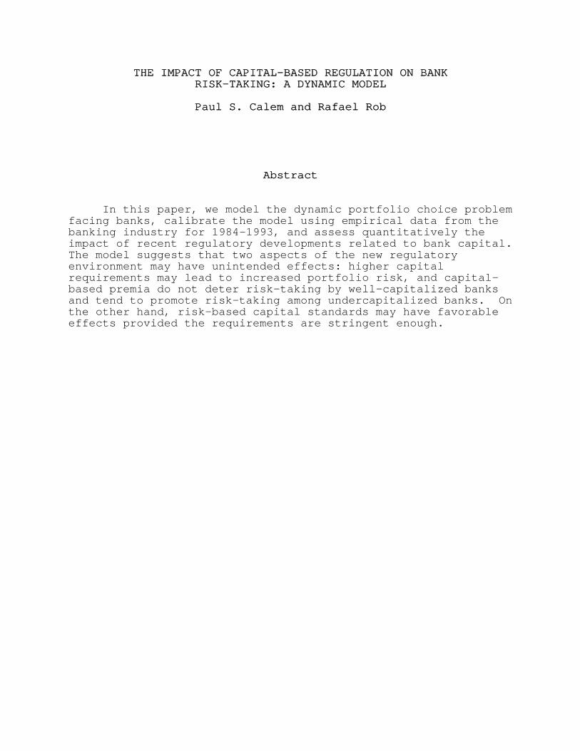
In recent years, new and more stringent federal requlationsgoverning bank capital have been adopted, including insurancepremia linked to banks’ capital-to-asset ratios and capitalrequirements linked to asset portfolio risk. In this paper, wemodel the dynamic portfolio choice problem facing banks, calibratethe model using empirical data from the banking industry for 1984-1993, and assess quantitatively the impact of the new regulations.The model suggests that two aspects of the new regulatoryenvironment may have unintended effects: higher capitalrequirements may lead to increased portfolio risk, and capital-based premia do not deter risk-taking by well-capitalized banks andtend to promote risk-taking among undercapitalized banks. On theother hand, risk-based capital standards may have favorable effectsprovided the requirements are stringent enough.
Bank capital shields the deposit insurance fund from liability by absorbing1
bank losses and preventing bank insolvency. For this reason, capital regulationhas long been a mainstay of banking supervision. Formal capital guidelines,including minimum required ratios of capital to total assets, were instituted bythe federal regulatory agencies in 1981. Prior to that, federal regulators hadsupervised bank capital on a case-by-case basis. See Wall (1989) for furtherdiscussion.
THE IMPACT OF CAPITAL-BASED REGULATION ON BANKTHE IMPACT OF CAPITAL-BASED REGULATION ON BANKRISK-TAKING: A DYNAMIC MODELRISK-TAKING: A DYNAMIC MODEL
1. Introduction1. Introduction
In this article, we consider the impact of increasingly
stringent and complex bank capital regulation on the moral hazard
problem attributed to federal deposit insurance. In recent years,
in the wake of the savings and loan crisis in the U.S., more
stringent and complex capital regulation has been brought to bear
upon federally-insured depository institutions. In 1988, the
federal regulatory agencies adopted "risk-based" capital standards
governing the ratio of capital to "risk-weighted" assets. These
rules replaced simpler requirements pertaining to the ratio of
capital to total assets and, in general, were more stringent than
the old standards, particularly for larger banks (Avery and Berger
1991). In 1991, the Federal Deposit Insurance Corporation1
Improvement Act (FDICIA) was legislated. One important aspect of
the new law was its requirement that the FDIC implement “risk-
related" pricing of deposit insurance. The FDIC responded by
basing insurance premia on capital ratios and supervisory risk
ratings, whereby banks with lower capital ratios and those
assessed by examiners to be more risky pay higher premia. In
addition, the so-called prompt corrective action provisions of
FDICIA established five capital “zones” ranging from “critically

2
To policymakers and regulators, a potential social cost of bank risk-taking2
is the possibility that a major bank failure or series of failures could imposeexternal costs on financial markets. See Bhattacharya and Thakor (1993) andBerger et. al (1994) for further discussion.
undercapitalized” to “well-capitalized,” and required bank
regulators to implement progressively tighter restrictions on bank
activities as capital declines.
These regulatory initiatives were aimed at discouraging bank
risk-taking, preventing bank failures, and ensuring continued
solvency of the deposit insurance fund. In large part, this
expansion of capital-based regulation was an effort to address a
moral hazard problem in banking, widely believed to derive from the
federal deposit guarantee. Moral hazard is seen as arising because
the government guarantee allows banks to make riskier loans without
having to pay higher interest rates on deposits. As a result,
banks may be prone to take on excessive risk. Indeed, there is2
mounting evidence that moral hazard has been a problem under the
current deposit insurance contract; see Berlin, Saunders, and Udell
(1991) and references therein.
In this paper, we attempt a dynamic modeling of the moral
hazard problem and how it might be affected by various regulatory
instruments. The model considers banks which operate in a
multiperiod setting with the objective of maximizing the discounted
value of their profits. In each period, and based on its capital
position, a bank makes a portfolio choice; i.e., it decides how to
allocate its assets between risky and safe investments. Then--as
a result of the bank's portfolio choice, its pre-existing capital

3
One aspect of such a setting is that the bank will want to remain3
solvent and generate future profits, and this will partially offset the moral-hazard problem that the bank is subject to (wanting to exploit a depositinsurance subsidy.) Keeley (1990) presents empirical findings consistent withthe view that the incentive to protect future profits is a moderatinginfluence on bank risk-taking.
position, and the realization of returns on its loans (which is a
random variable)--the bank's capital position for the next period
is determined (and the bank faces again the same portfolio choice
problem, except that its capital position may now be different.)
The goal of the model is to show how banks’ banks portfolio choices
adjust as their capital positions fluctuate over time. Relatedly
(and equivalently), the model shows how portfolio choices differ
among a cross-section of banks distinguished by their current
capital positions. 3
One can reasonably argue that the FDIC’s risk-based premium
assessments are based primarily on ex-post measures of risk, so
that banks undertaking increased risk are assessed higher premia
only in the event that their risk-taking results in losses. To
investigate the incentive effects of the FDIC’s pricing scheme, we
incorporate capital-based premia into our model. The model also
provides a natural framework for analyzing the impact of risk-based
capital regulation, whereby a bank's capital requirement depends on
its portfolio choice. These features are easily embedded into the
model, since the opportunities a bank faces are allowed to depend
on its capital position and on the portfolio choices it makes.
Furthermore, since a bank's capital position varies over time and
since capital positions vary across different banks (within the
same time period), we are able to predict how different banks would
4
Of course, the added capital will mitigate the impact of the increased4
portfolio risk. Nevertheless, the effect of regulatory capital requirements onbank portfolio risk is an important question, because, as emphasized by Bergeret al. (1995), "binding regulatory capital requirements...involve a long-runsocial tradeoff between the benefits of reducing the risk of negative
respond to the imposition of regulatory instruments.
After constructing a theoretical model embodying these
features, we calibrate the model using a set of parameter values
which come from empirical data on the banking sector during the
period 1984-1993. We then numerically solve the model, and apply it
to analyze the impact on bank risk-taking of increased capital
standards, capital-based premia differentials, and risk-based
capital requirements. The model yields a variety of interesting
implications in regard to the efficacy of capital-based regulation.
For instance, we find that a premium surcharge imposed on
undercapitalized banks worsens the moral hazard problem among these
banks, boosting their incentive to take on risk. The underlying
intuition is that the premium surcharge cuts into bank earnings,
hampering the effort to recapitalize. Thus, the premium surcharge
undercuts the ability of an undercapitalized bank to regain a
favorable capital position without undertaking substantial risk.
Surprisingly, however, we find that ex-post pricing of risk as
represented by the premium surcharge has no appreciable impact on
the behavior of a well-capitalized bank.
In the case of a flat (not risk-based) capital requirement, if
the capital requirement is raised, then an ex-ante well capitalized
bank will take on additional portfolio risk as it adds capital in
accordance with the new standard. In most cases, however, an4
5
externalities from bank failures and the costs of reducing bank intermediation."To the extent that capital requirements provide incentives for increased risk-taking, the tradeoff becomes more severe, since "higher capital will be neededto achieve a given level of safety, thus reducing intermediation."
Kahane (1977), Koehn and Santomero (1980), Kim and Santomero (1988),5
Keeton (1988), and Gennotte and Pyle (1991), demonstrate that banks may choosehigher-risk portfolios in response to a higher capital requirement. In themodels of Kareken and Wallace (1978), Furlong and Keeley (1989) and Furlong andKeeley (1990), the deposit insurance subsidy induces a representative bank tohold the riskiest assets available without regard to the minimum capitalstandard.
increase in the capital standard is found to have little impact on
risk-taking behavior among undercapitalized banks. In one
exceptional case, involving a very risky asset having an expected
return lower than the return on the safe asset, we find that an
increased capital standard results in expanded risk-taking among
significantly undercapitalized banks.
We find that an increased risk-based capital standard is
analogous to a higher flat standard, if the risk-based rule is not
too stringent. That is, an ex-ante well capitalized bank will
respond to the increased standard by adding capital and taking on
more portfolio risk. If the risk-based rule is sufficiently
stringent, however, then raising the standard will have a
moderating impact on bank risk-taking. The latter result suggests
that risk-based capital requirements are potentially an effective
way to curtail moral hazard.
Our study differs substantially from previous studies of the
relationship between capital regulation and bank risk-taking.
Previous contributions focused entirely on the impact of a flat
capital standard. Further, the focus of these earlier studies was5
on a representative bank in a static framework with capital set ex-
6
ante at the level required by regulation. Such a framework
precludes consideration of intertemporal consequences of risk-
taking, precludes cross-sectional predictions regarding the
behavior of both well-capitalized and undercapitalized banks, and
cannot be applied to analyze the impact of risk-based capital
regulation.
The paper is organized as follows. The model is constructed
in section 2. Section 3 deals with calibration of the model. In
section 4, we solve the model assuming a flat (not risk-based)
capital standard and flat deposit insurance pricing, and
investigate the impact of varying the calibration holding
regulatory parameters constant. In section 5, we analyze the
effect of a higher minimum capital standard and the impact of
insurance premia penalties. Risk-based capital requirements are
considered in section 6. Section 7 concludes.
2. The Model2. The Model
We consider the dynamics of bank portfolio choice in a multi-
period (infinite horizon) model. Bank size (total assets) is
exogenously set at 1. Assets are funded by deposits D and capital
C; thus, C+D=1. At the beginning of each period, the bank chooses
a portfolio allocation consisting of S units of a safe asset and R
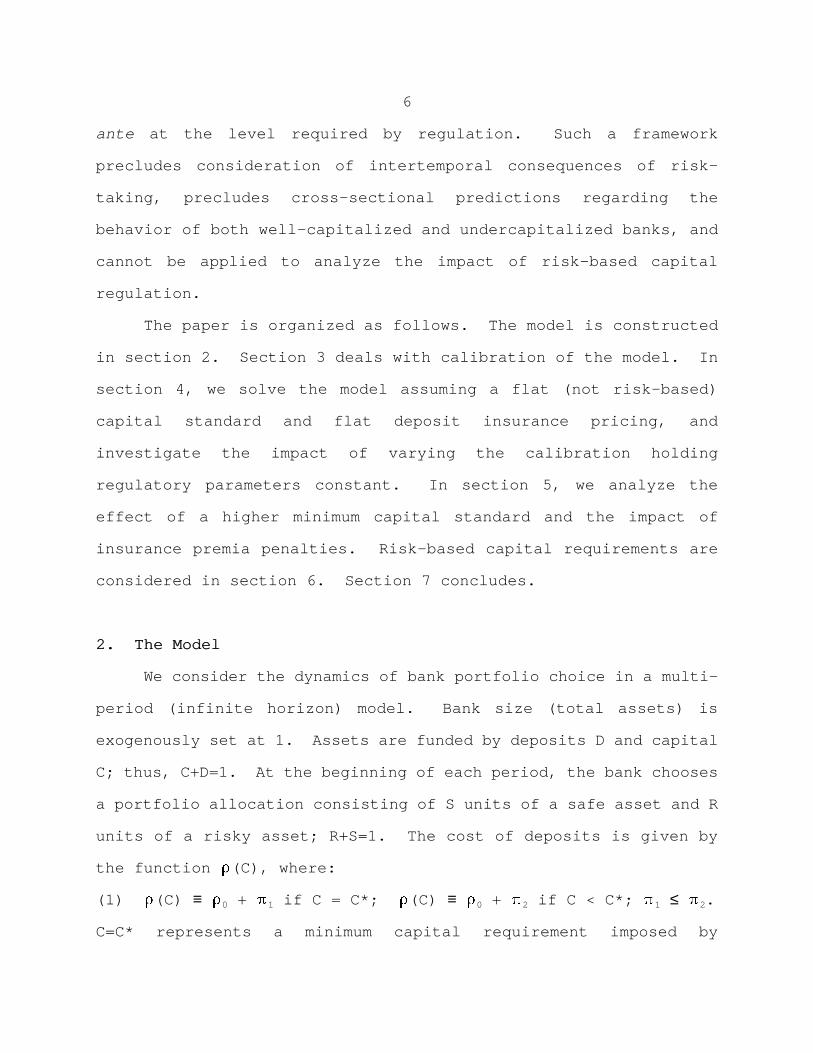
units of a risky asset; R+S=1. The cost of deposits is given by
the function #(C), where:
(1) #(C) ≡ # + ! if C = C*; #(C) ≡ # + ! if C < C*; ! ≤ ! .0 1 0 2 1 2
C=C* represents a minimum capital requirement imposed by

7
regulation. The case ! =! corresponds to fixed rate deposit1 2
insurance premia; the case ! <! corresponds to capital-based1 2
deposit insurance premia (or other "penalties" for falling below
the regulatory capital requirement.) In addition to deposit
expenses, the bank incurs a per-period fixed operating cost F.
The safe asset earns a certain, end-of-period gross return x
> 1 per unit of investment. Ex-ante , the risky asset promises the
gross return y > x per unit invested, but ex-post , a fraction u of0
the investment in the risky asset yields a gross return of 0; i.e.,
this fraction is lost. The remaining fraction, 1 - u, yields the
promised return y . Thus, the realized gross return per unit0
invested in the risky asset is y(u) ≡ y (1 - u). The fractional0
loss u is a random variable taking on values between 0 and 1, drawn
from a distribution with density function g(u) and cumulative
distribution function G(u). Empirical estimates of the various cost
parameters and asset return characteristics (x, F, g, etc.) are
provided in the next section.
In any period, the bank's owners (stockholders) earn the
residual return on the bank's investments after the bank has paid
its depositors, met its fixed expenses, and met the minimum capital
requirement. Formally, let z(C,R,u) denote the return net of
payments to depositors and fixed expenditures that is implied by a
beginning of period capital level C, a portfolio choice R, and a
loss realization u:
(2) z(C,R,u) ≡ x(1 - R) + y(u)R - #(C)(1 - C) - F.
If z(C,R,u) ≥ C*, stockholders earn z(C,R,u) - C*. If 0< z(C,R,u)
8
This assumption is consistent with regulatory requirements mandated by6
FDICIA, whereby undercapitalized banks are prohibited from paying dividends orpaying management fees to a parent holding company.
< C*, the return is insufficient to meet the regulatory capital
requirement, stockholders earn zero, and the entire net return that
period goes toward next period's capital. If z(C,R,u) ≤ 0, the6
bank ceases to exist and the FDIC pays off depositors after
claiming the return on the bank's asset portfolio.
It follows that the set of fractional losses consistent with
continued bank solvency is bounded above by u , where u satisfiesA A
z(C,R,u)=0. Similarly, the set of fractional losses consistent
with positive stockholder earnings is bounded above by u , where B
u satisfies z(C,R,u)=C*. Thus:B
(3) u = [x(1-R) + y R - #(C)(1-C) - F]/y R; A 0 0
(4) u = u - (C*/y R).B A 0
Note that u and u are functions of C and R.A B
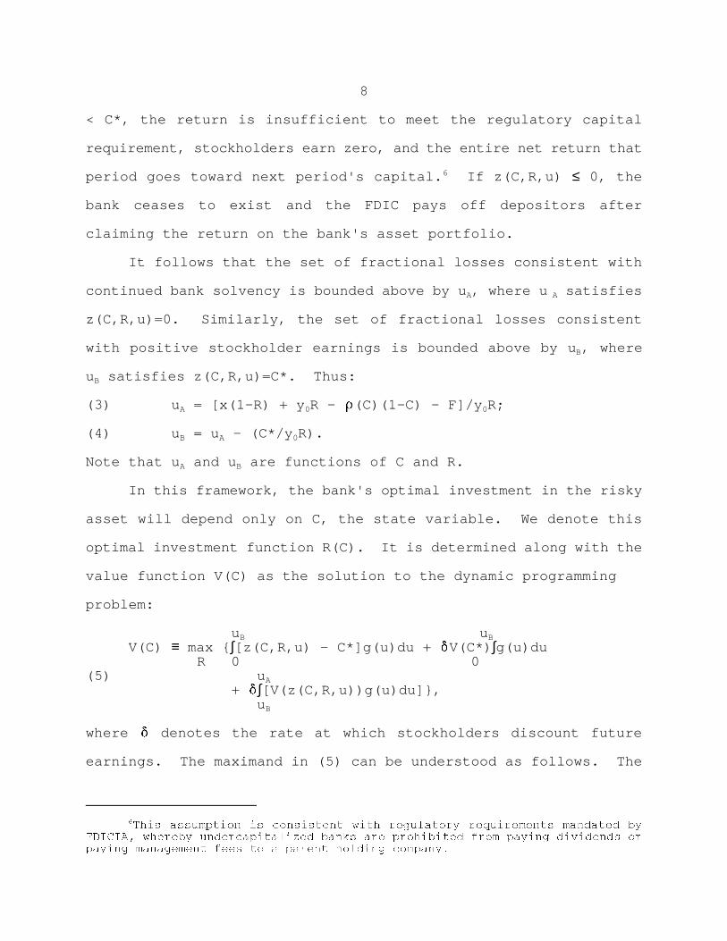
In this framework, the bank's optimal investment in the risky
asset will depend only on C, the state variable. We denote this
optimal investment function R(C). It is determined along with the
value function V(C) as the solution to the dynamic programming
problem:
u uB B
V(C) ≡ max { ∫[z(C,R,u) - C*]g(u)du + V(C*) ∫g(u)du R 0 0
(5) u A
+ ∫[V(z(C,R,u))g(u)du]}, u B
where denotes the rate at which stockholders discount future
earnings. The maximand in (5) can be understood as follows. The

9
first term represents expected current-period earnings, since
stockholders earn z(C,R,u)-C* in the event of a favorable
realization u ≤u and they earn zero otherwise. The second termB
represents the continuation value when the bank meets the capital
requirement at the end of the current period, weighted by the
probability that this will be the case, and the third term is the
expected continuation value when the bank cannot meet the capital
requirement (but is still solvent).
u B
Let E[u u≤u ] = ∫ug(u)du. Since z(C,R,u) - C* = y (u - u), B 0 B
0we can rewrite (5) in the more amenable form:
V(C) = max {u y RG(u ) - Ry E[u u≤u ] + V(C*)G(u )B 0 B 0 B B
R(6) u A
+ ∫[V(z(C,R,u))g(u)du]}. u B
Since (6) is not analytically solvable, we generate a
numerical solution. Towards that, let us discretize the problem as
follows. Define N=C*/0.002 points C along the range of feasiblei
capital positions (0, C*]:
(7) C = 0.002; C = C + 0.002, I=1,...N; N = C*/0.0021 i+1 i
and 20 points R in [0, 1]:j
(8) R = .05; R = R + 0.05, I = 1,...,20.1 i+1 i
In addition, to each C , R , attribute N points u in [u , u ]:i j k B A
(9) u = u - (0.002)k/(1+y )R , k=1,....,N.k A 0 j
Thus, u represents the fractional loss that would leave the bankk
with (0.002)k units of capital at the end of the period, given that
the bank began the period with C units of capital and thei
portfolio position R . Note that C =C*, u =u , and u =u .j N 0 A N B

10
The Fortran programs used to compute the solutions discussed below are7
obtainable from the authors upon request.
The numerical solution to (6) will then be a set of portfolio
positions R*(C ) ≡R and a set of discounted present valuesi i*
V*(C ) ≡V ,I=1,...,N, such that R solves:i i i* *
max { u y R G(u ) - y R E[u u≤u ] + V G(u )B 0 j B 0 j B N B*
R j
(10) N-1+ $ [(V +V )/2)][G(u )-G(u )]}* *
k k+1 k+1 k
k=1
and such that V satisfies (to close approximation):*i
V = u y R G(u ) - y R E[u u≤u ] + V G(u )* * * *i B 0 i B 0 i B N B
(11) N-1 + $ [(V +V )/2][G(u )-G(u )]* *
k k+1 k+1 k
k=1
for each I. Note that u , u , and u in (10) are evaluated at B k k+1
C and R , while u , u , and u in (11) are evaluated at C andi j B k k+1 I
R*(C ). Condition (10) states that for each I, R is the portfolioi I*
allocation that maximizes V(C ), the expected value of current andi
discounted future earnings. The corresponding maximum value of
V(C ) is V as defined by (11). i i*
3. Calibration of the Model3. Calibration of the Model
Computation of a numerical solution to (10) and (11) is
straightforward once a probability distribution G(u) is specified
and parameter values are assigned. Parameters to be calibrated7
include: the deposit interest rate # ; the return x on the safe0
asset; the discount factor ; operating costs F; the ex ante
promised return on the risky asset y ; and the parameters of the0
11
The results are robust to varying these parameters so long as the net8
return on the safe asset (return net of deposit and operating costs) remainssufficiently larger than zero. The solutions converge to maximal risk-taking atall capital levels when the net return on the safe asset approaches zero.
Attention is confined to this period because modifications to the Call9
Reports that were instituted in 1985 introduced certain inconsistencies withearlier years' data. Extreme values were deleted from this panel data set.
Interest expense per dollar of deposits for year [t-1,t] is total deposit10
interest expenses incurred during the period [t-1,t]; i.e., during the year priorto date t, divided by average total deposits for the reporting dates t-1 and t.
specified probability distribution G(u).
Deposit and operating costs and the return on the safe asset .
We assign values to # , x, , and F that are consistent with0
observed data from the banking industry, and hold these constant
for the duration of our analysis. The results are robust to
varying these parameters within a reasonable range. 8
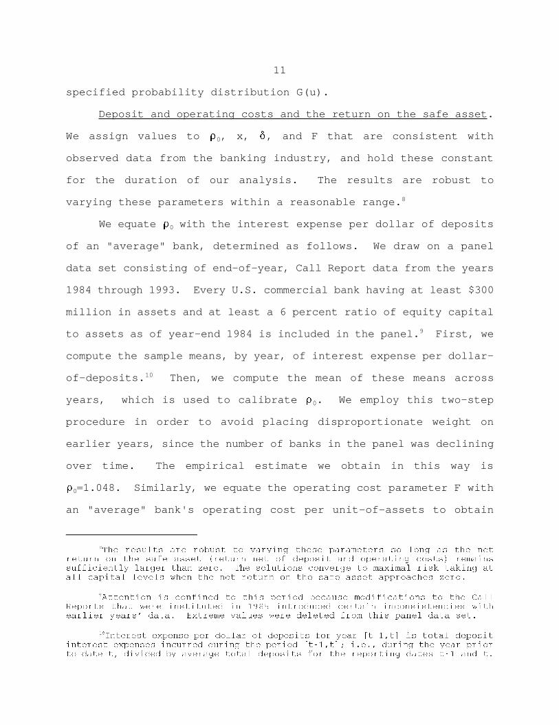
We equate # with the interest expense per dollar of deposits0
of an "average" bank, determined as follows. We draw on a panel
data set consisting of end-of-year, Call Report data from the years
1984 through 1993. Every U.S. commercial bank having at least $300
million in assets and at least a 6 percent ratio of equity capital
to assets as of year-end 1984 is included in the panel. First, we 9
compute the sample means, by year, of interest expense per dollar-
of-deposits. Then, we compute the mean of these means across10
years, which is used to calibrate # . We employ this two-step0
procedure in order to avoid placing disproportionate weight on
earlier years, since the number of banks in the panel was declining
over time. The empirical estimate we obtain in this way is
# =1.048. Similarly, we equate the operating cost parameter F with0
an "average" bank's operating cost per unit-of-assets to obtain
12
We first compute the mean, by year, of annual noninterest expenses net11
of noninterest income divided by total assets (i.e., net noninterest expensesduring [t-1,t] divided by average total assets for dates t-1 and t.) We thencompute the mean of these means across years.
Thus, a low correlation implies that the performances of individual loans12
are nearly independent, in which case the pool default rate will be close to theindividual default probability d. A higher correlation implies that defaults,when they occur, will tend to occur together.
F=0.02. 11
The return on the model's safe asset, net of per-unit
operating costs, is set equal to the average interest rate on 6-
month treasury bills over 1985-1993. Since the 6-month t-bill rate
averaged 1.06 over 1985 through 1993, we set x=1.06+0.020=1.08.
Finally, we set =1/1.06=0.94. Table 1 summarizes these
calibrations.
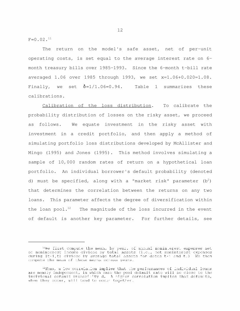
Calibration of the loss distribution . To calibrate the
probability distribution of losses on the risky asset, we proceed
as follows. We equate investment in the risky asset with
investment in a credit portfolio, and then apply a method of
simulating portfolio loss distributions developed by McAllister and
Mingo (1995) and Jones (1995). This method involves simulating a
sample of 10,000 random rates of return on a hypothetical loan
portfolio. An individual borrower's default probability (denoted
d) must be specified, along with a "market risk" parameter (b ) 2
that determines the correlation between the returns on any two
loans. This parameter affects the degree of diversification within
the loan pool. The magnitude of the loss incurred in the event12
of default is another key parameter. For further details, see
13
We adopted the particular approach employed by Jones (1995), whereby a13
loan is invested in a project that yields a random return. A default occurs ifthe return on the project is insufficient to cover the loan repayment; the lossgiven default is assumed to be a fixed proportion of the loan amount. Thecontractual interest rate on a loan has a slight impact on the shape of the lossdistribution generated by this model, since it affects whether a random returnproduces a default.
McAllister and Mingo (1995) and Jones (1995). 13
The loans comprising the model’s risky asset are presumed to
be riskier than the "typical" bank loan. Such a characterization
seems appropriate, as it seems reasonable to draw a distinction
between moral hazard and “normal" bank lending activities. Our
analysis below experiments with alternative parameter
specifications consistent with such a characterization.
Jones (1995) suggests that the average quality of commercial
loans in the portfolios of money center and super-regional banks
lies somewhere in the range corresponding to corporate bonds rated
B through Ba. According to Moody's 1994, loss rates within one
year of issue on B-rated bonds historically have averaged around 8
percent. We adopt this 8 percent figure as a lower bound on the
default probability (d) for the loans comprising our model's risky
asset.
Following McAllister and Mingo (1995), with respect to the
market risk parameter (b ), our analysis focuses on calibrations2
ranging between 20 and 33 percent. These authors indicate that
available data from the banking industry are consistent with
correlations in this range.
The severity of loss given default is assumed to be "business-
cycle dependent". Specifically, the loss distributions utilized
14
The systemic risk factor s is standard normally distributed. The loss14
given default is 30 percent of the dollar amount of exposed principal when s �0. For s < 0, losses are assumed to increase with -s, up to a maximum loss of.80 for s < -2.0.
A bank's default rate for year [t-1,t] is defined to be the ratio of15
problem loans (loans 90 days or more past due and non-accruing loans) to totalloans, calculated at date t. We compute the mean default rate across banks foreach year, and then compute the mean of these means across years, which we taketo be the average loan default rate for the panel. A bank's loss rate for year[t-1,t] is defined to be the ratio of net charge-offs (charge-offs minusrecoveries) during year [t-1,t] divided by average total loans for the reportingdates t-1 and t. We compute the mean loss rate across banks for each year, andthen compute the mean of these means across years, which we take to be theaverage loss rate for the panel.
The standard deviation over time of the annual mean loss rate is16
0.0016, which equals 19 percent of the mean loss rate; the standard deviationover time of the annual mean default rate is 0.0032, equal to 14 percent ofthe mean default rate.
below assume a loss given default of 30 percent given a favorable
outcome of the market risk factor, and a higher loss otherwise, for
an expected loss given default ranging from 40 to 42 percent. 14
This specification of loss given default seems reasonable based on
available data. For instance, drawing on the panel data set
introduced previously, we compute an average loan default rate and
an average net loss rate of 0.0228 and 0.0087, respectively. The 15
latter divided by the former, which might be viewed as a typical
loss given default, equals 0.38. In addition, it is interesting to
note that an independent report by the Society of Actuaries (1993)
finds a 44 percent loss severity (loss per unit of credit exposure)
on defaulted private placement bonds, on average, for issuers rated
BB or lower. Further, the mean across banks of net losses per
dollar loaned exhibits somewhat greater year-to-year variation than
the annual mean default rate. This suggests that the severity of16
losses given default may be affected by the business cycle.
Distributions generated via this approach exhibit a

15
Details regarding the procedure used to calibrate (12) are available from17
the authors upon request.
characteristic shape. Percentiles of one such loss distribution
are shown in column A of table 2. This distribution assumes an 8
percent individual default probability (d), a 33 percent
correlation between loan rates of return (b ), and a loan interest2
rate y =1.14. Column B presents percentiles of the distribution0
obtained when the correlation parameter is reduced to 25 percent.
These distributions rise very slowly through the median and then
become progressively steeper, rising sharply through the upper
percentiles.
Piecewise linear approximation to the distribution . For the
purpose of obtaining numerical solutions to our model, we
approximate each generated loan loss distribution by means of a
piecewise linear distribution with support [u , u ], where u =0:0 8 0
(12) F(u)=(u-u )/(u -u ) if u ≤u≤u ;0 1 0 0 1
F(u)=F(u )+ (u-u )/(u -u ) if u ≤u≤u ; I = 0,...,8.i i i+1 i i i+1
In (12), u ,u ,....u denote, respectively, the 0th, 1st, 5th, 25th,0 1 8
50th, 75th, 95th, 99th, and 100th percentile of the distribution.
To implement each generated loan loss distribution, we approximate
it via appropriate calibration of the parameters u , u in (12). 1 817
Calibration of the promised return on the risky asset . It
remains to calibrate y , the contractual interest rate on loans0
comprising the risky asset. Given a specification of the loan loss
distribution, it might seem reasonable to calibrate y by observing 0
market spreads on loans of comparable riskiness. Data relating
16
Normally, one would expect a risky asset to provide a higher expected18
return than a safe asset. In cases corresponding to more extreme moral hazard,however, the risky asset might have an expected return below the return on thesafe asset. An example of this is considered below.
Among B-rated private-placement bonds (which tend to exhibit narrower19
spreads than B-rated publicly-traded bonds), spreads of 800 basis points or moreover comparable maturity t-bonds are uncommon, although not so uncommon as to beconsidered outliers (Carey and Luckner 1995). Due to the more intensiveinformation production and higher monitoring costs associated with bank loans,however (Carey et. al 1995), one cannot assume that spreads on risky bank loanswould be confined to a similar range.
bank loan spreads to measures of risk are unavailable, however.
Instead, we experiment with various calibrations of y in 0
association with each specified loan loss distribution.
Mostly, we assume that the expected return on the risky asset
would exceed the return on the safe asset by a reasonable amount. 18
Consequently, the calibrations we utilize below generally involve
spreads of 800 basis points or more between y and the average 6-0
month t-bill rate (1.06). Spreads of this size are well within the
realm of plausibility. For instance, U.S. Small Business
Administration (1993) reports that spreads of 800 to 1200 basis
points are not uncommon for short-term, fixed-rate small business
loans. 19
4. Solution under Alternative Calibrations of the Risky Asset4. Solution under Alternative Calibrations of the Risky Asset
In this section, we demonstrate that the solution to the model
tends to be roughly U-shaped, with notable persistence across
alternative calibrations of the probability distribution of returns
on the risky asset. Throughout this section, we assume a flat
deposit insurance premium ( ! =! ) held constant at ! =0.0025, and1 2 1
we hold the minimum capital requirement constant at C*=0.06.
17
Table 3a presents the solution to the model under three
alternative calibrations of the distribution of returns on the
risky asset. Each of these assume an individual default
probability d=0.08 and an ex-ante promised return y =1.145. The0
three specifications differ with respect to the assumed correlation
b between asset returns, which ranges from 0.25 to 0.33.2
Table 3b presents the solution to the model under some
additional calibrations of the distribution of returns on the risky
asset. For these calibrations, the assumed individual default
probability is not held constant but ranges from 0.09 to 0.12, and
the promised return y is assumed to increase with the default0
risk.
The parameters underlying the distribution of returns (d, b , 2
and y ) are listed at the top of each column, and the solution to0
the model under that calibration is indicated below. Also noted at
the top of the column is the corresponding expected return (denoted
Rt) on the risky asset.
The solutions depicted in tables 3a and 3b are roughly U-
shaped, with the amount of risk depending on the bank’s current
capital position. In general, a severely undercapitalized bank
takes maximal risk in an effort to improve its capital position.
This implication of the model provides a formal rationale for the
prompt corrective action provisions of FDICIA, which require
progressively more strict regulatory intervention as a bank’s
18
Banks in capital zone 1 (well capitalized) face no mandatory restrictions20
on activities. Those in zone 2 (adequately capitalized) are subject toincreased regulatory scrutiny, including more frequent supervisory exams andprior FDIC approval to accept brokered deposits. Banks in capital zone 3(undercapitalized) face several mandatory restrictions; for instance, these banksare prohibited from accepting brokered deposits and from paying dividends ormanagement fees, and they are subject to restrictions on asset growth. Those inzone 4 (significantly undercapitalized) are subject to the same restrictions asthose in zone 3 plus several additional ones, including restrictions on inter-affiliate transactions, on deposit interest rates, and on officer compensation.Banks in capital zone 5 (critically undercapitalized) are subject to still morerestrictions, and generally must be placed in receivership or conservatorshipwithin 90 days after being classified as critically undercapitalized.
capital declines. A more modestly undercapitalized bank takes20
much less risk, trying to ensure it doesn't go under. Finally, as
capital rises and the bank is more remote from bankruptcy, the bank
takes on more risk, if the risky asset is associated with a higher
expected return than the safe asset. This characteristic shape can
be understood as follows.
In the case a severely undercapitalized bank, maximal risk-
taking arises because the proportion invested in the risky asset,
whether large or small, does not significantly affect the
probability of insolvency, since only a small erosion of the bank's
capital suffices for insolvency. Rather, incremental risk
primarily affects the loss incurred (by the deposit insurance fund)
in the event of insolvency. On the other hand, unless it
undertakes substantial risk, a severely under-capitalized bank
stands little chance of regaining a favorable capital position.
A less severely undercapitalized bank takes on comparatively
little risk; its predominant concern is to avoid insolvency or
further erosions of capital. For this bank, incremental risk-
taking has a more significant impact on the probability of
(eventual) insolvency, and this bank stands a better chance of
19
regaining a favorable capital position without undertaking-
substantial risk.
A well-capitalized bank can afford to take more risk because
it is more remote from bankruptcy. This bank would stand a good
chance of recovery should it incur an erosion of capital due to
loan losses.
The effects of parameter changes . The solutions are not
highly sensitive to changes in the promised return on the risky
asset (y ), holding other parameters constant. Consider, for0
example, the solution depicted in table 3a, column (I). Small
increases (or decreases) in y above (below) 1.145 yield a modest0
expansion (contraction) of the range of maximal risk-taking among
undercapitalized banks. Within a 50 basis point range (1.1425 ≤ y 0
≤ 1.1475), changes in y have no impact on R*(C*); i.e., on the0
solution as it pertains to a well-capitalized bank. The other
solutions depicted in tables 3a and 3b are no less robust; for
instance, within a 60 basis point range (1.051 ≤ y ≤ 1.057),0
changes in y have little impact on the solution depicted in table0
3b, column (I).
Ultimately, as y declines, the solution collapses to minimal0
risk-taking at all capital levels. Likewise, a sufficiently large
increase in y yields maximal risk-taking at all capital levels.0
Calibrations of y that yield minimal (or maximal) risk-taking at0
all capital levels are of limited interest. Differing regulatory
policies or parameters generally have no impact on the solutions in
these cases. Moreover, minimal (maximal) risk-taking by all banks
20
would seem inconsistent with an equilibrium in the asset market
(although that is outside the scope of our model). With all banks
seeking to invest solely in the safe (risky) asset, one would
expect the contractual interest rate y to be driven up (down) by0
competitive pressures.
A reduction in the correlation of rates of return on risky
loans (b ) yields a contraction of the range of maximal risk-taking2
among undercapitalized banks. This is clearly illustrated by the
solutions depicted in table 3a. With y =1.145, d=0.08, and b =0.33,02
maximal risk-taking arises at all capital levels less than or equal
to 0.008. Holding y and d constant, the range of maximal risk-0
taking contracts as b is reduced to 0.30, and it disappears2
entirely with b =0.25. Moreover, a decrease in the correlation2
parameter b is associated with increased risk-taking by well-2
capitalized banks.
These effects of changing the correlation parameter b can be 2
understood as follows. With an increase in b , the largest 2
potential losses occur with increased probability, but the
likelihood that losses will be only small or negligible also
increases, and the median loss declines. That is, the loss
distribution function becomes more concave; compare, for example,
column A with column B in table 2. The first factor (increased
probability with respect to the largest potential losses) tends to
deter risk-taking by well-capitalized banks. The second factor
tends to encourage risk-taking by undercapitalized banks.
The range of maximal risk-taking also widens with concomitant
21
increases in d and y . Consider, for instance, column (ii) of0
table 3b in comparison to column (iii) of table 3a. The following
intuition underlies this effect. The increase in the ex-ante
interest rate provides an incentive to take on more risk, while the
increased probability of default provides an opposing incentive.
For a bank that is significantly undercapitalized, the former
dominates, because the expected losses associated with the
increased probability of default are borne primarily by the deposit
insurer rather than by the bank.
Comparing column (I) of table 3b to column (ii) of table 3a,
we see again that increases in y and d lead to an expansion of0
risk-taking among undercapitalized banks. Note, in this case, that
the increases in y (from 1.145 to 1.155) and d (from 0.08 to 0.09)0
are assumed to be accompanied by a reduction in b (from 0.30 to2
0.28). Without this assumption, the increases in y and d would 0
make risk-taking so attractive as to yield maximal risk-taking at
all capital levels. Further increases in y (to 1.168) and d (to0
0.11), when accompanied by a further reduction in b (to 0.20), 2
yields the solution depicted in column (iii) of table 3b.
When the expected return on the risky asset is below the risk-
free return, well capitalized banks take on minimum risk; i.e.,
R*(C*)=0.05. Maximal risk-taking may persist, however, among
severely under-capitalized banks. Consider, for instance, the case
depicted in column (iv) of table 3b. In this case, the probability
of default on an individual loan in the risky asset portfolio is
0.15, and the correlation of loan rates of return is 0.33, implying
22
very high risk. Moreover, the expected return on the risky asset
(given the specified y ) is lower than that provided by the safe0
asset. The range of maximal risk-taking among undercapitalized
banks is quite extensive, but at capital levels above this range,
minimal risk-taking is the outcome.
5. Increased Capital Standards and Capital-Based Premia5. Increased Capital Standards and Capital-Based Premia
To analyze the impact of an increase in the capital
requirement, we now solve the model with C*=0.07 in place of
C*=0.06. Table 4 depicts the solutions thus obtained, for several
of the calibrations introduced in the previous section.
Comparing the solutions in table 4 to their counterparts in
tables 3a and 3b, it is clear that when the capital requirement is
raised and an ex-ante well capitalized bank increases its capital
to meet the new standard, the bank generally takes on more
portfolio risk. This is consistent with the overall U-shape of the
solution, whereby beyond the lowest capital levels, risk-taking
tends to increase with capitalization.
Note, however, that the increased regulatory standard appears
to have a moderating effect on risk-taking at some intermediate
capital levels. For example, comparing column (ii) of table 4 to
column (iii) of table 3b, we observe an ex-post decline in risk-
taking (from R*=.50 to R*=.10) at capital levels 0.056<C ≤0.060.
In general, an increase in the capital standard appears to
have little impact on the range of maximal risk-taking among
severely undercapitalized banks. An important exception, however,
23
is the case of extreme moral hazard depicted in table 3b, column
(iv). Recall that in this case, significantly undercapitalized
banks exploit an opportunity to invest in an extremely risky asset
(d=0.15), gambling on a high return. Comparing column (iii) of
table 4 to column (iv) of table 3b, we find that raising the
regulatory capital standard has a deleterious impact in this case;
i.e., the range of maximal risk-taking among undercapitalized banks
expands substantially. Ex-post , banks engage in maximal risk
taking at all capital levels below 4.4 percent. This suggests that
an increase in the minimum capital standard may generate a need for
increased vigilance with respect to supervision of undercapitalized
banks.
Capital-based premia . As noted in the introduction, one
important aspect of FDICIA was its requirement that the FDIC
implement “risk-related" pricing of deposit insurance. The FDIC
responded by basing insurance premia on bank capital ratios and on
supervisory risk ratings that reflect examiner evaluations of bank
earnings, asset quality, liquidity, and management. Banks with
lower capital ratios and those assessed by examiners to be more
risky pay higher premia. These risk-based premia, when first
introduced, ranged from 23 to 31 basis points across risk
categories. Recently, the FDIC amended its deposit insurance
premium regulations to establish a new rate schedule. The new
risk-based premia range from 4 to 31 basis points.
One can reasonably argue that premium assessments under this
regulation are based primarily on ex-post indicators, whereby banks
24
Alternative calibrations of the premium differential yield qualitatively21
simlar results.
undertaking increased risk are assessed higher premia only in the
event that their risk-taking results in losses. To investigate the
incentive effects of such ex-post pricing of risk, we solve the
model assuming a capital-based premium differential, with ! =1
0.0025 and ! = 0.0035, holding C* constant at 0.06. Table 5 221
depicts the solutions thus obtained, for several of the
calibrations examined previously.
Comparison of table 5 with tables 3a and 3b reveals that
introduction of the deposit premium differential has a substantial
impact in the case of significantly undercapitalized banks, in the
direction of increased risk-taking. For example, comparing column
(I) of table 5 to column (I) of table 3a, we observe that the
introduction of the premium differential causes banks at capital
levels greater than 0.008 and less than or equal to 0.030 to jump
from minimal risk-taking (R*=0.05) to holding only risky assets
(R*=1.0). The underlying intuition is that the premium surcharge
cuts into bank earnings, hampering the effort to recapitalize.
Thus, the premium surcharge undercuts the ability of an
undercapitalized bank to regain a favorable capital position
without undertaking substantial risk.
This comparison also indicates that introduction of the
premium differential has, at best, a slight impact on moderately
undercapitalized banks, in the direction of reduced risk-taking.
We observe no impact at all on the behavior a well-capitalized
25
bank; i.e., increasing the premium differential does not appear to
have any deterrent effect on risk-taking among well-capitalized
banks. This result can be understood as follows. Risk-taking in
the model is represented by increased investment in a risky asset.
This asset is characterized by a loss distribution that is highly
skewed and has a long tail (it is leptokurtic ), so that losses only
rarely occur but tend to be very large when they do occur. On the
margin, increased investment in such a risky asset has only a
slight impact on a bank’s probability of becoming undercapitalized.
Consider, for example, the solution depicted in column (I) of table
3a. In this case, a well-capitalized bank invests R*(C*) = 0.55 in
the risky asset and with probability F(u )= 0.78792, remains well-B
capitalized into the subsequent period. If the bank were to reduce
its investment in the risky asset to 0.50, its probability of
remaining well-capitalized would rise to 0.79157, an increase of
only 0.00365.
Hence, in our model the premium penalty associated with
becoming undercapitalized has no appreciable incentive effect on
the behavior of well capitalized banks. An open question, which we
leave to future research to investigate, is whether a similar
result would be obtained if risk-taking were represented as the
inclusion of progressively risky types of assets in a portfolio,
rather than as incremental units of a given asset.
These results are robust to varying any of the calibrations
26
These would be ranges within which the solution under a flat capital22
requirement retains something of a "U-shape" (i.e., does not collapse to minimalrisk-taking at all capital levels or to maximal risk-taking at all capitallevels.)
Primary capital was defined to include equity, loan loss reserves,23
preferred stock, and various kinds of debentures; see Wall (1989) for details.
within reasonable ranges. The results are also robust to assuming22
a higher minimum capital standard, or to modifying the size of the
assumed premium differential. In sum, the primary effect of an
insurance premium surcharge on undercapitalized banks is to
substantially aggravate the moral hazard problem among
undercapitalized banks, and this implication of the model is highly
robust across alternative calibrations.
6. The Impact of Risk-Based Capital Requirements6. The Impact of Risk-Based Capital Requirements
As noted in the introduction, in 1988 the federal regulatory
agencies adopted "risk-based" capital standards that were
effectively more stringent than the prior standards, particularly
for larger banks (Avery and Berger 1991). Under the prior
standards, primary capital had to be at least 6 percent of total
balance sheet assets or the bank would face supervisory action. 23
Under the risk-based standards, differing weights are assigned to
various categories of bank assets (e.g. home mortgage loans,
treasury bills, commercial loans) prior to summing the assets, to
reflect differences in credit risk. The regulations adopted in
1988 required that total capital be at least 8 percent of risk-
weighted assets (where loan loss reserves were no longer to be
fully included as a component of measured capital). In addition,
27
In addition, the 1988 requlation required banks to hold some capital24
against off-balance sheet activities. Banks were directed to comply with the newstandards by 1992. See Wall (1989) for details.
As noted previously (see footnote 20), FDICIA introduced a distinction25
between well capitalized and adequately capitalized (as well as three distinctcategories of undercapitalized), whereby the latter are subject to closerregulatory scrutiny. Thus, for instance, under current regulations, totalcapital has to be at least 8 percent of risk-weighted assets for a bank to beconsidered adquately capitalized, and at least 10 percent of risk-weighted assetsfor a bank to be considered well capitalized. In addition, there are tests forwell capitalized vs. adquately capitalized that are based on tier-one capital inrelation to risk-weighted assets and tier-one capital in relation to totalassets, resepctively.
A bank meeting the three capital ratio tests for the well capitalizedcategory might still be subject to a capital directive requiring it to raiseadditional capital, based on supervisory assessments of its earnings, assetquality, liquidity, and managerial factors. Any such bank would be classifiedas adequately capitalized within the prompt corrective action framework.
these regulations set standards for tier-one capital (a more
restrictive definition of capital) in relation to risk-weighted
assets and for tier-one capital in relation to total assets. 24,25
In this section, we examine the consequences for bank
portfolio choice of risk-weighting of assets in computation of
regulatory capital. Before we proceed, however, a word of caution
is in order. While our model may provide some insight into the
effects of a risk-based capital standard, the model is subject to
an important limitation. In practice, very broad risk-categories
of assets are defined for the purpose of calculating regulatory
capital requirements. For instance, the highest-risk category
would incorporate all of a bank’s commercial and industrial (C and
I) lending. Thus, in practice, a bank might respond to a binding
risk-based requirement primarily by reducing its investment in
assets that, unlike the model's risky asset, may not be excessively
risky. For instance, a bank might curtail moderately risky C and
I lending. Consideration of this issue would require a model with
28
at least three assets (safe, moderately risky, and excessively
risky, respectively), and is therefore outside the scope of the
present paper.
We assume that the risk-based standard takes the simple form
C* = 0.06 + n(R - R ), where R and n are parameters determining0 0
the stringency of the requirement. That is, C* is a linear
function of R, the bank's proportionate investment in the risky
asset. So long as R is no greater than R , required capital equals0
0.06. For R > R , required capital exceeds 0.06 by an amount0
proportional to the gap between R and R . To provide a benchmark0
for evaluating the impact of risk-basing of the capital standard,
we assume that ex-ante , a flat standard C* = 0.06 is in effect, and
that the risk-based standard that is introduced is binding on ex-
ante well capitalized banks.
Further, we assume that the risk-based standard does not apply
to banks that have become significantly undercapitalized. Rather,
regulators would require of such banks a long-run capital target or
capital restoration plan that is independent of their current
portfolio composition. Formally, at capital levels below some
suitably selected threshold level C , the bank becomes subject to0
the flat capital requirement C*=0.06. This assumption simplifies
the analysis because it frees us from having to consider how an
endogenous, risk-based capital standard would affect a severely
undercapitalized bank's incentive to take on maximal risk. It is
also consistent with empirical evidence--in the case of
significantly undercapitalized banks, examiners have tended to
29
Note that R is the proportional investment in the risky asset equating26 k
required capital (under the risk-based standard) with the bank's capital target.
focus on capital in relation to total assets (the leverage ratio)
rather than risk-weighted assets (Peek and Rosengren 1995b, c).
In sum, banks are subject to a capital rule that depends on
their current capital level C and (when C ≥ C ) on the amount of0
risk the bank undertakes:
(13) C* = 0.06 + n(R - R ) if C ≥ C , C* = 0.06 otherwise.0 0
To model the impact of such a capital rule on bank risk, we
substitute (13) for C* in the dynamic optimization problem (6),
which is then solved as follows.
Solution procedure . As a first step, we solve a related
dynamic optimization problem. Let k be a given, non-negative
integer and define:
(14) C = 0.06 + (0.002)k; R = R + (C - 0.06)/n.k k k0
We consider the dynamic optimization problem (6) subject to the
constraints:
(15) C* = C ; R(C) ≤ R if C ≤ C ≤ C .k k k0
An intuitive interpretation of these constraints is that the bank
commits to a self-imposed "capital target" (C ) which governsk
payment of dividends in the same way that a flat, regulatory
standard would. This capital target together with a capital rule
of the form (13) implies an upper bound (R ) on bank risk-taking.k 26
For any given k, computing a numerical solution to this problem is
straightforward. Let R*(C, k) denote this solution.
The next step is to solve (6) subject to (15) for all k within
30
In addition, assume that C > 0.01.27
0
Return-on-equity equals 100(1 - )V(C)/C.28
a relevant range. The solutions R*(C, k) can be examined and
compared to identify R*(C, k*), the solution to the model under the
risk-based capital rule (13). Precisely how this is accomplished
is best understood by means of an example, to which we now turn our
attention.
Numerical computations . Suppose (in regard to the risky
asset) that y = 1.145, d = 0.08, and b = 0.33. In addition, let02
! = ! = 0.0025, and let n=1 and R = 0.50 in (13). First, we1 2 027
derive the solution to (6) under alternative capital targets C as k
defined by (15).
A bank can choose 0.06 as its capital target (k=0), in which
case it faces the constraint R ≤ 0.50 (at capital levels C and 0
above), or it can set a target capital level of 0.062 (k=1),
enabling it to invest up to 0.55 in the risky asset.
Alternatively, the bank can set a target capital level of 0.064
(k=2) and invest up to 0.60 in the risky asset (or it can choose
yet a higher capital target.) The solutions implied by each of
these three alternatives are presented in table 6. Alongside each
solution we provide the associated return-on-equity (ROE) at each
level of capital. 28
Next, we establish that the configuration corresponding to the
capital target of 0.064 (k*=2) represents the actual solution to
the model under the specified capital rule (13). In particular, we
show that regardless of its ex-ante level of capitalization, the
31
bank's equity holders are best off under a commitment to raise bank
capital to 0.064 and to maintain 0.064 as a permanent capital
target, compared to the other two alternatives depicted in table 6.
Consider a bank that, ex-ante , is well capitalized (at capital
level 0.06) and is investing 0.55 in the risky asset (in accordance
with the solution in column I of table 3a). If ex-post the bank
chooses to reduces its investment in the risky asset to 0.50 and
maintain its current level of capitalization, then it will earn an
average ROE of 22.481 (a decline of 0.630 relative to its ex-ante
ROE of 23.111). If the bank opts to build capital to 0.062, then
it will earn a marginal ROE of (23.104+22.563)/2 = 22.8335 on its
unit of reinvested earnings; since this marginal ROE exceeds
22.481, this strategy dominates the first one. However, if the
bank opts to build its capital to 0.064, then it will earn an even
higher marginal ROE: [(23.629+23.091)/2 + (23.091+22.629)/2]/2 =
23.110. Hence, the latter strategy dominates the other two.
Continuing in this manner it is shown that the latter alternative
(0.064) is preferred to any that involves a still higher capital
target. Thus, commitment to a capital target of 0.064 is the
preferred alternative for an ex-ante well capitalized bank, and it
must be likewise for an ex-ante undercapitalized bank, since the
goal of such a bank is to be well-capitalized. Hence, following
the imposition of the capital rule (13), an ex-ante well
capitalized bank commits to increase its capital to 0.064, which
also becomes the capital target for any bank (regardless of initial
capitalization), so that the solution to the model coincides with
32
that under C**=0.064 in table 6. Note that imposition of the
capital rule (13) thus entails increased risk-taking and a higher
effective capital standard, compared to the ex-ante , flat capital
requirement C*=0.06.
Assessing the impact of a risk-based standard. Solving (6)
subject to (13) in this way, for various n and R , an overall 0
pattern emerges. If the capital rule (13) (as applied to banks at
capital levels above C ) is not too stringent (for example, n = 10
and R ≥ 0.40, or n = 2 and R = 0.50), then it entails increased0 0
risk-taking and a higher effective capital requirement, compared to
a flat standard C* = 0.06. A comparatively stringent rule, however
(e.g., n = 2 and R ≤ 0.45, or n=3 and R ≤ 0.50), entails reduced0 0
risk-taking compared to a flat capital standard C* = 0.06.
Moreover, in the latter case, the reduction in risk-taking will be
sufficient to maintain a capital requirement of 0.06, but it may
much larger than is necessary for that purpose. For example, in
the case n=2 and R = 0.045, a bank at capital level 0.06 invests0
only 0.10 in the risky asset.
The 8 percent risk-based standard adopted in 1988 was a
minimum capital standard for banks. The regulations provided and
continue to provide substantial leeway for regulators to set more
stringent standards for all but the strongest institutions (Peek
and Rosengren 1995a). For instance, banks meeting regulatory
minimum standards often have been required to increase their
capital ratios or to set aside additional reserves for loan losses
based on how supervisory staff have assessed the bank's lending
33
history, its asset quality, or its managerial strengths and
weaknesses (Peek and Rosengren 1995a,b,c). Therefore, de facto
standards imposed by regulators vary considerably across individual
banks. Our model predicts, then, that the impact of risk-based
standards may be ambiguous across banks, and that indeed is the
finding of recent empirical studies (see, for instance, Berger and
Udell 1994 and Hancock and Wilcox 1994). Moreover, while the model
suggests that a risk-based standard can potentially remedy the
problem of excessive risk-taking (compared to premia surcharges or
higher capital requirement), it also shows that the standard has to
be sufficiently stringent for it to be effective.
7. Concluding Remarks7. Concluding Remarks
This paper sets up a model banking firm, calibrates it using
realistic parameter values, and applies it to analyze the impacts
on bank risk-taking of increased capital standards, capital-based
premia differentials, and risk-based capital requirements. A bank
is assumed to operate in a multi-period setting; the bank's capital
may fluctuate over time depending on the realized returns on loans,
as will the bank's portfolio choices. Thus, we consider the
dynamics of bank portfolio choice and the behavior of well-
capitalized as well as undercapitalized banks.
A general implication of the model is that the amount of risk
a bank undertakes depends on the bank's current capital position,
with the relationship being roughly U-shaped. A severely
undercapitalized bank typically takes on maximal risk in an effort
34
to improve its capital position, even if the risky asset provides
a lower expected return than the safe asset. This result suggests
that moral hazard is a serious problem among banks near to
insolvency; thus, it provides a formal rationale for the prompt
corrective action provisions of FDICIA. As capital rises to a more
modestly undercapitalized level, maximal risk-taking typically is
replaced by a far more conservative strategy, whereby the bank
takes on comparatively little risk. Apparently, a bank's
predominant concern at this point is to avoid insolvency or further
erosions of capital. Then, as capital rises to the well-
capitalized (regulatory minimum) level, a bank tends to take on
more risk, assuming that riskier assets yield a higher expected
return. A well-capitalized bank can afford to take more risk
because it is more remote from bankruptcy. It is in a position to
be able to recover from a substantial erosion of capital due to
loan losses.
In the case of a flat (not risk-based) capital requirement, if
the capital requirement is increased, then an ex-ante well
capitalized bank will take on additional portfolio risk as it adds
capital to comply with the new standard. This is consistent with
the overall U-shape of the solution, whereby beyond the lowest
capital levels, risk-taking tends to increase with capitalization.
In most cases, however, an increase in the capital standard is
found to have little impact on risk-taking behavior among
undercapitalized banks. In one exceptional case, involving a very
risky asset having an expected return lower than the return on the
35
safe asset, an increased flat capital standard results in expanded
risk-taking among significantly undercapitalized banks.
The model has striking implications with respect to the impact
of capital-based deposit insurance premia. A primary intent of the
Congress in mandating “risk-related” pricing of deposit insurance
was to create a disincentive against banks engaging in risky
activities. We find, however, that a premium surcharge on
undercapitalized banks has a severe impact in the form of a
substantial widening of the capital range (among undercapitalized
banks) over which maximal risk-taking occurs. Further, ex-post
pricing of risk as represented by the premium surcharge has no
appreciable impact on the behavior of a well-capitalized bank.
The model suggests that an increased risk-based capital
standard is analogous to a higher flat standard, if the risk-based
rule is not too stringent. That is, an ex-ante well capitalized
bank will respond to the increased standard by raising additional
capital and taking on more portfolio risk. If the risk-based rule
is sufficiently stringent, however, then raising the standard will
have a moderating impact on bank risk-taking. The latter result
suggests that risk-based capital requirements are potentially an
effective way to curtail moral hazard.
Although significantly undercapitalized banks in our model
respond to capital-based insurance premia by increasing the
riskiness of their portfolios, it should be noted that the prompt
corrective action provisions of FDICIA are intended to promote
effective regulatory responses to such behavior. Nevertheless, our

36
model suggests that some of the recent regulatory initiatives could
have some unintended consequences.

37
TABLE 1TABLE 1
Calibrations of the Model
x = 0.08
# = 0.0480
F = 0.02
= 0.94
_________________________________________________________________
TABLE 2TABLE 2
Distributions of Loan Losses: Simulated Risky Assets
AA B B
d=.08; b =.33 d=.08; b =.25;2 2
y =1.145 y =1.1450 0
Percentile
1st 0.000 0.000
5th 0.000 0.000
25th 0.004 0.008
50th 0.017 0.020
75th 0.056 0.058
95th 0.221 0.193
99th 0.388 0.330
100th (maximum) 0.693 0.602

38
TABLE 3aTABLE 3a
Solutions to the Model:
C* = 0.06 and ! = ! = 0.00251 2
Calibrations of the Loss Distribution
d=.08 d=.08 d=.08 b =.33 b =.30 b =.252 2 2
y =1.145 y =1.145 y =1.1450 0 0
Rt=1.089 Rt=1.090 Rt=1.091
Solutions R*(C)
0<C ≤0.006 R*=1.00 R*=1.00 R*=0.05
0.006<C ≤0.008 R*=1.00 R*=0.05 R*=0.05
0.008<C ≤0.028 R*=0.05 R*=0.05 R*=0.05
0.028<C ≤0.042 R*=0.05 R*=0.05 R*=0.10
0.042<C ≤0.048 R*=0.10 R*=0.10 R*=0.10
0.048<C ≤0.052 R*=0.10 R*=0.10 R*=0.15
0.052<C ≤0.056 R*=0.10 R*=0.55 R*=0.15
0.056<C ≤0.060 R*=0.55 R*=0.60 R*=0.65

39
TABLE 3bTABLE 3b
Solutions to the Model:
C* = 0.06 and ! = ! = 0.00251 2
Calibrations of the Loss Distribution
(i) (ii) (iii) (iv) d=.09 d=.09 d=.11 d=.15 b =.28 b =.25 b =.20 b =.302 2 2 2
y =1.155 y =1.155 y =1.168 y =1.18250 0 0 0
Rt=1.093 Rt=1.093 Rt=1.091 Rt=1.077
Solutions R*(C)
0<C ≤0.006 R*=1.00 R*=1.00 R*=1.00 R*=1.00
0.006<C ≤0.008 R*=1.00 R*=0.05 R*=1.00 R*=1.00
0.008<C ≤0.010 R*=1.00 R*=0.05 R*=0.05 R*=1.00
0.010<C ≤0.032 R*=0.05 R*=0.05 R*=0.05 R*=1.00
0.032<C ≤0.036 R*=0.05 R*=0.10 R*=0.05 R*=1.00
0.036<C ≤0.042 R*=0.10 R*=0.10 R*=0.05 R*=0.05
0.042<C ≤0.052 R*=0.10 R*=0.10 R*=0.10 R*=0.05
0.052<C ≤0.056 R*=0.50 R*=0.55 R*=0.10 R*=0.05
0.056<C ≤0.060 R*=0.55 R*=0.60 R*=0.50 R*=0.05

40
TABLE 4TABLE 4
The Effect of a Higher Capital Requirement:
C* = 0.07 and ! = ! = 0.00251 2
Calibrations of the Loss Distribution
(i) (ii) (iii)
d=.08 d=.11 d=.15 b =.33 b =.20 b =.302 2 2
y =1.145 y =1.168 y =1.18250 0 0
Solutions R*(C)
0<C ≤0.008 R*=1.00 R*=1.00 R*=1.00
0.008<C ≤0.010 R*=0.05 R*=0.05 R*=1.00
0.010<C ≤0.042 R*=0.05 R*=0.05 R*=1.00
0.042<C ≤0.044 R*=0.05 R*=0.10 R*=0.05
0.044<C ≤0.062 R*=0.10 R*=0.10 R*=0.05
0.062<C ≤0.066 R*=0.60 R*=0.55 R*=0.05
0.066<C ≤0.068 R*=0.65 R*=0.55 R*=0.05
0.068<C ≤0.070 R*=0.65 R*=0.60 R*=0.05

41
TABLE 5TABLE 5
The Impact of a Deposit Insurance Premium Differential:
C* = 0.06 and ! = 0.0025; ! = 0.00351 1
Calibrations of the Loss Distribution
(i) (ii) (iii) (iv)
d=.08 d=.08 d=.11 d=.15 b =.33 b =.25 b =.20 b =.302 2 2 2
y =1.145 y =1.145 y =1.168 y =1.18250 0 0 0
Solutions R*(C)
0<C ≤0.004 R*=1.00 R*=1.00 R*=1.00 R*=1.00
0.004<C ≤0.028 R*=1.00 R*=0.05 R*=1.00 R*=1.00
0.028<C ≤0.030 R*=1.00 R*=0.10 R*=1.00 R*=1.00
0.030<C ≤0.032 R*=0.05 R*=0.10 R*=1.00 R*=1.00
0.032<C ≤0.038 R*=0.05 R*=0.10 R*=0.05 R*=1.00
0.038<C ≤0.040 R*=0.05 R*=0.10 R*=0.10 R*=1.00
0.040<C ≤0.046 R*=0.10 R*=0.10 R*=0.10 R*=1.00
0.046<C ≤0.048 R*=0.10 R*=0.10 R*=0.10 R*=0.05
0.048<C ≤0.056 R*=0.10 R*=0.15 R*=0.10 R*=0.05
0.056<C ≤0.058 R*=0.55 R*=0.15 R*=0.50 R*=0.05
0.058<C ≤0.060 R*=0.55 R*=0.65 R*=0.50 R*=0.05

42
TABLE 6TABLE 6
The Impact of a Risk-Based Capital Standard:
C* = 0.06 + (R-0.50); ! = ! = 0.00251 2
d = 0.08; b = 0.33; y = 1.14520
C**=0.060 C**=0.062 C**=0.064
Solution (ROE) Solution (ROE) S olution (ROE)
C=0.050 R*=0.10 (25.701) R*=0.10 (26.389) R*=0.10 (27.050)a
C=0.052 R*=0.50 (24.963) R*=0.10 (25.619) R*=0.10 (26.261)
C=0.054 R*=0.50 (23.273) R*=0.10 (24.907) R*=0.10 (25.527)
C=0.056 R*=0.50 (23.633) R*=0.10 (24.245) R*=0.10 (24.846)
C=0.058 R*=0.50 (23.037) R*=0.55 (23.681) R*=0.55 (24.224)
C=0.060 R*=0.50 (22.481) R*=0.55 (23.104) R*=0.55 (23.629)
C=0.062 -------- R*=0.55 (22.563) R*=0.60 (23.091)
C=0.064 -------- --------- R*=0.60 (22.629)
At capital levels below 0.05, all three solutions coincide with column (i)a
of table 3a.

43
REFERENCESREFERENCES
Avery, Robert B., and Allen N. Berger, "Risk-Based Capital andDeposit Insurance Reform," Journal of Banking and Finance 15(1991), pp. 847-874.
Bhattacharya, Sudipto, and Anjan V. Thakor, "Contemporary BankingTheory," Journal of Financial Intermediation 3 (1993), pp. 2-50.
Berger, Allen N., Richard J. Herring, and Giorigio P. Szego, "TheRole of Capital in Financial Institutions," Journal of Bankingand Finance 19 (1995), pp. 393-430.
Berger, Allen N., and Gregory Udell, "Did Risk-Based CapitalAllocate Bank Credit and Cause a 'Credit Crunch' in the U.S.?"Journal of Money, Credit and Banking 26 (1994), pp. 585-628.
Berlin, Mitchell, Anthony Saunders, and Gregory F. Udell, "DepositInsurance Reform: What are the Issues and What Needs to beFixed?," Journal of Banking and Finance 15 (1991), pp. 735-752.
Carey, Mark, and Wayne Luckner, "Spreads on Privately Placed Bonds1985-89: A Note," mimeo, Board of Governors of the FederalReserve System (1994).
Carey, Mark, Stephen Prowse, John Rea, and Gregory Udell, "TheEconomics of the Private Placement Market," Staff Study no.166, Board of Governors of the Federal Reserve System (1993).
Furlong, Frederick T., and Michael C. Keeley, "Capital Regulationand Bank Risk-Taking: A Note," Journal of Banking and Finance13 (1989), pp. 883-891.
Gennotte, Gerard, and David Pyle, "Capital Controls and Bank Risk,"Journal of Banking and Finance 15 (1991), pp. 805-824.
Jones, David S., "Risk-Based Capital Requirements Against AssetBacked Securities," mimeo, Board of Governors of the FederalReserve System (1995).
Hancock, Diana, and James A. Wilcox, "Bank Capital and the CreditCrunch: The Roles of Risk-Weighted and Unweighted CapitalRegulations," Journal of the American Real Estate and UrbanEconomics Association 22 (1994), pp.59-94.
Kahane, Yehuda, "Capital Adequacy and the Regulation of FinancialIntermediaries," Journal of Banking and Finance 1 (1977), pp.207-217.
44
Kareken, John H., and Neil Wallace, "Deposit Insurance and BankRegulation: A Partial Equilibrium Exposition," Journal ofBusiness 51 (1978), pp. 413-438
Keeley, Michael C., "Deposit Insurance, Risk, and Market Power inBanking," American Economic Review 80 (1990), pp. 305-360.
Keeley, Michael C., and Frederick T. Furlong, "A Reexamination ofMean-Variance Analysis of Bank Capital Regulation," Journal ofBanking and Finance 14 (1990), pp. 69-84.
Keeton, William R., "Substitutes and Complements in Bank Risk-Taking and the Effectiveness of Regulation," draft, FederalReserve Bank of Kansas City (1988).
Kim, Daesik, and Anthony M. Santomero, "Risk in Banking and CapitalRegulation," Journal of Finance 43 (1988), pp. 1219-1233.
Koehn, Michael, and Anthony M. Santomero, "Regulation of BankCapital and Portfolio Risk," Journal of Finance 35 (1980), pp.1235-1250.
McAllister, Patrick H., and John J. Mingo, "Bank Capital Requirements for Securitized Loan Pools," Journal of Bankingand Finance (forthcoming).
Moody's Investor Services, "Corporate Bond Defaults and DefaultRates: 1970-1994," (January 1995).
Peek, Joe, and Eric S. Rosengren, “Bank Regulation and the CreditCrunch,” Journal of Banking and Finance 19 (1995a), pp. 679-692.
Peek, Joe, and Eric S. Rosengren, “Prompt Corrective Action: CanEarly Intervention Succeed in the Absence of EarlyIdentification,” draft, Federal Reserve Bank of Boston(1995b).
Peek, Joe, and Eric S. Rosengren, “Prompt Corrective ActionLegislation: Does it Make a Difference?,” draft, FederalReserve Bank of Boston (1995c).
U.S. Small Business Administration, The State of Small Business: AReport of the President . United States Government PrintingOffice, Washington (1993).
Wall, Larry D., "Capital Requirements for Banks: A Look at the 1981and 1988 Standards," Economic Review , Federal Reserve Bank ofAtlanta (March/April 1989), pp. 14-29.
THE IMPACT OF CAPITAL-BASED REGULATION ON BANKTHE IMPACT OF CAPITAL-BASED REGULATION ON BANKRISK-TAKING: A DYNAMIC MODELRISK-TAKING: A DYNAMIC MODEL
Paul S. Calem and Rafael RobPaul S. Calem and Rafael Rob
AbstractAbstract
In this paper, we model the dynamic portfolio choice problemfacing banks, calibrate the model using empirical data from thebanking industry for 1984-1993, and assess quantitatively theimpact of recent regulatory developments related to bank capital. The model suggests that two aspects of the new regulatoryenvironment may have unintended effects: higher capitalrequirements may lead to increased portfolio risk, and capital-based premia do not deter risk-taking by well-capitalized banksand tend to promote risk-taking among undercapitalized banks. Onthe other hand, risk-based capital standards may have favorableeffects provided the requirements are stringent enough.