The impact of central bank independence on political ...and+CBI.pdfThe impact of central bank independence on political monetary cycles in advanced and developing nations* Sami Alpandaa,

1

The impact of central bank independence on political monetary cycles in advanced and developing nations*

Sami Alpandaa, Adam Honiga**

aAmherst College, Amherst, MA 01002

March, 2009

______________________________________________________________________________ Abstract This paper examines the extent to which monetary policy is manipulated for political purposes during elections. We do not detect political monetary cycles in advanced countries or developing nations with independent central banks. We do find evidence, however, in developing countries that lack central bank independence. Furthermore, we find some evidence that these cycles are not caused by monetization of election-related fiscal expansions. This suggests that pressure by politicians on the central bank to exploit the Phillips curve may be an important factor in generating political monetary cycles. JEL Classification: E52; E58 Keyword(s): Political monetary cycles; central bank independence _________

* We have greatly benefited from comments from two anonymous referees. We also wish to thank Jun Ishii, Roger Kaufman, Walter Nicholson, Geoffrey Woglom, Beth Yarbrough, and participants at the Five College Faculty Seminar for helpful comments and discussions. We are grateful to Octavia Foarta for excellent research assistance. All remaining errors are our own.

** Corresponding author: 315 Converse Hall, Amherst College, Amherst, MA 01002-5000. Phone: (413) 542-5032. Fax: (413) 542-2090. Email: [email protected] ______________________________________________________________________________

2

1. Introduction

This paper investigates the extent to which monetary policy is manipulated for political

purposes during election periods. In the political business cycle model of Nordhaus (1975),

politicians attempt to lower the unemployment rate before elections to raise their chances of

reelection. Implicit in this idea is first, that macroeconomic policy is not neutral (at least in the

short-run) and therefore can alter economic outcomes; second, voters reward politicians for

higher growth during election years; third, voters value growth more than other economic

objectives such as low inflation; and fourth, politicians are willing and able to manipulate policy

in order to exploit this short-run non-neutrality for their own benefit. Each of these issues has

been explored in the literature.1

In this paper, we concentrate on the last issue, in particular the presence of political

monetary cycles, where there is a lack of consistent evidence. In most empirical research on this

issue, a monetary policy instrument or inflation is regressed on an election cycle variable, whose

coefficient is then used to test whether policy is significantly different near elections. Using this

approach, Alesina and Roubini (1992), Beck (1987), Golden and Poterba (1980), and Leertouwer

and Maier (2001) do not find evidence of political monetary cycles for the U.S. and OECD

countries, in contrast to the findings of Boschen and Weise (2003), Grier (1987), Haynes and

Stone (1989), and Abrams and Iossifov (2006).

1 On the issue of effectiveness of policy, Lucas (1972), Sargent (1973), Sargent and Wallace (1975), and McCallum (1978) argue that rational expectations on the part of agents imply neutrality for monetary policy. Subsequent models with asymmetric information (Cukierman and Meltzer, 1986) and nominal rigidities (Fischer, 1977, Phelps and Taylor, 1977) show that monetary policy can have real effects in the short-run. Rational expectations reduce the effect of policy on economic outcomes and therefore the incentives for political manipulation prior to elections, while not completely eliminating them. On the issue of whether the economic situation right before an election has a significant impact on the election’s outcome, Fair (1978, 1982) has found evidence that the voting behavior in the U.S. is in general responsive to economic conditions. In contrast, Brender and Drazen (2005b) find that voters in advanced countries do not reward politicians for higher growth. They are rewarded in developing countries but only for overall growth performance during their whole term in office; there is no additional reward for growth in the year of the election. This does not preclude the possibility, however, that politicians believe they will be rewarded and therefore exploit policy before the election.

3

The conflicting evidence for political monetary cycles may be a result of the literature’s

concentration on advanced economies. We add to the literature by using a larger sample that

also includes developing nations where these cycles are more likely to exist.2 Central banks in

developing countries are less independent from the central government compared to their

advanced economy counterparts (Cukierman, et. al, 1992) and therefore are more vulnerable to

political pressure. We do not find evidence of political monetary cycles in advanced countries or

developing countries with high levels of central bank independence (CBI). We do, however,

detect cycles in developing countries with low levels of CBI.

We also investigate the causes of political monetary cycles. There are two primary

channels through which political manipulation of monetary policy might operate before or during

election years. The first is what we call the Phillips curve channel, in which politicians pressure

the central bank to loosen monetary policy to stimulate the economy. The second is the fiscal-

financing channel, whereby politicians force the central bank to finance election-related

increases in government spending (or tax cuts). The fiscal-financing channel relies on the

existence of political budget cycles, in which governments use expansionary fiscal policy to

expand the economy and/or increase government handouts and transfers to certain

constituencies.3 These fiscal expansions can in principle be financed through borrowing. In

cases where the government’s borrowing capacity is limited, however, central banks may be

called in to monetize instead. Our results provide some evidence against the fiscal-financing

2 Dreher and Vaubel (2004) test for political monetary cycles in countries with loans from the International Monetary Fund and the International Bank for Reconstruction and Development. They find a positive effect of elections on money growth using GMM but not OLS or 2SLS estimation. They do not, however, consider the impact of central bank independence on this effect. 3 Implicit in this idea is that voters reward politicians for higher overall spending (as opposed to the composition of spending (Drazen and Eslava, 2007)) during election years, and that they value the fiscal expansion more than low inflation or fiscal discipline.

4

channel. This suggests that pressure on the central bank to stimulate the economy by exploiting

the Phillips curve may play an important role in generating political monetary cycles.4

The rest of the paper is organized as follows: Section 2 introduces the data and the

benchmark regression equation that we use to test for political monetary cycles and the role of

CBI. Section 3 presents the results and robustness checks. Section 4 concludes.

2. Testing for Political Monetary Cycles and the Role of CBI

In this section, we introduce our benchmark model and data used to test for political

monetary cycles and the role of CBI. We consider a regression of a monetary policy indicator,

M, on its own lag, an election-cycle variable, EC, and several control variables. Our benchmark

specification is given by

, · , · , · , · ,

· , · , · ,

· , , , , · , , (1)

where i indexes country and t indexes time. The control variables used in the regression are a

measure of independence, CBI, a dummy variable indicating a fixed exchange rate regime, FIX,

the output gap, YGAP, the inflation rate, INFL, and a measure of the government’s borrowing

capacity, BORCAP. We also interact EC with CBI, FIX, and BORCAP. is a country-specific

component of the error term.

The sample includes 63 countries for which all necessary data were available.5 We use

annual data for the years 1972 to 2001. The starting point, 1972, coincides with the earliest year

4 The absence of a fiscal-financing channel is still consistent with the presence of political budget cycles. For example, Brender and Drazen (2005a) conclude that political budget cycles exist in new democracies where voters are inexperienced with electoral politics.

5

for which there is data available on the Freedom House democracy indicators that were used to

filter elections. The fixed exchange rate regime indicator is available until 2001, which defines

the end point of the sample period.

Because of the dynamic panel bias caused by the presence of the lagged dependent

variable, we estimate the model using the GMM systems estimator developed in Arellano and

Bover (1995) and Blundell and Bond (1998).6 Results from fixed effects estimation are similar

and are discussed along with the robustness tests in Section 3.

2.1 Monetary Policy Variable

We use the annual percentage growth rate of M1 as the monetary policy indicator. The

data are from the IMF’s International Financial Statistics (IFS). We do not use inflation as our

monetary indicator since it is not a policy instrument per se and is less directly controlled by the

central bank. While the monetary base and the short term interest rate are under more direct

control, data for most countries were unavailable.

For the benchmark regression, we restrict our sample to observations with annual money

growth rate and inflation of less than 100%.7 First, high inflation periods are usually

accompanied by political turmoil in the affected countries and may lead to early elections. Sachs

(1987), for example, cites the hyperinflation in Bolivia as the cause of early elections in 1985.

By excluding these episodes, we hope to mitigate the possibility of reverse causality. Second,

during high inflationary episodes, it is unlikely that politicians can achieve political gain by

5 See the appendix for a list of countries and data sources. Note that data on money growth for individual countries in the European Monetary Union do not exist after the formal adoption of the Euro. 6 This estimator improves on the GMM difference estimator developed in Arellano and Bond (1991). The implementation of this procedure in STATA using the xtabond2 command is outlined in Roodman (2006). We use the “collapse” option of xtabond2 to collapse the instrument set. Otherwise, the instrument count is quadratic in T, which is problematic with a sample period of 30 years. 7 Results are similar when we use a 50% cutoff.

6

further increasing the rate of money growth; the Phillips curve channel most likely is not

present.8 Finally, if hyperinflations happen to occur during election years, these outliers could

produce a significant coefficient on the election cycle variable, even though political monetary

cycles are absent in most countries. We discuss the implications of including high money

growth observations in the results section.

In our benchmark specification, we include the lag of the dependent variable as a

regressor to account for possible smoothing in monetary policy. Results are similar when we

include two lags.

2.2 Election Cycle Variable

We constructed a large database of election dates for the national leader (the president in

a presidential system and the prime-minister in a parliamentary system). Our primary source is

the International Institute for Democracy and Electoral Assistance (International IDEA) whose

Voter Turnout Database lists the years of parliamentary and presidential elections.

The main criterion for including an election in their sample is that “there was a degree of

competitiveness”; that is, “more than one party contested the election, or one party and

independents contested the elections, or the election was only contested by independent

candidates”. These elections are further categorized as free, partially free and not free based on

the Political Rights and Civil Liberties indicators of Freedom House (range 1-7 with lower scores

representing greater freedom) during these election years. Specifically, the IDEA database treats

elections as free or partly free if the average of these two indices is less than or equal to 5. We

exclude elections designated as “not free” from our sample since political monetary cycles are

8 Agenor, et al. (2000) suggest that inflation is countercyclical in many developing countries. The fiscal-financing channel, on the other hand, can still exist during hyperinflations; any election-related increase in government spending is most likely monetized.

7

not likely to be observed in countries with autocratic regimes. Autocrats have the power to

control election results through other means and do not have to rely on manipulating monetary or

fiscal policy.9

Our benchmark election cycle indicator variable, EC1, takes on a value between 0 and 1

for each year, depending on what fraction of that year is within an election cycle (Franzese,

2000). We consider the two years prior to an election day as the election cycle period associated

with that election. The choice of two years accounts for the lag with which monetary policy

affects the economy.10 For example, if an election is held on January 31st of 2003, then EC1 is

equal to 31/365 in 2003 (or 31/366 if 2003 were a leap year), equal to 1 in 2002, and equal to 1 –

(31/365) in 2001.

If there are multiple elections in a given year (including run-off elections), then the

period in-between the elections is also counted as part of the election cycle period, along with the

two years prior to the first election of that year. Similarly, if there are overlaps between election

cycles because of elections occurring within 2 years of each other, the whole period in-between

is included in the election cycle.11

A positive coefficient of EC1 (in the absence of interaction terms) would indicate the

presence of political monetary cycles. We consider alternative election cycle variables when we

discuss robustness checks.

9 Even in democratic regimes, if the outcome of an election is fairly certain, there may not be an incentive to engage in expansionary fiscal or monetary policy. Since we lack data on how close the outcomes of these elections are or were expected to be beforehand, we abstract from this issue. Note, however, that by possibly including in our sample elections whose outcomes are certain, we stack the cards against finding evidence for political monetary cycles. 10 As a robustness test in Section 3, we also consider a one year election cycle period, EC2. 11 Continuing our example, if there were an election on January 20th of 2005, then EC1 would be equal to one in 2003, since the election in 2003 occurred within two years of the next election. Therefore all of 2003 is part of an election cycle. If on the other hand, the election in 2005 were held on February 20th, then EC1 in 2003 would be equal to (31/365) + (1-(51/366)), the first term reflecting the fraction from the election cycle associated with the election in 2003, and the second term reflecting the fraction from the election cycle associated with the election in 2005.

8

2.3 Central Bank Independence and Fixed Exchange Rate Regimes

For the measure of CBI, we consider the CBI indices in Cukierman et al. (1992), which

are based on legal aspects of independence (LEGAL) and the turnover rate of central bank

governors (TURNOVER).12 The indices are generally available until 1989 for both advanced and

developing economies and assume one value per decade. They range from 0 to 1, with higher

values indicating greater CBI for the legal index and lower CBI for the turnover index.

The legal index was extended through 2002 for 24 Latin American and Caribbean

countries by Jácome and Vázquez (2005), who also added a few new countries to the sample,

and through 1999 for advanced countries by Siklos (2008). The turnover index was

supplemented with data after 1990 from Crowe and Meade (2007) and Dreher, et al. (2008).

We also include a dummy variable, FIX, which takes on the value one when there is a

fixed exchange rate and zero otherwise. The determination of the fixed exchange rate regime is

based on the Reinhart and Rogoff (2004) de facto exchange rate regime indicator. A fixed

exchange rate regime restricts the scope for independent monetary policy. We therefore expect

fixed exchange rates to reduce overall money growth.

The level of CBI and a fixed exchange rate regime affect the likelihood of observing

political monetary cycles. More independent central banks or central banks that operate fixed

exchange rates are less likely to face, and if they do, more able to withstand political pressure

during elections. Therefore we expect to find political monetary cycles only in countries with

low levels of CBI and flexible exchange rates. To capture this idea, we include interaction terms

12 TURNOVER is the average number of changes in the central bank governor per year in each decade. For example, If TURNOVER = 0.2, there are 2 changes per decade for an average tenure of 5 years.

9

of the election cycle variable with both CBI and FIX (Clark, et al., 1998, and Leertouwer and

Maier, 2001).

2.4 The Role of Fiscal Policy and Borrowing Capacity

As argued in the introduction, there are two main channels through which political

manipulation of monetary policy may operate during elections: the Phillips curve channel and

the fiscal-financing channel. In our benchmark regression, we do not control for fiscal policy.

Therefore, the coefficient on our election cycle variable captures the effects of both channels.

The fiscal-financing channel should only be relevant for countries whose governments have

limited ability to borrow. We therefore interact our election cycle variable, EC, with a measure

of borrowing capacity, BORCAP, to capture this effect. We proxy borrowing capacity with the

development of the financial sector, measured by the ratio of domestic credit to GDP. The data

are from the World Bank’s WDI. We also include BORCAP separately in the regression, apart

from its interaction term with EC. Borrowing capacity affects the amount of pressure central

banks may face from politicians during both election and non-election periods.

As a robustness check, we include a fiscal variable in our regression. To the extent to

which including this variable controls for the fiscal-financing channel, comparing the effect of

elections with and without this variable provides some information about the strength of the

fiscal channel. The results are similar when the fiscal variable is included, suggesting that the

fiscal channel is not strong, especially for the low inflation observations included in our sample.

This is not surprising given the mixed evidence for political budget cycles in the literature.13 In a

recent paper, Brender and Drazen (2005a) argue that political budget cycles are found only in

13 See for example Alesina et al. (1997), De Haan and Zelhorst (1990), Golden and Poterba (1980), Haynes and Stone (1988), and Shi and Svensson (2002a, b).

10

new democracies, where “fiscal manipulation may work because voters are inexperienced with

electoral politics or may simply lack the information needed to evaluate fiscal manipulation that

is produced in more established democracies”.14 They argue that the strong fiscal cycle in these

countries accounts for the significant effect of the election variable in the larger sample of

countries that includes the new democracies. The finding of a political budget cycle disappears

when these countries are omitted from the sample.

We confirm the results of Brender and Drazen (2005a) using our sample and data and

their regression equation.15 We too find political budget cycles in the whole sample but not

when new democracies are excluded.16 To investigate a similar role of new democracies for

political monetary cycles, we estimate equation (1) excluding new democracy observations as a

robustness check. In addition, we examine the fiscal-financing channel of political monetary

cycles in new democracies.

2.5 Output Gap and Inflation

We use the World Bank’s World Development Indicators (WDI) dataset to construct the

output gap and inflation variables, YGAP and INFL. YGAP is the log difference between real

GDP and its HP-filtered trend. Including these variables in the regression introduces a

simultaneity problem as money growth affects output and inflation. In our GMM estimation,

14 Brender and Drazen (2005b) find that expansionary fiscal policy does not increase the probability of reelection in all groups of countries including new democracies. However, this does not preclude the possibility that politicians attempt to use fiscal policy to get reelected, at least in new democracies, as the results in Brender and Drazen (2005a) suggest. 15 The control variables included in their regression are the lag of budget balance, trade to GDP ratio, working age population, population age 65 and above, and GDP per capita. 16 The results are available upon request.

11

YGAP and INFL, along with the lag of the dependent variable, are instrumented using lags of

differences and levels of these variables.17

These variables are primarily included to control for Taylor rule-type monetary policies

that central banks may follow.18 In addition, omitting YGAP can bias the coefficient of EC since

the timing of elections is not necessarily exogenous. In most parliamentary democracies,

elections can be called at any time prior to the usual schedule, and it is plausible that this is more

likely to occur when the economy is doing well. To test whether election dates are in fact related

to economic performance, we regressed a dummy variable indicating an election year on the

lagged output gap and lagged inflation. We found little evidence, however, that these variables

determine the timing of elections, confirming the results of Alesina and Roubini (1997) and

Botchen and Weiss (2003).

2.6 Summary Statistics

Summary statistics for all observations, advanced countries, and developing countries are

provided in Table 1. The sample period is 1972-2001 and includes 63 countries; 25 are

advanced economies, and 38 are developing countries. Advanced countries comprise 41% of all

observations. There are 393 elections in the sample, 180 of which took place in advanced

economies. These numbers include multiple elections in the same year. Both advanced and

developing economies had a fixed exchange rate regime roughly 20% of the time. Developing

17 As a robustness test, we estimate a fixed effects regression in Section 3. In this case, we include the lags of YGAP and INFL in the regression to reduce simultaneity, although the fact that monetary policy affects output and inflation with a lag already mitigates this concern. However, including the lags rather than the current variables does not entirely eliminate the simultaneity problem, since past inflation might have been caused by expectations of current inflation. 18 It is likely that including YGAP in our regression does not shut off the Phillips curve channel since elections affect money growth which in turn affects output, although we cannot be certain given the reduced form nature of the estimation. In contrast, we exclude the budget balance variable since it is possible that including it would shut off the fiscal-financing channel (to the extent that including this variable controls for the fiscal channel). The reason is that here, elections affect money growth through their effect on fiscal policy.

12

countries have higher central bank governor turnover rates, although surprisingly, they have

slightly higher average levels of legal CBI. This highlights the fact that the legal measure is

unlikely to accurately reflect CBI in developing economies, as Cukierman, et al. (1992) point

out. Developing economies have higher median money growth rates, inflation rates, and output

growth rates. They have also experienced hyperinflationary episodes as the maximum values of

money growth and inflation reveal. Domestic credit as a percent of GDP is much higher in

advanced countries, reflecting more developed financial markets. Finally, developing countries

have slightly larger government budget deficits on average.

The top panel of Table 2 presents the summary statistics broken up by type of country

and then further by election periods vs. non-election periods, defined using EC1. Because the

macro data are annual, while any given year can be comprised of both election and non-election

periods (EC1 is a continuous variable between 0 and 1), we define a year to be within an election

period if EC1 > 0.50. This is roughly the average value for EC1 in the sample. In contrast to

Table 1, we limit observations to those with money growth and inflation less than 100%, as in

our base regression. In advanced economies, the mean growth rate of M1 does not differ

considerably between election periods and non-election periods. Output growth is slightly lower

during elections. For developing countries, the average rate of output growth increases by 0.53

percentage points during election periods, indicating the presence of weak political business

cycles on average. In addition, money growth does not increase during elections. Thus the top

panel of Table 2 suggests that that there is no political monetary cycle for the average developing

country.

In the bottom panel, we separate developing countries by CBI using TURNOVER as a

proxy. In particular, we present summary statistics for TURNOVER below and above 0.31. As

13

described in the results section, TURNOVER = 0.31 roughly corresponds to the cutoff level for

which political monetary cycles are significant at the 10% level. For observations with

TURNOVER ≥ 0.31 (slightly greater than the mean of 0.26 and the median of 0.20), money

growth is roughly 2.6 percentage points higher during elections relative to non-election periods.19

We also find a 2.1 percentage point increase in mean output growth during elections for these

countries. For low TURNOVER observations, however, money growth and output growth barely

differ during election vs. non-election periods. Thus, there is preliminary evidence of both

political business cycles and political monetary cycles for developing countries but only those

with low CBI.

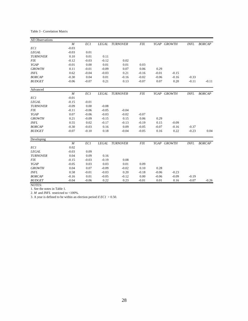
Table 3 presents the sample correlations for the full sample, advanced countries, and

developing countries. Looking at the simple correlations, there does not appear to be a

relationship between election cycles and money growth for either advanced or developing

countries. As we show in Section 3, however, when we control for other variables and consider

the role of CBI, we find that political monetary cycles do exist in developing countries with low

levels of CBI. As expected, the simple correlation between money growth and inflation is large

for both advanced and developing countries. For developing countries, the sign of the

correlation between the two measures of CBI, TURNOVER and LEGAL, is unexpectedly

positive. For advanced countries, the sign of the correlation between money growth and

TURNOVER is unexpectedly negative. As discussed in Cukierman, et al. (1992), LEGAL is not a

good measure of CBI for developing countries, while TURNOVER is not indicative of CBI in

advanced nations. We return to this issue in the results section.

19 We use the TURNOVER measure of CBI rather than the LEGAL measure to divide developing countries since the former is likely to be a better measure of CBI for developing nations.

14

Table 4 presents the summary statistics for developing countries broken up by old and

new democracies (as defined by Brender and Drazen, 2005a) and by election and non-election

periods. For both old and new democracies, average and median budget deficits are larger

during election periods, suggesting the presence of political budget cycles in both. As mentioned

earlier, however, after including the Brender and Drazen (2005a) control variables, we only find

a significant effect of elections on fiscal policy in new democracies. Surprisingly, Table 4

shows a reduction in average and median money growth during elections in new democracies. In

the next section, however, we show that there is no significant change in money growth after

including the control variables.

3. Results on Political Monetary Cycles

Table 5 presents results from the estimation of equation (1). As mentioned above, we

limit observations of money growth and inflation to less than 100%, thus dropping the outliers

from Table 1. This constraint is not binding for advanced economies. We present results for the

full sample, advanced countries, and developing nations using either LEGAL or TURNOVER as

the measure of CBI.

To test for political monetary cycles in the typical economy, we use the coefficients of

EC1 and its interaction terms along with the mean values of the interaction variables. For the

full sample in specification (1), the results imply that political monetary cycles do not exist on

average, regardless of legal independence. In addition, although the coefficient of EC1*LEGAL

has the predicted sign, implying that countries with more legally independent central banks have

less severe political monetary cycles all else equal, this effect is not significant.

15

For the full sample in specification (2), however, the coefficient of EC1*TURNOVER is

positive and significant, implying that countries with higher levels of central bank governor

turnover experience more severe political monetary cycles. In particular, during elections cycles,

M1 growth increases by 10.3 percentage points more in countries with the highest levels of

TURNOVER relative to those with the lowest, all else equal. Further calculations reveal that for

the typical economy, the effect of elections is significantly positive but only for countries with

TURNOVER greater than or equal to 0.32, slightly greater than the average. The size of the

predicted impact on money growth when TURNOVER equals 0.32 is approximately 1.4

percentage points (the VAR analysis in Christiano, et al. (1999) suggests that for the U.S., a one

percentage point increase in M1 growth is associated with an increase in output of 1.5 percentage

points and a 0.6 percentage point increase in inflation after 8 quarters, although these responses

could differ in other countries). This effect increases as TURNOVER increases to a maximum of

8.4 percentage points for a country with TURNOVER equal to one. Thus the effect of elections

on the severity of political monetary cycles in the full sample depends on the level of CBI. This

effect is evident, however, only when we use TURNOVER as our CBI measure. We will explain

shortly why this is the case.

For advanced countries, there is no evidence of political monetary cycles for all values of

LEGAL (specification (3) and TURNOVER (specification (4)). For developing countries

(specification (5)), elections do not significantly increase money growth for any value of

LEGAL. In addition, the coefficient of EC*LEGAL is insignificant, implying that all else equal,

legal independence does not affect political monetary cycles. The results in specification (6),

however, imply that during elections cycles, M1 growth increases by 15.1 percentage points

more in countries with the highest levels of TURNOVER relative to those with the lowest, all

16

else equal. For the typical developing economy, the effect of elections is significantly positive at

the 10% (5%) level but only for countries with TURNOVER greater than or equal to 0.30 (0.34),

slightly greater than the average. This is depicted in Figure 1, which presents the marginal effect

of elections on money growth in developing countries for different values of TURNOVER and

the 90% confidence interval. Thus a significant number of developing countries have

experienced political monetary cycles. The size of the predicted impact on money growth when

TURNOVER equals 0.30 is 1.6 percentage points. This effect grows as TURNOVER increases to

a maximum of 12.2 percentage points when TURNOVER equals one. The coefficients of

TURNOVER and EC1*TURNOVER are jointly significant as is their sum.

As mentioned above, we find evidence of political monetary cycles in the full sample

when we use TURNOVER as our CBI variable, but not when we use LEGAL. LEGAL has no

effect for advanced countries, which for the most part do not experience these cycles, It also has

no effect for developing countries, even though many do experience cycles, presumably because

legal measures of independence are less accurate in developing countries (Cukierman, et al.,

1992). Meanwhile, TURNOVER has a strong effect in developing countries but a smaller and

statistically weaker (although still significant) effect in the full sample. The drop in size and

significance for the full sample can be explained by the fact that some advanced countries have

higher turnover rates than developing countries, but still do not experience political monetary

cycles. Cukierman, et al. (1992) argue that this measure is less indicative of CBI for advanced

countries than the legal measure. In the full sample, the effect of TURNOVER, although weaker,

is still significant. The reason is that advanced countries have lower turnover rates on average

17

and much weaker political monetary cycles than developing countries, while developing

countries with high turnover rates experience larger cycles than those with low turnover rates.20

3.1 Results for the Other Variables

The coefficient of EC1*FIX has the predicted negative sign and is significant but only in

specification (3) for advanced countries. The coefficient of EC1*BORCAP is insignificant in all

specifications.

The coefficient of LEGAL by itself has the expected negative sign but is insignificant,

while the coefficient of TURNOVER has the wrong sign for the full sample and developing

countries. One explanation is that part of the effect of the CBI variables might be captured by

lagged money growth or inflation. Removing both variables increases the size and significance

of LEGAL and TURNOVER (and gives TURNOVER the correct sign). LEGAL, however,

remains insignificant while TURNOVER becomes significant for developing countries.

The coefficient of FIX is negative as expected and close to significant at the 10% level

for developing countries in specification (6). Again the effect could be partially captured by

lagged money growth and inflation. If we remove these variables, the coefficient of FIX equals -

9.6 and is significant at the 1% level for developing countries.

The coefficient of OUTPUTGAP has the predicted negative sign in all specifications and

is significant in specifications (3) and (4), while the coefficient of INFL is unexpectedly positive

and significant. The latter result holds even after excluding LEGAL, TURNOVER, FIX, or M(-1).

This is most likely due to the fact that both money growth and inflation are fairly persistent and

20 This explanation is similar to the one provided in Cukierman, et al. (1992) for why TURNOVER is significant in explaining average inflation for developing countries and for the whole sample, even though it is not significant for industrial countries.

18

highly correlated with each other. If we exclude INFL from the regression, the results for

political monetary cycles are virtually identical.

The coefficient of BORCAP has the predicted negative and significant effect for

advanced countries and for the full sample but not for developing countries. This could result

from greater variation in the development of financial markets among advanced economies.

3.2 Developing Countries in More Detail

In Table 6, we look more closely at the results for developing economies. We show

results with and without restricting money growth observations to less than 100%. In addition,

we present regressions without the interaction terms and control variables. We limit attention to

TURNOVER as a measure of CBI for developing countries since, as previously mentioned, we

find no evidence of political monetary cycles using LEGAL. The most likely explanation is that

legal measures are unlikely to accurately reflect CBI for developing countries.

With the election cycle variable as the sole regressor (apart from lagged money growth),

we find evidence of election cycles only when we do not restrict money growth to less than

100% (specification (2)). The large coefficient of EC1 is mostly likely due to reverse causality

from high inflation episodes to elections. In fact, if we restrict money growth to less than

2000%, the coefficient falls to 9.0 with a p-value of 0.20. If we further restrict money growth to

less than 1000%, the coefficient falls to 0.30 with a p-value of 0.88, results that are very similar

to column (1).

When we add the control variables to the regression that includes the outliers

(specification (4)), this effect disappears. This is not because of the control variables themselves,

but rather because of the reduction in sample size. Specifically, including TURNOVER

19

eliminates some of the highest money growth episodes in the sample since TURNOVER data are

not available for these observations. In fact, if we estimate specification (2) but limit the sample

to data on TURNOVER, the coefficient of EC1 becomes insignificant. Therefore, the sub-sample

of countries and observations with data on TURNOVER do not experience these cycles on

average, regardless of whether money growth is restricted or not.

However, as shown in column (5) (which reproduces column (6) from Table 5), the

impact of elections for these countries does depend on the level of TURNOVER. The restriction

on money growth and inflation has reduced the sample size by 78 observations out of 791. In

column (6), however, the coefficient of EC1*TURNOVER has the right sign but is insignificant.

The fall in significance when we drop the restriction on money growth can be explained by the

presence of just two outliers. The only observations in this regression of money growth greater

than 4000% are Nicaragua in 1988 and Argentina in 1989. Restricting money growth to less

than 4000% yields similar results to column (5), as shown in column (7).

3.3 Robustness Tests

We conduct several tests to check the robustness of our results. First we include year

dummies, two lags of money growth instead of one lag, and both measures of CBI at the same

time. We restrict money growth and inflation to less than 50% as opposed to 100%. We filter

the data using the measure for competitive elections developed in Przeworski et al. (2000) as

opposed to the Freedom House variable.21 None of these modifications change the results

significantly. Second, we include only one year before the election day as the election cycle

21 The authors define democracies as polities in which there are contested elections, i.e. there is some chance that the incumbent executive or party in the legislature is replaced. We therefore limit the regression to democracies. Although the sample size is smaller using this indicator as opposed to the Freedom House variable, the results are similar and are available upon request.

20

indicator (EC2), as opposed to two years. The results are presented in Table 7. In this case, we

do not find evidence of political monetary cycles in both advanced and developing countries,

although the coefficient of EC2*TURNOVER has the predicted positive sign. This is not entirely

surprising given that we may not be capturing the full lag in monetary policy. The VAR analysis

in Christiano, et al.(1999) indicates that the peak in the response of output to a monetary policy

shock is at least a year and often six quarters or more. If monetary policy becomes more

expansionary two years prior to an election, including only one of the years as part of the

election cycle is likely to result in monetary policy that looks similar between election and non-

election periods.

Third, we estimate the model using fixed effects estimation as opposed to GMM,

although in the presence of a lagged dependent variable the fixed effects estimator does not

eliminate dynamic panel bias. While this bias is insignificant for large T, Judson and Owen

(1999) in simulations find a bias of 20% in the coefficient estimate even when T=30, the

maximum number of observations per country in our sample. Moreover, a number of countries

have fewer observations, especially new democracies that have had competitive elections for a

shorter period of time. Results are similar and are available upon request.22

As a fourth robustness test, we include BUDGET, the budget surplus as a percent of

GDP, in our regression. To the extent to which including BUDGET controls for the fiscal-

financing channel, comparing the effect of elections with and without this variable provides

some information about the strength of the fiscal channel. Again, we do not find evidence of

political monetary cycles in advanced countries, and so we only present results for developing

countries. Table 8 presents the results. In columns (1) and (2), we look at the full sample of

22 We use lags of the output gap and inflation to mitigate simultaneity problems when we do fixed effects estimation.

21

developing countries. We continue to limit observations to money growth and inflation of less

than 100%. In column (1) we show the default specification that does not include fiscal policy.

Therefore column (1) presents identical results to column (6) in Table 5. In column (2), we

remove BORCAP and EC1*BORCAP since we include BUDGET.23

A comparison of the columns suggests that controlling for fiscal policy weakens the

effect of elections only slightly. However, this is due solely to the drop in sample size and not

the inclusion of the fiscal variable itself. Specifically, performing the regression in column (1)

but limiting to the observations in column (2) yields similar results to those presented in column

(2). This suggests that the fiscal channel is not strong. In addition, the effect of elections is

significantly positive at the 10% level for countries with TURNOVER greater than 0.40. The fact

that elections still have an impact after controlling for fiscal policy provides some evidence that

elections influence monetary policy through the Phillips curve channel.

We also look at the effect of fiscal policy on political monetary cycles in old and new

democracy observations. Brender and Drazen (2005a) define new democracy observations as

the period that includes the first four competitive elections after a country becomes democratic.

If, as Brender and Drazen (2005a) find and we confirm, political budget cycles occur only in new

democracies, then controlling for fiscal policy should reduce the strength of political monetary

cycles for these countries, but only if the expansionary fiscal policy is monetized. In contrast,

the results for old democracies should be unchanged. In columns (3) and (4), we again look at

developing countries but limit attention to those that are also in the Brender and Drazen (2005)

sample. This reduces the sample size falls from 38 countries to 27. The new and old democracy

23 The coefficient of BUDGET is theoretically ambiguous. Larger budget surpluses require less debt monetization, resulting in a negative coefficient. On the other hand, a central bank might respond to tighter fiscal policy with looser monetary policy, yielding a positive coefficient. Table 8 shows a coefficient that is not significantly different from zero. In addition, if we include the interaction BUDGET*TURNOVER, we do not find that more independent central banks react to fiscal expansions with more contractionary monetary policy than dependent central banks.

22

observations are drawn from this group. Again, the weaker political monetary cycle in column

(4) vs. column (3) is a result of the smaller sample size, not the inclusion of BUDGET.

For new democracy observations, we find no evidence of political monetary cycles even

before controlling for fiscal policy. This suggests that their election-related fiscal expansions are

not monetized and/or that expansionary monetary policy is not needed when fiscal policy is used

instead. For old democracies, the political monetary cycle is a little weaker when we control for

fiscal policy in column (8), although again this is a result of the drop in sample size and not the

inclusion of the fiscal variable itself.24 Therefore, controlling for fiscal policy does not impact

political monetary cycles in old democracies, a result that is consistent with the absence of

political budget cycles in old democracies.

Finally, we consider an additional channel through which elections might affect monetary

policy. If elections cause a rise in political risk in some countries, the central bank might

respond by raising interest rates to prevent capital flight. We therefore interact EC1 with a

measure of political risk. We use the average of Government Stability, Internal Conflict,

External Conflict, and Ethnic Tensions from the International Country Risk Guide. Results were

similar. In addition, eliminating the sudden stop episodes listed in Honig (2008) does not affect

the results.

24 For the mean old democracy observation in column (7), the effect of elections is close to, but never significant at the 10% level. For example, for countries with TURNOVER greater than 0.45, the p-value for the effect of elections is 0.15. Note that even though we do not find a significant impact of elections at the 10% level for both new and old democracies, the impact in the combined sample can still be significant if there are differences between the samples.

23

4. Conclusion

Our first goal in this paper is to expand the analysis of election-induced monetary cycles.

Existing research has not come to a definitive conclusion on the existence of political monetary

cycles in advanced economies. Our results are consistent with studies that have not found a

significant effect. Moreover, we add to the literature by analyzing the role of CBI in developing

economies, where these cycles are more likely to occur. We find evidence of political monetary

cycles in developing countries with low levels of CBI. The findings in this paper, therefore,

underscore the importance of CBI.

Second, we attempt to identify the channels through which elections impact monetary

policy. We find some evidence that political monetary cycles are not caused by monetization of

election-related fiscal expansions, even in new democracies where political budget cycles exist.

This suggests that the Phillips curve channel, i.e. pressure on the central bank to stimulate the

economy in order to increase the probability of re-election, may be an important factor in

generating political monetary cycles.

References Abrams, B. A., and P. Iossifov, 2006, “Does the Fed Contribute to a Political Business Cycle?”

Public Choice, 129:3, 249-262. Agenor, Pierre-Richard, McDermott, C. John, and Prasad, Eswar S. 2000. "Macroeconomic

Fluctuations in Developing Countries: Some Stylized Facts." World Bank Economic Review, 14(2) p. 251-85.

Alesina, A., and N. Roubini, 1992, "Political Cycles in OECD Economies," Review of Economic Studies, 59:4, 663-88.

Alesina, A., Roubini, N., Cohen, G., 1997. Political cycles and the macroeconomy. MIT Press, Cambridge, MA.

Arellano, M., Bond, S., 1991. Some tests of specification for panel data: Monte Carlo evidence and an application to employment equations. Review of Economic Studies 58, 277–297.

Arellano, M. and O. Bover. 1995. Another look at the instrumental variable estimation of error-components models. Journal of Econometrics 68: 29-51.

24

Arnone, Marco, Bernard J. Laurens, Jean-François Segalotto, and Martin Sommer. (2007) “Central Bank Autonomy: Lessons from Global Trends.” IMF Working Paper 07/88.

Beck, Nathaniel, 1987, “Elections and the Fed: Is there a Political Business Cycle,” American Journal of Political Science, 31(1), pp. 194–216.

Blundell, R., and S. Bond. 1998. Initial conditions and moment restrictions in dynamic panel data models. Journal of Econometrics 87: 115-43. Boschen, J. and C. Weise. 2003. “What Starts Inflation: Evidence from the OECD Countries.”

Journal of Money, Credit and Banking. 35(3): 323-349. Brender, A. and A. Drazen. 2005a. “Political budget cycles in new versus established

democracies,” Journal of Monetary Economics 52: 1271–1295. _________ 2005b. "How Do Budget Deficits and Economic Growth Affect Reelection

Prospects? Evidence from a Large Cross-Section of Countries." NBER Working Papers, 11862.

Christiano, L., Eichenbaum, M. and C.L. Evans (1999), “Monetary Policy Shocks: What Have we Learned and to What End?” in J.B. Taylor and M. Woodford (eds), Handbook of Macroeconomics, Volume 1A. pp. 65-148. Amsterdam: Elsevier Science B.V.

Clark, W.R., U.N. Reichert, S.L. Lomas and K.L. Parker. 1998. “International and domestic constraints on political business cycles in OECD economies,” International Organization 51, pp. 87–120.

Crowe, C., and E. Meade. 2007. “The Evolution of Central Bank Governance around the World,” Journal of Economic Perspectives, 21:4, 69-90.

Cukierman, A. and A. H. Meltzer (1986). "A Theory of Ambiguity, Credibility, and Inflation under Discretion and Asymmetric Information," Econometrica, 54(5), pp. 1099-1128.

Cukierman, A., S. Webb, and B. Neyapti. 1992. “Measuring The Independence of Central Banks and Its Effect on Policy Outcomes.” World Bank Economic Review, 6(3): 353–98.

Drazen, A. and M. Eslava (2007), “Electoral Manipulation via Voter-Friendly Spending: Theory and Evidence,” working paper. (Earlier version circulated as NBER Working Paper 11085).

de Haan, J., and D. Zelhorst. 1990. “The impact of government deficits on money growth in developing countries,” Journal of International Money and Finance, 9(4): 455-469.

Dreher, A., Sturm, J.E., and J. de Haan. 2008. Does high inflation cause central bankers to lose their job? Evidence based on a new data set. European Journal of Political Economy 24: 778–787.

Dreher, A., and R. Vaubel. 2004. “Do IMF and IBRD Cause Moral Hazard and Political Business Cycles? Evidence from Panel Data.” Open economies review 15: 5–22.

Fair, Ray, 1978, "The Effect of Economic Events on Votes for President," The Review of Economics and Statistics, 2:159-173.

_________ 1982. “The Effect of Economic Events on Votes for President: 1980 Results,” The Review of Economics and Statistics, May 1982, 322-325. Fischer, S. 1977. "Long-Term Contracts, Rational Expectations, and the Optimal Money Supply

Rule." Journal of Political Economy, 85 (1): 191-205. Franzese, R., 2000. Electoral and Partisan Manipulation of Public Debt in Developed

Democracies, 1956-1990. In R. Strauch and J. von Hagen (eds), Institutions and Fiscal Policy, pp. 61-83. Dordrecht: Kluwer academic press.

Golden, D. G. and J. M. Poterba, 1980, “The Price of Popularity: The Political Business Cycle Re-examined,” American Journal of Political Science, 24: 696-714.

25

Grier, K. B., 1987, “Presidential Elections and Federal Reserve Policy: An Empirical Test,” Southern Economic Journal, 54: 475-96.

Haynes, S. E., and J. A. Stone, 1988, “Does the political business cycle dominate United States unemployment and inflation? In T. Willett, ed., Political business cycles: The economics and politics of stagflation. San Francisco: Pacific Institute.

_________ 1989. “An Integrated Test for Electoral Cycles in the U.S. Economy,” Review of Economics and Statistics, 71:3, 426-34.

Honig, A. 2008. “Do Improvements in Government Quality Necessarily Reduce the Incidence of Costly Sudden Stops?” Journal of Banking & Finance, 32:3, 360-373.

Jácome, L. I., and F. Vázquez. 2005. “Any Link between Legal Central Bank Independence and Inflation? Evidence from Latin America and the Caribbean.” IMF Working paper 75.

Judson, R.A., and A.L. Owen. 1999. Estimating dynamic panel models: A practical guide for macroeconomists Economics Letters 65: 9-15.

Leertouwer, Erik, and Maier, Philipp, 2001, “Who Creates Political Business Cycles: Should Central Banks Be Blamed?” European Journal of Political Economy, 17(3), pp. 445-463.

Lucas, Robert E., Jr. 1972. “Expectations and the Neutrality of Money.” Journal of Economic Theory, 4, 103-l24.

McCallum, B. T., 1978, “The Political Business Cycle: An Empirical Test,” Southern Economic Journal, 44, 504-515.

Nordhaus, W.D., 1975, The political business cycle. Review of Economic Studies 42, 169–190. Persson, T., Tabellini, G., 2003. The Economic Effect of Constitutions: What do the Data Say?

MIT Press,Cambridge, MA. Phelps, E. S. and J. B. Taylor, 1977. “Stabilizing Powers of Monetary Policy under Rational

Expectations,” Journal of Political Economy, 85 (1), 163-190. Przeworski, A., Alvarez, M., Cheibub, J. and Limongi, F. (2000). Democracy and Development:

Political Regimes and Economic Well-being in the World, 1950-1990, New York: Cambridge University Press. Democracy and Development Extended Data Set.

Reinhart, C. and K. Rogoff, 2004, The Modern History of Exchange Rate Arrangements: A Reinterpretation?, Quarterly Journal of Economics 119, 1-48.

Roodman, D. 2006. How to Do xtabond2: An Introduction to "Difference" and "System" GMM in Stata. Working Paper 103. Center for Global Development, Washington. Sachs, Jeffrey. (1987) “The Bolivian Hyperinflation and Stabilization.” American Economic

Review, 77:2, 279-83. Sargent T. (1973). “Rational Expectations, the Real Rate of Interest, and the Natural Rate of

Unemployment,” Brookings Papers on Economic Activity, 1973 (2), 429–72. Correction in BPEA, 1973 (3).

Sargent T. and N. Wallace (1975). “Rational Expectations, the Optimal Monetary Instrument, and the Optimal Money Supply Rule,” Journal of Political Economy, 83 (2), 241–254.

Shi, M., Svensson, J., 2002a. Conditional political budget cycles, CEPR Discussion Paper #3352. _________ (2002b). Political business cycles in developed and developing countries, working

paper, IIES, Stockholm University. Siklos, P., 2008. No Single Definition of Central Bank Independence is Right for All Countries.

Paolo Baffi Centre Research Paper No. 2008-02

26

Table 1: Summary Statistics

All Observations obs. mean median s.d. min. max.M 1,431 53.73 14.01 431.47 -29.62 11,673.40# elections 1,431 0.27 0 0.51 0 2EC1 1,431 0.48 0 0.42 0 1LEGAL 1,144 0.41 0.40 0.17 0.09 0.86TURNOVER 1,146 0.22 0.20 0.18 0.00 1.00FIX 1,431 0.19 0 0.39 0 1YGAP 1,431 0.08 -0.04 3.54 -18.59 17.81GROWTH 1,431 3.55 3.56 3.82 -26.48 19.56INFL 1,430 55.72 8.66 453.78 -7.63 10,205.03BORCAP 1,431 70.46 58.70 48.96 -72.99 311.42BUDGET 1,330 -3.19 -2.83 4.76 -26.74 22.63

Advanced CountriesM 593 11.83 9.86 9.74 -15.93 78.17# elections 593 0.30 0 0.50 0 2EC1 593 0.55 1 0.40 0 1LEGAL 593 0.39 0.34 0.16 0.09 0.73TURNOVER 488 0.16 0.13 0.12 0.00 0.60FIX 593 0.21 0 0.41 0 1YGAP 593 0.00 -0.13 2.55 -8.11 8.66GROWTH 593 3.12 3.03 2.69 -7.28 13.44INFL 592 7.85 5.63 8.22 -1.84 84.22BORCAP 593 90.87 86.60 47.13 14.91 311.42BUDGET 585 -3.35 -2.61 3.87 -15.75 9.12

Developing CountriesM 788 87.96 18.95 579.29 -29.62 11,673.40# elections 788 0.25 0 0.52 0 2EC1 788 0.42 0 0.43 0 1LEGAL 563 0.43 0.43 0.17 0.14 0.86TURNOVER 619 0.26 0.20 0.21 0.00 1.00FIX 788 0.17 0 0.38 0 1YGAP 788 0.11 -0.03 4.17 -18.59 17.81GROWTH 788 3.87 4.21 4.45 -26.48 19.56INFL 788 94.87 11.75 608.62 -7.63 10,205.03BORCAP 788 52.91 41.47 42.40 -72.99 264.17BUDGET 706 -3.29 -3.00 4.98 -26.74 22.63NOTES: 1. Unless otherwise noted, all data are annual. Growth rates and ratios are expressed in percentage terms.The sample period is 1972 to 2001. There are 25 advanced countries and 38 developing countries (63 total).

2. Variable definitions: M = % growth in M1, # elections = the number of election days in a given year (1for one election day and 2 for 2 election days, i.e. multiple elections), EC1 = the default two-year electioncycle indicator. LEGAL = legal measure of CBI (one number per decade with higher numbers indicatinggreater independence), TURNOVER = average number of changes in the central bank governor per year ineach decade (one number per decade with higher numbers indicating less CBI). FIX = 1 for fixed exchangerate regime and 0 otherwise (de facto measure). YGAP = log difference between real GDP and its HP-filtered trend. GROWTH = % growth in real GDP. INFL = CPI inflation rate, BORCAP = borrowingcapacity of the government measured by domestic credit to the private sector as a % of GDP, BUDGET =government budget surplus as a % of GDP.

27

Table 2: Summary Statistics by country type (Advanced vs. Developing), election period, and CBI

Advanced - 25 Countries obs. mean median s.d. min. max.Non-Election Period M 259 11.68 9.81 10.10 -15.93 78.17

YGAP 259 0.15 -0.01 2.58 -8.02 6.96GROWTH 259 3.43 3.20 2.71 -2.92 12.03INFL 259 7.56 4.91 8.83 -1.39 84.22BUDGET 256 -2.93 -2.43 3.55 -13.70 9.12

Election Period M 333 11.96 9.94 9.47 -2.48 65.65YGAP 333 -0.12 -0.18 2.53 -8.11 8.66GROWTH 333 2.88 2.84 2.65 -7.28 13.44INFL 333 8.07 5.88 7.73 -1.84 51.03BUDGET 328 -3.69 -2.83 4.09 -15.75 6.19

Developing - 38 Countries obs. mean median s.d. min. max.Non-Election Period M 404 20.70 17.68 17.11 -24.82 96.23


Election Period M 309 21.30 17.38 17.96 -29.62 94.67YGAP 309 0.37 0.30 3.66 -11.19 11.57GROWTH 309 4.46 4.46 3.98 -10.27 19.56INFL 309 16.97 10.61 17.33 -7.63 98.93BUDGET 279 -3.35 -3.10 4.67 -19.97 21.97

Developing, TURNOVER < 0.31 (high CBI) - 34 countries4 obs. mean median s.d. min. max.Non-Election Period M 311 20.25 17.40 15.69 -8.94 94.90



Developing, TURNOVER >= 0.31 (low CBI) - 17 countries obs. mean median s.d. min. max.Non-Election Period M 93 22.19 18.57 21.20 -24.82 96.23

YGAP 93 -0.52 -0.28 5.62 -18.59 17.81GROWTH 93 3.46 3.91 5.56 -26.48 12.18INFL 93 23.25 13.43 23.47 -0.94 97.00BUDGET 76 -0.60 -1.57 5.15 -7.48 22.63


NOTES:1. See the notes in Table 1. 2. M and INFL restricted to <100%. 3. A year is defined to be within an election period if EC1 > 0.50.4. There are 34 countries that at one point during the sample had TURNOVER < 0.31. Similarly, there are 17 countries that at one point had TURNOVER >= 0.31. The union of these two groups is 38 countries.

28

Table 3 - Correlation Matrix

All ObservationsM EC1 LEGAL TURNOVER FIX YGAP GROWTH INFL BORCAP

EC1 -0.03LEGAL -0.03 0.01TURNOVER 0.10 0.01 0.11FIX -0.12 -0.03 -0.12 0.02YGAP -0.01 0.00 0.01 0.01 0.03GROWTH 0.11 -0.01 -0.09 0.07 0.06 0.29INFL 0.62 -0.04 -0.03 0.21 -0.16 -0.01 -0.15BORCAP -0.30 0.04 0.01 -0.16 -0.02 -0.06 -0.16 -0.33BUDGET -0.06 -0.07 0.21 0.13 -0.07 0.07 0.20 -0.11 -0.11

AdvancedM EC1 LEGAL TURNOVER FIX YGAP GROWTH INFL BORCAP

EC1 -0.01LEGAL -0.15 -0.01TURNOVER -0.09 0.00 -0.08FIX -0.11 -0.06 -0.05 -0.04YGAP 0.07 -0.06 -0.03 -0.02 -0.07GROWTH 0.21 -0.09 -0.15 0.15 0.06 0.29INFL 0.55 0.02 -0.17 -0.13 -0.19 0.15 -0.09BORCAP -0.30 -0.03 0.16 0.09 -0.05 -0.07 -0.16 -0.37BUDGET -0.07 -0.10 0.18 -0.04 -0.05 0.16 0.22 -0.23 0.04

DevelopingM EC1 LEGAL TURNOVER FIX YGAP GROWTH INFL BORCAP

EC1 0.02LEGAL -0.03 0.09TURNOVER 0.04 0.09 0.16FIX -0.15 -0.03 -0.19 0.08YGAP -0.05 0.03 0.03 0.01 0.09GROWTH 0.04 0.07 -0.09 -0.02 0.10 0.28INFL 0.58 -0.01 -0.03 0.20 -0.18 -0.06 -0.23BORCAP -0.16 0.01 -0.05 -0.12 0.00 -0.06 -0.09 -0.19BUDGET -0.04 -0.06 0.22 0.23 -0.01 0.01 0.16 -0.07 -0.26NOTES:1. See the notes in Table 1. 2. M and INFL restricted to <100%. 3. A year is defined to be within an election period if EC1 > 0.50.

29

Table 4: Summary Statistics by country type (new vs. old democracy) and election period

Old Developing Democracy Observations - 24 countries4 obs. mean median s.d. min. max.All Periods M 316 21.16 18.00 16.71 -29.62 96.23

YGAP 316 0.28 0.01 4.19 -18.59 17.81GROWTH 316 3.94 4.40 4.33 -26.48 14.19INFL 316 17.57 11.65 17.55 -7.63 97.00BUDGET 283 -4.06 -3.31 4.18 -23.76 5.26

Non-Election Period M 184 20.81 17.74 17.43 -24.82 96.23YGAP 184 0.28 -0.05 4.56 -18.59 17.81GROWTH 184 3.79 4.41 4.52 -26.48 11.56INFL 184 18.72 11.61 19.56 -0.07 97.00BUDGET 164 -3.59 -2.77 4.00 -23.76 5.26


New Developing Democracy Observations - 19 countriesAll Periods M 203 22.95 19.78 18.68 -20.13 93.58

YGAP 203 0.13 0.11 3.16 -9.44 9.70GROWTH 203 3.57 4.19 3.33 -11.89 12.82INFL 203 20.11 11.44 19.44 -1.17 88.11BUDGET 189 -2.62 -2.31 2.98 -13.02 3.34

Non-Election Period M 103 24.28 21.22 18.14 -9.15 93.58YGAP 103 -0.33 -0.29 3.06 -7.97 7.92GROWTH 103 3.14 3.97 3.63 -11.89 10.63INFL 103 20.47 11.73 19.34 -0.94 75.43BUDGET 96 -2.50 -2.23 2.98 -13.02 2.93


NOTES:1. See the notes in Table 1. 2. M and INFL restricted to <100%. 3. A year is defined to be within an election period if EC1 > 0.50.4. There are 24 developing countries that at one point during the sample were classified as old democracies. Similarly, there are 19 countries that at one point were classified as new democracies. The union of these two groups is 27 countries.

30

Table 5: Equation (1) - GMM Estimation (using EC1 = T-2 years,T)

Dependent variable: M = M1 Growth (%)(1) Full Sample (2) Full Sample (3) Advanced (4) Advanced (5) Developing (6) Developing

EC1 2.465 -2.502 0.880 0.524 3.964 -3.408(2.444) (2.175) (2.049) (2.173) (5.189) (3.306)

M(-1) 0.088 0.041 0.098 0.131 0.065 0.030(0.047)* (0.044) (0.046)** (0.046)*** (0.061) (0.057)

LEGAL -0.385 -2.031 -1.449(3.637) (3.141) (6.099)

TURNOVER -6.155 2.003 -13.294(5.075) (3.259) (7.039)*

FIX -1.078 -2.652 0.335 0.139 -2.360 -3.601(1.484) (1.517)* (1.363) (1.300) (2.297) (2.311)

BORCAP -0.035 -0.042 -0.043 -0.027 -0.025 -0.021(0.016)** (0.016)*** (0.015)*** (0.010)*** (0.023) (0.021)

YGAP -0.157 -0.232 -0.296 -0.376 -0.025 -0.171(0.150) (0.178) (0.135)** (0.198)* (0.226) (0.237)

INFL 0.541 0.484 0.293 0.462 0.642 0.584(0.089)*** (0.103)*** (0.151)* (0.127)*** (0.091)*** (0.103)***

EC1*LEGAL -4.139 -4.546 -5.112(4.309) (3.272) (8.318)

EC1*TURNOVER 10.334 -5.281 15.118(4.899)** (5.296) (7.208)**

EC1*FIX -0.690 2.547 -2.287 -0.759 0.403 5.389(1.721) (2.034) (1.254)* (1.137) (3.483) (4.147)

EC1*BORCAP 0.000 0.001 0.011 0.004 0.000 -0.009(0.014) (0.018) (0.012) (0.012) (0.048) (0.040)

Observations 1,105 1,355 592 642 513 713Countries 60 63 25 25 35 38AR(2) test p-value 0.08 0.36 0.59 0.24 0.18 0.50Hansen J-test p-value 1.00 1.00 1.00 1.00 1.00 1.00NOTES:1. See the notes in Table 1. 2. * significant at 10%; ** significant at 5%; *** significant at 1%.3. Panel regression, 1972-2001, estimated by GMM. Robust standard errors in parentheses. 4. M and INFL restricted to <100%.

31

Table 6: Equation (1) - GMM Estimation (using EC1 = T-2 years,T) - Developing countries with and without M<100%

Dependent variable: M = M1 Growth (%)(1) M <100% (2) (3) M <100% (4) (5) M <100% (6) (7) M <4000%

EC1 -0.046 42.198 1.025 1.205 -3.408 -27.223 -41.798(1.034) (23.811)* (1.014) (12.203) (3.306) (25.130) (19.740)**

M(-1) 0.156 0.223 0.035 -0.154 0.030 -0.155 0.087(0.064)** (0.032)*** (0.056) (0.048)*** (0.057) (0.048)*** (0.054)

TURNOVER -6.001 67.033 -13.294 54.410 1.061(7.175) (41.002) (7.039)* (57.285) (23.303)

FIX -1.519 -5.712 -3.601 -6.852 -5.407(1.394) (4.285) (2.311) (9.532) (5.331)

BORCAP -0.026 0.325 -0.021 0.159 -0.027(0.011)** (0.160)** (0.021) (0.067)** (0.041)

YGAP -0.166 -0.713 -0.171 -0.870 0.861(0.239) (0.634) (0.237) (0.802) (0.866)

INFL 0.562 0.930 0.584 0.931 0.715(0.103)*** (0.041)*** (0.103)*** (0.041)*** (0.156)***

EC1*TURNOVER 15.118 29.968 76.493(7.208)** (54.031) (39.811)*

EC1*FIX 5.389 4.233 6.111(4.147) (17.361) (8.027)

EC1*BORCAP -0.009 0.364 0.379(0.040) (0.290) (0.223)*

Observations 822 905 713 791 713 791 783Countries 38 38 38 38 38 38 38AR(2) test p-value 0.90 0.38 0.48 0.55 0.50 0.54 0.18Hansen J-test p-value 0.70 0.59 1.00 1.00 1.00 1.00 1.00NOTES:1. See the notes in Table 1. 2. * significant at 10%; ** significant at 5%; *** significant at 1%.3. Panel regression, 1972-2001, estimated by GMM. Robust standard errors in parentheses.

32

Table 7: Equation (1) - GMM Estimation (using EC2 = T-1 year,T)

Dependent variable: M = M1 Growth (%)(1) Full Sample (2) Full Sample (3) Advanced (4) Advanced (5) Developing (6) Developing

EC1 1.879 -0.363 1.180 3.651 0.938 -3.232(3.259) (2.039) (3.445) (2.165)* (6.677) (3.655)

M(-1) 0.086 0.046 0.099 0.134 0.070 0.042(0.047)* (0.044) (0.046)** (0.047)*** (0.060) (0.057)

LEGAL -1.108 -4.814 -1.064(2.799) (2.727)* (4.499)

TURNOVER -0.295 2.933 -6.125(4.525) (3.800) (6.093)

FIX -1.496 -2.339 -0.734 -0.589 -2.512 -2.671(1.153) (1.107)** (1.252) (1.221) (1.660) (1.530)*

BORCAP -0.037 -0.044 -0.032 -0.020 -0.041 -0.032(0.015)** (0.013)*** (0.013)** (0.011)* (0.020)** (0.014)**

YGAP -0.157 -0.218 -0.297 -0.368 -0.014 -0.169(0.149) (0.180) (0.132)** (0.192)* (0.222) (0.240)

INFL 0.542 0.469 0.299 0.461 0.624 0.555(0.086)*** (0.103)*** (0.150)** (0.124)*** (0.087)*** (0.104)***

EC1*LEGAL -4.978 0.745 -9.812(5.404) (5.452) (9.457)

EC1*TURNOVER -2.309 -12.855 2.439(7.123) (6.395)** (10.676)

EC1*FIX 0.345 3.265 -0.443 1.082 1.064 5.402(2.359) (2.253) (2.145) (2.178) (4.990) (4.454)

EC1*BORCAP 0.007 0.005 -0.012 -0.013 0.077 0.027(0.017) (0.016) (0.016) (0.018) (0.071) (0.048)

Observations 1,105 1,355 592 642 513 713Countries 60 63 25 25 35 38AR(2) test p-value 0.07 0.38 0.22 0.50 0.17 0.52Hansen J-test p-value 1.00 1.00 1.00 1.00 1.00 1.00NOTES:1. See the notes in Table 1. 2. * significant at 10%; ** significant at 5%; *** significant at 1%.3. Panel regression, 1972-2001, estimated by GMM. Robust standard errors in parentheses. 4. M and INFL restricted to <100%.

33

Table 8: Equation (1) - GMM Estimation (using EC1 = T-2 years,T) - Controlling for fiscal policy

Dependent variable: M = M1 Growth (%)(1) Developing (2) Developing (3) DEV-BD5 (4) DEV-BD (5) New dem. obs. (6) New dem. obs. (7) Old dem. obs. (8) Old dem. obs.

EC1 -3.408 -3.289 -3.159 -4.027 -3.058 -0.969 -6.306 -6.904(3.306) (1.678)* (3.441) (1.866)** (6.085) (5.694) (5.184) (3.295)**

M(-1) 0.030 0.039 0.060 0.111 0.092 0.113 0.016 0.040(0.057) (0.065) (0.064) (0.076) (0.089) (0.087) (0.073) (0.094)

TURNOVER -13.294 -12.363 -11.477 -10.499 -12.389 -12.430 -7.727 -4.479(7.039)* (6.665)* (7.824) (6.681) (7.234)* (8.469) (13.413) (12.241)

FIX -3.601 -2.395 -4.372 -3.140 -2.222 -0.559 -6.538 -5.471(2.311) (2.076) (2.640)* (2.130) (3.449) (3.499) (2.552)** (2.081)***

BORCAP -0.021 -0.019 -0.060 -0.028(0.021) (0.018) (0.029)** (0.020)

BUDGET -0.017 0.024 -0.117 -0.022(0.097) (0.170) (0.381) (0.279)

YGAP -0.171 -0.192 -0.272 -0.376 -0.189 -0.078 -0.311 -0.267(0.237) (0.258) (0.152)* (0.207)* (0.340) (0.327) (0.185)* (0.197)

INFL 0.584 0.504 0.485 0.424 0.541 0.564 0.292 0.177(0.103)*** (0.125)*** (0.099)*** (0.106)*** (0.109)*** (0.103)*** (0.135)** (0.165)

EC1*TURNOVER 15.118 11.793 13.182 10.438 -1.538 -3.225 22.845 17.502(7.208)** (6.138)* (7.636)* (6.502) (22.702) (22.785) (14.148) (11.918)

EC1*FIX 5.389 3.591 6.112 5.463 1.511 0.665 8.026 7.018(4.147) (3.995) (4.684) (4.791) (4.764) (4.513) (5.251) (5.811)

EC1*BORCAP -0.009 -0.016 0.051 -0.014(0.040) (0.039) (0.041) (0.042)

Observations 713 643 519 472 203 189 316 283Countries 38 36 27 27 19 19 24 22AR(2) test p-value 0.50 0.67 0.15 0.31 0.31 0.58 0.18 0.25Hansen J-test p-value 1.00 1.00 1.00 1.00 1.00 1.00 1.00 1.00NOTES:1. See the notes in Table 1. 2. * significant at 10%; ** significant at 5%; *** significant at 1%.3. Panel regression, 1972-2001, estimated by GMM. Robust standard errors in parentheses. 4. M and INFL restricted to <100%. 5. Developing country in the Brender and Drazen (2005) sample.

34

FIG. 1. Marginal Effect of Elections (EC1) on Money Growth (M) in Developing Countries for each level of TURNOVER using specification (6) in Table 5. The dotted lines represent the 90% confidence interval. See the notes in Table 1 for a description of the variables.

0

2

4

6

8

10

15

20

(%)

0 .1 .2 .3 .4 .5 .6 .7 .8 .9 1

TURNOVER

35

Table A1: Variables and Data Sources

Variable Description and SourceM Annual % change in M1. Source: IFS variable 34x.EC1 The default two-year election cycle indicator. Main source - IDEA database.

Additional data sources were used to obtain exact election dates and whether the country has a presidential or parliamentary system. These sources are available upon request.

OUTPUTGAP The log difference between real GDP and its (country specific) trend, estimated using a Hodrick-Prescott filter. GDP is in constant local currency units (WDI).

INFL Annual percent change in consumer price index. Source: WDI.FIX 1 for fixed exchange rate regime and 0 otherwise based on Reinhart and Rogoff

(2004) course classification.BUDGET Central government budget surplus (% of GDP). Source: IFS v80.GROWTH GDP growth (annual %). Source: WDI. NY.GDP.MKTP.KD.ZGBORCAP Domestic credit to private sector (% of GDP): refers to financial resources

provided to the private sector, such as through loans, purchases of nonequity securities, and trade credits and other accounts receivable, that establish a claim for repayment. For some countries these claims include credit to public enterprises. Source: WDI.

TURNOVER TURNOVER is the average number of changes in the central bank governor per year in each decade. For example, if TURNOVER = 0.2, there are 2 changes per decade for an average tenure of 5 years. One observation per decade (1950's to 1980's). Source: Cukierman, et al., (1992). Data after 1990 obtained from Crowe and Meade (2007) and Dreher, et al. (2008).

LEGAL One observation per decade (1950's to 1980's). Source: Cukierman, et al., (1992). Data updated by Jácome and Vázquez (2005) and Siklos (2008).

DEV 0 for advanced, 1 for developing or emerging economy based on the classification in Arnone, et al. (2007).

Political Rights 1 low 7 high. 1972-2005. Source: Freedom House. Civil Liberties 1 low 7 high. 1972-2005. Source: Freedom House. DEM Average of Political Rights and Civil Liberties. Source: Freedom House. reg Przeworski et al. (2000) Democracy and Development Extended Data Set . 1 for

dictatorships, 0 for democracy.

Political Risk Variables Government Stability Source: ICRG published by the PRS group. Ethnic Tensions Source: ICRG published by the PRS group. Internal Conflict Source: ICRG published by the PRS group. External Conflict Source: ICRG published by the PRS group.

Brender and Drazen (2005a) regressorsTRADE Total trade as a % of GDP. Source: WDI. POP1564 Population ages 15-64, % of total. Source: WDI. POP65 Population ages 65 and above, % of total. Source: WDI. GDPPC GDP per capita (constant 2000 $). Source: WDI.

36

Table A2: Countries

Argentina Hungary PakistanAustralia Iceland PanamaAustria India ParaguayBelgium Ireland PeruBolivia Israel PhilippinesBotswana Italy PolandBrazil Jamaica PortugalCanada Japan SingaporeChile Kenya South AfricaColombia Korea SpainCosta Rica Luxembourg SurinameDenmark Malaysia SwedenDominican Republic Malta SwitzerlandEcuador Mexico TanzaniaFinland Morocco ThailandFrance Nepal TurkeyGermany Netherlands United KingdomGhana New Zealand United StatesGreece Nicaragua UruguayGuatemala Nigeria VenezuelaHonduras Norway Zimbabwe

Documents

The impact of central bank independence on political ...and+CBI.pdfThe impact of central bank independence on political monetary cycles in advanced and developing nations* Sami Alpandaa,