http://www.oru.se/Institutioner/Handelshogskolan-vid-Orebro-universitet/Forskning/Publikationer/Working-papers/ Örebro University School of Business 701 82 Örebro SWEDEN

WORKING PAPER

5/2013

ISSN 1403-0586

The impact of extension services on farming households in Western Kenya

– A propensity score approach

Jean-Philippe Deschamps-Laporte

Economics

The impact of extension services on farming households in Western Kenya

A propensity score approach1

Jean-Philippe Deschamps-Laporte2

June 2013

Abstract

The aim of this paper is to assess the impact of the adoption of technological packages in

agriculture Kenya on the farming households, as promoted by the National Agriculture and

Livestock Extension Programme (NALEP), a program run by the Government of Kenya. To this

end, we collected data on beneficiaries through a survey of 1000 households in the district of

Lugari, in Western Kenya. We use propensity score matching to compute the average treatment

effect on the treated. We find evidence that: I) program beneficiaries changed their crop rotation

practices; II) treated households increased their fertilizer dosage by 23.8%; IV) productivity per

acre is not affected by the treatment; V) treated households also were less likely to store their

surplus maize.

JEL Classification: Q16, Q13, Q12

Keywords: Agricultural Extension, Kenya, Propensity Score Matching, Maize, Fertilizer, Crop

Rotation, Productivity

1 We are thankful for the valuable comments and support by the NALEP Permanent Secretariat,

especially to Mikael Segerros. Comments by Jakob Svensson, Gunnar Isacsson, Jörgen Levin and Ranjula

Bali Swain are duly acknowledged. We also thank the seminar participants at the Economics Department

at Örebro University. We are also thankful to NALEP for funding the data collection of this paper. 2 Corresponding author: Economics Department, Örebro Business School, Örebro University, Örebro. E-

mail: jean-philippe.deschamps-laporte@oru.se

1

1. Introduction

Poverty reduction is core to the field of development economics. With 75% of the world’s poor

living in rural areas, the topic of improved agriculture is viewed as central to poverty reduction

(Thirtle, Lin, & Piesse, 2003; de Janvry & Sadoulet, 2010).

Extensive research on agricultural growth since India’s green revolution in the 1960s has

provided evidence on ways to uplift production, livelihoods and food security for the rural poor.

Agricultural productivity gains in India, mainly through the adoption of high yield seeds

varieties (HYV), brought both absolute and relative gains to poor rural households, although

those gains took time to manifest themselves (Ravallion & Datt, 1998). Agricultural extension

services are one of the most common forms of public-sector support for knowledge diffusion

and learning. Extension has the potential of bridging discoveries and mitigation methods from

research laboratories and the in-field practices of individual farmers. In addition to information

about cropping techniques, optimal inputs use, high-yield varieties and prices, extension

frontline agents can improve the managerial skills of farmers by diffusing information on record

keeping, further improving the commercial potential of agricultural production (Birkhaeuser &

Evenson, 1991).

In Kenya, as of 2005, 61% of the population was employed within the agriculture sector (World

Bank, 2013). At the same time, climate change is believed to affect adversely the highly-

productive lands3, representing only 16% of the territory, that are subject to high and medium

rainfalls. Those factors conjugated threaten rural household’s livelihoods, income and food

security. Kenya has suffered from 28 droughts over the last hundred years, four of which have

occurred during the last ten years. Those climatic events threaten the livelihoods and incomes of

the people who depend on agriculture, especially for the country’s poor, who represent a little

over half of the population. In order to act upon the situation, the Government of Kenya has

3 Jones and Thorton (2003) use spatial simulations to predict the effect of climate change on maize

production in Africa and Latin America. They find for Kenya a decrease in maize yields of 6% by 2055,

compared with the yields for the year 2000.

2

introduced the Swedish International Development Agency (Sida) funded4 National Agriculture

and Livestock Extension Programme (NALEP) in the year 2000, which lasted until December

2011. It aimed at uplifting productivity, encouraging commercialization and enhancing

resilience through the increased use of agricultural technologies and improved inputs, using

demand driven and participatory agricultural extension approaches. Whether extension services

contributed to affect technology adoption, crops productivity and incomes in Kenya is the

empirical question studied in this paper. We analyse the average treatment effect on the treated

on outcomes separated in 4 main groups: adoption of extension methods, farm output, revenue,

and basic household welfare. To this end, we use propensity score matching (PSM) to evaluate

the impact of the programme, as first proposed by Rosenbaum and Rubin (1983), using a unique

data set collected for the purpose of this paper.

In terms of relevance, the quantitative impact of technological packages adoption has been

seldom studied, since most of the literature focuses on the impact of the adoption of specific

technologies (Becerril & Abdulai, 2010; Dercon, 2009). This paper distinguishes itself by the

use of data that has been collected in a unique setting in Kenya, by cooperating closely with the

local government. Also, this paper provides a framework for policymakers that enables a

refinement of program evaluation practices.

In a review, Birkhaeuser and Evenson (1991) draw a portrait of agricultural extension since

WWII, underlining the different strengths and weaknesses of the systems. They discuss how the

low level of skills of extension agents sometimes hampered the potential of the different

extension programmes. Other reasons for the failure of extension to enhance productivity

include the lack of understanding of governments on the incentives to adopt new technologies

and whether they suit the socioeconomic and agroecological circumstances of the service

recipients (Anderson & Feder, 2004).

4 The programme benefited from a support of 508M SEK (~80M USD) from Sida, for the whole length of

the programme.

3

Using propensity score matching, as we do in this paper, in order to evaluate program outcomes

is a popular way to proceed, since it offers an alternative for ex-post evaluation, as well as ways

to overcome selection bias. Propensity scores were first used more than three decades ago as a

method to control bias (Cochrane & Rubin, 1973; Rubin, 1973; Rubin, 1979; Bassi, 1984;

Rosenbaum & Rubin, 1985). More recently, its use has been seen a regain in popularity

following works by James Heckman as well as Rajeev Dehejia and Sadek Wahba on the impact

of training programs (Friedlander, Greenberg, & Robins, 1997; Heckman, Ichimura, & Todd,

1997; Heckman, Lalonde, & Smith, 1999; Dehejia & Wahba, 2002; Heckman & Navarro-

Lozano, 2004).

NALEP is seen as a leader in Sub-Saharan Africa (SSA) in terms of coverage and participatory

methods, yet the programme has not generated a great deal of academic research. In 2006, a

Sida report by Cuellar et al. (2006) claimed that 80% of the households part of the program that

formed a producer group – called Common Interest Group (CIG) – stated that the introduction

of the programme has offered new opportunities for men, women and youth in agriculture. The

study revealed that more than 70% of the farmers interviewed claimed that they now regard

agriculture as an enterprise rather than a mean of subsistence. However, the report was mostly

aimed at evaluating the implementation of the program rather than the impact on the livelihoods

and production of program takers and it did, furthermore, not use a formal statistical analysis. A

paper by Richard Githaiga (2007) looked at the impact of CIGs under NALEP. It found that the

CIG approach had a significant impact on farmers’ access to extension services but no

significant impact on farmers’ access to agricultural credit and marketing. In addition, the study

found that CIGs had a significant impact on the agricultural productivity of group members.

Githaiga’s paper suffered from several problems, though. The survey instruments used to collect

the information seem to have been strongly biased towards positive outcomes.

This paper is organized as follows: Section 2 describes the program in length, with information

about the intervention and a specific attention to the types of institutions that were formed under

the program; Section 3 provides information on the data that was collected and a general

4

description of the variables of interest; Section 4 presents the empirical framework on

propensity score matching and the different matching methods employed; in Section 5 we

provide the results and a discussion about them; we then conclude in section 6.

2. The program

The implementation of the National Agriculture and Livestock Extension Programme (NALEP)

started in 2000 and was coordinated jointly by the Ministry of Agriculture and the Ministry of

Livestock Development of Kenya. The programme sought to enhance social economic

development and poverty alleviation through agriculture and livestock development. The

programme generally aimed at providing and facilitating pluralistic and efficient extension

services for increased production, food security, higher incomes and improved environment.

The programme targeted rural populations engaged in agriculture, livestock and fisheries, with a

specific focus on pro-poorness and non-discriminatory access to the program5. NALEP covered

first the high-potential agroecological zones and expanded its coverage in 2007-08 to all

districts in Kenya. NALEP strived to support initiatives at different levels: supporting

institutional set-up (setting up local institutions for improved marketing, lobbying and decision

making, which we describe later), enhancing the use of extension approaches, promoting

technical packages, promoting collaboration and networking with other actors (NGOs, Private

sector, Other Ministries, etc.), mitigating problems associated with gender and other cross-

cutting issues (HIV and AIDS, drugs, alcohol and other substance abuse). This paper focuses on

the direct effects on crops of the adoption of technical packages.

NALEP’s targeting approach was focused on vulnerability and pro-poorness using participatory

methods to identify the needs of beneficiaries. One of the tools used was the Participatory

Analysis of Poverty and Livelihood Dynamics (PAPOLD), a community-driven survey tool

used to identify potential beneficiaries. PAPOLD surveys have been used in several agricultural

and forestry projects that used participatory approaches in Burkina Faso, Vietnam and Kenya

5 By this, we mean that the program took affirmative action in selection poor, vulnerable and excluded

individuals.

5

(Hoang & Nguyen, 2011). The survey was performed at the beginning of the implementation

period in each sub-location6 where NALEP was about to deliver services. It included a census of

the sub-location’s dwellings and an asset-scale wealth chart 7 , and other location specific

agricultural information on soils, production, etc. The PAPOLD survey’s goal was twofold:

identifying the needs of vulnerable households to accessing resources for productivity, and

assisting the farmers 8 to commercialize their products. NALEP’s mandate was to deliver

services to all divisions in Kenya, even though it has not been achieved fully by the end of the

programme. Hence, there was no formal “selection mechanism” that assigned treatment to a

sub-location, but rather a progressive roll-out of the programme to the whole country’s

divisions. The decision making process that determined which division received the

programme’s support first is formally stated in the programme procedure and could not be

determined accurately.

NALEP was operationalized through a structure composed of grass-root institutions. The

highest level of institution that was created through NALEP was the stakeholders’ forum (SHF),

with representation from both the public and private sectors, formed the entry point for NALEP

in a new treatment area9, called focal area by the programme. The stakeholders included private

extension service providers, input suppliers, marketing agents, NGOs, community based

organizations (CBOs), government ministries and departments, local councils and other

development structures. The SHF was responsible for conducting a Broad Based Survey (BBS)

6 The lowest agglomeration is called the Sub-location, which is the equivalent of a small village.

Municipalities often encompass several locations. The sub-location is superseded by the Location, the

Division, the District and the Province. 7 The community, through communal meetings (barazas), had to decide on the asset scale and the

relevant thresholds for poverty. E.g. If a household owned kitchen utensils, it is not considered very poor;

if a household owned a bicycle, it is not considered poor. Then, using the list of households that were

considered poor and very poor, extension services were designed according to the needs of the sub-

location. 8 NALEP did not provide assistance to large scale farmers or to the ones possessing modern technologies,

such as mechanic farming tools. 9 Typically 300 ha and 2000 households per focal area per year. The focal area covered a subset of a

location. Those focal areas shall in principle be interacting with NALEP for 3 years, but in practice, due

to logistical constraints, the time spent in a focal area was a year.

6

– a sort of baseline10, in the focal area with the assistance of NALEP technical personnel ending

with the production of a Community Action Plan (CAP) defining the community’s own projects

– a type of “community business plan”. Rather than imposing solutions to the households,

NALEP mobilised communities to generate their own projects and to link them with

development agencies to facilitate implementation of the projects. The community was in

charge of project cycle management and ownership of all community development projects, in

order to facilitate the phasing out process and avoid the “aid void”.

One level below the SHF, NALEP helped developing the Focal Area Development Committee

(FADC), which was a committee formed for the purposes of steering and coordinating

collaborative activities of the focal area. It played the role of an indigenous commerce chamber.

Among the FADC, NALEP encouraged individuals to work together and to form Common

Interest Groups (CIGs). A CIG is a group of individuals that have come together to develop a

commodity (in either livestock or crop production) or activity into a commercial enterprise with

marketing as a major thrust. It is a kind of cooperative, although lacking the level of formality

of a proper cooperative. Through these groups, NALEP contributed in building local capacities

in various technical areas, rights of farmers, pastoralists, fisher folk, and other clients and

mainstreaming gender and other cross-cutting11 issues.

CIGs provided a platform for bargaining, as well as for extension service provision in general.

Although the type of extension programme called “training and visit” (T&V) programs –

usually one-on-one sessions – have met quite a degree of success elsewhere, showing high

returns on investment from the point of view of the program (Bindlish & Evenson, 1997),

NALEP found it more cost effective to collaborate with groups rather than with individuals. The

group approach also allows for the infusion of leadership capabilities among members of the

community, as they rotate group leadership positions.

10 The BBS was not performed with the aim of evaluating the program. The quality of the data was poor

and its availability was scarce. 11 In aid, cross-cutting issues are viewed as supporting conditions for development. They include

mitigating problems linked to substance abuse, health, violence, etc.

7

The decline of central planning, combined with a growing concern for sustainability and equity,

has resulted in participatory methods gradually replacing top-down approaches in extension that

were used in former programmes.

3. Data

In February 2012, we sampled 1000 household using a household survey in the district of

Lugari over 25 consecutive days. We designed the survey based on publicly available

documentation and the specific nature of the programme. 10 enumerators have been trained for

the purpose of the data collection, which we supervised directly with the support of the NALEP

staff based in Lugari. That region has been selected with the support of various agronomic

experts and managers at NALEP headquarters in Nairobi, in order to represent a core region

where NALEP was active, the high-potential region. Within the Lugari district, a treatment and

control group have been selected, upon analysis of internal documentation of the programme.

The control group needed to exhibit the same characteristics (ethnic composition, soil quality,

average education level, rainfall, etc.) as the treatment group, upon assessment of the

programme staff and data from the Kenya National Bureau of Statistics. The data has been

collected in 2 distinct locations, 500 surveys by location, but all within the Lugari district. The

treated region was represented by the Lugari sub-location part of the Lugari location, while the

control region was surveyed in the Chekalini Location, divided between the Musembe and

Koromaiti sub-locations. Figure A.3 and Figure A.4 in appendix detail the specific location of

the survey. Each survey location was assigned to a sub-group of enumerators who divided the

territory in quadrants and proceeded to a random walk survey selection process. The control and

the treatment survey areas are adjacent to each other, yet the villages used for the sampling are

located at the extreme south border of the Chekalini location, in order to try to avoid spill-overs.

The border between the two locations is delimited by the administrative town of Lugari,

meaning that both sampled and control regions are located at equal distance from the main

market of the whole district. A small river had confluents that spread equally to both location

and road access to Lugari town was of similar (low) quality among the sampled locations.

8

After cleaning the dataset, as certain households interviewed were not farming or only raising

livestock (27 households), or that the surveys were not fully completed or the quality of certain

enumerator’s work was not acceptable12, a total of 665 survey remained. Further analysis of the

data led to the conclusion that either a small part of the respondents exaggerated certain reported

values or that mistakes in the data input led to faulty numbers. Therefore, there was a need to

adjust for outliers. We decided to proceed to trimming the yields and prices at 5%, which led to

reasonable upper and lower boundaries, given publicly available data on crops yields and prices.

Ethnic diversity was not a suitable piece of information13 to be collected, and information on

soil quality could not be collected in this study, due to logistical limitations14. The survey was

composed of 115 questions and was divided in 5 categories: demographics, household

characteristics (assets, energy, expenditures, water, sanitation and hygiene), health (access,

HIV/AIDS, prevalence of diseases, mortality), agriculture and livestock (productivity,

production, use of inputs, prices, income and extension services and other income generating

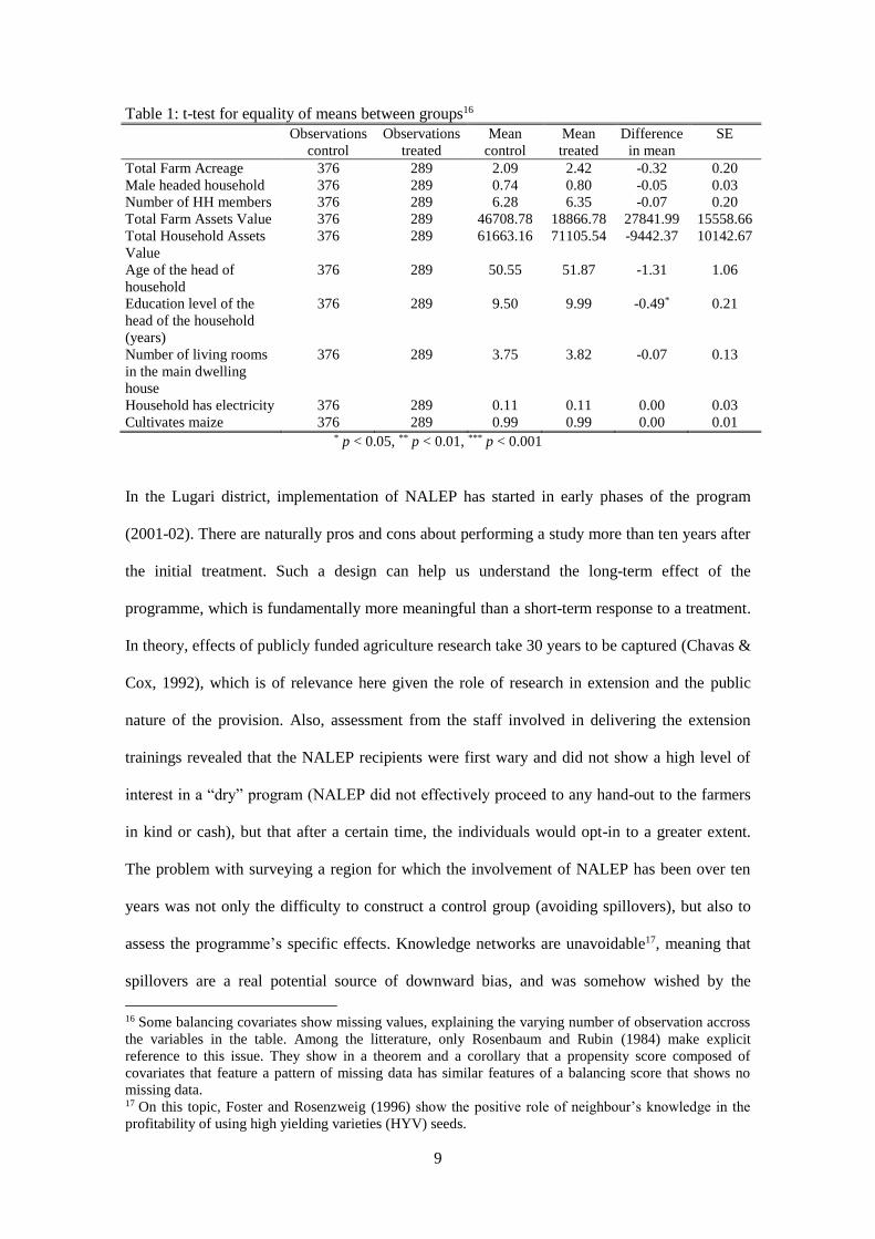
activities) and food security,. Table 1 below presents the results of the test for the difference in

means between treated and non-treated households15, over a set of control variables. In general,

we observe that the control and treatment are rather similar, with education years of the head of

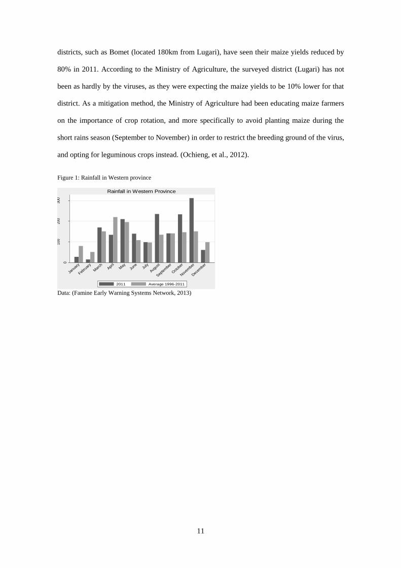
the household being slightly higher for the treated group (+0.5 year). Table 2 also presents the

unmatched effect of the program on a set of outcome variables.

12 One enumerator was suspected to have falsified the data; hence all of his work was discarded (100

surveys). 13 The information was deemed too sensitive to be collected, as Kenya has a long history of social

tensions between ethnic groups. Moreover, the very concept of tribal ethnicity as a binary variable can be

seen as a social construction. 14 Otherwise available data was not detailed enough to include soil quality as a control variable. 15 The variables presented in Table 1 are used later in this paper in order to construct the propensity

scores. The t-test results are presented here in order to describe the differences between the treated and

control group on variables that are assumed not to be affected by treatment.

9

Table 1: t-test for equality of means between groups16

Observations

control

Observations

treated

Mean

control

Mean

treated

Difference

in mean

SE

Total Farm Acreage 376 289 2.09 2.42 -0.32 0.20

Male headed household 376 289 0.74 0.80 -0.05 0.03

Number of HH members 376 289 6.28 6.35 -0.07 0.20

Total Farm Assets Value 376 289 46708.78 18866.78 27841.99 15558.66

Total Household Assets

Value

376 289 61663.16 71105.54 -9442.37 10142.67

Age of the head of

household

376 289 50.55 51.87 -1.31 1.06

Education level of the

head of the household

(years)

376 289 9.50 9.99 -0.49* 0.21

Number of living rooms

in the main dwelling

house

376 289 3.75 3.82 -0.07 0.13

Household has electricity 376 289 0.11 0.11 0.00 0.03

Cultivates maize 376 289 0.99 0.99 0.00 0.01 * p < 0.05, ** p < 0.01, *** p < 0.001

In the Lugari district, implementation of NALEP has started in early phases of the program

(2001-02). There are naturally pros and cons about performing a study more than ten years after

the initial treatment. Such a design can help us understand the long-term effect of the

programme, which is fundamentally more meaningful than a short-term response to a treatment.

In theory, effects of publicly funded agriculture research take 30 years to be captured (Chavas &

Cox, 1992), which is of relevance here given the role of research in extension and the public

nature of the provision. Also, assessment from the staff involved in delivering the extension

trainings revealed that the NALEP recipients were first wary and did not show a high level of

interest in a “dry” program (NALEP did not effectively proceed to any hand-out to the farmers

in kind or cash), but that after a certain time, the individuals would opt-in to a greater extent.

The problem with surveying a region for which the involvement of NALEP has been over ten

years was not only the difficulty to construct a control group (avoiding spillovers), but also to

assess the programme’s specific effects. Knowledge networks are unavoidable17, meaning that

spillovers are a real potential source of downward bias, and was somehow wished by the

16 Some balancing covariates show missing values, explaining the varying number of observation accross

the variables in the table. Among the litterature, only Rosenbaum and Rubin (1984) make explicit

reference to this issue. They show in a theorem and a corollary that a propensity score composed of

covariates that feature a pattern of missing data has similar features of a balancing score that shows no

missing data. 17 On this topic, Foster and Rosenzweig (1996) show the positive role of neighbour’s knowledge in the

profitability of using high yielding varieties (HYV) seeds.

10

program. The obvious disadvantage of such a setting is that other factors might have influenced

welfare and productivity over the course of the period, other than the treatment, since the

treatment is clustered at the sub-location level. This nonetheless remains a potential source of

bias that appears unavoidable in our setting, which we discuss later in this paper. The advantage

of investigating the long-run effect is that it addresses a key objective of the program:

improving livelihoods through demand-led increase in sustainable production. The goal of the

program was indeed not to improve livelihoods and productions for the time of the intervention,

but rather to create a long-lasting effect18.

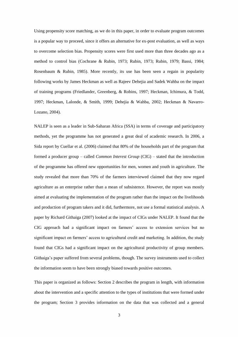
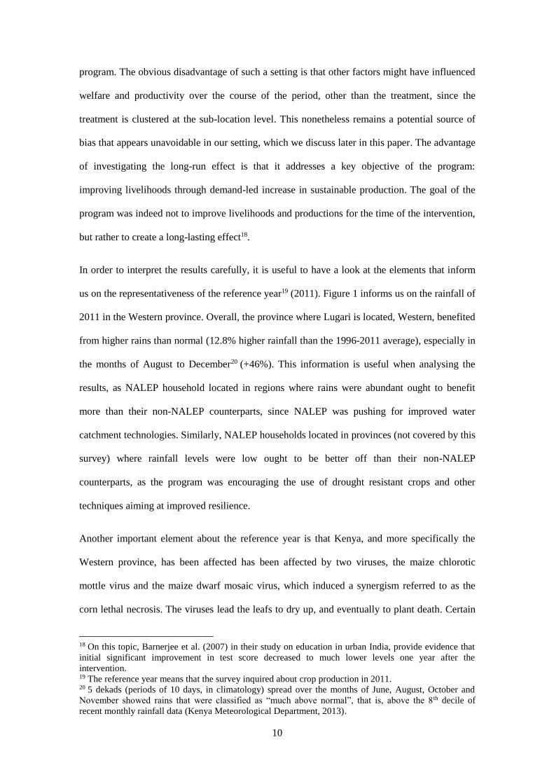
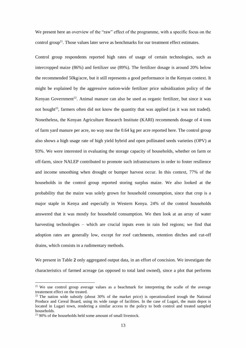
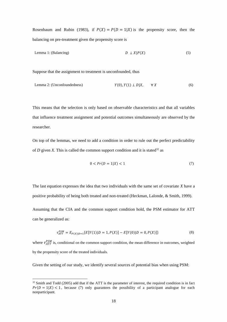
In order to interpret the results carefully, it is useful to have a look at the elements that inform

us on the representativeness of the reference year19 (2011). Figure 1 informs us on the rainfall of

2011 in the Western province. Overall, the province where Lugari is located, Western, benefited

from higher rains than normal (12.8% higher rainfall than the 1996-2011 average), especially in

the months of August to December20 (+46%). This information is useful when analysing the

results, as NALEP household located in regions where rains were abundant ought to benefit

more than their non-NALEP counterparts, since NALEP was pushing for improved water

catchment technologies. Similarly, NALEP households located in provinces (not covered by this

survey) where rainfall levels were low ought to be better off than their non-NALEP

counterparts, as the program was encouraging the use of drought resistant crops and other

techniques aiming at improved resilience.

Another important element about the reference year is that Kenya, and more specifically the

Western province, has been affected has been affected by two viruses, the maize chlorotic

mottle virus and the maize dwarf mosaic virus, which induced a synergism referred to as the

corn lethal necrosis. The viruses lead the leafs to dry up, and eventually to plant death. Certain

18 On this topic, Barnerjee et al. (2007) in their study on education in urban India, provide evidence that

initial significant improvement in test score decreased to much lower levels one year after the

intervention. 19 The reference year means that the survey inquired about crop production in 2011. 20 5 dekads (periods of 10 days, in climatology) spread over the months of June, August, October and

November showed rains that were classified as “much above normal”, that is, above the 8th decile of

recent monthly rainfall data (Kenya Meteorological Department, 2013).

11

districts, such as Bomet (located 180km from Lugari), have seen their maize yields reduced by

80% in 2011. According to the Ministry of Agriculture, the surveyed district (Lugari) has not

been as hardly by the viruses, as they were expecting the maize yields to be 10% lower for that

district. As a mitigation method, the Ministry of Agriculture had been educating maize farmers

on the importance of crop rotation, and more specifically to avoid planting maize during the

short rains season (September to November) in order to restrict the breeding ground of the virus,

and opting for leguminous crops instead. (Ochieng, et al., 2012).

Figure 1: Rainfall in Western province

Data: (Famine Early Warning Systems Network, 2013)

0

10

02

00

30

0

Ra

infa

ll (m

m.)

Janua

ry

Febru

ary

Mar

chApr

ilM

ayJu

neJu

ly

Augus

t

Septe

mbe

r

Oct

ober

Nove

mber

Dece

mber

Rainfall in Western Province

2011 Average 1996-2011

12

Table 2: t-test for equality of means between groups, outcome variables

Observation

s control

Observation

s treated

Mean

control

Mean

treated

Difference

in mean

SE

Extension

Intercropped maize‡ 358 285 0.86 0.91 -0.05 0.02

Use of fertilizer‡ 343 287 0.89 0.90 -0.01 0.02

Fertilizer dosage per

acre (Kg/a)

288 203 40.81 50.70 -9.89* 3.98

Use of farm yard

manure‡

340 279 0.64 0.70 -0.06 0.04

Manure dosage per

acre (Kg/a)

340 279 0.47 0.55 -0.08 0.06

Use of hybrid/OPV

seeds‡

344 281 0.93 0.90 0.03 0.04

Surplus maize was

stored‡

343 285 0.77 0.62 0.14*** 0.04

Maize for HH

consumption‡

364 289 0.24 0.26 -0.02 0.03

Use of retention

ditches‡

354 288 0.19 0.20 -0.02 0.03

Use of water pans‡ 354 288 0.03 0.08 -0.05** 0.02

Use of cut-off drains‡ 353 288 0.29 0.24 0.05 0.03

Use of dams‡ 354 287 0.01 0.00 0.01 0.00

Use of waterholes‡ 354 288 0.11 0.11 -0.00 0.03

Use of irrigation

canals‡

354 288 0.13 0.13 -0.00 0.03

Use of roof

catchments‡

353 288 0.55 0.49 0.06 0.04

Output

Total farmed acreage 364 289 3.60 5.25 -1.64*** 0.45

Total nominal yield

(kg)

364 289 1080.15 1250.11 -169.95 105.23

Total yield per acre

(kg/a)

362 285 358.18 328.52 29.66 38.88

Revenue

Total gross revenue

(Ksh)

364 289 29253.08 33393.44 -4140.36 2503.79

Total revenue per acre

(Ksh/a)

362 285 9883.29 8570.27 1313.02 760.87

Welfare

Monthly HH

expenditure (Ksh)

198 189 14739.38 19060.02 -4320.64** 1620.14

HH Expenditure per

capita (Ksh)

198 189 2598.72 3093.39 -494.67 271.81

Below the extreme

poverty line‡

364 289 0.44 0.38 0.06 0.04

Below the extreme

poverty line‡

364 289 0.26 0.21 0.06 0.03

Faced hunger in 2011‡ 362 287 0.73 0.74 -0.01 0.04

Hungry spell length 254 206 4.76 4.22 0.53*** 0.15 * p < 0.05, ** p < 0.01, *** p < 0.001, ‡ Yes = 1

13

We present here an overview of the “raw” effect of the programme, with a specific focus on the

control group21. Those values later serve as benchmarks for our treatment effect estimates.

Control group respondents reported high rates of usage of certain technologies, such as

intercropped maize (86%) and fertilizer use (89%). The fertilizer dosage is around 20% below

the recommended 50kg/acre, but it still represents a good performance in the Kenyan context. It

might be explained by the aggressive nation-wide fertilizer price subsidization policy of the

Kenyan Government22. Animal manure can also be used as organic fertilizer, but since it was

not bought23, farmers often did not know the quantity that was applied (as it was not traded).

Nonetheless, the Kenyan Agriculture Research Institute (KARI) recommends dosage of 4 tons

of farm yard manure per acre, no way near the 0.64 kg per acre reported here. The control group

also shows a high usage rate of high yield hybrid and open pollinated seeds varieties (OPV) at

93%. We were interested in evaluating the storage capacity of households, whether on farm or

off-farm, since NALEP contributed to promote such infrastructures in order to foster resilience

and income smoothing when drought or bumper harvest occur. In this context, 77% of the

households in the control group reported storing surplus maize. We also looked at the

probability that the maize was solely grown for household consumption, since that crop is a

major staple in Kenya and especially in Western Kenya. 24% of the control households

answered that it was mostly for household consumption. We then look at an array of water

harvesting technologies – which are crucial inputs even in rain fed regions; we find that

adoption rates are generally low, except for roof catchments, retention ditches and cut-off

drains, which consists in a rudimentary methods.

We present in Table 2 only aggregated output data, in an effort of concision. We investigate the

characteristics of farmed acreage (as opposed to total land owned), since a plot that performs

21 We use control group average values as a beachmark for interpreting the scalle of the average

treatement effect on the treated. 22 The nation wide subsidy (about 30% of the market price) is operationalized trough the National

Produce and Cereal Board, using its wide range of facilities. In the case of Lugari, the main depot is

located in Lugari town, rendering a similar access to the policy to both control and treated sampled

households. 23 90% of the households held some amount of small livestock.

14

crop rotation will show a higher yearly acreage. Control households use on a yearly basis 3.60

acre, which generate 1.08 ton of aggregate crop output24. The unit-level yield per acre average

corresponds to 358 kg per acre. Those crops generated a gross revenue for the control group of

29 253 Ksh per year, which relates to an average unti-level gross crop revenue per acre of

9 883 Ksh.

Using an aggregation of 19 expenditure item categories25, we evaluated monthly household

expenditures. It is common practice to use expenditures to evaluate income using expenditure,

since it has a tendency to reflect a smooth income and avoids problems associated with recall

bias (Atkinson & Bourguignon, 2000). That monthly figure amounted to roughly 14 700 Ksh

(176 USD)26, which corresponds to around 2 600 Ksh per capita (31 USD). Using the national

poverty and extreme poverty lines27, we created binary variables for poverty. The poverty rate in

the control group (44%) corresponds roughly to the rate for Lugari made available by the

Government of Kenya (47%). We have also included a more subjective outcome variable on

food security, where the respondents were asked whether they faced hunger in the year previous

to the survey. If so, they were then asked on the duration of that spell. Those last two outcome

variables are more problematic to use, since they are highly subjective28. It is also probable that

the treatment influences the way households perceive and define food insecurity. Also,

assessment from the survey enumerators revealed that households were sometimes expecting

interventions in their communities if their needs appeared urgent. Nonetheless, we decided to

include those variables. Figures on food insecurity are much higher for 2011 at 73%, a potential

24 The aggregate comprises output of the most common crops in Lugari : Maize, beans, sweet potatoes,

sorghum, millet, kales, grain amaranth and sunflower. 25 Those items include: Rent, school fees, food items, health care, energy (coal, wood, electricity, etc.),

water, clothing, transport, telecommunication, domestic workers, bank repayments, savings payments,

transfers, loans, purchases of land and other contributions. Figures were sometimes provided in yearly

figures (i.e. school fees) and were adjusted to a monthly basis. 26 1 USD = 83.40 KSH, rate of February 1st 2012 27 The indexed rural extreme poverty line corresponds to the theoretical rural extreme poverty threshold

of Ksh 1 228 per month per adult equivalent. The rural poverty line is set at Ksh 1942 per month per adult

equivalent. The national poverty line was last made available in 2005, we indexed if to February 2012

using CPI data from the Kenya National Bureau of Statistics. 28 One could consider, for instance, that the treatment influences the way households perceive the very

definition of food insecurity.

15

consequence of the drought and the destroyed crops in the second half of 2010, whereas the

length of that spell was on average of 4.76 months, or 148 days.

4. Empirical approach

This study uses non-parametric propensity score matching (PSM) methods in order to estimate

the effect of the treatment, which here refers to participating in the programme. This technique

first introduced by Rosenbaum and Rubin (1983), involves pairing individuals among two

groups, treated and control, using a large set of information on those individuals29. PSM is a

popular method to evaluate the impact of economic policies on individuals or households

(Lechner, 2002; Jalan & Ravallion, 2003).

An important issue that needs to be overcome using this strategy is how to ensure that selection

problems do not bias the result. The challenge here is to reconstruct a control group that has the

same observable characteristics as the treated group. PSM pairs individuals in a treated group

(like households participating in NALEP) to individuals in an untreated group (like households

not participating in NALEP) using a large set of observable information and assuming that the

outcomes are independent of assignment to treatment, conditional on pre-treatment covariates,

the method can lead to unbiased estimators of the treatment impact (Dehijia & Wahba, 2002).

This technique is widely acknowledged (Heckman, Ichimura, & Todd, 1997; Dehejia & Wahba,

2002; Heckman & Navarro-Lozano, 2004) to produce unbiased results when the assumptions

are respected.

Since no consistent baseline information was collected by the program, longitudinal techniques,

such as Difference-in-Difference could not be used. The assignment rule of the treatment was

not strict – it was based on an asset-scale that was locally established in each PAPOLD, and the

roll-out assignment of the extension treatment has not been randomly assigned. Clearly, those

issues restricted the analytical tools available to assess impacts of the programme. One option

would have been to proceed with a simple linear regression with treatment as a control, but

29 For an overview, Caliendo & Kopeinig (2005) provide a survey of the methodologies.

16

obvious problems related to selection would have arisen. Instead, we opted for the method of

propensity score matching. Angrist and Pischke (2008) also argue that matching and regression

are not that different, after all, up until the point when we specify a model for the score. That

specification is, according to them, analogous to the problem of parametrization of the control

variables in regression settings. They also add that PSM focuses researcher attention on models

for treatment assignment, instead of the typically more complex and mysterious process

determining outcomes, which is well suited for cases where treatment assignment is the product

of human institutions or government regulations.

The impact of the intervention needs to be separated from what would have happened anyway

to the individuals without the presence of the intervention, the so called counter factual. In order

to do this, the observed outcomes need to be differentiated from individuals who were affected

by the treatment and the counterfactual potential outcome, had the same individual been

observable with and without treatment. This is obviously impossible, but the potential outcome

𝑌𝑖(𝐷𝑖) for each individual i, where 𝑖 = 1, … , 𝑁 and N denotes the total population, is

represented below in Eq. (1), where 𝑌𝑖(1) is the outcome for the treated individual i and 𝑌𝑖(0) is

the outcome for the non-treated individual.

𝜏𝑖 = 𝑌𝑖(1) − 𝑌𝑖(0) (1)

Clearly, 𝜏𝑖 cannot be observed, since an individual is either treated or not, so we focus instead

on average population effects.

The parameter of interest is the average treatment effect on the treated (ATT)30, defined as:

𝜏𝐴𝑇𝑇 = 𝐸[𝜏|𝐷 = 1] = 𝐸[𝑌(1)|𝐷 = 1] − 𝐸[𝑌(0)|𝐷 = 1] (2)

30 Another parameter of interest could have been the average treatment effect (ATE), 𝜏𝐴𝑇𝐸 =𝐸[𝑌(1) − 𝑌(0)], but this parameter causes problems, since both counterfactuals have to be reconstructed,

that is, 𝐸[𝑌(1)|𝐷 = 0] and 𝐸[𝑌(0)|𝐷 = 0]. Most of the literature focuses on ATT.

17

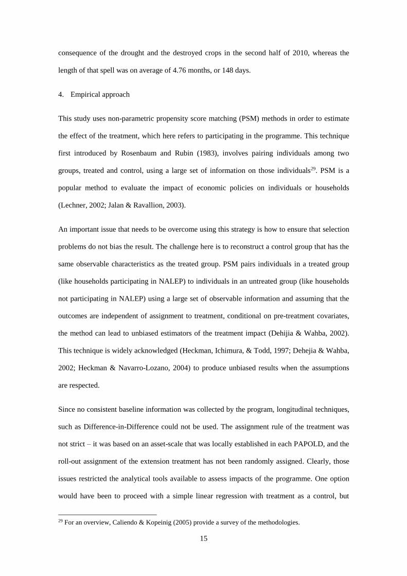
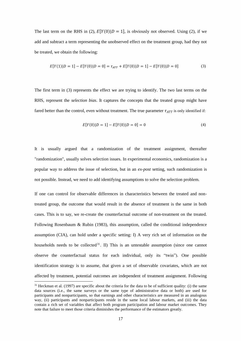
The last term on the RHS in (2), 𝐸[𝑌(0)|𝐷 = 1], is obviously not observed. Using (2), if we

add and subtract a term representing the unobserved effect on the treatment group, had they not

be treated, we obtain the following:

𝐸[𝑌(1)|𝐷 = 1] − 𝐸[𝑌(0)|𝐷 = 0] = 𝜏𝐴𝑇𝑇 + 𝐸[𝑌(0)|𝐷 = 1] − 𝐸[𝑌(0)|𝐷 = 0] (3)

The first term in (3) represents the effect we are trying to identify. The two last terms on the

RHS, represent the selection bias. It captures the concepts that the treated group might have

fared better than the control, even without treatment. The true parameter 𝜏𝐴𝑇𝑇 is only identified if:

𝐸[𝑌(0)|𝐷 = 1] − 𝐸[𝑌(0)|𝐷 = 0] = 0 (4)

It is usually argued that a randomization of the treatment assignment, thereafter

"randomization", usually solves selection issues. In experimental economics, randomization is a

popular way to address the issue of selection, but in an ex-post setting, such randomization is

not possible. Instead, we need to add identifying assumptions to solve the selection problem.

If one can control for observable differences in characteristics between the treated and non-

treated group, the outcome that would result in the absence of treatment is the same in both

cases. This is to say, we re-create the counterfactual outcome of non-treatment on the treated.

Following Rosenbaum & Rubin (1983), this assumption, called the conditional independence

assumption (CIA), can hold under a specific setting: I) A very rich set of information on the

households needs to be collected31. II) This is an untestable assumption (since one cannot

observe the counterfactual status for each individual, only its “twin”). One possible

identification strategy is to assume, that given a set of observable covariates, which are not

affected by treatment, potential outcomes are independent of treatment assignment. Following

31 Heckman et al. (1997) are specific about the criteria for the data to be of sufficient quality: (i) the same

data sources (i.e., the same surveys or the same type of administrative data or both) are used for

participants and nonparticipants, so that earnings and other characteristics are measured in an analogous

way, (ii) participants and nonparticipants reside in the same local labour markets, and (iii) the data

contain a rich set of variables that affect both program participation and labour market outcomes. They

note that failure to meet those criteria diminishes the performance of the estimators greatly.

18

Rosenbaum and Rubin (1983), if 𝑃(𝑋) = 𝑃(𝐷 = 1|𝑋) is the propensity score, then the

balancing on pre-treatment given the propensity score is

Lemma 1: (Balancing) 𝐷 ⊥ 𝑋|𝑃(𝑋) (5)

Suppose that the assignment to treatment is unconfounded, thus

Lemma 2: (Unconfoundedness) 𝑌(0), 𝑌(1) ⊥ 𝐷|𝑋, ∀ 𝑋 (6)

This means that the selection is only based on observable characteristics and that all variables

that influence treatment assignment and potential outcomes simultaneously are observed by the

researcher.

On top of the lemmas, we need to add a condition in order to rule out the perfect predictability

of D given X. This is called the common support condition and it is stated32 as

0 < 𝑃𝑟(𝐷 = 1|𝑋) < 1 (7)

The last equation expresses the idea that two individuals with the same set of covariate X have a

positive probability of being both treated and non-treated (Heckman, Lalonde, & Smith, 1999).

Assuming that the CIA and the common support condition hold, the PSM estimator for ATT

can be generalized as:

𝜏𝐴𝑇𝑇𝑃𝑆𝑀 = 𝐸𝑃(𝑋)|𝐷=1{𝐸[𝑌(1)|𝐷 = 1, 𝑃(𝑋)] − 𝐸[𝑌(0)|𝐷 = 0, 𝑃(𝑋)]} (8)

where 𝜏𝐴𝑇𝑇𝑃𝑆𝑀 is, conditional on the common support condition, the mean difference in outcomes, weighted

by the propensity score of the treated individuals.

Given the setting of our study, we identify several sources of potential bias when using PSM:

32 Smith and Todd (2005) add that if the ATT is the parameter of interest, the required condition is in fact

𝑃𝑟(𝐷 = 1|𝑋) < 1 , because (7) only guarantees the possibility of a participant analogue for each

nonparticipant.

19

Bias 1. Spillovers. A major problem with development programs is the “aid void”: once the

involvement of the donor/government/NGO is over, the initiatives die out. NALEP has

deployed extensive efforts to enhance leadership capacities in the communities, for them to

maintain the extension technologies and to share them among producers. Such “knowledge

networks” are not necessarily community bound, meaning that with better roads and

telecommunication, knowledge is likely to spread further than ever. This represents a great

achievement of development projects – to enhance indigenous institutions and to foster

“organic” development, yet it is a source of concern for our methodological purposes. If

knowledge on agricultural technologies is likely to spread, how can we be certain that the

control group has not been influenced in any way by NALEP? We cannot be completely

certain about this. We have purposefully selected a control region that was separated by

geographical barriers to avoid too close networks. Nonetheless, we cannot rule out

completely the possibility that spillovers bring a downwards bias to the effect that we are

attempting to measure, since knowledge spillovers to the control region would influence

positively their yields.

Bias 2. Selection on unobservables. Another source of potential bias is that among our treated

sample, unobservable characteristics (talent, motivation, etc.) might influence the

participation of the households in NALEP, resulting in a treated sample that differs from the

control, since it potentially includes a sample of different characteristics. In the absence of a

good instrument for the treatment, we face a potential problem. To address this issue, we

have assigned a treated status to whoever was located in a sub-location that was treated by

NALEP. This constitutes a bold way to proceed, since we cannot be absolutely certain that

the sampled households actually received the treatment 33 . We opted for this strategy

33 We decided to proceed this way for several reasons. I) Opt-in rates were high according to the program:

close to 90% of the households residing in a given treated sub-location actually took part in the

programme, in a way or another. This rules out major issues regarding non-takers. II) Recall bias over 10

years means that the respondents might not remember whether the program was active in their location or

whether they received extension services, but the programme documentation showed evidence that they

had been treated. This decision nonetheless can generate concern regarding the common support

condition, as it is meant to rule out perfect predictability of treatment. For that reason, we have selected,

with the help of NALEP staff, households in the control group that would have been eligible (no large

20

because of the problems associated with recall bias, since the survey respondent might not

remember about the specific programme. Assigning a treatment status to households, if it

includes non-takers, has the potential to bias downwards the results. Nonetheless,

participation rates in NALEP were usually quite high, meaning that the potential non-treated

included in the treatment group should not be a source of major bias. It is nonetheless

impossible to track perfectly who actually took part in the programme, among the treated

sample.

If Lemma 1 is respected 34 , observations with the same propensity score show the same

distribution of observable characteristics, irrespective of their treatment status (Becker & Ichino,

2002). That is, we have a random exposure to treatment and treated and untreated observations

are statistically identical when it comes to the covariates X used for the creation of the PS. From

there, we can choose a standard probability model to estimate the propensity score. We have

chosen to use the standard logistic probability model, expressed by equation (9).

Where 𝜙 denotes the logistic continuous distribution function and ℎ(𝑋𝑖) is a function that

includes all the covariates used to compose the score.

We make an assumption that an individual’s programme participation decision does not depend

on the decisions of others. This assumption would be violated if peer effects influenced

participation. As discussed earlier, we assigned the treatment status to anyone who was located

within the treatment region; hence this should not cause concern.

We formulate a final assumption, being that the treatment for all units is comparable (no

variation in treatment). Are the treatments really comparable across the treated individuals?

scale farmers, similar socioeconomic conditions, etc.), in order to recreate a standard setting. Technically,

this also means that our parameter of interest, ATT, actually corresponds to the intention to treatment

effect (ITT), which does not differ from our actual interpretation. 34 Lemma 2 is untestable. (Rosenbaum & Rubin, 1983)

Pr{𝐷𝑖 = 1|𝑋𝑖} = 𝜙(ℎ(𝑋𝑖)) (9)

21

Treatments are likely homogeneous within the locations, since the same officers are in charge of

delivering extension services. Yet, as officers become more experienced, there is still a

possibility that year over year the quality of treatment improved marginally.

4.1. Matching methods

Assuming that the assumptions above are respected, we can proceed further with the matching

techniques. The matching approach, roughly speaking, aims at recreating the randomized setting

of an experiment from a non-random sample. In an ideal setting, we would match treated and

control households on exact covariates. This is unfortunately not possible in our sampling

design35 and we need to turn to various matching techniques that match our sampling groups

using different criteria to find the degree of similarity in the probability in receiving the

treatment. In this paper, we use stratification, kernel and nearest neighbour matching, and then

compare the results across the methods.

4.2. Estimation of the propensity score

In principle, any discrete choice model would be suitable for determining which functional form

to use. In practice though, logistic approaches are preferred, given the appeal of constraining

predictions between zero and one. The model should only include variables that influence

simultaneously the participation decision and the outcome variable. Obviously, the variables

should be unaffected by treatment, or the anticipation of it. In the best case scenario, we would

have measured those variables ex-ante, but this was not possible. Instead, we have opted for

variables that are likely to be stable over-time. It is worth noting that some authors have pointed

out that over-parameterized models should be avoided (Augurzky & Schmidt, 2001; Bryson,

Dorsett, & Purdon, 2002), since the inclusion of additional variables in the model will increase

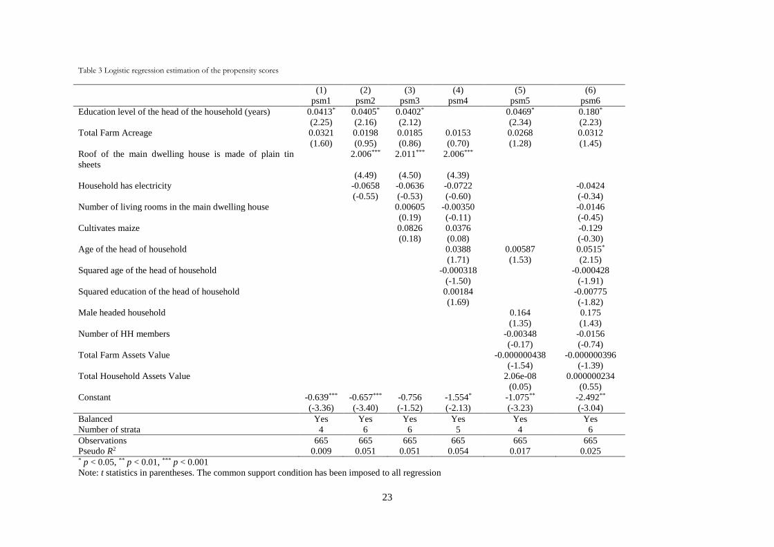
the variance of the estimates. Table 3 presents the results of a logistic (logit model) for different

specifications of the propensity scores. Those specifications inform us on the probability of

participation in the extension program, given a set of covariates The first score (psm1) is a

35 In cases, as the current one, where X is a set of various continuous variables, we would need an

infinitely large set of data in order to match on exact covariates.

22

simple specification that includes only basic regressors. We present 6 different models, using

different specifications in each to address the robustness of the chosen specification. All

specifications respect the balancing condition. Models psm1 and psm5 show overall lower

explanatory power, and both show the unattractive feature of only 4 strata. Figure A.5 in

appendix plots the density function of the different propensity scores specifications. We can

observe there that psm5 produces the best distribution in terms of smoothness, while psm6 has

also a relatively smooth distribution.

Additionally, Table A.1 in appendix presents the comparison of overall significance level and

overall mean standardized36 bias, pre- and post-matching. In theory, after matching, we should

observe a low significance level, an insignificant p-value and a decrease in overall mean

standardized bias. Rosenbaum and Rubin (1985) note that the focus should be on individual

covariate bias exceeding 20% Our most exhaustive models, psm5 and psm6, show little

significant bias37 on individual covariates with 6.8% on the variable “Number of Household

Members” and -10.6% for “Household has electricity” for psm5, while psm6 shows 6.8% bias

for the variable “Number of Household Members”. An examination reveals that psm5

minimizes the overall mean standardized bias by 51% (to 6.4%), and psm6 reduces the bias by

50% (to 5.7%).

36 Following (Rosenbaum & Rubin, 1985), mean standardized bias is the difference in marginal

distributions of the control covariates (X). Formally, the pre-matching mean standardized bias is defined

as 𝑆𝐵𝑏𝑒𝑓𝑜𝑟𝑒 = 100 ×𝑋1 −𝑋0

√0.5×(𝑉1(𝑋)+𝑉0(𝑋))

and the post-matching mean standardized bias is defined as

𝑆𝐵𝑎𝑓𝑡𝑒𝑟 = 100 ×𝑋1𝑀 −𝑋0𝑀

√0.5×(𝑉1𝑀(𝑋)+𝑉0𝑀(𝑋))

, where 𝑋1 and 𝑋0

are the sample means in the treated and control

group and 𝑉1(𝑋) and 𝑉0(𝑋) are the sample variances in the treated and control group. 37 The results of covariate imbalances are not reported exhaustively in the paper.

23

Table 3 Logistic regression estimation of the propensity scores

(1) (2) (3) (4) (5) (6)

psm1 psm2 psm3 psm4 psm5 psm6

Education level of the head of the household (years) 0.0413* 0.0405* 0.0402* 0.0469* 0.180*

(2.25) (2.16) (2.12) (2.34) (2.23)

Total Farm Acreage 0.0321 0.0198 0.0185 0.0153 0.0268 0.0312

(1.60) (0.95) (0.86) (0.70) (1.28) (1.45)

Roof of the main dwelling house is made of plain tin

sheets

2.006*** 2.011*** 2.006***

(4.49) (4.50) (4.39)

Household has electricity -0.0658 -0.0636 -0.0722 -0.0424

(-0.55) (-0.53) (-0.60) (-0.34)

Number of living rooms in the main dwelling house 0.00605 -0.00350 -0.0146

(0.19) (-0.11) (-0.45)

Cultivates maize 0.0826 0.0376 -0.129

(0.18) (0.08) (-0.30)

Age of the head of household 0.0388 0.00587 0.0515*

(1.71) (1.53) (2.15)

Squared age of the head of household -0.000318 -0.000428

(-1.50) (-1.91)

Squared education of the head of household 0.00184 -0.00775

(1.69) (-1.82)

Male headed household 0.164 0.175

(1.35) (1.43)

Number of HH members -0.00348 -0.0156

(-0.17) (-0.74)

Total Farm Assets Value -0.000000438 -0.000000396

(-1.54) (-1.39)

Total Household Assets Value 2.06e-08 0.000000234

(0.05) (0.55)

Constant -0.639*** -0.657*** -0.756 -1.554* -1.075** -2.492**

(-3.36) (-3.40) (-1.52) (-2.13) (-3.23) (-3.04)

Balanced Yes Yes Yes Yes Yes Yes

Number of strata 4 6 6 5 4 6

Observations 665 665 665 665 665 665

Pseudo R2 0.009 0.051 0.051 0.054 0.017 0.025 * p < 0.05, ** p < 0.01, *** p < 0.001

Note: t statistics in parentheses. The common support condition has been imposed to all regression

24

5. Results

We have chosen specific outcomes38 that the NALEP program was targeting, in order to assess

the long-term adoption rate of the program takers, vis-à-vis their control group peers. We

basically see the outcomes separated in 4 main groups: adoption of extension methods, farm

output, revenue, and basic household welfare.

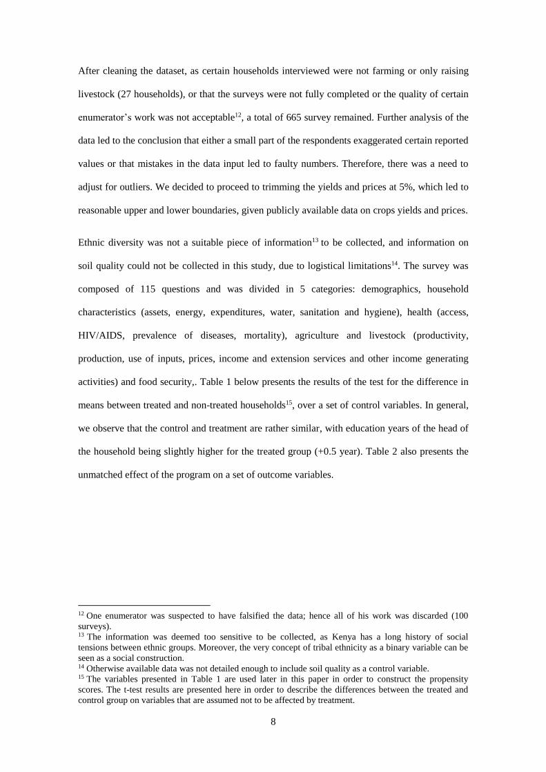
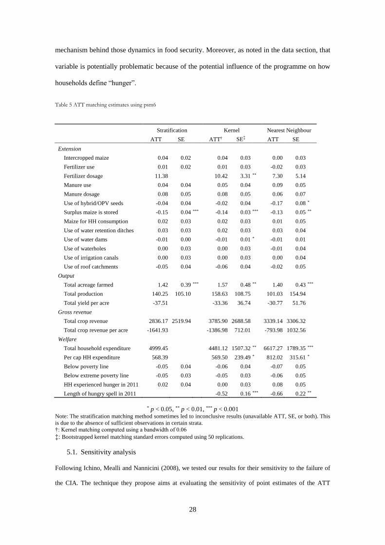
Table 5 below presents the ATT estimates for our set of outcome variables, using the most

exhaustive score specification (psm6). We also present in appendix, under Table A.2, the ATT

estimates using an alternate score specification (psm5), for good measure. Each line corresponds

to a separate estimation, where we used the three different matching methods defined

previously, in order to assess the robustness of our estimation. The common support condition

was also imposed on all estimations. As far as we know, there is no test for overall significance

in a PSM setting, to handle problems related to multiple comparisons. Several estimations use

an aggregate covariate as outcome variable (i.e. revenue, expenditures), while it was not

possible to build a sensitive aggregate function for most technology adoption factors (since they

are often dichotomous). Aggregate covariates serve as an index function, in order to tackle the

issue of spurious relationships.

We see that the overall results are robust across the matching methods, with similar estimates

and standard errors. Comparing the results between the use of psm5 and psm6, we see little

deviation on individual ATT estimates with the stratification and kernel matching method;

significant ATT estimates vary on average39 by 6.2% and 2.2% respectively, while nearest

neighbour matching exhibits more sensitivity towards the score specification, as the estimates

vary by 17.5% between the specifications.

38 We perform 29 estimations, each over a key outcome. This can be seen as a large number of

estimations, compared to the standard economic literature, yet among the research of agricultural

programme evaluation, it is a rather common procedure. Also, it is worth reminding that we analyse

technological packages that are likely to influence a set of outcomes. 39 Taking the average absolute deviation of significant matched ATT estimates between psm5 and psm6.

25

In terms of adoption of extensions methods, the ATT estimates40 show that treated households

use between 7.30 and 11.38 kg/acre of commercial fertilizer more than their control

counterparts, although the significance varies across the methods. Control households use on

average 40.79 kg/acre of commercial fertilizer, meaning that treated households reach on

average the recommended fertilizer dosage (50 kg/acre). This represents an increase in fertilizer

use of 23.78% on average. We did not otherwise find evidence that treated households were

more likely to use other inputs such as high yielding seeds and open pollinated seeds varieties

(OPV), probably because the usage rate of the control group is already very high (89%). On the

topic of technology adoption, there are no sign showing that water harvesting technologies have

been more adopted by the treated households.

In terms of post-harvest handling, we find that the households in the treated group were between

13% and 15% less likely to store the maize surplus. It is not clear what this last finding implies,

as it could on one hand imply good marketing efforts to increase stock turn-over and reduce

inventories, while it can on the other hand mean that treated households do not seem to respond

to storage methods promoted by the program.

In terms of output, there is no sign that the treated households were more productive than the

control households. The key element behind this farming might lay in the fact that Kenya was

affected by the so-called corn lethal necrosis, as explained in introduction. A mitigation strategy

promoted by the Ministry of Agriculture field staff was to rotate crops, more specifically to

avoid planting maize during the 2nd harvest, as to eliminate the breeding ground for the virus.

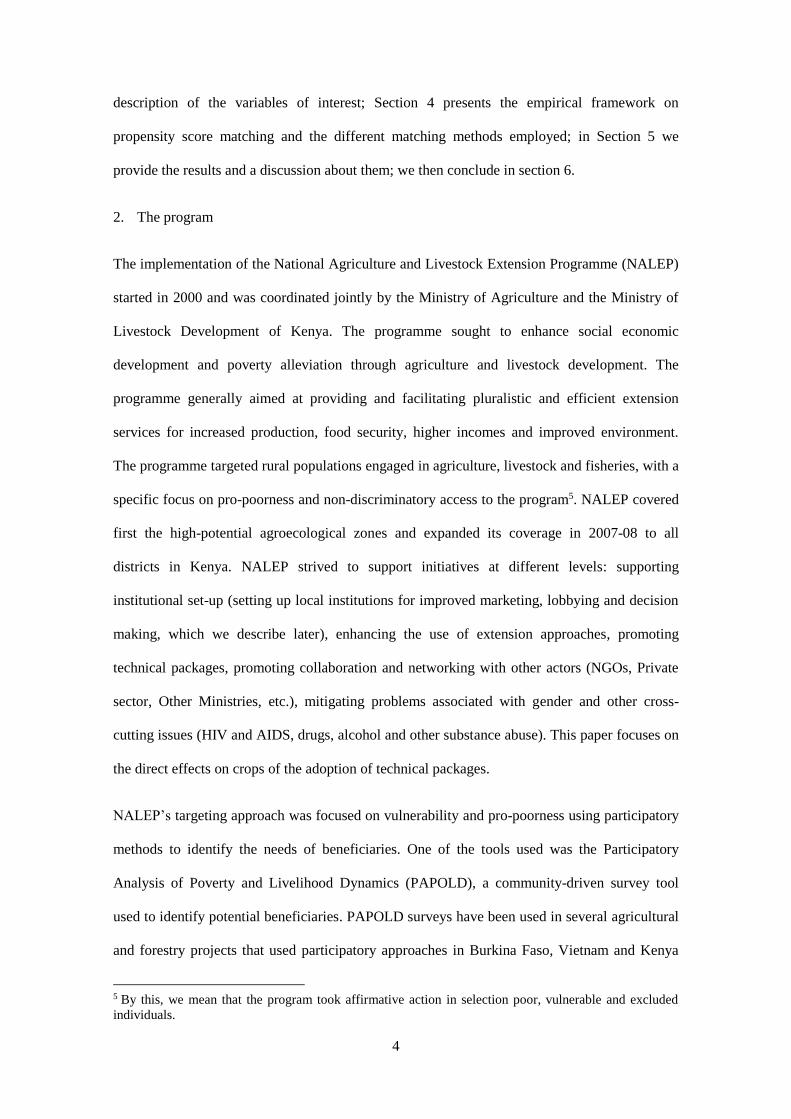
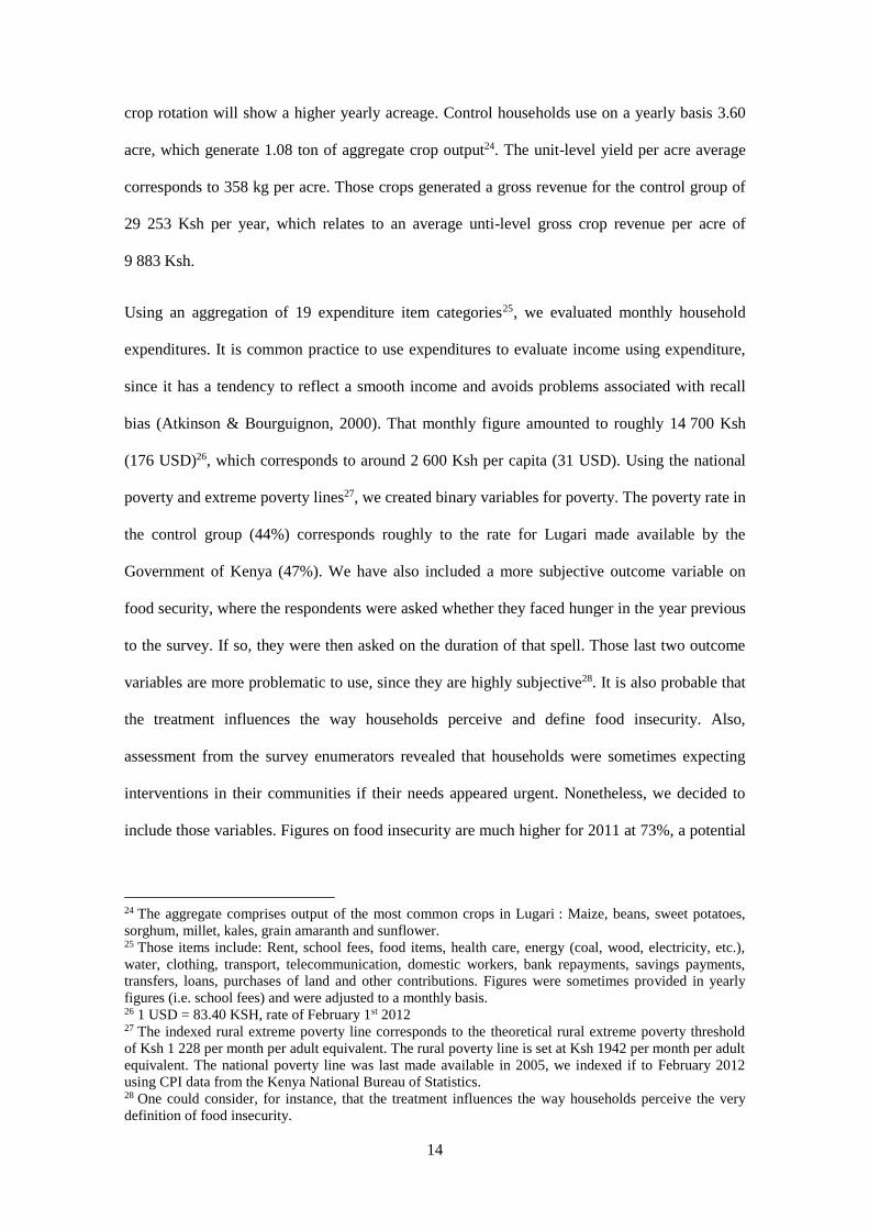
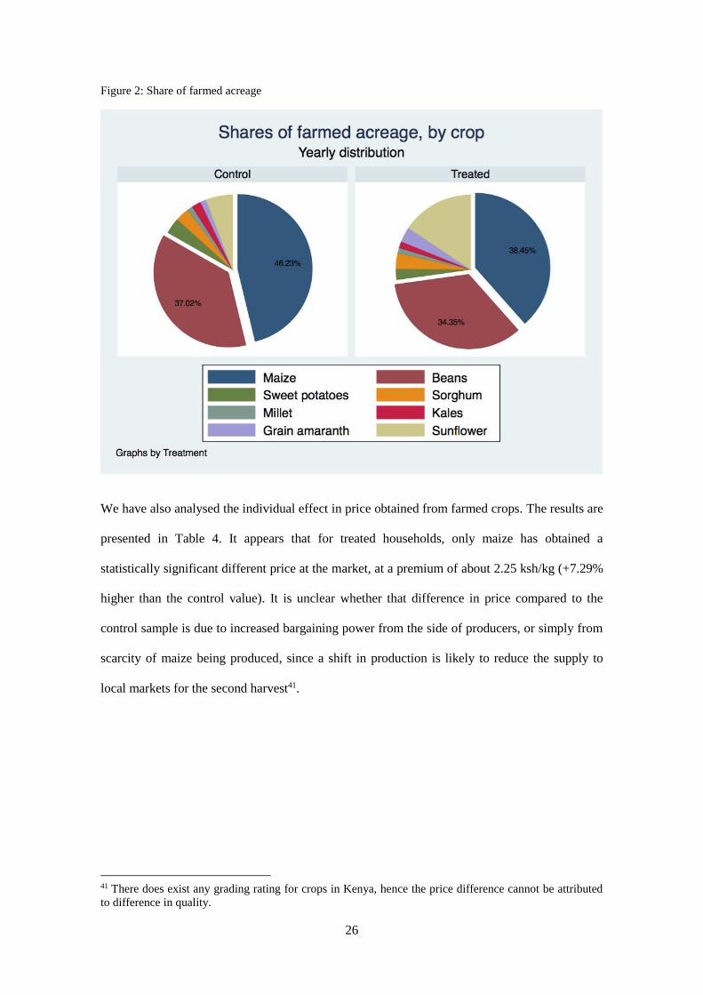
The outcome “total acreage farmed” translates the fact that treated households have farmed a

larger number of acres, by 1.46 acre on average. Figure 2 below shows the composition of farm

crop distribution on farms for the whole 2011 year (for both harvests). Even if we cannot draw

any causal conclusion using such representation, we have evidence that the treated group

seemed to have moved away from the traditional heavy reliance on maize. Instead we observe a

substitution in production towards usually more marginal crops.

40 All the following results are based on psm6.

26

Figure 2: Share of farmed acreage

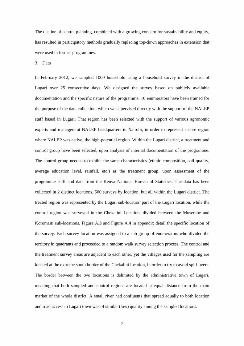
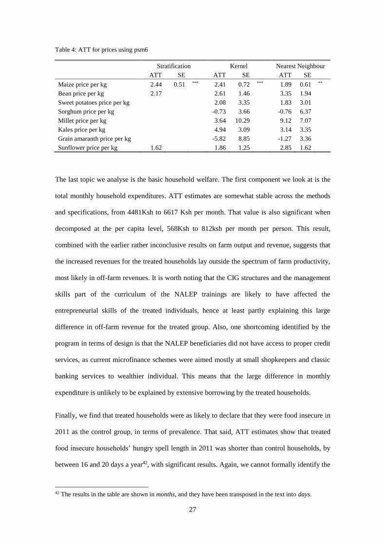
We have also analysed the individual effect in price obtained from farmed crops. The results are

presented in Table 4. It appears that for treated households, only maize has obtained a

statistically significant different price at the market, at a premium of about 2.25 ksh/kg (+7.29%

higher than the control value). It is unclear whether that difference in price compared to the

control sample is due to increased bargaining power from the side of producers, or simply from

scarcity of maize being produced, since a shift in production is likely to reduce the supply to

local markets for the second harvest41.

41 There does exist any grading rating for crops in Kenya, hence the price difference cannot be attributed

to difference in quality.

27

Table 4: ATT for prices using psm6

Stratification Kernel Nearest Neighbour

ATT SE ATT SE ATT SE

Maize price per kg 2.44 0.51 *** 2.41 0.72 *** 1.89 0.61 **

Bean price per kg 2.17

2.61 1.46

3.35 1.94

Sweet potatoes price per kg

2.08 3.35

1.83 3.01

Sorghum price per kg

-0.73 3.66

-0.76 6.37

Millet price per kg

3.64 10.29

9.12 7.07

Kales price per kg

4.94 3.09

3.14 3.35

Grain amaranth price per kg

-5.82 8.85

-1.27 3.36

Sunflower price per kg 1.62

1.86 1.25

2.85 1.62

The last topic we analyse is the basic household welfare. The first component we look at is the

total monthly household expenditures. ATT estimates are somewhat stable across the methods

and specifications, from 4481Ksh to 6617 Ksh per month. That value is also significant when

decomposed at the per capita level, 568Ksh to 812ksh per month per person. This result,

combined with the earlier rather inconclusive results on farm output and revenue, suggests that

the increased revenues for the treated households lay outside the spectrum of farm productivity,

most likely in off-farm revenues. It is worth noting that the CIG structures and the management

skills part of the curriculum of the NALEP trainings are likely to have affected the

entrepreneurial skills of the treated individuals, hence at least partly explaining this large

difference in off-farm revenue for the treated group. Also, one shortcoming identified by the

program in terms of design is that the NALEP beneficiaries did not have access to proper credit

services, as current microfinance schemes were aimed mostly at small shopkeepers and classic

banking services to wealthier individual. This means that the large difference in monthly

expenditure is unlikely to be explained by extensive borrowing by the treated households.

Finally, we find that treated households were as likely to declare that they were food insecure in

2011 as the control group, in terms of prevalence. That said, ATT estimates show that treated

food insecure households’ hungry spell length in 2011 was shorter than control households, by

between 16 and 20 days a year42, with significant results. Again, we cannot formally identify the

42 The results in the table are shown in months, and they have been transposed in the text into days.

28

mechanism behind those dynamics in food security. Moreover, as noted in the data section, that

variable is potentially problematic because of the potential influence of the programme on how

households define “hunger”.

Table 5 ATT matching estimates using psm6

Stratification Kernel Nearest Neighbour

ATT SE ATT† SE‡ ATT SE

Extension

Intercropped maize 0.04 0.02

0.04 0.03

0.00 0.03

Fertilizer use 0.01 0.02

0.01 0.03

-0.02 0.03

Fertilizer dosage 11.38

10.42 3.31 ** 7.30 5.14

Manure use 0.04 0.04

0.05 0.04

0.09 0.05

Manure dosage 0.08 0.05

0.08 0.05

0.06 0.07

Use of hybrid/OPV seeds -0.04 0.04

-0.02 0.04

-0.17 0.08 *

Surplus maize is stored -0.15 0.04 *** -0.14 0.03 *** -0.13 0.05 **

Maize for HH consumption 0.02 0.03

0.02 0.03

0.01 0.05

Use of water retention ditches 0.03 0.03

0.02 0.03

0.03 0.04

Use of water dams -0.01 0.00

-0.01 0.01 * -0.01 0.01

Use of waterholes 0.00 0.03

0.00 0.03

-0.01 0.04

Use of irrigation canals 0.00 0.03

0.00 0.03

0.00 0.04

Use of roof catchments -0.05 0.04

-0.06 0.04

-0.02 0.05

Output

Total acreage farmed 1.42 0.39 *** 1.57 0.48 ** 1.40 0.43 ***

Total production 140.25 105.10

158.63 108.75

101.03 154.94

Total yield per acre -37.51

-33.36 36.74

-30.77 51.76

Gross revenue

Total crop revenue 2836.17 2519.94

3785.90 2688.58

3339.14 3306.32

Total crop revenue per acre -1641.93

-1386.98 712.01

-793.98 1032.56

Welfare

Total household expenditure 4999.45

4481.12 1507.32 ** 6617.27 1789.35 ***

Per cap HH expenditure 568.39

569.50 239.49 * 812.02 315.61 *

Below poverty line -0.05 0.04

-0.06 0.04

-0.07 0.05

Below extreme poverty line -0.05 0.03

-0.05 0.03

-0.06 0.05

HH experienced hunger in 2011 0.02 0.04

0.00 0.03

0.08 0.05

Length of hungry spell in 2011

-0.52 0.16 *** -0.66 0.22 **

* p < 0.05, ** p < 0.01, *** p < 0.001 Note: The stratification matching method sometimes led to inconclusive results (unavailable ATT, SE, or both). This

is due to the absence of sufficient observations in certain strata.

†: Kernel matching computed using a bandwidth of 0.06

‡: Bootstrapped kernel matching standard errors computed using 50 replications.

5.1. Sensitivity analysis

Following Ichino, Mealli and Nannicini (2008), we tested our results for their sensitivity to the failure of

the CIA. The technique they propose aims at evaluating the sensitivity of point estimates of the ATT

29

under various scenarios of deviation of the CIA. The scenarios are based on different values of a

simulated confounder U as a matching parameter, generated using different parameters defining the

distribution of U. Given those parameters, we predict a value of the confounding factor for treated and

control households and then re-estimate the ATT including the confounder U. Following Ichino, Mealli

and Nannicini (Ibid), we characterize a binary confounder by the parameters

𝑃𝑟(𝑈 = 1|𝐷 = 𝑖, 𝑌 = 𝑗, 𝑊) = 𝑃𝑟(𝑈 = 1|𝐷 = 𝑖, 𝑌 = 𝑗) ≡ 𝑝𝑖𝑗

where 𝑖, 𝑗 ∈ {0,1} and W a set of observable covariates. The arbitrary values of 𝑝𝑖𝑗 are based either on

calibrated values or on simulated values based on the distribution of observable binary covariates. Using

those different values, we repeat the estimation 100 times and we average out the ATTs obtained in the

simulation. This in turn leads to a point estimate of the ATT given a deviation of the CIA under specific

parameters. In order to evaluate the size of the effect of U on the relative probability to have a positive

outcome in case of no treatment, the authors propose to evaluate a logit model of 𝑃𝑟(𝑌 = 1|𝐷 =

0, 𝑈, 𝑊). They define it the “outcome effect” and it is characterized as the average estimated odds ratio of

the variable U:

𝑃(𝑌 = 1|𝐷 = 0, 𝑈 = 1, 𝑊)𝑃(𝑌 = 0|𝐷 = 0, 𝑈 = 1, 𝑊)

𝑃(𝑌 = 1|𝐷 = 0, 𝑈 = 0, 𝑊)𝑃(𝑌 = 0|𝐷 = 0, 𝑈 = 0, 𝑊)

= Γ

The authors propose to evaluate the so-called “selection effect” by evaluating the logit model 𝑃𝑟(𝐷 =

1|𝑈, 𝑊) , where the odds ratio of U would measure the effect of the confounding factor on the relative

probability of treatment. It is expressed by:

𝑃(𝐷 = 1|𝑈 = 1, 𝑊)𝑃(𝐷 = 0|𝑈 = 1, 𝑊)

𝑃(𝐷 = 1|𝑈 = 0, 𝑊)𝑃(𝐷 = 0|𝑈 = 0, 𝑊)

= Λ

Table 6.A to 6.C below show the results of sensitivity analyses using the nearest neighbour matching

method for the outcome variables total farmed acreage, stored surplus maize and total crop revenue per

acre respectively. We chose the 2 first outcome variables as they represented key findings, while the third

outcome variable was tested as placebo, since no effect was found on the latter. The first line of each table

shows the baseline ATT and standard error, in order to facilitate the comparison with the ATTs for the

simulated confounders. In all cases, the neutral confounder has practically no effect on Γ and Λ , as well

on the ATT. The confounder based on the distribution of the binary variable “gender of the head of the

30

household” in Table 6.A has a p11 value of 0.87, meaning that 87% of treated households are headed by

male, we impose an identical fraction of households advantaged – say by a skill (the unobservable

confounder we are trying to simulate) – and headed by a male (while that is not necessarily the case) and

are assigned a value U of 1. The same logic applies for all pij values in the confounder like sub-table. In

Table 6.A, we see that in the instance of the simulated confounder based on the ownership of a mobile

phone there is no strong effect on the probability of positive total acreage farmed in the case of no

treatment (Γ ≈ 1), as well as the probability of being treated (Λ ≈ 1). Ichino et al. note that both the

outcome and selection effects need to be strong in order to influence the ATT and standard errors. This

represents a key finding, since the total acreage farmed is attributed to government policies and the

diffusion of information related to those policies, and it does not seem that the access to means of

communication has an effect on the use of government policies. Therefore, the outcome can be attributed

to the NALEP treatment. The ATT also does not differ from the baseline scenario under that confounding

factor. The confounder based on the binary variable “bicycle ownership” generates higher values for Γ

and Λ, yet the ATT also remains constant with respect to the baseline scenario. Overall, we observe

strong robustness in the ATT point estimates, as they do not vary across the various simulated

confounder. The same conclusions apply to the simulated confounders included in matching methods

with the outcome variable “surplus maize is stored” and the placebo test on the variable “total crop

revenue per acre”, whereas the simulated deviation of the CIA does not influence the point estimates for

ATT.

31

Table 6.A Sensitivity analysis on the variable "total acreage farmed"

Fraction U=1 by

treatment/outcome

Outcome

effect

Selection

Effect ATT SE

p11 p10 p01 p00 Γ Λ

No confounder 0.00 0.00 0.00 0.00 - - 1.40 0.43

Neutral confounder 0.50 0.50 0.50 0.50 1.02 1.03 1.40 0.43

Confounder like:

Head of HH Gender 0.87 0.75 0.76 0.74 1.17 1.37 1.40 0.43

Owns mobile phone 0.86 0.88 0.87 0.88 1.05 0.98 1.40 0.43

Owns bicycle 0.61 0.48 0.49 0.38 1.73 1.68 1.40 0.43

Table 6.B Sensitivity analysis on the variable "Surplus maize stored"

Fraction U=1 by

treatment/outcome

Outcome

effect

Selection

Effect ATT SE

p11 p10 p01 p00 Γ Λ

No confounder 0.00 0.00 0.00 0.00 - - -0.13 0.05

Neutral confounder 0.50 0.50 0.50 0.50 1.00 0.99 -0.13 0.05

Confounder like:

Head of HH Gender 0.80 0.81 0.74 0.73 1.05 1.55 -0.13 0.05

Owns mobile phone 0.92 0.79 0.89 0.81 2.13 1.05 -0.13 0.05

Owns bicycle 0.50 0.59 0.38 0.40 1.00 1.89 -0.13 0.05

Table 6.C Sensitivity analysis on the variable "total revenue per acre"

Fraction U=1 by

treatment/outcome

Outcome

effect

Selection

Effect ATT SE

p11 p10 p01 p00 Γ Λ

No confounder 0.00 0.00 0.00 0.00 - - -793.98 1032.56

Neutral confounder 0.50 0.50 0.50 0.50 1.02 1.04 -793.98 1032.56

Confounder like:

Head of HH Gender 0.84 0.78 0.76 0.73 1.24 1.39 -793.98 1032.56

Owns mobile phone 0.90 0.86 0.94 0.82 3.97 0.98 -793.98 1032.56

Owns bicycle 0.47 0.57 0.49 0.33 2.02 1.64 -793.98 1032.56

6. Conclusion

This paper was taking on a complex challenge; to evaluate the long-run effect of a government

run extension program on households. Kenya, as many other sub-Saharan countries, has the

potential to uplift millions of households through increased farm productivity and marketing.

This paper emphasized the crucial methodological aspects required for this type of ex-post

analysis, which is a setting that is less resource intensive than randomized experiments.

32

According to the PSM estimation performed in this paper, there are clear signs that the program

has had impacts on the treated households. The increased quantity of fertilizer applied,

corresponding to the recommended dosage, is one of the positive outcome of the program. The

response of treated households in terms of pest mitigation and crop rotation is also crucial and

an important finding. While this is the case, the scope of those impacts are clearly not

corresponding to the general objectives the program had set. We could not find evidence of

improve productivity or improve irrigation, for instance. Overall, the program was aiming at

uplifting agriculture in terms of productivity and to fight poverty. From our perspective,

structural obstacles – such as land rights, access to credit, plot sizes, integrated value chains and

specialization of farmers – restricted what the program could achieve in practice. We believe

that the program was conscious of those constrains, as many of the aforementioned constrains

are addressed by the program that followed NALEP, the Agriculture Sector Development

Support Program (ASDSP). Nonetheless, the results show that the treated households spend

more every month than the control households, while production and productivity is unchanged,

suggesting that off-farm incomes are greater for the NALEP beneficiaries.

The question is then: Why didn’t the program lead to better results? There is much room for

speculation, but certain answers can be sketched. One explanation would be that behavioural

economists point to the works of Dupas (2009) and Ashraf, Berry, & Shapiro (2007) that

suggest that the price of government provided services might affect the way beneficiaries value

the services, and make use of them. As NALEP provided the service for free, as opposed to the

recent Payment for Ecological Services (PES) approach to extension in Uganda, it is possible

that the NALEP beneficiaries did not engage with the treatment to a sufficient extent. Another

explanation of the limited impact of NALEP is the very nature of the beneficiaries. For instance,

the Government of Kenya has laid down plans to modernize the country by 2030 and has set

goals of increased food production, as well as improving the country’s food security status. The

“low hanging fruit solution” for this master plan would for instance involve working closely

with large-scale farmers. NALEP targeted the very opposite side of the spectrum of agriculture

33

workers: the poor, small landholder and vulnerable. With such a selection of beneficiaries, it is

arguably understandable that the returns to the program are low, since the beneficiaries are

generally less endowed. Another explanation, more classical in the context of publicly provided

services, is the limited resources of the program. As stated earlier, the program was supposed to

spend 3 years in a focal area, but in practice the involvement was only for one year. This

reduces drastically the potential for learning agricultural techniques that require timing and

happen only once a year (i.e. water harvesting, top-dressing). Hence, it is possible that the

knowledge retention on timely, but crucial, activities has been limited due to limited resources.

In terms of bias of our results, it is also possible that unobservables played a role overall, even

after testing for sensitivity to deviation of the CIA, as we could not match households on soil

quality. Our setting is also prone to problems related to aggregate shocks at the sub-location

level, which is an issue that is yet little understood.

The impact of the adoption of technological packages has not received a lot of attention from

researchers within the field of economics, and it deserves to change. Further applied research

should include better information on the incidence of treatment and the extent of the knowledge

that remains overtime. Godtland et al. (2004) investigated the effect of farmers field schools

(FFS) on potato farmers in Peru, and more of such research should be conducted. Also, this

paper is the result of a cooperation between the programme itself and academics, which has

yielded positive externalities for the programme in developing new evaluation techniques for

their programming purposes.

34

BIBLIOGRAPHY

Abadie, A., & Imbens, G. W. (2006). Large Sample Properties of Matching Estimators for

Average Treatment Effects. Econometrica , 235-267.

Abadie, A., & Imbens, G. W. (2008). On the failure of the bootstrap for matching estimators.

Econometrica , 1537-1557.

Anderson, J. R., & Feder, G. (2004). Agricultural Extension: Good intentions and hard realities.

The World Bank Research Observer , 41-60.

Angrist, J. D., & Pischke, J.-S. (2008). Mostly harmless econometrics: An empiricist's

companion. Princeton University Press.

Ashraf, N., Berry, J., & Shapiro, J. M. (2007). Can higher prices stimulate product use?

Evidence from a field experiment in Zambia. National Bureau of Economic Research (No.

w13247).

Atkinson, A., & Bourguignon, F. (2000). Handbook of Income Distribution.

Augurzky, B., & Schmidt, C. M. (2001). The Propensity Score: A means to An End. IZA

Discussion paper series, No. 271 .

Bassi, L. J. (1984). Estimating the Effect of Training Programs with Non-Random Selection.

The Review of Economics and Statistics , 36-43.

Becerril, J., & Abdulai, A. (2010). The Impact of Improved Maize Varieties on Poverty in

Mexico: A propensity score approach. World Development , 38 (7), 1024-1035.

Becker, S. O., & Ichino, A. (2002). Estimation of average treatment effects based on propensity

scores. The stata journal , 2 (4), 358-377.

Bindlish, V., & Evenson, R. E. (1997). The impact of T&V extension in Africa: The experience

of Kenya and Burkina Faso. The World Bank Research Observer , 183-201.

35

Birkhaeuser, D., & Evenson, R. E. (1991). The Economic Impact of Agricultural Extension: A

Review. Economic Development and Cultural Change , 607-650.

Bryson, A., Dorsett, R., & Purdon, S. (2002). The use of propensity score matching in the

evaluation of active labour market policies. Working Paper, Department for Work and

Pensions, UK .

Caliendo, M., & Kopeinig, S. (2005). Some practical guidance for the implementing of

propensity score matching. IZA Discussion Papers No. 1588 .

Chavas, J.-P., & Cox, T. L. (1992). A nonparametric analysis of the influence of research on

agricultural productivity. American journal of agricultural economics , 583.

Cochrane, W. G., & Rubin, D. B. (1973). Controlling Bias in Observational Studies: A Review.

Sankhyā: The Indian Journal of Statistics , 417-446.

Cochrane, W., & Chambers, P. S. (1965). The Planning of Observational Studies of Human

Populations. Journal of the Royal Statistical Society , 234-266.

Cuellar, M., Hedlund, H., Mbai, J., & Mwangi, J. (2006). The National Agriculture and

Livestock Extension Programme Phase I: Impact Assesment. Stockholm: Swedish International

Development Agency, Department for Africa.

de Janvry, A., & Sadoulet, E. (2010). Agricultural Growth and Poverty Reduction: Additional

Evidence. World Bank Research Observer , 25 (1), 1-20.

Dehejia, R. H., & Wahba, S. (2002). Propensity Score-Matching Methods for Nonexperimental

Causal Studies. The Review of Economics and Statistics , 151-161.

Dercon, S. e. (2009). The impact of agricultural extension and roads on poverty and

consumption growth in fifteen Ethiopian villages. American Journal of Agricultural Economics

, 91 (4), 1007-1021.

36

DiNardo, J., & Tobias, J. L. (2001). Nonparametric density and regression estimation. The

Journal of Economic Perspectives , 11-28.

Dupas, P. (2009). What matters (and what does not) in households' decision to invest in malaria

prevention?. The American Economic Review , 99 (2), 224-230.

Famine Early Warning Systems Network. (2013). Africa Data Portal. Reston, VA: US

Geological Survey.

Foster, A. D., & Rosenzweig, M. R. (1996). Technical change and human-capital returns and

investments: evidence from the green revolution. The American economic review , 931-953.

Friedlander, D., Greenberg, D. H., & Robins, P. K. (1997). Evaluating Government Training

Programs for the Economically Disadvantaged. Journal of Economic Literature , 1809-1855.

Githaiga, R. W. (2007). Economic and Social Impacts of the Common Interest Group Approach

to Public Agricultural Extension in Kenya. Journal of Developments in Sustainable Agriculture

, 159-166.

Godtland, E. M., Sadoulet, E., de Janvry, A., Murgai, R., & Ortiz, O. (2004). The Impact of

Farmer-Field-Schools on Knowledge and Productivity: A Study of Potato Farmers in the

Peruvian Andes. Economic Development and Cultural Change , 63-92.

Hahn, J. (1998). On the Role of the Propensity Score in Efficient Semiparametric Estimation of

Average Treatment Effects. Econometrica , 315-331.

Heckman, J. J., Ichimura, H., & Todd, P. E. (1997). Matching as an Econometric Evaluation

Estimator: Evidence from Evaluating a Job Training Programme. Review of Economic Studies ,

605-654.

Heckman, J. J., Lalonde, R. J., & Smith, J. A. (1999). The economics and econometrics of

active labor market programs. In Handbook of Labor Economics (pp. 1865-2097).

37

Heckman, J., & Navarro-Lozano, S. (2004). Using Matching, Instrumental Variables, and

Control Functions to Estimate Economic Choice Models. The Review of Economics and

Statistics , 30-57.

Hoang, M. H., & Nguyen, H. Q. (2011). Tools for use in Integrated Natural Resources

Management (INRM) and Payment for Environmental Services in Vietnam. Lecture notes , 1 ,

89. Vietnam: World Agroforestry Center (ICRAF).

Ichino, A., Mealli, F., & Nannicini, T. (2008). From temporary help jobs to permanent

employment: what can we learn from matching estimators and their sensitivity? . Journal of

Applied Econometrics , 23 (3), 305-327.

Imbens, G. W. (2004). Nonparametric Estimation of Average Treatment Effects under

Exogeneity: A Review. The Review of Economics and Statistics , 4-29.

Jalan, J., & Ravallion, M. (2003). Estimating the benefit incidence of an antipoverty program by

propensity-score matching. Journal of Business & Economic Statistics , 21 (1), 19-30.

Jones, P. G., & Thornton, P. K. (2003). The potential impacts of climate change on maize

production in Africa and Latin America in 2055. Global Environmental Change , 13 (1), 51-59.

Kenya Meteorological Department. (2013, Feb 11). Drought in Africa. Retrieved Feb 28, 2013

from http://www.meteo.go.ke/imtr/Understanding%20Droughts.pdf

Khan, Z. R., Pickett, J. A., van den Berg, J., Wadhams, L. J., & Woodcock, C. M. (2000).

Exploiting chemical ecology and species diversity: stem borer and striga control for maize and

sorghum in Africa. Pest management science , 957-962.

Lechner, M. (2002). Program heterogeneity and propensity score matching: An application to

the evaluation of active labor market policies. Review of Economics and Statistics , 84 (2), 205-

220.

38

Mendola, M. (2007). Agricultural technology adoption and poverty reduction: A propensity-

score matching analysis for rural Bangladesh. Food Policy , 372-393.

Ochieng, J., Wangai, A., Miyogo, S., Karanja, T., Oduor, H., Kimani, E., et al. (2012). Status of

Maize Lethal Necrosis Disease and General Maize Performance. Ministry of Agriculture of

Kenya.

Pinstrup-Andersen, P. (1985). Food prices and the poor in developing countries. European

Review of Agricultural Economics , 69-85.

Ravallion, M., & Datt, G. (1998). Farm Productivity and Rural Poverty in India. Journal of

Development Studies , 62-85.

Rosenbaum, P. R., & Rubin, D. B. (1985). Constructing a Control Group Using Multivariate

Matched Sampling Methods That Incorporate the Propensity Score. The American Statistician ,

33-38.

Rosenbaum, P. R., & Rubin, D. B. (1984). Reducing bias in observational studies using

subclassification on the propensity score. Journal of the American Statistical Association , 79

(387), 516-524.

Rosenbaum, P. R., & Rubin, D. B. (1983). The Central Role of the Propensity Score in

Observational Studies for Causal Effects. Biometrika , 41-55.

Rubin, D. B. (1973). Matching to Remove Bias in Observational Studies. Biometrics , 159-183.

Rubin, D. B. (1979). Using Multivariate Matched Sampling and Regression Adjustment to

Control Bias in Observational Studies. Journal of the American Statistical Association , 318-

328.

Smith, J. A., & Todd, P. A. (2005). Does matching overcome LaLonde's critique of

nonexperimental estimators? Journal of Econometrics , 305-353.

39

Swinkels, R., & Franzel, S. (1997). Adoption potential of hedgerow intercropping in maize-

based cropping systems in the highlands of western Kenya. Experimental Agriculture , 211-223.

Thirtle, C., Lin, L., & Piesse, J. (2003). The impact of research-led agricultural productivity

growth on poverty reduction in Africa, Asia and Latin America. World Development , 31 (12),

1959-1975.

World Bank. (2013). World Development Indicators: Kenya. Washington: The World Bank.

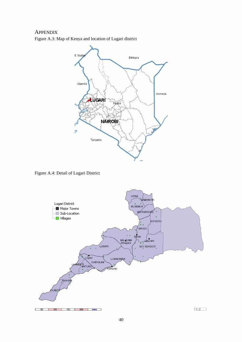
40

APPENDIX Figure A.3: Map of Kenya and location of Lugari district

Figure A.4: Detail of Lugari District

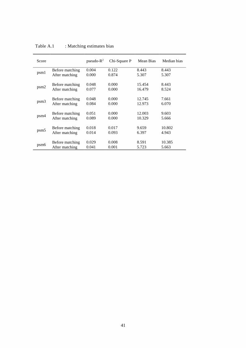
41

Table A.1 : Matching estimates bias

Score

pseudo-R2 Chi-Square P Mean Bias Median bias

psm1 Before matching 0.004 0.122 8.443 8.443

After matching 0.000 0.874 5.307 5.307

psm2 Before matching 0.048 0.000 15.454 8.443

After matching 0.077 0.000 16.479 8.524

psm3 Before matching 0.048 0.000 12.745 7.661

After matching 0.084 0.000 12.973 6.070

psm4 Before matching 0.051 0.000 12.003 9.603

After matching 0.089 0.000 10.329 5.666

psm5 Before matching 0.018 0.017 9.659 10.802

After matching 0.014 0.093 6.397 4.943

psm6 Before matching 0.029 0.008 8.591 10.385

After matching 0.041 0.001 5.723 5.663

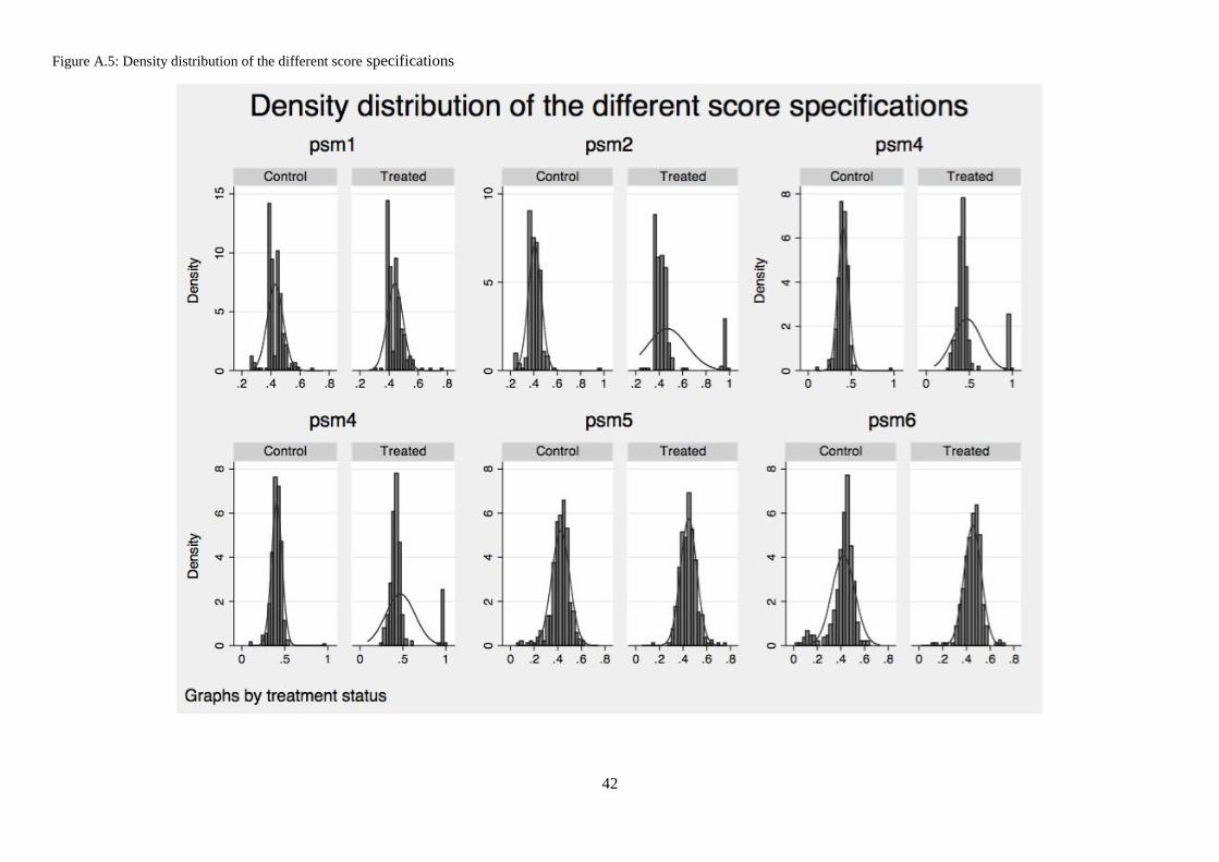
42

Figure A.5: Density distribution of the different score specifications

43

Table A.2 : ATT estimates for various outcomes variables, using psm5

Stratification Kernel Nearest Neighbour

ATT SE ATT SE ATT SE

Extension

Intercropped maize 0.04 0.02 0.04 0.02 0.07 0.04 *

Fertilizer use 0.01 0.02 0.01 0.02 0.01 0.03

Fertilizer dosage 10.08 10.08 3.60 ** 12.87 4.27 **

Manure use 0.06 0.04 0.06 0.04 0.03 0.05

Manure dosage 0.09 0.05 0.07 0.05 0.12 0.07

Use of hybrid/OPV seeds -0.04 0.04 -0.04 0.04 -0.07 0.07

Surplus maize is stored -0.13 0.04 *** -0.13 0.04 ** -0.17 0.05 ***

Maize for HH consumption 0.01 0.03 0.02 0.03 -0.06 0.05

Use of water retention ditches 0.01 0.03 0.02 0.03 -0.02 0.04

Use of water dams -0.01 0.00 * -0.01 0.01 -0.01 0.01

Use of waterholes 0.00 0.03 0.00 0.02 -0.03 0.03

Use of irrigation canals 0.00 0.03 0.00 0.03 -0.06 0.04

Use of roof catchments -0.05 0.04 -0.05 0.04 0.00 0.05

Output

Total acreage farmed 1.14 0.41 ** 1.52 0.40 *** 1.71 0.39 ***

Total production 306.27 209.67 299.70 222.78 129.21 230.72

Total yield per acre -7.55 42.67 -16.76 48.87 -73.02 52.24

Gross revenue

Total crop revenue 3369.34 2575.58 3584.02 2446.62 1085.75 3254.39

Total crop revenue per acre

-1124.41 770.05 -1301.66 843.21 -

2364.83

998.95 *

Welfare

Total household expenditure 4131.56 1996.16 * 3406.22 1949.83

Per cap HH expenditure 515.27 283.87 486.79 349.73

Below poverty line -0.05 0.04 -0.06 0.03 -0.02 0.05

Below extreme poverty line -0.05 0.03 -0.05 0.03 -0.02 0.05

HH experienced hunger in 2011 0.02 0.04 0.00 0.03 0.02 0.05

Length of hungry spell in 2011 -0.53 0.12 *** -0.53 0.15 *** -0.61 0.20 **

HH experienced hunger in 2010 0.06 0.02 *** 0.06 0.02 *** 0.06 0.02 **

Length of hungry spell in 2010 1.16 1.48 0.90 0.54

* p < 0.05, ** p < 0.01, *** p < 0.001 Note: The stratification matching method sometimes led to inconclusive results (unavailable ATT, SE, or both). This

is due to the absence of sufficient observations in certain strata.

†: Kernel matching computed using a bandwidth of 0.06

‡: Bootstrapped kernel matching standard errors computed using 50 replications.