WP/06/37

The Impact of Foreign Interest Rates on the Economy: The Role of the

Exchange Rate Regime

Julian di Giovanni and

Jay C. Shambaugh

© 2006 International Monetary Fund WP/06/37

IMF Working Paper

Middle East and Central Asia Department

The Impact of Foreign Interest Rates on the Economy: The Role of the Exchange Rate Regime

Prepared by Julian di Giovanni and Jay C. Shambaugh1

Authorized for distribution by Edward Gardner

February 2006

Abstract

This Working Paper should not be reported as representing the views of the IMF. The views expressed in this Working Paper are those of the author(s) and do not necessarily represent those of the IMF or IMF policy. Working Papers describe research in progress by the author(s) and are published to elicit comments and to further debate.

This paper explores the connection between interest rates in major industrial countries and annual real output growth in other countries. The results show that high large-country interestrates have a contractionary effect on annual real GDP growth in the domestic economy, but that this effect is centered on countries with fixed exchange rates. The paper then examines the potential channels through which large-country interest rates affect small economies. Thedirect monetary policy channel is the most likely channel when compared with other possibilities, such as a general capital market effect or a trade effect. JEL Classification Numbers: F3; F4 Keywords: Exchange rate regime; international transmission; interest rates Author(s) E-Mail Address: JdiGiovanni@imf.org, Jay.C.Shambaugh@Dartmouth.edu

1 Jay C. Shambaugh is Professor of Economics at Dartmouth College. We thank Andrew Bernard, Pierre-Olivier Gourinchas, Gian Maria Milesi-Ferretti, Romain Rancière, Alessandro Rebucci, Tiago Ribeiro, Andrew Rose, and participants at several seminars for comments. We also thank Justin McCrary, Maury Obstfeld, David Romer, and Till von Wachter for very useful conversations. Part of this research was conducted while Jay Shambaugh was a Visiting Scholar at the IMF and at the Institute for International Integration Studies at Trinity College Dublin.

- 2 -

Contents PageI. Introduction.................................................................................................. 3

II. Conceptual Framework ................................................................................... 7

III. Empirical Framework ..................................................................................... 8A. Random Coefficients Model ................................................................... 11

IV. Data and Results............................................................................................ 12A. Data .................................................................................................. 12B. Panel Estimation .................................................................................. 12C. Random Coefficients Estimation.............................................................. 17D. Channels ............................................................................................ 19

V. Conclusion ................................................................................................... 23

AppendixesI. Data............................................................................................................ 25II. Estimation of RCM Model............................................................................... 28

Tables1. Effects of Base Interest Rate on Real Output Growth:

Baseline Least Square Estimates ...................................................................... 292. Effects of Base Interest Rate on Real Output Growth: Additional Controls ............... 303. Effects of Base Interest Rate on Real Output Growth: Subsamples of Data ................ 314. Considering Non-Base Interest Rates ............................................................... 325. Explanation of Base Interest Rate Impact on Real Output Growth: Random

Coefficients Model ....................................................................................... 336. Impact of Change in Base Interest Rates and Spread on

Change in Domestic Interest Rates ................................................................... 347. Other Channels and Base Interest Rate .............................................................. 35

Appendix TablesA1. Sample Summary Statistics ............................................................................ 35A2. Effects of Base and U.S. Interest Rates on Real Investment Growth ........................ 36A3. Different Cuts of Data to Exclude Outlier Periods and Observations ........................ 37A4. Examination of Different Exchange Rate Regimes’ Classifications ......................... 38A5. Examination on Reinhart and Rogoff’s Five-Way Breakdown of Exchange Rate

Regimes ..................................................................................................... 39

Figure1. Impact of Exchange Rate Regime on Estimated Base Interest Rate Coefficients ......... 40

References ........................................................................................................ 41

- 3 -

I. INTRODUCTION

Discussions of globalization often assert that the fortunes of small countries are driven bylarger countries’ economies. This notion contends that small countries are highly susceptibleto conditions in large countries and that their economies often experience volatility forreasons independent of domestic policies. One assumption underlying this idea is that foreigninterest rates have a strong impact on conditions in smaller countries. At the same time, theopen economy “trilemma” and empirical tests of it suggest that only countries with peggedexchange rate regimes give up their domestic monetary autonomy.2 The monetary policyconstraints suggested by the trilemma imply that the channel through which foreign interestrates affect smaller economies determines whether large country interest rates have the sameeffect on pegs and floats.3 Pegs are expected to be more affected if the channel is monetary;but if the main channel is simply a general capital market effect, the exchange rate regimemay be irrelevant.

This paper answers two questions. First, what is the effect of interest rates in base countrieson other countries’ annual real GDP growth? Second, how does this effect vary byinstitutional arrangement (primarily the exchange rate regime) and other countrycharacteristics? Answering the second question helps to disentangle the channels throughwhich large-country interest rates affect other economies.

We find that annual real output growth in small countries is negatively associated with interestrates in base countries,4 but that this effect holds only for countries with fixed exchange rates.This finding is robust across a wide set of specifications, and suggests that the primary impactof foreign interest rates is through the monetary policy channel and not as strongly through ageneral capital market effect. Additional work exploring potential channels supports theseimplications. This result suggests that there are real costs to the loss of monetary autonomythat comes with pegging and provides further support for the hypothesis that monetary policyand interest rates can have substantial effects on the real economy.

2 The trilemma is the conjecture that at any one time a country can pursue only two of thethree following options: a fixed exchange rate, open capital markets, and monetary autonomy;this is the case because a fixed exchange rate and open capital markets will imply by interestparity that a country has lost its monetary autonomy. See Obstfeld, Shambaugh, and Taylor(2005) for discussion of the trilemma and empirical tests.

3 A “peg” will henceforth refer to a country whose exchange rate stays within a prescribedrange, while “float” and “nonpeg” will be used interchangeably to refer to any country that isnot pegged.

4 The “base country” is the country to which a country pegs or the country to which it wouldpeg if it were pegged. The discussion in Section IV regarding the definition of fixed exchangerates will elaborate.

- 4 -

Specifically, base-country interest rates that are 5 percentage points (500 basis points) higherlead to a 1 percentage point decline in annual GDP growth in pegged countries as opposed tono change in countries with floats. This result is robust to a variety of controls for year,country, income, and capital controls, and holds when we run the regressions on samplesdivided by region or income level. In addition, the results are consistent with a wide variety ofspecifications that add in base-country annual GDP growth and other covariates. Further,when one is considering a variety of country characteristics that could drive the relationshipbetween domestic output movements and the base interest rate, the exchange rate regime isconsistently an important factor and few other factors have such a robust effect.

By including a broad panel of countries that have different base countries, this study has anadvantage over previous research, in that we are able to use time controls and focus on thespecific effect of the base interest rate. Thus, our panel allows us to strip out both individualcountry effects and worldwide movements in growth rates providing a better identification ofthe effect we study. Furthermore, we find that countries pegged to currencies other than theU.S. dollar do not respond to dollar interest rates any more than floats do. This suggests thatpegged economies are not simply more exposed to world markets, but in fact are moreexposed to the interest rate of the countries to which they peg. Results such as these havenever been pursued before, given small samples or a focus on one world rate of interest.

Finally, when examining channels, we find that the base rate does not appear to have an effecton variables such as exports to the base country. Furthermore, a variety of specifications ofcapital flows regressed on the base interest rate do not seem to show strong results for eitherpegs or floats. On the other hand, base interest rates do have an impact on domestic interestrates and the impact is much stronger for pegs. This finding, along with the differences seenacross exchange rate regimes, suggests that the direct monetary policy channel may be theprimary channel through which interest rates affect other countries. The finding that baseinterest rates affect pegs more than floats is consistent with recent evidence that while manycountries may show “fear of floating,” countries that actually do float show far less connectionto base interest rates than countries that peg (Shambaugh, 2004; and Obstfeld, Shambaugh,and Taylor, 2004, 2005).

These results are important both for understanding how and why monetary policy istransmitted around the world and how the exchange rate regime allows a country to insulateitself from conditions in large countries. Moreover, these results do not suggest that a peggedregime is either a good or bad idea, but instead add to the calculus of costs and benefits (inthis case costs) an economy will face when it fixes its exchange rate.

This paper sits at the nexus of two literatures: (i) the impact of monetary policy on theeconomy, and (ii) the impact of large countries on smaller countries’ business cycles. There isan extensive literature on the impact of monetary policy on the economy.5 In

5 This literature is too broad to distill here, see Christiano, Eichenbaum, and Evans (1999)for discussion.

- 5 -

general, the literature finds that increasing interest rates has a negative effect on the realeconomy.

Di Giovanni, McCrary, and von Wachter’s (2005) contribution is the most relevant for thepresent paper. The authors argue that the EMS/ERM era provides a “quasi-experimental”setting, whereby European countries were inclined to follow German monetary policy due tovarious institutional constraints, in order to test for the causal impact of domestic monetarypolicy in these other countries. As such, di Giovanni, McCrary, and von Wachter instrumentdomestic interest rates with the German one in order to test for the impact of domesticmonetary policy, and find a strong effect. Furthermore, the paper quantifies the size of the biasbetween the ordinary least squares and instrumental variables estimates of the impact ofmonetary policy, provides a rigorous treatment that relates the size of the bias to underlyingshocks in the system, and derives a dynamic interpretation of their results.6

The literature on how large countries affect developing countries’ economies is also relevant.Dornbusch (1985) considers the role of large-country business cycles in determiningcommodity prices and, subsequently, other outcomes for developing countries. Calvo,Leiderman, and Reinhart (1993 and 1996) focus on the interest rates of large countries andargue that owing to capital market links, low interest rates in large countries tend to sendinvestors looking for high-yield investments in other countries. This process generates capitalinflows for developing countries, which could then reverse when large-country interest ratesincrease.

There also have been several attempts to untangle the impact of large-country interest rates ondomestic annual GDP growth. Reinhart and Reinhart (2001) consider a variety of North-Southlinks when examining Group of Three (G-3) interest rate and exchange rate volatility. Theyfind that capital tends to flow to emerging markets when the U.S. eases its monetary policy,but they do not see a connection between such changes in the Fed Funds rate and growth inemerging market economies. However, they do find an effect of the U.S. real interest rate ongrowth in some regions. Frankel and Roubini (2001) also find a negative effect of G-7 realinterest rates on developing countries’ output. Since these papers consider many aspects ofNorth-South relations, they do not have space to consider in detail how large-country interestrates and the domestic economy are connected. In particular, they do not consider how theserelationships vary across institutional details (e.g., exchange rate or capital controls regimes),test what the channels may be, or conduct detailed robustness checks, nor do they have thesample breadth to exploit multiple base interest rates as we are able to do.

6 See di Giovanni, McCrary, and von Wachter (2005) and Section III of the present paper formore details. Section III also provides an explanation of why the present paper does notundertake an IV strategy.

- 6 -

In addition to these two studies, there have been a number of papers that use vectorautoregressions (VARs) to explore the transmission of international business cycles.7 Anotable contribution is Kim (2001), which finds that U.S. interest rates have an impact onoutput in the other six G-7 countries. This paper is one of the few to examine the potentialchannels through which the interest rate has an effect. It finds virtually no trade impact andthat the impact on output comes from a reduction in the world interest rate.8

What has been largely absent from the literature, though, is the fact that the exchange rateregime should play a major role in how foreign interest rates are transmitted.9 The openeconomy trilemma suggests that countries with open capital markets and pegged exchangerates sacrifice monetary autonomy and must follow the base country. Work by Shambaugh(2004) and Obstfeld, Shambaugh, and Taylor (2004 and 2005) confirm these predictionsempirically. Thus, countries should not react to changes in large-country interest ratesuniformly. Countries with fixed exchange rates should be the ones most directly affected. Inaddition, pegged countries should not react to simply any large country interest rate shock, butparticularly to the interest rate of the country to which their currencies are pegged.10

In this paper we focus on these insights and try to uncover the impact of large-country interestrates on other countries while paying particular attention to the way the exchange rate regimemay affect the transmission. The paper makes a number of new contributions to the literature.First, it takes the institutional differences across countries seriously. The study focuses on theexchange rate regime and capital control regimes of countries in order to examine theheterogeneous responses to base-country interest rates. Second, a broad data set is used whichincludes almost all countries and relies on differences across countries in the base interest rateto allow for an examination of year controls and to test whether countries respond to largecountry rates in general or only to the base country. This additional power increases

7 See, for example, Canova (2005); Mackowiak (2003); and Miniane and Rogers (2003).

8 All countries studied float their currencies against the U.S. dollar, so there is implicitly nodiscussion of exchange rate regime in the analysis.

9 Broda (2004) considers how exchange rate regimes affect terms of trade shocks.

10 Our results are consistent with many other strands in the literature. The fact that onlypegged economies respond to base country interest rate changes makes sense when oneconsiders that exchange rates tend to be quite disconnected from macroeconomicfundamentals and that uncovered interest parity does not tend to hold (See, e.g., Flood andRose (1995 and 1999) regarding the irrelevance of fundamentals for exchange rates and seeFroot and Thaler (1990) for discussion of uncovered interest parity.). Given theselong-standing results, we would be surprised if base country rates were generating largeimpacts through either the monetary or exchange rate channels for floating countries.

- 7 -

confidence in the results. Finally, we consider the channels through which base-countryinterest rates affect domestic economies.

Section II briefly discusses a conceptual framework. Section III describes the empiricalframework and any possible biases we expect to find. Section IV presents the data and results.Section V concludes.

II. CONCEPTUAL FRAMEWORK

When considering why the base interest rate should have any impact on other countries webegin from interest parity,11

Rt = Rbt +

Etet+1 − et

et

. (1)

If the base interest rate rises, a floating country can allow et to rise (depreciate) creating asmaller expected future depreciation and no change in Rt. In doing so, local borrowing costshave not changed and floating rates have served their insulating purpose.

As the trilemma suggests though, absent capital controls, a pegged country will be forced toincrease the domestic interest rate to match the base interest rate or the peg will break. If theexpected change in the exchange rate equals zero, and the base interest rate rises above thelocal rate, money will flee the home country until it forces the domestic rate to rise or the pegbreaks. Thus, borrowing costs increase for the home country. In this setting, when the baseinterest rate is high the cost of borrowing is high for pegs and growth will likely slow down inthe domestic economy, but there is no impact on floats. Furthermore, the foreign interest ratethat matters is specifically the base interest rate, not simply any large country. In practice, wesee pegs moving their interest rate with the base rate while floats do not. On the other hand,while floats tend to depreciate over time, they do not do so in relation to moves in the baseinterest rate.

Alternatively, consider the supply of foreign capital. If base interest rates are low, there maybe more investors unable to achieve some desired threshold of return at home leading to morecapital available to other countries. Such a setting would again cause a negative relationshipbetween the foreign interest rates and domestic output, but here the effect is identical acrossexchange rate regimes and it does not matter if the change in the interest rate is in the basecountry or any other large economy.

As this motivation focuses on interest parity relations and investors seeking high returnsacross borders, we see that it is the nominal foreign interest rate that requires our focus. At thesame time, we focus on borrowing costs, suggesting that the local inflation rate may be a

11 While uncovered interest parity tends to fail empirically, as we will show later, it holdsreasonably for fixed exchange rate countries making it relevant to the discussion.

- 8 -

relevant consideration. We return to specific channels of the transmission later, but now turnto how we estimate the impact of the base interest rate on domestic growth.

III. EMPIRICAL FRAMEWORK

Examining the impact of foreign interest rates opposed to domestic ones avoids severalpotential biases in measuring the effect of interest rates on domestic output growth. The firstbias is that the measured coefficient for the domestic interest rate in an ordinary least squares(OLS) regression will be biased towards zero given a forward-looking behavior of monetarypolicy when the econometrician only has a subset of information that the central bank tocondition on for estimation.12 Second, it is often difficult to disentangle whether the interestrate drives output or vice versa—particularly for small developing countries (Neumeyer andPerri, 2005; Uribe and Yue, 2005). For example, poor fundamentals may drive up a country’sborrowing costs, and also slow output growth, thus placing further upward pressure oninterest rates. This circular pattern may also be caused by the expectations of investors outsidethe economy, who place a high probability on worsening economic situations in the future,which in turn give them impetus to demand a higher return for borrowing today, resulting in aself-fulfilling slow-down of the economy.

The potential bias or simultaneity problems can be characterized by the followingreduced-form equations. Let the nominal interest rate’s dependence on current annual outputgrowth, for a single country, be represented by:

Rt = α0 + ϕyt + δ′Wt + ηt, (2)

where Rt is the domestic nominal interest rate, yt is annual real output growth, and Wt is amatrix of other variables as well as lags of variables in the system. Equation (2) may representa policy maker’s reaction function,13 or a particular channel through which current outputgrowth affects the domestic interest rate, as discussed above.

Next, a common specification used when estimating the impact of the interest rate on outputis:

yt = α1 + βRt + φ′Xt + εt, (3)

where Xt is a matrix of other variables as well as lags of variables in the system. Theestimated impact of the interest rate on output growth in an OLS regression (βOLS) will not beidentified given equation (2).

12 The concern of this forward-looking component of monetary policy has been discussedwidely (Bernanke and Blinder, 1992; Bernanke and Mihov, 1998; and Romer and Romer,1989).

13 Taylor (1993) is the classic paper that formulates such policy rules, which are now commonin the literature. Clarida, Galı, and Gertler (2000) is an early contribution in the empiricalestimation of such rules.

- 9 -

A common approach in identifying the impact of the interest rate on output is the VARframework, where the econometrician makes certain assumptions to identify the system (e.g.,see Christiano and others and others and references within). Recently, di Giovanni and othersand suggest a simple instrumental variable (IV) approach to identify the impact of monetarypolicy on output growth given a potential forward-looking bias problem. They use theGerman interest rate as an instrument for the domestic interest rate for European countriesover the ERM/EMS period to estimate the causal impact of domestic monetary policy, and areable to measure a significant bias of this impact for several economics by comparing OLS andIV estimates.14

This instrumental variable approach will not work in all cases, however. In particular, asseveral papers have pointed out (e.g., Calvo, Leiderman, and Reinhart, 1993 and 1996), thefortunes of smaller economies may depend on the movements of large countries’ interest ratesfor other reasons, such as the impact on capital flows to and from these countries. Therefore,the base country’s interest rate may belong in the second stage of an IV regression, andtherefore is not a suitable instrument. This paper does not try to estimate the domesticmonetary policy effects and thus sidesteps many of these endogeneity issues. We ask what isthe effect of interest rates in base countries on domestic countries’ output. This question isexplored by estimating the following output growth equation in a panel regression:

yit = α2 + θRbit + φ′1Xit + νit, (4)

where i represents a given country, Rbit is the base country nominal interest rate, and Xit is a

matrix of other covariates in the system. Rbit varies across domestic countries since they have

different base countries (see below for a further discussion). In this case, the OLS estimate ofthe impact of the base interest rate on domestic output growth (θOLS) is identified sincedomestic output growth will arguably not drive the base country’s interest rate.

There is still a possibility that world shocks influence domestic output growth and the baseinterest rate contemporaneously. We control for these shocks by including various controls inthe Xit matrix, such as time fixed effects.15 Furthermore, the endogeneity of monetary policyin the base country may also bias the estimate of θ. In particular, the base interest rate maychange in response to the base country policymaker’s reaction to expected GDP growth,which might have a direct influence on domestic country GDP growth (i.e., on yit). This effect

14 The success of this strategy depends on the fact that many countries followed Germanmonetary policy in order to maintain parity in the exchange rate systems, while othercountries chose Germany as an anchor in order to import low-inflation credibility. Though theGerman rate is not a perfect instrument, it can be shown that the IV bias is less than the OLSbias (see di Giovanni and others (2005) for details).

15 Recent tests developed by Pesaran (2004) confirm that the inclusion of time fixed effectsgreatly decreases cross-sectional correlations of error terms to the point of insignficance inour sample.

- 10 -

actually biases against finding a strong response of domestic GDP growth, so we also includebase country controls in Xit.

The second question that this paper seeks to answer is whether the impact of the base interestrate on domestic output growth varies across exchange rate regimes. This hypothesis is testedin the following regression framework:

yit = α3 + θ1Rbit + θ2Pegit + γRb

it × Pegit + φ′2Xit + υit, (5)

where Pegit is a 0/1 dummy variable indicates whether country i is pegged or not to its basecountry. Testing the null hypothesis γ = 0 will answer whether there is a difference in theimpact of the base country interest rate on domestic output growth across pegs and floats. Inparticular, we expect that γ < 0 if pegs are more affected by base country interest rates.

A matrix of controls, Xit, is also included. The potential bias due to the endogeneity of basecountry monetary policy is again a concern, but is expected to be larger for pegged countriesbecause these economies are likely to be more dependent on the base country, thus biasing γtowards zero.

The growth rate of output and the level of the interest rate are considered rather then the levelof output. First, using levels and including lagged output yields a coefficient extremely closeto one on the lagged output coefficient, while not affecting our other results substantially.Given this result and potential concerns of heterogeneous dynamics across countries—seeSection A—we choose the parsimonious approach of taking growth rates before running theregressions. Moreover, the use of growth rates and level of interest rates is not uncommon inthe literature (Bernanke, Gertler, and Watson, 1997; and Hamilton and Herrera, 2004), as wellas previous investigations of foreign interest rates’ impact on the economy (Frankel andRoubini, 2001; and Reinhart and Reinhart, 2001). Recent theoretical models also show thatthe output-interest rate relationship is one where the deviation of output from a trendsteady-state is dependent on the interest rate (e.g., Rotemberg and Woodford, 1997). UsingGDP growth is similar in spirit to such a concept. It is also worth noting that this paper is notabout long-run GDP growth, but about business cycle frequency acceleration and slowing ofgrowth caused by base interest rates. We rely on the logic that while the interest rate ispersistent, it is ultimately stationary, and thus the concern that our structure would imply thata permanently higher R would lead to a permanently lower growth rate does not hold asinterest rates cannot be permanently higher.16

The concern of heterogeneity, short time-series samples and the use of annual data alsopreclude us from exploring more dynamic specifications. It is possible to show, however, thatthe estimated interest rate coefficient summarizes the instantaneous and historical effects of

16 From an econometric standpoint, we deal with this persistence by clustering the standarderrors appropriately, see note 21.

- 11 -

interest rates on the economy.17 Finally, the question of whether the effect of foreign interestrates differs across exchange rate regimes is ultimately a cross-sectional question.

A. Random Coefficients Model

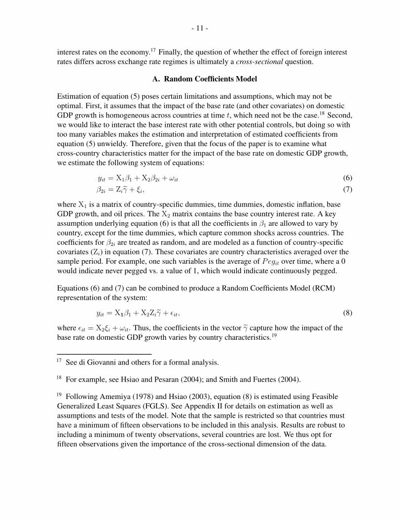
Estimation of equation (5) poses certain limitations and assumptions, which may not beoptimal. First, it assumes that the impact of the base rate (and other covariates) on domesticGDP growth is homogeneous across countries at time t, which need not be the case.18 Second,we would like to interact the base interest rate with other potential controls, but doing so withtoo many variables makes the estimation and interpretation of estimated coefficients fromequation (5) unwieldy. Therefore, given that the focus of the paper is to examine whatcross-country characteristics matter for the impact of the base rate on domestic GDP growth,we estimate the following system of equations:

yit = X1β1 + X2β2i + ωit (6)β2i = Ziγ + ξi, (7)

where X1 is a matrix of country-specific dummies, time dummies, domestic inflation, baseGDP growth, and oil prices. The X2 matrix contains the base country interest rate. A keyassumption underlying equation (6) is that all the coefficients in β1 are allowed to vary bycountry, except for the time dummies, which capture common shocks across countries. Thecoefficients for β2i are treated as random, and are modeled as a function of country-specificcovariates (Zi) in equation (7). These covariates are country characteristics averaged over thesample period. For example, one such variables is the average of Pegit over time, where a 0would indicate never pegged vs. a value of 1, which would indicate continuously pegged.

Equations (6) and (7) can be combined to produce a Random Coefficients Model (RCM)representation of the system:

yit = X1β1 + X2Ziγ + εit, (8)

where εit = X2ξi + ωit. Thus, the coefficients in the vector γ capture how the impact of thebase rate on domestic GDP growth varies by country characteristics.19

17 See di Giovanni and others for a formal analysis.

18 For example, see Hsiao and Pesaran (2004); and Smith and Fuertes (2004).

19 Following Amemiya (1978) and Hsiao (2003), equation (8) is estimated using FeasibleGeneralized Least Squares (FGLS). See Appendix II for details on estimation as well asassumptions and tests of the model. Note that the sample is restricted so that countries musthave a minimum of fifteen observations to be included in this analysis. Results are robust toincluding a minimum of twenty observations, several countries are lost. We thus opt forfifteen observations given the importance of the cross-sectional dimension of the data.

- 12 -

This econometric technique, along with our broad data set and multiple base rates, allows usto control for world growth effects with time controls, allows country specific responses tovariables such as oil prices and base country growth that may affect different countriesdifferently, and control for local inflation and unobserved country fixed effects. Such aspecification gives us far more power to isolate the impact of base interest rates on localeconomies than previous studies.

IV. DATA AND RESULTS

A. Data

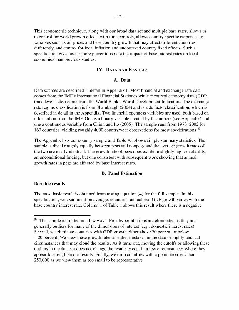
Data sources are described in detail in Appendix I. Most financial and exchange rate datacomes from the IMF’s International Financial Statistics while most real economy data (GDP,trade levels, etc.) come from the World Bank’s World Development Indicators. The exchangerate regime classification is from Shambaugh (2004) and is a de facto classification, which isdescribed in detail in the Appendix. Two financial openness variables are used, both based oninformation from the IMF. One is a binary variable created by the authors (see Appendix) andone a continuous variable from Chinn and Ito (2005). The sample runs from 1973–2002 for160 countries, yielding roughly 4000 country/year observations for most specifications.20

The Appendix lists our country sample and Table A1 shows simple summary statistics. Thesample is dived roughly equally between pegs and nonpegs and the average growth rates ofthe two are nearly identical. The growth rate of pegs does exhibit a slightly higher volatility;an unconditional finding, but one consistent with subsequent work showing that annualgrowth rates in pegs are affected by base interest rates.

B. Panel Estimation

Baseline results

The most basic result is obtained from testing equation (4) for the full sample. In thisspecification, we examine if on average, countries’ annual real GDP growth varies with thebase country interest rate. Column 1 of Table 1 shows this result where there is a negative

20 The sample is limited in a few ways. First hyperinflations are eliminated as they aregenerally outliers for many of the dimensions of interest (e.g., domestic interest rates).Second, we eliminate countries with GDP growth either above 20 percent or below−20 percent. We view these growth rates as either mistakes in the data or highly unusualcircumstances that may cloud the results. As it turns out, moving the cutoffs or allowing theseoutliers in the data set does not change the results except in a few circumstances where theyappear to strengthen our results. Finally, we drop countries with a population less than250,000 as we view them as too small to be representative.

- 13 -

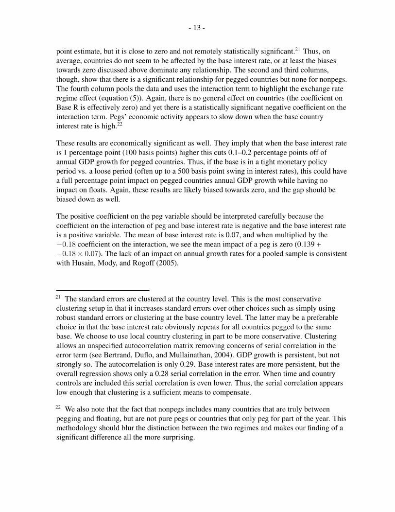
point estimate, but it is close to zero and not remotely statistically significant.21 Thus, onaverage, countries do not seem to be affected by the base interest rate, or at least the biasestowards zero discussed above dominate any relationship. The second and third columns,though, show that there is a significant relationship for pegged countries but none for nonpegs.The fourth column pools the data and uses the interaction term to highlight the exchange rateregime effect (equation (5)). Again, there is no general effect on countries (the coefficient onBase R is effectively zero) and yet there is a statistically significant negative coefficient on theinteraction term. Pegs’ economic activity appears to slow down when the base countryinterest rate is high.22

These results are economically significant as well. They imply that when the base interest rateis 1 percentage point (100 basis points) higher this cuts 0.1–0.2 percentage points off ofannual GDP growth for pegged countries. Thus, if the base is in a tight monetary policyperiod vs. a loose period (often up to a 500 basis point swing in interest rates), this could havea full percentage point impact on pegged countries annual GDP growth while having noimpact on floats. Again, these results are likely biased towards zero, and the gap should bebiased down as well.

The positive coefficient on the peg variable should be interpreted carefully because thecoefficient on the interaction of peg and base interest rate is negative and the base interest rateis a positive variable. The mean of base interest rate is 0.07, and when multiplied by the−0.18 coefficient on the interaction, we see the mean impact of a peg is zero (0.139 +−0.18× 0.07). The lack of an impact on annual growth rates for a pooled sample is consistentwith Husain, Mody, and Rogoff (2005).

21 The standard errors are clustered at the country level. This is the most conservativeclustering setup in that it increases standard errors over other choices such as simply usingrobust standard errors or clustering at the base country level. The latter may be a preferablechoice in that the base interest rate obviously repeats for all countries pegged to the samebase. We choose to use local country clustering in part to be more conservative. Clusteringallows an unspecified autocorrelation matrix removing concerns of serial correlation in theerror term (see Bertrand, Duflo, and Mullainathan, 2004). GDP growth is persistent, but notstrongly so. The autocorrelation is only 0.29. Base interest rates are more persistent, but theoverall regression shows only a 0.28 serial correlation in the error. When time and countrycontrols are included this serial correlation is even lower. Thus, the serial correlation appearslow enough that clustering is a sufficient means to compensate.

22 We also note that the fact that nonpegs includes many countries that are truly betweenpegging and floating, but are not pure pegs or countries that only peg for part of the year. Thismethodology should blur the distinction between the two regimes and makes our finding of asignificant difference all the more surprising.

- 14 -

Fixed effects and other controls

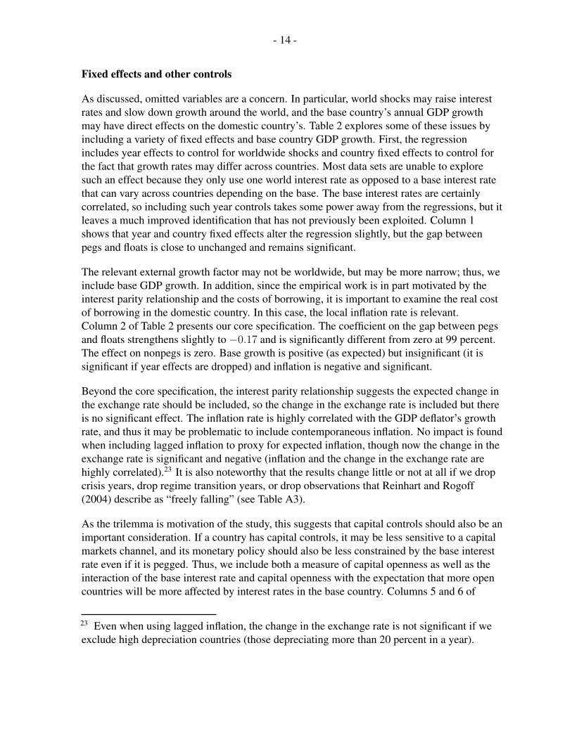
As discussed, omitted variables are a concern. In particular, world shocks may raise interestrates and slow down growth around the world, and the base country’s annual GDP growthmay have direct effects on the domestic country’s. Table 2 explores some of these issues byincluding a variety of fixed effects and base country GDP growth. First, the regressionincludes year effects to control for worldwide shocks and country fixed effects to control forthe fact that growth rates may differ across countries. Most data sets are unable to exploresuch an effect because they only use one world interest rate as opposed to a base interest ratethat can vary across countries depending on the base. The base interest rates are certainlycorrelated, so including such year controls takes some power away from the regressions, but itleaves a much improved identification that has not previously been exploited. Column 1shows that year and country fixed effects alter the regression slightly, but the gap betweenpegs and floats is close to unchanged and remains significant.

The relevant external growth factor may not be worldwide, but may be more narrow; thus, weinclude base GDP growth. In addition, since the empirical work is in part motivated by theinterest parity relationship and the costs of borrowing, it is important to examine the real costof borrowing in the domestic country. In this case, the local inflation rate is relevant.Column 2 of Table 2 presents our core specification. The coefficient on the gap between pegsand floats strengthens slightly to −0.17 and is significantly different from zero at 99 percent.The effect on nonpegs is zero. Base growth is positive (as expected) but insignificant (it issignificant if year effects are dropped) and inflation is negative and significant.

Beyond the core specification, the interest parity relationship suggests the expected change inthe exchange rate should be included, so the change in the exchange rate is included but thereis no significant effect. The inflation rate is highly correlated with the GDP deflator’s growthrate, and thus it may be problematic to include contemporaneous inflation. No impact is foundwhen including lagged inflation to proxy for expected inflation, though now the change in theexchange rate is significant and negative (inflation and the change in the exchange rate arehighly correlated).23 It is also noteworthy that the results change little or not at all if we dropcrisis years, drop regime transition years, or drop observations that Reinhart and Rogoff(2004) describe as “freely falling” (see Table A3).

As the trilemma is motivation of the study, this suggests that capital controls should also be animportant consideration. If a country has capital controls, it may be less sensitive to a capitalmarkets channel, and its monetary policy should also be less constrained by the base interestrate even if it is pegged. Thus, we include both a measure of capital openness as well as theinteraction of the base interest rate and capital openness with the expectation that more opencountries will be more affected by interest rates in the base country. Columns 5 and 6 of

23 Even when using lagged inflation, the change in the exchange rate is not significant if weexclude high depreciation countries (those depreciating more than 20 percent in a year).

- 15 -

Table 2 show a weak result in this direction. Using the Chinn-Ito variable, the point estimateis negative but not significant. Using a binary coding created by the authors yields a negativecoefficient significant at 90 percent.24

Subsamples

Table 3 shows the results across different sub-samples of the data. First, the results hold in thevery broad groupings of developing (LDC) and industrial countries (DC). In both cases, thereis a significant negative relationship for the interaction term of base interest rate and pegging.There is a small and weakly significant positive coefficient on the base rate for developingcountries in general, but this is most likely due to the omission of year effects.25 Dividingfurther by income groupings, there are strong significant reactions in high income, lowermiddle income, and lower income countries. The only grouping not to show expected resultsis the upper middle income. According to geographical groups, the results are strongest in theMiddle East, Europe, and sub-Saharan Africa. Importantly, no region has a significantcoefficient on the non-interacted base rate, so no region shows evidence of nonpegs beingaffected by the base rate. The results are not always significant as sample size shrinks, but itdoes not appear that they are driven by any one type of country or region, and they seem to berepresentative across a broad cross-section of countries.26

Alternate base interest rates

While the results appear robust to a variety of fixed effects, we continue to explore the results

24 Including further interactions (peg times capital openness and peg times capital opennessinteracted with the base rate) generates slightly stronger results on the interaction of capitalopenness and the base rate, but a positive coefficient on the peg times capital opennessinteracted with the base rate. Thus, capital openness and pegging are not purely additive nordo they both need to be active for an impact. A basic trilemma prediction would be thatpegging and capital openness only matter in conjunction, but the result we find is consistentwith Obstfeld and others (2005) results on interest rate effects.

25 We are unable to include year effects in these specifications because in some sub-samplesthere is insufficient variation in which country is the base. When we include year effects forthe developing sample, the positive coefficient on the base rate disappears while theinteraction term remains at −0.19 and is still significant.

26 Much of the previous work on this topic has focused on Latin America. We note that this isthe one region that comes close to having a significant reaction on the base interest rateregardless of exchange rate regime. In addition, if one does not exclude the very high inflationoutliers in this region and one does not control for inflation and base GDP growth, thecoefficient on base interest rate becomes significant, presenting a picture of all countries beingaffected by the base rate. Keeping high inflation countries in the full sample does not have thiseffect.

- 16 -

by taking further advantage of the fact that countries do not all peg to the same currency.Specifically, we check non-dollar based countries against the U.S. interest rate. If the onlyissue is a capital market effect, the dollar rate should be important, but if the effect is drivenby the monetary channel suggested by the trilemma, only the actual base interest rate shouldmatter. That is, if we see a gap between pegs and floats, does this gap exist for all largecountry interest rates, or only for the rate of the country to which they have pegged? Table 4shows that, in the core regression, dollar based countries and non-dollar based countries looksimilar, though the results are stronger for countries pegged to the dollar. Year effects cannotbe included in the dollar sample in column 1 because there is only one base interest rate used.Column 2 is the analogous regression for nondollar countries. Column 3 includes year effectsas well. When the U.S. interest rate is substituted for the base interest rate for the non-U.S.based countries, the only significant relationship is a positive coefficient on the non-interactedUS rate. This result is again likely due to the lack of year controls (this result is not apparentin many other specifications such as the one without country fixed effects shown in column 5.)There is no evidence, though, of a significant negative coefficient on the peg times theU.S. rate in any specification. Pegs do not respond negatively to the U.S. rate unless they arepegged to the dollar.

These regressions show that pegs are not simply more affected by large country interest rates,but are affected by the interest rates of their base in particular. Second, the fact that U.S. ratesdo not have a negative effect on non-U.S. based countries suggests that the capital marketeffect is not the primary channel. For almost any country, the U.S. interest rate is important infinancial markets, but, pegs only respond to their base, not to the dollar interest rate.

Other controls and robustness checks

Including more controls and characteristics increases the number of interaction and crossinteraction terms required such that the results are less straightforward to interpret. The RCMframework is thus exploited to explain the reaction of countries’ growth rate to the baseinterest rate using a number of different institutional and country characteristics ranging fromthe exchange rate regime to capital controls to trade levels.

Before turning to these results, we briefly summarize other controls and estimation issues wehave considered. First, we have run regressions using a dynamic specification of equation (5).In particular, we include lagged domestic GDP growth. There is very little difference in theresults, most likely because output growth is not necessarily a very persistent variable (unlikethe level of GDP, for example). Real interest rates are used instead of nominal interest rates.While the rate that is relevant in interest parity or other international conditions is the nominalrate, we also examine base real interest rates. Results vary depending on how the base realinterest rate is defined (subtracting current or lagged inflation from the nominal rate).Alternatively, including the base interest rate and base inflation separately continues to giveour standard results. In addition, regressions are conducted across subsets of countries dividedby debt levels. Least indebted countries appear to be the least exposed to foreign interest

- 17 -

rates, yet the core result of pegs reacting more than floats appears to hold across quartiles bydebt level, though the significance varies.

In addition, since we discuss borrowing costs as a potential channel, we check that our resultshold for real investment growth in addition to real GDP growth. Results (see Table A2) areeven stronger than our main results in both size and significance. Again, there is a strongdifference between pegs and nonpegs. Pegs exhibit a strong negative response in realinvestment growth rates after a base interest rate increase. And, again, non-dollar pegs do notrespond to dollar interest rates despite responding quite strongly to their own base countryinterest rates.

Finally, other exchange rate regime classifications are examined. Replicating Table 1 usingde jure codes (countries’ declared regime status), shows directionally similar but weakerresults (see columns 5 and 6 of Table A4). This is not surprising given the fact that some ofthe observations are miscoded in the de jure codes mixing pegs and floats together. UsingReinhart and Rogoff’s classification codes (condensed to a binary coding) yields similar,though weaker, results without fixed effects and controls, and opposite reactions with fulleffects and controls (the base rate is weakly significantly negative and the interaction term isinsignificant). When restricting the sample to the 80 percent of the observations where theReinhart and Rogoff and Shambaugh classifications agree, the results are similar withouteffects and unclear with the effects. As columns 1 and 2 show, a significant number ofobservations are lost when using Reinhart and Rogoff codes. Furthermore, their codes showfewer switches making finding significant results with country fixed effects less likely.Finally, we use the disaggregated Reinhart and Rogoff codes as well (see Table A5). Here,with no fixed effects or controls, only pegs have a significant relationship with the baseinterest rate and only crawling pegs have strongly significant reactions with fixed effects. Theresults for floating countries and freely falling countries are always close to zero and notremotely significant. Thus, the reactions are not identical across classifications, but they aresimilar in a number of specifications.27

C. Random Coefficients Estimation

We next turn to results from estimating equation (8). As discussed above, using a randomcoefficients framework provides a method that not only allows for greater flexibility inestimating the impact of the base interest rate on domestic annual GDP growth using the timeseries data while controlling for global shocks, but also allows us to take into account manycross-country controls when trying to explain this impact of the base interest rate.

27 We see an advantage in using the Shambaugh classification based on data coverage,availability, and the annual nature of the coding used which matches the frequency of ourother analysis and data. Thus, we use it for the bulk of our analysis. See Shambaugh (2004)for an extensive discussion of the different classifications.

- 18 -

This estimation methodology confirms the importance of the exchange rate regime. Inparticular, Table 5 presents the estimated coefficients for the whole sample and the lessdeveloped country sub-sample, respectively.28 The country-specific variables used in theregressions (i.e., the X1 variables) include a constant, domestic inflation, base GDP growth,and the oil price. Furthermore, a time effect is included for all countries. We alsoexperimented with including exchange rate changes, but, like in the panel estimation,including this variable does very little to our estimates.

Before turning to the precise quantitative results, the main result can be summarized inFigure 1. The vertical axis represents estimated coefficients of the impact of the base rate onannual GDP growth, and are calculated from a first-step estimation of a FGLS procedure (seethe Appendix for details). The horizontal axis represents how pegged a country was over thesample; i.e., it is an average of the exchange rate regime binary indicator over the period. Avalue of zero implies that the country was always a nonpeg, while a one indicates that countryalways fixed to its base. The figure depicts a negative relationship, implying that the averageimpact of a foreign interest rate on domestic real annual GDP growth will be larger the morefixed a country is on average.

Table 5 shows that this result is robust across all specifications, and is both economically andstatistically significant. The core result in column 1 indicates that foreign interest rates being1 percentage point higher result in a 0.30 percentage point greater impact on annual real GDPgrowth for countries that were pegged throughout the sample compared to those that werefloating, while the impact is 0.29 percentage points for the less developed country sample.This result is even larger than in the panel regressions now that multiple countrycharacteristics are included. Given that base country interest rates can move by up to500 basis points over a cycle, it suggests a very large impact on pegs versus floats. Theinclusion of several controls and the high statistical significance of the peg coefficient inTable 5 indicates that the results are robust. Interestingly, the majority of other controlvariables are not significant. However, it is worth noting that the sign of the coefficients ingeneral line up with what one would expect.

First, the Trade/GDP coefficient is generally negative indicating that foreign interest rateshave a larger impact for economies that are open to trade. There is no a priori reason toexpect this result, but trade and financial openness are strongly correlated, and morefinancially open countries may be impacted more by foreign interest rates. Second, the impactof the base rate on domestic output growth is weaker the more a country exports to its basecountry (as a ratio of GDP), which makes sense given the identification problem resulting

28 Results were broadly consistent for the developed country sub-sample, but statisticalsignificance is lower given a smaller cross-sectional component. Results are available fromthe authors upon request.

- 19 -

from the forward-looking bias of the foreign monetary policymaker and common shocks.29

This result is significant in columns 5 and 6.30 Income variables are not significant, except forcolumns 5 and 6, where low income countries appear to be positively affected, though due tothe inclusion of other variables, there are very few low income countries left in the sample inthese specifications. Finally, the capital control variable (KA open) is never significant and thepoint estimate is practically zero. We have experiment with other capital controls data(Chinn-Ito), and have not found any strong results for this indicator, though the peg variableremains strong.

Financial markets, both domestic and international, may also affect how strongly the domesticeconomy reacts to movements in the base rate. We therefore examine the impact of theaverage level of financial development, external capital flows, and financial openness. Onlythe ratio of credit to GDP in column 4 is significant, and has it a positive coefficient, indicatingthat the base rate has a smaller impact in more financially developed economy (viz. credit).31

D. Channels

Foreign interest rates should not have a direct effect on the domestic economy. However, theymay operate through some channel and have an indirect impact either by affecting domesticinterest rates, investment flows, or other variables that contribute to annual GDP growth. Inmany ways, the channels have already been tested by examining characteristics and baserates. Our results that pegs are more affected than floats is consistent with an interest ratechannel. The lack of an effect of the U.S. interest rate on both pegs and floats that are based tocountries other than the U.S. is inconsistent with a strong capital market channel. Similarly,the fact that the exchange rate regime is the most dominant characteristic driving therelationship between base rates and GDP growth in the RCM framework is again consistentwith the interest rate channel.

To further determine through which channel(s) the foreign interest rate operates, we test aseries of variables against the base interest rate and see if they move in a direction consistentwith the direction that GDP growth moves. If there is no relationship between a particularvariable and the base interest rate, this suggests that the channel is not operational. Finding

29 Note that we also control for this effect in the time series part of the estimation byincluding base GDP growth in X1.

30 It is also interesting to note that the coefficient on the peg increases (in absolute terms)when including the exports to base variable (the specification with only the peg is notreported, but is available upon request).

31 This result points to a potential dampening effect of financial depth on the impact of thebase interest rate on annual output growth. This dampening effect of financial depth has beenhighlighted in recent work by Aghion and others (2005).

- 20 -

significant relationships does not establish that a channel is the primary one affectingdomestic growth definitively, however, but establishes the existence of a potential channel.

This methodology is analogous to that of Kim (2001), who applies the same identificationstrategies he uses to identify the impact of monetary policy on output to other channelvariables (e.g., trade). He then asks what models the resulting impulses of these variables areconsistent with. We do not follow a VAR strategy to identify monetary shocks, but we expectthat the impact of base interest rates on economic variables to differ given potential channels,as well as across different exchange rate regimes.

Interest rate channel

We consider a wide variety of potential channels. As noted often in the paper, one focus is onthe direct effect of base interest rates on domestic interest rates. The presumption is thatdomestic interest rates have some impact on the economy, and if movements in base interestrates force movements in the local rate, this will have an impact on the economy. Thus, wetest the impact of changes in base interest rates on domestic rates.

This channel has been tested in Shambaugh (2004) and Obstfeld, Shambaugh, and Taylor(2004 and 2005) with a series of controls and robustness checks. We do not repeat all testshere but simply check the basic specifications with our data.32 Table 6 shows that domesticrates do seem to move with base interest rates, but this is driven by pegs. There is no effect onfloats, but the peg interaction term shows a statistically significant and economicallymeaningful coefficient of roughly 0.4 depending on the specification, implying that 40 percentof base rate changes are passed through to domestic rates in fixed exchange rate countries.33

Thus, the direct monetary channel appears to be a possible explanation for the growth impact.When base interest rates rise, domestic rates in pegged countries rise. The direction anddifference between pegs and nonpegs are consistent with our growth results.

32 Shambaugh (2004) discusses the fact that we should be worried about persistence innominal interest rates and should consider a specification in differences. We follow that here.Domestic rates are far more persistent than the other variables we consider for channels, thatis why we turn to differences only for the interest rate and spreads regressions.

33 These results are also consistent with findings in Miniane and Rogers (2003) who find thatlocal interest rates respond to base interest rates more for pegs. Borensztein, Zettelmeyer, andPhilippon (2001) also find pegs respond more to monetary shocks when looking at a smallgroup of countries. Frankel, Schmukler, and Serven (2004) agree that short-run reactions areslower in nonpegs than in pegs, though they argue that long run reactions are more similar(cf Shambaugh). Finally, Hausmann and others (1999) do not find this relationship whenusing a small panel of Latin American countries and using real interest rates.

- 21 -

Interest rate gap channel

Alternatively, the foreign interest rate may not only move the domestic rate directly, but alsohave an impact on the spread. Consider the equation:

Rit = Rbit + ∆eit + δit, (9)

where Rit is the local rate, ∆eit is the expected change in the exchange rate, and δit is arelative risk premium on domestic vs. foreign assets. The change in the base rate may notsimply affect the domestic rate directly, but it may also change expectations on the exchangerate and the risk premium causing a change in the spread between the domestic and foreignrates. Uribe and Yue (2005) note that an increase in the base rate might not only increase thedomestic rate directly, but may also increase the spread generating the possibility of a morethan one for one increase in domestic rates.34 We thus test the impact of the base rate on thespread between domestic and base rates.35

Examining the interest rate gap (defined as the domestic minus the base interest rate) and thebase interest rate yields statistically significant results, but the direction of the reactions wouldnot explain a decrease in GDP growth after an increase in base rates. Column 2 of Table 6shows the results. There is a strongly negative reaction implying that the spread declines afteran increase in base interest rates, and this reaction is stronger for nonpegs. This result is notsurprising. If the domestic rate does not respond to the base rate in floating countries, ascolumn 1 shows, then the spread automatically moves opposite the base interest rate. Thespread shifts less for pegs because domestic interest rates do go up with the base interest rateto some extent in these countries. A declining spread should be positively correlated withGDP growth, but there is no improvement in GDP after a base rate increase. Thus, theseresults seem to imply there is not a strong spreads channel largely because for most countries,there is no affect of base interest rates on domestic rates, and the spread is not acting like amultiplier of base rate changes, but is simply the residual arising from domestic rates notmoving with the base rate fully.36

34 They find that the U.S. rate and the spread can explain up to 20 percent of domesticaggregate activity. However, the standard error bands on the output response to U.S. interestrate changes generally include zero and the sample size is restricted for data reasons. See alsoNeumeyer and Perri (2005). They examine the volatility of business cycles in five emergingeconomies, discern that real interest rate volatility contributes to the volatility of the cycle,and that both foreign rates and country risk contribute to the volatility of the real rate.

35 Note that Uribe and Yue (2005) look at foreign currency denominated bonds, so theirspread is strictly δit , whereas our interest rates are domestic, so our spread is δit + ∆eit.

36 These results are almost identical if one looks at the the spread rather than the change in thespread itself. The only difference being that the difference between pegs and nonpegsbecomes less significant. We use differences because spreads, like domestic interest rates, arequite persistent.

- 22 -

Exports to base channel

The base country interest rate may also have real effects in the base country. To the extent thatsome countries are economically dependent on the base country, a primary channel throughwhich this may have a direct effect on the domestic GDP growth is changes in exports to thebase country. There are two reasons to be somewhat skeptical that this channel will havestrong effects, however. First, to the extent that interest rates in the base countries arecounter-cyclical, one would expect the classic monetary policy result that high rates aresimply offsetting higher expected growth, and not actually slowing the economy down torecession levels. Thus, it would be surprising to see an impact through the growth rates of thebase economy. In addition, base country GDP growth has been included in the output growthregressions, and it does not weaken the base interest rate effect. Still, we test here the impactof base rates on exports to the base country to see if there is a possibility of such a channel.

Table 7 column 1 shows that exports to the base do not move in a direction consistent with ourresults. Nonpegs’ exports are unaffected, but there is a weakly significant increase in exportsto the base by pegs. This result fits the theory that base countries may be actingcounter-cyclically and this counter-cyclicality may in fact be mitigating our main results. Itappears that pegs are helped by an increase in exports to the base when the base rate is high,but that this relationship is overwhelmed by the monetary channel.37

Capital flows channel

Calvo, Leiderman, and Reinhart (1993 and 1996) consider the impact of large country interestrates on financial flows. Their concern is that interest rate movements in developed countriesmay affect the volume of capital flows to developing countries. The hypothesis is that anincrease (decrease) in base interest rates would shrink (expand) the pool of capital availableoutside the base country because more base country funds would stay (leave) home. Thus, wetest the impact of base interest rates on domestic country financial flows. There is no a priorireason for this effect to differ across exchange rate regime.

Table 7 columns 2 and 3 show the effect of the base rate on capital flows. Two indicators ofthe impact are considered. The first is the percentage change in total external liabilitiesagainst the base rate. The second is the change in total liabilities to GDP. In general, theresults do not support a capital flows channel. The change in external liabilities does not show

37 The exports to base/GDP series is quite persistent as well, suggesting the possibility ofusing changes for this channel as well. When changes in exports to base (divided by GDP) areregressed on changes in the base interest rate, there is no significant coefficient on theinteraction, but the non-interacted base interest rate coefficient is now small and weaklysignificant positive coefficient implying that the boost in exports that comes with growingbase countries may hit pegs and nonpegs alike. Regardless, this does not seem to be a channelthat explains slower growth when base interest rates are high.

- 23 -

a relationship in either specification.38 Thus, it does not appear that the base interest ratesignificantly affects capital flows into these countries. The point estimates are negative, butthere is no statistically significant evidence supporting a capital flows channel.

Exchange rate change channel

The base interest rate will potentially move the domestic exchange rate and hence affect theeconomy through an exchange rate change channel. An increase in the base rate may causethe base currency to appreciate against all other currencies (that float) meaning that anyfloating country will depreciate against the base. Thus, we test the nominal exchange raterelative to the base country against the base interest rate. Table 7, column 4 shows the results.There are no significant reactions to the base interest rate. The peg and domestic inflation arethe only significant variables. We see that pegs tend to appreciate (a negative coefficient)relative to nonpegs though country fixed effects as well as the constant and other controlsobscure the exact pattern. Given the insignificant reaction to the base interest rate, though, thisdoes not appear to be a primary channel.

Thus, while these explorations of the channels are not intended to be definitive on any onerelationship measured, the one effect that seems to both run in the direction that would slowannual growth and differ significantly by exchange rate regime is the impact of base rates ondomestic interest rates. This finding does not establish it as the only channel, but it seems tobe an important one.

V. CONCLUSION

This paper shows that while interest rates in large countries may have an effect on othercountries’ real economies, this impact only exists for pegged countries. Countries without afixed exchange rate show no relationship between annual real GDP growth and the baseinterest rate, but countries with a fixed exchange rate grow between 0.1 to 0.2 percentagepoints slower when base interest rates are 1 percentage point higher. The results appear robustto a wide variety of controls and specifications. Controlling for time, region, income,base-country GDP growth, and other controls all present the same picture. In addition, peggedcountries do not respond to any world interest rate, but only the rate of the country to whichthey peg—further suggesting the importance of the peg in this relationship. We have exploitedvariation in base rates and used RCM techniques to achieve better identification and increaseconfidence in the robustness of the results.

Our work on channels suggests that the effect of base rates on domestic interest rates inpegged countries is the primary channel through which this impact on GDP takes place.Pegged countries move their interest rates with the base-country interest rates while floats donot. On the other hand, there does not seem to be a robust relationship consistent with thedirection that growth moves between the base-country interest rate and numerous other

38 We have also experimented with examining changes in the base rates and results are similar.

- 24 -

potential channels such as the exchange rate, capital flows, and the interest rate spread overthe base country.

While the fact that fixed-exchange-rate countries’ growth rates move with the base interestrate matches our theoretical predictions, the results are surprising on two levels. First, the lackof a reaction in the floating countries runs counter to conventional wisdom regarding theextent to which large-country interest rates affect the rest of the world. Second, with thefindings that the primary channel is the direct monetary policy channel, we add to ourunderstanding of how and why large-country interest rates matter for pegs and demonstratethat exogenous monetary policy can have a palpable effect on the economy.

For many years, economists have struggled with the difficulty of finding robustmacroeconomic relationships that vary across exchange rate regime. Recently, there has beenadditional work suggesting that monetary policy autonomy, growth, inflation, and trade mayall vary with the exchange rate regime, at least to some extent. Stretching back further, Floodand Rose (1995) found a negative relationship between the exchange rate and outputvariability. The results here suggest that being forced to follow the base-country’s monetarypolicy even when it is not optimal for the domestic economy may cause increased volatility inGDP for fixed exchange rate countries.

These results do not suggest that pegging is either a good or bad idea, but instead add to thecalculus of costs and benefits (in this case costs) an economy will face when it fixes itsexchange rate. Furthermore, our results suggest that losing monetary autonomy when pegginghas real impacts on the economy. Obviously, by floating, a country may expose itself tovolatility owing to changes in the nominal exchange rate, but pegging does not eliminatevolatility. Pegging forces a country’s interest rates to follow the base-country rates, which maygenerate more volatility in GDP by eliminating countercyclical monetary policy as an option.

- 25 - APPENDIX I

I. DATA

The exchange rate regime classification comes from Shambaugh (2004) and is described therein detail. In short, a country is classified as pegged if its official nominal exchange rate stayswithin ±2 percent bands over the course of the year against the base country. The basecountry is chosen based on the declared base, the history of a countries’ exchange rate, bycomparing its exchange rate to a variety of potential bases, and by looking at regionaldominant currencies. In addition, single year pegs are eliminated as they more likely representa random lack of variation rather than a true peg. Finally, realignments, where a countrymoves from one peg level to another with an otherwise constant exchange rate are alsoconsidered pegs. Nonpegs are also assigned a base determined by the country they peg towhen they are pegging at other times in the sample. While we typically use the term “nonpeg”and the more colloquial “float” interchangeably, any country/year observation not coded as apeg is considered a nonpeg, so they are not all pure floats, but include all sorts of nonpeggedregimes. Shambaugh makes extensive comparisons of this methodology and otherclassifications. The de jure measure is based on the IMF Annual Report on Exchange RateArrangements and Exchange Restrictions compiled in Shambaugh and extended by theauthors. The Reinhart-Rogoff classification is from Reinhart and Rogoff (2004) and isavailable on Carmen Reinhart’s website. Their coding uses parallel market data and assessesthe conditional probability an exchange rate will move outside a certain range over a five-yearwindow. See Reinhart and Rogoff (2004) for more detail. In some specifications, we collapsethe five-way classification into a binary one, considering all observations that are not codedpegs as nonpegs.

There are two financial openness variables used. One is the financial openness variable asdefined by Chinn and Ito (2005). This is a continuous index based on information across fourmajor categories of restrictions in the IMF Annual Report on Exchange Rate Arrangementsand Exchange Restrictions. The other variable, is a binary indicator created by the authorsbased on data from the IMF Annual Report on Exchange Rate Arrangements and ExchangeRestrictions line E2, which signifies “restrictions on payments for capital transactions.” For1973–95, we begin with data provided by Gian Maria Milesi-Ferretti and augment it with datafrom Shambaugh (2004). After 1995, the IMF stopped reporting this series and reporteddisaggregated information. The series is extended for 1996–2002 using changes in thedisaggregated coding and descriptions in the yearbook to determine changes in the binarycodes. Shambaugh discusses the coding in more detail including the fact that this series ishighly correlated with other more detailed or disaggregated measures.

Our financial flows and debt variables are updated data from Lane and Milesi-Ferretti (2001).The Credit/GDP variable is defined as private credit by banks and other Financial institutionsto GDP, and comes from the updated financial Development and Structure database of Beck,Demirguc-Kunt, and Levine (1999), which can be found at http://econ.worldbank.org.

The rest of the macroeconomic data come from standard sources. Real GDP, oil prices,M2/GDP, Trade/GDP, income levels, and regional and income dummies come from the World

- 26 - APPENDIX I

Development Indicators database of the World Bank. Exchange Rates and inflation comefrom the International Monetary Fund’s International Financial Statistics database. Interestrates are from the IFS as well as Datastream and Global Financial Database. Exports to thebase country are derived from the IMF Direction of Trade Statistics.

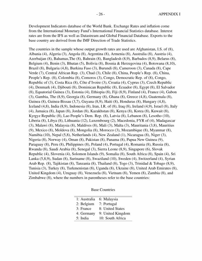
The countries in the sample whose output growth rates are used are Afghanistan, I.S. of (8),Albania (4), Algeria (3), Angola (8), Argentina (8), Armenia (8), Australia (8), Austria (4),Azerbaijan (8), Bahamas,The (8), Bahrain (8), Bangladesh (8,9), Barbados (8,9), Belarus (8),Belgium (4), Benin (3), Bhutan (5), Bolivia (8), Bosnia & Herzegovina (4), Botswana (8,10),Brazil (8), Bulgaria (4,8), Burkina Faso (3), Burundi (8), Cameroon (3), Canada (8), CapeVerde (7), Central African Rep. (3), Chad (3), Chile (8), China, People’s Rep. (8), China,People’s Rep. (8), Colombia (8), Comoros (3), Congo, Democratic Rep. of (8), Congo,Republic of (3), Costa Rica (8), Cote d’Ivoire (3), Croatia (4), Cyprus (3), Czech Republic(4), Denmark (4), Djibouti (8), Dominican Republic (8), Ecuador (8), Egypt (8), El Salvador(8), Equatorial Guinea (3), Estonia (4), Ethiopia (8), Fiji (8,9), Finland (4), France (4), Gabon(3), Gambia, The (8,9), Georgia (8), Germany (8), Ghana (8), Greece (4,8), Guatemala (8),Guinea (8), Guinea-Bissau (3,7), Guyana (8,9), Haiti (8), Honduras (8), Hungary (4,8),Iceland (4,8), India (8,9), Indonesia (8), Iran, I.R. of (8), Iraq (8), Ireland (4,9), Israel (8), Italy(4), Jamaica (8), Japan (8), Jordan (8), Kazakhstan (8), Kenya (8), Korea (8), Kuwait (8),Kyrgyz Republic (8), Lao People’s Dem. Rep. (8), Latvia (8), Lebanon (8), Lesotho (10),Liberia (8), Libya (8), Lithuania (12), Luxembourg (2), Macedonia, FYR of (4), Madagascar(3), Malawi (8), Malaysia (8), Maldives (8), Mali (3), Malta (3), Mauritania (3,8), Mauritius(9), Mexico (8), Moldova (8), Mongolia (8), Morocco (3), Mozambique (8), Myanmar (8),Namibia (10), Nepal (5,8), Netherlands (4), New Zealand (1), Nicaragua (8), Niger (3),Nigeria (8), Norway (4), Oman (8), Pakistan (8), Panama (8), Papua New Guinea (9),Paraguay (8), Peru (8), Philippines (8), Poland (4), Portugal (4), Romania (8), Russia (8),Rwanda (8), Saudi Arabia (8), Senegal (3), Sierra Leone (8,9), Singapore (6), SlovakRepublic (4), Slovenia (4), Solomon Islands (9), Somalia (8), South Africa (8), Spain (4), SriLanka (5,8,9), Sudan (8), Suriname (8), Swaziland (10), Sweden (4), Switzerland (4), SyrianArab Rep. (8), Tajikistan (8), Tanzania (8), Thailand (8), Togo (3), Trinidad & Tobago (8,9),Tunisia (3), Turkey (8), Turkmenistan (8), Uganda (8), Ukraine (8), United Arab Emirates (8),United Kingdom (4), Uruguay (8), Venezuela (8), Vietnam (8), Yemen (8), Zambia (8), andZimbabwe (8), where the numbers in parentheses refer to the base countries:

Base Countries

1: Australia 6: Malaysia2: Belgium 7: Portugal3: France 8: United States4: Germany 9: United Kingdom5: India 10: South Africa

- 27 - APPENDIX II

II. ESTIMATION OF RCM MODEL

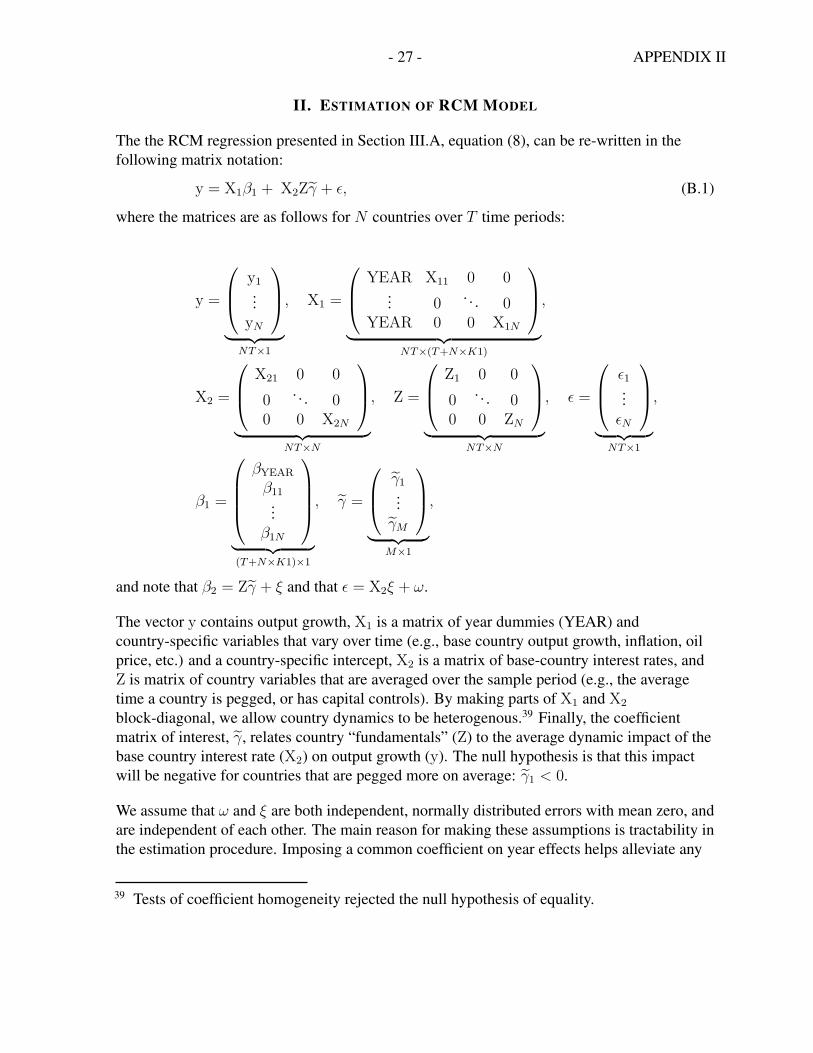
The the RCM regression presented in Section III.A, equation (8), can be re-written in thefollowing matrix notation:

y = X1β1 + X2Zγ + ε, (B.1)

where the matrices are as follows for N countries over T time periods:

y =

y1...

yN

︸ ︷︷ ︸NT×1

, X1 =

YEAR X11 0 0... 0

. . . 0YEAR 0 0 X1N

︸ ︷︷ ︸NT×(T+N×K1)

,

X2 =

X21 0 0

0. . . 0

0 0 X2N

︸ ︷︷ ︸NT×N

, Z =

Z1 0 0

0. . . 0

0 0 ZN

︸ ︷︷ ︸NT×N

, ε =

ε1...

εN

︸ ︷︷ ︸NT×1

,

β1 =

βYEAR

β11...

β1N

︸ ︷︷ ︸(T+N×K1)×1

, γ =

γ1...

γM

︸ ︷︷ ︸M×1

,

and note that β2 = Zγ + ξ and that ε = X2ξ + ω.

The vector y contains output growth, X1 is a matrix of year dummies (YEAR) andcountry-specific variables that vary over time (e.g., base country output growth, inflation, oilprice, etc.) and a country-specific intercept, X2 is a matrix of base-country interest rates, andZ is matrix of country variables that are averaged over the sample period (e.g., the averagetime a country is pegged, or has capital controls). By making parts of X1 and X2

block-diagonal, we allow country dynamics to be heterogenous.39 Finally, the coefficientmatrix of interest, γ, relates country “fundamentals” (Z) to the average dynamic impact of thebase country interest rate (X2) on output growth (y). The null hypothesis is that this impactwill be negative for countries that are pegged more on average: γ1 < 0.

We assume that ω and ξ are both independent, normally distributed errors with mean zero, andare independent of each other. The main reason for making these assumptions is tractability inthe estimation procedure. Imposing a common coefficient on year effects helps alleviate any

39 Tests of coefficient homogeneity rejected the null hypothesis of equality.

- 28 - APPENDIX II

cross-country correlation arising from global shocks in the ω vector.40 Furthermore, includingthese dummies and the impact of oil prices also helps alleviate autocorrelation in the errors ofω.41 By forcing ξ to be distributed independently across sections and homoscedastic, we areassuming that the β2,i’s are uncorrelated across countries, and have a constant variance.Inspection and tests of the covariance matrix of equation (7) indicate that these are reasonableassumptions to make. Finally, assuming that ω and ξ are independent implicitly assumes thatthe dynamic and cross-sectional error structures are uncorrelated, which is standard in panelanalysis. Many of these assumptions can be relaxed by using GMM estimation techniques,but would result in a loss of efficiency.

Given the assumptions made on the error structure, one can easily apply a two-step FGLSestimation technique based on Amemiya (1978), and found in Hsiao (2003). In particular, firstregress y on X1 and X2 and calculate a variance-covariance matrix, Σ1. Next, take theestimated country-specific base rate coefficients, β2i, and regress these on Z to produce OLSestimates of γ, γOLS .42 The variance-covariance matrix, Σ2, of these estimates is thencalculated taking into account the uncertainty of the estimated base rate coefficients from thefirst regression. The final output of this first-step procedure is a total variance-covariancematrix, which is the sum of the two variance-covariance matrices (Σ1 + Σ2) and is blockdiagonal. This matrix captures the uncertainty of the estimated β and γ coefficients. Thesecond-step of the procedure is to estimate equation (B.1) by weighting with this totalvariance-covariance matrix. This estimation produces the most efficient estimates of γ, γGLS ,and β1, β1GLS .

40 See Hsiao and Pesaran (2004), Section 9, on the difficulties of modeling cross-sectioncorrelation when N is large (> 10) and for a discussion on other possible ways to modelcross-section correlation in a RCM set-up. Note that a SURE framework would not worksince N > T in our sample. Furthermore, including common year effects greatly alleviatescross-sectional correlation as in the panel regressions according to the test statistics developedby Pesaran (2004).

41 See the discussion on the panel results in footnote 21.

42 It is these estimated γ that are plotted against the average peg variables (Z1) in Figure 1.

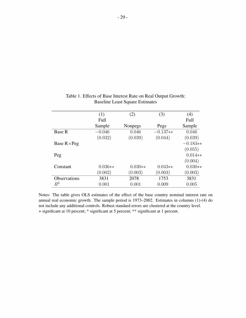
- 29 -

Table 1. Effects of Base Interest Rate on Real Output Growth:Baseline Least Square Estimates

(1) (2) (3) (4)Full Full

Sample Nonpegs Pegs SampleBase R −0.046 0.046 −0.137∗∗ 0.046

(0.032) (0.039) (0.044) (0.039)Base R×Peg −0.183∗∗

(0.055)Peg 0.014∗∗

(0.004)Constant 0.036∗∗ 0.030∗∗ 0.043∗∗ 0.030∗∗

(0.002) (0.003) (0.003) (0.003)Observations 3831 2078 1753 3831R2 0.001 0.001 0.009 0.005

Notes: The table gives OLS estimates of the effect of the base country nominal interest rate onannual real economic growth. The sample period is 1973–2002. Estimates in columns (1)-(4) donot include any additional controls. Robust standard errors are clustered at the country level.+ significant at 10 percent; * significant at 5 percent; ** significant at 1 percent.

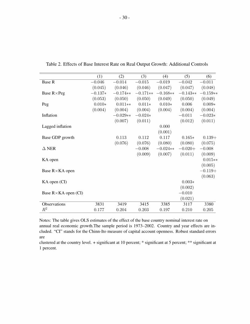
- 30 -

Table 2. Effects of Base Interest Rate on Real Output Growth: Additional Controls

(1) (2) (3) (4) (5) (6)Base R −0.046 −0.014 −0.015 −0.019 −0.042 −0.011

(0.045) (0.046) (0.046) (0.047) (0.047) (0.048)Base R×Peg −0.137∗ −0.174∗∗ −0.171∗∗ −0.168∗∗ −0.143∗∗ −0.159∗∗

(0.053) (0.050) (0.050) (0.049) (0.050) (0.049)Peg 0.010∗ 0.011∗∗ 0.011∗ 0.010∗ 0.006 0.009∗

(0.004) (0.004) (0.004) (0.004) (0.004) (0.004)Inflation −0.029∗∗ −0.024∗ −0.011 −0.023∗

(0.007) (0.011) (0.012) (0.011)Lagged inflation 0.000

(0.001)Base GDP growth 0.113 0.112 0.117 0.165∗ 0.139+

(0.076) (0.076) (0.080) (0.080) (0.075)∆ NER −0.008 −0.024∗∗ −0.020+ −0.008

(0.009) (0.007) (0.011) (0.009)KA open 0.015∗∗

(0.005)Base R×KA open −0.119+

(0.063)KA open (CI) 0.003∗

(0.002)Base R×KA open (CI) −0.010

(0.021)Observations 3831 3419 3415 3385 3117 3380R2 0.177 0.204 0.203 0.197 0.210 0.205

Notes: The table gives OLS estimates of the effect of the base country nominal interest rate onannual real economic growth.The sample period is 1973–2002. Country and year effects are in-cluded. “CI” stands for the Chinn-Ito measure of capital account openness. Robust standard errorsareclustered at the country level. + significant at 10 percent; * significant at 5 percent; ** significant at1 percent.

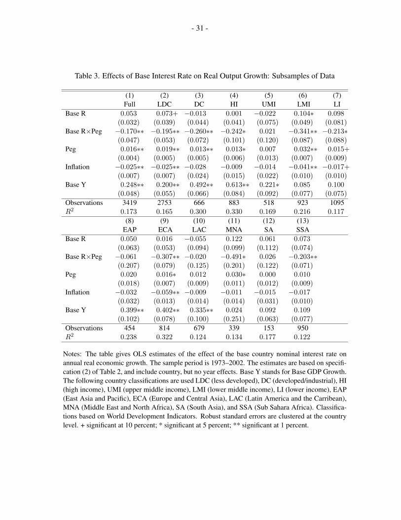
- 31 -

Table 3. Effects of Base Interest Rate on Real Output Growth: Subsamples of Data

(1) (2) (3) (4) (5) (6) (7)Full LDC DC HI UMI LMI LI

Base R 0.053 0.073+ −0.013 0.001 −0.022 0.104∗ 0.098(0.032) (0.039) (0.044) (0.041) (0.075) (0.049) (0.081)

Base R×Peg −0.170∗∗ −0.195∗∗ −0.260∗∗ −0.242∗ 0.021 −0.341∗∗ −0.213∗(0.047) (0.053) (0.072) (0.101) (0.120) (0.087) (0.088)

Peg 0.016∗∗ 0.019∗∗ 0.013∗∗ 0.013∗ 0.007 0.032∗∗ 0.015+(0.004) (0.005) (0.005) (0.006) (0.013) (0.007) (0.009)

Inflation −0.025∗∗ −0.025∗∗ −0.028 −0.009 −0.014 −0.041∗∗ −0.017+(0.007) (0.007) (0.024) (0.015) (0.022) (0.010) (0.010)

Base Y 0.248∗∗ 0.200∗∗ 0.492∗∗ 0.613∗∗ 0.221∗ 0.085 0.100(0.048) (0.055) (0.066) (0.084) (0.092) (0.077) (0.075)

Observations 3419 2753 666 883 518 923 1095R2 0.173 0.165 0.300 0.330 0.169 0.216 0.117

(8) (9) (10) (11) (12) (13)EAP ECA LAC MNA SA SSA

Base R 0.050 0.016 −0.055 0.122 0.061 0.073(0.063) (0.053) (0.094) (0.099) (0.112) (0.074)

Base R×Peg −0.061 −0.307∗∗ −0.020 −0.491∗ 0.026 −0.203∗∗(0.207) (0.079) (0.125) (0.201) (0.122) (0.071)

Peg 0.020 0.016∗ 0.012 0.030∗ 0.000 0.010(0.018) (0.007) (0.009) (0.011) (0.012) (0.009)

Inflation −0.032 −0.059∗∗ −0.009 −0.011 −0.015 −0.017(0.032) (0.013) (0.014) (0.014) (0.031) (0.010)

Base Y 0.399∗∗ 0.402∗∗ 0.335∗∗ 0.024 0.092 0.109(0.102) (0.078) (0.100) (0.251) (0.063) (0.077)

Observations 454 814 679 339 153 950R2 0.238 0.322 0.124 0.134 0.177 0.122

Notes: The table gives OLS estimates of the effect of the base country nominal interest rate onannual real economic growth. The sample period is 1973–2002. The estimates are based on specifi-cation (2) of Table 2, and include country, but no year effects. Base Y stands for Base GDP Growth.The following country classifications are used LDC (less developed), DC (developed/industrial), HI(high income), UMI (upper middle income), LMI (lower middle income), LI (lower income), EAP(East Asia and Pacific), ECA (Europe and Central Asia), LAC (Latin America and the Carribean),MNA (Middle East and North Africa), SA (South Asia), and SSA (Sub Sahara Africa). Classifica-tions based on World Development Indicators. Robust standard errors are clustered at the countrylevel. + significant at 10 percent; * significant at 5 percent; ** significant at 1 percent.

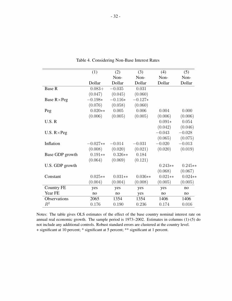
- 32 -

Table 4. Considering Non-Base Interest Rates

(1) (2) (3) (4) (5)Non- Non- Non- Non-

Dollar Dollar Dollar Dollar DollarBase R 0.083+ −0.035 0.031

(0.047) (0.045) (0.060)Base R×Peg −0.198∗ −0.116∗ −0.127∗

(0.076) (0.058) (0.060)Peg 0.020∗∗ 0.005 0.006 0.004 0.000

(0.006) (0.005) (0.005) (0.006) (0.006)U.S. R 0.091∗ 0.054

(0.042) (0.046)U.S. R×Peg −0.043 −0.028

(0.065) (0.075)Inflation −0.027∗∗ −0.014 −0.031 −0.020 −0.013

(0.008) (0.020) (0.021) (0.020) (0.019)Base GDP growth 0.191∗∗ 0.326∗∗ 0.184

(0.064) (0.069) (0.121)U.S. GDP growth 0.243∗∗ 0.245∗∗

(0.068) (0.067)Constant 0.025∗∗ 0.031∗∗ 0.036∗∗ 0.021∗∗ 0.024∗∗

(0.004) (0.004) (0.008) (0.005) (0.005)Country FE yes yes yes yes noYear FE no no yes no noObservations 2065 1354 1354 1406 1406R2 0.176 0.190 0.236 0.174 0.016

Notes: The table gives OLS estimates of the effect of the base country nominal interest rate onannual real economic growth. The sample period is 1973–2002. Estimates in columns (1)-(5) donot include any additional controls. Robust standard errors are clustered at the country level.+ significant at 10 percent; * significant at 5 percent; ** significant at 1 percent.

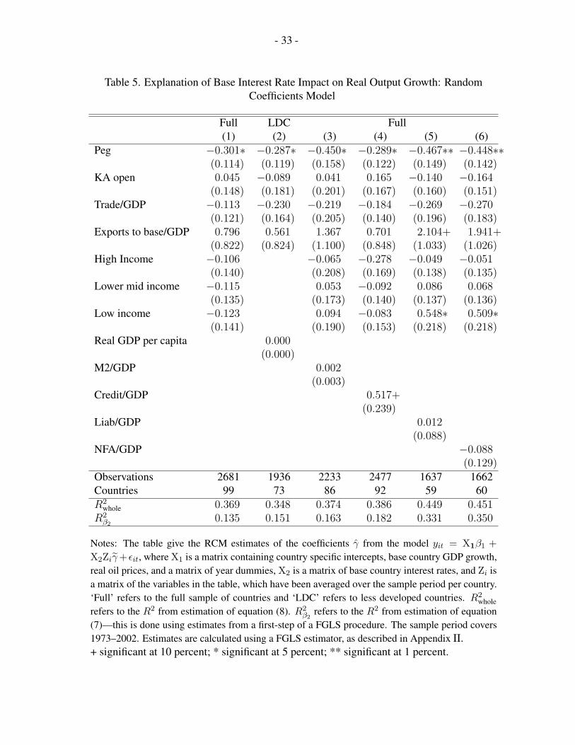
- 33 -

Table 5. Explanation of Base Interest Rate Impact on Real Output Growth: RandomCoefficients Model

Full LDC Full(1) (2) (3) (4) (5) (6)

Peg −0.301∗ −0.287∗ −0.450∗ −0.289∗ −0.467∗∗ −0.448∗∗(0.114) (0.119) (0.158) (0.122) (0.149) (0.142)

KA open 0.045 −0.089 0.041 0.165 −0.140 −0.164(0.148) (0.181) (0.201) (0.167) (0.160) (0.151)

Trade/GDP −0.113 −0.230 −0.219 −0.184 −0.269 −0.270(0.121) (0.164) (0.205) (0.140) (0.196) (0.183)

Exports to base/GDP 0.796 0.561 1.367 0.701 2.104+ 1.941+(0.822) (0.824) (1.100) (0.848) (1.033) (1.026)

High Income −0.106 −0.065 −0.278 −0.049 −0.051(0.140) (0.208) (0.169) (0.138) (0.135)

Lower mid income −0.115 0.053 −0.092 0.086 0.068(0.135) (0.173) (0.140) (0.137) (0.136)

Low income −0.123 0.094 −0.083 0.548∗ 0.509∗(0.141) (0.190) (0.153) (0.218) (0.218)

Real GDP per capita 0.000(0.000)

M2/GDP 0.002(0.003)

Credit/GDP 0.517+(0.239)

Liab/GDP 0.012(0.088)

NFA/GDP −0.088(0.129)

Observations 2681 1936 2233 2477 1637 1662Countries 99 73 86 92 59 60R2

whole 0.369 0.348 0.374 0.386 0.449 0.451R2

β20.135 0.151 0.163 0.182 0.331 0.350

Notes: The table give the RCM estimates of the coefficients γ from the model yit = X1β1 +X2Ziγ + εit, where X1 is a matrix containing country specific intercepts, base country GDP growth,real oil prices, and a matrix of year dummies, X2 is a matrix of base country interest rates, and Zi isa matrix of the variables in the table, which have been averaged over the sample period per country.‘Full’ refers to the full sample of countries and ‘LDC’ refers to less developed countries. R2

wholerefers to the R2 from estimation of equation (8). R2

β2refers to the R2 from estimation of equation

(7)—this is done using estimates from a first-step of a FGLS procedure. The sample period covers1973–2002. Estimates are calculated using a FGLS estimator, as described in Appendix II.+ significant at 10 percent; * significant at 5 percent; ** significant at 1 percent.

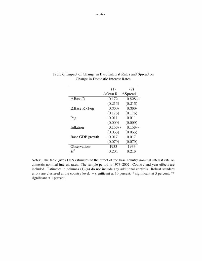
- 34 -

Table 6. Impact of Change in Base Interest Rates and Spread onChange in Domestic Interest Rates

(1) (2)∆Own R ∆Spread

∆Base R 0.172 −0.828∗∗(0.216) (0.216)

∆Base R×Peg 0.360∗ 0.360∗(0.176) (0.176)

Peg −0.011 −0.011(0.009) (0.009)

Inflation 0.156∗∗ 0.156∗∗(0.055) (0.055)

Base GDP growth −0.017 −0.017(0.079) (0.079)

Observations 1933 1933R2 0.204 0.216

Notes: The table gives OLS estimates of the effect of the base country nominal interest rate ondomestic nominal interest rates. The sample period is 1973–2002. Country and year effects areincluded. Estimates in columns (1)-(4) do not include any additional controls. Robust standarderrors are clustered at the country level. + significant at 10 percent; * significant at 5 percent; **significant at 1 percent.

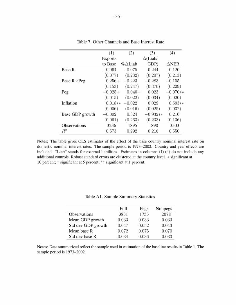
- 35 -

Table 7. Other Channels and Base Interest Rate

(1) (2) (3) (4)Exports ∆(Liab/to Base %∆Liab GDP) ∆NER

Base R −0.064 −0.075 0.244 −0.120(0.077) (0.232) (0.207) (0.213)

Base R×Peg 0.256+ −0.223 −0.283 −0.105(0.153) (0.247) (0.370) (0.229)

Peg −0.025+ 0.040+ 0.023 −0.070∗∗(0.015) (0.022) (0.034) (0.020)

Inflation 0.018∗∗ −0.022 0.029 0.593∗∗(0.006) (0.016) (0.025) (0.032)

Base GDP growth −0.002 0.324 −0.932∗∗ 0.216(0.061) (0.263) (0.233) (0.136)

Observations 3236 1895 1890 3503R2 0.573 0.292 0.216 0.550

Notes: The table gives OLS estimates of the effect of the base country nominal interest rate ondomestic nominal interest rates. The sample period is 1973–2002. Country and year effects areincluded. “Liab” stands for external liabilities. Estimates in columns (1)-(4) do not include anyadditional controls. Robust standard errors are clustered at the country level. + significant at10 percent; * significant at 5 percent; ** significant at 1 percent.

Table A1. Sample Summary Statistics

Full Pegs NonpegsObservations 3831 1753 2078Mean GDP growth 0.033 0.033 0.033Std dev GDP growth 0.047 0.052 0.043Mean base R 0.072 0.075 0.070Std dev base R 0.034 0.036 0.033

Notes: Data summarized reflect the sample used in estimation of the baseline results in Table 1. Thesample period is 1973–2002.

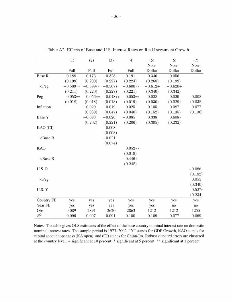
- 36 -

Table A2. Effects of Base and U.S. Interest Rates on Real Investment Growth

(1) (2) (3) (4) (5) (6) (7)Non- Non- Non-

Full Full Full Full Dollar Dollar DollarBase R −0.188 −0.173 −0.328 −0.191 0.346 −0.056

(0.198) (0.200) (0.227) (0.224) (0.268) (0.199)×Peg −0.589∗∗ −0.599∗∗ −0.567∗ −0.600∗∗ −0.612+ −0.620+

(0.211) (0.220) (0.227) (0.221) (0.340) (0.342)Peg 0.053∗∗ 0.056∗∗ 0.048∗∗ 0.053∗∗ 0.028 0.029 −0.008

(0.018) (0.018) (0.018) (0.019) (0.030) (0.029) (0.038)Inflation −0.029 −0.019 −0.025 0.105 0.087 0.077

(0.039) (0.047) (0.040) (0.152) (0.135) (0.136)Base Y −0.093 −0.026 −0.085 0.338 0.608∗

(0.202) (0.221) (0.206) (0.305) (0.232)KAO (CI) 0.008

(0.008)×Base R −0.021

(0.074)KAO 0.052∗∗

(0.019)×Base R −0.446+

(0.248)U.S. R −0.086

(0.182)×Peg 0.055

(0.340)U.S. Y 0.527∗

(0.234)Country FE yes yes yes yes yes yes yesYear FE yes yes yes yes yes no noObs. 3089 2891 2620 2863 1212 1212 1255R2 0.096 0.097 0.091 0.100 0.109 0.077 0.069

Notes: The table gives OLS estimates of the effect of the base country nominal interest rate on domesticnominal interest rates. The sample period is 1973–2002. “Y” stands for GDP Growth, KAO stands forcapital account openness (KA open), and (CI) stands for Chinn-Ito. Robust standard errors are clusteredat the country level. + significant at 10 percent; * significant at 5 percent; ** significant at 1 percent.

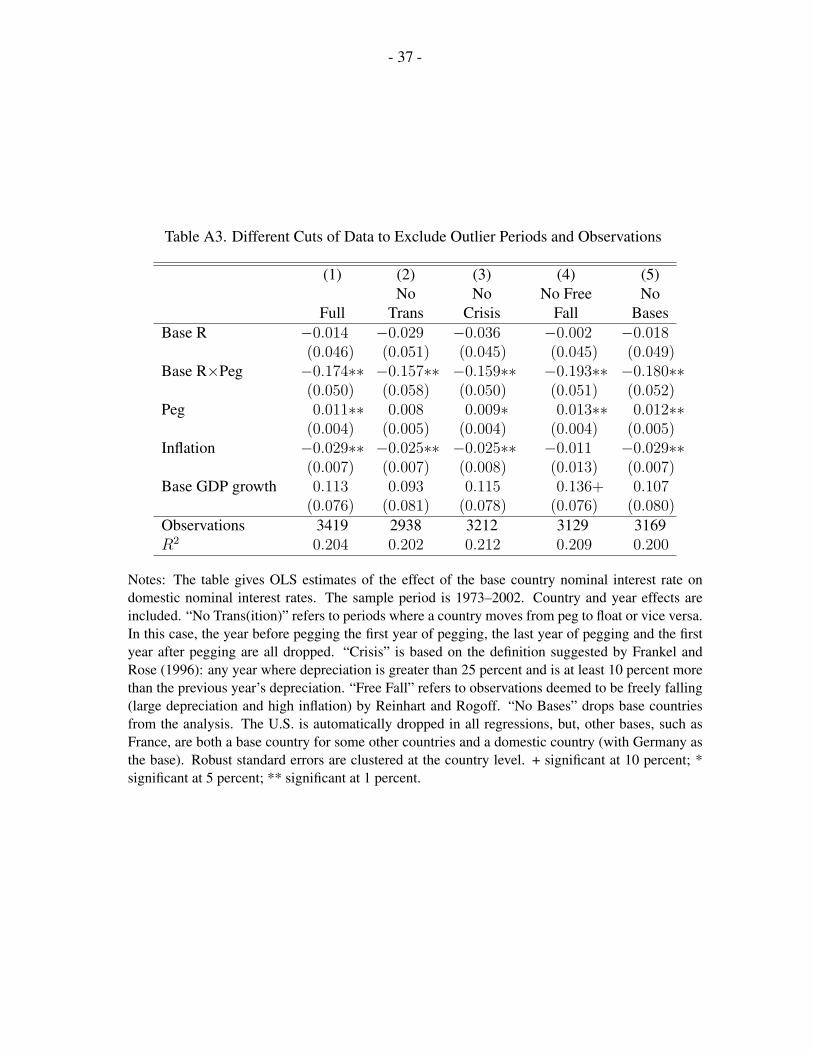
- 37 -

Table A3. Different Cuts of Data to Exclude Outlier Periods and Observations

(1) (2) (3) (4) (5)No No No Free No

Full Trans Crisis Fall BasesBase R −0.014 −0.029 −0.036 −0.002 −0.018

(0.046) (0.051) (0.045) (0.045) (0.049)Base R×Peg −0.174∗∗ −0.157∗∗ −0.159∗∗ −0.193∗∗ −0.180∗∗

(0.050) (0.058) (0.050) (0.051) (0.052)Peg 0.011∗∗ 0.008 0.009∗ 0.013∗∗ 0.012∗∗

(0.004) (0.005) (0.004) (0.004) (0.005)Inflation −0.029∗∗ −0.025∗∗ −0.025∗∗ −0.011 −0.029∗∗

(0.007) (0.007) (0.008) (0.013) (0.007)Base GDP growth 0.113 0.093 0.115 0.136+ 0.107

(0.076) (0.081) (0.078) (0.076) (0.080)Observations 3419 2938 3212 3129 3169R2 0.204 0.202 0.212 0.209 0.200

Notes: The table gives OLS estimates of the effect of the base country nominal interest rate ondomestic nominal interest rates. The sample period is 1973–2002. Country and year effects areincluded. “No Trans(ition)” refers to periods where a country moves from peg to float or vice versa.In this case, the year before pegging the first year of pegging, the last year of pegging and the firstyear after pegging are all dropped. “Crisis” is based on the definition suggested by Frankel andRose (1996): any year where depreciation is greater than 25 percent and is at least 10 percent morethan the previous year’s depreciation. “Free Fall” refers to observations deemed to be freely falling(large depreciation and high inflation) by Reinhart and Rogoff. “No Bases” drops base countriesfrom the analysis. The U.S. is automatically dropped in all regressions, but, other bases, such asFrance, are both a base country for some other countries and a domestic country (with Germany asthe base). Robust standard errors are clustered at the country level. + significant at 10 percent; *significant at 5 percent; ** significant at 1 percent.

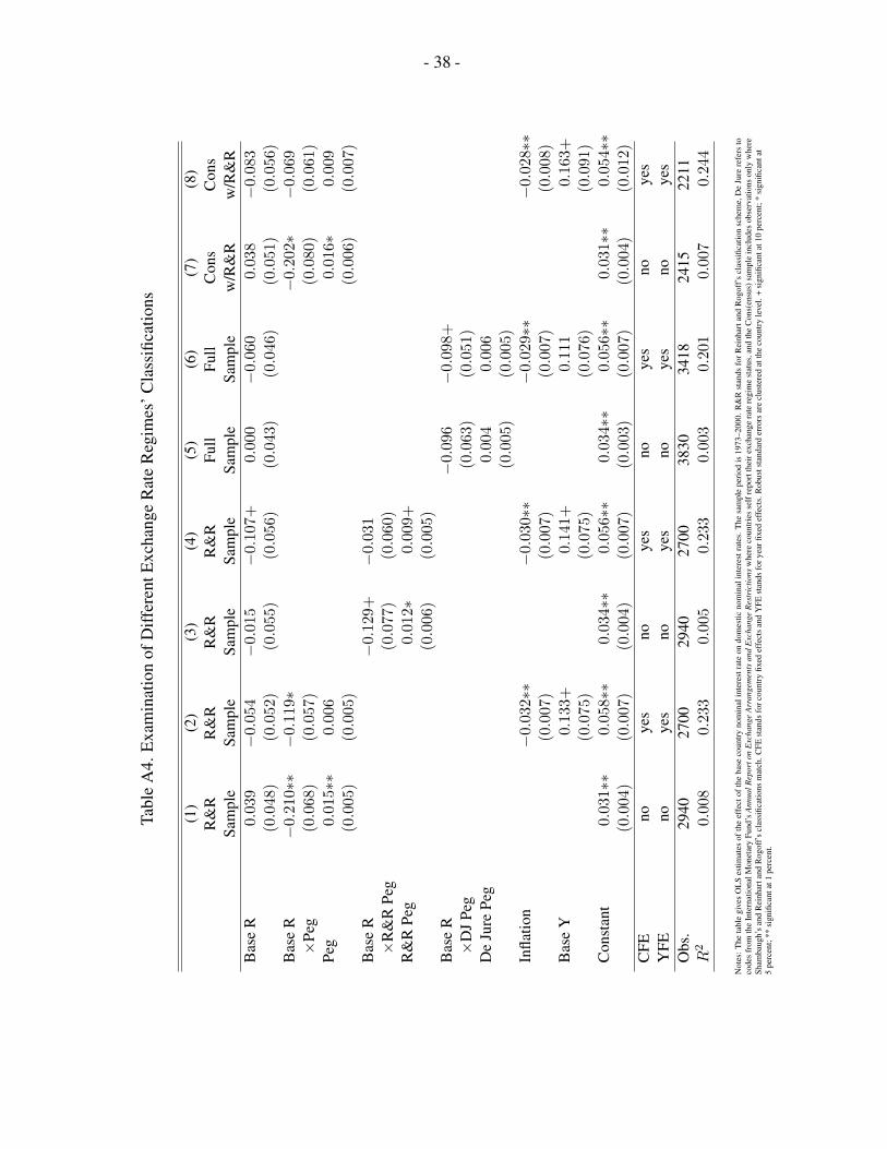
- 38 -

Tabl

eA

4.E

xam

inat

ion

ofD

iffer

entE

xcha

nge

Rat

eR

egim

es’C

lass

ifica

tions

(1)

(2)

(3)

(4)

(5)

(6)

(7)

(8)

R&

RR

&R

R&

RR

&R

Full

Full

Con

sC

ons

Sam

ple

Sam

ple

Sam

ple

Sam

ple

Sam

ple

Sam

ple

w/R

&R

w/R

&R

Bas

eR

0.03

9−0

.054

−0.0

15−0

.107

+0.

000

−0.0

600.

038

−0.0

83(0

.048

)(0

.052

)(0

.055

)(0

.056

)(0

.043

)(0

.046

)(0

.051

)(0

.056

)B

ase

R−0

.210∗∗

−0.1

19∗

−0.2

02∗

−0.0

69×P

eg(0

.068

)(0

.057

)(0

.080

)(0

.061

)Pe

g0.

015∗∗

0.00

60.

016∗

0.00

9(0

.005

)(0

.005

)(0

.006

)(0

.007

)B

ase

R−0

.129

+−0

.031

×R&

RPe

g(0

.077

)(0

.060

)R

&R

Peg

0.01

2∗0.

009+

(0.0

06)

(0.0

05)

Bas

eR

−0.0

96−0

.098

+×D

JPe

g(0

.063

)(0

.051

)D

eJu

rePe

g0.

004

0.00

6(0

.005

)(0

.005

)In

flatio

n−0

.032∗∗

−0.0

30∗∗

−0.0

29∗∗

−0.0

28∗∗

(0.0

07)

(0.0

07)

(0.0

07)

(0.0

08)

Bas

eY

0.13

3+0.

141+

0.11

10.

163+

(0.0

75)

(0.0

75)

(0.0

76)

(0.0

91)

Con

stan

t0.

031∗∗

0.05

8∗∗

0.03

4∗∗

0.05

6∗∗

0.03

4∗∗

0.05

6∗∗

0.03

1∗∗

0.05

4∗∗

(0.0

04)

(0.0

07)

(0.0

04)

(0.0

07)

(0.0

03)

(0.0

07)

(0.0

04)

(0.0

12)

CFE

noye

sno

yes

noye

sno

yes

YFE

noye

sno

yes

noye

sno

yes

Obs

.29

4027

0029

4027

0038

3034

1824

1522

11R

20.

008

0.23

30.

005

0.23

30.

003

0.20

10.

007

0.24

4

Not

es:

The

tabl

egi

ves

OL

Ses

timat

esof

the

effe

ctof

the

base

coun

try

nom

inal

inte

rest

rate

ondo

mes

ticno

min

alin

tere

stra

tes.

The

sam

ple

peri

odis

1973

–200

0.R

&R

stan

dsfo

rRei

nhar

tand

Rog

off’

scl

assi

ficat

ion

sche

me,

De

Jure

refe

rsto

code

sfr

omth

eIn

tern

atio

nalM

onet

ary

Fund

’sA

nnua

lRep

orto

nE

xcha

nge

Arr

ange

men

tsan

dE

xcha

nge

Res

tric

tions

whe

reco

untr

ies

self

repo

rtth

eire

xcha

nge

rate

regi

me

stat

us,a

ndth

eC

ons(

ensu

s)sa

mpl

ein

clud

esob

serv

atio

nson

lyw

here

Sham

baug

h’s

and

Rei

nhar

tand

Rog

off’

scl

assi

ficat

ions

mat

ch.C

FEst

ands

forc

ount

ryfix

edef

fect

san

dY

FEst

ands

fory

earfi

xed

effe

cts.

Rob

usts

tand

ard

erro

rsar

ecl

uste

red

atth

eco

untr

yle

vel.

+si

gnifi

cant

at10

perc

ent;

*si

gnifi

cant

at5

perc

ent;

**si

gnifi

cant

at1

perc

ent.

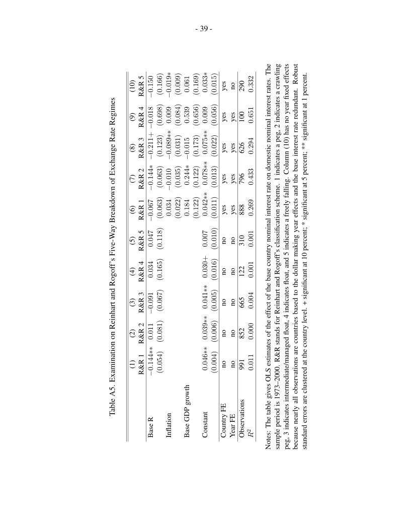
- 39 -

Tabl

eA

5.E

xam

inat

ion

onR

einh

arta

ndR

ogof

f’s

Five

-Way

Bre

akdo

wn

ofE

xcha

nge

Rat

eR

egim

es

(1)

(2)

(3)

(4)

(5)

(6)

(7)

(8)

(9)

(10)

R&

R1

R&

R2

R&

R3

R&

R4

R&

R5

R&

R1

R&

R2

R&

R3

R&

R4

R&

R5

Bas

eR

−0.1

44∗∗

0.01

1−0

.091

0.03

40.

047

−0.0

67−0

.144∗−0

.211

+−0

.018

−0.1

50(0

.054

)(0

.081

)(0

.067

)(0

.165

)(0

.118

)(0

.063

)(0

.063

)(0

.123

)(0

.698

)(0

.166

)In

flatio

n0.

034

−0.0

10−0

.089∗∗

0.00

9−0

.019∗

(0.0

22)

(0.0

35)

(0.0

31)

(0.0

84)

(0.0

09)

Bas

eG

DP

grow

th0.

184

0.24

4∗−0

.015

0.53

90.

061

(0.1

22)

(0.1

22)

(0.1

73)

(0.6

56)

(0.1

69)

Con

stan

t0.

046∗∗

0.03

9∗∗

0.04

1∗∗

0.03

0+0.

007

0.04

2∗∗

0.07

8∗∗

0.07

5∗∗

0.00

90.

033∗

(0.0

04)

(0.0

06)

(0.0

05)

(0.0

16)

(0.0

10)

(0.0

11)

(0.0

13)

(0.0

22)

(0.0

56)

(0.0

15)

Cou

ntry

FEno

nono

nono

yes

yes

yes

yes

yes

Yea

rFE

nono

nono

noye

sye

sye

sye

sno

Obs

erva

tions

991

852

665

122

310

888

796

626

100

290

R2

0.01

10.

000

0.00

40.

001

0.00

10.

269

0.43

30.

294

0.65

10.

332

Not

es:

The

tabl

egi

ves

OL

Ses

timat

esof

the

effe

ctof

the

base

coun

try

nom

inal

inte

rest

rate

ondo

mes

ticno

min

alin

tere

stra

tes.

The

sam

ple

peri

odis

1973

–200

0.R

&R

stan

dsfo

rRei

nhar

tand

Rog

off’

scl

assi

ficat

ion

sche

me.

1in

dica

tes

ape

g,2

indi

cate

sa

craw

ling

peg,

3in

dica

tes

inte

rmed

iate

/man

aged

float

,4in

dica

tes

float

,and

5in

dica

tes

afr

eely

falli

ng.C

olum

n(1

0)ha

sno

year

fixed

effe

cts

beca

use

near

lyal

lobs

erva

tions

are

coun

trie

sba

sed

toth

edo

llar

mak

ing

year

effe

cts

and

the

base

inte

rest

rate

redu

ndan

t.R

obus

tst

anda

rder

rors

are

clus

tere

dat

the

coun

try

leve

l.+

sign

ifica

ntat

10pe

rcen

t;*

sign

ifica

ntat

5pe

rcen

t;**

sign

ifica

ntat

1pe

rcen

t.

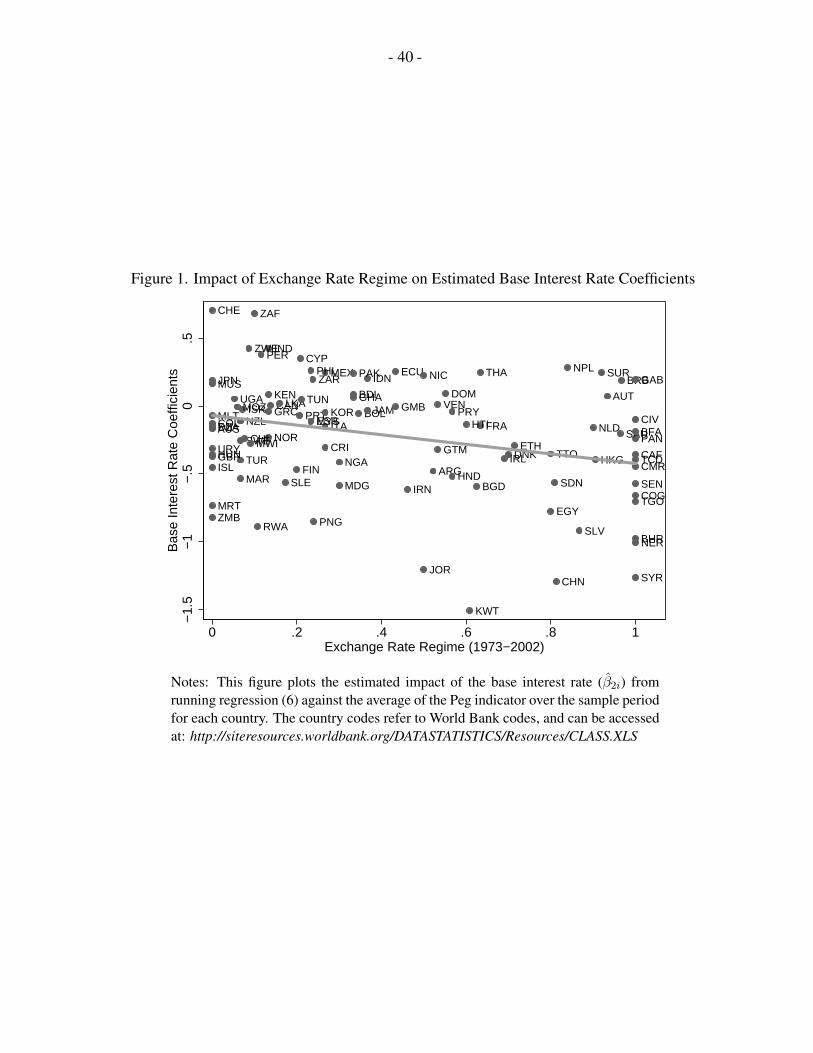
- 40 -

Figure 1. Impact of Exchange Rate Regime on Estimated Base Interest Rate Coefficients

GBR

AUT

DNK

FRAITA NLDNORSWE

CHE

CAN

JPN

FIN

GRC

ISLIRL

MLT PRTESP

TUR

AUSNZL

ZAF

ARG

BOL

CHLCOL

CRI

DOM

ECU

SLV

GTM

HTI

HND

MEX NIC

PAN

PRY

PER

URY

VEN

BRB

JAM

SUR

TTO

BHR

CYP

IRN

ISR

JOR

KWT

SAU

SYR

EGY

BGD

LKA

HKG

IND

IDN

KORMYS

NPLPAKPHL THA

DZA

BDI

CMRCAFTCD

COG

ZAR

ETH

GAB

GMBGHA

CIV

KEN

MDG

MWI

MRT

MUS

MAR

MOZ

NER

NGA

ZWE

RWA

SENSLE SDN

TGO

TUNUGA

BFA

ZMB

FJI

PNG

CHN

HUN

−1.

5−

1−

.50

.5B

ase

Inte

rest

Rat

e C

oeffi

cien

ts

0 .2 .4 .6 .8 1Exchange Rate Regime (1973−2002)

Notes: This figure plots the estimated impact of the base interest rate (β2i) fromrunning regression (6) against the average of the Peg indicator over the sample periodfor each country. The country codes refer to World Bank codes, and can be accessedat: http://siteresources.worldbank.org/DATASTATISTICS/Resources/CLASS.XLS

- 41 -

REFERENCES

Aghion, Philippe, Philippe Bacchetta, Romain Ranciere, and Kenneth S. Rogoff, 2005,“Productivity Growth and The Exchange Rate Regime: The Role of FinancialDevelopment” (unpublished; Cambridge, Mass.: Harvard University; Geneva: StudyCenter Gerzensee; Washington: International Monetary Fund).

Amemiya, Takeshi, 1978, “A Note on a Random Coefficients Model,” International EconomicReview, Vol. 19 (October), pp. 793–96.

Beck, Thorsten, Aslı Demirguc-Kunt, and Ross Levine, 1999, “A New Database on FinancialDevelopment and Structure.” World Bank Policy Research Working Paper No. 2146(Washington: World Bank).

Bernanke, Ben S., and Alan S. Blinder, 1992, “The Federal Funds Rate and the Channels ofMonetary Transmission,” American Economic Review, Vol. 82 (September) pp. 901–21.

Bernanke, Ben S., Mark Gertler, and Mark Watson, 1997, “Systematic Monetary Policy andthe Effects of Oil Price Shocks,” Brookings Papers on Economic Activity, No. 1,pp. 91–142.

Bernanke, Ben S., and Ilian Mihov, 1998, “The Liquidity Effect and Long-Run Neutrality,”Carnegie Rochester Conference Series on Public Policy, Vol. 49 (December),pp. 149–94.

Bertrand, Marianne, Esther Duflo, and Sendhil Mullainathan, 2004, “How Much Should WeTrust Differences-in-Differences Estimates?” Quarterly Journal of Economics, Vol. 119,(February), pp. 249-75.

Borensztein, Eduardo, Jeromin Zettelmeyer, and Thomas Philippon, 2001, “MonetaryIndependence in Emerging Markets: Does the Exchange Rate Regime Make aDifference?” (January). IMF Working Paper No. 01/1 (Washington: InternationalMonetary Fund).

Broda, Christian, 2004, “Terms of Trade and Exchange Rate Regimes in DevelopingCountries,” Journal of International Economics, Vol. 63, pp. 31–58.

Calvo, Guillermo A., Leonardo Leiderman, and Carmen M. Reinhart, 1993, “Capital Inflowsand Real Exchange Rate Appreciation in Latin America: The Role of External Factors,”IMF Staff Papers, Vol. 40 (March), pp. 108–51.

———, 1996, “Inflows of Capital to Developing Countries in the 1990s,” Journal ofEconomic Perspectives, Vol. 10 (Spring), pp. 123–39.

Canova, Fabio, 2005, “The Transmission of US Shocks to Latin America,” Journal of AppliedEconometrics, Vol. 20 (March), pp. 229–51.

- 42 -

Chinn, Menzie D., and Hiro Ito, 2005, “What Matters for Financial Development? CapitalControls, Institutions, and Interactions” (unpublished; Madison: University ofWisconsin; Portland: Portland State University. Revised version of NBER WorkingPaper No. 8967, May 2002).

Christiano, Lawrence J., Martin Eichenbaum, and Charles L. Evans, “Monetary PolicyShocks: What Have We Learned and to What End?” 1999, in John B. Taylor andMicheal Woodford, eds., Handbook of Macroeconomics, Vol. 1A (New York:North-Holland, Elsevier), chapter 2, pp. 65–148.

Clarida, Richard, Jordi Galı, and Mark Gertler, 2000, “Monetary Policy Rules andMacroeconomic Stability: Evidence and Some Theory,” Quarterly Journal ofEconomics, Vol. 115 (February), pp. 147–80.

di Giovanni, Julian, Justin McCrary, and Till von Wachter, 2005, “Following the Leader:Simple Estimates of the Effect of Monetary Policy on the Economy” (May). IMFWorking Paper No. 05/86 (Washington: International Monetary Fund).

Dornbusch, Rudiger, 1985, “Policy and Performance Links Between LDC Debtors andIndustrial Nations,” Brookings Papers on Economic Activity, No. 2, pp. 303–68.

Flood, Robert P., and Andrew K. Rose, 1995, “Fixing Exchange Rates: A Virtual Quest forFundamentals,” Journal of Monetary Economics, Vol. 36, pp. 3–37.

———, 1999, “Understanding Exchange Rate Volatility Without the Contrivance ofMacroeconomics,” Economic Journal, Vol. 109 (November), pp. F660–72.

Frankel, Jeffrey A., and Andrew K. Rose, 1996, “Currency Crashes in Emerging Markets: AnEmpirical Treatment,” Journal of International Economics, Vol. 41 (November),pp. 351–66.

Frankel, Jeffrey A., and Nouriel Roubini, 2001, “The Role of Industrial Country Policies inEmerging Market Crises” (December). NBER Working Paper No. 8634 (Cambridge,Mass.: National Bureau of Economic Research).

, Sergio L. Schmukler, and Luis Serven, 2004, “Global Transmission of Interest Rates:Monetary Independence and Currency Regimes,” Journal of International Money andFinance, Vol. 23 (September), pp. 701–34.

Froot, Kenneth A., and Richard H. Thaler, 1990, “Anomalies: Foreign Exchange,” Journal ofEconomics Perspectives, Vol. 4 (Summer), pp. 179–92.

Hamilton, James D., and Ana Maria Herrera, 2004, “Oil Shocks and AggregateMacroeconomic Behavior: The Role of Monetary Policy,” Journal of Money, Credit, andBanking, Vol. 36 (April), pp. 265–86.

- 43 -

Hausmann, Ricardo, Michael Gavin, Carmen Pages-Serra, and Enernesto Stein, 1999,“Financial Turmoil and the Choice of the Exchange Rate Regime.” IADB WorkingPaper No. 400 (Washington: Inter-American Development Bank).

Hsiao, Cheng, 2003, Analysis of Panel Data, 2 ed. (Cambridge, UK: Cambridge UniversityPress).

———, and M. Hashem Pesaran, 2004, “Random Coefficient Panel Data Models”(unpublished; Los Angeles: University of Southern California; Cambridge: Universityof Cambridge).

Husain, Aasim M., Ashoka Mody, and Kenneth S. Rogoff, 2005, “Exchange Rate RegimeDurability and Performance in Developing Versus Advanced Economies,” Journal ofMonetary Economics, Vol. 52 (January), pp. 35–64.

International Monetary Fund (IMF), Annual Report on Exchange Arrangements and ExchangeRestrictions (Washington, D.C.: International Monetary Fund). Various Issues.

Kim, Soyoung, 2001, “International Transmission of U.S. Monetary Policy Shocks: Evidencefrom VAR’s,” Journal of Monetary Economics, Vol. 48, pp. 339–72.

Lane, Philip R., and Gian Maria Milesi-Ferretti, 2001, “The External Wealth of Nations:Measures of Foreign Assets and Liabilities for Industrial and Developing Countries,”Journal of International Economics, Vol. 55 (December), pp. 263–94.

Mackowiak, Bartosz, 2003, “External Shocks, U.S. Monetary Policy and MacroeconomicFluctuations in Emerging Markets” (unpublished; Berlin: Humoldt University ofBerlin).

Miniane, Jacques, and John H. Rogers, 2003, “Capital Controls and the InternationalTransmission of U.S. Money Shocks” (September). International Finance DiscussionPaper No. 778 (Washington: Boards of Governors of the Federal Reserve System).

Neumeyer, Pablo A., and Fabrizio Perri, 2005, “Business Cycles in Emerging Economies:The Role of Interest Rates.” Forthcoming, Journal of Monetary Economics.

Obstfeld, Maurice, Jay C. Shambaugh, and Alan M. Taylor, 2004, “Monetary Sovereignty,Exchange Rates, and Capital Controls: The Trilemma in the Interwar period,” IMF StaffPapers, Vol. 51 (Special Issue), pp. 75–108.

———, 2005, “The Trilemma in History: Tradeoffs among Exchange Rates, MonetaryPolicies, and Capital Mobility,” Review of Economics and Statistics, Vol. 87 (August),pp. 423–38.

Pesaran, M. Hashem, 2004, “General Diagonist Tests for Cross Section Dependence inPanels” (unpublished; Cambridge: University of Cambridge).

- 44 -

Reinhart, Carmen M., and Vincent Raymond Reinhart, 2001, “What Hurts Most? G-3Exchange Rate or Interest Rate Volatility” (October). NBER Working Paper No. 8535(Cambridge, Mass.: National Bureau of Economic Research).

Reinhart, Carmen M., and Kenneth S. Rogoff, 2004, “The Modern History of Exchange RateArrangements: A Reinterpretation,” Quarterly Journal of Economics, Vol. 119(February), pp. 1–48.

Romer, Christina D., and David H. Romer, “Does Monetary Policy Matter? A New Test in theSpirit of Friedman and Schwartz,” 1989, in Oliver J. Blanchard and Stanley Fischer, eds.,NBER Macroeconomics Annual 4, (Cambridge, Mass.: The MIT Press), pp. 121–170.

Rotemberg, Julio J., and Michael Woodford, “An Optimization-Based Econometric Model forthe Evaluation of Monetary Policy,” 1997, in Ben S. Bernanke and Julio Rotemberg,eds., NBER Macroeconomics Annual, Vol. 12 (Cambridge, Mass.: MIT Press),pp. 297–346.

Shambaugh, Jay C., 2004, “The Effects of Fixed Exchange Rates on Monetary Policy,”Quarterly Journal of Economics, Vol. 119, pp. 301-52.

Smith, Ron P. and Ana-Maria Fuertes, 2004, “Panel Time-Series” (unpublished; London:Birkbeck College, London; Sir John Cass Business School, City University).

Taylor, John B., 1993, “Discretion Versus Policy Rules in Practice,” Carnegie RochesterConference Series on Public Policy, Vol. 93 (December), pp. 195–214.

Uribe, Martın and Vivian Z. Yue, 2005, “Country Spreads and Emerging Countries: WhoDrives Whom?” Forthcoming, Journal of International Economics.