Embed Size (px)
Citation preview
Page| 1
THE IMPACT OF FREE TRADE AGREEMENT ON TRADE
FLOW OF GOODS IN VIETNAM1
NGUYEN TRONG HOAI
UNIVERSITY OF ECONOMICS HO CHI MINH CITY
NGUYEN QUANG HUY
VIETNAM-NETHERLANDS PROGRAMME
May 2015
ABSTRACT
This study analyzes the effect of free trade agreement (FTA) on merchandise
export of Vietnam by applying gravity model. The model is evaluated on a sample
of 185 countries in the period 1990-2012 using country level data for total
export value of goods. In order to deal with multilateral resistance terms in the
model, the study employs the fixed-effect model to control for unobservable
factors. Due to zero-export value in data set, the export-plus-one model, the
multiplicative form of gravity model and adjusted sample selection model (SSM)
are used to solve the zero-value in export between Vietnam and trading partners.
Previous research argues for the lack of exclusion restriction in using SSM
proposed by Heckman (1979), the paper proves that sample selection approach
is more efficient than the other two models. The results from the study find out
that Vietnam have positive relationship with the trade outflow. This finding is
supported by the previous papers testing the impact of AFTA on the trade flow.
Key words: Free Trade Agreement, gravity model, total bilateral trade, export
1 Contact: [email protected]
Page| 2
1 Introduction
According to World Trade Organization, Vietnam is now official member of
eight free trade agreements which are signed and into force; and, Vietnam is also
launching negotiation with a number of countries and economic groups to
establish other free trade agreements such as TPP, ASEAN-EU FTA. On the one
hand, free trade is espoused in improving the trade and welfare of signing
countries. This belief is developed from the absolute advantage by Adam Smith,
comparative advantage by David Ricardo, Heckscher-Ohlin model by Eli
Heckscher and Bertil Ohlin to Paul Krugman with economies of scale and product
differentiation. On the other hand, Michaely (1996) not only accepted the gain
from free trade but he also pointed out the loss if countries build trading blocs.
The “trade diversion” is the terminology for diverting trade from countries to
countries. Therefore, question should be asked is how trade flow of Vietnam is
affected by her free trade agreements.
Empirically, there are a vast number of papers investigating the
relationship between free trade agreement and bilateral trade. Hur, Alba &Park
(2009) conducted a research to evaluate the Hub-and-Spoke problem in free
trade agreements by using panel data analysis of 96 countries from 1960 to
2000; and concluded that in spite of the existing of overlapping free trade
agreement, export also increased. Other relevant paper by Baier & Berstrand
(2009), that gives comprehensive contribution to the empirical model to
investigate the effect of free trade agreement on international trade flow, also
found the similar positive linkage. However, Aitken (1972) did an empirical
research on trade creating and trade diverting after the establishment of EEC and
EFTA. He found that EEC increased trading value of member countries
significantly by trade creating and trade diverting, whereas the effect of EFTA is
not considerably because of trade diverting. Besides, Jugurnath et al (2007)
carried out a research on many free trade agreements. The authors asserted that
ASEAN FTA, CER increased its members’ trade significantly, while MERCOSUR,
NFTA and APEC created the trade diversion. Relating to Vietnam context, papers
Page| 3
analyze the linkage between free trade agreement and trade flow in Vietnam is
limited. For instance, Thai (2006) used gravity model to calculate the trade
between Vietnam and twenty-three European countries. The paper found the
determinants in trading such as economic characteristics, exchange rate volatility
and the demand of destination. However, free trade agreement is not mentioned
in the paper because Vietnam and those countries have not signed FTA yet. Other
paper investigates the impact of ASEAN Free Trade Agreement (AFTA) on
Vietnam’s economy is by Fukase & Martin (2001). The authors concluded that
impact of AFTA is not significant. Agricultural sector gets benefit from that free
trade because of exporting opportunity to ASEAN market, while some other
industries is hurt and need to be protected due to ASEAN competitors. Therefore,
this study will analyze the role of free trade agreement on trade flow of goods in
Vietnam by applying gravity model for panel of 184 countries over the period
1990-2012. The study is carried out by using Fixed Effect model proposed by
Baier & Bergstrand (2007), Sample Selection model (SSM) by Helpman et al
(2008), and Poisson Pseudo Maximum Likelihood model by Tenreyro & Silva
(2008).
2 Free trade agreement
After establishing trading bloc, member countries can shift import from
higher-taxed suppliers to lower-no taxed suppliers; and, domestic goods are
substituted by foreign low-cost goods. Johnson (1974) stated these above
movements will balance the increasing-welfare. Lipsey (1957) and Bhagwati
(1971) defined the trade diversion as the change in the locus of production from
initial lower supplier to higher member suppliers. Trade creation is defined as
the increase in trade between member countries. Johnson (1974) argued that
trade diversion can give a transfer from locus of production which negatively
impact on welfare, and create a substitution effect which positively impact on
welfare. Furthermore, Michaely (1976) asserted that trade liberalization impacts
on the trade pattern of signing countries in three ways. First effect is the increase
in new trade flow between bloc’s members. Secondly, reducing trade barrier can
Page| 4
divert the import from non-member suppliers to member suppliers. Finally, the
change in term of trade is an attributable to a rise in demand of substitute
commodity.
Chaney (2008) stated that the change in trade flow due to trade barrier
shock can be explained through two mechanisms. The first mechanism is the
intensive margin which is the increase in exporting volume of incumbent firms.
The second one is the extensive margin which is the change in the number of
exporter in different sectors. In general, trade barrier reduction such as free
trade agreement between two countries leads to the change in the number of
good each firm exports, and new exporters can enter the market. Crozet and
Koenig (2010) confirmed the theory in heterogeneous firms established in
Chaney (2008). The paper disintegrated effect of trade cost on trade flow in to
intensive margin and extensive margin as follow:
(2.1)
Where j
M
is the total trade cost elasticity of trading value
j
EXT
is the trade cost elasticity of external margins
j
INT
is the trade cost elasticity of internal margins
Crozet and Koenig (2010) concluded that the change in trade flow due to
fluctuation in trade cost varied across the industries. In details, the reducing in
trade barrier impacts on trade level greater in homogenous industries than more
heterogeneous industries. Extensive margin effect can dominate the intensive
margin effect in industry with high differentiated product. Moreover, Helpman,
Melitz, and Rubinstein (2007) stated that the profitability of firm export is higher
if the importing countries’ demand is higher, and lower trade costs. On the other
hand, firm will not export if the profit of firm is negative. That can explain the
zero value in export between two countries. He showed the primary bias in
estimating impact of trade barrier on trade flow is attributed to ignoring
j j j
M EXT INT
Page| 5
extensive margin effect. The reducing in trade friction may not only lead to the
expansion of trade between existent country pairs, but also to create new trading
partners.
3 Gravity model for free trade agreement
Aitken (1973) is the first author which applied the theory of gravity model in
order to estimate the effect of European Economic Community (EEC) and
European Free Trade Association (EFTA) on the import and export of member
countries. In his model, he proposed a number of indicators for conceptions in
the theoretical model. The dependent variable was export value. The
independent variables were Free trade agreement, Income of exporting
countries, Income of Importing countries, Distance between trading partners.
Those indicators have been used by latter researches on observing the impact of
FTA on trade flow of countries.
Trade flow
In empirical papers, there are three indicators for trade flow between
countries. Firstly, McCallum (1995) used the shipment value from one country to
other country as the representative for trade flow. In his paper, he analyzed the
impact of trade border effect in the trade between The United States of America
(USA) and Canada. The idea of research is that within-provincial trade of Canada
is greater than the trade with USA’s states. By applying the gravity model as
follow:
ij i j ij ij ijx a by cy ddist eDUMMY u
(2.2)
Where xij is the total export from region i to region j
Anderson and Wincoop (2003) examined the results obtaining from
McCallum (1995). The authors argued that the result is overestimated because it
omitted trade resistance variables which are called multilateral resistance terms
Page| 6
(MRTs). Anderson and Wincoop (2003) proposed a new estimated model as
follow:
(2.3)
The model also used the export from countries i to j as the dependent
variable for trade flow. The differences with McCallum (1995) are the
variables , the multilateral resistance terms. The meaning of MRTs is
that it indicated the average price of export country to the rest of the world’s
price. The definitions of MRTs are as follow:
(2.4)
(2.5)
Baier and Bergstrand (2007) did a research to estimate the impact of FTA
on trade flow. The paper used data of 96 countries around the world from 1960
to 2000. In his estimation model, the trade flow between i and j is the export
value from i to j divided by the GDP deflator to obtain real trade flow. Hur, Alba,
and Park (2010) applied the gravity model proposed by Baier and Bergstrand
(2007) to find out the hub-spoke effect of FTA using data on 96 countries around
the world throughout 40 years from 1960. In the model, dependent variable is
real exporting value, the nominal exporting value divided by GDP deflator.
However, Yang and Martinez-Zarzoso (2013) estimated whether ASEAN-China
Free Trade agreement is trade creation or trade diversion. In the paper, current
export level in US dollar represent for trade flow concept in international trade.
On the other hand, Jugurnath, Stewart, and Brook (2007) did not exploit
the export value as an indicator for trade flow. Instead of that, current import
value is use as a dependent variable in the model. The reason is that country
Page| 7
often strictly reports its import value for the tax purpose, so the import value is
more correct than export value.
Free Trade Agreement
The primary effect of FTA on trade flow is through the elimination of trade
tariffs, so many research papers has analyzed trade cost as a tool for evaluation
the impact of FTA. Anderson and Wincoop (2003) use the following
measurement:
p
ij ij ijt b d (2.6)
bij indicates the border effect in his analysis. The variable will take the value of 1
if two regions is in same country, otherwise, it is equal to one add trading tax.
Baier and Bergstrand (2007) estimated the impact of FTA on trade flow of
countries by using variable FTA as a dummy variable. The variable FTA took
value of 1 of exporter and importer are in the same free trade area, unless FTA
was equal to 0. The paper use panel data and fixed effect estimation to find the
FTA’s coefficient, and the result showed that there is positive relationship
between FTA and trade flow. Basing on Baier and Bergstrand (2007), Jugurnath,
Stewart, and Brooks (2007) also used FTA as dummy variable in their paper.
However, the paper not only estimated the impact of FTA on trade flow, but also
intent to find the trade diversion and trade creation effect of FTA. Therefore, they
set up more dummies variable to separate the diversion and creation effect in
trade. The model is as follow:
1 1 1
log ij ik kj ki kj
k k k
IMPORT aX RTA RTA RTA RTA
(2.7)
In the model, i is the importing country, j is exporter, and k indicates the
Regional Trade Agreement (RTA) k. Unlike in Baier and Bergstrand (2007), there
are separate RTAs for two countries to analyze the trade creation and trade
diversion of RTAs. The paper concluded that regional trade agreement of ASEAN,
CER are trade creation while APEC, MERCOSUR, and NAFTA have a tendency to
increase trade within regional member or may be trade diversion. Furthermore,
Page| 8
Yang and Martinez-Zarzoro (2013) estimated the relationship between ASEAN-
China (ACFTA) on trade flow of member countries. The model of paper set up
three types of FTA dummy variables. The first FTA variable is equal one if both
export and import countries are in same FTA. The second dummy FTA is equal 1
if exporter is in the ACFTA, and importer is not in ACFTA. The final dummy FTA is
equal 1 if only importer is in ACFTA. FTA dummy variable is applied to measure
free trade agreement effect in Hur, Alba, and Park (2010). Objectives of the paper
are to answer two questions. The first question is the effect of FTA on trade by
using dummy variable FTA as in Baier and Bergstrand (2007). The second
question is the hub and spoke nature of FTA.
In conclusion, indicator for Free Trade Agreement is the dummy variable
taking value of 1 if two countries is in same FTA, otherwise, FTA equal to 0. The
coefficient of FTA variable is expected to be positive
Income of exporting and importing countries
Aitken (1973) took the nominal GDP of exporting and importing countries
as measurement of income concept in international trade. This indicator for
income has been accepted by other empirical papers. Anderson and Wincoop
(2003) selected the gross domestic production as a proxy for income of trading
countries. The nominal gross domestic production was also used in paper of
Jugurnath, Stewart, and Brooks (2007). However, Baier and Bergstrand (2007)
divided nominal GDP by the GDP deflator in order to obtain real GDP. There was
no clear argument between choosing nominal GDP or real GDP as an indicator for
income. In all mentioned papers, both income of exporting country and
importing countries have been found to impact positively on the trade flow.
Distance
The development of information technology and transportation
infrastructure has leaded to a decrease in transport cost between countries, yet
the question arose is whether the distance effects on export of goods is important
or not. Disdier and Head (2008) analyzed the distance effect on trading between
Page| 9
two countries. The paper collected 1467 coefficients of distance on trade flow
from the estimation of 103 papers, and then found out that the change in the
value of distance elasticity of trade flow. The authors stated that the mean effect
of distance is approximate 0.9 meaning that 10 percent increase in the distance
of two countries; the trade value will decrease 9 percent.
Carrère and Schiff (2005) conducted a paper to answer for puzzle in
distance of trade. In the paper, the authors decomposed the components of
transport cost into non-distance trade cost whose costs do not related to distance
of goods export, and distance cost. By analyzing the transport cost of data from
150 countries between 1962 and 2000, Carrere and Schiff (2005) stated that the
decision on how much to trade to foreign countries locating at varied distance
depends on the combination of non-distance cost and distance cost. Although the
paper did not solve which costs can be dominance factors, the measurement
showed that the distance’s role in trade is rose throughout the period.)
Relating to measure distance variable in empirical study, Baier and
Bergstrand (2007) measured the distance variable by the distance between
economic center of countries, while Yang and Martinez-Zarzoso (2014) estimate
the distance variable by calculating the great circle distance from capital of
exporting countries to capital of importing countries. In both papers, the
expected impact of distance on trade flow is negative.
Exchange rate
The role of exchange rate in international trade is an ongoing argument
within empirical studies. Rose and Wincoop (2001) looked into the effect of
currency union on European countries on the trade flow. The paper used
Economic and Monetary Union (EMU) as an indicator for no exchange rate
volatility in international trade. In the paper, if the EMU impacts positively on the
trade flow of member countries, the exchange rate volatility has negative
relationship on export and import value. By using data on trade of 200 countries
from 1970 to 1995, the paper applied gravity model adding EMU dummies
Page| 10
variable for estimation. The result indicated that the trade between EMU
countries is higher than those without in EMU. Rose and Wincoop (2001) posed
the importance of currency barrier in trade flow. McKenzie (2002) conducted a
paper reviewing previous researches on the risk of exchange rate’s effect to
trade. The papers also found out the conclusion supporting Rose and Wincoop
(2001); the result is that exchange rate volatility impact negatively on
international trade, yet the degree of impact varying among the paper. Recently,
Al-Rashidi and Lahiri (2013) used heterogeneous firm-selection model to
estimate that relationship, and the result pointed out that exchange rate volatility
coefficient in model is statistically significant.
4 Methodology
The study will apply the gravity model considered the powerful one in
analyzing trade policies in order to estimate the coefficients between trade flow
and FTA (Anderson & vanWincoop, 2003; Baier & Bergstrand, 2007; Silva &
Tenreyro, 2006; Baier & Bergstrand, 2009; Zarzoso, 2013; Head & Mayer. 2013).
The functional form is as follow:
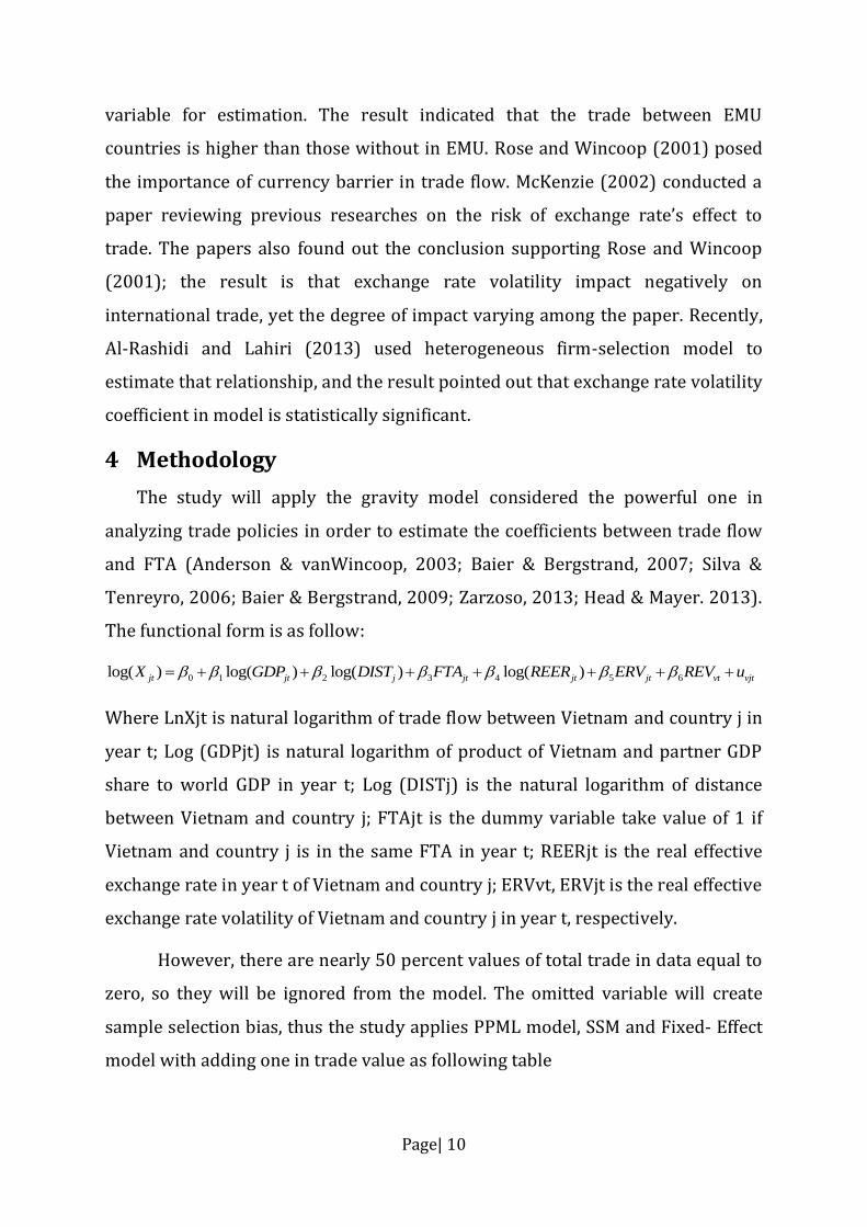
0 1 2 3 4 5 6log( ) log( ) log( ) log( )jt jt j jt jt jt vt vjtX GDP DIST FTA REER ERV REV u
Where LnXjt is natural logarithm of trade flow between Vietnam and country j in
year t; Log (GDPjt) is natural logarithm of product of Vietnam and partner GDP
share to world GDP in year t; Log (DISTj) is the natural logarithm of distance
between Vietnam and country j; FTAjt is the dummy variable take value of 1 if
Vietnam and country j is in the same FTA in year t; REERjt is the real effective
exchange rate in year t of Vietnam and country j; ERVvt, ERVjt is the real effective
exchange rate volatility of Vietnam and country j in year t, respectively.
However, there are nearly 50 percent values of total trade in data equal to
zero, so they will be ignored from the model. The omitted variable will create
sample selection bias, thus the study applies PPML model, SSM and Fixed- Effect
model with adding one in trade value as following table
Page| 11
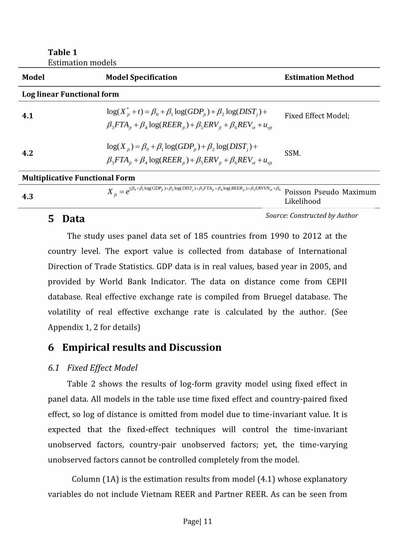
Table 1 Estimation models
5 Data
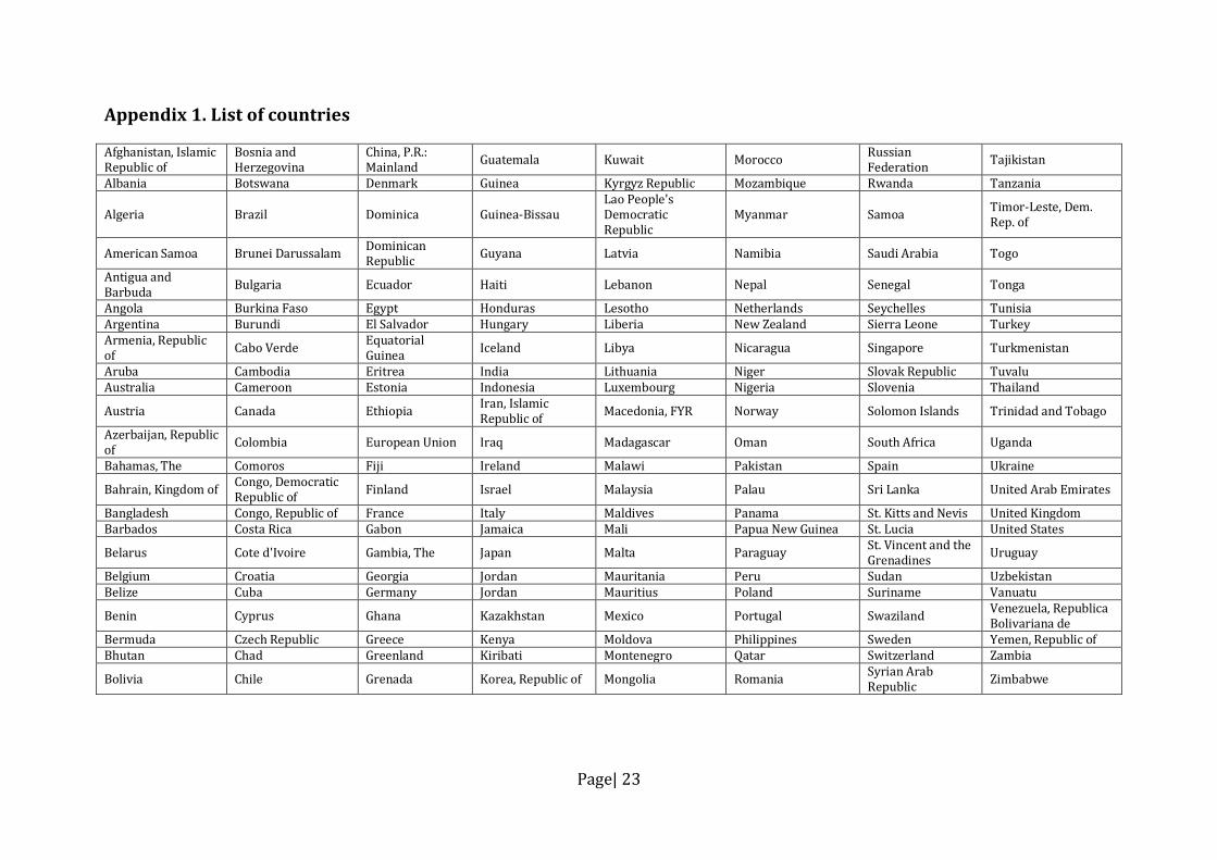
The study uses panel data set of 185 countries from 1990 to 2012 at the
country level. The export value is collected from database of International
Direction of Trade Statistics. GDP data is in real values, based year in 2005, and
provided by World Bank Indicator. The data on distance come from CEPII
database. Real effective exchange rate is compiled from Bruegel database. The
volatility of real effective exchange rate is calculated by the author. (See
Appendix 1, 2 for details)
6 Empirical results and Discussion
6.1 Fixed Effect Model
Table 2 shows the results of log-form gravity model using fixed effect in
panel data. All models in the table use time fixed effect and country-paired fixed
effect, so log of distance is omitted from model due to time-invariant value. It is
expected that the fixed-effect techniques will control the time-invariant
unobserved factors, country-pair unobserved factors; yet, the time-varying
unobserved factors cannot be controlled completely from the model.
Column (1A) is the estimation results from model (4.1) whose explanatory
variables do not include Vietnam REER and Partner REER. As can be seen from
Model Model Specification Estimation Method
Log linear Functional form
4.1 4.2
*
0 1 2
3 4 5 6
log( ) log( ) log( )
log( )
jt jt j
jt jt jt vt vjt
X t GDP DIST
FTA REER ERV REV u
0 1 2
3 4 5 6
log( ) log( ) log( )
log( )
jt jt j
jt jt jt vt vjt
X GDP DIST
FTA REER ERV REV u
Fixed Effect Model; SSM.
Multiplicative Functional Form
4.3 0 1 2 3 4 5 6( log( ) log( ) log( ) )jt j jt jt vt jt ijtGDP DIST FTA REER ERVVN ERVP u
jtX e
Poisson Pseudo Maximum Likelihood
Source: Constructed by Author
Page| 12
the result, three independent variables’ coefficients are statistical significance at
1% (Dummy variable for Asian Crisis, and Global Crisis) and FTA’s coefficient is
statistically significant at 10%; log of world share GDP’s coefficient does not have
statistical meaning while log of distance is omitted in FEM due to time-invariant
value. The variable of interest FTA’s coefficient is 1.367 which is consistent with
the expectation that FTA will increase the export between Vietnam and its
trading members. In details, on average, if Vietnam and trading partner is in the
FTA, the total export will be merely 3.9 times (e1.367) higher than the trade value
between Vietnam and non-FTA trading partner, other factors are the same.
Relating to column (2A), after adding exchange rate volatility variables, the
results do not change in term of coefficient’s sign; the differences are the variable
Log of World Share GDP is statistically-significant negative at 10%. FTA’s
coefficient is statistical significance at 1% in this column, and value is 3.517
which is higher than the one in column (1A), ceteris paribus. This indicates that if
two countries are in FTA, the export value is average 33.68 times higher export
value between Vietnam and non-FTA countries, ceteris paribus. The results from
FEM regressions with dependent variable are export plus one in Table 2 accepts
the hypothesis that FTA will increase the trade flow between Vietnam and FTA-
member trading countries. The coefficient in model (2A) is considerably higher
than FTA’s coefficient in model (1A); the results will be compared with
estimation result of SSM and PPML model.
Page| 13
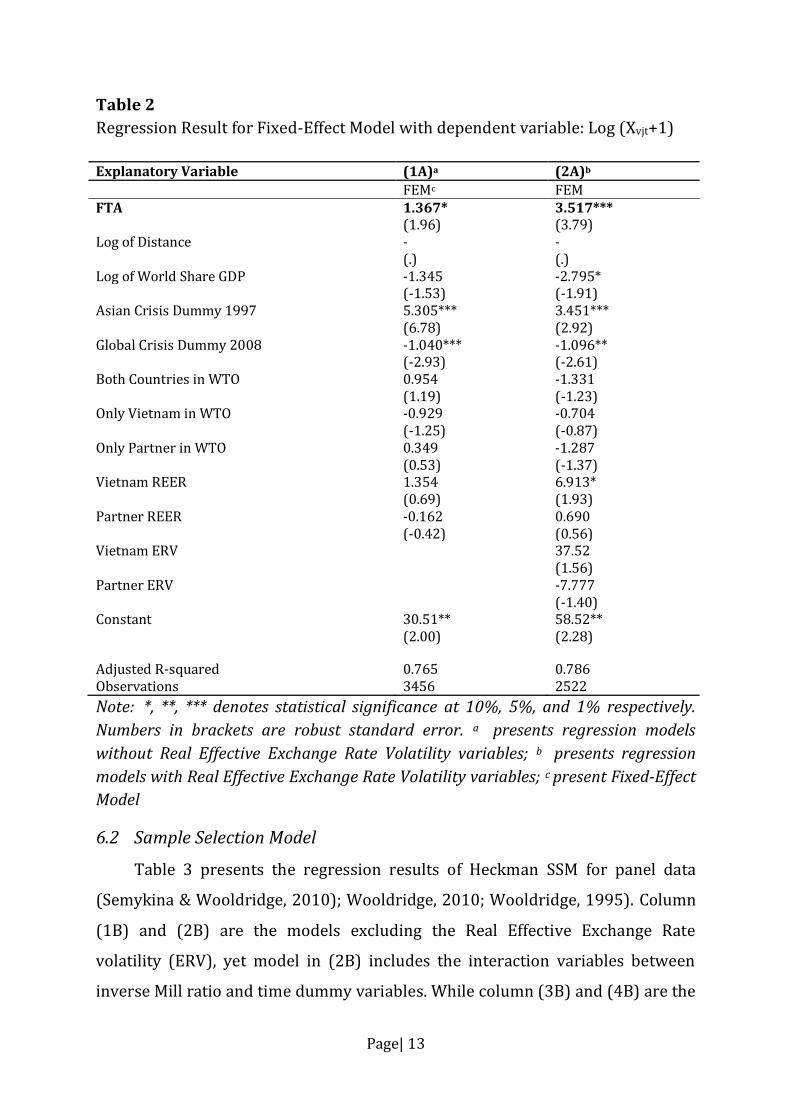
Table 2
Regression Result for Fixed-Effect Model with dependent variable: Log (Xvjt+1)
Note: *, **, *** denotes statistical significance at 10%, 5%, and 1% respectively.
Numbers in brackets are robust standard error. a presents regression models
without Real Effective Exchange Rate Volatility variables; b presents regression
models with Real Effective Exchange Rate Volatility variables; c present Fixed-Effect
Model
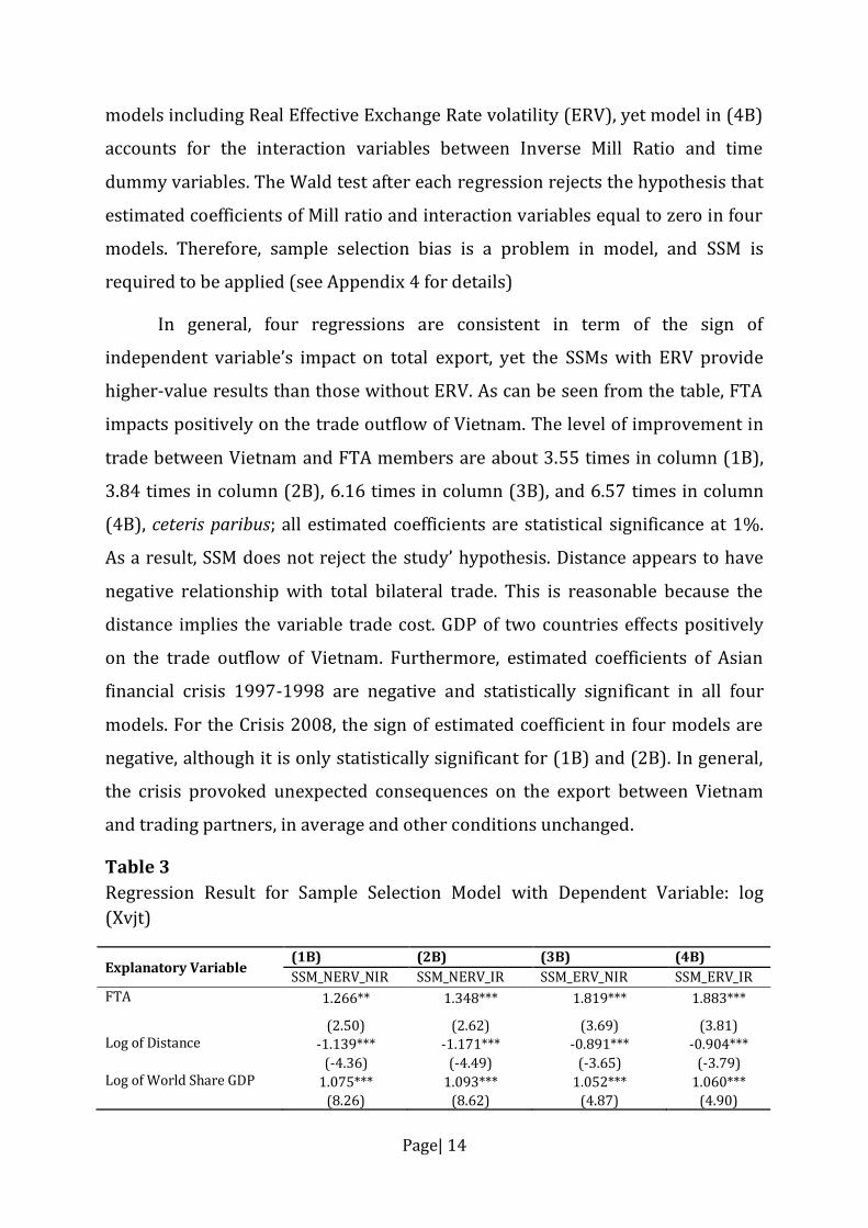
6.2 Sample Selection Model
Table 3 presents the regression results of Heckman SSM for panel data
(Semykina & Wooldridge, 2010); Wooldridge, 2010; Wooldridge, 1995). Column
(1B) and (2B) are the models excluding the Real Effective Exchange Rate
volatility (ERV), yet model in (2B) includes the interaction variables between
inverse Mill ratio and time dummy variables. While column (3B) and (4B) are the
Explanatory Variable (1A)a (2A)b
FEMc FEM FTA 1.367* 3.517*** (1.96) (3.79) Log of Distance - - (.) (.) Log of World Share GDP -1.345 -2.795* (-1.53) (-1.91) Asian Crisis Dummy 1997 5.305*** 3.451*** (6.78) (2.92) Global Crisis Dummy 2008 -1.040*** -1.096** (-2.93) (-2.61) Both Countries in WTO 0.954 -1.331 (1.19) (-1.23) Only Vietnam in WTO -0.929 -0.704 (-1.25) (-0.87) Only Partner in WTO 0.349 -1.287 (0.53) (-1.37) Vietnam REER 1.354 6.913* (0.69) (1.93) Partner REER -0.162 0.690 (-0.42) (0.56) Vietnam ERV
37.52
(1.56) Partner ERV
-7.777
(-1.40) Constant 30.51** 58.52** (2.00) (2.28) Adjusted R-squared 0.765 0.786 Observations 3456 2522
Page| 14
models including Real Effective Exchange Rate volatility (ERV), yet model in (4B)
accounts for the interaction variables between Inverse Mill Ratio and time
dummy variables. The Wald test after each regression rejects the hypothesis that
estimated coefficients of Mill ratio and interaction variables equal to zero in four
models. Therefore, sample selection bias is a problem in model, and SSM is
required to be applied (see Appendix 4 for details)
In general, four regressions are consistent in term of the sign of
independent variable’s impact on total export, yet the SSMs with ERV provide
higher-value results than those without ERV. As can be seen from the table, FTA
impacts positively on the trade outflow of Vietnam. The level of improvement in
trade between Vietnam and FTA members are about 3.55 times in column (1B),
3.84 times in column (2B), 6.16 times in column (3B), and 6.57 times in column
(4B), ceteris paribus; all estimated coefficients are statistical significance at 1%.
As a result, SSM does not reject the study’ hypothesis. Distance appears to have
negative relationship with total bilateral trade. This is reasonable because the
distance implies the variable trade cost. GDP of two countries effects positively
on the trade outflow of Vietnam. Furthermore, estimated coefficients of Asian
financial crisis 1997-1998 are negative and statistically significant in all four
models. For the Crisis 2008, the sign of estimated coefficient in four models are
negative, although it is only statistically significant for (1B) and (2B). In general,
the crisis provoked unexpected consequences on the export between Vietnam
and trading partners, in average and other conditions unchanged.
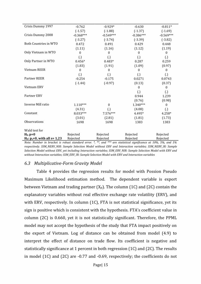
Table 3
Regression Result for Sample Selection Model with Dependent Variable: log
(Xvjt)
Explanatory Variable (1B) (2B) (3B) (4B)
SSM_NERV_NIR SSM_NERV_IR SSM_ERV_NIR SSM_ERV_IR
FTA 1.266** 1.348*** 1.819*** 1.883***
(2.50) (2.62) (3.69) (3.81) Log of Distance -1.139*** -1.171*** -0.891*** -0.904*** (-4.36) (-4.49) (-3.65) (-3.79) Log of World Share GDP 1.075*** 1.093*** 1.052*** 1.060*** (8.26) (8.62) (4.87) (4.90)
Page| 15
Crisis Dummy 1997 -0.762 -0.929* -0.630 -0.811* (-1.57) (-1.88) (-1.37) (-1.69) Crisis Dummy 2008 -0.368*** -0.549*** -0.386*** -0.569*** (-3.27) (-3.74) (-3.39) (-3.82) Both Countries in WTO 0.472 0.491 0.429 0.448 (1.11) (1.16) (1.12) (1.19) Only Vietnam in WTO 0 0 0 0 (.) (.) (.) (.) Only Partner in WTO 0.456* 0.483* 0.287 0.259 (1.83) (1.91) (1.09) (0.97) Vietnam REER 0 0 0 0 (.) (.) (.) (.) Partner REER -0.254 -0.175 0.0271 0.0743 (-1.44) (-0.97) (0.13) (0.37) Vietnam ERV
0 0
(.) (.)
Partner ERV
0.944 1.239
(0.76) (0.98)
Inverse Mill ratio 1.110*** 0 1.340*** 0 (4.31) (.) (4.08) (.) Constant 8.033*** 7.576*** 4.495* 4.258* (3.01) (2.81) (1.81) (1.73) Observations 1698 1698 1383 1383
Wald test for H0: p=0 H0: ps=0, with all s= 1,23
Rejected Rejected
Rejected Rejected
Rejected Rejected
Rejected Rejected
Note: Number in bracket is robust standard error. *, **, and *** are statistical significance at 10%, 5%, and 1%
respectively. SSM_NERV_NIR: Sample Selection Model without ERV and Interaction variables; SSM_NERV_IR: Sample
Selection Model without ERV, yet including Interaction variables; SSM_ERV_NIR: Sample Selection Model with ERV and
without Interaction variables; SSM_ERV_IR: Sample Selection Model with ERV and Interaction variables
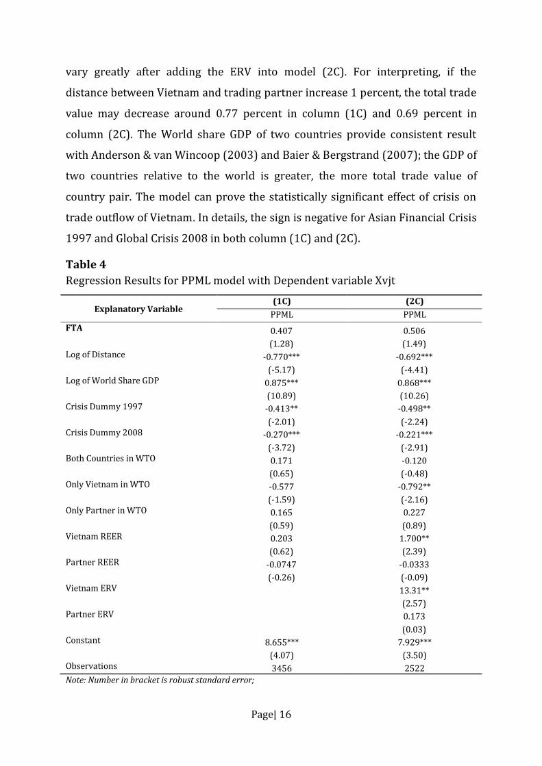
6.3 Multiplicative-Form Gravity Model
Table 4 provides the regression results for model with Possion Pseudo
Maximum Likelihood estimation method. The dependent variable is export
between Vietnam and trading partner (Xjt). The column (1C) and (2C) contain the
explanatory variables without real effective exchange rate volatility (ERV), and
with ERV, respectively. In column (1C), FTA is not statistical significance, yet its
sign is positive which is consistent with the hypothesis. FTA’s coefficient value in
column (2C) is 0.660, yet it is not statistically significant. Therefore, the PPML
model may not accept the hypothesis of the study that FTA impact positively on
the export of Vietnam. Log of distance can be obtained from model (4.9) to
interpret the effect of distance on trade flow. Its coefficient is negative and
statistically significance at 1 percent in both regression (1C) and (2C). The results
in model (1C) and (2C) are -0.77 and -0.69, respectively; the coefficients do not
Page| 16
vary greatly after adding the ERV into model (2C). For interpreting, if the
distance between Vietnam and trading partner increase 1 percent, the total trade
value may decrease around 0.77 percent in column (1C) and 0.69 percent in
column (2C). The World share GDP of two countries provide consistent result
with Anderson & van Wincoop (2003) and Baier & Bergstrand (2007); the GDP of
two countries relative to the world is greater, the more total trade value of
country pair. The model can prove the statistically significant effect of crisis on
trade outflow of Vietnam. In details, the sign is negative for Asian Financial Crisis
1997 and Global Crisis 2008 in both column (1C) and (2C).
Table 4
Regression Results for PPML model with Dependent variable Xvjt
Explanatory Variable (1C) (2C)
PPML PPML
FTA 0.407 0.506 (1.28) (1.49) Log of Distance -0.770*** -0.692*** (-5.17) (-4.41) Log of World Share GDP 0.875*** 0.868*** (10.89) (10.26) Crisis Dummy 1997 -0.413** -0.498** (-2.01) (-2.24) Crisis Dummy 2008 -0.270*** -0.221*** (-3.72) (-2.91) Both Countries in WTO 0.171 -0.120 (0.65) (-0.48) Only Vietnam in WTO -0.577 -0.792** (-1.59) (-2.16) Only Partner in WTO 0.165 0.227 (0.59) (0.89) Vietnam REER 0.203 1.700** (0.62) (2.39) Partner REER -0.0747 -0.0333 (-0.26) (-0.09) Vietnam ERV
13.31**
(2.57)
Partner ERV
0.173
(0.03)
Constant 8.655*** 7.929*** (4.07) (3.50) Observations 3456 2522
Note: Number in bracket is robust standard error;
Page| 17
*, **, and *** are statistical significance at 10%, 5%, and 1% respectively.
6.4 Discussion
In PPML estimators, the FTA has positive relationship with the export of
Vietnam, and is consistent with those in FEM and SSM. However, the value of
FTA’s coefficient is lower than coefficients and statistically insignificant in other
two methods. PPML can perform efficiently in the case of heteroscedasticity in
data, yet it is claimed to be poorly estimating in the case of frequent zero-value in
trade (Martin & Pham, 2008). This can be applied to the study’ data where the
zero values are account for nearly 50% in total observations. One indicator used
to evaluate the bias in model is GDP’s coefficient. Theoretically, the coefficient of
GDP converge to unity (Anderson & van Wincoop, 2003); and Martin and Pham
(2008) stated that if GDP’s coefficient is lower greatly than one, model may be
underestimated or downward biased. Looking at the coefficient of log World
Share GDP in PPML model, it is significant lower than one, so it may indicate that
FTA coefficient in model is downward bias. Applying to FEM models, the log
World Share GDP’s coefficient is considerably greater than one, so the FTA is
upward biased. That may be one reason for the high value of FTA coefficients in
FEM in compare to those in SSM and PPML model. Turning to the SSM, the value
of log of World Share GDP’s coefficient is nearly equal to one. This may
subjectively assert that SSM is better than other model (Linder & Groots, 2006;
Helpman, Melitz, and Rubinstein, 2007). Furthermore, the paper proves that
sample selection is appropriate for context of Vietnam export. Testing results of
collinearity of Inverse Mill Ratio show that SSM is not vulnerable. Later, the SSM
judges zero-trade value as non-random value and come from the decision of
other factor such exporter and importer while PPML and FEM do not judge zero-
trade in such way.
7 Conclusion
Empirical results from three above estimation models prove the positive
relationship between FTA and Vietnam’s export consistently. After joining the
FTA, the trade between Vietnam and its FTA-member partner increase from 3.5
Page| 18
times to 6.5 times according to SSM results. The reason for why FTA improves
the trade flow between member countries can be attribute to the elimination in
the tariffs and other trade-facilitate conditions. The tax reduction will help to
reduce the trade cost substantially. The other condition is the integration in
transit infrastructure and other custom obligation. One more reason for the
positive impact on trade of FTA can be attributed to the “natural FTA” (Krugman,
1991). Natural FTA is terminology for the FTA between countries have advantage
on geography (neighboring country, short distance), culture. The author stated
that if natural FTA is established, it will impact positively on trade flow and
welfare of members. Turning to Vietnam FTAs, most of them are with ASEAN
countries, which can become the “natural FTA”.
The government may consider the free trade agreement as a policy for trade
openness and export development. The other implication come from the study
results is the impact of the controlling variable. The distance variable indicates
that Vietnam is less likely to trade with countries are in greater distance than the
shorter ones. The trade will increase when the GDP of two countries are higher in
relative to world GDP. The controlling variables help the government to decide in
choosing trading partners.
8 Limitation and Further Research
Firstly, gravity model is “work horse” tool in estimating ex-post relationship
between trade policy and trade flow, yet in order to estimate the ex-ante effect of
FTA on trade flow of goods, the Computable General Equilibrium (CGE) is a
recommended model (Hertel et al, 2007). CGE can help to anticipate the effect of
FTA on Vietnam trade flow when the tax elimination fully in force in 2020-2027.
Other limitation of gravity model is its functional form. The log- linear form and
multiplicative form take account for non-negative observation. Thus, in the
model, dependent variables are total bilateral trade, export value, or import
value. Trade balance which is also important trade indicator cannot be included
in the model due to its negative value. The time period in data does not capture
Page| 19
the full impact of FTA on trade flow because the available of data is constrained
at the time this study is done.
The study analyzes the aggregate data on trade flow, yet the disaggregate
data also need to be taken account for because the effect of FTA will be difference
depend on sectors in the industries. Trade flow is one of the points of view in
judging the foreign trade policy. Other aspects are the welfare change (McCaig,
2011), the investment (Lakatos & Walmsley, 2012; Anderson, 2010) the labor
wage (Fukase, 2013). Those aspects are beyond the copes of this study, and they
can be a topic for future evaluation.
REFERENCE
Aitken, N. D. (1973). The effect of the EEC and EFTA on European trade: A
temporal cross-section analysis. The American Economic Review, 881-892.
Al-Rashidi, A., & Lahiri, B. (2013). The effect of exchange rate volatility on trade:
correcting for selection bias and asymmetric trade flows. Applied Economics
Letters, 20(11), 1121-1126.American Economic Review, 615-623.
Anderson, J. E., & Van Wincoop, E. (2003). Gravity with Gravitas: A Solution to the
Border Puzzle. The American Economic Review, 93(1), 170-192.
Anderson, J. E., & Van Wincoop, E. (2004). Trade costs. Journal of Economic
Literature Vol. XLII, 691-751.
Anderson, J. E. (2010). The gravity model (No. w16576). National Bureau of
Economic Research
Bahmani-Oskooee, M., & Hegerty, S. W. (2009). The effects of exchange-rate
volatility on commodity trade between the United States and Mexico. Southern
Economic Journal, 1019-1044.
Baier, S. L., & Bergstrand, J. H. (2004). Economic determinants of free trade
agreements. Journal of International Economics, 64(1), 29-63
Baier, S. L., & Bergstrand, J. H. (2007). Do free trade agreements actually increase
members' international trade?. Journal of international Economics, 71(1), 72-95.
Page| 20
Baier, S. L., & Bergstrand, J. H. (2009). < i> Bonus vetus OLS: A simple method for
approximating international trade-cost effects using the gravity equation. Journal
of International Economics, 77(1), 77-85.
Bhagwati, J. (1971). Trade-diverting customs unions and welfare-improvement:
A clarification. The Economic Journal, 580-587.
Carrère, C., & Schiff, M. (2005). On the geography of trade. Revue économique,
56(6), 1249-1274.
Chaney, T. (2008). Distorted gravity: the intensive and extensive margins of
international trade. The American Economic Review, 98(4), 1707-1721.
Crozet, M. & Koenig, P. (2010). Structural gravity equations with intensive and
extensive margins. Canadian Journal of Economics, Vol. 43, No. 1
Darvas, Zsolt (2012) Real effective exchange rates for 178 countries: a new
database. Bruegel Working Paper 2012/06
Disdier, A. C., & Head, K. (2008). The puzzling persistence of the distance effect on
bilateral trade. The Review of Economics and statistics, 90(1), 37-48.
Fukase, E., & Martin, W. (2001). A Quantitative evaluation of Vietnam's accession
to the ASEAN Free Trade Area. Journal of Economic Integration, 545-567.
Fukase, E. (2013). Export Liberalization, Job Creation, and the Skill Premium:
Evidence from the US–Vietnam Bilateral Trade Agreement (BTA). World
Development, 41, 317-337.
Head, K., & Mayer, T. (2013). Gravity equations: Workhorse, toolkit, and
cookbook. Handbook of international economics, 4.
Helpman, E., Melitz, M., & Rubinstein, Y. (2007). Estimating trade flows: Trading
partners and trading volumes (No. w12927). National Bureau of Economic
Research.
Hertel, T., Hummels, D., Ivanic, M., & Keeney, R. (2007). How confident can we be
of CGE-based assessments of free trade agreements?. Economic Modelling, 24(4),
611-635.
Heckman, J. J. (1979). Sample selection bias as a specification error.
Econometrica: Journal of the econometric society, 153-161.
Hur, J., Alba, J. D., & Park, D. (2010). Effects of hub-and-spoke free trade
agreements on trade: A panel data analysis. World Development, 38(8), 1105-111
Page| 21
Johnson, H. G. (1974). Trade-diverting customs unions: A comment. The
Economic Journal, 618-621.
Jugurnath, B., Stewart, M., & Brooks, R. (2007). Asia/Pacific regional trade
agreements: an empirical study. Journal of Asian Economics, 18(6), 974-987.
Krugman, P. (1991). The move toward free trade zones. Economic Review, 76(6),
5.
Lakatos, C., & Walmsley, T. (2012). Investment creation and diversion effects of
the ASEAN–China free trade agreement. Economic Modelling, 29(3), 766-779.
Linders, G. J. M., & De Groot, H. L. (2006). Estimation of the gravity equation in the
presence of zero flows (No. 06-072/3). Tinbergen Institute Discussion Paper.
Lipsey, R. G. (1957). The theory of customs unions: trade diversion and welfare.
Economica, 40-46
Madden, D. (2008). Sample selection versus two-part models revisited: The case
of female smoking and drinking. Journal of Health Economics, 27(2), 300-307.
Martínez-Zarzoso, I. (2013). The log of gravity revisited. Applied Economics,
45(3), 311-327.
Martin, W., & Pham, C. S. (2008). Estimating the gravity equation when zero trade
flows are frequent.mimeo
McCaig, B. (2011). Exporting out of poverty: Provincial poverty in Vietnam and
US market access. Journal of International Economics, 85(1), 102-113
McCallum, J. (1995). National borders matter: Canada-US regional trade patterns.
The American Economic Review, 615-623.
McKenzie, M. D. (1999). The impact of exchange rate volatility on international
trade flows. Journal of Economic Surveys, 13(1), 71-106.
Rose, A. K., & Van Wincoop, E. (2001). National money as a barrier to
international trade: The real case for currency union. American Economic Review,
386-390.
Semykina, A., & Wooldridge, J. M. (2010). Estimating panel data models in the
presence of endogeneity and selection. Journal of Econometrics, 157(2), 375-380.
Silva, J. S., & Tenreyro, S. (2006). The log of gravity. The Review of Economics and
statistics, 88(4), 641-658.
Page| 22
Tenreyro, S. (2007). On the trade impact of nominal exchange rate volatility.
Journal of Development Economics, 82(2), 485-508.
Thai, T. D. (2006). A gravity model for trade between Vietnam and twenty-three
European countries.
Wooldridge, J. M. (1995). Selection corrections for panel data models under
conditional mean independence assumptions. Journal of econometrics, 68(1), 115-
132.
Wooldridge, J. M. (2010). Econometric analysis of cross section and panel data.
London: MIT press.
Yang, S., & Martinez-Zarzoso, I. (2013). A panel data analysis of trade creation
and trade diversion effects: The case of ASEAN–China Free Trade Area. China
Economic Review 29 (2014), 138–151
Page| 23
Appendix 1. List of countries
Afghanistan, Islamic Republic of
Bosnia and Herzegovina
China, P.R.: Mainland
Guatemala Kuwait Morocco Russian Federation
Tajikistan
Albania Botswana Denmark Guinea Kyrgyz Republic Mozambique Rwanda Tanzania
Algeria Brazil Dominica Guinea-Bissau Lao People's Democratic Republic
Myanmar Samoa Timor-Leste, Dem. Rep. of
American Samoa Brunei Darussalam Dominican Republic
Guyana Latvia Namibia Saudi Arabia Togo
Antigua and Barbuda
Bulgaria Ecuador Haiti Lebanon Nepal Senegal Tonga
Angola Burkina Faso Egypt Honduras Lesotho Netherlands Seychelles Tunisia Argentina Burundi El Salvador Hungary Liberia New Zealand Sierra Leone Turkey Armenia, Republic of
Cabo Verde Equatorial Guinea
Iceland Libya Nicaragua Singapore Turkmenistan
Aruba Cambodia Eritrea India Lithuania Niger Slovak Republic Tuvalu Australia Cameroon Estonia Indonesia Luxembourg Nigeria Slovenia Thailand
Austria Canada Ethiopia Iran, Islamic Republic of
Macedonia, FYR Norway Solomon Islands Trinidad and Tobago
Azerbaijan, Republic of
Colombia European Union Iraq Madagascar Oman South Africa Uganda
Bahamas, The Comoros Fiji Ireland Malawi Pakistan Spain Ukraine
Bahrain, Kingdom of Congo, Democratic Republic of
Finland Israel Malaysia Palau Sri Lanka United Arab Emirates
Bangladesh Congo, Republic of France Italy Maldives Panama St. Kitts and Nevis United Kingdom Barbados Costa Rica Gabon Jamaica Mali Papua New Guinea St. Lucia United States
Belarus Cote d'Ivoire Gambia, The Japan Malta Paraguay St. Vincent and the Grenadines
Uruguay
Belgium Croatia Georgia Jordan Mauritania Peru Sudan Uzbekistan Belize Cuba Germany Jordan Mauritius Poland Suriname Vanuatu
Benin Cyprus Ghana Kazakhstan Mexico Portugal Swaziland Venezuela, Republica Bolivariana de
Bermuda Czech Republic Greece Kenya Moldova Philippines Sweden Yemen, Republic of Bhutan Chad Greenland Kiribati Montenegro Qatar Switzerland Zambia
Bolivia Chile Grenada Korea, Republic of Mongolia Romania Syrian Arab Republic
Zimbabwe
Page| 24
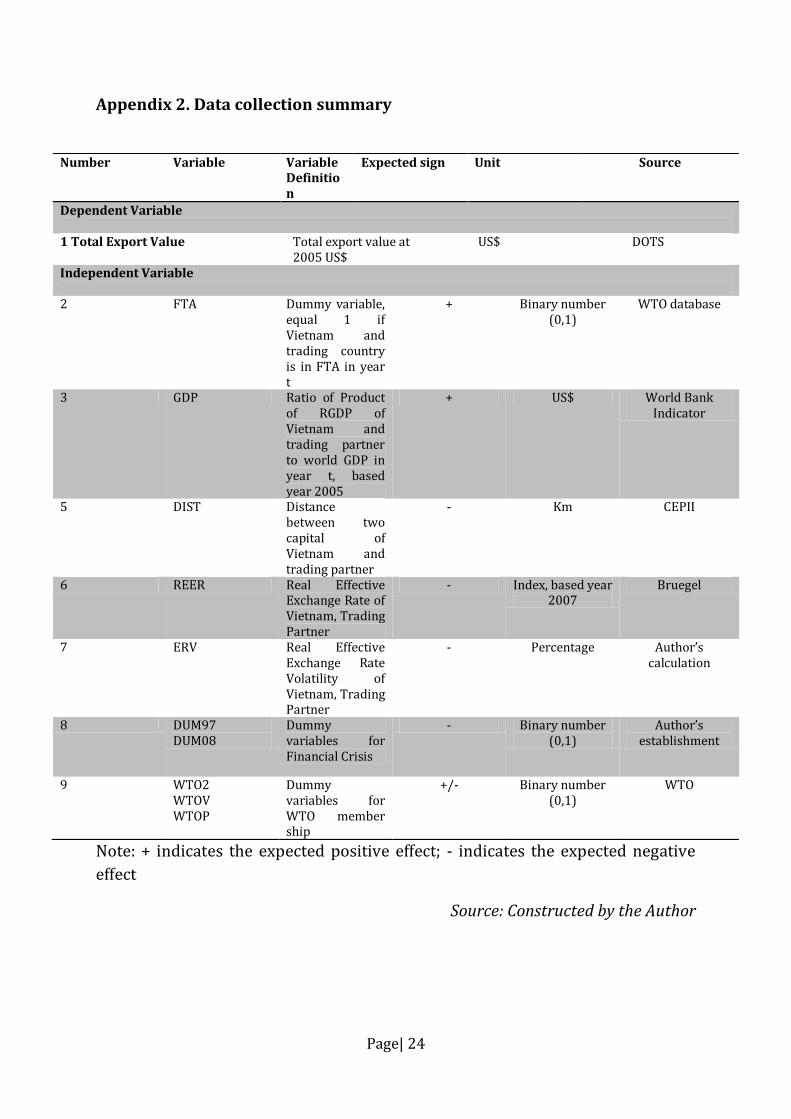
Appendix 2. Data collection summary
Note: + indicates the expected positive effect; - indicates the expected negative
effect
Source: Constructed by the Author
Number Variable Variable Definition
Expected sign Unit Source
Dependent Variable 1 Total Export Value Total export value at
2005 US$ US$ DOTS
Independent Variable 2 FTA Dummy variable,
equal 1 if Vietnam and trading country is in FTA in year t
+ Binary number (0,1)
WTO database
3 GDP Ratio of Product of RGDP of Vietnam and trading partner to world GDP in year t, based year 2005
+ US$ World Bank Indicator
5 DIST Distance between two capital of Vietnam and trading partner
- Km CEPII
6 REER Real Effective Exchange Rate of Vietnam, Trading Partner
- Index, based year 2007
Bruegel
7 ERV Real Effective Exchange Rate Volatility of Vietnam, Trading Partner
- Percentage Author’s calculation
8 DUM97 DUM08
Dummy variables for Financial Crisis
- Binary number (0,1)
Author’s establishment
9 WTO2 WTOV WTOP
Dummy variables for WTO member ship
+/- Binary number (0,1)
WTO
Page| 25
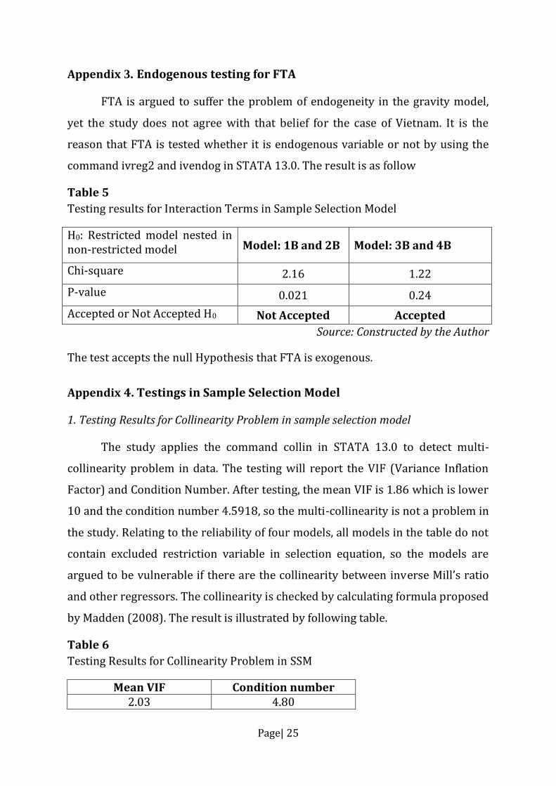
Appendix 3. Endogenous testing for FTA
FTA is argued to suffer the problem of endogeneity in the gravity model,
yet the study does not agree with that belief for the case of Vietnam. It is the
reason that FTA is tested whether it is endogenous variable or not by using the
command ivreg2 and ivendog in STATA 13.0. The result is as follow
Table 5
Testing results for Interaction Terms in Sample Selection Model
H0: Restricted model nested in non-restricted model Model: 1B and 2B Model: 3B and 4B
Chi-square 2.16 1.22
P-value 0.021 0.24
Accepted or Not Accepted H0 Not Accepted Accepted
Source: Constructed by the Author
The test accepts the null Hypothesis that FTA is exogenous.
Appendix 4. Testings in Sample Selection Model
1. Testing Results for Collinearity Problem in sample selection model
The study applies the command collin in STATA 13.0 to detect multi-
collinearity problem in data. The testing will report the VIF (Variance Inflation
Factor) and Condition Number. After testing, the mean VIF is 1.86 which is lower
10 and the condition number 4.5918, so the multi-collinearity is not a problem in
the study. Relating to the reliability of four models, all models in the table do not
contain excluded restriction variable in selection equation, so the models are
argued to be vulnerable if there are the collinearity between inverse Mill’s ratio
and other regressors. The collinearity is checked by calculating formula proposed
by Madden (2008). The result is illustrated by following table.
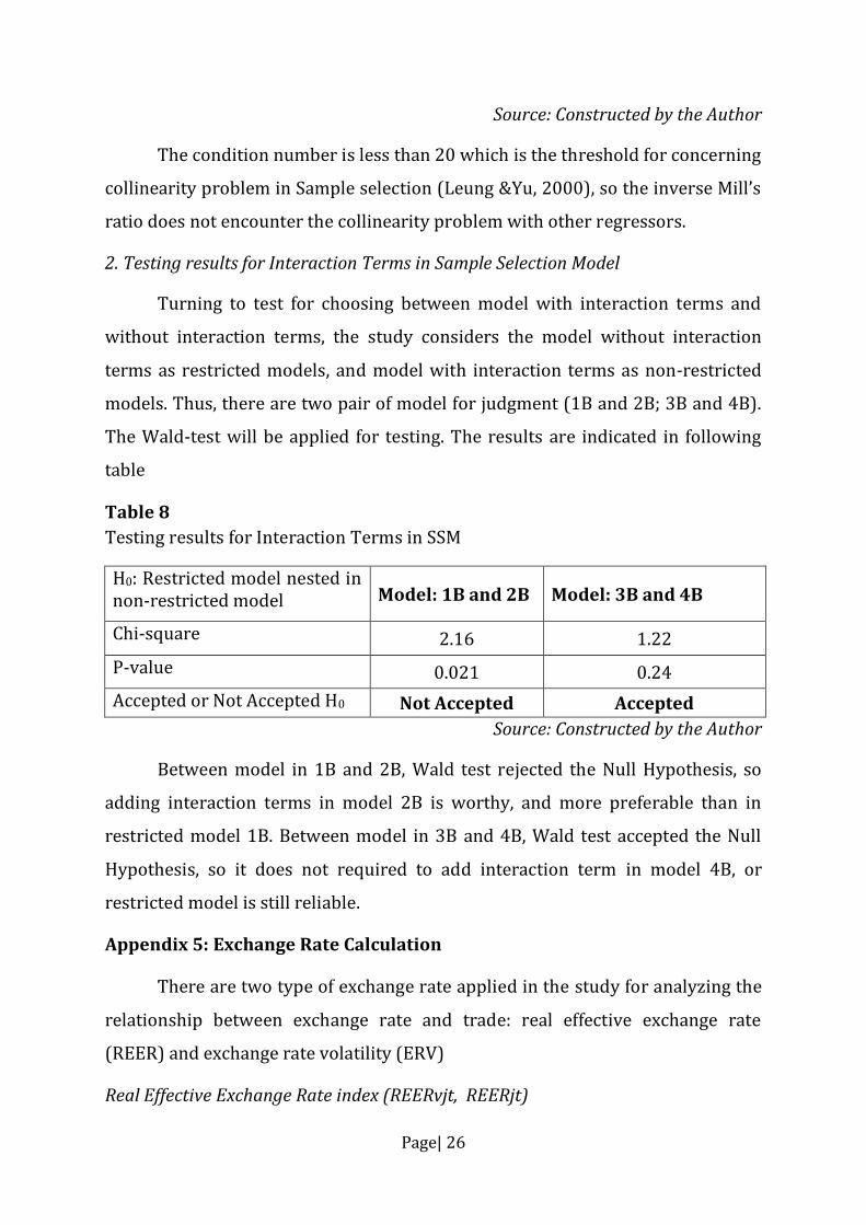
Table 6
Testing Results for Collinearity Problem in SSM
Mean VIF Condition number 2.03 4.80
Page| 26
Source: Constructed by the Author
The condition number is less than 20 which is the threshold for concerning
collinearity problem in Sample selection (Leung &Yu, 2000), so the inverse Mill’s
ratio does not encounter the collinearity problem with other regressors.
2. Testing results for Interaction Terms in Sample Selection Model
Turning to test for choosing between model with interaction terms and
without interaction terms, the study considers the model without interaction
terms as restricted models, and model with interaction terms as non-restricted
models. Thus, there are two pair of model for judgment (1B and 2B; 3B and 4B).
The Wald-test will be applied for testing. The results are indicated in following
table
Table 8
Testing results for Interaction Terms in SSM
H0: Restricted model nested in non-restricted model Model: 1B and 2B Model: 3B and 4B
Chi-square 2.16 1.22
P-value 0.021 0.24
Accepted or Not Accepted H0 Not Accepted Accepted
Source: Constructed by the Author
Between model in 1B and 2B, Wald test rejected the Null Hypothesis, so
adding interaction terms in model 2B is worthy, and more preferable than in
restricted model 1B. Between model in 3B and 4B, Wald test accepted the Null
Hypothesis, so it does not required to add interaction term in model 4B, or
restricted model is still reliable.
Appendix 5: Exchange Rate Calculation
There are two type of exchange rate applied in the study for analyzing the
relationship between exchange rate and trade: real effective exchange rate
(REER) and exchange rate volatility (ERV)
Real Effective Exchange Rate index (REERvjt, REERjt)
Page| 27
The study will use real effective exchange rate index (REER) as a proxy for
controlling the impact of exchange rate on trade flow between Vietnam and her
partner. REER is obtained from Nominal Effective Exchange Rate (NEER) deflated
by the relative price between calculating country and its trading partners. It is
consider as the measurement of the change of domestic currency in response to
bundle of trading partners.
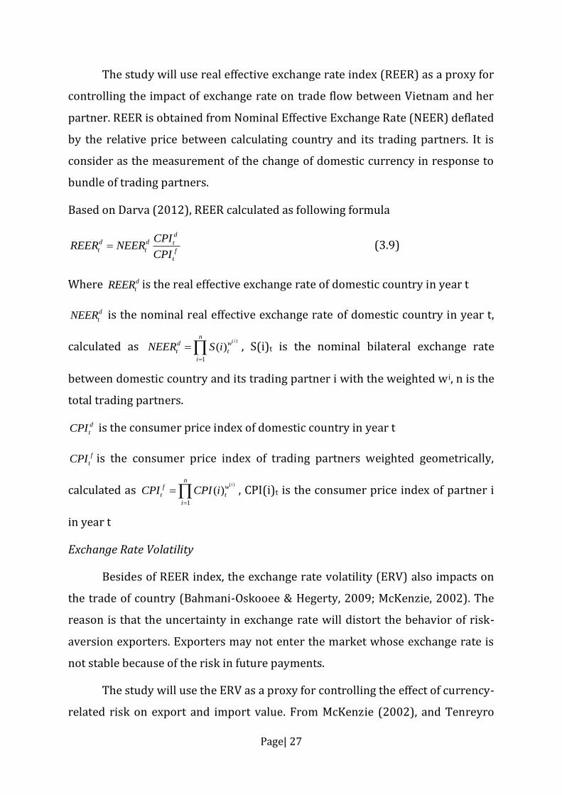
Based on Darva (2012), REER calculated as following formula
dd d tt t f
t
CPIREER NEER
CPI (3.9)
Where d
tREER is the real effective exchange rate of domestic country in year t
d
tNEER is the nominal real effective exchange rate of domestic country in year t,
calculated as ( )
1
( )i
nd w
t t
i
NEER S i
, S(i)t is the nominal bilateral exchange rate
between domestic country and its trading partner i with the weighted wi, n is the
total trading partners.
d
tCPI is the consumer price index of domestic country in year t
f
tCPI is the consumer price index of trading partners weighted geometrically,
calculated as ( )
1
( )i
nf w
t t
i
CPI CPI i
, CPI(i)t is the consumer price index of partner i
in year t
Exchange Rate Volatility
Besides of REER index, the exchange rate volatility (ERV) also impacts on
the trade of country (Bahmani-Oskooee & Hegerty, 2009; McKenzie, 2002). The
reason is that the uncertainty in exchange rate will distort the behavior of risk-
aversion exporters. Exporters may not enter the market whose exchange rate is
not stable because of the risk in future payments.
The study will use the ERV as a proxy for controlling the effect of currency-
related risk on export and import value. From McKenzie (2002), and Tenreyro
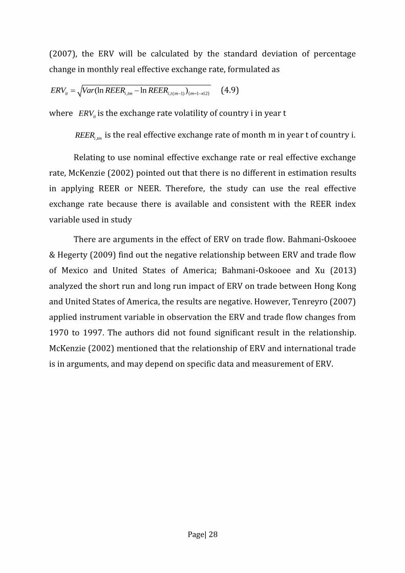
Page| 28
(2007), the ERV will be calculated by the standard deviation of percentage
change in monthly real effective exchange rate, formulated as
, , ( 1) { 1 12}(ln ln )it i tm i t m mERV Var REER REER (4.9)
where itERV is the exchange rate volatility of country i in year t
,i tmREER is the real effective exchange rate of month m in year t of country i.
Relating to use nominal effective exchange rate or real effective exchange
rate, McKenzie (2002) pointed out that there is no different in estimation results
in applying REER or NEER. Therefore, the study can use the real effective
exchange rate because there is available and consistent with the REER index
variable used in study
There are arguments in the effect of ERV on trade flow. Bahmani-Oskooee
& Hegerty (2009) find out the negative relationship between ERV and trade flow
of Mexico and United States of America; Bahmani-Oskooee and Xu (2013)
analyzed the short run and long run impact of ERV on trade between Hong Kong
and United States of America, the results are negative. However, Tenreyro (2007)
applied instrument variable in observation the ERV and trade flow changes from
1970 to 1997. The authors did not found significant result in the relationship.
McKenzie (2002) mentioned that the relationship of ERV and international trade
is in arguments, and may depend on specific data and measurement of ERV.