WORKING PAPER SERIESFED

ERAL

RES

ERVE

BAN

K o

f ATL

ANTA

The Impact of Medical and Nursing Home Expenses and Social Insurance Policies on Savings and Inequality Karen A. Kopecky and Tatyana Koreshkova Working Paper 2010-19 December 2010

The authors thank Arpad Abraham, Rui Castro, Eric French, Joao Gomes, Jonathan Heathcote, Narayana Kocherlakota, Leonardo Martinez, Jose Victor Rios-Rull, Juan Sanchez, John Karl Scholz, Ananth Seshadri, Richard Suen, and Motohiro Yogo for helpful comments and Kai Xu for excellent research assistance. They also thank seminar participants at the Atlanta and Minneapolis Federal Reserve Banks, the Université de Montréal, the University of North Carolina at Chapel Hill, the University of Western Ontario, University of Wisconsin-Madison, and the Wharton School and conference participants at the 2008 Canadian Macro Study Group, the 2007 and 2008 Wegmans Conferences at the University of Rochester, the 2008 Conference on Income Distribution and Family at the University of Kiel, the 2009 meeting of the Society for Economic Dynamics, and the 2009 Conference on Health and the Macroeconomy at the Laboratory for Aggregate Economics and Finance at the University of California, Santa Barbara. The views expressed here are the authors’ and not necessarily those of the Federal Reserve Bank of Atlanta or the Federal Reserve System. Any remaining errors are the authors’ responsibility. Please address questions regarding content to Karen A. Kopecky, Economist, Research Department, Federal Reserve Bank of Atlanta, 1000 Peachtree Street, N.E., Atlanta, GA 30309-4470, 404-498-8974, karen.kopecky@atl.frb.org, or Tatyana Koreshkova, Assistant Professor, Department of Economics, Concordia University, 1455 de Maisonneuve Boulevard West, Montreal, Quebec, Canada, H3G 1M8, 514-848-2424 ext. 3923, tkoreshk@alcor.concordia.ca. Federal Reserve Bank of Atlanta working papers, including revised versions, are available on the Atlanta Fed’s Web site at frbatlanta.org/pubs/WP/. Use the WebScriber Service at frbatlanta.org to receive e-mail notifications about new papers.

FEDERAL RESERVE BANK of ATLANTA WORKING PAPER SERIES

The Impact of Medical and Nursing Home Expenses and Social Insurance Policies on Savings and Inequality Karen A. Kopecky and Tatyana Koreshkova Working Paper 2010-19 December 2010 Abstract: We consider a life-cycle model with idiosyncratic risk in labor earnings, out-of-pocket medical and nursing home expenses, and survival. Partial insurance is available through welfare, Medicaid, and social security. Calibrating the model to the United States, we find that 12 percent of aggregate savings is accumulated to finance and self-insure against old-age health expenses given the absence of complete public health care for the elderly and that nursing home expenses play an important role in the savings of the wealthy and on aggregate. Moreover, we find that the aggregate and distributional effects of public health care provision are highly dependent on the availability of other programs making up the social insurance system. JEL classification: E21, H31, H53, I18, I38 Key words: out-of-pocket medical expenses, nursing home costs, means-tested social insurance, life-cycle savings, wealth inequality, social security

The Impact of Medical and Nursing Home Expenses and Social Insurance Policies on

Savings and Inequality

1 Introduction

With aging populations and soaring medical costs, health care has never been of greater concern to

policy-makers and individuals. The elderly in the United States in particular face large, volatile out-

of-pocket health expenses that increase quickly with age as Medicare only provides limited coverage

of some health care costs. In 2000, average out-of-pocket (OOP) expenditure for households with

heads aged 65 and over was approximately $3,000 with a standard deviation of over $6,000.1

Furthermore, individuals aged 85 years and over spent more than twice as much on medical care

as those aged 65 to 74. With high costs and limited insurance options, nursing home expenses are

a significant driver of large and highly skewed OOP expenditures. Rates for nursing home care in

2005 were in the range of $60,000 to $75,000 per year and a significant fraction of the elderly can

face nursing home costs that persist for years. Of the eighteen percent of 65-year-olds who will

require nursing home care at some point in their lifetime, nearly half will require more than 3 years

of care, and nearly a quarter will require more than 5 years.2

The two main ways in which the elderly finance medical and nursing home expenses not covered

by Medicare and insure against the risk of large OOP expenses are through private savings and

social insurance programs. A number of studies have emphasized the importance of OOP health

expenses and their risks for understanding individual saving behavior.3 The objective of this

paper is to quantitatively assess the impact of medical and nursing home expenses and their social

insurance for savings and inequality. In particular, we ask how the lack of complete public coverage

of both medical and nursing home expenses in the U.S. impacts aggregate and distributional saving

behavior and consumption inequality. We then assess the extent to which our findings depend

on the degree of insurance provided through other social insurance programs by examining the

interaction of public health care with public welfare for workers, Medicaid and old-age welfare, and

1Authors calculation based on data from the 2000 Health and Retirement Study.2Source for nursing home costs: Metlife Market Survey of Nursing Home and Assisted Living Costs. Source for

nursing home usage statistics: Dick, Garber and MaCurdy (1994)3Such as Kotlikoff (1988), Hubbard et al. (1995), Palumbo (1999), Scholz et al. (2006), and De Nardi et al.

(2006).

1

social security.

To this end we build a general equilibrium, life-cycle model with overlapping generations of

individuals and population growth. Individuals work till age 65 and then retire. During the working

stage of their lives, individuals face earnings uncertainty. Retired individuals face uncertainty with

respect to their survival as well as medical and nursing home expenses. Different histories of

earnings give rise to cross-sectional wealth inequality well before retirement. We assume that

individuals cannot borrow and that there are no markets to insure against labor market, medical,

nursing home, or survival risk. Partial insurance, however, is available through three programs run

by the government: a progressive pay-as-you-go social security program, a welfare program that

guarantees a minimum level of consumption to workers, and a Medicaid-like social safety net that

guarantees a minimum consumption level to retirees with impoverishing medical and nursing home

expenses. We allow the insured consumption floor to be specific to the type of the health shock

(medical or nursing home).

We calibrate the benchmark economy to a set of cross-sectional moments from the U.S. data.

To pin down the stochastic process for medical costs, we use data from the Health and Retirement

Study. Since in the data we only observe OOP health expenditures and not total expenditures

(before Medicaid subsidies), we cannot directly infer the medical cost process. Instead, we cali-

brate the process so that the distribution of OOP expenditures generated by the model matches

the one observed in the data. Furthermore, our calibration procedure allows us to infer the level of

consumption provided under public nursing home care. In particular, we find that the consumption

floor guaranteed by Medicaid to a nursing home resident lies below the consumption floor guar-

anteed to a non-nursing home resident. In other words, Medicaid provides differential insurance

against medical versus nursing home expense risk. We interpret this differential as reflecting a lower

quality of life provided by public nursing home care relative to receiving public assistance while

living at home.

Our main results are as follows. First, we find that while, surprisingly, the lack of public

health care has little effect on either aggregate wealth or consumption inequality, it implies that

12 percent of aggregate capital is accumulated to finance and self-insure against old-age health

expenses. Moreover even though OOP nursing home expenses are only one fifth of total OOP

expenses, they account for half of the additional savings accumulated due to the absence of public

2

coverage. This is because nursing home expenses are one of the largest shocks in the model economy,

the most persistent, and the least insured by the government and thus they are riskier than medical

expenses and generate a relatively higher level of precautionary savings. Furthermore, nursing home

expenses play a much larger role in the savings of the rich relative to the poor. The decline in asset

holdings of the top two permanent earnings quintiles accounts for three quarters of the aggregate

reduction in savings when public health care is introduced, and this decline is driven by the public

coverage of OOP nursing home expenses. Moreover, we find that general equilibrium is important

as partial equilibrium analysis overstates the change in the capital stock due to public health care

by almost 60 percent.

Second, we find that the impact of public health care on savings and inequality is highly sensitive

to features of other social insurance programs such as safety nets for the young and old, and pay-

as-you-go social security. In particular, we find that providing low quality and/or means-tested

nursing home care generates substantial savings by wealthier individuals and promotes wealth and

consumption inequality among the elderly. Moreover, the relationships between the extent of social

insurance and savings and inequality are complex and highly dependent on the eligibility criteria

(universal or means-tested) to receive social assistance from a particular government program.

Given that there is a substantial amount of variation across countries with respect to the type and

extent of social insurance provided, these results suggest that our framework may be useful for

studying cross-country differences in savings and wealth inequality.

Third, we find that between the two means-tested government assistance programs – welfare for

workers and Medicaid/welfare for retirees – Medicaid and old-age welfare have a much larger impact

on aggregate wealth accumulation. This is explained by the presence of OOP health expenses and

the timing of earnings versus health expense shocks. Essentially, savings for old-age health expenses

provide a significant buffer against additional earnings risk introduced by the removal of its social

insurance.

Fourth, we find that while precautionary savings for health expense risk plays a relatively minor

role, accounting for approximately 4 percent of aggregate capital, precautionary savings against

uncertainty about survival risk coupled with an upward-sloping mean health expenditure profile

is substantial, accounting for 15 percent of aggregate capital. That is, precautionary savings are

driven by lifetime OOP health expense risk, rather than by the uncertainty about health expenses

3

at any given age.

Our study is the first to assess the impact of limited public coverage of both medical and

nursing home expenses on savings and inequality in a full life-cycle, general equilibrium framework.

It extends a large literature on life-cycle savings and wealth inequality (see Castaneda et al. for an

excellent survey). While most of this literature focuses on idiosyncratic income risk, our analysis

incorporates medical and nursing home expense risk. Works most closely related to our analysis

are by Ameriks et al. (2007), Hubbard et al. (1995), Scholz et al. (2006), and De Nardi et al.

(2006). Long-term care costs are explicitly modeled in Ameriks et al. (2007) with an objective

to disentangle the precautionary savings motive from the bequest motive using a strategic survey.

Safety nets are examined in a partial equilibrium framework in Hubbard et al. (1995) and De

Nardi et al. (2006). Our objective is different from these studies in that we examine the impact for

aggregate savings and wealth inequality of the lack of public health care for medical and nursing

home expenses and the interaction of public health care with other social insurance programs.

Give that this is one of the first attempts to explicitly model nursing home costs in a general

equilibrium, life-cycle, heterogeneous-agent model, for the sake of a transparent analysis, we chose

to abstract from a number of features, leaving them for future research. We now discuss a few of

these features in more detail. First, we do not model the Medicare program since it is not necessary

in order to achieve our objective. We do not model the demand for health care, but treat health

expenses as exogenous shocks. In such an environment the presence of an entitlement program

such as Medicare has no effect on individual behavior apart from the tax distortions induced by

its public finance.4 Furthermore, Medicare expenses are not observed in our health expense data

source, the Health and Retirement Study, which is the primary data source for health expenses of

the elderly.

Second economic agents in our model are a combination of a household and an individual (in

the model, we refer to them as individuals). This is a compromise between model simplicity and

data availability that we are not the first to make (Hubbard, Skinner, and Zeldes (1995) is the

closest example to us). The main tradeoff is that, on the one hand, the distributions of earnings

4Explicitly modeling Medicare would be necessary to analyze the impact of removing the program, reducing itscoverage, or changing its public finance. However, this type of analysis is not the goal of the current paper. SeeAttanasio et al. (2008) for an example of such an analysis in a general equilibrium model which does not have explicitnursing home risk.

4

and wealth – two crucial dimensions of heterogeneity for the questions we address – are a result of

joint decision-making within the household, and as such, they make more sense at the household

level (even apart from the fact that the wealth distribution is only observed at the household level).

Whereas, on the other hand, nursing home entry and survival risk is individual and data on nursing

home residents is observed for individuals. Thus we view our agents as households when working

and as individuals when retired. This assumption is consistent with the fact that while the majority

of households with heads aged 25 to 64 consist of married couples, over 60 percent of households

with heads 65 and over are single individuals.5 Furthermore, we find that the extent of earnings

risk in the model, which is the only part we calibrate using household level data, is of secondary

importance for savings and inequality to the presence of OOP medical and nursing home expenses,

their risks, and survival risk.

The paper proceeds as follows. The size and extent of social insurance for health expenses in

the U.S. are documented in Section 2. In Section 3, the benchmark model is presented. Section 4

explains the calibration of the benchmark economy. In Section 5 we compare the wealth distribution

generated by the model, and not targeted by the calibration procedure, to the one for the U.S. from

the data. We find that the model does an excellent job at generating a wealth distribution that

is in line with the data, and that the large degree of wealth inequality generated by the model is

primarily due to the presence of means-tested social insurance. In Section 6, we assess the impact of

the lack of public health care for medical and nursing home expenses on savings and inequality and

then examine the interaction of other social insurance programs with the effects of public health

care. Finally, Section 7 concludes.

2 Evidence on Health Expenses and Public Insurance

In this section we first discuss the size, composition and public insurance coverage of health expen-

ditures on aggregate, and then document the distribution of these expenditures across the elderly.

Among personal health expenditures, defined as national health expenditures net of expenditures

on medical construction and medical research, we distinguish between medical and nursing home

expenditures. Medical expenditures include expenditures on hospital, physician and clinical ser-

5Explicitly modeling marriage and nursing home expense risk is significantly more complicated for a number ofreasons that are mentioned in more detail in Section 7.

5

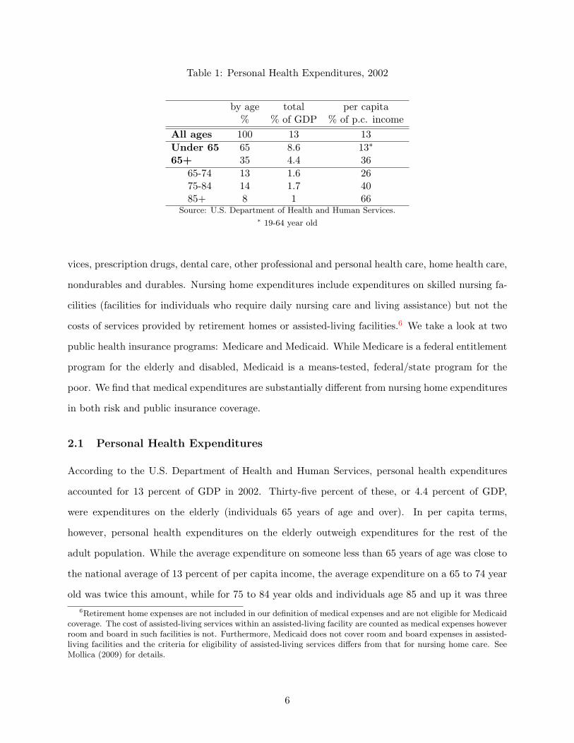
Table 1: Personal Health Expenditures, 2002

by age total per capita% % of GDP % of p.c. income

All ages 100 13 13

Under 65 65 8.6 13∗

65+ 35 4.4 36

65-74 13 1.6 2675-84 14 1.7 4085+ 8 1 66

Source: U.S. Department of Health and Human Services.∗ 19-64 year old

vices, prescription drugs, dental care, other professional and personal health care, home health care,

nondurables and durables. Nursing home expenditures include expenditures on skilled nursing fa-

cilities (facilities for individuals who require daily nursing care and living assistance) but not the

costs of services provided by retirement homes or assisted-living facilities.6 We take a look at two

public health insurance programs: Medicare and Medicaid. While Medicare is a federal entitlement

program for the elderly and disabled, Medicaid is a means-tested, federal/state program for the

poor. We find that medical expenditures are substantially different from nursing home expenditures

in both risk and public insurance coverage.

2.1 Personal Health Expenditures

According to the U.S. Department of Health and Human Services, personal health expenditures

accounted for 13 percent of GDP in 2002. Thirty-five percent of these, or 4.4 percent of GDP,

were expenditures on the elderly (individuals 65 years of age and over). In per capita terms,

however, personal health expenditures on the elderly outweigh expenditures for the rest of the

adult population. While the average expenditure on someone less than 65 years of age was close to

the national average of 13 percent of per capita income, the average expenditure on a 65 to 74 year

old was twice this amount, while for 75 to 84 year olds and individuals age 85 and up it was three

6Retirement home expenses are not included in our definition of medical expenses and are not eligible for Medicaidcoverage. The cost of assisted-living services within an assisted-living facility are counted as medical expenses howeverroom and board in such facilities is not. Furthermore, Medicaid does not cover room and board expenses in assisted-living facilities and the criteria for eligibility of assisted-living services differs from that for nursing home care. SeeMollica (2009) for details.

6

Table 2: Personal Health Expenditures by How Financed for Individuals Ages 65 and Over, 2002

Source of Payment % of total % of GDP

All 100 4.4

Private 34 1.5Out-of-pocket∗ 16 0.7Private Insurance 16 0.7Other 2 0.1

Public 66 2.9Medicare 48 2.1Medicaid 14 0.6Other 4 0.2

Source: U.S. Department of Health and Human Services.

times and five times this amount, respectively. Personal health expenditures by age as a percent of

GDP and per capita income are provided in Table 1.

How were the large expenditures on the elderly financed? Table 2 shows that 34 percent of total

personal health expenditures, or 1.5 percent of GDP, were privately financed either out-of-pocket,

with private insurance or through other means, while the remaining 66 percent, or 2.9 percent

of GDP, were publicly financed by either Medicare, Medicaid, or other public programs. Note

that Medicaid finances a substantial portion – 14 percent – of the elderly’s medical expenses, or 0.6

percent of GDP. Table 3 shows that medical expenditures of the elderly not covered by Medicare are

primarily funded by private sources: either OOP directly or indirectly through insurance payments.

Private payments of the elderly accounted for 12.3 percent of per capita GDP while Medicaid

accounted for 5.2 percent. In addition, both private and Medicaid payments for medical care as a

share of income per capita increase with age. Note that Medicaid’s share of total expenditures net

of Medicare increases with age as well: it is 22 percent for 65 to 74 year-olds, 29 percent for 75

to 84 year-olds, and 41 percent for individuals ages 85 and up. Older individuals are more likely

to have large medical expenditures and to be impoverished by large OOP medical expenditures at

earlier ages, making them eligible for Medicaid transfers.

2.2 Nursing Home Care

Nursing home costs are one of the largest OOP health expenses faced by the elderly. According to

the Medicare Current Beneficiary Survey, in 2002 nursing home care accounted for 19 percent of

7

personal health expenditures for individuals ages 65 and over and 0.85 percent of GDP. However,

since only 4 percent of the elderly resided in nursing homes (Federal Agency Forum of Aging-

Related Statistics), the cost per nursing home resident was substantially higher – 190 percent of

income per capita. Consistent with these statistics, the Metlife Market Survey of Nursing Home

and Assisted Living Costs reports that the average daily rate for a private room in a nursing home

in 2005 was $203 or $74,095 annually while the average daily rate for a semiprivate room was $176

or $64,240 annually.

Nursing home expenses in the U.S. are predominantly financed either OOP or publicly by

either the Medicare or Medicaid programs. However, Medicare coverage for nursing home care

is limited in that it only covers costs for the first six months of care and partially subsidizes the

next six months. Thus while Medicare is the primary payer of nursing home costs for residents

with short-term stays (stays of less than one year) its contribution to costs after the first year is

extremely small. In addition private insurance markets for long-term care are scarce. While this is

in part due to supply-side problems that result in high costs and unreliable coverage, Brown and

Finkelstein (2008) find that the lack of private long-term care insurance markets is largely due to

the public insurance system (Medicare and Medicaid) crowding out private insurance. This occurs

despite the fact that the public insurance system is far from satisfactory since it provides only a

limited reduction in risk exposure except for the poorest individuals. As a result, relative to other

health expenditures, only a small amount of nursing home care costs for individuals over 65 are

covered by Medicare or through private insurance. Table 4 provides a breakdown of nursing home

care expenses for individuals ages 65 and over by payment source. As shown in the table, the

elderly’s nursing home costs are primarily funded either out-of-pocket (37 percent) or by Medicaid

(37 percent). The table also shows the breakdown of nursing home residents of all ages by primary

payment type. Note that the majority, 58 percent, of nursing home residents at any given time are

Medicaid recipients while the smallest percentage are primarily financed through Medicare.

Moreover, there are important differences in the Medicaid qualifications for medical expenses

versus nursing home expenses. In particular, non-nursing home recipients of Medicaid are allowed to

keep their homes, cars, income, and other assets guaranteeing them a certain level of consumption.

However, nursing home residents on Medicaid must contribute all their non-home, non-car assets

in excess of $2,000 and all of their monthly income, excluding a small (between $30 and $90)

8

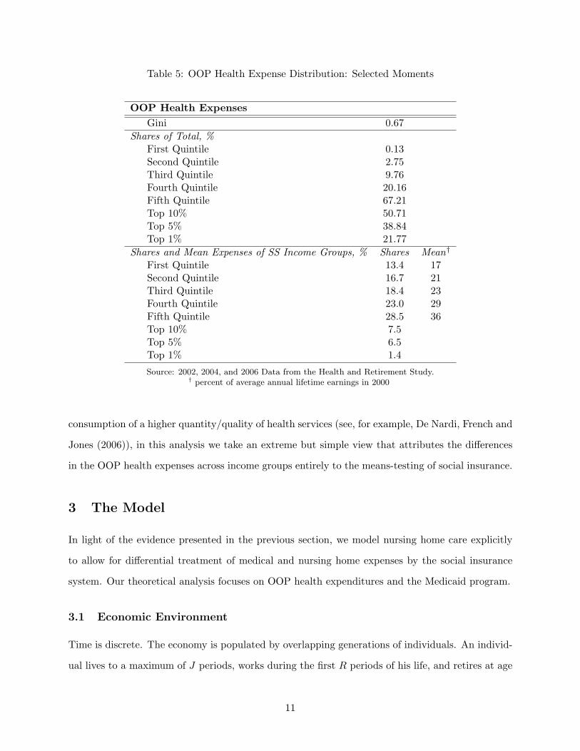
Table 3: Per Capita Private, Medicare and Medicaid Health Expenditures as a Percent of IncomePer Capita, 2002

Age Private Medicare Medicaid

65+ 12.3 17.5 5.2

65-74 9.7 12.6 2.775-84 12.7 20.9 5.285+ 21.6 27.2 15.1

Source: U.S. Department of Health and Human Services.

Table 4: Percent of Nursing Home Residents by Primary Payment Source for Individuals of AllAges and Sources of Payment for Nursing Homes/Long-term care Institutions for Individuals Ages65 and Over, 2002

Source of Payment % of NH residents ‡ % of total NH exp.‡‡ % of GDP ‡‡

Total NH exp. 100 100 0.85

Private 26 43 0.37Out-of-pocket 37 0.31

Private Insurance 2 0.02Other 4 0.04

Public 74 57 0.48Medicare 15 18 0.15Medicaid 58 37 0.31Other 1 2 0.02

‡ Source: Kaiser Commission on Medicaid and Uninsured, prepared by E. O’Brien and R. Elias, 2004‡‡ Source: Medicare Current Beneficiary Survey, 2002.

“personal needs allowance” to their nursing home and medical expenses. Although they can keep

their home and car while confined to a nursing home, these assets do not contribute much if any

to their level of consumption. In a nursing home facility, Medicaid covers room and board, nursing

care, therapy care, meals, and general medical supplies. However, Medicaid does not pay for a

single room, personal television and cable, phone and service, radios, batteries, clothes and shoes,

repairs of personal items, personal care services, among other goods and services. The result is

that the quality of life delivered to Medicaid-funded nursing home residents falls well below that of

privately-financed nursing home residents. This view is supported by survey evidence documented

by Ameriks et al. (2007) who find that wealthy people tend to avoid public long-term care due to

its low quality of life. This avoidance is termed “Medicaid aversion.”

Most estimates suggest that at age 65 the probability of ever entering a nursing home before

9

death is somewhere between 0.3 and 0.4 and the average duration of stay is approximately 2 years.

However, while the majority of entrants will spend less than 1 year in a nursing home, with very

little out-of-pocket expense risk thanks to Medicare, there is still a sizable risk of long-term stay

in a nursing home resulting in large OOP expenses. For example, Brown and Finkelstein (2008)

estimate, consistently with the findings of Dick, Garber, and MaCurdy (1994), that approximately

40 percent of entrants will spend more than 1 year in a nursing home, while approximately one

fifth will spend more than 5 years.

In our theoretical analysis, we capture the differential public insurance for nursing home versus

medical expenses by allowing for a differential in the consumption floor guaranteed under impov-

erishing medical expenses versus nursing home expenses and by calibrating the differential to be

consistent with the data on Medicaid’s share of total nursing home expenses. We show that this dif-

ferential insurance for medical versus nursing home expenses plays an important role in the saving

behavior of the wealthy.

2.3 Distribution of Out-of-Pocket Health Expenditures

To assess the cross-sectional inequality in health expenditures, we use the Health and Retirement

Survey, waves 2002, 2004 and 2006, covering medical and nursing home expense information for

the years 2000 through 2005. Our sample consists of individuals, both married and single, 65 years

of age and older. We include insurance premia in the out-of-pocket health expenditures. Table 5

presents a set of moments describing the distribution of OOP medical and nursing home expenses

for this sample.

We find that the distribution of OOP health expenses across the elderly is highly unequal, with

a Gini coefficient of 0.67 and a normalized standard deviation of 2.77. In addition, the expenses are

highly concentrated at the top of the distribution, with the top 10 percent of the elderly accounting

for more than half and the top 1 percent for more than a fifth of total OOP expenses. Moreover,

OOP expenses increase with permanent earnings. Since data on lifetime earnings is not available

to us, we use social security (SS) income as a proxy. The top SS income quintile spends OOP about

twice as much as the bottom quintile. Such a pattern is expected in the presence of a means-tested

subsidy which provides more social insurance to the lower-income quintiles. Although some studies

find that the rich spend more on health services not only due to lower subsidies, but also due to

10

Table 5: OOP Health Expense Distribution: Selected Moments

OOP Health Expenses

Gini 0.67

Shares of Total, %First Quintile 0.13Second Quintile 2.75Third Quintile 9.76Fourth Quintile 20.16Fifth Quintile 67.21Top 10% 50.71Top 5% 38.84Top 1% 21.77

Shares and Mean Expenses of SS Income Groups, % Shares Mean†

First Quintile 13.4 17Second Quintile 16.7 21Third Quintile 18.4 23Fourth Quintile 23.0 29Fifth Quintile 28.5 36Top 10% 7.5Top 5% 6.5Top 1% 1.4

Source: 2002, 2004, and 2006 Data from the Health and Retirement Study.† percent of average annual lifetime earnings in 2000

consumption of a higher quantity/quality of health services (see, for example, De Nardi, French and

Jones (2006)), in this analysis we take an extreme but simple view that attributes the differences

in the OOP health expenses across income groups entirely to the means-testing of social insurance.

3 The Model

In light of the evidence presented in the previous section, we model nursing home care explicitly

to allow for differential treatment of medical and nursing home expenses by the social insurance

system. Our theoretical analysis focuses on OOP health expenditures and the Medicaid program.

3.1 Economic Environment

Time is discrete. The economy is populated by overlapping generations of individuals. An individ-

ual lives to a maximum of J periods, works during the first R periods of his life, and retires at age

11

R + 1. While working, an individual faces uncertainty about his earnings, and starting from the

retirement age, he faces uncertainty about his survival, medical expenses, and nursing home needs.

The government runs a social insurance program that guarantees a minimum consumption level.

This consumption level differs by the type of destitution: due to low earnings of workers, or due to

impoverishing medical or nursing home expenses of the retired. In addition, the government runs

a pay-as-you-go social security program. Markets are competitive.

Individual earnings evolve over the life-cycle according to a function Ω(j, z) that maps individual

age j and current earnings shock z into efficiency units of labor, supplied to the labor market at wage

rate w. The earnings shock z follows an age-invariant Markov process with transition probabilities

given by Λzz′ . The efficiency units of the new-born workers is distributed according to a p.d.f. Γz.

Similarly, medical expenditures evolve stochastically according to a function M(j, h) that maps

individual age j and current expenditure shock h into out-of-pockets costs of health care. The

medical expenditure shock h follows an age-invariant Markov process with transition probabilities

Λhh′ . The initial distribution of medical expenditure shocks is given by Γh and it is independent

of the individual state.

The need for nursing home care in the next period of life, at age j + 1, arises with probability

θ(j+1, h) at each age j > R+1 and with probability θR+1 at age R+1. The probability of entering

a nursing home next period is increasing in age. For agents beyond age R+1 the entry probability

is increasing in the previous period’s medical expense. For simplicity, we assume that nursing home

is an absorbing state. While in a nursing home, agents have constant medical expenditure Mn,

which corresponds to the health shock value hn.

There are no insurance markets to hedge either earnings, medical expenditure, nursing home, or

mortality risks. Self-insurance is achieved with precautionary savings (labor supply is exogenous).

Individuals cannot borrow. Unintended bequests are taxed away by the government and are used

to finance government expenditure and social insurance transfers.7

7We do this to avoid the unrealistic impact that redistributing bequests as lump-sum transfers would have onagents eligibility for means-tested transfers. In addition, we wish to avoid the unrealistic impact that an arbitraryredistribution of bequests would have on individuals’ saving behavior in response to changes in the social insurancesystem.

12

3.2 Demographics

Agents face survival probabilities that are conditional on both age and nursing home status. The

probability that an age-(j − 1) individual survives to age j is sj if he is not residing in a nursing

home, and snj < sj if he is in a nursing home. Since a working-age agent faces neither mortality nor

nursing home risk, his survival probability is sj = 1, j = 1, 2, ..., R. Let θj denote the unconditional

(independent of the previous period’s medical expense) probability of entering a nursing home at

age j. Then, without conditioning on his current medical expense shock, an age-(j − 1), retired

individual enters a nursing home in period j with probability θj > 0. Let λj denote the fraction

of cohort j residing in a nursing home. This fraction is zero for working-age cohorts. For a newly

retired cohort, the fraction is just the unconditional probability of entering a nursing home, so

λR+1 = θR+1. Finally, for a retired cohort of age R + 1 < j ≤ J , the fraction λj evolves according

to

λj =θjsj(1− λj−1) + snj λj−1

sj,

where the denominator, sj = sj(1−λj−1)+ snj λj−1, is the average survival rate from age j− 1 to j

and the numerator is a weighted sum of the survival rate of new entrants and the survival rate of

current residents.

Population grows at a constant rate n. Then the size of cohort j relative to that of cohort j− 1

is

ηj =ηj−1sj1 + n

, for j = 2, 3, ..., J.

3.3 Workers’ Savings

The state of a working individual consists of his age j, assets a, average lifetime earnings to date e,

and current productivity shock z. The individual’s taxable income y consists of his interest income

ra and labor earnings e net of the payroll tax τe(e). The individual allocates his assets, taxable

income less income taxes τy(y), and transfers from the government T (j, y, a) between consumption

c and savings a′ by solving

V (j, a, e, z) = maxc,a′≥0

U(c) + βEz

[V (j + 1, a′, e′, z′)

](1)

13

subject to

c+ a′ = a+ y − τy(y) + T (y, a), (2)

y = e− τe(e) + ra, (3)

e = wΩ(j, z), (4)

e′ = (e+ je)/(j + 1), (5)

T (y, a) = max0, cw −

[a+ y − τy(y)

]. (6)

where cw is a minimum consumption level guarranteed to workers.

3.4 Old-age Health Care

Retired individuals face uncertainty about their medical and nursing home needs. The nursing

home state is entered once and for all, but every period individuals can choose between private

and public nursing home care.8 An individual’s nursing home status is denoted by the variable l,

which takes a value of either 0, indicating that the individual is currently not in a nursing home,

1, indicating that he is currently in a nursing home under private care, or 2, indicating that he is

currently in a nursing home under public care.

3.4.1 Medical care

Conditional on surviving to the next period, a working individual of age R with state (a, e, z) will

enter a nursing home upon retirement with probability θR+1. His future state contains a health

shock, h′, that determines his medical care costs. The problem of this individual is

V (R, a, e, z) = maxc,a′≥0

U(c) + βsR+1(1− θR+1)E

[V (R+ 1, a′, e, h′, 0)

]+ (7)

βsR+1θR+1max[V (R+ 1, a′, e, hn, 1), V (R+ 1, a′, e, hn, 2)

](8)

subject to the constraints above.

Resources of a retired individual of age j > R come from the return on his savings (1+ r)a, his

8The assumption that the nursing home state is absorbing is not unreasonable given that we set the model periodto two years, Dick et al. (1994) find that the majority of long-term nursing home spells end in death and Murtaughet al. (1997) find that the majority of nursing home users die within one year of discharge.

14

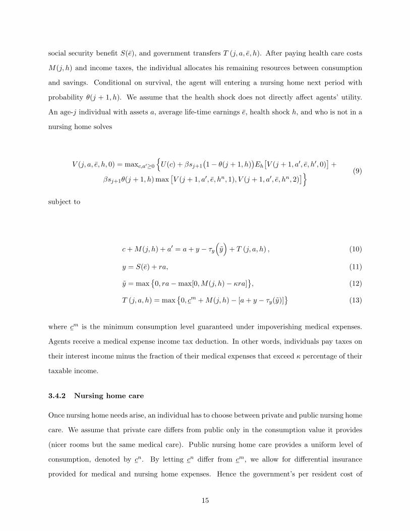
social security benefit S(e), and government transfers T (j, a, e, h). After paying health care costs

M(j, h) and income taxes, the individual allocates his remaining resources between consumption

and savings. Conditional on survival, the agent will entering a nursing home next period with

probability θ(j + 1, h). We assume that the health shock does not directly affect agents’ utility.

An age-j individual with assets a, average life-time earnings e, health shock h, and who is not in a

nursing home solves

V (j, a, e, h, 0) = maxc,a′≥0

U(c) + βsj+1

(1− θ(j + 1, h)

)Eh

[V (j + 1, a′, e, h′, 0)

]+

βsj+1θ(j + 1, h)max[V (j + 1, a′, e, hn, 1), V (j + 1, a′, e, hn, 2)

] (9)

subject to

c+M(j, h) + a′ = a+ y − τy

(y)+ T (j, a, h) , (10)

y = S(e) + ra, (11)

y = max0, ra−max[0,M(j, h)− κra]

, (12)

T (j, a, h) = max0, cm +M(j, h)− [a+ y − τy(y)]

(13)

where cm is the minimum consumption level guaranteed under impoverishing medical expenses.

Agents receive a medical expense income tax deduction. In other words, individuals pay taxes on

their interest income minus the fraction of their medical expenses that exceed κ percentage of their

taxable income.

3.4.2 Nursing home care

Once nursing home needs arise, an individual has to choose between private and public nursing home

care. We assume that private care differs from public only in the consumption value it provides

(nicer rooms but the same medical care). Public nursing home care provides a uniform level of

consumption, denoted by cn. By letting cn differ from cm, we allow for differential insurance

provided for medical and nursing home expenses. Hence the government’s per resident cost of

15

nursing home care is Mn + cn. To qualify for public nursing home care, an individual must meet

the following eligibility criteria: his income net of taxes plus the value of assets have to fall below a

threshold level. Note that individuals will only choose public care if their consumption level under

private care falls below cn. In addition, since the agents’ income streams during retirement are

deterministic and constant, an agent receiving public care would never choose to switch to private

care in the future. Thus, for simplicity, we assume that when an individual enters public care he

surrenders all of his assets as well as current and future pension income to the government and has

no further decisions to make.

An individual in private nursing home care decides how much to save and whether to switch to

public nursing care by solving

V (j, a, e, hn, 1) = maxc,a′≥0

u(c) + βsnj+1max

[V (j + 1, a′, e, hn, 1), V (j + 1, a′, e, hn, 2)

](14)

subject to

c+Mn + a′ = a+ y − τy

(max

0, ra−max[0,Mn − κra]

), (15)

y = S(e) + ra, (16)

where the value of entering a public nursing home is

V (j + 1, a′, e, hn, 2) =J∑

i=j

βi−ji−1∏k=j

snk+1u(cn)

≡ V nj+1.

Note that there are no government transfers to individuals receiving private nursing home care.

However, such individuals are still eligible for a medical expense tax deduction.

3.5 Goods Production

Firms produce goods by combining capital K and labor L according to a constant-returns-to-scale

production technology: F (K,L). Capital depreciates at rate δ and can be accumulated through

investments of goods: I = K ′ − (1 − δ)K. Firms maximize profits by renting capital and labor

from households. Perfectly competitive markets ensure that factors of production are paid their

16

marginal products. Goods can be consumed by individuals, used in health care, and invested in

physical capital.

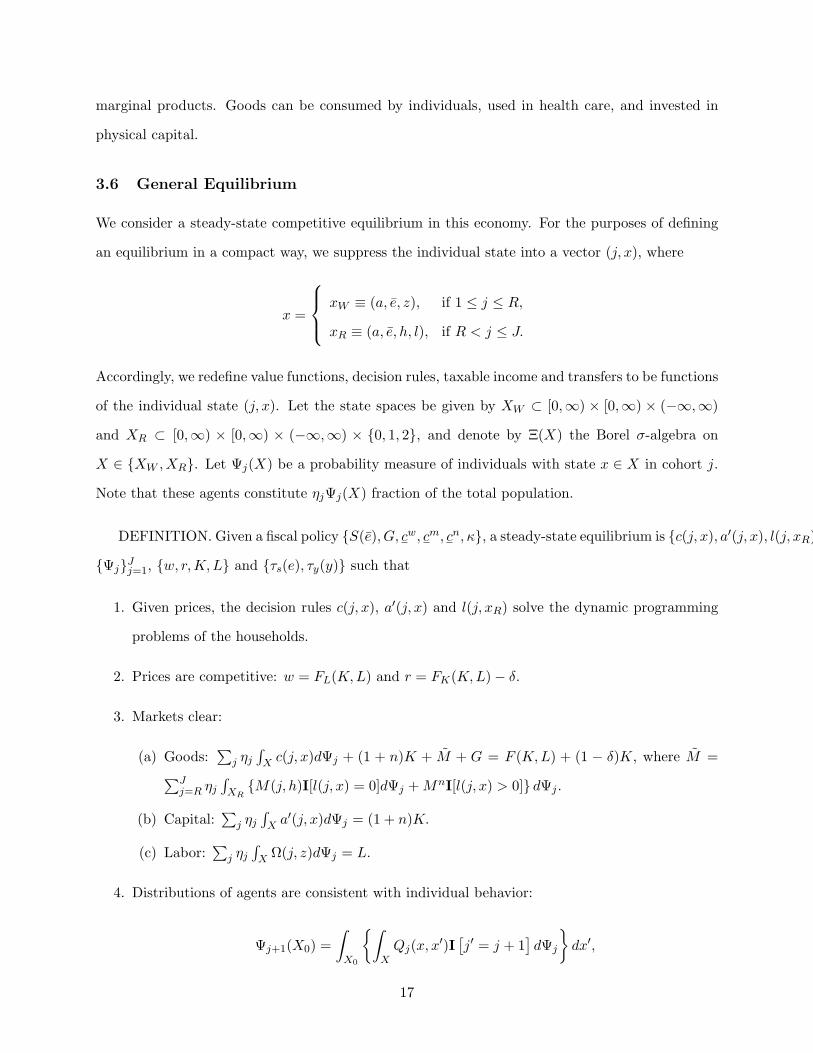
3.6 General Equilibrium

We consider a steady-state competitive equilibrium in this economy. For the purposes of defining

an equilibrium in a compact way, we suppress the individual state into a vector (j, x), where

x =

xW ≡ (a, e, z), if 1 ≤ j ≤ R,

xR ≡ (a, e, h, l), if R < j ≤ J.

Accordingly, we redefine value functions, decision rules, taxable income and transfers to be functions

of the individual state (j, x). Let the state spaces be given by XW ⊂ [0,∞) × [0,∞) × (−∞,∞)

and XR ⊂ [0,∞) × [0,∞) × (−∞,∞) × 0, 1, 2, and denote by Ξ(X) the Borel σ-algebra on

X ∈ XW , XR. Let Ψj(X) be a probability measure of individuals with state x ∈ X in cohort j.

Note that these agents constitute ηjΨj(X) fraction of the total population.

DEFINITION. Given a fiscal policy S(e), G, cw, cm, cn, κ, a steady-state equilibrium is c(j, x), a′(j, x), l(j, xR), V (j, x),

ΨjJj=1, w, r,K,L and τs(e), τy(y) such that

1. Given prices, the decision rules c(j, x), a′(j, x) and l(j, xR) solve the dynamic programming

problems of the households.

2. Prices are competitive: w = FL(K,L) and r = FK(K,L)− δ.

3. Markets clear:

(a) Goods:∑

j ηj∫X c(j, x)dΨj + (1 + n)K + M + G = F (K,L) + (1 − δ)K, where M =∑J

j=R ηj∫XR

M(j, h)I[l(j, x) = 0]dΨj +MnI[l(j, x) > 0] dΨj .

(b) Capital:∑

j ηj∫X a′(j, x)dΨj = (1 + n)K.

(c) Labor:∑

j ηj∫X Ω(j, z)dΨj = L.

4. Distributions of agents are consistent with individual behavior:

Ψj+1(X0) =

∫X0

∫XQj(x, x

′)I[j′ = j + 1

]dΨj

dx′,

17

for all X0 ∈ Ξ, where I is an indicator function and Qj(x, x′) is the probability that an agent

of age j and current state x transits to state x′ in the following period. (A formal definition

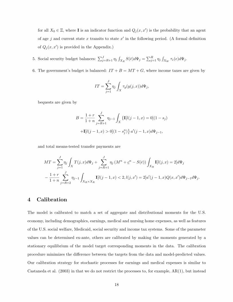
of Qj(x, x′) is provided in the Appendix.)

5. Social security budget balances:∑J

j=R+1 ηj∫XR

S(e)dΨj =∑R

j=1 ηj∫XW

τe(e)dΨj .

6. The government’s budget is balanced: IT +B = MT +G, where income taxes are given by

IT =J∑

j=1

ηj

∫Xτy(y(j, x))dΨj ,

bequests are given by

B =1 + r

1 + n

J∑j=R+1

ηj−1

∫XI[l(j − 1, x) = 0](1− sj)

+I[l(j − 1, x) > 0](1− snj )a′(j − 1, x)dΨj−1,

and total means-tested transfer payments are

MT =

J∑j=1

ηj

∫XT (j, x)dΨj +

J∑j=R+1

ηj (Mn + cn − S(e))

∫XR

I[l(j, x) = 2]dΨj

− 1 + r

1 + n

J∑j=R+2

ηj−1

∫XR×XR

I[l(j − 1, x) < 2, l(j, x′) = 2]a′(j − 1, x)Q(x, x′)dΨj−1dΨj .

4 Calibration

The model is calibrated to match a set of aggregate and distributional moments for the U.S.

economy, including demographics, earnings, medical and nursing home expenses, as well as features

of the U.S. social welfare, Medicaid, social security and income tax systems. Some of the parameter

values can be determined ex-ante, others are calibrated by making the moments generated by a

stationary equilibrium of the model target corresponding moments in the data. The calibration

procedure minimizes the difference between the targets from the data and model-predicted values.

Our calibration strategy for stochastic processes for earnings and medical expenses is similar to

Castaneda et al. (2003) in that we do not restrict the processes to, for example, AR(1), but instead

18

target a wide set of moments characterizing the earnings and OOP health expense distributions.

Unlike Castaneda et al., we do not target the distribution of wealth because part of our objective

is to learn how much wealth inequality can be generated by idiosyncratic risk in earnings, health

expenses, and survival in a pure life-cycle model. We do not restrict the stochastic processes for

earnings and medical expenses to AR(1) processes for the following reasons. First, as Castaneda et

al. (2003) demonstrate, models which use AR(1) processes for earnings have difficulty generating

the degree of earnings inequality observed in the data and, second, French and Jones (2004) find

that the the stochastic process for medical expenses is not well approximated by an AR(1) process.

Thus we choose the parameters of the discrete Markov chains for earnings and medical expenses to

match directly the earnings and medical expense distributions in the data.

We start by presenting functional forms and setting parameters whose direct estimates are

available in the data. Although the calibration procedure identifies the rest of the parameters by

solving a simultaneous set of equations, for expositional purposes, we divide the parameters to be

calibrated into groups and discuss associated targets and their measurement in the data. Most of

the data statistics used in the calibration procedure are averages over or around 2000-2006, which

is the time period covered by the HRS. More fundamental model parameters rely on long-run data

averages.

4.1 Age structure

In the model, agents are born at age 21 and can live to a maximum age of 100. We set the model

period to two years because the data on OOP health expenses is available bi-annually. Thus the

maximum life span is J = 40 periods. For the first 44 years of life, i.e. the first 22 periods, the

agents work, and at the beginning of period R+ 1 = 23, they retire.

Population growth rate n targets the ratio of population 65 year old and over to that 21 years old

and over. According to U.S. Census Bureau, this ratio was 0.18 in 2000. We target this ratio rather

than directly set the population growth rate because the weight of the retired in the population

determines the tax burden on workers, which is of a primary importance to our analysis of the

effects of the social insurance system.

19

4.2 Preferences

The momentary utility function is assumed to be of the constant-relative-risk-aversion form

U(c) =c1−γ

1− γ,

so that 1/γ is the intertemporal elasticity of substitution. Based on estimates in the literature, we

set γ equal to 2.0. The subjective discount factor, β is determined in the calibration procedure

such that the rate of return on capital in the model is consistent with an annual rate of return of

4 percent.

4.3 Technology

Consumption goods are produced according to a production function,

F (K,L) = AKαL1−α,

where capital depreciates at rate δ. The parameters α and δ are set using their direct counterparts

in the U.S data: a capital income share of 0.3 and an annual depreciation rate of 7 percent (Gomme

and Rupert (2007)). The parameter A is set such that the wage per an efficiency unit of labor is

normalized to one under the benchmark calibration .

4.4 Earnings Process

In the model, worker’s productivity depends on his age and an idiosyncratic productivity shock

according to a function Ω(j, z). We assume that this function consists of a deterministic age-

dependent component and a stochastic component as follows:

log Ω(j, z) = log∑

i∈0,1

exp[β1(j + i) + β2(j + i)2

]+ z,

where z follows a finite-valued Markov process with probability transition matrix Λzz′ . Initial

productivity levels are drawn from the distribution Γz.

The coefficients on age and age-squared are set to 0.109 and -0.001, respectively, obtained from

20

1968 to 1996 PSID data on household heads.9 We assume that there are 5 possible values for z and

that the probabilities of going from the two lowest productivity levels to the highest one and from

the two highest ones to the lowest one are 0. These restrictions, combined with a normalization

and imposing the condition that the rows of Λzz′ and elements of Γz must sum to one, leaves 24

parameters to be determined. These parameters are chosen by targeting the following statistics:

the variance of log earnings of households with heads age 55 relative to those with heads age 35, the

first-order autocorrelation of earnings, the Gini coefficient for earnings, 8 points on the Lorenz curve

for earnings, corresponding to the five quintiles and top 1, 5, and 10 percent of the distribution,

mean Social Security income levels by Social Security income quintile, and 8 points in the Lorenz

curve for Social Security income. Thus we target a relative variance for 55 year-olds of 1.89 and

a first-order autocorrelation for z of 0.97 (converted from an annual autocorrelation of 0.98) using

estimates taken from Storesletten et al. (2004). The data points for the earnings Lorenz curve are

taken from Rodriguez at el. (2002). The targets on the Lorenz curve for Social Security income and

mean Social Security by quintile are taken from waves 2002 through 2006 of the HRS. We target

mean Social Security income by quintiles since we also target mean OOP medical expenditures by

Social Security income quintiles, as discussed below. We use social security income quintiles as a

proxy for lifetime earnings quintiles because lifetime earnings is not available to us.

4.5 Medical Expense Process

Retired agents not residing in a nursing home face medical expenses that are a function of their

current age and medical expense shock. Similarly to the earnings process, we assume that medical

expenses can be decomposed into a deterministic age component and a stochastic component:

lnM(j, h) = βm,1j + βm,2j2 + h,

where h follows a finite state Markov chain with probability transition matrix Λhh′ and newly

retired agents draw their medical expense shock h from an initial distribution denoted by Γh.

We assume that for each age there are 4 possible medical expense levels, which we fix exoge-

9The sample is restricted to the heads of household, between the age of 18 and 65, not self-employed, not workingfor the government, working at least 520 hours during the year; excluding observations with the average hourly wage(computed as annual earnings over annual hours worked) less than half the minimum wage in that year; weightedusing the PSID sample weights. We thank Gueorgui Kambourov for providing us with the regression results.

21

nously. Thus specifying the process for h requires choosing 20 parameters: 16 parameters specifying

the probability transition matrix for h, Ωhh′ , and 4 parameters characterizing the initial distribution

of medical expenditure shocks, Γh. Since the rows of the transition matrix and the initial distribu-

tion must sum to one, the degrees of freedom to be determined reduces to 15. Thus, including the

coefficients in the deterministic component, 17 parameters still remain to be chosen to specify the

medical expense process.

To calibrate the 17 parameters governing the OOP health expense process, we use 20 aggregate

and distributional moments for OOP health expenses: the Gini coefficient and 8 points in the

Lorenz curve of the OOP medical expense distribution, shares of OOP health expenses and Medicaid

expenses in GDP for each age group – 65 to 74 year-olds, 75 to 84 year-olds, and those 85 and above

– and the shares of the OOP health expenses that are paid by each social security income quintile.

The targets and their values in the data are summarized in the next section. The distributional

moments were documented in section 2 using the HRS data. OOP and Medicaid expenses by age

groups are 2001-2006 averages based on the aggregate data from the U.S. Department of Health

and Human Services. Note that our measure of OOP health expenditures corresponds to the sum

of all private health care expenditures, including the costs of health insurance.

4.6 Nursing Home Expense Risk

The nursing home expense risk in the model is intended to capture the risk expenses due to a

long-term (more than one year) stay in a nursing home. Starting at age R, agents face age-specific

probabilities of entering a nursing home for a long-term stay in the following period and starting

at age R + 1, entry probabilities depend on both age and health. The unconditional probabilities

of entering a nursing home at each age j + 1 are θjJj=R+1 and the probabilities conditional on

health are θ(j+1, h)Jj=R+1. We assume that, at each age j, the probability of entering a nursing

home next period increases in M(j, h) at a constant rate or

ln θ(j + 1, h) = βjn,1 + βj

n,2 lnM(j, h), j = R+ 1, . . . , J.

For simplicity we assume that the rate at which the entry probability increases with health is

constant across ages, i.e., βjn,2 = βn,2 for all j > R. In addition, we assume that the unconditional

22

probability of entering a nursing home is the same across agents within the following age groups:

65 to 74, 75 to 84, and 85 years old and above. Thus, given βn,2, the parameters βjn,1Jj=R+1 are

chosen such that the unconditional nursing home entry probabilities satisfy

θj =

θ65−74, for 1 ≤ R+ j < 6,

θ75−84, for 6 ≤ R+ j < 11,

θ85+, for 11 ≤ R+ j ≤ J,

and the 3 probabilities, θ65−74, θ75−84, and θ85+, target the percentage of individuals residing in

a nursing home for at least one year in each age group. According to the U.S. Census special

tabulation for 2000, these percentage were 1.1, 4.7, and 18.2, respectively. The growth rate βn,2 is

chosen along with the parameters of the medical expense process by targeting Medicaid’s share of

medical expenses by age.

The medical cost of 2 years of nursing home care in the model economy, Mn targets the share

of total nursing home expenses net of those paid by Medicare in GDP. Since Medicare pays for

most of the nursing home costs for individuals with short-term stays, this share captures well the

total expenditure on long-term residents. According to statistics drawn from the Medicare Current

Beneficiary Surveys from the period 2000 to 2003, the average cost of nursing home care net of

Medicare payments was 0.68 percent of GDP. Note that to be consistent with the data, in the model,

total nursing home expenses are computed as the sum of the medical costs and consumption in a

nursing home: Mn + cn.

4.7 Survival Probabilities

Recall that while agents of age j = R + 1, . . . , J not residing in a nursing home have probability

sj+1 of surviving to age j + 1 conditional on having survived to age j, retired agents residing in

nursing homes face different survival probabilities, given by snj Jj=R+2. These two sets of survival

probabilities are not set to match their counterparts in the data for two reasons: first, there are

no estimates of survival probabilities by nursing home status available for the U.S., and second,

since we are targeting statistics on aggregate nursing home costs, it is important for the model to

be consistent with the data on nursing home usage. Therefore, the survival probabilities are set as

23

follows. First, we assume that for each cohort, the probability of surviving to the next age while

in a nursing home is a constant fraction of the probability of surviving to the next age outside of

a nursing home:

snj = ϕnsj , for j = R+ 2, . . . , J.

Then we pin-down the value of ϕn by targeting the fraction of individuals aged 65 and over residing

in nursing homes in the U.S. in 2000 subject to the restriction that the unconditional age-specific

survival probabilities are consistent with those observed in the data.10 According to U.S. Census

special tabulation for 2000, the fraction of the 65 plus population in a nursing home in 2000 was

4.5 percent.

4.8 Government

The government-run welfare program in the model economy guarantees agents a minimum consump-

tion level. The welfare program, which is available to all agents regardless of age, represents public

assistance programs in the U.S. such as food stamps, Aid to Families with Dependent Children,

Supplemental Social Security Income, and Medicaid. Since estimates of the government-guaranteed

consumption levels for working versus retired individuals are found to be very similar, we assume

that they are the same. However, the level of social insurance of destitution due to high health

expenses depends on the type of expenses – nursing home or medical. In the literature, estimates

of the consumption level for a family consisting of one adult and two children is approximately 35

percent of expected average annual lifetime earnings, while the minimum level for retired house-

holds has been estimated to be in the range of 15 to 20 percent (Hubbard, Skinner, and Zeldes

(1994) and Scholz, Seshadri, and Khitatrakun (2006)).11 These estimates suggest that the mini-

mum consumption floor for individuals is somewhere in the range of 10 to 20 percent.12 We set the

10The data on survival probabilities is taken from Table 7 of Life Tables for the United States Social Security Area1900-2100 Actuarial Study No. 116 and are weighted averages of the probabilities for both men and women born in1950.

11Expected average annual lifetime earnings in 1999 is computed as a weighted average of estimates of averagelifetime earnings for different education groups taken from The Big Payoff: Educational Attainment and SyntheticEstimates of Work-Life Earnings. U.S. Census Bureau Special Studies. July 2002. The weights are taken fromEducational Attainment: 2000 Census Brief. August 2003.

12However, this statement should be taken with caution. The consumption floor is difficult to measure due tothe large variation and complexity in welfare programs and their coverage. In addition, families with two adultsand adults under 65 without children would receive substantially less in benefits then found above. Consistent withthis, by estimating their model, DeNardi, French, and Jones (2006), find a much lower minimum consumption level:approximately 8 percent of expected average annual lifetime earnings. This is similar to a value of about 6 percent

24

consumption floor for workers and retirees not in a nursing home, cw = cm, to 15 percent of the

average annual earnings.

Obtaining an estimate of a consumption floor provided to nursing home residents is problematic

because it requires estimating the value of the rooms and amenities that nursing homes provide to

Medicaid-funded residents. Instead, we calibrate the minimum consumption level for nursing home

residents, cn, to match Medicaid’s share of nursing home expenses for individuals 65 and over.

According to the Current Medicare Beneficiary Survey, over the period 2000 to 2003, on average,

Medicaid’s share of the elderly’s total nursing home expenses net of those paid by Medicare was

approximately 45 percent.

The social security benefit function in the model captures the progressivity of the U.S. social

security system by making the marginal replacement rate decrease with average earnings. Following

Fuster, Imrohoroglu, and Imrohoroglu (2006), the marginal tax replacement rate is 90 percent for

earnings below 20 percent of the economy’s average earnings E, 33 percent for earnings above that

threshold but below 125 percent of E, and 15 percent for earnings beyond that up to 246 percent

of E. There is no replacement for earnings beyond 246 percent of E. Hence the payment function

is

S(e) =

s1e, for e ≤ τ1,

s1τ1 + s2(e− τ1), for τ1 ≤ e ≤ τ2,

s1τ1 + s2(τ2 − τ1) + s3(e− τ2), for τ2 ≤ e ≤ τ3,

s1τ1 + s2(τ2 − τ1) + s3(τ3 − τ2), for e ≥ τ3.

where the marginal replacement rates, s1, s2, and s3 are set to 0.90, 0.33, and 0.15, respectively.

While the threshold levels, τ1, τ2, and τ3, are set respectively to 20 percent, 125 percent and 246

percent of the economy’s average earnings.

The payroll tax which is used to fund the social security system is assumed to be proportional,

thus

τe(e) = τee,

where the tax rate τe is determined in equilibrium. Likewise, income taxes in the model economy

used by Palumbo (1999). However, health expenses in the model of DeNardi et al. include nursing home costs, andhence their estimate is not directly comparable to the non-nursing home minimum consumption level in our model.Thus we do not use their estimate.

25

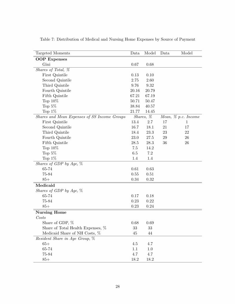
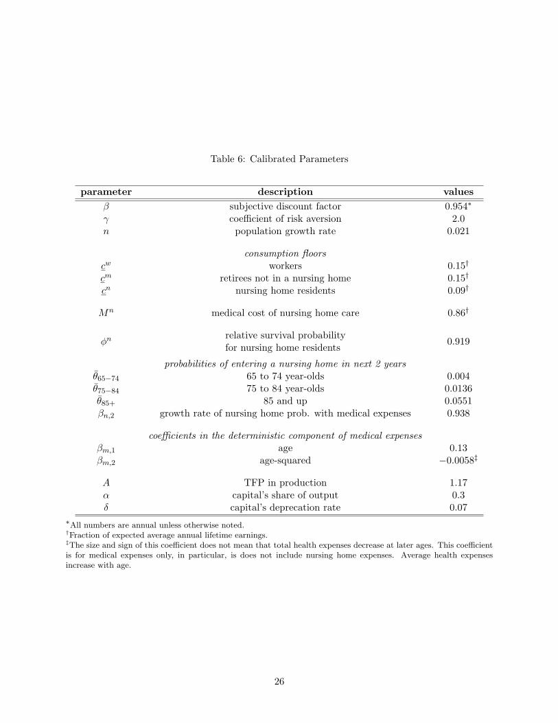
Table 6: Calibrated Parameters

parameter description values

β subjective discount factor 0.954∗

γ coefficient of risk aversion 2.0n population growth rate 0.021

consumption floorscw workers 0.15†

cm retirees not in a nursing home 0.15†

cn nursing home residents 0.09†

Mn medical cost of nursing home care 0.86†

ϕn relative survival probabilityfor nursing home residents

0.919

probabilities of entering a nursing home in next 2 yearsθ65−74 65 to 74 year-olds 0.004θ75−84 75 to 84 year-olds 0.0136θ85+ 85 and up 0.0551βn,2 growth rate of nursing home prob. with medical expenses 0.938

coefficients in the deterministic component of medical expensesβm,1 age 0.13βm,2 age-squared −0.0058‡

A TFP in production 1.17α capital’s share of output 0.3δ capital’s deprecation rate 0.07

∗All numbers are annual unless otherwise noted.†Fraction of expected average annual lifetime earnings.‡The size and sign of this coefficient does not mean that total health expenses decrease at later ages. This coefficientis for medical expenses only, in particular, is does not include nursing home expenses. Average health expensesincrease with age.

26

are assumed to be proportional so that

τy(y) = τyy.

The tax rate τy is also determined in equilibrium. As is the case under the U.S. tax system, taxable

income is income net of health expenses that exceed 7.5 percent of income. Thus κ is set to 0.075.

Finally, government spending, G is set such that, in equilibrium, government spending as a fraction

of output is 19 percent.

4.9 Benchmark calibration

The model parametrization is summarized in Table 6. Information on the algorithm used to com-

pute the equilibrium along with the transition probability matrices and other parameters governing

the earnings and OOP health expense processes are included in the Appendix. The equilibrium

tax rates in the benchmark economy are 0.254 for income tax and 0.079 for payroll tax. Note that

our calibration produced a value for the nursing home consumption floor, cn, which lies below the

non-nursing home consumption floor, cm. We view this differential as reflecting a lower quality of

life enjoyed in a public nursing home facility relative to receiving public assistance while living at

home. As we show later in our quantitative analysis, the low quality of life under public nursing

care plays an important role in individual saving decisions.

The exogeneity of the earnings distribution allows us to match it with a much greater precision

then other sources of heterogeneity in the model economy. Since the contribution of our analysis

comes from modeling medical and nursing home expense risk, we confine our discussion to the

latter, while reporting the fit of the earnings distribution in the Appendix.

In the data, individual medical expenses are only observed net of public subsidies. Hence we

calibrate the stochastic process for total medical and nursing home expenses to match aggregate

levels of OOP health expenses and their observed distribution across the population. In particular,

we target the cross-sectional distribution of OOP expenses, shares of OOP and Medicaid expenses

in GDP by age group, and the distribution of OOP expenses by social security income. Moreover,

the nursing home expense process targets the distribution of nursing home residents and aggregate

nursing home costs by source of payment. The results of the calibration procedure are presented

27

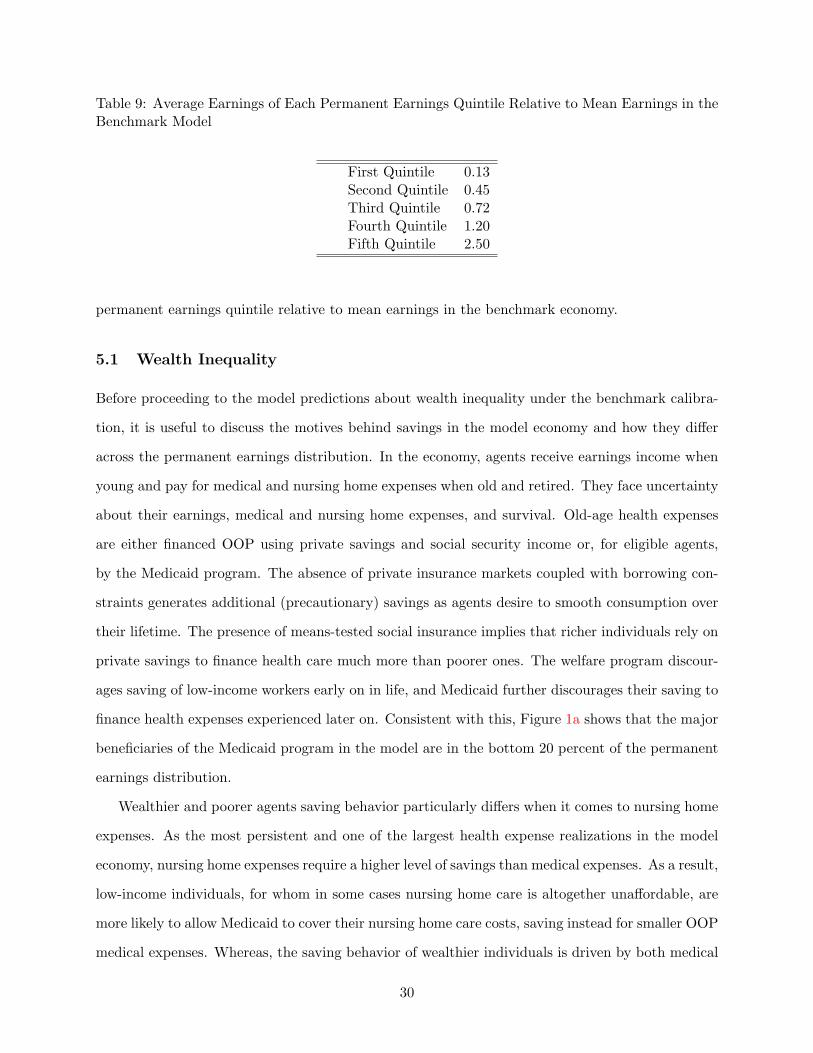
Table 7: Distribution of Medical and Nursing Home Expenses by Source of Payment

Targeted Moments Data Model Data Model

OOP ExpensesGini 0.67 0.68

Shares of Total, %First Quintile 0.13 0.10Second Quintile 2.75 2.60Third Quintile 9.76 9.32Fourth Quintile 20.16 20.79Fifth Quintile 67.21 67.19Top 10% 50.71 50.47Top 5% 38.84 40.57Top 1% 21.77 14.45

Shares and Mean Expenses of SS Income Groups Shares, % Mean, % p.c. IncomeFirst Quintile 13.4 2.7 17 1Second Quintile 16.7 18.1 21 17Third Quintile 18.4 23.3 23 22Fourth Quintile 23.0 27.5 29 26Fifth Quintile 28.5 28.3 36 26Top 10% 7.5 14.2Top 5% 6.5 7.2Top 1% 1.4 1.4

Shares of GDP by Age, %65-74 0.61 0.6375-84 0.55 0.5185+ 0.34 0.32

MedicaidShares of GDP by Age, %

65-74 0.17 0.1875-84 0.23 0.2285+ 0.23 0.24

Nursing HomeCosts

Share of GDP, % 0.68 0.69Share of Total Health Expenses, % 33 33Medicaid Share of NH Costs, % 45 44

Resident Share in Age Group, %65+ 4.5 4.765-74 1.1 1.075-84 4.7 4.785+ 18.2 18.2

28

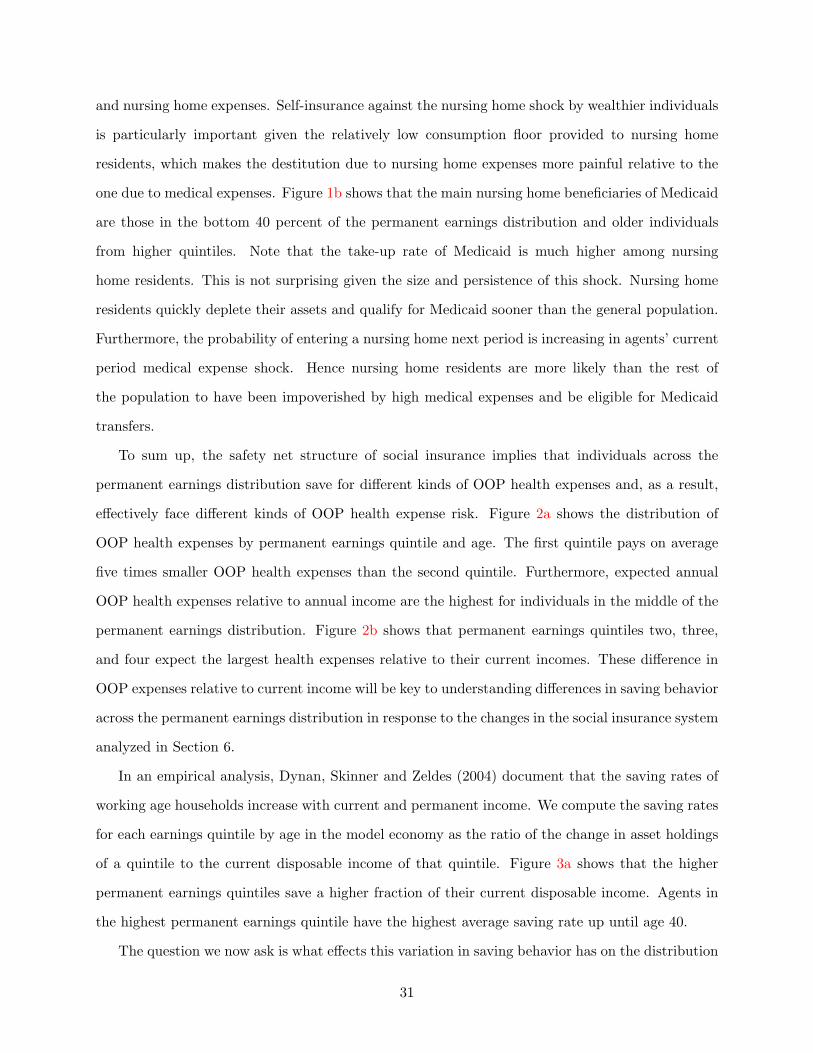
Table 8: Medical and Nursing Home Expenses: Aggregate Summary

Health Expense Data Model

MedicalOOP, % of GDP 1.5 1.5Medicaid, % of GDP 0.6 0.6

Nursing HomeOOP, % of GDP, % 0.38 0.39Medicaid, % of GDP 0.31 0.30

Independent MomentsFraction of NH residents on Medicaid 0.58∗ 0.60Nursing Home Entry Probability 0.14† 0.15∗ includes individuals under 65† probability of entering and staying a year or more

in Table 7. Overall, the distribution of OOP health expenses in the benchmark economy closely

replicates a wide range of data moments. Table 8 summarizes the cross-sectional targets from Table

7 into aggregate statistics for the benchmark economy, showing a good model fit with the data on

aggregate. Among the independent moments characterizing health expenses, the model successfully

predicts the fraction of nursing home residents receiving Medicaid subsidy and the probability of

entering a nursing home for a long-term stay.

5 The Benchmark Economy

In this section we first assess the ability of the calibrated model to generate cross-sectional and

life-cycle wealth inequality as observed in the U.S. economy. We then examine the contribution

of precautionary savings to wealth accumulation and inequality. Building a life-cycle theory of

economic inequality is crucial for a quantitative analysis of the impact of health expenses and the

structure of old-age social insurance on savings and inequality for many reasons. To name a few,

first, social safety nets target the low-income population. Second, the savings response to various

types of risks may differ across the permanent earnings distribution. Finally, when wealth is highly

concentrated in the hands of a few, their saving behavior has large consequences for the whole

economy. In order to assess how individuals vary across the permanent earnings distribution, we

often compare individuals across permanent earnings quintiles. Table 9 shows the earnings of each

29

Table 9: Average Earnings of Each Permanent Earnings Quintile Relative to Mean Earnings in theBenchmark Model

First Quintile 0.13Second Quintile 0.45Third Quintile 0.72Fourth Quintile 1.20Fifth Quintile 2.50

permanent earnings quintile relative to mean earnings in the benchmark economy.

5.1 Wealth Inequality

Before proceeding to the model predictions about wealth inequality under the benchmark calibra-

tion, it is useful to discuss the motives behind savings in the model economy and how they differ

across the permanent earnings distribution. In the economy, agents receive earnings income when

young and pay for medical and nursing home expenses when old and retired. They face uncertainty

about their earnings, medical and nursing home expenses, and survival. Old-age health expenses

are either financed OOP using private savings and social security income or, for eligible agents,

by the Medicaid program. The absence of private insurance markets coupled with borrowing con-

straints generates additional (precautionary) savings as agents desire to smooth consumption over

their lifetime. The presence of means-tested social insurance implies that richer individuals rely on

private savings to finance health care much more than poorer ones. The welfare program discour-

ages saving of low-income workers early on in life, and Medicaid further discourages their saving to

finance health expenses experienced later on. Consistent with this, Figure 1a shows that the major

beneficiaries of the Medicaid program in the model are in the bottom 20 percent of the permanent

earnings distribution.

Wealthier and poorer agents saving behavior particularly differs when it comes to nursing home

expenses. As the most persistent and one of the largest health expense realizations in the model

economy, nursing home expenses require a higher level of savings than medical expenses. As a result,

low-income individuals, for whom in some cases nursing home care is altogether unaffordable, are

more likely to allow Medicaid to cover their nursing home care costs, saving instead for smaller OOP

medical expenses. Whereas, the saving behavior of wealthier individuals is driven by both medical

30

and nursing home expenses. Self-insurance against the nursing home shock by wealthier individuals

is particularly important given the relatively low consumption floor provided to nursing home

residents, which makes the destitution due to nursing home expenses more painful relative to the

one due to medical expenses. Figure 1b shows that the main nursing home beneficiaries of Medicaid

are those in the bottom 40 percent of the permanent earnings distribution and older individuals

from higher quintiles. Note that the take-up rate of Medicaid is much higher among nursing

home residents. This is not surprising given the size and persistence of this shock. Nursing home

residents quickly deplete their assets and qualify for Medicaid sooner than the general population.

Furthermore, the probability of entering a nursing home next period is increasing in agents’ current

period medical expense shock. Hence nursing home residents are more likely than the rest of

the population to have been impoverished by high medical expenses and be eligible for Medicaid

transfers.

To sum up, the safety net structure of social insurance implies that individuals across the

permanent earnings distribution save for different kinds of OOP health expenses and, as a result,

effectively face different kinds of OOP health expense risk. Figure 2a shows the distribution of

OOP health expenses by permanent earnings quintile and age. The first quintile pays on average

five times smaller OOP health expenses than the second quintile. Furthermore, expected annual

OOP health expenses relative to annual income are the highest for individuals in the middle of the

permanent earnings distribution. Figure 2b shows that permanent earnings quintiles two, three,

and four expect the largest health expenses relative to their current incomes. These difference in

OOP expenses relative to current income will be key to understanding differences in saving behavior

across the permanent earnings distribution in response to the changes in the social insurance system

analyzed in Section 6.

In an empirical analysis, Dynan, Skinner and Zeldes (2004) document that the saving rates of

working age households increase with current and permanent income. We compute the saving rates

for each earnings quintile by age in the model economy as the ratio of the change in asset holdings

of a quintile to the current disposable income of that quintile. Figure 3a shows that the higher

permanent earnings quintiles save a higher fraction of their current disposable income. Agents in

the highest permanent earnings quintile have the highest average saving rate up until age 40.

The question we now ask is what effects this variation in saving behavior has on the distribution

31

of wealth in the economy. First, we compare the wealth inequality generated by the model to the

data. Recall that our calibration procedure did not target any wealth distribution moments. Table

10 reveals that cross-sectional wealth inequality in the benchmark economy has a remarkable fit of

the U.S. wealth distribution, as documented in Rodriguez et al. (2002). The share of wealth held

by the top 1 percent of the population in the model economy, 28 percent, is remarkably high for

a pure overlapping-generations model. Moreover, the wealth Gini in the benchmark economy is

U-shaped over the life-cycle (Figure 3b), which is consistent with the pattern observed in the data

(Huggett, 1996).

To investigate the role that health expenses and social safety nets play in generating the high

concentration of wealth in the benchmark economy, we conduct the following partial equilibrium

analysis. We first remove all health expenses from the economy. We find that not only are health ex-

penses not responsible for the high wealth concentration, but they actually reduce wealth inequality

and concentration. We then almost completely remove the safety nets from the benchmark econ-

omy by setting the consumption floors for all government transfers to a very small number. The

wealth Gini coefficient decreases by 23 percentage points and the share of wealth held by the top

1 percent falls by a half. Finally, we remove both health expenses and safety nets and compare it

to the economy without safety nets. Again, we find that health expenses reduce wealth inequality

and concentration, while the presence of safety nets dampens their effect. Thus, we conclude that

the high degree of inequality and concentration of wealth in the benchmark economy is driven by

the presence of safety nets. The findings are summarized in Table 10. In Section 6, we study these

effects in more detail and provide an explanation for the puzzling effect that health expenses have

on inequality.

5.2 Precautionary Savings Due to Old-Age Uncertainty

To further understand the drivers of saving behavior in our benchmark economy we now ask how

much of savings is precautionary savings due to uncertainty about health expenses and survival.

First, to evaluate the role of health expense risk, in a partial equilibrium, we shut down uncertainty

about all health expenses by making each retired individual face a deterministic health expense

profile regardless of their nursing home status. The expense profile is set to the average profile before

Medicaid subsidies in the benchmark economy. Note that uncertainty about health expenses due to

32

Table 10: Wealth: Selected Moments

Data Benchmark No OOP No OOPNo Safety Nets No Safety Nets

Wealth†

Gini 0.80 0.83 0.86 0.57 0.64Shares of Total, %

First Quintile -0.3 0 0 0.7 0.7Second Quintile 1.3 0 0 5.0 4.5Third Quintile 5.0 1.0 0.5 12.8 10.4Fourth Quintile 12.2 12.9 10.5 25.6 19.0Fifth Quintile 81.7 86.0 89.0 55.8 65.5Top 10% 69.1 66.8 72.4 37.5 50.0Top 5% 57.8 51.7 59.0 26.7 39.1Top 1% 34.7 28.0 33.9 13.4 21.9

† Data source: Rodriguez et al. (2002).

random survival still remains. Consistently with De Nardi et al. (2006) and Hubbard et al. (1994),

we find that, on aggregate, health expense risk plays a modest role: precautionary savings account

for 4 percent of the total capital stock (Table 11). However, the importance of health expense risk

varies over the permanent earnings distribution. In particular, it plays a more prominent role for

the fourth and fifth permanent earnings quintiles, accounting for 8 and 5 percent of their wealth,

respectively. The aggregate effect is smaller because individuals in the lower quintiles accumulate

more wealth with deterministic health expenses as they are less likely to qualify for Medicaid

subsidies in the absence of large shocks.

Notice, however, that although all quintiles face higher OOP health expenses due to a lower

Medicaid subsidy (for which they qualify with certainty after some age), their OOP nursing home

expenses drop. To disentangle the contribution of nursing home expense risk from that of medical

expense risk, we consider an economy where every retired individual faces certain medical expenses

but their nursing home expense risk is the same as in the benchmark. We find that uncertainty

about medical expenses alone accounts for only 1 percent of aggregate capital accumulation, driven

by the savings of the top two quintiles (second column in Table 11). We conclude that uncertainty

about nursing home expenses is a more important motive for precautionary savings than uncertainty

about medical expenses. The intuition behind this novel result is simple: the nursing home shock

is the most persistent shock, one of the largest health cost realizations in the model economy, and

33

the least insured by the government. These three features make nursing home expenses more risky

than medical expenses.

To assess the contribution of precautionary savings due to survival risk, we consider certain

lifetimes conditional on nursing home status. That is, since nursing home entry is random, and it

lowers the entrant’s life expectancy, survival risk due to nursing home entry still remains. We set

the lifetime horizon of an individual who never enters a nursing home equal to the life-expectancy

of the same individual in the benchmark economy. Individuals who enter nursing homes live to an

age given by the life expectancy conditional on entering a nursing home at age 65 in the benchmark

economy. Entering a nursing home after that age is equivalent to an immediate death.

We find that survival risk plays a much more prominent role in savings than does health expense

risk. Precautionary savings due to survival risk accounts for 15 percent of the capital stock in the

benchmark economy (third column in Table 11). Why is survival risk so important for savings given

that social security already partially insures individuals against this type of risk? This happens

for two reasons. First, social security income is insufficient for consumption smoothing of richer

individuals, and second, the presence of health expenses and their growth with age make surviving

increase lifetime health expense risk. Means-testing of Medicaid makes this risk more important for

wealthier individuals. As Table 11 shows, deterministic survival leads to a decrease in the wealth of

the top three permanent earnings quintiles. Notice, however, that part of the fall in these quintiles’

wealth is due to a decline in their OOP health expenses. This decline occurs because no one lives

to ages beyond life expectancy – when health expenses are, on average, the highest.

How much do health expenses matter for the importance of survival risk? To this end, we

repeat the above experiment in an economy identical to the benchmark except with all health

expenses removed. The change in the aggregate wealth is reported in the last column in Table

11. Without health expenses, precautionary savings due to survival risk only account for 5 percent

of the aggregate capital stock. Moreover, precautionary savings are only accumulated by the top

permanent earnings quintile; the rest of the population gets enough insurance from the social

security system. We thus conclude that, although health expense risk conditional on survival

generates little precautionary savings, the presence of health expenses substantially amplifies the

role of survival risk in individual wealth accumulation. This is another novel result in the literature.

To sum up, we have shown that the benchmark economy has the following features:

34

Table 11: Effects of Old-Age Uncertainty

Health Expenses Deterministic Det. except NH Random NoneSurvival Random Random Deterministic Deterministic

relative to benchmarkrelative to random survivaland no health expenses

Agg. Capital 0.961 0.989 0.847 0.948

Wealth of PE quintilesFirst Quintile 1.09 1.06 1.04 1.06Second Quintile 1.16 1.07 1.00 1.07Third Quintile 1.04 1.00 0.89 1.02Fourth Quintile 0.92 0.97 0.81 0.99Fifth Quintile 0.95 0.99 0.88 0.95

OOP expenses of PE quintilesFirst Quintile 1.24 1.20 0.99Second Quintile 1.33 1.19 1.03Third Quintile 1.21 1.06 0.98Fourth Quintile 1.04 1.01 0.89Fifth Quintile 1.01 1.00 0.88

Nursing home OOP expenses of PE quintilesFirst Quintile 0.95 1.03 0.42Second Quintile 0.77 1.09 0.49Third Quintile 0.53 1.06 0.46Fourth Quintile 0.34 1.02 0.38Fifth Quintile 0.31 1.00 0.36

35

1. OOP health expenses increase with permanent earnings due to means-tested social insurance.

2. Relative to income, OOP health expense risk is highest for middle-income agents.

3. Wealth inequality is driven by the presence of social safety nets.

4. Uncertainty about health expenses plays a modest role in aggregate wealth accumulation.

5. Uncertainty about nursing home expenses is more important than uncertainty about medical

expenses.

6. Precautionary savings for survival risk is a significant component of aggregate savings due

to the presence of health expenses that increase with age.

Noting these features of the benchmark economy will aid in our analysis of the impact of health

expenses and the structure of the old-age social insurance system on savings and inequality, which

is the main goal of this paper and the focus of the next section.

6 The Role of Health Expenses and Social Insurance

Relative to most developed countries, the U.S. social insurance system is unique in its lack of

public health care. Instead, the elderly rely on means-tested Medicaid to avoid destitution due

to high OOP health expenses. In this section, we assess the implications of the lack of public

health care for aggregate capital accumulation and inequality in wealth and consumption. To this

end, we introduce public health care such that medical and/or nursing home expenses are fully

covered by the government. We then examine the interaction of public health care with other

social insurance programs: welfare for workers, Medicaid and old-age welfare, and social security.

All the experiments considered below are revenue-neutral in a sense that government consumption

remains fixed at the benchmark level. As these experiments are not actual policy reforms, we focus

on steady states and do not consider transition dynamics induced by changes in the social insurance

system.

Before proceeding to the experiments, we would like to clarify our terminology. It is important

to remember that Medicaid transfers to nursing home residents combine consumption and medical

expense subsidies, up to cn+Mn in the benchmark economy. When we refer to the public coverage

of nursing home expenses, or equivalently, elimination of nursing home expenses, we mean only

the medical expense portion, Mn, of the nursing home cost. Unlike under Medicaid, this subsidy

36

is provided to all nursing home residents, and it does not restrict their consumption to cn. Con-

sumption transfers to nursing home residents are subject to means-testing in all economies that we

consider below, including those with public coverage of nursing home care.

6.1 Public Health Care

To analyze the impact that limited public coverage of both medical and nursing home expenses

together and in isolation has, we consider three public health care experiments: (1) government

covers all medical expenses but does not cover nursing home expenses, (2) government covers

nursing home expenses only, (3) government covers all health expenses. In the first experiment,

social insurance for nursing home residents is unchanged, while the medical expenses of the rest

of the population are paid by the government. In the second experiment, the government pays

for the medical expenses of all nursing home residents regardless of their income, while the social

insurance coverage of all other health expenses is as in the benchmark economy. Finally, in the

third experiment both medical and nursing home expenses are paid for by the government. In

all the economies consumption transfers are subject to the same means tests as in the benchmark

economy. Aggregate and distributional effects of each experiment are reported in Table 12.

6.1.1 Aggregate Effects

Public health care greatly reduces saving incentives. Our model predicts that the aggregate capital

stock is 12 percent lower in the economy when health care is fully public (experiment 3). To show

the importance of the general equilibrium analysis, we repeat the same experiment in a partial

equilibrium. We find that changes in after-tax prices – specifically an increase in the after-tax

interest rate – offset the decline in the capital stock by 7 percentage points.

To understand which health expenses − medical or nursing home − drive the impact of public

health care on capital accumulation, we compare the effects of experiments 1 and 2, which make

publicly-provided one type of care at a time. We find that in a general equilibrium, on aggregate,

both types of expenses contribute equally: public coverage of either non-nursing home expenses only

or nursing home expenses only reduces the capital stock by 7.5 percent relative to the benchmark.

In a partial equilibrium, public coverage of nursing home expenses has a larger effect than that of

medical expenses, reducing the capital stock by 10 percent compared to 7.6 percent for medical

37

expenses. The relative importance of the lack of public coverage of nursing home care for capital

accumulation may seem surprising given that OOP nursing home expenses share of total OOP

health expenses is only 20 percent (see Table 8). However, this occurs for two reasons. First, as we

have shown in Section 5.2, because nursing home expenses are riskier than medical expenses, they

play a larger role in precautionary savings. Second, as discussed below, nursing home expenses

have a bigger impact on the savings of the top two permanent earnings quintiles. As Table 12

shows, in absolute terms, the asset holdings of these two quintiles decline the most across all three

experiments, accounting for the majority of the drop in the aggregate capital stock.

6.1.2 Distributional Effects

To examine the effects of public health care on wealth inequality, we compute percentage changes

in each permanent earnings quintile’s wealth relative to the benchmark. We find that, when all

expenses are covered by the government, asset holdings of agents in the middle of the permanent

earnings distribution – quintiles two to four – respond the most. As Table 12 indicates, these

quintiles reduce their wealth by 20 percent whereas the wealth of the first quintile is unaffected

and the top quintile reduces its wealth by only 8 percent. Moreover, comparing the changes in the

wealth holdings of each quintile relative to the benchmark under experiments 1 and 2 reveals that

nursing home expenses have a bigger impact than medical expenses on the saving behavior of the

top two permanent earnings quintiles, and the reverse is true for the second and third quintiles.

These differences in saving responses to the introduction of public health care are consistent with

the findings and intuition in the previous section: that is, because of the nature of nursing home

expenses and the structure of the social insurance system, different earnings quintiles save for

different kinds of OOP expenses, and hence respond the most to the elimination of their particular

expenses. Furthermore, between the two quintiles most exposed to the nursing home expense risk,

the fourth quintile reduces its wealth by a higher fraction than does the fifth quintile. This occurs

because, relative to their lifetime earnings, the fourth quintile’s OOP nursing home expenses are

larger.

Figure 4 plots the wealth profiles of the fourth quintile under alternative public health care

experiments. Notice that public health care discourages individual savings well before retirement.

Although before retirement savings respond similarly to public coverage of medical or nursing home

38

Table 12: Effects of Public Health Care

Experiment Benchmark 1 2 3

Medical Expenses OOP Public OOP PublicNursing Home Expenses OOP OOP Public Public

Aggregatesrelative to benchmarkAgg. Output 1.00 0.977 0.977 0.962Agg. Consumption 1.00 0.992 1.004 1.023Agg. Capital 1.00 0.925 0.925 0.878Capital, Partial Equil. 0.924 0.902 0.810change in wealth of PE quintiles, % of agg. capital changeAll 100 100 100First Quintile 0.7 -0.1 0.0Second Quintile 13.2 -0.3 6.0Third Quintile 21.7 7.6 15.3Fourth Quintile 26.8 37.9 35.0Fifth Quintile 36.0 49.6 39.6wealth of PE quintiles relative to benchmarkFirst Quintile 1.00 0.87 1.02 1.00Second Quintile 1.00 0.72 1.01 0.80Third Quintile 1.00 0.82 0.94 0.80Fourth Quintile 1.00 0.91 0.87 0.80Fifth Quintile 1.00 0.96 0.94 0.92

Income Tax Rate 0.254 0.271 0.259 0.257% of 65+ w/Transfers 23 18 21 16Health Expenses relative to benchmarkOOP 1.00 0.27 0.77 0.04†

Std(OOP) 1.00 0.74 0.73 0.10

InequalityConsumption Gini 0.417 0.424 0.426 0.434Wealth Gini 0.829 0.840 0.832 0.842shares of total wealth, %Fourth Quintile 12.9 11.5 13.1 11.9Fifth Quintile 86.1 87.7 85.8 87.2Top 10% 66.8 68.9 67.9 69.8Top 5% 51.7 54.0 53.8 56.0Top 1% 28.0 30.0 30.0 31.7

† OOP expenses are positive because, to make our measure of nursing home expenses more consistent with the

measure used in the data, we include a consumption component that is not covered in experiments 1-3.

39

expenses, the rate of dissaving up to age 85 is substantially lower when the only OOP expenses

are the ones for nursing homes. We conclude that it is the nursing home and not medical expenses

that slow down wealth depletion after retirement.

Finally, we find that the introduction of public health care – public coverage of nursing home

expenses in particular – dramatically increases inequality among retired individuals (Figure 5a),

in spite of having only a small positive effect on overall cross-sectional inequality. At the end

of the life cycle, the wealth Gini coefficient (within cohort) increases by as much as 20 points.

Higher inequality without OOP health expenses would appear rather surprising had we not already

discussed the differential response of savings to the public coverage of health expenses across the

permanent earnings quintiles. As the top quintile experiences a smaller drop in its wealth relative

to the second, third, and fourth quintiles, its share of aggregate wealth is bound to rise. Notice that

the presence of OOP medical expenses is the main driver of reduced within-cohort wealth inequality

among individuals under age 83 when going from full public health care to the benchmark, while

OOP nursing home expenses account for this reduction for the older generations. This is explained

by the fact that nursing home risk grows substantially with age: under the benchmark calibration,

the probability of entering a nursing home after age 85 is more than triple the probability for ages

75 to 84. Moreover, while we find that public health care slightly increases consumption inequality,

it substantially reduces consumption inequality among those 85 years and older (Figure 5b). These

are the people most likely to enter a nursing home and it is the coverage of nursing home expenses

that drives the fall in their consumption inequality.

The above experiments have shown that

1. Lack of public health care greatly stimulates capital accumulation;

2. OOP nursing home expenses account for half of the aggregate effect;

3. Nursing home expenses are a larger component of the savings of the rich than medical

expenses and the reverse is true for the poor;

4. The savings response to public health care differs dramatically across the permanent earnings

distribution;

5. While having a small effect on aggregate inequality, public health care significantly increases

within-cohort wealth inequality and reduces within-cohort consumption inequality among

the very old (ages above life expectancy).

40

6.2 Health Care Interaction With Other Social Insurance Programs

To what extent are these results driven by the presence of other social insurance programs? We ask

this question for the following reasons. First, recall that Medicaid provides a differential insurance

against medical versus nursing home expenses. Second, means-testing implies that rich and poor

face different types of OOP health expenses. Third, in Section 5.1, we found that wealth inequality

is driven by the presence of the safety nets (welfare and Medicaid). Fourth, both Medicaid and

pay-as-you-go social insurance partially insure the elderly against survival and health expense risk.

To understand the interactions between these social insurance programs and their implications for

the effects of public health care, we modify/eliminate one feature of the social insurance system at

a time and then compare the effects of public health care in the alternative economies to those in

the benchmark.

6.2.1 Medicaid Insurance of Nursing Home Expenses

To understand why nursing home expenses play such an important role in capital accumulation, we

modify the Medicaid means-testing so that it does not discriminate between health expenses, i.e.

it guarantees the same consumption floor to nursing home residents as the rest of the population

receives in the benchmark economy: cn = cm. We term this ‘quality’ nursing home care. We

repeat experiments (1) through (3) in the economy with quality nursing home care. The results

are presented in Table 13.

Quality public nursing home care reduces ‘Medicaid aversion’, i.e. incentives to avoid public care.

Precautionary savings fall and the capital stock declines by 4 percent relative to the benchmark

economy. Next, we introduce public health care into the economy with quality nursing home care.

Elimination of OOP health expenses in this economy reduces the capital stock by 9 percent, which is

3 percentage points less than the effect of public health care in the benchmark economy. Moreover,

quality pubic nursing home care reduces the importance of nursing home expenses relative to

medical expenses for aggregate savings. In the benchmark economy, half of the additional savings

accumulated without public health care was due to the presence of OOP nursing home expenses,

with quality nursing home care this fraction is reduced to one third. That is, a higher level of

public insurance for nursing home expenses makes this type of destitution less painful, reducing

41

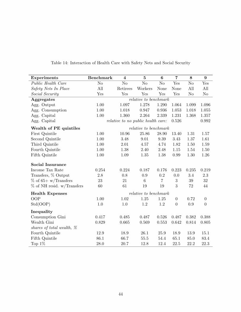
Table 13: Interaction of Nursing Home Insurance by Medicaid and Public Health Care

Experiment Benchmark Quality NH 1(Q) 2(Q) 3(Q)

Medical Expenses OOP OOP Public OOP PublicNursing Home Expenses OOP (Q)OOP (Q)OOP (Q)Public (Q)Public

AggregatesRelative to BenchmarkAgg. Output 1.00 0.988 0.965 0.977 0.962Agg. Capital 1.00 0.962 0.887 0.925 0.877Relative to Quality NHAgg. Capital 1.00 0.922 0.961 0.912

Income Tax Rate 0.254 0.259 0.277 0.260 0.257% of 65+ w/Transfers 23 23 19 21 16

Health Expenses relative to benchmarkOOP 1.00 0.99 0.26 0.80 0.07Std(OOP) 1.00 0.99 0.73 0.74 0.16

the desire to avoid it with self-insurance. Note that nursing home expenses still play a large role

in aggregate savings relative to their size – they are only one fifth of total health expenses. This is

because even with quality nursing home care, nursing home expenses are risky relative to medical

expenses due to their size and persistence. The relative impacts of health expenses on savings

are also illustrated in Figure 6 which shows the wealth profiles of the fourth permanent earnings

quintile in different experiments. Comparing with Figure 4, with quality nursing homes, the wealth

profile under publicly-funded nursing home care lies significantly closer to the profile without the

coverage. We conclude that differential insurance for nursing home care versus medical care has a

significant impact on wealth accumulation.

6.2.2 Safety Nets

We now examine the interaction of safety nets with the effects of public health care. In our model

economy, the welfare program for workers and Medicaid/welfare for retirees partially insure against

earnings, survival, and health expense risks by providing means-tested transfers that guarantee

a minimum consumption level. As means-tested welfare transfers effectively tax away low-level

savings, they discourage savings disproportionably more for the poor, reducing aggregate capital

accumulation and increasing wealth inequality (the latter shown in Section 5.1). To start, we assess

42

the role of safety nets for workers, for retirees, and for both by removing (almost completely) each

type of welfare (experiments 4 − 6). This is achieved by setting consumption floors for workers

and/or retirees to a very small value, while leaving all other features of the benchmark economy

unchanged. Then, to evaluate the contribution of safety nets to the effects of public health care, we

introduce public health care into the economy without safety nets (experiment 7). The aggregate

and distributional effects of experiments 4 through 7 are presented in Table 14.

In all the economies we consider here, agents are still partially insured through the progressive

social security program against all three types of risk. Apart from this insurance, experiment 4

maximizes individual exposure to earnings risk by removing the welfare program for workers, exper-

iment 5 maximizes individual exposure to health expense and survival risk by removing Medicaid

and the old-age welfare program, and experiment 6 maximizes individual exposure to all three types

of risks by removing all the welfare and Medicaid programs. Extra risk and higher expected OOP

health expenses create strong incentives to save across all income levels. In the economy with the

least amount of insurance (experiment 6), the capital stock increases by 134 percent. The removal

of which safety nets – those for workers or the elderly – is responsible for the large increase in

aggregate savings under experiment 6? Experiments 4 and 5 provide the answer: while removing

the welfare program for workers (experiment 4) increases the capital stock by 36 percent, remov-

ing the welfare program for the elderly (experiment 5) increases the capital stock by 126 percent.

Hence, increasing agents’ exposure to health expense risk substantially increases savings relative to

increasing their exposure to earnings risk.

Why is increased exposure to health expense risk a more important driver of precautionary sav-

ings than that for earnings risk? The answer lies in the timing of the two types of shocks. Individuals

accumulate savings during the working stages of live in order finance health expenses experienced

after retirement. These savings provide a nearly sufficient buffer against earnings shocks before

retirement. That is, consumption smoothing over the working stage of life in response to increased

earnings risk requires relatively little extra savings given the presence of OOP health expenses.

This would not have been the case were the two types of shocks experienced simultaneously.

Given the large insurance role of safety nets, it is not surprising that the introduction of public

health care into economy 6 substantially cuts down aggregate savings (by nearly a half, see experi-

ment 7) and increases wealth Gini by 9 percentage points. We conclude that the presence of safety

43

Table 14: Interaction of Health Care with Safety Nets and Social Security

Experiments Benchmark 4 5 6 7 8 9

Public Health Care No No No No Yes No YesSafety Nets In Place All Retirees Workers None None All AllSocial Security Yes Yes Yes Yes Yes No No

Aggregates relative to benchmarkAgg. Output 1.00 1.097 1.278 1.290 1.064 1.099 1.096Agg. Consumption 1.00 1.018 0.947 0.936 1.053 1.018 1.055Agg. Capital 1.00 1.360 2.264 2.339 1.231 1.368 1.357Agg. Capital relative to no public health care: 0.526 0.992

Wealth of PE quintiles relative to benchmarkFirst Quintile 1.00 10.96 25.86 28.90 13.40 1.31 1.57Second Quintile 1.00 3.48 9.01 9.39 3.43 1.37 1.61Third Quintile 1.00 2.01 4.57 4.74 1.82 1.50 1.59Fourth Quintile 1.00 1.38 2.40 2.48 1.15 1.54 1.50Fifth Quintile 1.00 1.09 1.35 1.38 0.99 1.30 1.26

Social InsuranceIncome Tax Rate 0.254 0.224 0.187 0.176 0.223 0.235 0.219Transfers, % Output 2.8 0.8 0.9 0.2 0.0 3.4 2.3% of 65+ w/Transfers 23 21 6 7 3 39 32% of NH resid. w/Transfers 60 61 19 19 3 72 44

Health Expenses relative to benchmarkOOP 1.00 1.02 1.25 1.25 0 0.72 0Std(OOP) 1.0 1.0 1.2 1.2 0 0.9 0

InequalityConsumption Gini 0.417 0.485 0.487 0.526 0.487 0.382 0.388Wealth Gini 0.829 0.665 0.569 0.553 0.642 0.814 0.805shares of total wealth, %Fourth Quintile 12.9 18.9 26.1 25.9 18.9 13.9 15.1Fifth Quintile 86.1 66.7 55.5 54.4 65.1 85.0 83.4Top 1% 28.0 20.7 12.8 12.4 22.5 22.2 22.3

44

nets for the elderly weakens the effects of public health care on wealth accumulation and inequality.

6.2.3 Social Security

The last part of the social insurance system we examine is the pay-as-you-go Social Security pro-

gram. Removing Social Security in experiment 8 causes a large (37 percent) increase in savings

for retirement and OOP health expenses. In contrast to all other economies considered above, the

introduction of public health care in such an economy has little effect on aggregate wealth accumu-

lation and inequality. Aggregate savings are nearly unaffected because savings of the bottom three

permanent earnings quintiles actually increase in response to public health care, counteracting the

decline in savings of the top two quintiles. In the economy without Social Security or public health

care (experiment 8), all individuals save for retirement, but only the wealthy also save for health

expenses. In fact, 39 percent of retirees receive means-tested transfers, so at least 39 percent of

individuals face a negative marginal return on savings. Introducing public health care lifts the

poor off the safety nets enough that they face a positive return on savings. In turn, the higher tax

base and lower transfer payments allow the government to finance public health care with a lower

income tax rate, further encouraging savings.

6.3 Discussion

To sum up, we find that there are important interactions between public health care and other

features of a social insurance system. The results of experiments in Table 14 shed some light

on how variations in social insurance systems – means-testing in particular – matter not only for

aggregate savings and consumption but also for wealth and consumption inequality. For example,

while an economy with public health care and means-tested transfers features a high degree of

wealth inequality (experiment 3), same economy without means-tested transfers has significantly

less wealth inequality and a substantially higher capital stock and consumption (experiment 7).

While our primary goal is to understand the implications of the lack of public health care for

the elderly in the U.S., these results suggest that our framework is useful for thinking about cross-

country differences in social insurance systems and their implications for savings and economic

inequality. While social insurance systems in countries like the U.S., UK, Australia, and New

Zealand target the poor through extensive means-testing, countries of continental Europe feature

45

generous universal family benefits with little use of safety nets. Furthermore, despite the fact

that most developed countries have public health care, there are large differences across countries

in public coverage of nursing home care costs and its means-testing. The number of countries

providing universal nursing home care coverage has been growing and include Austria, Germany,

Japan, Luxemburg, and the Netherlands. However, nursing home care in France, Israel, and New

Zealand is still provided through means-tested social insurance.

Moreover, countries differ in their total expenditure on nursing home care as well as in the

fraction of these expenditures which are made OOP. Among the OECD countries, in 2000, expen-

diture on nursing home care varied from 0.3 percent of GDP in France to 2.3 percent of GDP in

the Netherlands. Even within the group of countries with a universal long-term care system (no

means-testing for either home or institutional care), there is a substantial variation in the private

costs due to different beneficiary cost-sharing requirements.13 Our analysis suggests that these

differences should manifest themselves in countries’ savings and economic inequality, giving a nice

ground for a formal policy analysis. Financing the growing costs of nursing home care, and long-

term care in general, has become a key concern for policymakers as well as individuals in ageing

societies around the world. According to the OECD report on long-term care by Fujisawa and

Colombo (2009), in the past decade, real per capita long-term nursing care spending has increased

by an average of 6.5 percent per year across 24 OECD countries. In 16 OECD countries, per capita

private expenses on long-term nursing care have on average tripled between 2000 and 2006.

7 Conclusions

Our analysis has shown that lack of public health care for the elderly plays a big role in wealth

accumulation but that the aggregate and distributional effects depend on the availability of other

programs comprising the social insurance system, such as social safety nets for young and old and

pay-as-you-go social security. Here we would like to reemphasize a couple of novel results. First, we

found that social insurance of nursing home care plays a special role in wealth accumulation. The

lack of public coverage of nursing home care costs greatly stimulates wealth accumulation by richer

individuals and promotes consumption inequality among the elderly. This effect is in part due to

13These expenses may include food, housing, and other copayments; these may be related to income.

46

the lower level of insurance provided by Medicaid for nursing home care relative to that for medical

care. Second, we found that the relationships between the extent and type of social insurance and

various economic indicators are complex and highly dependent on the eligibility criteria – universal

versus means-tested – to receive social assistance from a particular government program.

In order to make our results transparent, we simplified our analysis by abstracting from endo-

geneity of labor supply, differential mortality, utility derived from health and care, the household’s

life-cycle, caregiving and other transfers within the family. Abstraction from labor supply decisions

means we have not taken into account distortions caused by the labor income tax and social safety

nets as well as self-insurance through an intertemporal substitution in labor in response to earnings

shocks. Since in the data life expectancy is higher for high-income individuals, the lifetime health

expense risk faced by these individuals is also higher, which may enhance the differential effects of

social insurance policies we found in our study. Our calibration strategy exploits the assumption

that the positive relationship observed between individual permanent income and OOP health ex-

penses (De Nardi et al. (2006)) is completely accounted for by the presence of safety nets. That

is, richer individuals face higher OOP expenses due to the means-testing of Medicaid transfers.

However, it would be interesting to relax this assumption by incorporating a choice of health care

quality and study how this margin responds to policy changes. We also assumed that health shocks

carry no disutility. While the evidence is mixed, lower marginal utility of consumption at older

ages, especially for nursing home residents, would imply that individuals put a smaller weight on

bad health states and hence require smaller savings for old age.

Extending the model by incorporating the household life-cycle – marriage, divorce, spousal

death, and children – would allow additional and potentially important dimensions to be considered.

For example the importance of differential health expense risk and mortality for men and women

and for married individuals versus singles could be assessed. Marriages may be important because

nursing home risk potentially differs by martial status, in part, because risk-sharing is available

within a household.14 Since a large fraction of lifetime health expenses are experienced in the last

year of life, often impoverishing the surviving spouse, the risk of spousal death and the extent to

which survivor benefits provided by the social insurance system insure this risk may be important for

14Heterogeneity in health and demand for nursing care open yet another avenue for modeling bargaining withinthe household.

47

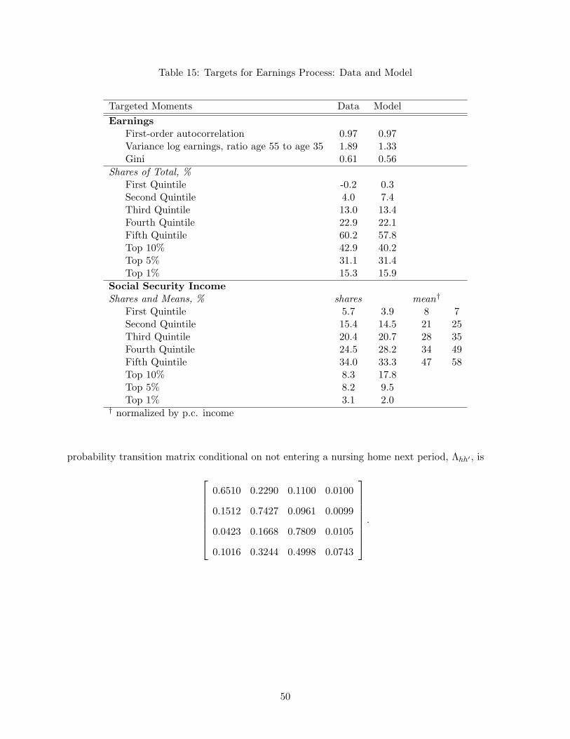
individual savings decisions. A household approach would also allow one to endogenize caregiving

decisions within the family and nursing home entry. In the data, institutional care satisfies only

a small part of long-term care needs. The majority of the elderly with needs receive their care

informally from family members – mostly spouses and children – while some obtain formal in-home

nursing care. Moreover, an intergenerational set-up would allow one to examine the exchange of

wealth and care time between parents and children. As government programs in many countries

use subsidies to encourage home care – a less costly alternative to institutional care, it would be

interesting to examine the caregiver’s labor supply response to such policies. We leave these issues

for future research.

Appendix

A.1 Probability Transition Matrix

Formally, the probability of an age-j agent going from current state x to future state x′ is given by

Qj(x, x′) ≡ I

[j = 1, a′ = a′(1, a, 0, z), e′ = wΩ(1, z)

]Γz

+ I[1 ≤ j < R, a′ = a′(j, a, e, z), e′ = (wΩ(j, z) + je)/(j + 1)

]Λz,z′

+ I[j = R, a′ = a′(R, a, e, z), e′ = e

]×

Γh′I

[l′ = 0

](1− θR+1) + I

[h′ = hn, l′ > 0

]θR+1

+ I

[R < j ≤ J, a′ = a′(j, a, e, h, 0), e′ = e

]×

Λh,h′I

[l′ = 0

](1− θ(j + 1, h)) + I

[h′ = hn, l′ = 1

]θ(j + 1, h)

sj+1

sj+1

+ I[R < j ≤ J, a′ = a′(j, a, e, hn, 1), e′ = e, l′ = 1

] snj+1

sj+1

+ I[R < j ≤ J, a′ = 0, e′ = e, l′ = 2

] snj+1

sj+1.

A.2 Computation

The steps in computing the model equilibrium are as follows. First guesses on aggregate capital

and the income tax rate are made. Note that the social security tax rate can be computed ex ante.

Second, individual maximization problems are solved. Agents’ problems in the last period of their

48

lives are solved first, followed by the previous period, up to the first period. Individual decision

rules are computed using piecewise linear interpolation. The grids for assets and average lifetime

earnings consist of 200 and 100 nonlinearly-spaced points, respectively. Third, the distribution

of the population over the discrete state is computed using forward iteration. Finally, updated

aggregates are computed. This procedure is iterated on until the capital stock converges and the

government budget constraint holds.

A.3 Earnings Process

The stochastic component of the earnings process consists of a five-state discrete Markov chain. The

chain is characterized by a five element grid of possible realizations, an initial distribution over that

grid, Γz, and a 25 element probability transition matrix, Λzz′ . The grid, which is set such that ex-

pected average annual earnings in the model is normalized to one, is [−6.4823, 0.0155, 0.8747, 1.2000, 3.2102].

The initial distribution, probability transition matrix and grid are chosen by minimizing the dif-

ference between the model’s prediction and the data on the 24 statistics mentioned in Section

4.3. The minimization results are provided in Table 15. The initial distribution generated by the

minimization is [0.0552, 0.5270, 0.2578, 0.1300, 0.0300] and the probability transition matrix is

0.9684 0.0267 0.0049 0.0000 0

0.0424 0.9305 0.0271 0.0000 0

0.0079 0.0229 0.9682 0.0010 0.0000

0 0.0052 0.0635 0.9300 0.0013

0 0.0104 0.0198 0.0200 0.9497

.

A.4 Medical Expense Process

The stochastic component of the medical expense process is governed by a four-point discrete

Markov chain. Its grid of realizations is [−5.83,−3.00,−1.70, 0.685], the initial distribution of

non-nursing home entrants across medical expenses, Γh, is [0.2205, 0.2177, 0.5209, 0.0409], and the

49

Table 15: Targets for Earnings Process: Data and Model

Targeted Moments Data Model

EarningsFirst-order autocorrelation 0.97 0.97Variance log earnings, ratio age 55 to age 35 1.89 1.33Gini 0.61 0.56

Shares of Total, %First Quintile -0.2 0.3Second Quintile 4.0 7.4Third Quintile 13.0 13.4Fourth Quintile 22.9 22.1Fifth Quintile 60.2 57.8Top 10% 42.9 40.2Top 5% 31.1 31.4Top 1% 15.3 15.9

Social Security IncomeShares and Means, % shares mean†

First Quintile 5.7 3.9 8 7Second Quintile 15.4 14.5 21 25Third Quintile 20.4 20.7 28 35Fourth Quintile 24.5 28.2 34 49Fifth Quintile 34.0 33.3 47 58Top 10% 8.3 17.8Top 5% 8.2 9.5Top 1% 3.1 2.0

† normalized by p.c. income

probability transition matrix conditional on not entering a nursing home next period, Λhh′ , is

0.6510 0.2290 0.1100 0.0100

0.1512 0.7427 0.0961 0.0099

0.0423 0.1668 0.7809 0.0105

0.1016 0.3244 0.4998 0.0743

.

50

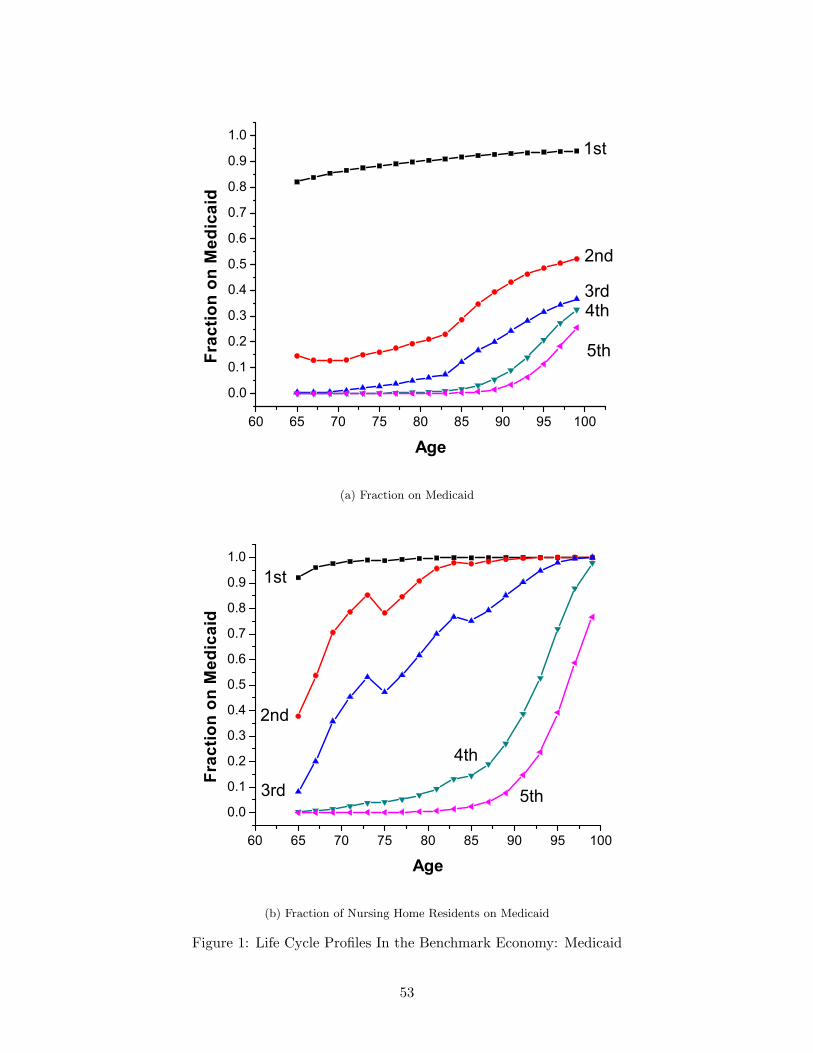
References

[1] Ameriks, J, A. Caplin, S. Laufer, S. Van Nieuwerburgh (2007). “The Joy of Giving or AssitedLiving? Using Strategic Surveys to Separate Bequest and Precautionary Motives.” NBERWorking Paper 13105.

[2] Attanasio, O, S. Kitao, G. L. Violante (2008). “Financing Medicare: A General EquilibriumAnalysis.” Forthcoming in J. B. Shoven, ed., Topics in Demography and the Economy (NBER).

[3] Brown, J. and A. Finkelstein (2008). “The Interaction of Public and Private Insurance: Med-icaid and the Long-Term Care Insurance Market.” American Economic Review, vol. 98, no. 3,pp: 1083-1102.

[4] Castaneda, A., J. Diaz-Gimenez, J.V. Rios-Rull (2003). “Accounting for the U.S. Earningsand Wealth Inequality,” Journal of Political Economy, vol. 111, no. 4, pp: 818-857.

[5] Dick, A., A. Garber, and T. MaCurdy (1994) “Forecasting Nursing Home Utilization of ElderlyAmericans.” In David Wise (ed.) Studies in the Economics of Aging.

[6] De Nardi, M., E. French, J. B. Jones (2006). “ Differential Mortality, Uncertain MedicalExpenses, and the Saving of the Elderly Singles,” mimeo.

[7] Dynan, K., J. Skinner and S. P. Zeldes (2004). “Do the Rich Save More?” Journal of PoliticalEconomy, vol. 112, no. 2, pp: 397-444.

[8] French, E. and J. B. Jones (2003). “The Effects of Health Insurance and Self-Insurance onRetirement Behavior,” mimeo.

[9] French, E., and J. B. Jones (2004). “On the Distribution and Dynamics of Health Care Costs,”Journal of Applied Econometrics, vol. 19, no. 4, pp: 705-721.

[10] Fuster, L. (1999). “Is Altruism Important for Understanding The Long Run Effects of SocialSecurity?,” Review of Economic Dynamics, vol. 2, no. 3, pp: 616-637.

[11] Fuster, L., A. Imrohoroglu and S. Imrohoroglu (2006). “Elimination of Social Security in aDynastic Framework,” forthcoming, Review of Economic Studies.

[12] Gertler, P., and J. Gruber (2006). “Insuring Consumption Against Illness,” American Eco-nomic Review, vol. 92, no. 1, pp: 51-69.

[13] Gomme, P. and P. Rupert (2007). “Theory, Measurement and Calibration of MacroeconomicModels,” Journal of Monetary Economics, vol. 54, no. 2, pp: 460-497.

[14] Hubbard, G.R., J. Skinner, and S. Zeldes (1994). “The Importance of Precautionary Motivesin Explaining Individual and Aggregate Saving,” Carnegie-Rochester Conference Series onPublic Policy, vol. 40, pp: 59-125.

[15] Hubbard, G.R., J. Skinner, and S. Zeldes (1995). “Precautionary Savings and Social Insur-ance,” Journal of Political Economy, vol. 103, no. 2, pp: 360-399.

[16] Huggett, M. (1996). “Wealth Distribution in Life-Cycle Economies,” Journal of MonetaryEconomics, vol. 38, pp: 469-494.

51

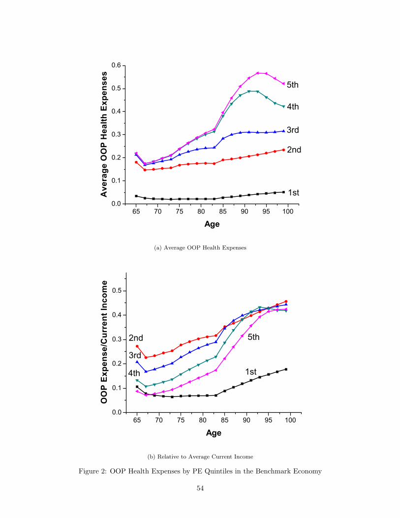
[17] Kotlikoff, L. J. (1988). “Health Expenditures and Precautionary Savings.” In L. J. Kotlikoff,ed., What Determines Savings? MIT Press.

[18] Mollica, R.L. (2009). “State Medicaid Reimbursement Policies and Practices in Assisted Liv-ing,” Prepared for: National Center for Assisted Living, American Health Care Association.

[19] Murtaugh, C.M., P. Kemper, B.C. Spillman, B. Lepidus Carlson (1997). “The Amount, Distri-bution, and Timing of Lifetime Nursing Home Use,” Medical Care, vol. 35, no. 3, pp: 204-218.

[20] Palumbo, M.G. (1999). “Uncertain Medical Expenses and Precautionary Saving Near The Endof Life Cycle,” Review of Economic Studies, vol. 66, pp: 395-421.

[21] Rodriguez, S. B., J. Diaz-Gimenez, V. Quadrini, J.-V. Rios-Rull (2002). “Updated Facts onthe U.S. Distributions of Earnings, Income and Wealth,” Federal Reserve Bank of MinneapolisQuarterly Review, vol. 26, no. 3, pp: 2-25.

[22] Scholz, J.K., A. Seshadri, S. Khitatrakun (2006). “Are Americans Saving Optimally for Re-tirement?” Journal of Political Economy, vol. 114, no. 4, pp:607-643.

[23] Storesletten, K., C. Telmer, and A. Yaron (2004). “Consumption and Risk Sharing Over theLife Cycle,” Journal of Monetary Economics, vol. 51, pp: 609-633.

52

60 65 70 75 80 85 90 95 100

0.0

0.1

0.2

0.3

0.4

0.5

0.6

0.7

0.8

0.9

1.0

2nd

3rd

5th

4th

Frac

tion

on M

edic

aid

Age

1st

(a) Fraction on Medicaid

60 65 70 75 80 85 90 95 100

0.0

0.1

0.2

0.3

0.4

0.5

0.6

0.7

0.8

0.9

1.0

5th

4th

3rd

2nd

1st

Frac

tion

on M

edic

aid

Age

(b) Fraction of Nursing Home Residents on Medicaid

Figure 1: Life Cycle Profiles In the Benchmark Economy: Medicaid

53

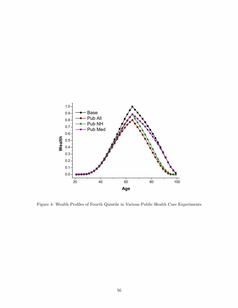
65 70 75 80 85 90 95 1000.0

0.1

0.2

0.3

0.4

0.5

0.6

1st

2nd

3rd

4th

5th

Ave

rage

OO

P H

ealth

Exp

ense

s

Age

(a) Average OOP Health Expenses

65 70 75 80 85 90 95 1000.0

0.1

0.2

0.3

0.4

0.5

4th

2nd

3rd

5th

1st

OO

P Ex

pens

e/C

urre

nt In

com

e

Age

(b) Relative to Average Current Income

Figure 2: OOP Health Expenses by PE Quintiles in the Benchmark Economy

54

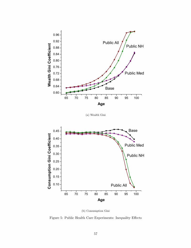
20 40 60 80 100

-0.8

-0.6

-0.4

-0.2

0.0

0.2

0.4

5th

4th

3rd2nd

1stA

vera

ge S

avin

g R

ate

Age

(a) Saving Rates

20 40 60 80 100

0.2

0.3

0.4

0.5

0.6

0.7

0.8

0.9

1.0

Consumption

Wealth

Gin

i Coe

ffici

ent

Age

Earnings

(b) Gini Coefficients

Figure 3: Life Cycle Profiles In the Benchmark Economy: Inequality

55

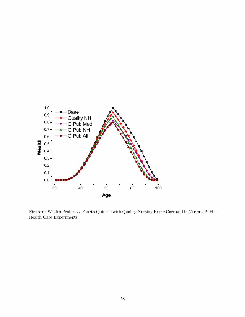
20 40 60 80 100

0.0

0.1

0.2

0.3

0.4

0.5

0.6

0.7

0.8

0.9

1.0

Wea

lth

Age

Base Pub All Pub NH Pub Med

Figure 4: Wealth Profiles of Fourth Quintile in Various Public Health Care Experiments

56

65 70 75 80 85 90 95 100

0.60

0.64

0.68

0.72

0.76

0.80

0.84

0.88

0.92

0.96

Public AllPublic NH

Base

Public Med

Wea

lth G

ini C

oeffi

cien

t

Age

(a) Wealth Gini

65 70 75 80 85 90 95 100

0.10

0.15

0.20

0.25

0.30

0.35

0.40

0.45

Public All

Public NH

Base

Public Med

Con

sum

ptio

n G

ini C

oeffi

cien

t

Age

(b) Consumption Gini

Figure 5: Public Health Care Experiments: Inequality Effects

57

20 40 60 80 100

0.0

0.1

0.2

0.3

0.4

0.5

0.6

0.7

0.8

0.9

1.0

Wea

lth

Age

Base Quality NH Q Pub Med Q Pub NH Q Pub All

Figure 6: Wealth Profiles of Fourth Quintile with Quality Nursing Home Care and in Various PublicHealth Care Experiments

58