The Impact of New Urbanism on Single Family Housing Values:

The Case of Issaquah Highlands

Jinyhup Kim

A thesis

submitted in partial fulfillment of the

requirements for the degree of

Master of Urban Planning

University of Washington

2015

Committee:

C.-H. Christine Bae

Christopher Bitter

Program Authorized to Offer Degree:

College of Built Environments

ⓒCopyright 2015

Jinyhup Kim

University of Washington

Abstract

The Impact of New Urbanism on Single Family Housing Values:

The Case of Issaquah Highlands

Jinyhup Kim

Chair of the Supervisory Committee:

Professor C.-H. Christine Bae

Department of Urban Design and Planning

New Urbanism has been a prevalent issue in architecture and planning fields over the last few

decades as an alternative to reforming the sprawl pattern of suburban growth. New Urbanist

design principles have been adopted for many housing and neighborhood planning efforts in the

United States. Do the attributes of New Urbanism serve as an impetus for improving economic

value through increasing property value?

This study compares Issaquah Highlands’ home prices with those of traditional suburban single

family homes in the City of Issaquah. The null hypothesis is that consumers are willing to pay

similar prices for houses in Issaquah Highlands and for houses in the surrounding conventional

subdivisions. The principal database used consists of US Census Washington State Geospatial

Data Archive (WAGDA), and the King County Tax Assessments. The final data set consists of

1,075 single family housings over the three-year period from 2012 to 2014 based on sale records

throughout the City of Issaquah. This study uses the hedonic pricing technique to assess the

impact of New Urbanism on the value of single family residences through linear and semi-log

functional form.

Descriptive statistics show that more expensive properties are located in Issaquah Highlands

($638,358), followed by All Sales ($622,066), and Out of Issaquah Highlands ($608,673). 45.1

percent of sampled properties are in Issaquah highlands, and 54.9 percent are outside of Issaquah

Highlands.

The findings suggest that a binary variable representing New Urbanism indicates that people are

willing to pay a $40,985-$56,762 premium (approximately 6.2-6.5 percent) for houses in

Issaquah Highlands. The present study is valuable to urban planners, developers, and policy

makers by providing several implications for future research and policy development in the

urban planning field.

i

Table of Contents

Pages

List of Tables...………………………………………………….………………………………..iii

List of Figures...…………………………………………………..………………………………iv

Chapter 1 Introduction….….…………………………………….....……………………………..1

1.1 Background……………….……………………………...…..……………………………1

1.2 Purpose of Thesis…….…………………………………...……..………………………...5

1.3 Thesis Structure……….…...……………………………...….…………………………...7

Chapter 2 Literature Review….…….……………………………...…..………………………….9

2.1 New Urbanism Principles…….…………………………...……..………………………10

2.2 New Urbanism’s Impact on Property Value……...………...…….………………………13

2.3 Other Factors Impacting Property Value.…….…...………...………….………………...15

2.4 Hypotheses………….………………...………...………...………..…………………….22

Chapter 3 The Case of Issaquah Highlands….….……..………...……….……………………...23

3.1 Regional Context…..……………….…………………...……….………………………23

3.2 Community Guiding Principles..…………..…………….………………………………25

Chapter 4 Data…….…...…….……..………………………………….…………...……………31

4.1 Data Sources..…..……….……………………………………..…………...……………32

4.2 Data Selection…..….…………………………………………..…………...……………34

4.3 Quantitative Measures of Data for Neighborhood Analysis…….….……………………36

4.4 Summary of Variables…..…….…………...……………………..………………………40

ii

Chapter 5 Methodology….……....………...…………………………….………………………45

5.1 Research Design...………………...…………….………………..………………………45

5.2 Research Method………………...…………...........…………….………………………47

Chapter 6 Result…….….………………...………………………………..……………………..51

6.1 T-Test Independent Samples..….....……………..………………….……………………51

6.2 Descriptive Statistics…………...……………….…………………..……………………52

6.3 Hedonic Pricing Model and Results.……..……..……………….………………………55

6.4 Discussion……..……………………..………….…………………..………………...…66

Chapter 7 Conclusion……….………………………………………………..…………………..68

References.…..……...……………….………….…………………………..…………………..70

Appendix.….…………………..…….………….…………………………..…………………..73

iii

List of Tables

Pages

Table 1 Summary of major studies on property impact of built environment reviewed……...…20

Table 2 Lists of GIS data sets used….……....………………………………..………..………...32

Table 3 List of Tax assessments data sets used……………………………..……………………33

Table 4 Measurements of student progress for grade 4 in four public schools………………..…37

Table 5 Variable descriptions..………..…………………………………….……………………44

Table 6 Independent T-test result………...………………….……………..……………………51

Table 7 Descriptive statistics for single family housing....………….……...……………………54

Table 8 Pearson Correlation Matrix……………………...........…….……...……………………57

Table 9 Explanation of single family housing using linear and semi-log functional form before

excluding a “Test Scores” variable…………………………………………………….……….63

Table 10 Explanation of single family housing using linear functional form……………………64

Table 11 Explanation of single family housing using semi-log functional form.……..…………65

iv

List of Figures

Pages

Figure 1 Regional Map of the City of Issaquah..……….……………………………………..…24

Figure 2 Subdivision of Issaquah Highlands...……..……………………..…………………..…26

Figure 3 Emphasizing Walkability in 26th

Walk NE…………….……………………………….27

Figure 4 Pedestrian Friendly Street Design in 26th

Walk NE………………………………..…..27

Figure 5 Bike Lane on Street…………………….…………………………………………..…..27

Figure 6 Public Bus Stop……………………….…..………………………………………..…..27

Figure 7 Single Family Homes…………….…….…………………………………………..…..28

Figure 8 Mixed Use Multi-Family Apartment….…..………………………………………..…..28

Figure 9 Grand Ridge Elementary School……….…………………………………………..…..28

Figure 10 Fire Station………………………………………………………………………..…..28

Figure 11 Summit Park…………………………..…………………………………………..…..29

Figure 12 Grand Ridge Drive Way…………….…...………………………………………..…..29

Figure 13 Blakely Hall Community Center…..….…………………………………………..…..29

Figure 14 Public Places at Center………………….…………………………………………….29

Figure 15 Solar Energy System at zHome……………………………….…………………..…..30

Figure 16 Electric Charging Station at zHome….……..……….……………..……………..…..30

Figure 17 The City Map of Issaquah….……………………………………………………..…..31

Figure 18 Illustration of Public Elementary School Buffer……….....….……………………….38

Figure 19 Illustration of Public Park Buffer………….……………...….……………………….39

v

Figure 20 Illustration of Metro Bus Stop Buffer…..………………...….……………………….39

vi

ACKNOWLEDGEMENTS

I would like to express my sincere gratitude to my committee members: Prof. Christine Bae for

her motivation, enthusiasm, and immense knowledge, and Prof. Christopher Bitter for providing

me with all the necessary information for the real estate research.

vii

DEDICATION

Dedicated to my beloved parents

1

Chapter 1 Introduction

1.1 Background

After World War II, a new planning and development system of conventional suburban

development (CSD), which rigorously separates its users, arose all over the country, known,

notoriously, as urban sprawl (Steuteville 2000). Moving the suburbanites away from the city

center was a great improvement in the automobile transportation system (Eppli and Tu 1999). At

that time, people thought suburban living had many advantages, such as cleaner air, more green

space, greater privacy, and less crime, thereby increasing the popularity of CSD (Bohl 2000;

Steuteville 2000).

CSD has been in the public interest in recent years, and it has been accompanied by various

concerns, particularly suburban sprawl, which created countless undifferentiated new

subdivisions with no sense of community, transformed green spaces into residential and

commercial buildings, and created parking lots that damaged valuable natural resources

(Steuteville 2000; Knaap and Talen 2005; Skaburskis 2006).

In addition, suburban development has caused issues such as heavy reliance on automobiles,

traffic congestion, energy consumption, and air pollution, all of which might indicate new types

of concerns that people had not experienced before.

New Urbanism is one alternative to reform the sprawl pattern of suburban growth. In 1993, the

Congress of the New Urbanism (CNU) was founded by a group of architects, led by Peter

Calthorpe, Andrés Duany, Elizabeth Moule, Elizabeth Plater-Zyberk, Stefanos Polyzoides and

2

Dan Solomon; CNU is dedicated to creating sustainable built environments at a full range of

scales, including neighborhood, community and city, all while protecting the natural environment

(CNU 2015).1

New Urbanism has been described as the most influential movement in architecture and urban

planning in the United States since the Modernist movement (Bohl 2000; Smith 2002; Garde

2004). New Urbanism intends to achieve a sustainable built environment through a

comprehensive strategy of planning and design, offering many attractive attributes that can only

be produced by various New Urbanism concepts, including small lots, short housing setbacks,

alleys, front porches, garages in rear lanes, and hidden parking lots within walking distance, with

ample public space, more mixed land use, and higher connectivity of streets (Eppli and Tu

1999; Skaburskis 2006).

Do these attributes of New Urbanism serve as an impetus for improving economic value?

Previous studies reveal a number of economic values created by New Urbanism principles,

including walkability, mixed land use, transit-orientation, open space, parks and so on.

According to Eppli and Tu (1999), New Urbanism principles significantly influence single

family housing values with a 12 percent (approximately $25,000) premium in the case of

Kentlands, a New Urbanist project in Gaithersburg, Maryland.

Several previous studies indicate that walkability has a positive impact not only on neighborhood

housing values but also on crime and foreclosure by generating more “eyes on the street” and

1 For more information associated with the Congress of the New Urbanism, refer to the website of the Congress of

the New Urbanism at https://www.cnu.org.

3

driving housing prices up (Washington 2013; Boyle, Barrilleaux, and Scheller 2014;

Gilderbloom, Riggs, and Meares 2015). In addition, improved walkability can provide

significant benefits in terms of increasing accessibility, saving public costs, promoting a livable

community, enhancing public health, and encouraging strategic economic development (Litman

2004).

Proponents have asserted that mixed land use can confer economic benefits since it encourages

transit-oriented development, protects green or open spaces, facilitates a more economic

arrangement of land and employment targets, and promotes pedestrian-friendly streets (Song and

Knaap 2003). Transit-oriented development, open space, and public parks contribute to economic

development by enhancing property value to some extent (Hammer, Coughlin, and Horn IV 1974;

Bowes and Ihlanfeldt 2001; Cervero and Duncan 2002; Irwin 2002; Kang and Cervero 2009;

Duncan 2010; Cervero and Kang 2011; Yan, Delmelle, and Duncan 2012).

Based on the literature review, to my knowledge, few studies on valuing New Urbanism have

been conducted since the early 2000s in the United States. Even though New Urbanism-related

topics (e.g., walkability, mixed land use, transit-oriented, open space, park and so on) have been

treated frequently in previous studies, an exclusive focus on New Urbanism or Traditional

Neighborhood Development (TND) has been very rare. It is invaluable, therefore, to investigate

a recent neighborhood or community developed by New Urbanism principles.

In addition, previous studies examine single family housing values on States such as Oregon,

Maryland, and North Carolina, but not Washington State. This study examines the impact of

New Urbanism on single family home prices using the case of Issaquah Highlands in the City

4

of Issaquah, Washington, which has employed the concepts of New Urbanism since 1995.

Specifically, this study focuses on a differential comparison of single family housing values in

Issaquah Highlands, which was developed by New Urbanism features, and the surrounding areas

that were developed by conventional suburban development.

This study uses many different kinds of independent variables, in contrast to previous studies,

that are based on two functional forms of the hedonic pricing model. Particularly, this study

reflects quantitative measures by applying test scores to determine the effects of school districts

and by using a buffer tool through GIS to determine the effects of public amenities. In addition,

this study contains many types of characteristics, including location, neighborhood, market, and

socio-demographic characteristics, along with as many physical characteristics as possible.

5

1.2 Purpose of Thesis

First, this study begins with insight on the impact of New Urbanism on property value by

reviewing previous New Urbanism studies conducted in the United States. Also, these studies

explore the property impacts of other built environments, like Transit-Oriented Development

(TOD), mixed land use, and open space, which may be linked to New Urbanism concepts. Based

on such literature review, this paper intends to present the effects of economic improvement from

other built environments as well as from New Urbanism.

Second, this study focuses on Issaquah Highlands, which was developed according New

Urbanism principles and deserves a lengthy description. The study provides detailed information

about Issaquah Highland, such as location, community plan, current development status, New

Urbanism concepts, and a regional context map. This information will encourage us to

understand why Issaquah Highlands is one of best examples of a New Urbanist development in

Washington State.

Finally, the study examines differences in single family housing values between Issaquah

Highlands and areas outside of Issaquah Highlands with sale prices over the three-year period of

January 2012 through December 2014. The study investigates the relationship between

dependent variable (e.g., sale price, logged sale price) and independent variables (e.g., site,

interior, exterior, quality, location, neighborhood, market, and socio-demographic characteristics)

through the hedonic pricing model.

The results of the hedonic pricing model reveal if a community developed by New Urbanism

6

principles improves its property values relative to conventional suburban communities in the

City of Issaquah, thereby suggesting a future strategy for community and economic revitalization.

7

1.3 Thesis Structure

This study consists of seven chapters that investigate how New Urbanism influences single

family housing values relative to surrounding conventional subdivisions.

Chapter 2 reports New Urbanism principles, as defined by the Congress of the New Urbanism.

Based on New Urbanism concepts, this chapter reviews and presents the economic effects of

New Urbanist developments through a literature review. Also, this covers how other planning or

development patterns, such as Transit-Oriented Development (TOD), Traditional Neighborhood

Development (TND), mixed land use, open space, and parks, act as an impetus in improving

property value. Based on the literature review, this section establishes hypotheses for the study.

Chapter 3 not only provides comprehensive information about Issaquah Highlands but also

discusses New Urbanism concepts or principles that have been applied to Issaquah Highlands.

This chapter presents a location, community plan, current development status, New Urbanism

concepts, and a regional context map in the context of Issaquah Highlands.

Chapter 4 discusses how the data sets from King County Department of Tax Assessment,

including 2012-2014 single family housing sales transaction, and the data sets from the

Washington State Geospatial Data Archive (WAGDA), including GIS shape files, were collected,

selected, and analyzed. Also, quantitative measures of data for neighborhood analysis and the

summary of variables are provided, which are used for a hedonic pricing analysis.

Chapter 5 explains the methodologies employed to analyze the collected data that will be used

to investigate the hypotheses established for this study. Specifically, this section presents how

8

hedonic pricing analysis isolates the impact of the new urbanism on single family housing values

from other factors. Also, this section suggests two kinds of measurement by explaining linear and

semi log functional form.

Chapter 6 presents a comparative discussion of all characteristics in the selected New Urbanist

developments and the conventional suburban developments through the results of the T-Test,

descriptive statistics, and a hedonic pricing model. Also, this chapter explains how much of a

premium consumers are willing to pay to dwell in a New Urbanism community.

Chapter 7 summarizes the analysis results of the study and draws a conclusion for this thesis. In

addition, this section discusses the limitation of the present study and suggests supplements for a

future study. Finally, this section recommends potential policy implications for Washington State

based on analysis results of the study.

9

Chapter 2 Literature Review

The literature relevant to this study includes studies that have estimated the impacts of new built

environments on property values, particularly for single family housing values. Most of the

previous work in this area has been based on the hypothesis that an improved built environment

will increase property values.

Only two studies have focused explicitly on New Urbanism, and they were conducted in the late

1990s and the early 2000s (Eppli and Tu 1999; Song and Knaap 2003). Both of these studies

explore consumers’ willingness to pay a premium to live in a community with New Urbanist

features.

However, the impact of New Urbanism-related aspects such as walkability, mixed use land, open

space, and parks on economic value has been studied since New Urbanism first appeared on the

urban scene (Hammer, Coughlin, and Horn IV 1974; Frank and Pivo 1994; Irwin 2002; Litman

2004; Boyle, Barrilleaux, and Scheller 2014). Most of these studies examine changes in property

values after a New Urbanism built environment was constructed.

Most previous studies generally use single family housing values as an economic indicator,

measuring the extent of economic improvement through built environment. In addition, most

empirical investigations of the property impacts of a built environment have relied on hedonic

pricing analysis to net out the effects of desirable factors compared to other factors that influence

housing prices, based on a cross-sectional approach. Few studies have used a longitudinal

approach to investigate the change of property value before and after development activities.

10

2.1 New Urbanism Principles

New Urbanism is the most significant planning and development movement to reform the design

of the built environment in the 21st century. New Urbanism involves reforming and rehabilitating

cities and creating compact new towns and villages based on the principles of New Urbanism.

New Urbanism concepts have been applied prevalently to projects on many scales, from a single

building to an entire community (NU 2015). The design principles of New Urbanism are

described in the following sections.

Walkability

New Urbanism keeps most things within a 10-minute walk from home and work by employing a

pedestrian-friendly street design. Most homes are in proximity to narrow streets with slow traffic,

tree-lined streets, on-street parking, hidden parking lots and garages in rear lanes, and pedestrian

streets without cars (NU 2015).

Connectivity

New Urbanism seeks to form an interconnected street grid network by creating a hierarchy of

narrow streets, boulevards, and alleys, based on a high-quality pedestrian network for walkability

(NU 2015).

Mixed-Use and Diversity

New Urbanism pursues mixed land use containing commercial, residential, and green space on

site, and people of diverse ages, income levels, cultures, and races (NU 2015).

11

Mixed Housing

New Urbanism wants to build mixed housing units, including a wide range of types, sizes, and

prices for diverse levels of residents (NU 2015).

Quality Architecture and Urban Design

New Urbanism emphasizes enhancing human spirit in the community, improving sense of

community, and allocating common and public places within a community (NU 2015).

Traditional Neighborhood Structure

New Urbanism pursues transect planning, which moves gradually from the highest density at the

center to the least density toward the edges. Transect planning is a planning and development

pattern that leads to mutually synergistic effects by optimally combining urban environment and

natural environment settings (NU 2015).

Increased Density

New Urbanism includes more amenities such as residences, shops, and office buildings that are

closer together and within a walkable distance, as well as more efficient services and resources

for providing a livable and vibrant place to live (NU 2015).

Green Transportation

New Urbanism pursues a network of eco-friendly transportation systems for improving

interconnectivity, as well as pedestrian-friendly design that encourages walking, bicycles, and

12

scooters as daily transportation rather than cars (NU 2015).

Sustainability

New Urbanism follows eco-friendly systems, leading to more walking rather than driving,

reducing the use of finite fuels, and promoting more local products for preserving and

developing the natural environment (NU 2015).

Quality of Life

New Urbanism’s goal is to enhance quality of life by creating vital, encouraging, and inspiring

places for the human spirit (NU 2015).

13

2.2 New Urbanism’s Impact on Property Value

In recent years, New Urbanist design principles have been adopted for many housing and

neighborhood planning efforts in the United States. Past studies suggest that New Urbanism

concepts significantly influence single family housing values (Eppli and Tu 1999; Tu and Eppli

2001; Song and Knaap 2003).

Eppli and Tu (1999) examine the differences between a New Urbanism community and

surrounding conventional subdivisions to estimate premiums, using the case of Kentlands, which

is a New Urbanist project in Gaithersburg, Maryland. Eppli and Tu (1999) reveal that consumers

are willing to pay a 12 percent, or approximately $25,000, premium for single family housing in

Kentlands. In another study, Tu and Eppli (2001) recognize home buyers are willing to pay 1) a

14.9 percent premium of property value in Kentlands, 2) a 4.1 percent premium of property value

in Laguna West, and 3) a 10.3 percent premium of property value in Southern Village of Chapel

Hill to live in a New Urbanist community. Both studies were carried out based on a hedonic

pricing model, using linear and semi log functional forms along with a cross-sectional approach.

Song and Knaap (2003) capture meaningful differences between various cities in Washington

County, Oregon through quantitative measures of urban forms by using GIS. Song and Knaap

(2003) report that residents are willing to pay a 15.5 percent premium for houses in

neighborhoods developed according to New Urbanism characteristics, based on 48,000 sales

observations. This result is attributed to the fact that New Urbanism neighborhoods—with more

connectivity of street networks, a shorter dead-end street based on more and smaller blocks, easy

accessibility to commercial properties for pedestrians, more evenly distributed mixed land use,

14

and proximity to public transportation—have been worth.

15

2.3 Other Factors Impacting Property Value

Walkability

According to the National Association of REALTORS 2013 Community Preference Survey, 60

percent of respondents prefer to dwell in a neighborhood with a mix of residential, commercial,

and other amenities within walkable distance, rather than in neighborhoods requiring driving

between home, work, and recreation (NAR 2013).2

Following a previous study by Sohn, Moudon, and Lee (2012), the study reveals that the effects

of a neighborhood’s racial composition and accessibility to the downtown on property values are

particularly substantial, even though other factors such as physical characteristics of

neighborhoods, regional location characteristics, and socio-demographic characteristics are

crucial, as well.

A study by Litman (2004) indicates that walkability is a critical component of the transport

system and that better walkability can play a pivotal role in providing significant benefits to

society, such as increasing accessibility, providing consumer and public savings, improving

community livability, and enhancing public health.

Boyle, Barrilleaux, and Scheller (2014) examine the effects of neighborhood walkability on

housing values through using Walk Score. In contrast to their expectations, walkability’s impact

2 The National Association of REALTORS® is one of the largest trade associations in the United States, with over

one million members, NAR’s institutes, societies, and councils in the residential and commercial real estate field.

For more information associated with the National Association of REALTORS® , refer to the website of the National

Association of REALTORS® at http://www.realtor.org/.

16

on housing value is statistically insignificant at the margin, when determined using a fixed

effects regression model rather than a traditional ordinary least squares regression model. Using

a fixed effects regression model accounts for the unobserved heterogeneity of neighborhoods.

The study suggests that something other rather than walkability has a significant effect on

housing prices.

Transit-Oriented Development (TOD)

Prior studies that investigated the impact of TOD on property values have been conducted in the

last several years. Transit impact studies generally support the hypothesis that improved

accessibility will increase property values. Alonso (1964) suggests that the proximity to the

central business district (CBD) reduces commuting costs by providing better accessibility.

Yan, Delmelle, and Duncan (2012) examine the impact of a new light rail system on single

family housing values in Charlotte, North Carolina, from 1997 to 2008. Based on a hedonic

pricing model through a longitudinal approach of four time periods, results from this study reveal

that housing prices started to react positively to light rail investments during the operational

phase. This may explain that accessibility to stable public transportation has enhanced the

attractiveness of single family housing near the light rail station.

Knaap, Ding, and Hopkins (2001) examine the effects of plans for light rail transportation on

vacant residential land values in Washington County, Oregon. Results reveal that plans for light

rail investments played a pivotal role in increasing land value after their locations were

announced.

17

Bae, Jun, and Park (2003) explore the impact of the construction of a new subway line (Line 5)

on residential property values in Seoul, Korea. Analysis via a hedonic pricing model reveals that

the distance from a Line 5 subway station had a statistically significant effect on residential

prices only before the line’s opening.

Following Duncan (2010), the influence of TOD on the San Diego, CA, condominium market

has been significant when coupled with a pedestrian-friendly environment, which means that

TOD in a pedestrian-oriented environment may have a synergistic value greater than the sum of

its parts, at least in the San Diego condo market.

Mixed Land Use

Mixed land use has become one of the main principles of New Urbanism and other land use

planning strategies (Song and Knaap 2004). Song and Knaap (2004) develop several quantitative

measure of mixed land use and compute these measures for various neighborhoods in

Washington County, Oregon. This research indicates that housing prices increase with the

proximity to public parks and commercial land uses.

Parks

Hammer, Coughlin, and Horn IV (1974) analyze property sales in the vicinity of the 1,294 acre

Pennypack Park in Philadelphia to determine whether there is a statistically significant increase

in land value correlated with closeness to park. They found that accessibility of the park was a

significant factor for improving residential sale prices, based on the fact that the access to park

variable is statistically significant at the 1 percent level (t=2.90) in the study. Also, location rent

18

indicated that park accounts for 33 percent of land value at 40 feet and 9 percent at 1,000 feet. A

value of $2,600 per each acre of parkland has been improved in location rent.

Kang and Cervero (2009) analyze the impact of the Cheong Gye Cheon freeway in Seoul to

greenway conversion on commercial and residential property values by using a multilevel

hedonic pricing model. Particularly, the Cheong Gye Cheon project conferred significant benefits

in both a 25 percent premium for retail and other non-residential uses and a 10 percent premium

for residences.

Open Space

Irwin (2002) explores suburban and exurban counties in the central Maryland region. Results

show a premium is related with permanent preserved open space rather than with developed

agricultural and forested lands. Also, this finding supports the hypothesis that open space is most

valued for providing an absence of development rather than for providing a particular bundle of

open space amenities. Particularly, spillover from pastureland generates the greatest effects on

residential property values.

Other Factors

Randall (2002) examines whether houses located on rear-entry alleyways in the greater Dallas-

Fort Worth-Denton complex should sell for less than identical properties with traditional front-

entry driveways. This study was conducted to encourage New Urbanists to reconsider the

alleyway parking design by investigating the potential impact of rear-entry alleyways on housing

value. Regression results on the observations of 1,672 home sales reveal that alleyway

19

subdivision design discounts sale prices by around 5 percent because alleyways can promote

criminal activities and reduce the size of backyards.

20

Table 1 Summary of major studies on property impact of built environment reviewed

Valuing New

Urbanism: The Case

of Kentlands

Eppli and Tu 1999 Hedonic price analysis

(Semi-log form, Linear

form)

1. Site characteristics: Lot, Log Lot, Parking

2. Interior characteristics: Area, Bath, Basement, Fireplace

3. Exterior characteristics: Shingle roof, Aluminum wall, Brick wall, Stories, Split

foyer, Townhome

4. Quality characteristics: Grade, Age, Age Squared, New

5. Location characteristics: Census tract

6. Market characteristics: The year of the sale, Kentlands

1. Sale price

2. Logged Sale price

2,061 single family homes in

Kentlands from 1994 to 1996

The empirical evidence suggests that residents in

Kentlands pay a 12.24~13.08 percent, or $24,542 ~

$26,179 premium for housing over comparable homes

in surrounding conventional subdivisions.

An empirical

examination of

traditional

neighborhood

development

Tu and Eppli 2001 Hedonic price analysis

(Semi-log form, Linear

form)

1. Site attributes: Lot, Log lot, Parking

2. Interior attributes: Area, Bath, Basement, Fireplace, Floor

3. Exterior attributes: Roof, Exterior wall, Hip, Slab, Story, Pool

4. Quality attribute: Grade, Age, Age Squared

5. Market attributes: The year of the sale, TND

1. Sale price

2. Logged price

3. Sale Price per square

foot of living room

5,000 single family home

sales from 1994 to 1997 in

three different neighborhoods

Consumers pay more for homes in new urbanist

communities than those in conventional suburban

developments. Also, further study shows that the price

premium is not attributable to differences in

improvement age and other housing characteristics.

New urbanism and

housing values: a

disaggregate

assessment

Song and Knaap 2003 Hedonic price

analysis (Semi-log form,

Linear form)

1. Physical housing: Lot size, Floor size, Age, Age squared

2. Public service: In city, SAT scores, Student/Teacher ratio, School districts,

Property tax rate

3. Location: The distance to CBD

4. Amenity: Golf, Water bodies, Mountain views, Major/Minor roads, Light rail

lines

5. Socioeconomic: White population, Median household income, The year of the

sale

6. New urbanism design features: Several measures of urban form (e.g.,

Density, Land Use Mix, Accessibility, Transportation mode choice, Pedestrian

walkability)

1. Sale price

2. Logged Sale price

48,070 single family housing

sales sold for the period

January 1990 through

December 2000 in

Washington county, OR

Residents are willing to pay a 15.5 percent, or $24,255

premium for houses in a community developed by New

Urbanism concepts such as connective street networks,

more streets, more and smaller blocks, and so on.

Measuring the effects

of mixed land uses on

housing values

Song and Knaap 2004 Hedonic price

analysis (Semi-

log form, Linear

form)

1. Physical housing: Lot size, Floor size, Age, Age squared

2. Public service: In city, SAT score, Student/Teacher ratio, Property tax rate

3. Accessibility: The distance to CBD

4. Amenity: Golf, Water bodies, Mountain view, Major/Minor road

5. Socioeconomic: White population, Median household income

6. Neighborhood design features: Internal connectivity, External connectivity,

Population density, Single family housing density, Accessibility to commercial

and bus stop

7. Mixed land uses variables:

a. Distance from the house to nearest commercial use, nearest multi-family

use, nearest public institutional use, nearest industrial use, and nearest public

park

b. Percentage of neighborhood commercial land use, multi-family residential

land use, public institutional land use, industrial land use, public parks within

Traffic Analysis Zone (TAZ)

c. Diversity index

d. Job ratio in TAZ, Service job ratio in TAZ

1. Sale price

2. Logged Sale price

4,314 single family housing

sales sold in the year 2000 in

Washington county, OR

Mixing certain types of land use with single family

housing has the effect of increasing housing values.

This is true, particularly for houses located in

neighborhoods with public parks. In other words, public

parks are always welcome for increasing housing

values. Also, housing values increase with a large

amount of neighborhood scale commercial uses. In

addition, people are willing to pay premiums for

pedestrian walkable distance.

Result/ImplicationIndependent VariablesTitle Authors Method Dependent Variables Study Area

21

Table 1 Continued

The economic value

of walkable

neighborhood

Sohn, Moudon, and Lee

2012

Hedonic price model

(Semi-log form)

1. Development density: Average FAR of all developed parcels in a

neighborhood

2. Land use mix:

① Ratio of the area of multi-family residential parcels, retail service parcels,

and office parcels

② Average distance to the multi-family parcels, the retail service parcels, and

the office parcels

3. Open space: The distance to the closest public park in a neighborhood

4. Pedestrian infrastructure: The distance to the closet bus stop, the ratio of the

length of streets and sidewalks in ft to the acre of a neighborhood

5. Physical attribute: Parcel size, Building sqft, Area of a parcel per unit, Year

built

6. Socio-demographic: Average household income, Average age of household,

Non-white ratio

7. regional location: The distance to downtown, The distance to an urban center

1. Property values

(Single family housing,

retail service and office

models) logged

2. Property value per unit

(Rental multi-family

housing model) logged

In 2004, 2289 single, 837

multi, 738 retail, 586 office in

Urban Growth Area of King

County, WA

Socio-demographic, regional location, physical

characteristics had huge effects. Particularly, a racial

composition and accessibility to downtown were very

significant. In addition, certain land use types were

more sensitive to neighborhood walkability than other

types. So, identifying desirable land use combination

was crucial for increasing housing values. Lastly,

higher density development did not always serve as

negative effects on the marketability of residential. To

the contrast, the positive effects of higher development

density can be possible.

From Elevated

Freeway to Urban

Greenway: Land

Value Impacts of the

CGC Project in Seoul,

Korea

Kang and Cervero 2009 Hedonic price model

(Log-log form)

1. Distance to ramp or pedestrian entrances

Network distance to CGC freeway ramps

Network distance to CGC pedestrian entrances

Dummy (distance≤500), Dummy (500<distance≤1000), Dummy

(1000<distance ≤1500), Dummy (1500<distance ≤2000), Dummy

(2000<distance ≤2500), Dummy (2500<distance ≤3000)

2. Other factors

Distance to CBD: City Hall, Distance to subway stations, Distance to arterial

roads

3. Land attributes and use

Shape, Slope, Road accessibility, Single family housing, Row housing,

Multifamily housing, Condominium, Raw land in residential, Other lands in

residential,

4. Neighborhood economic and demographic attributes

Population density, Employment density, Percentage with college degree,

Percentage 20-40 years old, Percentage 40-60 years old, Percentage more than

60 years old

5. Other neighborhood attributes

Park density ratio, Developable land ratio, Road area ratio, Retail area ratio,

Percentage of residential permits per total permits, Percentage of commercial

permits per total permits

1. CPI-adjusted land

value

3,769 and 4,244 observations

(a 4 percent ramdom sample

of all properties in the four

wards) - publicly announced

land value by South Korea’s

central government during

the two time points 2001-02

and 2005-06

The impact of conversion from a freeway to the urban

greenway on housing values is very clear in this study.

Residential properties within a nuisance area of the

elevated freeway sold at a lower value at first.

However, after the CGC urban transformation, they sold

at a premium. A residential market receives more

benefits from the greenway amenity than a freeway. As

a result, a CGC project conferred societal benefits in

Seoul.

The impact of a new

light rail system on

single family property

values in Charlotte,

North Carolina

Yan, Delmelle, and

Duncan 2012

Hedonic price model

(Semi-log form and

Longitudinal approach)

Age, Squared Age, Height, No fuel, Central air conditioning, Logged heated

area, the number of fireplace, Building grade, Bedrooms, Logged station

distance

1. Logged Sale price 6,381 Single family housing

from 1997 to 2008 in

Charlotte, North Carolina

Before the rail system began operation, proximity to

the future rail corridor had a negative influence on

home prices. However, house price have started to

react positively to light rail investment during the

operational phase. This is because the accessibility

from new light rail system has improved the

attractiveness of housing in this area.

The effects of

subdivision design on

housing values: The

case of Alleyways

Randall 2002 Standard regression

model (Semi-log form,

Linear form)

Alley, Living area, Age, Quarter sold, Net area, Beds, Baths, Lot size, Location 1. Sale price

2. Logged sale price

1,672 sales of single family

dwellings throughout the City

of Denton, Texas over the 22

quarter period July 1989

through December 1995

Alley subdivision design discounts sale prices about 5

percent, all else held equal. This is because alleywayS

can promote more criminal activities and significantly

reduce the size of backyard.

Study Area Result/ImplicationTitle Authors Method Independent Variables Dependent Variables

22

2.4 Hypotheses

Based on the literature review, the following hypotheses for the present study are established:

(1) People are willing to pay a premium for their houses if their neighborhood has been

developed according to New Urbanism principles rather than by Conventional Suburban

Development principles.

(2) People are more likely to pay a premium for their houses if their neighborhood has some or

all of these New Urbanism-related elements:

High degree of walkability

High degree of accessibility to public transportation

Evenly distributed and mixed land use

High degree of parks and open space

No alleyway subdivision design

This study establishes the null hypothesis as following: The sale prices of houses in Issaquah

Highlands will not be significantly different than conventional suburban neighborhoods in the

City of Issaquah. In other words, the coefficient of the binary variable (Issaquah Highlands

(Tract 322.10)) is zero, indicating that consumers are willing to pay similar prices for houses in

Issaquah Highlands and for houses in the surrounding conventional subdivisions.

23

Chapter 3 The Case of Issaquah Highlands

3.1 Regional Context

Issaquah Highlands is a community that was developed by following New Urbanism principles.

It is located in the city of Issaquah, Washington, located about 17 miles east of Seattle, on the

east and south side of Interstate 90, and on the south side of Sammamish in Washington State

(see Figure 1). Port Blakely Communities, Inc. purchased the land and began to organize the

original master plan for Issaquah Highlands in 1991, resulting in the first residents arriving in

1998 through construction beginning in 1996 (IH 2015).

According to the Issaquah Highlands Community Association, the population is currently 7,000,

with 3,000 additional residents being expected in the near future. Issaquah Highlands contains

approximately 2,200 acres, which are divided into two main uses; (1) 490 acres in the City of

Issaquah and (2) 1,520 acres of publicly-dedicated open space in King County with 185 acres in

unincorporated King County for the Grand Ridge neighborhood (IH 2015).3 Issaquah Highlands

encompasses approximately 4,000 homes (3,240 for owner occupants and 750 for rental

housings), a Grand Ridge Elementary School, a high-class shopping mall called Grand Ridge

Plaza,, and cutting-edge medical services like Swedish Hospital; Bellevue College is expected to

be constructed in Issaquah Highlands soon (IH 2015). Issaquah Highlands is one of the best

representations of a New Urbanist project in Washington State.

3 For more information associated with the Issaquah Highlands Community Association, refer to the Web site of the

Issaquah Highlands Community Association at http://www.issaquahhighlands.com/

24

Figure 1 Regional Map of the City of Issaquah

25

3.2 Community Guiding Principles

Issaquah Highlands operates according to nine community guiding principles for establishing

economically, socially, environmentally a sustainable community.4

Sustainability and Stewardship

Diversity

Community Values

Pedestrian Friendly Design

Civic Celebration through Public Amenities

A Local Context

Contribute to the Good of the Region

Vitality, Flexibility, and Collaboration

Stewardship

All nine principles are clearly based on New Urbanism concepts, shown in a subdivision of

Issaquah Highlands in Figure 2. An interconnected street network promotes better walkability for

pedestrians, along with central public spaces. A mixed land use permits multi-purpose buildings

for shops, restaurants, offices, and homes to be in a 10-minute walking distance. Abundant open

space and parks provides residents with a vital and livable daily life from the natural

environment. With such advantages in a community, Issaquah Highlands has been one of the

most representative New Urbanism communities in Washington State.

4 For more information associated with the nine community guiding principles, refer to the website of the Issaquah

Highlands Community Association at http://www.issaquahhighlands.com/learn/about-issaquah-highlands/.

26

Figure 2 Subdivision of Issaquah Highlands (Google Maps 2015)

In summary, the nine community guiding principles contain (1) a walkable, bicycling, and transit

community through a physical community form, (2) a diversity of architecture and amenities for

a full range of people including incomes, ages, ethnicities, and backgrounds, (3) the preservation

of the natural environment for current and next generation, (4) the high quality common and

public places for enhancing a sense of community and providing opportunities of social

interactivity, (5) eco-friendly energy sources for saving the finite resources (IH 2015).

Walkable, Bicycling, and Transit Community

The following figures 3 and 4 show that Issaquah Highlands intends to enhance walkability and

is based on a pedestrian-friendly street design, which includes narrow streets, hidden parking lots,

garages in rear lanes, and narrow and pedestrian streets without cars.

27

Figure 3 Emphasizing Walkability in 26

th Walk NE Figure 4 Pedestrian Friendly Street Design in 26

th Walk NE

The easy availability of bike lanes and public bus stops in streets promotes the establishment of a

livable and vital community by reducing the use of a private car (see Figures 5 and 6). In

particular, Route 200, which is called “Freebee”, came to Issaquah Highlands in June 8, 2015

and Route 628 began running in February 16, 2015

Figure 5 Bike Lane on Street Figure 6 Public Bus Stop

A Diversity of Architecture and Amenities

Issaquah Highlands consists of a various type of housing, which include single family homes and

multi-family apartments (see Figures 7 and 8). In particular, a multi-family apartment contains

28

retail shops, restaurants, and offices on the first floor, which is located in the proximity of single

family homes. This definitely reflects the concept of mixed land use in the New Urbanism

principles.

Figure 7 Single Family Homes Figure 8 Mixed Use Multi-Family Apartment

Issaquah Highlands has been equipped with Grand Ridge Elementary School, a fire station,

Swedish Medical Center, Grand Ridge Plaza, and a variety of amenities within a 10 minute walk

(see Figures 9 and 10).

Figure 9 Grand Ridge Elementary School Figure 10 Fire Station

29

Preservation of the Natural Environment

There are 1,520 acres of dedicated parks and open space in Issaquah Highlands. Also, there are

multi-purpose trails, which links people to the natural environment through a pedestrian trail (see

Figures 11 and 12).

Figure 11 Summit Park Figure 12 Grand Ridge Drive Way

High-Quality Common and Public Places

Issaquah Highlands enhances a sense of community and provides opportunities for social

interactivity by allocating various public spaces at the center (see Figures 13 and 14).

Figure 13 Blakely Hall Community Center Figure 14 Public Places at Center

30

zHome: Eco-Friendly Energy Sources

There are efforts to save finite fuels and pursue eco-friendly energy sources: solar energy system

housing and electric vehicles are available at zHome (see Figures 15 and 16).

Figure 15 Solar Energy System at zHome Figure 16 Electric Charging Station at zHome

31

Chapter 4 Data

There are approximately 6,640 residential dwellings in the City of Issaquah. For the sake of

clarity and accuracy, this study has chosen to focus on one property type: single family housing.

After excluding transactions with unreliable data, the final data set consists of 1,075 single

family housings over the three-year period from 2012 to 2014 based on sale records throughout

the City of Issaquah. 485 of the dwellings are located in Issaquah Highlands and developed by

New Urbanism, and the others are located outside of Issaquah Highlands. Figure 17 presents the

distribution of the 1,075 single family housings under consideration, which are divided into two

sections: Issaquah Highlands (blue dwellings) and Outside of Issaquah Highlands (red dwellings).

Figure 17 The City Map of Issaquah

32

4.1 Data Sources

GIS Data Sets from Washington State Geospatial Data Archive (WAGDA)5

“Parcel, Tract, and City polygon shape files” provide basic attributes of individual parcels, tracts

and a city such as boundary and size. “Census tract level geodatabase file” presents the socio-

demographic information (e.g., Median Income of Household, Median Age of Household, and

Ratio of White Residents) for each census tract, as shown in Figure 17. Finally, “Public schools,

Park sites, and Bus stops point shape files” provide the locations of public elementary schools,

public parks, and metro bus stops available in the City of Issaquah.

Table 2 Lists of GIS data sets used

5 For more information associated with the Washington State Geospatial Data Archive (WAGDA), refer to the

website of the Washington State Geospatial Data Archive (WAGDA) at https://wagda.lib.washington.edu/

Data set Data type Source Description

Parcel.shp Polygon shape file King County GIS Data

2010 Census Tracts for King County.shp Polygon shape file King County GIS Data

Cities and Unincorporated King County.shp Polygon shape file King County GIS Data

Census boundaries and business tables Geodatabase file King County GIS Data

Public Schools in King County Point shape file King County GIS Data

Public Parks in King County Point shape file King County GIS Data

Metro Bus Stops in King County Point shape file King County GIS Data

Delineates the boundary of parcels in the city

of Issaquah

Provides the locations of bus stops available

in the city of Issaquah

Delineates census tracts including the

boundary of the city of Issaquah

Provides the locations of public parks

available in the city of Issaquah

Provides tract level data (e.g., Median Income

of Household, Median Age of Household, and

Ratio of White Residents)

Delineates the boundary of the city of Issaquah

Provides the locations of public schools

available in the city of Issaquah

33

Tax Assessment Data Sets from the King County Department of Assessments6

“Real Property Appraisal History.csv” provides the land’s and the building’s assessed value

information over the period January 2012 through December 2014. The County’s method for

property assessment is reliable and represents the fair market value of properties (Clapp and

Giaccotto 1992; Janssen and Söderberg 1999; Sohn, Moudon, and Lee 2012).

Sale price records over the period January 2012 through December 2014 have been acquired

from “Real Property Sales.csv”. “Residential Building.csv” includes physical attributes of

buildings (e.g., number of bathrooms, number of bedrooms, fireplace, building grade, and so on)

and other miscellaneous information on residential buildings. Finally, “Parcel.csv” presents

detailed information of each parcel such as lot size, present use, and views.

Table 3 List of Tax assessments data sets used

6 For more information associated with the King County Department of Assessments, refer to the website of the

King County Department of Assessments at http://www.kingcounty.gov/depts/assessor.aspx

Data set Data type Source Description

Real Property Appraisal History.csv csv file King County Department of Assessments

Real Property Sales.csv csv file King County Department of Assessments

Residential Building.csv csv file King County Department of Assessments

Parcel.csv csv file King County Department of Assessments

Provides sale price records over the 3 years

from 2012 to 2014 in the city of Issaquah

Provides detailed information about a

residential building (e.g., number of bedrooms,

bathrooms, and stories)

Provides detailed information about a parcel

(e.g., lot size, present use, views)

Provides the land's and the building's assessed

value over the 3 years from 2012 to 2014 in

the city of Issaquah

34

4.2 Data Selection

The City of Issaquah consists of 8,585 parcels in 2015, which includes 6,640 parcels for

residential buildings. For purposes of this study, data observations for only 6,640 residential

buildings are selected. Also, the present use of single family housing is selected, excluding

townhouses, duplexes, triplexes, 4-flexes, and so on, resulting in 5,592 residential buildings.

The tax assessment data contains information on all real property sale transactions that have been

recorded from 1983 to 2015. To ensure that reasonable sales price data are used in the analysis,

recent records are only selected for parcels that sold in the period of analysis: 2012-2014 for

single family housing, which leads to 1,177 residential buildings.

Moreover, this study omits unusual sales transactions on a ratio of sale price to assessed value.

Transactions that have a sale price that is 60 percent greater than the assessed value or that is less

than 60 percent of the assessed value are eliminated from the data, thus removing suspicious

cases with extremely high or low values.

A sales database maintained by the King County Assessor includes records for all real estate

sales transaction in the county. In order to exclude “non-arms-length” transactions as a means of

obtaining warranted properties, this study attempts to remove “non-arms-length” transactions by

reviewing the Sale Instrument, Sale Warning, Sale Reason field from Real Property Sales.csv. In

addition, this study uses the recent transaction price about properties having multiple sales,

which generates 1,105 residential buildings.

Another criterion for removing extreme outliers is based on the independent variables. Properties

35

with lots larger than two acres (87,120 sq. ft.), that have more than five bathrooms, are older than

80 years, and have a building-grade rating of higher than eleven or lower than 6 are omitted to

maintain a homogeneous pool of transactions (Eppli and Tu 1999; Tu and Eppli 2001). After

excluding transactions with unreliable data, only 1,075 samples of single family housings are

selected for this study.

36

4.3 Quantitative Measures of Data for Neighborhood Analysis

School District

School District is one of the most influential variables on housing prices. The study area includes

four public elementary schools: (1) Sunset Elementary School, (2) Issaquah Valley Elementary

School, (3) Clark Elementary School, and (4) Grand Ridge Elementary School (see Figure 18).

To define four public school districts in the study area, this study refers to the boundary map data

provided by WA HomeTownLocator (HTL).7

This study attempts to reflect the effect of School District by using three-year student

performance information for Measurements of Student Progress (MSP) for grade 4 provided by

the Office of Superintendent of Public Instruction (see Table 4).8 With student performance

information for MSP, the test scores at the fourth graders of the four school districts are obtained

by following the calculation:

“2011-2012 Total * 33.3%” + “2012-2013 Total * 33.3%” + “2013-2014 Total * 33.3%” = “Test Score”

In return, 0.797 for Sunset, 0.741 for Issaquah Valley, 0.763 for Clark, and 0.835 for Grand

Ridge School are applied in a hedonic pricing model as a “Test Scores” variable.

7 For more information associated with the HomeTownLocator, refer to the website of the HomeTownLocator at

www.HomeTownLocator.com. 8 For more information associated with the Office of Superintendent of Public Instruction, refer to the website of the

Office of Superintendent of Public Instruction

http://reportcard.ospi.k12.wa.us/summary.aspx?groupLevel=District&schoolId=1456&reportLevel=School&year=2

013-14

37

Table 4 Measurements of student progress for grade 4 in four public schools

Reading Math Writing Total Reading Math Writing Total Reading Math Writing Total

Sunset 80.9% 76.5% 79.0% 78.0% 89.3% 77.6% 77.6% 80.7% 84.9% 81.5% 84.7% 82.9%

Issaquah Valley 86.5% 71.1% 74.2% 76.5% 85.9% 80.0% 69.0% 77.5% 77.0% 72.9% 63.5% 70.4%

Clark 92.8% 84.2% 64.2% 79.6% 76.9% 67.6% 69.2% 70.5% 83.1% 80.8% 82.0% 81.1%

Grand Ridge 89.1% 76.5% 79.0% 80.7% 88.2% 81.0% 81.6% 82.8% 91.2% 91.9% 88.3% 89.6%

4th Grade2011-2012 2012-2013 2013-2014

38

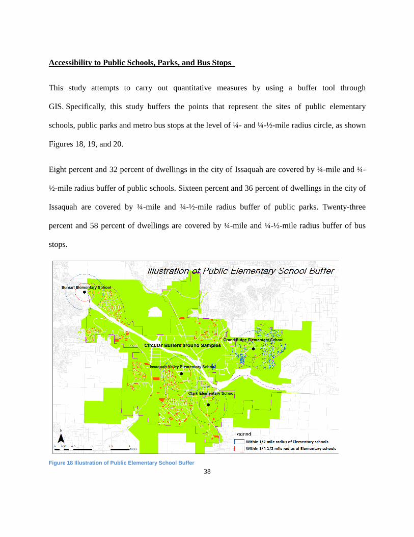
Accessibility to Public Schools, Parks, and Bus Stops

This study attempts to carry out quantitative measures by using a buffer tool through

GIS. Specifically, this study buffers the points that represent the sites of public elementary

schools, public parks and metro bus stops at the level of ¼ - and ¼ -½ -mile radius circle, as shown

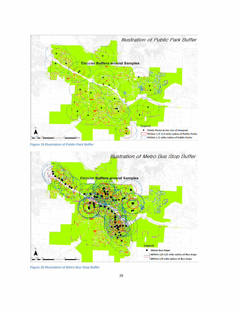
Figures 18, 19, and 20.

Eight percent and 32 percent of dwellings in the city of Issaquah are covered by ¼ -mile and ¼ -

½ -mile radius buffer of public schools. Sixteen percent and 36 percent of dwellings in the city of

Issaquah are covered by ¼ -mile and ¼ -½ -mile radius buffer of public parks. Twenty-three

percent and 58 percent of dwellings are covered by ¼ -mile and ¼ -½ -mile radius buffer of bus

stops.

Figure 18 Illustration of Public Elementary School Buffer

39

Figure 19 Illustration of Public Park Buffer

Figure 20 Illustration of Metro Bus Stop Buffer

40

4.4 Summary of Variables

For the hedonic pricing model to precisely estimate the different components of single family

housing, the priority for consideration about purchasing housing must be the housing attributes.

As such, this study attempts to reflect all of the housing attributes provided by WAGDA and Tax

Assessments. Also, this study reflects a wide array of variables for location, neighborhood,

market, and socio-demographic characteristics.

Dependent Variables

This study has two dependent variables: (1) the Sales Price (Linear form) for single family

housing values, and (2) the Log Sales Price (Semi log form) for single family housing values.

Independent Variables

Site Characteristics

Site attributes include two variables. (1) Log Lot is the log transformation of lot size, indicating

that each additional square foot of land does not increase land value as significantly as the prior

square foot of land. For several communities, the additional value of a square foot of lot

diminishes with size (Eppli and Tu 1999). (2) Parking is the number of the attached and

detached garages.

Interior Characteristics

There are many attributes to measure the interior characteristics. (1) Living Area is one of main

attributes, indicating the square footage of the interior living area, excluding the finished

basement. (2) Basement is used to figure whether a home has a basement (a value of 1 if

41

housing has a basement and 0 otherwise, so it is a binary variable). (3) Bedroom is the number

of rooms in the home. (4) Bathroom corresponds to the number of bathrooms in the home, with

half bathrooms counted as one half and three fourths bathrooms counted as three fourths. (5)

Fireplace is the number of fireplaces in the home.

Exterior Characteristics

There are many attributes to measure the exterior characteristics. Exterior characteristics

generally are described by binary variables representing porch, deck, and number of stories. (1)

Open porch is whether a home has an open porch (a value of 1 if housing has an open porch and

0 otherwise). (2) Deck is whether a home has a deck (a value of 1 if housing has a deck and 0

otherwise). Similarly, both (3) Story 1 (a value of 1 if housing has 1 story and 0 otherwise) and

(4) Story 3 (a value of 1 if housing has 3 stories and 0 otherwise) are binary variables, with

Story 2 as a reference variable. The most common exterior characteristic is the reference

variable.

Quality Characteristics

One of major variables for quality is age. The (1) Age variable is the age of housing in years. The

(2) Age square variable is one that squares the Age variable. The Age square variable allow for

the value of housing not only to reduce with age, but also to avoid reducing housing values based

on a nonlinear relationship between housing value and age. That is, the age of housing may not

be linearly correlated with price. Several studies indicates a U-shape relation between housing

value and age (Coulson and McMillen 2008; Coulson and Lahr 2005). The (3) New variable is

included to isolate the effect of new housing, including the first sales transaction after

42

construction. Last, another proxy for quality is (4) Grade. The Grade variable indicates

residential building grade in terms of construction quality. It has a range of 1 (Lowest) to 13

(Highest) along with 8 (Average). This grade increases the accuracy of analysis by narrowing the

range of observations.

Location Characteristics

Location is also critical in estimating the housing values. For instance, consumers’ housing

preference may vary according to location characteristics such as tax rates, air pollution, and

crime. As shown in Figure 17, the City of Issaquah is included in a boundary consisting of eight

census tracts. (1) Issaquah Highlands (Tract 322.10), which represents the study area, is used

to recognize locational differences (a value of 1 if housing is located in Issaquah Highlands and 0

otherwise).9 The coefficient of this variable is the most important number in this study.

Neighborhood Characteristics

This study intends to measure and quantify built environments. This study attempts to reflect the

effect of each school district through (1) Test Scores of four public elementary schools. Figures

18, 19, and 20 present examples about how to measure ¼ - and ¼ -½ mile radius areas through

utilizing a GIS buffer tool. Based on this method, (2) Within ¼ -mile radius of Elementary

School and (3) Within ¼ -½ -mile radius of Elementary School represent dwellings within ¼ -

mile radius and ¼ -½ -mile radius of elementary schools that are included in this study. (4) Within

¼ -mile radius of Bus stops and (5) Within ¼ -½ -mile radius of Bus stops that represents

dwellings within ¼ -mile radius and ¼ -½ -mile radius of Bus stops are included in this study. (6)

9 Among the eight census tracts, only 322.10 covers the area of Issaquah Highlands., while the others (322.08,

234.04, 250.03, 250.06, 321.04, 321.03, and 321.02) cover the surrounding areas in the city of Issaquah.

43

Within ¼ -mile radius of Public parks and (7) Within ¼ -½ -mile radius of Public parks that

represent dwellings within ¼ -mile radius and ¼ -½ -mile radius of public parks are included in

this study.

Market Characteristics

(1) Year 12 and (2) Year 14 that represent the time of sale transaction over the three-year period

January 2012 through December 2014 are included in this study. These variables are expected to

show the housing market dynamics in the study area from 2012 to 2014, along with Year 13 as a

reference variable. (3) Olympics View, (4) Cascades View, (5) Territorial View, (6) Seattle

Sky View, and (7) Lake Sammamish View variables are used to reflect other significant

amenities on neighborhood characteristics (a value of 1 if housing has a view and 0 otherwise).

Also, (8) Traffic Noise (Moderate 1, High 2, Extreme 3) is included in this study.

Socio-Demographic Characteristics

(1) Median Income of Household that indicates the wealth of neighborhood is included based

on census tract level data. Also, (2) Median Age of Household and (3) Ratio of White

Residents are used to reflect other significant factors of socio-demographic characteristics.

44

Table 5 Variable descriptions

Attribute Description

Dependent Variables

Sale Price Sale price recorded on the deed

Log Sale Price Natural logarithm of sale price

Site Characteristics

Lot Square footage of lot

Log Lot Natural logarithm of lot size

Parking Number of attached and detached parking spaces

Interior Characteristics

Living Area Square footage of living area, excluding finished basement

Basement Binary variable 1 if the house has a basement, otherwise 0

Bedroom Number of bedrooms

Bathroom Number of bathrooms

Fireplace Number of fireplaces

Exterior Characteristics

Open Porch Binary variable 1 if the house has an open porch, otherwise 0

Deck Binary variable 1 if the house has a deck, otherwise 0

Story 1 Binary variable 1 if the number of stories is 1, otherwise 0

Story 2 Reference variable (Including stories 1.5)

Story 3 Binary variable 1 if the number of stories is 3, otherwise 0 (Including stories 2.5)

Quality Characteristics

Age Housing age in years

Age Squared Age squared

Newa Binary variable 1 if the the housing is new, otherwise 0

Grade 6 Binary variable 1 if the the construcion quality is grade 6, otherwise 0

Grade 7 Binary variable 1 if the the construcion quality is grade 7, otherwise 0

Grade 8b Reference variable

Grade 9 Binary variable 1 if the the construcion quality is grade 9, otherwise 0

Grade 10 Binary variable 1 if the the construcion quality is grade 10, otherwise 0

Grade 11 Binary variable 1 if the the construcion quality is grade 11, otherwise 0

Location Characteristics

Issaquah Highlands (Tracts 322.10)c Binary variable 1 if the the housing is located in Issaquah Highlands (Tract 322.10), otherwise 0

Neighborhood Characteristics

Test Scores Test Score for the four public elementary schools

Within ¼ - mile radius of Public Elementary Schools Binary variable 1 if the the housing is located within ¼ - mile radius of Public Elementary Schools, otherwise 0

Within ¼ -½ - mile radius of Public Elementary Schools Binary variable 1 if the the housing is located within ¼ -½ - mile radius of Public Elementary Schools, otherwise 0

Within ¼ - mile radius of Bus stops Binary variable 1 if the the housing is located within ¼ - mile radius of Bus stops, otherwise 0

Within ¼ -½ - mile radius of Bus stops Binary variable 1 if the the housing is located within ¼ -½ - mile radius of Bus stops, otherwise 0

Within ¼ - mile radius of Public parks Binary variable 1 if the the housing is located within ¼ - mile radius of Public parks, otherwise 0

Within ¼ -½ - mile radius of Public parks Binary variable 1 if the the housing is located within ¼ -½ - mile radius of Public parks, otherwise 0

Market Characteristics

Year 12 Binary variable 1 if the transaction occurred in 2012, otherwise 0

Year 13 Reference variable

Year 14 Binary variable 1 if the transaction occurred in 2014, otherwise 0

Olympics View Binary variable 1 if the the housing has a Olympics view, otherwise 0

Cascades View Binary variable 1 if the the housing has a Cascades view, otherwise 0

Territorial View Binary variable 1 if the the housing has a Territorial view, otherwise 0

Seattle Sky View Binary variable 1 if the the housing has a Seattle Sky view, otherwise 0

Lake Sammamish View Binary variable 1 if the the housing has a Lake Sammamsh view, otherwise 0

Traffic Noise Traffic noise (Moderate 1, High 2, Extreme 3)

Socio-demographic Characteristics

Median Income of Household Household annual median income based on Census tract level

Ratio of White Residents Ratio of white residents based on Census tract level

Median Age of Household Median household age based on Census tract level

a If a built year and a sale year are same, it is included in New.

c The City of Issaquah is covered by a group of 8 census tracts. Among 8 tracts, only tract 322.10 includes Issaquah Highlands.

b The quality of construction is defined by the King County Department of Assessment on a scale from 1 to 13. The reference variables is Grade 8 (Average).

45

Chapter 5 Methodology

5.1 Research Design

This study examines the impact of New Urbanism on single family housing values in the city of

Issaquah. To reduce bias and increase accuracy in research, various methods are adopted to

assess the impact of neighborhood externalities on single family housing values. Among them, a

straightforward mean of determining the price differential between a New Urbanism community

and a conventional community is to compare 2012-2014 average sale prices for recent

transactions.

As shown in Table 7, the average sale price in Issaquah Highlands ($638,358) was higher than

outside of Issaquah Highlands ($608,673) from 2012 to 2014. That is, a consumer was willing to

pay approximately $30,000 more to reside in a New Urbanism community rather than a

conventional community.

Even though comparing averages can be instructive, it can also include many shortages because

this mean is considered under the assumption that all housing attributes between two

communities are the same. However, several differences between the two communities exist, and

it may include housing, location, neighborhood, market, and socio-demographic characteristics.

If such differences in characteristics cannot be controlled, comparing averages will not be

persuasive as a research mean.

Thus, a more sophisticated statistical tool is required to assess the differences, one of which is

multiple regression analysis. Regression analysis provides a quantitative tool to test the behavior

46

of consumers when purchasing single family housing. Also, the application of regression to

housing valuation is referred to as the hedonic pricing model. Particularly, the focus of this study

is the coefficient of one independent variable (Issaquah Highlands (Tract 322.10)) that is a proxy

for a community developed according to the principles of New Urbanism. It indicates how much

of a premium people are willing to pay for houses in a New Urbanism community. The results of

the hedonic pricing model will allow planners, developers, and researchers to draw conclusions

through statistical relationships.

47

5.2 Research Method

Hedonic Pricing Model

This study uses the hedonic pricing technique to assess the impact of New Urbanism on the value

of single family residences. Hedonic pricing analysis is a multiple regression model that

deconstructs housing values into measurable prices and quantities, which helps estimate the

extent to which each factor affects the price for different dwelling units in different places

(Malpezzi 2003; Yan, Delmelle, and Duncan 2012).

The hedonic pricing model enables more than two independent variables to simultaneously affect

single family housing values, indicating that extra independent variables can be added to the

regression model to better explain the relative importance of each attribute on housing values

(Eppli and Tu 1999).

In this study, to estimate the impact of New Urbanism on single family housing values, the

hedonic price model uses (1) Site Characteristics, (2) Interior Characteristics, (3) Exterior

Characteristics, (4) Quality Characteristics, (5) Location Characteristics, (6) Neighborhood

Characteristics, (7) Market Characteristics, and (8) Socio-demographic Characteristics to predict

the sale price of housing units.

Keeping other variables constant, the change in the sale price resulting from a change in any

particular attribute is called the hedonic price, or implicit price, of an attribute (Yan, Delmelle,

and Duncan 2012).

There is an assumption that a housing sale price P(H) is a function of S1, which indicates Site

48

Characteristics; I, Interior Characteristics; E, Exterior Characteristics; Q, Quality Characteristics;

L, Location Characteristics; N, Neighborhood Characteristics; M, Market Characteristics; and S2,

Socio-demographic Characteristics (Hess and Almeida 2007; Yan, Delmelle, and Duncan 2012).

The conceptual hedonic pricing model is:

P(H) = f (S1, I, E, Q, L, N, M, S2),

Several variables are transformed:

Sale price or ln(Sale price) = β0 + βixi + e,

where β0 is the constant, βi (i=37) are coefficients, and xi (i=37) are the variables shown in Table

10 and Table 11.

By employing the hedonic pricing model, this study examines the null hypothesis that the sale

prices of houses in Issaquah Highlands will not be significantly different than those in

surrounding areas. In other words, the null hypothesis is that the coefficient of the binary variable

is zero, indicating that consumers are willing to pay similar prices for houses in Issaquah

Highlands and for houses in the surrounding conventional subdivisions.

49

Functional Form

Choosing the proper functional form of the hedonic pricing model plays a pivotal role in

reducing inconsistent coefficients. Based on the literature review, early studies using the hedonic

pricing model chose the basic functional form, such as linear, semi-log, and log-log, for their

simplicity.

Unfortunately, theory offers no guidelines for the functional form specification (Eppli and Tu

1999). So, Rosen (1974) suggests using a goodness-of-fit criterion in choosing the functional

form. Also, most researchers use the goodness-of-fit criterion in comparing the basic and the

more complicated forms derived from the Box-Cox transformation.10

Early studies favor the

Box-Cox forms, as the transformation often creates the best fit for the data.

However, other studies present three shortcomings of the Box-Cox transformation. Following the

study by Linneman (1980), it is not suitable to use independent variables that are dichotomous.

Also, the large estimated coefficients reduce the accuracy of any single coefficient. In addition,

based on errors produced in estimating the hedonic prices or implicit prices, Cropper, Deck, and

McConnell (1988) realize that Box-Cox forms outperform the basic restricted forms when all

attributes are observed.

Using only a single functional form might be insufficient to draw a compelling conclusion.

However, this study focuses on how much of a premium consumers are willing to pay for New

Urbanism. The study by Cropper, Deck, and McConnell (1988) suggests that the functional form

10

Box and Cox (1964) developed a model that determines the functional specification that provides the best fit in

terms of log likelihood. For more information, see Box and Cox (1964).

50

providing the best goodness-of-fit does not necessarily generate the most accurate estimate of

implicit price.

Consequently, this study has estimated a series of models with transformations of the dependent

variable only. Thus, the results of semi-log form and linear form respectively are presented in

this study.

Most previous studies mention linear form and semi-log form. Semi-log is a common form of a

standard hedonic pricing model to examine the effects of built environment on property values

(Song and Knaap 2003; 2004). To ensure that the identified price differential is not caused by

using only semi-log functional form, additional estimation is conducted by using the linear form

(Tu and Eppli 2001; Randall 2002). The linear form allows an interpretation of the coefficients in

dollars. Also, using the natural logarithm of the sale price (semi-log) allows an estimation of a

potential percentage change in sale price.

This study assumes that sale property values reflect consumers’ preferences for New Urbanism

neighborhoods, which would be associated with consumers’ willingness to pay.

51

Chapter 6 Results

6.1 T-Test Independent Samples

T-test allows comparison of Issaquah Highlands and outside of Issaquah Highlands in terms of

different average single family housing values. The independent-Samples T-test (or Independent

T-test, for short) compares the means between two unrelated groups on the same continuous,

dependent variable.

Null Hypotheses

The hypothesis is that the two groups in the City of Issaquah have different single family housing

values, so the null hypothesis is that they do not have different single family housing values.

Table 6 Independent T-test result

Result

First, F-test is performed. If the P-value (0.265) is greater than 0.05, the variances of the two

samples can be assumed to be equal. The numbers (yellow cells) in “Equal variances assumed”

should be considered. Then, the group means are significantly different because the P-value of

0.045 in the “Sig. (2-tailed)” row is less than 0.05. As a result, the null hypothesis is rejected, and

the conclusion is that the two means do indeed differ significantly.

Lower Upper

Equal variances

assumed1.244 .265 -2.003 1073 .045 -29684.912 14821.495 -58767.314 -602.510

Equal variances

not assumed-2.037 1072.449 .042 -29684.912 14574.729 -58283.132 -1086.692

Std.Error

Difference

95% Confidence Interval of

the Mean

Sale Price

Levene's Test for

Equality of VariancesT-test for Equality of Means

F Sig. t df Sig.(2-tailed)Mean

Difference

52

6.2 Descriptive Statistics

Table 7 presents summary statistics for dependent and independent variables used in the hedonic

pricing models. On average, more expensive properties are located in Issaquah Highlands

($638,358), followed by All Sales ($622,066), and Out of Issaquah Highlands ($608,673). 45.1

percent of sampled properties are in Issaquah highlands, and 54.9 percent are outside of Issaquah

Highlands, based on the final data set of 1,075 dwellings.

In terms of site and housing characteristics, dwellings in Issaquah Highlands have much smaller

lots (4,664 sq. ft.) than dwellings in surrounding areas (10,444 sq. ft.). In addition, homes in

Issaquah Highlands have younger structure ages (6.83) than the other areas (25.16). Except for

the above two points, there are not obvious significant differences between them.

Interestingly, there is a 67-year-old house in Issaquah Highlands, even though the first residents

arrived in 1998 and construction began in 1996. Clearly, there were some existing houses on the

site.

For neighborhood characteristics, homes in Issaquah Highlands have a higher test score (0.83)

than others (0.76). This might be a significant effect in determining housing values.

In terms of market characteristics, there have been similar numbers of sale transactions over the

three-year period from 2012 to 2014 in the City of Issaquah. Dwellings in Issaquah Highlands

contain more and varying views relative to surrounding areas.

For socio-demographic characteristics, the median household income in Issaquah Highlands

($121,061) is higher than the others ($107,136). The median age of household in Issaquah

53

Highlands (35.0) is relatively lower than that in surrounding areas (39.2). These categorized

numbers in Issaquah Highlands are absolutely identical, because census tract level data which

covers Issaquah Highlands has been applied.

54

Table 7 Descriptive statistics for single family housing

Min Max Mean Std. Div. Min Max Mean Std. Div. Min Max Mean Std. Div.

Dependent Variables

Sale Price 150000.00 2600000.00 622066.68 242154.57 225000.00 1700000.00 638358.87 218250.53 150000.00 2600000.00 608673.96 259583.81

Log Sale Price 11.92 14.77 13.28 0.33 12.32 14.35 13.32 0.30 11.92 14.77 13.25 0.35

Site characteristics

Lot 1428.00 85499.00 7836.82 8012.99 1428.00 44866.00 4664.95 3273.45 1850.00 85499.00 10444.20 9652.94

Parking 0.00 2.00 0.97 0.40 0.00 2.00 0.92 0.30 0.00 2.00 1.02 0.46

Interior characteristics

Living Area 820.00 5030.00 2326.91 735.65 1050.00 5030.00 2422.81 674.96 820.00 4340.00 2248.08 773.72

Basement 0.00 1.00 0.44 0.50 0.00 1.00 0.29 0.45 0.00 1.00 0.57 0.50

Bedroom 0.00 7.00 3.61 0.74 0.00 7.00 3.54 0.72 0.00 6.00 3.67 0.76

Bathroom 0.00 5.50 2.67 0.67 0.00 5.50 2.79 0.59 0.00 4.75 2.57 0.71

Fireplace 0.00 5.00 1.34 0.71 0.00 4.00 1.12 0.63 0.00 5.00 1.53 0.71

Exterior characteristics

Open Porch 0.00 1.00 0.76 0.43 0.00 1.00 0.87 0.34 0.00 1.00 0.66 0.47

Deck 0.00 1.00 0.42 0.49 0.00 1.00 0.23 0.42 0.00 1.00 0.57 0.50

Story 1 0.00 1.00 0.19 0.39 0.00 1.00 0.02 0.14 0.00 1.00 0.33 0.47

Story 3 0.00 1.00 0.03 0.16 0.00 1.00 0.05 0.23 0.00 1.00 0.00 0.06

Quality characteristics

Age 0.00 89.00 16.89 16.31 0.00 67.00 6.83 4.90 0.00 89.00 25.16 17.71

New 0.00 1.00 0.20 0.40 0.00 1.00 0.29 0.46 0.00 1.00 0.12 0.32

Grade 6 0.00 1.00 0.01 0.11 0.00 0.00 0.00 0.00 0.00 1.00 0.02 0.15

Grade 7 0.00 1.00 0.11 0.31 0.00 1.00 0.07 0.25 0.00 1.00 0.14 0.35

Grade 9 0.00 1.00 0.27 0.44 0.00 1.00 0.32 0.47 0.00 1.00 0.23 0.42

Grade 10 0.00 1.00 0.13 0.33 0.00 1.00 0.09 0.29 0.00 1.00 0.15 0.36

Grade 11 0.00 1.00 0.07 0.25 0.00 1.00 0.07 0.26 0.00 1.00 0.06 0.24

Location characteristics

Isssaquah Highlands (Tracts 322.10) 0.00 1.00 0.45 0.50 1.00 1.00 1.00 0.00 0.00 0.00 0.00 0.00

Neighborhood characteristics

Test Scores 0.74 0.84 0.79 0.04 0.76 0.84 0.83 0.02 0.74 0.80 0.76 0.03

Within ¼ - mile radius of Public Elementary schools 0.00 1.00 0.08 0.27 0.00 1.00 0.05 0.21 0.00 1.00 0.10 0.30

Within ¼ -½ - mile radius of Public Elementary schools 0.00 1.00 0.32 0.47 0.00 1.00 0.46 0.50 0.00 1.00 0.21 0.41

Within ¼ - mile radius of Bus stops 0.00 1.00 0.16 0.36 0.00 1.00 0.04 0.19 0.00 1.00 0.25 0.43

Within ¼ -½ - mile radius of Bus stops 0.00 1.00 0.36 0.48 0.00 1.00 0.31 0.46 0.00 1.00 0.40 0.49

Within ¼ - mile radius of Public parks 0.00 1.00 0.23 0.42 0.00 1.00 0.07 0.26 0.00 1.00 0.35 0.48

Within ¼ -½ - mile radius of Public parks 0.00 1.00 0.58 0.49 0.00 1.00 0.63 0.48 0.00 1.00 0.54 0.50

Market characteristics

Year 12 0.00 1.00 0.32 0.47 0.00 1.00 0.34 0.47 0.00 1.00 0.31 0.46

Year 14 0.00 1.00 0.31 0.46 0.00 1.00 0.28 0.45 0.00 1.00 0.33 0.47

Olympics View 0.00 1.00 0.04 0.20 0.00 1.00 0.10 0.30 0.00 0.00 0.00 0.00

Cascades View 0.00 1.00 0.03 0.16 0.00 0.00 0.00 0.00 0.00 1.00 0.05 0.22

Territorial View 0.00 1.00 0.20 0.40 0.00 1.00 0.21 0.41 0.00 1.00 0.18 0.39

Seattle Sky View 0.00 1.00 0.01 0.12 0.00 1.00 0.03 0.18 0.00 0.00 0.00 0.00

Lake Sammamish View 0.00 1.00 0.05 0.23 0.00 1.00 0.06 0.23 0.00 1.00 0.05 0.22

Traffic Noise 0.00 3.00 0.08 0.37 0.00 2.00 0.04 0.21 0.00 3.00 0.11 0.45

Socio-demograohic characteristics

Median Income of Household 56858.00 134180.00 113418.65 24040.67 121061.00 121061.00 121061.00 0.00 56858.00 134180.00 107136.37 31084.25

Ratio of White Residents 0.68 0.97 0.74 0.06 0.71 0.71 0.71 0.00 0.68 0.97 0.77 0.07

Median Age of Household 35.00 49.00 37.31 2.91 35.00 35.00 35.00 0.00 37.00 49.00 39.20 2.73

AttributeAll Sales (n=1075) Issaquah Highlands (n=485) Out of Issaquah Highlands (n=590)

55

6.3 Hedonic Pricing Model and Results

This section presents the results of the hedonic pricing model for the impact of New Urbanism

on single family housing values in the City of Issaquah. The null hypothesis in this analysis is

that consumers pay the same prices for houses in a New Urbanism community and in a

conventional subdivision.

To study whether consumers pay a premium or discount to reside in Issaquah Highlands, the

coefficient in Location characteristics (Issaquah Highlands (Tract 322.10)) is the most valuable

number in this research. This Issaquah Highlands (Tract 322.10) variable measures the housing

price differential between a New Urbanism community and a conventional subdivision along

with controlling for other independent variables for the price variation.

Multi-Collinearity Test

Table 9 contains all the characteristics included in the model. The strength of this specification

encourages the model to minimize the possibility of inconsistent estimates caused by omitted

variables and to maximize the explanatory power of estimates (Eppli and Tu 1999). In contrast,

this fully specified model may generate a collinearity issue if there are highly correlated

variables.

This study uses variance inflation factor (VIF) values as a test for multi-collinearity.11

VIF

values below 10 indicate that multi-collinearity is not an issue in the model (Bae et al. 2007;

11

Multi-collinearity is a phenomenon where two or more variables in a multiple regression model are highly

correlated with each other. It indicates that one variable can be linearly predicted from the others with some degree

of accuracy.

56

Sohn, Moudon, and Lee 2012). If the test detects severe multi-collinearity, some variables should

be deleted to reduce an issue. Severe multi-collinearity is detected in the “Age,” “Age Squared,”

and “Issaquah Highlands (Tract 322.10)” variables.

This study estimates a linear regression model. The correlation between “Age” and “Age

Squared” is 0, since there is no linear relationship. That is, the perfect collinearity is due to a

“perfect” linear relationship. However, in this case, the variables age and age square are not

linearly correlated.

For the “Issaquah Highlands (Tract 322.10)” variable, there is a correlation between an “Issaquah

Highlands (Tract 322.10)” and a “Test Scores” variable, which indicates a value greater than

0.800 through a Pearson Correlation Coefficient test (see Table 8). Correlation coefficients

whose magnitude is greater than 0.8 indicates a strong correlation between the two variables,

which leads to multi-collinearity (Zou, Tuncali, and Silverman 2003).

Even though a “Test Scores” variable for school districts has a very significant impact on

housing value (see Table 9), this study removed a “Test Scores” variable to avoid multi-

collinearity.

57

Table 8 Pearson Correlation Matrix

Sale Price Log Lot Parking Living Basement Bedrooms Bathroom FireplaceOpen

PorchDeck Story1 Story3 Age

Age

SquaredNew Grade 6 Grade 7 Grade 9 Grade 10 Grade 11

Pearson

Correlation 1Sig. (2-tailed)

Pearson

Correlation .182** 1

Sig. (2-tailed) .000Pearson

Correlation .145** -.043 1

Sig. (2-tailed) .000 .154Pearson

Correlation .713**

.169**

.094** 1

Sig. (2-tailed) .000 .000 .002Pearson

Correlation .119** .037 .246** -.195** 1Sig. (2-tailed) .000 .229 .000 .000

Pearson

Correlation .375** .193** .111** .435** .187** 1Sig. (2-tailed) .000 .000 .000 .000 .000

Pearson

Correlation .581** -.102** .149** .553** .315** .526** 1Sig. (2-tailed) .000 .001 .000 .000 .000 .000

Pearson

Correlation .416** .399** .088** .356** .178** .291** .266** 1Sig. (2-tailed) .000 .000 .004 .000 .000 .000 .000

Pearson

Correlation .231** -.257** -.022 .344** -.012 .103** .357** -.063* 1Sig. (2-tailed) .000 .000 .476 .000 .702 .001 .000 .040

Pearson

Correlation .135** .341** .104** -.033 .439** .203** .119** .265** -.044 1Sig. (2-tailed) .000 .000 .001 .286 .000 .000 .000 .000 .150

Pearson

Correlation -.279** .432** -.014 -.519** .281** -.146** -.452** .102** -.435** .287** 1Sig. (2-tailed) .000 .000 .639 .000 .000 .000 .000 .001 .000 .000

Pearson

Correlation .069* -.096** -.004 .121** -.016 .023 .103** .078* .093** .004 -.080** 1Sig. (2-tailed) .023 .002 .907 .000 .597 .453 .001 .011 .002 .906 .009

Pearson

Correlation -.261** .618** -.177** -.363** .023 -.067* -.501** .185** -.453** .217** .688** -.075* 1Sig. (2-tailed) .000 .000 .000 .000 .443 .029 .000 .000 .000 .000 .000 .014

Pearson

Correlation -.252** .509** -.225** -.379** .058 -.095** -.466** .096** -.412** .185** .649** -.036 .946** 1Sig. (2-tailed) .000 .000 .000 .000 .059 .002 .000 .002 .000 .000 .000 .232 0.000

Pearson

Correlation .041 -.348** .132** -.070* .237** .027 .241** -.192** .101** .064* -.223** .022 -.471** -.291** 1Sig. (2-tailed) .182 .000 .000 .022 .000 .373 .000 .000 .001 .037 .000 .477 .000 .000

Pearson

Correlation -.143** .070* -.237** -.191** -.003 -.139** -.217** -.161** -.126** -.014 .236** -.019 .333** .446** -.057 1Sig. (2-tailed) .000 .021 .000 .000 .920 .000 .000 .000 .000 .644 .000 .538 .000 .000 .062

Pearson

Correlation -.313** .118** -.073* -.391** .002 -.098** -.343** -.157** -.213** -.023 .361** -.057 .392** .389** -.166** -.040 1Sig. (2-tailed) .000 .000 .017 .000 .953 .001 .000 .000 .000 .443 .000 .061 .000 .000 .000 .188

Pearson

Correlation .095** .034 .082** .316** -.157** .068* .075* .007 .183** -.069* -.195** -.034 -.181** -.218** -.180** -.070* -.212** 1Sig. (2-tailed) .002 .271 .007 .000 .000 .026 .013 .811 .000 .025 .000 .271 .000 .000 .000 .022 .000

Pearson

Correlation .262** -.055 .144** .267** .149** .101** .241** .142** .143** .043 -.163** .132** -.213** -.169** .165** -.044 -.132** -.230** 1Sig. (2-tailed) .000 .070 .000 .000 .000 .001 .000 .000 .000 .156 .000 .000 .000 .000 .000 .154 .000 .000

Pearson

Correlation .567** .192** .036 .458** .095** .205** .349** .317** .089** .086** -.101** .004 -.108** -.111** -.019 -.031 -.093** -.162** -.101** 1Sig. (2-tailed) .000 .000 .233 .000 .002 .000 .000 .000 .003 .005 .001 .908 .000 .000 .537 .317 .002 .000 .001

Pearson

Correlation .061* -.525** -.116** .118** -.280** -.091** .162** -.293** .239** -.343** -.399** .157** -.559** -.467** .222** -.104** -.119** .098** -.095** .030Sig. (2-tailed) .045 .000 .000 .000 .000 .003 .000 .000 .000 .000 .000 .000 .000 .000 .000 .001 .000 .001 .002 .328

Pearson

Correlation .169** -.323** -.081** .215** -.416** -.078* .076* -.177** .136** -.291** -.329** .065* -.393** -.360** .043 -.091** -.110** .152** -.094** .108**

Sig. (2-tailed) .000 .000 .008 .000 .000 .010 .013 .000 .000 .000 .000 .033 .000 .000 .156 .003 .000 .000 .002 .000Pearson

Correlation .065* .042 -.006 .054 .090** -.001 .101** .050 .036 .098** -.045 -.048 -.027 -.032 .039 -.033 -.035 .120** .005 -.008Sig. (2-tailed) .033 .170 .836 .076 .003 .968 .001 .101 .245 .001 .141 .119 .381 .298 .206 .273 .252 .000 .877 .802

Pearson

Correlation -.182** -.152** -.087** -.191** -.224** -.172** -.145** -.222** -.060* -.071* -.007 -.063* -.028 -.009 .069* .061* .053 -.087** -.153** -.119**

Sig. (2-tailed) .000 .000 .004 .000 .000 .000 .000 .000 .048 .020 .829 .040 .357 .776 .024 .044 .080 .004 .000 .000Pearson

Correlation -.121** .250** -.131** -.177** -.051 -.079** -.236** .032 -.212** .085** .241** -.070* .390** .394** -.148** .245** .122** -.110** -.101** -.042Sig. (2-tailed) .000 .000 .000 .000 .097 .009 .000 .301 .000 .006 .000 .021 .000 .000 .000 .000 .000 .000 .001 .172

Pearson

Correlation -.005 -.079** .142** -.072* .177** .124** .105** .012 -.024 .149** -.010 -.001 -.090** -.071* .316** -.086** -.100** -.066* -.161** -.098**

Sig. (2-tailed) .862 .009 .000 .018 .000 .000 .001 .685 .434 .000 .751 .983 .003 .020 .000 .005 .001 .030 .000 .001Pearson

Correlation -.038 .167** .003 .010 -.041 .028 -.141

**.100

**-.065

* .048 .119**

-.089**

.233**

.181**

-.175**

.075* .052 .035 -.106

** -.028Sig. (2-tailed) .208 .000 .912 .749 .176 .353 .000 .001 .034 .116 .000 .004 .000 .000 .000 .015 .087 .258 .001 .352

Pearson

Correlation .069* -.076* .084** -.005 .013 .010 .027 -.004 -.011 .037 -.050 .031 -.084** -.046 .124** -.020 -.026 -.138** .155** .095**

Sig. (2-tailed) .023 .012 .006 .875 .662 .753 .376 .891 .716 .224 .104 .305 .006 .130 .000 .520 .388 .000 .000 .002Pearson

Correlation -.226**

-.116** .016 -.052 .012 -.008 -.004 -.074

* .030 .017 -.045 .026 -.031 -.020 .106** -.008 -.028 .005 -.043 -.038

Sig. (2-tailed) .000 .000 .595 .086 .693 .797 .905 .016 .321 .567 .139 .403 .310 .523 .000 .782 .352 .860 .156 .214Pearson

Correlation .240** .108** -.011 .079** .017 .030 .019 .110** -.030 .020 .037 .044 .072* .033 -.242** -.005 .034 .007 .048 .060Sig. (2-tailed) .000 .000 .724 .009 .588 .333 .534 .000 .326 .502 .229 .151 .018 .276 .000 .874 .260 .821 .119 .050

Pearson

Correlation .364** .038 .026 .274

**.075

*.186

**.266

**.173

**.089

**.133

**-.081

** -.006 -.130**

-.112** -.015 -.025 -.075

* -.038 .070*

.346**

Sig. (2-tailed) .000 .218 .401 .000 .013 .000 .000 .000 .003 .000 .008 .834 .000 .000 .635 .421 .014 .217 .022 .000Pearson

Correlation .166** .159** .082** .188** .088** .089** .147** .126** .030 .074* -.025 .008 -.027 -.055 -.084** -.019 -.059 .050 .089** .137**

Sig. (2-tailed) .000 .000 .008 .000 .004 .003 .000 .000 .324 .015 .411 .800 .384 .071 .006 .524 .052 .103 .003 .000Pearson

Correlation .435** .026 .109

**.254

**.348

**.241

**.450

**.155

**.187

**.218

**-.139

** -.037 -.238**

-.194**

.185** -.057 -.143

** .006 .145**

.246**

Sig. (2-tailed) .000 .392 .000 .000 .000 .000 .000 .000 .000 .000 .000 .229 .000 .000 .000 .063 .000 .852 .000 .000Pearson

Correlation .354** .079** .027 .213** .092** .137** .231** .136** .070* .067* -.021 .028 -.092** -.068* .094** -.014 -.043 -.075* .023 .338**

Sig. (2-tailed) .000 .009 .371 .000 .003 .000 .000 .000 .022 .027 .496 .357 .002 .026 .002 .644 .159 .014 .452 .000Pearson

Correlation .403**

.105** -.004 .163

**.205

**.149

**.255

**.138

** .032 .119** -.024 .012 -.030 -.014 .106

** -.028 -.071*

-.073* .007 .281

**

Sig. (2-tailed) .000 .001 .892 .000 .000 .000 .000 .000 .300 .000 .433 .697 .319 .637 .000 .365 .020 .017 .812 .000Pearson

Correlation .103** .072* .008 .032 .112** .078* .084** -.039 .008 .087** .025 -.035 -.005 .042 .150** .178** -.034 .065* -.066* .076*

Sig. (2-tailed) .001 .019 .793 .294 .000 .010 .006 .200 .786 .004 .408 .252 .879 .173 .000 .000 .267 .033 .031 .012Pearson

Correlation .251**

-.424**

.223**

.226** -.034 .026 .217

**-.061

*.216

**-.200

**-.391

** .046 -.496**

-.472**

.188**

-.201**

-.234**

.067*

.153**

.129**

Sig. (2-tailed) .000 .000 .000 .000 .269 .395 .000 .047 .000 .000 .000 .134 .000 .000 .000 .000 .000 .028 .000 .000Pearson

Correlation -.196** .552** -.103** -.288** -.006 .008 -.351** .180** -.402** .239** .514** -.066* .736** .647** -.287** .151** .233** -.167** -.229** -.131**

Sig. (2-tailed) .000 .000 .001 .000 .835 .784 .000 .000 .000 .000 .000 .031 .000 .000 .000 .000 .000 .000 .000 .000Pearson

Correlation -.107**

.562**

-.072*

-.112**

.123**

.075*

-.144**

.213**

-.238**

.288**

.394**

-.116**

.552**

.487**

-.221**

.154**

.126**

-.082** -.006 -.070

*

Sig. (2-tailed) .000 .000 .018 .000 .000 .014 .000 .000 .000 .000 .000 .000 .000 .000 .000 .000 .000 .007 .842 .021*. Significant at p<0.05, **. Significant at P<0.01Yellow cells: Pearson correlation value > 0.8

Lake

Sammamish

TrafficNoi

Income

White

Age

SeattleSky

School 0.25

School

0.25-0.5

Bus stop

0.25

Bus stop

0.25-0.5

Park 0.25

Park

0.25-0.5

Year 12

Year 14

Olympics

Cascades

Territorial

Test Scores

Story1

Story3

Age

Age

Squared

New

Grade 6

Grade 7

Grade 9

Grade 10

Grade 11

Issaquah

Highlands

Deck

Sale Price

Log Lot

Parking

Living

Basement

Bedrooms

Bathroom

Fireplace

Open

Porch

58

Table 8 Continued

Issaquah

Highlands

Test

Scores

School

0.25

School

0.25-0.5

Bus stop

0.25

Bus stop

0.25-0.5Park 0.25

Park

0.25-0.5Year 12 Year 14 Olympics Cascades Territorial SeattleSky

Lake

SammamishTrafficNoi Income White Age

Pearson

Correlation

Sig. (2-tailed)

Pearson

Correlation

Sig. (2-tailed)

Pearson

Correlation

Sig. (2-tailed)

Pearson

Correlation

Sig. (2-tailed)

Pearson

Correlation

Sig. (2-tailed)

Pearson

Correlation

Sig. (2-tailed)

Pearson

Correlation

Sig. (2-tailed)

Pearson

Correlation

Sig. (2-tailed)

Pearson

Correlation

Sig. (2-tailed)

Pearson

Correlation

Sig. (2-tailed)

Pearson

Correlation

Sig. (2-tailed)

Pearson

Correlation

Sig. (2-tailed)

Pearson

Correlation

Sig. (2-tailed)

Pearson

Correlation

Sig. (2-tailed)

Pearson

Correlation

Sig. (2-tailed)

Pearson

Correlation

Sig. (2-tailed)

Pearson

Correlation

Sig. (2-tailed)

Pearson

Correlation

Sig. (2-tailed)

Pearson

Correlation

Sig. (2-tailed)

Pearson

Correlation

Sig. (2-tailed)

Pearson

Correlation1

Sig. (2-tailed)

Pearson

Correlation .800** 1

Sig. (2-tailed) .000Pearson

Correlation -.104** .047 1

Sig. (2-tailed) .001 .121Pearson

Correlation .268** .304** -.201** 1

Sig. (2-tailed) .000 .000 .000Pearson

Correlation -.296**

-.079**

.076*

.067* 1

Sig. (2-tailed) .000 .010 .013 .027Pearson

Correlation -.102**

-.197**

.071* .053 -.321

** 1

Sig. (2-tailed) .001 .000 .020 .083 .000Pearson

Correlation -.332**

-.154**

.164** -.052 .251

** .014 1

Sig. (2-tailed) .000 .000 .000 .091 .000 .647Pearson

Correlation .090** .109** -.036 .193** -.107** -.006 -.639** 1

Sig. (2-tailed) .003 .000 .243 .000 .000 .847 .000Pearson

Correlation.031 -.006 -.014 .031 .036 .027 .041 -.077

* 1

Sig. (2-tailed) .306 .842 .647 .309 .237 .378 .180 .012Pearson

Correlation-.057 .003 .033 -.033 .062* -.125** -.047 .026 -.455** 1

Sig. (2-tailed) .063 .930 .281 .284 .043 .000 .124 .391 .000Pearson

Correlation .236**

.233** -.045 .008 -.041 -.160

**-.084

**.125

** -.039 .086** 1

Sig. (2-tailed) .000 .000 .138 .781 .174 .000 .006 .000 .197 .005Pearson

Correlation -.154** -.132** .014 -.117** -.026 .085** -.052 .017 -.068* .047 -.036 1

Sig. (2-tailed) .000 .000 .651 .000 .396 .005 .090 .580 .026 .122 .235Pearson

Correlation.037 .002 .100

**-.125

**-.089

**.104

** -.056 .080** -.023 .008 .410

**.329

** 1

Sig. (2-tailed) .229 .941 .001 .000 .003 .001 .065 .009 .457 .787 .000 .000Pearson

Correlation .136** .134** -.036 -.019 -.053 -.092** -.067* .073* -.035 .035 .537** -.021 .249** 1

Sig. (2-tailed) .000 .000 .241 .536 .084 .003 .029 .017 .253 .247 .000 .495 .000Pearson

Correlation.011 .016 .082

**-.105

** .055 .050 -.063* .038 -.016 .044 .208

**.083

**.395

**.206

** 1

Sig. (2-tailed) .710 .611 .007 .001 .074 .105 .040 .218 .590 .146 .000 .006 .000 .000Pearson

Correlation -.092** -.032 .317** -.093** .168** .047 .175** -.114** .066* -.037 -.046 .010 .196** -.026 .373** 1

Sig. (2-tailed) .003 .291 .000 .002 .000 .124 .000 .000 .030 .230 .134 .740 .000 .389 .000Pearson

Correlation .288** .441** .014 -.128** -.116** .016 .066* .023 .082** -.059 .068* .023 .173** .039 .104** .090** 1

Sig. (2-tailed) .000 .000 .651 .000 .000 .603 .030 .452 .007 .054 .026 .447 .000 .200 .001 .003Pearson

Correlation -.490** -.354** -.056 .082** .458** -.049 .175** -.113** -.028 .064* -.116** -.076* -.248** -.066* -.017 -.016 -.610** 1

Sig. (2-tailed) .000 .000 .068 .007 .000 .111 .000 .000 .362 .037 .000 .012 .000 .029 .573 .598 .000Pearson

Correlation -.719** -.632** .046 -.053 .347** .064* .133** -.107** -.066* .092** -.169** .095** -.113** -.097** -.044 -.007 -.728** .667** 1

Sig. (2-tailed) .000 .000 .135 .085 .000 .036 .000 .000 .030 .003 .000 .002 .000 .001 .153 .825 .000 .000

*. Significant at p<0.05, **. Significant at P<0.01Yellow cells: Pearson correlation value > 0.8

Lake

Sammamish

TrafficNoi

Income

White

Age

SeattleSky

School 0.25

School

0.25-0.5

Bus stop

0.25

Bus stop

0.25-0.5

Park 0.25

Park

0.25-0.5

Year 12

Year 14

Olympics

Cascades

Territorial

Test Scores

Story1

Story3

Age

Age

Squared

New

Grade 6

Grade 7

Grade 9

Grade 10

Grade 11

Issaquah

Highlands

Deck

Sale Price

Log Lot

Parking

Living

Basement

Bedrooms

Bathroom

Fireplace

Open

Porch

59

Empirical Results of Hedonic Pricing Model

Table 9 (linear and semi-log form) reports a “Test Scores” variable may be a very important

factor for housing values, considering that people are willing to pay a $6,211 premium by the

increase of 1 percent in Measurements of Student Progress (MSP), which is statistically

significant at the 1 percent level. However, this study intends to figure out how influential an

“Issaquah Highlands (Tract 322.10)” variable is on housing values. In return, this study excludes

a “Test Scores” variable, which generates the 10.14 of VIF in an “Issaquah Highlands (Tract

322.10) variable.

Table 10 (linear form) and Table 11 (semi-log form) present the regression results through the

important diagnostic statistics for a housing market in the city of Issaquah.

First, both linear and semi-log forms indicate that the F-statistic12

is significant at the 1 percent

level, indicating that the statistical relationships are not attributable to chance.

Second, linear and semi-log forms indicate that the R-squared13

are 78 percent and 82 percent,

indicating that 78 percent and 82 percent of the variation in single family housing values are

explained with these models.

Third, linear and semi-log forms indicate that the Standard Error of the Estimate14

are $116,557

and 14.34 percent, meaning that $116,557 and 14.34 percent are the average distance that the

12

The F-statistic measures the probability that the relationship between the dependent variable and the independent

variables can be attributed to chance. A higher F-statistic means that the relationship is less attributable to chance. 13

R-squared measures the proportion of the variation that is explained by the regression model. If the R-squared is

higher, the explanatory power of model is better. 14

The standard error of the estimate is a method used to estimate the standard deviation of a sampling distribution

measure of the accuracy of predictions

60

observed values fall from the regression line.

Based on the above credibility measures of the regression model, the below diagnostics show

whether consumers are willing to pay a premium or a discount for each characteristic.

In addition, this study computes a regression equation with all the variables. Then, it re-computes

the variables after deleting variables that are not statistically significant to the model.

Site Characteristics

As expected, Log Lot and Parking are positively related to sale price. However, only the semi-

log form reports that the P-value is less than 0.05, indicating that the results are statistically

significant.

Interior Characteristics

Of the interior characteristics, Living Area, Bathroom, and Fireplace have a positive effect on

single family housing values, with P-value less than 0.05. Also, Basement indicates a positive

effect on housing value, with P-value greater than 0.05. Conversely, the number of Bedrooms

does not matter in housing value.

Exterior Characteristics

Open porch, Deck, and Story 1 are positively related to housing price. However, only Deck is

statistically significant, with P-value less than 0.05. In contrast, Story 3 has a negative effect on

housing values, which means that people prefer to live in one- or two-story homes rather than

three-story homes.

Quality Characteristics

61

The negative coefficient for Age indicates that older housing is less valued than a newer housing.

Also, the positive coefficient for Age Squared indicates that the relationship between housing

value and housing age are not linear. Against the expectation, the New variable does not present

a positive effect in linear form, even though a P-value greater than 0.05 is revealed. Binary

variables for construction quality indicate the expected relationship with housing values. As

Grades 9, 10, and 11 are superior to the reference variable (Grade 8), consumers are willing to

pay a premium for them. Conversely, as Grades 6 and 7 are inferior to the reference variable

(Grade 8), a regression model reveals a discount for these two grades.

Location Characteristics

Of most interest to this study is the Issaquah Highlands (Tract 322.10) binary variable. The

positive coefficient in Table 10 indicates that consumers are willing to pay a $40,985-$56,762

premium. Also, the positive coefficient in Table 11 indicates that people are likely to pay a 6.2-

6.5 percent premium. The coefficient of the Issaquah Highlands (Tract 322.10) variable is

positive and significant at the 1 percent level in all models in Table 10-11.

Neighborhood Characteristics

For binary variables for within ¼ - and ¼ -½ -mile radius of Public Elementary Schools, Bus Stops,

and Public Parks, the results do not maintain the expected relationship with housing values. Only

within ¼ -½ -mile radius of Bus stops has a positive effect on housing values, with P-value less

than 0.05. The others do not have a satisfactory P-value in this model.

Market Characteristics

The market characteristics of Year 12 and Year 14 along with the reference Year 13 indicate that

62

single family housing values have been gradually appreciated at the 10 percent level since 2012.

Above all, among the market characteristics, Territorial, Seattle Sky, and Lake Sammamish

Views have a huge impact on housing values. In contrast, Cascades View presents a negative

effect in both functional forms, with a P-value less than 0.05.

Socio-demographic Characteristics

For socio-demographic characteristics, this study reveals that all Median Income of Household,

Ratio of White Residents, and Median Age of Household have a positive effect on housing value.

However, only Median Age of Household does not present a satisfactory P-value.

63

Table 9 Explanation of single family housing using linear and semi-log functional form before excluding a “Test Scores” variable

Coefficient t-Statistic Sig. VIF Coefficient t-Statistic Sig. VIF

(Constant) -1,123,962.36 -5.39 0.00 11.19 43.79 0.00

Site characteristics

Log Lot 9,287.85 0.91 0.36 3.64 0.03 2.49 0.01 3.64

Parking 13,362.46 1.29 0.20 1.38 0.05 3.87 0.00 1.38

Interior characteristics

Living Area 122.11 10.60 0.00 5.71 0.00 12.48 0.00 5.71

Basement 17,033.83 1.43 0.15 2.80 0.03 2.29 0.02 2.80

Bedroom -10,042.09 -1.55 0.12 1.85 0.01 0.69 0.49 1.85

Bathroom 48,461.37 4.97 0.00 3.36 0.06 4.66 0.00 3.36

Fireplace 20,563.65 3.01 0.00 1.85 0.04 4.50 0.00 1.85

Exterior characteristics

Open Porch 8,984.46 0.89 0.37 1.48 0.03 2.05 0.04 1.48

Deck 16,849.01 1.82 0.07 1.66 0.03 2.29 0.02 1.66

Story1 22,383.18 1.41 0.16 3.12 0.01 0.70 0.48 3.12

Story3 -42,291.23 -1.76 0.08 1.16 -0.05 -1.60 0.11 1.16

Quality characteristics

Age -3,430.66 -2.29 0.02 47.41 0.00 -2.01 0.04 47.41

Age Squared 63.56 3.22 0.00 27.05 0.00 2.44 0.01 27.05

New -8,270.78 -0.51 0.61 3.27 0.02 0.86 0.39 3.27

Grade 6 -42,982.36 -1.02 0.31 1.82 -0.18 -3.58 0.00 1.82

Grade 7 -31,589.56 -2.16 0.03 1.65 -0.12 -6.70 0.00 1.65

Grade 9 45,327.82 3.74 0.00 2.30 0.07 4.66 0.00 2.30

Grade 10 125,885.12 7.26 0.00 2.63 0.14 6.70 0.00 2.63

Grade 11 256,996.33 10.76 0.00 2.80 0.23 7.98 0.00 2.80

Location characteristics

Issaquah Highlands (Tracts 322.10) 6,094.30 0.24 0.81 13.14 0.01 0.16 0.87 13.14

Neighborhood characteristics

Test Scores 621,134.57 2.61 0.01 7.34 0.73 2.51 0.01 7.34

Within ¼ - mile radius of Public Elementary schools -13,316.20 -0.81 0.42 1.55 -0.03 -1.33 0.18 1.55

Within ¼ -½ - mile radius of Public Elementary schools -3,488.06 -0.35 0.73 1.74 0.00 -0.06 0.95 1.74

Within ¼ - mile radius of Bus stops -19,091.01 -1.32 0.19 2.19 -0.01 -0.74 0.46 2.19

Within ¼ -½ - mile radius of Bus stops 39,842.02 3.85 0.00 1.96 0.05 3.87 0.00 1.96

Within ¼ - mile radius of Public parks 9,733.24 0.68 0.49 2.85 0.00 0.02 0.98 2.85

Within ¼ -½ - mile radius of Public parks 2,165.28 0.19 0.85 2.51 -0.01 -0.38 0.70 2.51

Market characteristics

Year 12 -68,784.91 -7.99 0.00 1.34 -0.12 -11.21 0.00 1.34

Year 14 65,798.67 7.33 0.00 1.39 0.10 9.09 0.00 1.39

Olympics View -42,386.68 -1.73 0.08 2.01 -0.03 -1.06 0.29 2.01

Cascades View -53,047.37 -2.13 0.03 1.33 -0.08 -2.68 0.01 1.33

Territoria View 66,514.23 5.19 0.00 2.06 0.08 4.88 0.00 2.06

SeattleSky View 176,978.18 4.86 0.00 1.55 0.11 2.45 0.01 1.55

LakeSammamsh View 159,579.72 8.22 0.00 1.56 0.12 5.12 0.00 1.56

TrafficNoi -8,588.45 -0.70 0.48 1.58 -0.03 -1.74 0.08 1.58

Socio-demograohic characteristics

Median Income of Household 1.30 3.37 0.00 6.86 0.00 3.52 0.00 6.86

Ratio of White Residents 693,114.41 5.61 0.00 4.31 0.44 2.90 0.00 4.31

Median Age of Household 483.03 0.14 0.89 8.21 0.00 -0.20 0.84 8.21

R² 0.78 0.83

Standard Error of the Estimate 116,231.00 0.14

VariablesLinear Form Semi-log Form

a. The dependent variable is Sale Price. a. The dependent variable is Log Sale Price.

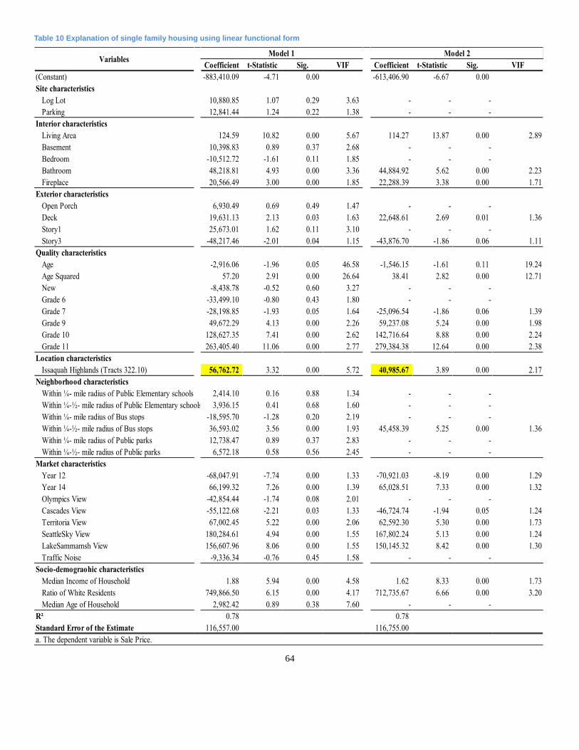
64

Table 10 Explanation of single family housing using linear functional form

Coefficient t-Statistic Sig. VIF Coefficient t-Statistic Sig. VIF

(Constant) -883,410.09 -4.71 0.00 -613,406.90 -6.67 0.00

Site characteristics

Log Lot 10,880.85 1.07 0.29 3.63 - - -

Parking 12,841.44 1.24 0.22 1.38 - - -

Interior characteristics

Living Area 124.59 10.82 0.00 5.67 114.27 13.87 0.00 2.89

Basement 10,398.83 0.89 0.37 2.68 - - -

Bedroom -10,512.72 -1.61 0.11 1.85 - - -

Bathroom 48,218.81 4.93 0.00 3.36 44,884.92 5.62 0.00 2.23

Fireplace 20,566.49 3.00 0.00 1.85 22,288.39 3.38 0.00 1.71

Exterior characteristics

Open Porch 6,930.49 0.69 0.49 1.47 - - -

Deck 19,631.13 2.13 0.03 1.63 22,648.61 2.69 0.01 1.36

Story1 25,673.01 1.62 0.11 3.10 - - -

Story3 -48,217.46 -2.01 0.04 1.15 -43,876.70 -1.86 0.06 1.11

Quality characteristics

Age -2,916.06 -1.96 0.05 46.58 -1,546.15 -1.61 0.11 19.24

Age Squared 57.20 2.91 0.00 26.64 38.41 2.82 0.00 12.71

New -8,438.78 -0.52 0.60 3.27 - - -

Grade 6 -33,499.10 -0.80 0.43 1.80 - - -

Grade 7 -28,198.85 -1.93 0.05 1.64 -25,096.54 -1.86 0.06 1.39

Grade 9 49,672.29 4.13 0.00 2.26 59,237.08 5.24 0.00 1.98

Grade 10 128,627.35 7.41 0.00 2.62 142,716.64 8.88 0.00 2.24

Grade 11 263,405.40 11.06 0.00 2.77 279,384.38 12.64 0.00 2.38

Location characteristics

Issaquah Highlands (Tracts 322.10) 56,762.72 3.32 0.00 5.72 40,985.67 3.89 0.00 2.17

Neighborhood characteristics

Within ¼ - mile radius of Public Elementary schools 2,414.10 0.16 0.88 1.34 - - -

Within ¼ -½ - mile radius of Public Elementary schools 3,936.15 0.41 0.68 1.60 - - -

Within ¼ - mile radius of Bus stops -18,595.70 -1.28 0.20 2.19 - - -

Within ¼ -½ - mile radius of Bus stops 36,593.02 3.56 0.00 1.93 45,458.39 5.25 0.00 1.36

Within ¼ - mile radius of Public parks 12,738.47 0.89 0.37 2.83 - - -

Within ¼ -½ - mile radius of Public parks 6,572.18 0.58 0.56 2.45 - - -

Market characteristics

Year 12 -68,047.91 -7.74 0.00 1.33 -70,921.03 -8.19 0.00 1.29

Year 14 66,199.32 7.26 0.00 1.39 65,028.51 7.33 0.00 1.32

Olympics View -42,854.44 -1.74 0.08 2.01 - - -

Cascades View -55,122.68 -2.21 0.03 1.33 -46,724.74 -1.94 0.05 1.24

Territoria View 67,002.45 5.22 0.00 2.06 62,592.30 5.30 0.00 1.73

SeattleSky View 180,284.61 4.94 0.00 1.55 167,802.24 5.13 0.00 1.24

LakeSammamsh View 156,607.96 8.06 0.00 1.55 150,145.32 8.42 0.00 1.30

Traffic Noise -9,336.34 -0.76 0.45 1.58 - - -

Socio-demograohic characteristics

Median Income of Household 1.88 5.94 0.00 4.58 1.62 8.33 0.00 1.73

Ratio of White Residents 749,866.50 6.15 0.00 4.17 712,735.67 6.66 0.00 3.20

Median Age of Household 2,982.42 0.89 0.38 7.60 - - -

R² 0.78 0.78

Standard Error of the Estimate 116,557.00 116,755.00

VariablesModel 1 Model 2

a. The dependent variable is Sale Price.

65

Table 11 Explanation of single family housing using semi-log functional form

Coefficient t-Statistic Sig. VIF Coefficient t-Statistic Sig. VIF

(Constant) 11.48 49.91 0.00 11.79 86.98 0.00

Site characteristics

Log Lot 0.03 2.64 0.01 3.63 0.02 2.05 0.04 2.75

Parking 0.05 3.81 0.00 1.38 0.05 4.23 0.00 1.25

Interior characteristics

Living Area 0.00 12.70 0.00 5.67 0.00 15.43 0.00 3.24

Basement 0.03 1.79 0.07 2.68 - - -

Bedroom 0.00 0.62 0.53 1.85 - - -

Bathroom 0.06 4.63 0.00 3.36 0.07 7.50 0.00 2.14

Fireplace 0.04 4.49 0.00 1.85 0.03 3.88 0.00 1.64

Exterior characteristics

Open Porch 0.02 1.85 0.06 1.47 - - -

Deck 0.03 2.59 0.01 1.63 0.04 3.40 0.00 1.40

Story1 0.02 0.90 0.37 3.10 - - -

Story3 -0.05 -1.84 0.07 1.15 - - -

Quality characteristics

Age 0.00 -1.69 0.09 46.58 - - -

Age Squared 0.00 2.14 0.03 26.64 0.00 1.46 0.14 3.47

New 0.02 0.84 0.40 3.27 - - -

Grade 6 -0.17 -3.36 0.00 1.80 -0.18 -3.71 0.00 1.65

Grade 7 -0.12 -6.48 0.00 1.64 -0.12 -7.00 0.00 1.56

Grade 9 0.07 5.04 0.00 2.26 0.08 5.67 0.00 2.06

Grade 10 0.15 6.85 0.00 2.62 0.17 8.70 0.00 2.18

Grade 11 0.24 8.26 0.00 2.77 0.26 9.49 0.00 2.45

Location characteristics

Issaquah Highlands (Tracts 322.10) 0.06 3.10 0.00 5.72 0.06 4.92 0.00 2.01

Neighborhood characteristics

Within ¼ - mile radius of Public Elementary schools -0.01 -0.44 0.66 1.34

Within ¼ -½ - mile radius of Public Elementary schools 0.01 0.68 0.50 1.60 - - -

Within ¼ - mile radius of Bus stops -0.01 -0.71 0.48 2.19 - - -

Within ¼ -½ - mile radius of Bus stops 0.05 3.59 0.00 1.93 0.06 5.62 0.00 1.35

Within ¼ - mile radius of Public parks 0.00 0.22 0.82 2.83 - - -

Within ¼ -½ - mile radius of Public parks 0.00 -0.01 0.99 2.45 - - -

Market characteristics

Year 12 -0.12 -11.39 0.00 1.33 -0.13 -11.83 0.00 1.29

Year 14 0.10 9.07 0.00 1.39 0.09 8.73 0.00 1.30

Olympics View -0.03 -1.08 0.28 2.01 - - -

Cascades View -0.08 -2.76 0.01 1.33 -0.09 -3.08 0.00 1.24

Territoria View 0.08 4.91 0.00 2.06 0.08 5.75 0.00 1.70

SeattleSky View 0.11 2.54 0.01 1.55 0.12 2.92 0.00 1.25

LakeSammamish View 0.12 4.97 0.00 1.55 0.10 4.70 0.00 1.31

Traffic Noise -0.03 -1.79 0.07 1.58 - - -

Socio-demograohic characteristics

Median Income of Household 0.00 6.06 0.00 4.58 0.00 8.07 0.00 1.87

Ratio of White Residents 0.51 3.38 0.00 4.17 0.37 2.88 0.00 3.11

Median Age of Household 0.00 0.51 0.61 7.60 - - -

R² 0.83 0.82

Standard Error of the Estimate 0.14 0.14

a. The dependent variable is Log Sale Price.

VariablesModel 1 Model 2

66

6.4 Discussion

By using two functional forms in a hedonic pricing model, this study estimates the premium or

discount that consumers are willing to pay for houses in Issaquah Highlands and in surrounding

conventional subdivisions. Additionally, this study determines whether there is a premium for

each characteristic.

First, a New Urbanism community in Issaquah Highlands confers appreciable housing value

benefits to a single family house. As expected, the coefficient of the binary variable indicating a

proxy for New Urbanism is positive and statistically significant, meaning that consumers are

willing to pay a $40,985-$56,762 (approximately 6.2-6.5 percent) premium for houses in

Issaquah Highlands.

In relation to interior, exterior, and quality characteristics for housing, this study shows that

consumers might pay a premium regardless of the number of bedrooms, because the number of

bedroom does not have a meaningful value in a limited living area. Also, consumers tend to

prefer to live in a one-story home than a two-story home, and a two-story home than a three-

story home. This is because homeowners are willing to pay a premium for a one-story home, and

a discount for a three-story home with reference point of a two-story home.

In particular, a grade representing construction quality acts as one of the most impactful factors

on single family housing values. A grade of 6 and 7 (below average) indicates a negative effect

on housing values relative to a grade 8 (Average). In addition, grades 9, 10, and 11 have a

significantly positive effect on housing values. However, the New variable is counter to the prior

67

expectation. Even though a New variable is not statistically significant, it indicates a negative

signal toward housing values.

Of the neighborhood characteristics, contrary to the expectation, this study reports that only

houses within a ¼ -½ -mile radius of Bus stops have a premium relative to the others. Based on

this result, houses within a ¼ -mile radius of Bus stops might not be preferred due to issues such

noise, dirt, and traffic. The other variables reveal that they do not satisfy a statistical significance,

though some have a positive effect on housing values.

Market characteristics have a significant effect on single family housing values. In particular,

there has been approximately 10 percent appreciation per year during the three-year period under

consideration. According to the Home Price Index (HPI)15

by the Federal Housing Finance

Agency, Seattle-Bellevue-Everett MSA reports that there were the 212 of HPI in 2012, the 243

of HPI in 2013, and the 263 of HPI in 2014 (FHFA 2015). These numbers reflects the rationality

of around 10 percent appreciation in the City of Issaquah. Also, views have a significant effect

on housing values. However, contrary to our expectation, Olympics and Cascade views do not

have a positive effect on housing values.

Finally, the effects of a neighborhood’s income level (Median Income of Household) and a

neighborhood’s racial composition (Ratio of White residents) are positive on housing values with

less P-value than 0.05.

15

For more information associated with the Federal Housing Finance Agency, refer to the website of the Federal

Housing Finance Agency at http://www.fhfa.gov/.

68

Chapter 7 Conclusion

The present study conducts the hedonic pricing analysis through two functional forms. The first

research model (linear form) reveals that a binary variable representing New Urbanism indicates

that people are willing to pay a $40,985-$56,762 premium for houses in Issaquah Highlands. The

second model (semi-log form) presents that a binary variable representing New Urbanism

indicates that people are willing to pay approximately a 6.2-6.5 percent premium for houses in

Issaquah Highlands.

Based on the results of two models, the findings from this study reveal that consumers are

willing to pay a premium to reside in a community developed according to New Urbanism

principles. These findings are valuable to urban planners, developers, policy makers, and

consumers, though the results are limited to only a single family dwelling in the City of Issaquah.

This study has several limitations. First, the 1,075 samples used in this study might lead to biased

results due to the small number of samples. The 1,075 sale transactions over the period January

2012 through December 2014, after omitting unusual observations, might not be very compelling.

If future studies are based on a greater number of observations, they might generate more

instructive results. As another alternative, if other New Urbanist communities as well as Issaquah

Highlands are analyzed together, more observations from several cases might help make the

analysis more robust and compelling.

Second, other limitations of the analysis include the fact that this study does not contain certain

variables by measuring and quantifying New Urbanism principles. Even though the present study

69

attempts to reflect as many housing attributes as are provided, adding the quantified New

Urbanism principles such as street design, circulation systems, and mixed land use will help

define the effects of New Urbanism on housing values more effectively.

Finally, this research used some census data sets at a tract level for Socio-demographic

characteristics. However, the data sets at a block- or a block group-level will produce more

accurate results and draw more persuasive conclusions.

Despite these limitations, the findings provide some useful insights about New Urbanism. The

present study provides several implications for future research and policy development in the

urban planning field. Further, even though it is difficult to predict the price of a single family

house, the statistical relationships among 1,075 sale prices and several characteristics are still

appealing and compelling, particularly for the City of Issaquah.

In the future, additional research should be conducted by investigating several other communities

of New Urbanism. These studies need to measure and quantify specific characteristics of New

Urbanism that contribute to housing values, based on a greater number of observations.

70

References

Alonso, William. 1964. "Location and land use. Toward a general theory of land rent." Location

and land use. Toward a general theory of land rent.

Bae, Chang-Hee Christine, Myung-Jin Jun, and Hyeon Park. 2003. "The impact of Seoul's

subway Line 5 on residential property values." Transport policy no. 10 (2):85-94.

Bae, Chang, Gail Sandlin, Alon Bassok, and Sungyop Kim. 2007. "The exposure of

disadvantaged populations in freeway air-pollution sheds: a case study of the Seattle and

Portland regions." ENVIRONMENT AND PLANNING B PLANNING AND DESIGN no.

34 (1):154.

Bohl, Charles C. 2000. "New urbanism and the city: Potential applications and implications for

distressed inner‐city neighborhoods."

Bowes, David R, and Keith R Ihlanfeldt. 2001. "Identifying the impacts of rail transit stations on

residential property values." Journal of Urban Economics no. 50 (1):1-25.

Box, George EP, and David R Cox. 1964. "An analysis of transformations." Journal of the Royal

Statistical Society. Series B (Methodological):211-252.

Boyle, Austin, Charles Barrilleaux, and Daniel Scheller. 2014. "Does Walkability Influence

Housing Prices?" Social Science Quarterly no. 95 (3):852-867.

Cervero, Robert, and Michael Duncan. 2002. "Land value impacts of rail transit services in San

Diego County." Report prepared for National Association of Realtors Urban Land

Institute.

Cervero, Robert, and Chang Deok Kang. 2011. "Bus rapid transit impacts on land uses and land

values in Seoul, Korea." Transport Policy no. 18 (1):102-116.

Clapp, John M, and Carmelo Giaccotto. 1992. "Estimating price indices for residential property:

a comparison of repeat sales and assessed value methods." Journal of the American

Statistical Association no. 87 (418):300-306.

CNU, Congress for the New Urbanism. 2015. CNU History 2015 [cited 02/12 2015]. Available

from https://www.cnu.org/history.

Cropper, Maureen L, Leland B Deck, and Kenenth E McConnell. 1988. "On the choice of

funtional form for hedonic price functions." The Review of Economics and Statistics:668-

675.

Duncan, Michael. 2010. "The impact of transit-oriented development on housing prices in San

Diego, CA." Urban studies.

Eppli, M.J., and C.C. Tu. 1999. Valuing the New Urbanism: The Impact of the New Urbanism on

Prices of Single-family Homes: Urban Land Institute.

FHFA, 2015 Federal Housing Finance Agency. 2015. House Price Index 2015 [cited 04/10 2015].

Available from http://www.fhfa.gov/DataTools/Downloads/Pages/House-Price-

Index.aspx.

Frank, Lawrence D, and Gary Pivo. 1994. "Impacts of mixed use and density on utilization of

three modes of travel: single-occupant vehicle, transit, and walking." Transportation

research record:44-44.

Garde, Ajay M. 2004. "New urbanism as sustainable growth? A supply side story and its

implications for public policy." Journal of Planning Education and Research no. 24

71

(2):154-170.

Gilderbloom, John I, William W Riggs, and Wesley L Meares. 2015. "Does walkability matter?

An examination of walkability’s impact on housing values, foreclosures and crime."

Cities no. 42:13-24.

Google Maps. 2015. Issaquah Highlands 2015 [cited 04/20 2015]. Available from

https://www.google.com/maps/place/Issaquah+Highlands,+Issaquah,+WA/@47.544448,-

122.0106135,14z/data=!3m1!4b1!4m2!3m1!1s0x54906ff4702df4b1:0x8e1b3de73b7caf3

2.

Hammer, Thomas R, Robert E Coughlin, and Edward T Horn IV. 1974. "The effect of a large

urban park on real estate value." Journal of the American Institute of Planners no. 40

(4):274-277.

Hess, Daniel Baldwin, and Tangerine Maria Almeida. 2007. "Impact of proximity to light rail

rapid transit on station-area property values in Buffalo, New York." Urban studies no. 44

(5-6):1041-1068.

IH, Issaquah Highlands. 2015. Community Guiding Principles 2015 [cited 02/25 2015].

Available from http://www.issaquahhighlands.com/learn/about-issaquah-highlands/.

Irwin, Elena G. 2002. "The effects of open space on residential property values." Land

economics no. 78 (4):465-480.

Janssen, Christian, and Bo Söderberg. 1999. "Estimating market prices and assessed values for

income properties." Urban Studies no. 36 (2):359-376.

Kang, Chang Deok, and Robert Cervero. 2009. "From elevated freeway to urban greenway: land

value impacts of the CGC project in Seoul, Korea." Urban Studies no. 46 (13):2771-2794.

Knaap, Gerrit J, Chengr Ding, and Lewis D Hopkins. 2001. "Do plans matter? The effects of

light rail plans on land values in station areas." Journal of Planning Education and

Research no. 21 (1):32-39.

Knaap, Gerrit, and Emily Talen. 2005. "New urbanism and smart growth: a few words from the

academy." International Regional Science Review no. 28 (2):107-118.

Linneman, Peter. 1980. "Some empirical results on the nature of the hedonic price function for

the urban housing market." Journal of Urban Economics no. 8 (1):47-68.

Litman, Todd. 2004. "Economic value of walkability." World Transport Policy & Practice no. 10

(1):5-14.

Malpezzi, Stephen. 2003. "Hedonic pricing models: a selective and applied review." Section in

Housing Economics and Public Policy: Essays in Honor of Duncan Maclennan.

NAR, National Association of REALTORS. 2015. NAR 2013 Community Preference Survey

2013 [cited 02/20 2015]. Available from

http://www.realtor.org/sites/default/files/reports/2013/2013-community-preference-press-

release.pdf.

NU, New Urbanism. 2015. PRINCIPLES OF URBANISM 2015 [cited 05/30 2015]. Available

from http://www.newurbanism.org/newurbanism/principles.html.

Randall, Guttery S. 2002. "The effects of subdivision design on housing values: the case of

alleyways." Journal of Real Estate Research no. 23 (3):265-274.

Rosen, Sherwin. 1974. "Hedonic prices and implicit markets: product differentiation in pure

competition." The journal of political economy:34-55.

72

Skaburskis, Andrejs. 2006. "New Urbanism and Sprawl A Toronto Case Study." Journal of

Planning Education and Research no. 25 (3):233-248.

Smith, Neil. 2002. "New globalism, new urbanism: gentrification as global urban strategy."

Antipode no. 34 (3):427-450.

Sohn, Dong Wook, Anne Vernez Moudon, and Jeasun Lee. 2012. "The economic value of

walkable neighborhoods." Urban Design International no. 17 (2):115-128.

Song, Yan, and Gerrit-Jan Knaap. 2003. "New urbanism and housing values: a disaggregate

assessment." Journal of Urban Economics no. 54 (2):218-238.

Song, Yan, and Gerrit-Jan Knaap. 2004. "Measuring the effects of mixed land uses on housing

values." Regional Science and Urban Economics no. 34 (6):663-680.

Steuteville, Robert. 2000. "The New Urbanism: An alternative to modern, automobile-oriented

planning and development." New Urban News:1-6.

Tu, Charles C, and Mark J Eppli. 2001. "An empirical examination of traditional neighborhood

development." Real Estate Economics no. 29 (3):485-501.

Washington, Emily. 2013. "Role of walkability in driving home values." Leadership and

Management in Engineering no. 13 (3):123-130.

Yan, Sisi, Eric Delmelle, and Mike Duncan. 2012. "The impact of a new light rail system on

single-family property values in Charlotte, North Carolina." Journal of Transport and

Land Use no. 5 (2).

Zou, Kelly H, Kemal Tuncali, and Stuart G Silverman. 2003. "Correlation and simple linear

regression 1." Radiology no. 227 (3):617-628.

73

Appendix: House Price Index by Federal Housing Finance Agency

Metropolitan Year Quarter Index

Seattle-Bellevue-Everett, WA (MSAD) 2000 1 157.08Seattle-Bellevue-Everett, WA (MSAD) 2000 2 160.44Seattle-Bellevue-Everett, WA (MSAD) 2000 3 162.07Seattle-Bellevue-Everett, WA (MSAD) 2000 4 163.43Seattle-Bellevue-Everett, WA (MSAD) 2001 1 167.62Seattle-Bellevue-Everett, WA (MSAD) 2001 2 170.43Seattle-Bellevue-Everett, WA (MSAD) 2001 3 172.75Seattle-Bellevue-Everett, WA (MSAD) 2001 4 172.91Seattle-Bellevue-Everett, WA (MSAD) 2002 1 175.19Seattle-Bellevue-Everett, WA (MSAD) 2002 2 179.58Seattle-Bellevue-Everett, WA (MSAD) 2002 3 181.1Seattle-Bellevue-Everett, WA (MSAD) 2002 4 182.33Seattle-Bellevue-Everett, WA (MSAD) 2003 1 185.14Seattle-Bellevue-Everett, WA (MSAD) 2003 2 189.7Seattle-Bellevue-Everett, WA (MSAD) 2003 3 192.28Seattle-Bellevue-Everett, WA (MSAD) 2003 4 195.24Seattle-Bellevue-Everett, WA (MSAD) 2004 1 200.87Seattle-Bellevue-Everett, WA (MSAD) 2004 2 207.82Seattle-Bellevue-Everett, WA (MSAD) 2004 3 212.66Seattle-Bellevue-Everett, WA (MSAD) 2004 4 218.67Seattle-Bellevue-Everett, WA (MSAD) 2005 1 226.87Seattle-Bellevue-Everett, WA (MSAD) 2005 2 238.3Seattle-Bellevue-Everett, WA (MSAD) 2005 3 250.17Seattle-Bellevue-Everett, WA (MSAD) 2005 4 253.5Seattle-Bellevue-Everett, WA (MSAD) 2006 1 265.07Seattle-Bellevue-Everett, WA (MSAD) 2006 2 278Seattle-Bellevue-Everett, WA (MSAD) 2006 3 287.3Seattle-Bellevue-Everett, WA (MSAD) 2006 4 289.6Seattle-Bellevue-Everett, WA (MSAD) 2007 1 296.78Seattle-Bellevue-Everett, WA (MSAD) 2007 2 303.81Seattle-Bellevue-Everett, WA (MSAD) 2007 3 304.64Seattle-Bellevue-Everett, WA (MSAD) 2007 4 299.45Seattle-Bellevue-Everett, WA (MSAD) 2008 1 290.71Seattle-Bellevue-Everett, WA (MSAD) 2008 2 288.35Seattle-Bellevue-Everett, WA (MSAD) 2008 3 279.11Seattle-Bellevue-Everett, WA (MSAD) 2008 4 265.57Seattle-Bellevue-Everett, WA (MSAD) 2009 1 258.91Seattle-Bellevue-Everett, WA (MSAD) 2009 2 251.32Seattle-Bellevue-Everett, WA (MSAD) 2009 3 245.63Seattle-Bellevue-Everett, WA (MSAD) 2009 4 248.47Seattle-Bellevue-Everett, WA (MSAD) 2010 1 242.59Seattle-Bellevue-Everett, WA (MSAD) 2010 2 244.39Seattle-Bellevue-Everett, WA (MSAD) 2010 3 237.19Seattle-Bellevue-Everett, WA (MSAD) 2010 4 225.11Seattle-Bellevue-Everett, WA (MSAD) 2011 1 221.41Seattle-Bellevue-Everett, WA (MSAD) 2011 2 219.9Seattle-Bellevue-Everett, WA (MSAD) 2011 3 216.46Seattle-Bellevue-Everett, WA (MSAD) 2011 4 207.01Seattle-Bellevue-Everett, WA (MSAD) 2012 1 211.52Seattle-Bellevue-Everett, WA (MSAD) 2012 2 223.87Seattle-Bellevue-Everett, WA (MSAD) 2012 3 230.03Seattle-Bellevue-Everett, WA (MSAD) 2012 4 237.78Seattle-Bellevue-Everett, WA (MSAD) 2013 1 243Seattle-Bellevue-Everett, WA (MSAD) 2013 2 255.49Seattle-Bellevue-Everett, WA (MSAD) 2013 3 265.14Seattle-Bellevue-Everett, WA (MSAD) 2013 4 261.24Seattle-Bellevue-Everett, WA (MSAD) 2014 1 262.79Seattle-Bellevue-Everett, WA (MSAD) 2014 2 277.79Seattle-Bellevue-Everett, WA (MSAD) 2014 3 278.89Seattle-Bellevue-Everett, WA (MSAD) 2014 4 279.94