The Impact of Stellar Variability on yKepler’s Search for Transiting Planets

Jessie Christiansen

Kepler Participating ScientistNASA Exoplanet Science Institute/CaltechNASA Exoplanet Science Institute/Caltech

jessie.christiansen@caltech.edu

With thanks to collaborators:Chris Burke, Bruce Clarke, Natalie Batalha,

Page 1

Mike Haas, Shawn Seader, and the Kepler team

Thinking about stellar noise, pre-Kepler

Problem of correlated ‘red’ noise (non stationary non Gaussian) impactingo Problem of correlated red noise (non-stationary, non-Gaussian) impacting transit searches long identified (Borucki, Scargle & Hudson 1985).

o Based on extrapolation based on noise measured in the Sun, and assumptions about the Sun relative to other ‘typical’ stars - Jenkins et al. (2002), Batalha et al. (2002)

o Photometric precision of 20 ppm in 6.5 hours on Vmag = 12 solar-like star

o Considerable effort in the early 2000’s to develop a two-step detection algorithm for transits that included stellar variability filters, e.g. Jenkins et al. (2002) Ai i & I i (2004) d f th i(2002), Aigrain & Irwin (2004) and references therein

o Also, identification of interesting stellar types (non-FGK main sequence , g yp ( qstars) with their own intrinsic variability

o White dwarfs (Farmer & Agol, 2003)Giant stars (Assef Gaudi & Stanek 2009)

Page 4

o Giant stars (Assef, Gaudi & Stanek, 2009)

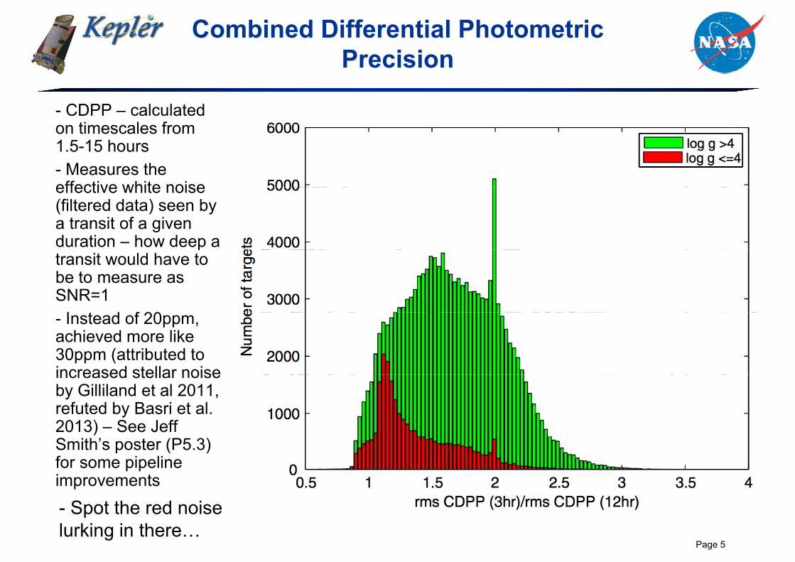
Combined Differential Photometric PrecisionPrecision

- CDPP – calculated ti l fon timescales from

1.5-15 hours- Measures the effective white noiseeffective white noise (filtered data) seen by a transit of a given duration – how deep a

4000-7000K

ptransit would have to be to measure as SNR=1

I d f 20 4000-7000K- Instead of 20ppm, achieved more like 30ppm (attributed to increased stellar noise

>4.0increased stellar noise by Gilliland et al 2011, refuted by Basri et al. 2013) – See Jeff Smith’s poster (P5.3) for some pipeline improvements

Page 5

Christiansen et al 2012- Spot the red noise lurking in there…

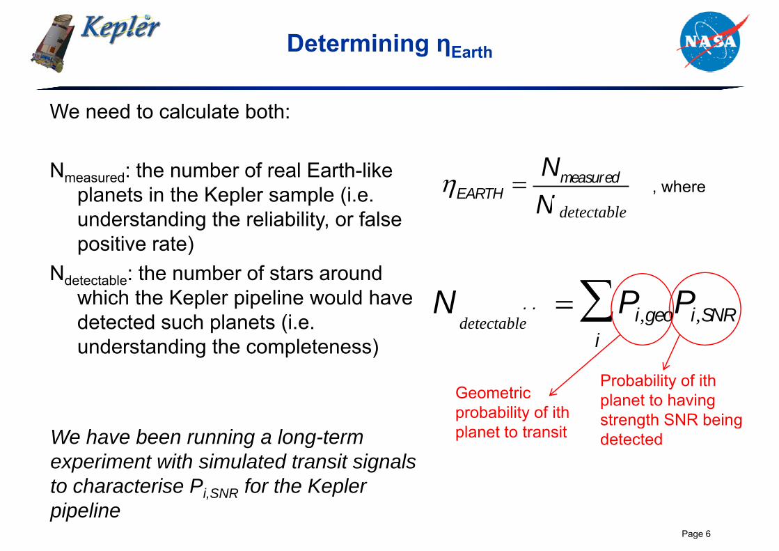
Determining ηEarth

We need to calculate both:

Nmeasured: the number of real Earth-like Nmeasured hereplanets in the Kepler sample (i.e. understanding the reliability, or false positive rate)

EARTH Nmeasurabledetectable

, where

positive rate)Ndetectable: the number of stars around

which the Kepler pipeline would have N P Pp p pdetected such planets (i.e. understanding the completeness)

Nmeasurable Pi,geoPi,SNRi

detectable

Geometric probability of ith

l t t t it

Probability of ith planet to having strength SNR being

planet to transitg g

detectedWe have been running a long-term experiment with simulated transit signals to characterise Pi SNR for the Kepler

Page 6

to characterise Pi,SNR for the Kepler pipeline

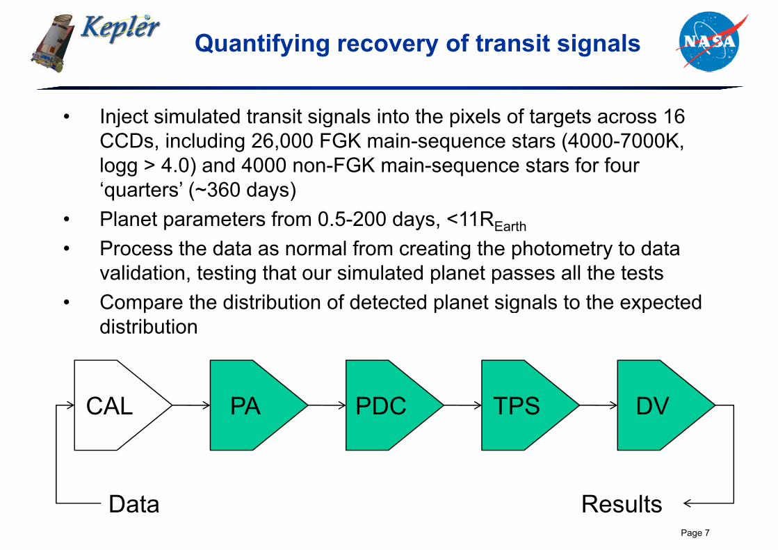
Quantifying recovery of transit signals

• Inject simulated transit signals into the pixels of targets across 16Inject simulated transit signals into the pixels of targets across 16 CCDs, including 26,000 FGK main-sequence stars (4000-7000K, logg > 4.0) and 4000 non-FGK main-sequence stars for four ‘ t ’ ( 360 d )‘quarters’ (~360 days)

• Planet parameters from 0.5-200 days, <11REarth

P th d t l f ti th h t t t d t• Process the data as normal from creating the photometry to data validation, testing that our simulated planet passes all the tests

• Compare the distribution of detected planet signals to the expectedCompare the distribution of detected planet signals to the expected distribution

PA PDC TPS DVCAL

Page 7

Data Results

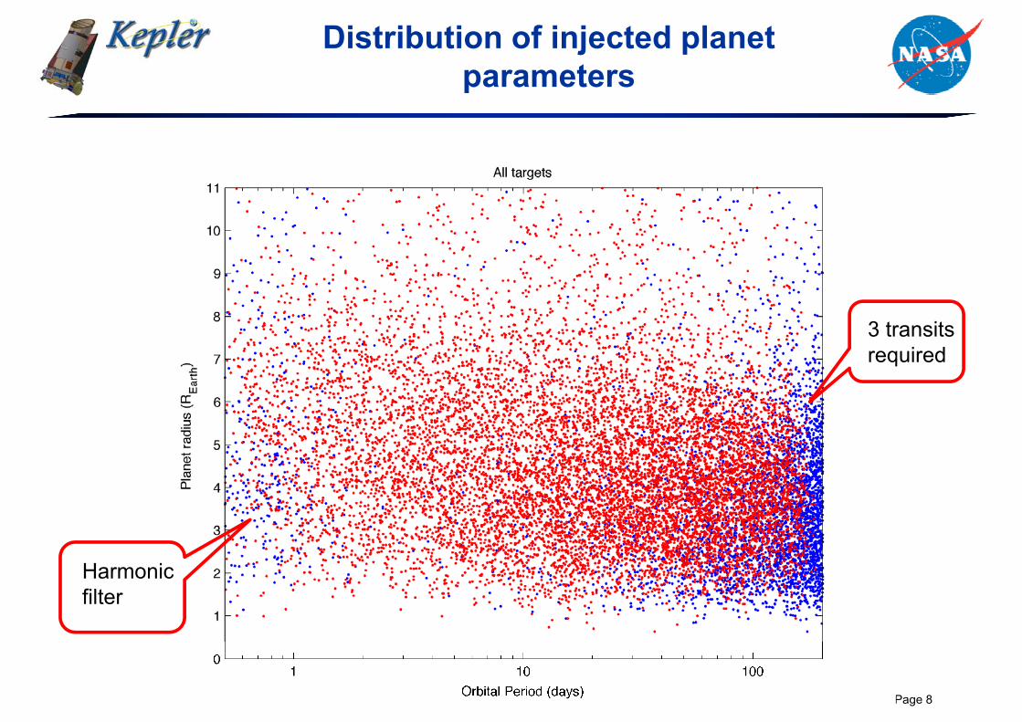
Distribution of injected planet parametersparameters

3 transits required

Harmonicfilter

Page 8

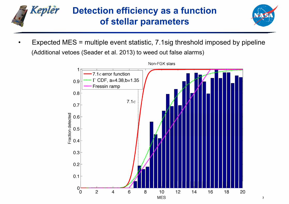
Detection efficiency as a function of stellar parametersof stellar parameters

• Expected MES = multiple event statistic, 7.1sig threshold imposed by pipelinep p , g p y p p(Additional vetoes (Seader et al. 2013) to weed out false alarms)

Page 9

What is happening to the transit signals?

• Signal masking in (correlated) noisy data

• Examine non-detections of injections with expected MES > 10• Non-FGK: 2.67 candidate per target when injection not recovered (vs. 1.16) • (FGK: 1.16 candidates per target when injection not recovered (vs. 1.12))(FGK: 1.16 candidates per target when injection not recovered (vs. 1.12))• This effects the window function/duty cycle (number of searchable cadences)

(N.B. impact for multi-planet systems…)

• Another possible loss may be in the vetoes (Seader et al. 2013)• In addition to the 7.1σ threshold, apply a set of χ2 discriminators to

remove false alarms still need to look at for quiet vs variable starsremove false alarms - still need to look at for quiet vs. variable stars

Page 10

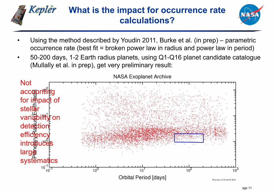
What is the impact for occurrence rate calculations?calculations?

• Using the method described by Youdin 2011, Burke et al. (in prep) – parametric g y , ( p p) poccurrence rate (best fit = broken power law in radius and power law in period)

• 50-200 days, 1-2 Earth radius planets, using Q1-Q16 planet candidate catalogue (Mullally et al in prep) get very preliminary result:(Mullally et al. in prep), get very preliminary result:

Not accounting for impact of stellarstellar variability on detection efficiency introduces largelarge systematics

Page 11

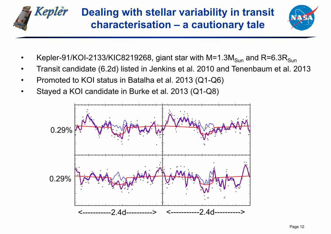
Dealing with stellar variability in transit characterisation – a cautionary talecharacterisation a cautionary tale

• Kepler-91/KOI-2133/KIC8219268, giant star with M=1.3MSun and R=6.3RSun

• Transit candidate (6.2d) listed in Jenkins et al. 2010 and Tenenbaum et al. 2013P t d t KOI t t i B t lh t l 2013 (Q1 Q6)• Promoted to KOI status in Batalha et al. 2013 (Q1-Q6)

• Stayed a KOI candidate in Burke et al. 2013 (Q1-Q8)

0 29%0.29%

0.29%

Page 12

<-----------2.4d----------> <-----------2.4d---------->

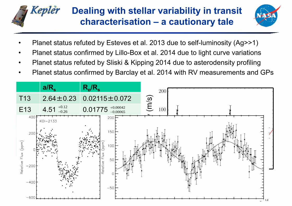
Dealing with stellar variability in transit characterisation – a cautionary talecharacterisation a cautionary tale

• Planet status refuted by Esteves et al. 2013 due to self-luminosity (Ag>>1)y y ( g )• Planet status confirmed by Lillo-Box et al. 2014 due to light curve variations• Planet status refuted by Sliski & Kipping 2014 due to asterodensity profiling• Planet status confirmed by Barclay et al. 2014 with RV measurements and GPs

a/Rs Rp/Rs

T13 2.64±0.23 0.02115±0.072E13 4.51 0.01775 0.00065

0.000420.260.12

L14 2.36 0.02255K14 4.476 0.019429

0.350.10

0.0970.031

0.0000660.000109

0.1180.023

B14 2.463±0.11

0.0212±0.000034

Page 13

Going forward…

• Account for stellar variability/noise in occurrence rate considerations!• Increased stellar noise increases the required SNRq• AND makes detection more difficult at the same SNR

• Account for stellar variability/noise in transit characterisation!• Different treatments of the stellar noise

= different transit depths/durations = different planet parameters= different planet parameters= different planet interpretations!

• Keep playing with Kepler data!• New candidates and pipeline products coming soon

Page 14