Embed Size (px)
Citation preview
INTERNATIONAL JOURNAL OF ENVIRONMENTAL SCIENCES Volume 3, No 6, 2013
© Copyright by the authors - Licensee IPA- Under Creative Commons license 3.0
Research article ISSN 0976 – 4402
Received on January 2013 Published on August 2013 2323
The impact of temperature on mortality in Ludhiana City, India: A time
series analysis Suresh Kumar Sharma1, Rajesh Kumar2, Rashmi Aggarwal1, PVM Lakshmi2, Kanchan Jain1
1- Department of Statistics, Panjab University, Chandigarh, India
2- School of Public Health, Post Graduate Institute of Medical Education and Research,
Chandiagrh, India
doi:10.6088/ijes.2013030600048
ABSTRACT
The widely used generalized additive model (GAM) is a flexible and effective technique for
conducting non-linear regression analysis in time-series studies. There is strong evidence that
episodes of extremely hot or cold temperatures are associated with increased mortality in
many parts of the world. Time series designs are extremely useful to examine association
between daily apparent temperature and daily mortality counts. Hence, the effect of
temperature on mortality was studied in Ludhiana city of Punjab in Northern India. As a part
of the Health Effects Institute (HEI), Boston USA, project, Meteorological and mortality data
was obtained for the years 2002-2004. Sahnewal Airport in Ludhiana City records
temperature, dew point, wind speed and relative humidity at 8.30 AM, 11.30 AM, and 5.30
PM. Daily death records were obtained from the civil registration system in Ludhiana. The
association between temperature and mortality was established using the generalized additive
model (GAM) with penalized spline smoothers at 8,4,4 degrees of freedom (df) in R software
with mortality count (excluding accidents) as a dependent variable. Smoothers for day of the
week, relative humidity and wind speed were included in the model. With rapid
industrialization and extreme temperature variations in Ludhiana city, the temperature was
significantly associated with mortality. Sensitivity analysis shows that elderly (>65 years)
population was much affected with temperature variations, particularly, during winter season.
The study shows there is need to improve the overall registration system of deaths. Cause
specific analysis was not possible as cause of death was not clearly mentioned in most of the
deaths.
Keywords: Generalized additive model, relative humidity, windspeed, mortality, sensitivity
analysis, time series analysis.
1. Introduction
For many years, the effect of temperature on mortality has been the subject of numerous
studies, mostly examining the impact of extreme weather events (Hastie and Tibshirani,1990
and Ha et al.,2011). Numerous studies have shown a positive association between daily
mortality and temperature during extreme hot and cold weather. Early studies found a relation
between peak of daily mortality and a concomitantly peak of temperatures (Carson et al.,2006
and Kim et al.,2006). Mortality due to extreme temperatures have also been reported by many
authors (Braga et al.,2001). In these studies, the elderly and those suffering from underlying
medical conditions such as circulatory and respiratory diseases were found to be more
vulnerable (Hajat et al,2002 and Goldberg et al.,2011). Most of the existing research has been
conducted in Europe (McKee,1989, Baker,2008 and Ballester et al.,2011), Spain (Ballester et
The impact of temperature on mortality in Ludhiana City, India: A time series analysis
Suresh Kumar Sharma et al International Journal of Environmental Sciences Volume 3 No.6 2013
2324
al.,1997), Dutch (Huynen,2001), Germany (Hoffmann,2008), Canada (Goldberg et al.,2011)
and America (Ellis and Nelson,1978, Curriero,2002, Anderson and Bell,2009, Ostro et
al.,2009 and Basu and Malig,2011). Very few studies in Asia, South Korea (McKee,1989 and
Ha et al.,2011), India (Kumar et al.,2010) which is rapidly developing and where effects of
temperature on mortality are increasing have been conducted. The effect of various
temperature indicators on different mortality categories in a subtropical city of Brisbane have
also been conducted recently (Yu et al.,2011). Reviews of epidemiologic studies from 2001
to 2008 have been conducted by Basu (Basu,2006). Modelling temperature effects on
mortality using multiple segmented relationships with common break points was also
conducted (Muggeo,2008).
Time Series analysis using Generalized Additive Model (GAM) (Hastie and Tibshirani,1990)
show an association between temperature and mortality across a range of less extreme
temperatures after smoothing the effects of day of the week, relative humidity and wind
speed. In this paper, the authors describes the temperature-mortality association for year
2002-2004 in Ludhiana City of northern India by estimating the relative risks of mortality
using GAM with quasi-poisson function for mortality due to natural causes (excluding
accidents) as the dependent variable and temperature as the independent variable with
penalized spline smoothers for day of the week, relative humidity and wind speed. Current
and recent day’s temperatures were the weather components most strongly predictive of
mortality, and mortality risk generally decreased as temperate increased from the coldest days
to a certain threshold temperature, above which mortality risk increased as temperature
increased to highest level or decreased to the lowest level. The model developed in this
analysis is potentially useful for projecting the consequences of climate change scenarios and
offering insights into susceptibility to the adverse effects of temperature.
2. Material and methods
The present study was carried out in Ludhiana city, which is the largest city of Punjab in
northern India. The Indian meteorological Department, New Delhi, records meteorological
data at the Sahnewal airport of Ludhiana city. Temperature, relative humidity, dew point,
wind speed and wind direction was recorded daily at 8.30 AM, 11.30 AM and 5.30 PM.
Meteorological data was available for all the 365 days in a year. Municipal corporation
records mortality data at two Centre’s which register deaths for zone A and B, C and D of the
city respectively. Government and Private hospitals report deaths that occur in their premises
and heads of families reports deaths which happen at home or places other than hospital to
the municipal corporation office in their respective zone. The data available in the registers
by registration number, name of the deceased, father’s name, age, sex, date of death, cause of
death, place of death and address of the deceased were entered in computer for analysis.
Standard operating procedures were developed for maintaining the quality of data. During
data entry, 2% of the entries were randomly compared with the records, each week in each of
the two zones. At the end of data entry, a 100% recheck was again carried out. It has been
found out that sex and age were not mentioned in 207(0.7%) and 21(0.1%) of the deaths.
2.1 Statistical analysis
The data was examined for quality and consistency. Summary statistics, mean, standard
deviation, minimum, maximum and range were computed as per Table1 for temperature,
relative humidity and wind speed. Overall in the 3 years period 2002-2004, 28007 deaths
were registered with an average of 25.4 deaths per day. The age-sex distribution of the deaths
The impact of temperature on mortality in Ludhiana City, India: A time series analysis
Suresh Kumar Sharma et al International Journal of Environmental Sciences Volume 3 No.6 2013
2325
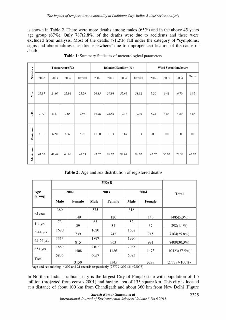
is shown in Table 2. There were more deaths among males (65%) and in the above 45 years
age group (67%). Only 787(2.8%) of the deaths were due to accidents and these were
excluded from analysis. Most of the deaths (71.2%) fall under the category of “symptoms,
signs and abnormalities classified elsewhere” due to improper certification of the cause of
death. Table 1: Summary Statistics of meteorological parameters
Sta
tist
ics Temperature(0C) Relative Humidity (%) Wind Speed (km/hour)
2002 2003 2004 Overall 2002 2003 2004 Overall 2002 2003 2004 Overa
ll
Mea
n
25.87 24.99 25.91 25.59 56.85 59.86 57.66 58.12 7.50 6.41 6.70 6.87
S.D
.
7.72 8.37 7.65 7.93 16.78 21.58 19.16 19.30 5.22 4.83 4.50 4.88
Min
imu
m
8.13 6.20 8.37 6.20 11.00 10.33 13.67 10.33 .00 .00 .00 .00
Ma
xim
um
41.53 41.47 40.60 41.53 93.67 99.67 97.67 99.67 42.67 35.67 27.33 42.67
Table 2: Age and sex distribution of registered deaths
Age
Group
YEAR
Total 2002 2003 2004
Male Female Male Female Male Female
<1year 380
149
375
120
318
143 1485(5.3%)
1-4 yrs 73
39 63
34 52
37 298(1.1%)
5-44 yrs 1680
739 1620
742 1668
715 7164(25.8%)
45-64 yrs 1313
815 1897
963 1990
931 8409(30.3%)
65+ yrs 1889
1408 2102
1486 2065
1473 10423(37.5%)
Total 5835
3150
6057
3345
6093
3299 27779*(100%) *age and sex missing in 207 and 21 records respectively (27779+207+21=28007)
In Northern India, Ludhiana city is the largest City of Punjab state with population of 1.5
million (projected from census 2001) and having area of 135 square km. This city is located
at a distance of about 100 km from Chandigarh and about 360 km from New Delhi (Figure
The impact of temperature on mortality in Ludhiana City, India: A time series analysis
Suresh Kumar Sharma et al International Journal of Environmental Sciences Volume 3 No.6 2013
2326
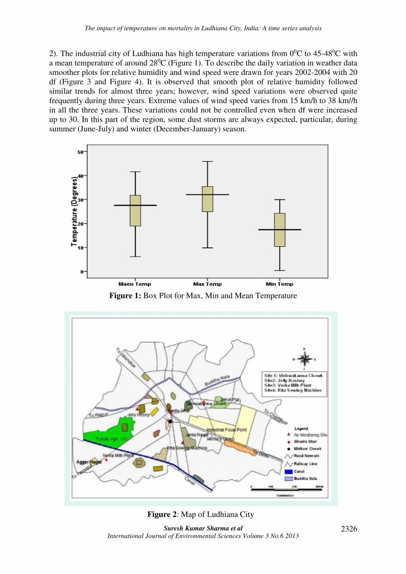
2). The industrial city of Ludhiana has high temperature variations from 00C to 45-480C with
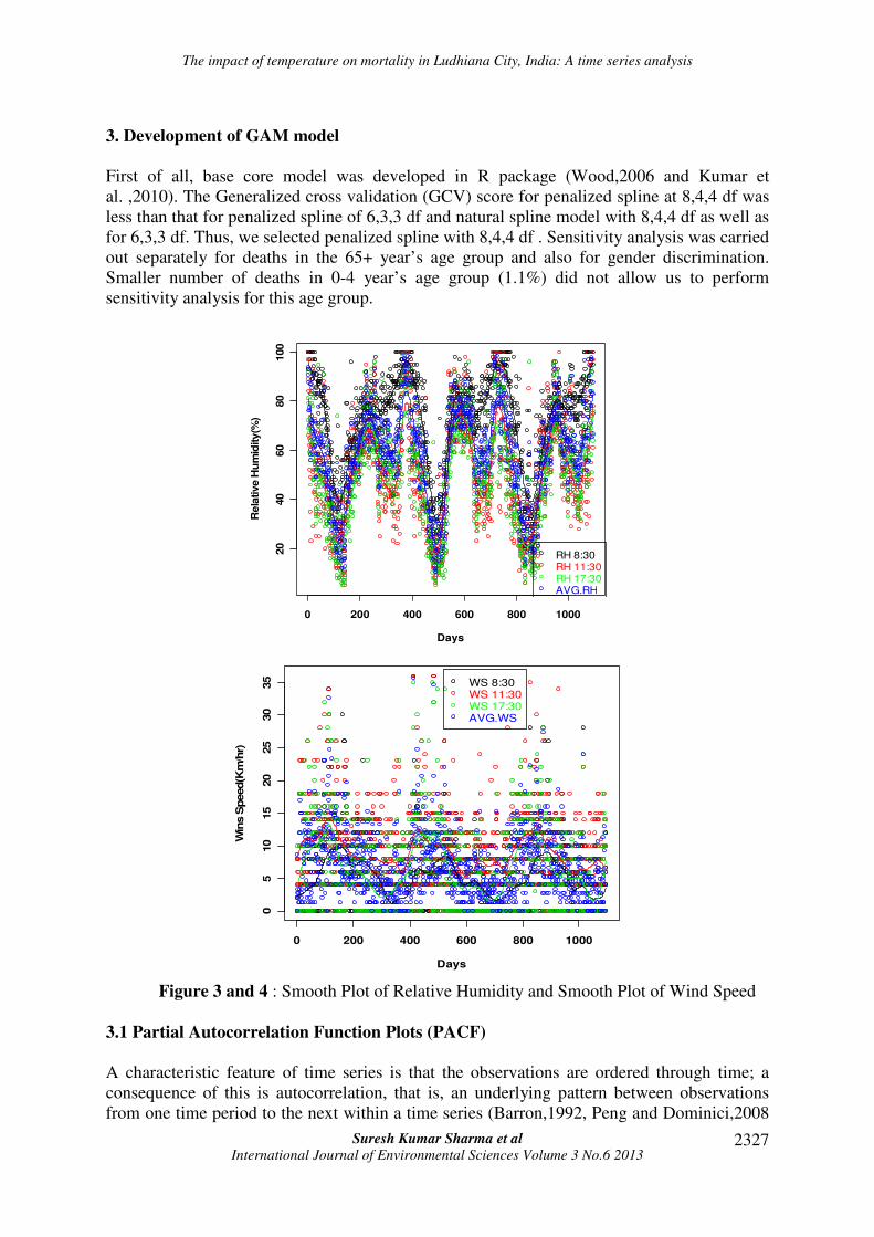
a mean temperature of around 280C (Figure 1). To describe the daily variation in weather data
smoother plots for relative humidity and wind speed were drawn for years 2002-2004 with 20
df (Figure 3 and Figure 4). It is observed that smooth plot of relative humidity followed
similar trends for almost three years; however, wind speed variations were observed quite
frequently during three years. Extreme values of wind speed varies from 15 km/h to 38 km//h
in all the three years. These variations could not be controlled even when df were increased
up to 30. In this part of the region, some dust storms are always expected, particular, during
summer (June-July) and winter (December-January) season.
Figure 1: Box Plot for Max, Min and Mean Temperature
Figure 2: Map of Ludhiana City
The impact of temperature on mortality in Ludhiana City, India: A time series analysis
Suresh Kumar Sharma et al International Journal of Environmental Sciences Volume 3 No.6 2013
2327
3. Development of GAM model
First of all, base core model was developed in R package (Wood,2006 and Kumar et
al. ,2010). The Generalized cross validation (GCV) score for penalized spline at 8,4,4 df was
less than that for penalized spline of 6,3,3 df and natural spline model with 8,4,4 df as well as
for 6,3,3 df. Thus, we selected penalized spline with 8,4,4 df . Sensitivity analysis was carried
out separately for deaths in the 65+ year’s age group and also for gender discrimination.
Smaller number of deaths in 0-4 year’s age group (1.1%) did not allow us to perform
sensitivity analysis for this age group.
0 200 400 600 800 1000
20
40
60
80
100
Days
Rela
tive H
um
idity(%
)
RH 8:30RH 11:30RH 17:30AVG.RH
0 200 400 600 800 1000
05
10
15
20
25
30
35
Days
Win
s S
peed(K
m/h
r)
WS 8:30WS 11:30WS 17:30AVG.WS
Figure 3 and 4 : Smooth Plot of Relative Humidity and Smooth Plot of Wind Speed
3.1 Partial Autocorrelation Function Plots (PACF)
A characteristic feature of time series is that the observations are ordered through time; a
consequence of this is autocorrelation, that is, an underlying pattern between observations
from one time period to the next within a time series (Barron,1992, Peng and Dominici,2008

The impact of temperature on mortality in Ludhiana City, India: A time series analysis
Suresh Kumar Sharma et al International Journal of Environmental Sciences Volume 3 No.6 2013
2328
and Ha et al., 2011). We can define autocorrelation at log k as the correlation between
observations k time periods apart. This can be estimated for lags k = 0, 1, 2 . . . as
where xt denotes the observation at time t and denotes the sample mean of the series .
The partial autocorrelation at lag k is defined as the partial correlation between observations k
time periods apart. That is, it is the correlation between xt and xt-k after taking out the effect
of the intervening observations xt-1, . . ., xt-k+1. It can be estimated using a fast computational
algorithm. The collection of autocorrelations at lags k = 1, 2, . . . is known as the
autocorrelation function (ACF). Similarly, the collection of partial autocorrelations is known
as the partial autocorrelation function (PACF).
3.2 Residual Plot
A residual plot is a graph that shows the residuals on the vertical axis and the independent
variable on the horizontal axis. If the points in a residual plot are randomly dispersed around
the horizontal axis, a linear regression model is appropriate for the data; otherwise, a non-
linear model is more appropriate. The difference between the observed value of the
dependent variable (y) and the predicted value (ŷ) is called the residual (e). Each data point
has one residual. Thus, Residual = Observed value - Predicted value. A plot of residuals
versus predicted response is essentially used to spot possible heteroscedasticity (non-constant
variance across the range of the predicted values), as well as influential observations
(possible outliers). Usually, we expect such plot to exhibit no particular pattern (a funnel-like
plot would indicate that variance increase with mean). Plotting residuals against one predictor
can be used to check the linearity assumption.
Since a GAM is just a penalized GLM, residual plots are checked, exactly as for a GLM. The
distribution of scaled residuals was examined, marginally, and plotted against covariates and
fitted values. In R residuals (model) extracts residuals and gam.check (model) produces
simple residual plots, and summary of convergence information.Plot (model, residuals =
TRUE) plots smooth terms with partial residuals overlaid. In the sequel, we have worked out
the PACF and Residual plots for Lag0, Lag1, Lag2 and Lag3 (Schwartz, 2000) along with
predicted plot of mortality in R using, PS(8,4,4) model.
3.2.1 Model: Effect of Temperature on Mortality: GeneralizedAdditive Model (GAM)
Log (E(mortality))=Temperature +s(day effect)+ s(relative humidity)+ s(wind speed)
1. Generalized Additive Model (GAM) with penalized spline smoothers in R.
2. Quasi-Poisson function with mortality from all natural causes as the dependent
variables
3. Smoothers for day effect, relative humidity and wind speed
4. Day of week terms (from Monday through Sunday).
5. Exposure at single-day lags of 0 to 3 days

The impact of temperature on mortality in Ludhiana City, India: A time series analysis
Suresh Kumar Sharma et al International Journal of Environmental Sciences Volume 3 No.6 2013
2329
Table 3: Effect of Temperature on Mortality in Ludhiana 2002-2004 (all deaths)
Mean temp 95% CI
Lag
Effects N β-Coeff.
Relative
Risk P-value Lower Upper
Lag 0 1096 0.015443 1.166992586 .0000118* 1.08945 1.25005
Lag 1 1095 0.011836 1.125649272 .0000421* 1.06391 1.19097
Lag 2 1094 0.007806 1.081187528 0.0048 * 1.02421 1.14133
Lag 3 1093 0.005579 1.057375612 0.0406 ** 1.00244 1.11532
* (p < .01), **(p < .05)
-20
2
Day
Re
sid
ua
l
Jan02 Jul02 Jan03 Jul03 Jan04 Jul04 Dec04
0 5 10 15 20 25 30
-0.1
00
.00
0.1
0
Lag
Pa
rtia
l A
CF
10
20
30
40
50
Day
Num
be
r o
f ep
isod
es
Jan02 Jul02 Jan03 Jul03 Jan04 Jul04 Dec04
Figure 5: Residual and PACF plots for PS (8,4,4) model along with predicted plot of
mortality (Lag0)
It is evident from PACF and Residual plots that there is significant effect of temperature on
mortality after smoothing the effects of day, relative humidity and wind speed. The predicted
The impact of temperature on mortality in Ludhiana City, India: A time series analysis
Suresh Kumar Sharma et al International Journal of Environmental Sciences Volume 3 No.6 2013
2330
plot of mortality for Lag0 can be used to determine episodes of mortality during a particular
day (Figure 5). Except few outliers, particularly, during the months of January and July
(2002-2004) predictions for episodes of mortality seems to be reasonably well as it can be
depicted from the predicted plot. PACF plot shows that mortality is high during first three
days at lag0 and after that it starts declining. Residual plot shows that difference between
actual predicted values is evenly distributed around zero. For Lag0 the day of week terms
(Monday through Sunday) were highly significant (p < .00001), along with relative humidity
(p < 0.05) and wind speed (p < 0.05).
-20
24
Day
Re
sid
ua
l
Jan02 Jul02 Jan03 Jul03 Jan04 Jul04 Dec04
0 5 10 15 20 25 30
-0.1
00
.00
0.1
0
Lag
Pa
rtia
l A
CF
10
20
30
40
50
Day
Nu
mb
er
of
ep
iso
de
s
Jan02 Jul02 Jan03 Jul03 Jan04 Jul04 Dec04
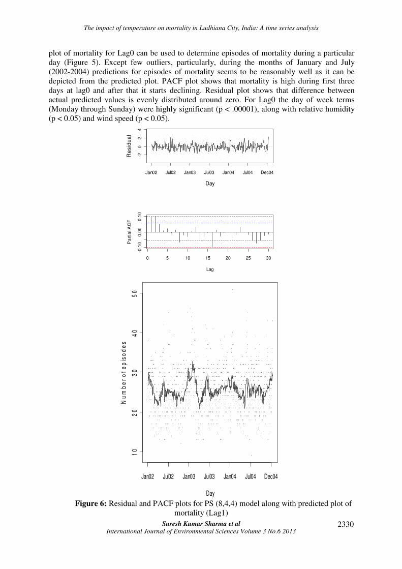
Figure 6: Residual and PACF plots for PS (8,4,4) model along with predicted plot of
mortality (Lag1)
The impact of temperature on mortality in Ludhiana City, India: A time series analysis
Suresh Kumar Sharma et al International Journal of Environmental Sciences Volume 3 No.6 2013
2331
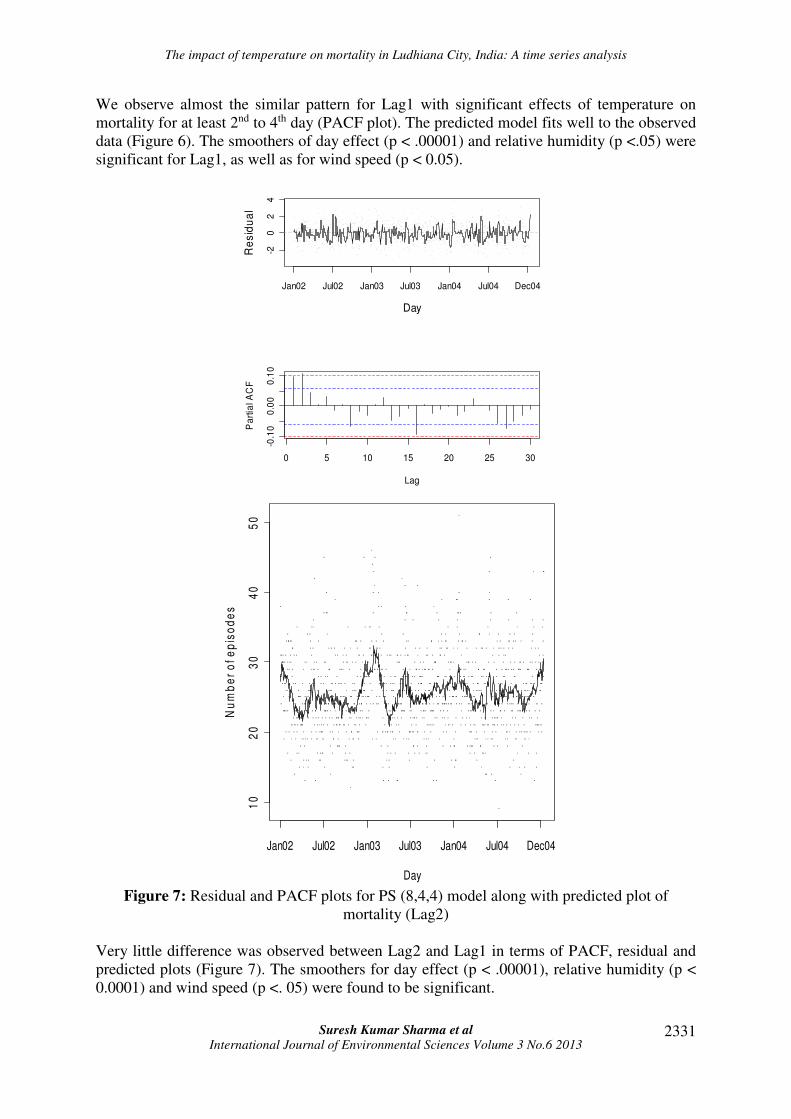
We observe almost the similar pattern for Lag1 with significant effects of temperature on
mortality for at least 2nd to 4th day (PACF plot). The predicted model fits well to the observed
data (Figure 6). The smoothers of day effect (p < .00001) and relative humidity (p <.05) were
significant for Lag1, as well as for wind speed (p < 0.05).
-20
24
Day
Re
sid
ua
l
Jan02 Jul02 Jan03 Jul03 Jan04 Jul04 Dec04
0 5 10 15 20 25 30
-0.1
00
.00
0.1
0
Lag
Pa
rtia
l A
CF
10
20
30
40
50
Day
Nu
mb
er
of
ep
iso
de
s
Jan02 Jul02 Jan03 Jul03 Jan04 Jul04 Dec04
Figure 7: Residual and PACF plots for PS (8,4,4) model along with predicted plot of
mortality (Lag2)
Very little difference was observed between Lag2 and Lag1 in terms of PACF, residual and
predicted plots (Figure 7). The smoothers for day effect (p < .00001), relative humidity (p <
0.0001) and wind speed (p <. 05) were found to be significant.

The impact of temperature on mortality in Ludhiana City, India: A time series analysis
Suresh Kumar Sharma et al International Journal of Environmental Sciences Volume 3 No.6 2013
2332
-4-2
02
4
Day
Re
sid
ua
l
Jan02 Jul02 Jan03 Jul03 Jan04 Jul04 Dec04
0 5 10 15 20 25 30
-0.1
00
.00
0.1
0
Lag
Pa
rtia
l A
CF
10
20
30
40
50
Day
Nu
mb
er
of e
pis
od
es
Jan02 Jul02 Jan03 Jul03 Jan04 Jul04 Dec04
Figure 8: Residual and PACF plots for PS (8,4,4) model along with predicted plot of
mortality (Lag3)
For Lag 3, concentrated band was observed between 20-32 (number of episodes of mortality,
Figure 8) and smoothers for day effect (p < .00001), relative humidity (p < 0.0001) were
significant but non-significant for wind speed (p > 0.05). Temperature and mortality plot
(Figure 9) shows that there are more deaths during summer (> 30 0C) season as compared to
the winter (< 15 0C) season (all cause mortality). It is also evident that from Figure 10 that,
there are more male deaths as compared to female deaths.
3.3 Sensitivity analysis
Separate analysis was carried out for elderly people (age>65 years), however, smaller number
of deaths in 0-4 year’s age group did not allow us to do age specific analysis for this group.
There are more deaths for elder people (> 65 year) during winter season, particularly, when
the temperature is below 15 0C (Figure 11) as compared to summer season. All the Lag
effects except Lag3 were found to be significant (Table 4). For Lag0, Lag1, Lag2 smoothers

The impact of temperature on mortality in Ludhiana City, India: A time series analysis
Suresh Kumar Sharma et al International Journal of Environmental Sciences Volume 3 No.6 2013
2333
were found to be significant for day effect (p < .00001), humidity and wind speed (p < .05).
However, for Lag3, significant smoothers were observed for day effect (p <. 00001) as well
as for relative humidity (p < .01) but non-significant for wind speed (p > .05).
0 200 400 600 800 1000
010
20
30
40
50
Days
Num
ber of D
eath
s
Total DeathsMale DeathsFemale Deaths
Figure 9 and 10: Temperature and Mortality Loess Plot and Daily Number of Deaths (2002-
04)
Figure 11: Temperature and Mortality Plot (>=65 years)

The impact of temperature on mortality in Ludhiana City, India: A time series analysis
Suresh Kumar Sharma et al International Journal of Environmental Sciences Volume 3 No.6 2013
2334
Table 4: Sensitivity Analysis for Elderly People (age≥65 Years)
Penalized Spline Model: PS(8,4,4)
Mean temp 95% CI
Lag
Effects N β-Coeff.
Relative
Risk P-value Lower Upper
Lag 0 1096 0.013014 1.13898783 0.0195 ** 1.021329 1.270201
Lag 1 1095 0.015657 1.16949262 0.000661 * 1.069000 1.279432
Lag 2 1094 0.010214 1.10753852 0.0205 * 1.016007 1.207316
Lag 3 1093 0.007907 1.08228008 0.0687 0.994024 1.178372 * (p<.01), ** (p<.05)
Table 5: Sensitivity Analysis (Female)
Penalized Spline Model: PS(8,4,4)
Mean temp 95% CI
Lag
Effects N β-Coeff.
Relative
Risk P-value Lower Upper
Lag 0 1096 0.018712 1.205771969 0.00117* 1.349536 1.077323
Lag 1 1095 0.019845 1.21951105 0.0000304* 1.799326 0.826536
Lag 2 1094 0.010412 1.109733615 0.0213** 1.212415 1.015749
Lag 3 1093 0.013216 1.141290911 0.00316* 1.245719 1.045617
**(p<.01),**(p<.05)
Table 6: Sensitivity Analysis (Male)
Penalized Spline Model: PS(8,4,4)
Mean temp 95% CI
Lag
Effects N β-Coeff.
Relative
Risk P-value Lower Upper
Lag 0 1096 0.012192 1.129663725 0.00474* 1.229192 1.038195
Lag 1 1095 0.00622 1.064175158 0.078 1.140321 0.993114
Lag 2 1094 0.005259 1.053997418 0.12 1.126077 0.986532
Lag 3 1093 0.00032 1.003203119 0.923 1.069985 0.940589 *(p<.01)
In order to identify the gender sensitivity of the model, separate analysis was carried out for
male and female deaths. Lag0, Lag1, Lag2 and Lag3 effects were significant for females but
for male it was only significant for Lag0. For every 10°C increase in temperature, mortality
for elderly people increased by 1.14%, for female by 1.21% and for males by 1.13%. Also for
every 10°C decreased (below 25°C), mortality increased by 0.88% for elderly, 0.83% for
females and 0.89% for males.
4. Results
The estimated number of deaths in Ludhiana city varies from 9000 to 10000 deaths mid-year
population. The total recorded deaths in Ludhiana city from 2002 – 2004 were 28,007 with an
average of 25.4 deaths per day. If the deaths of non-residents were excluded, the total deaths
were 19335 (69.3%). The age and sex distribution of deaths is shown in Table 2. There were

The impact of temperature on mortality in Ludhiana City, India: A time series analysis
Suresh Kumar Sharma et al International Journal of Environmental Sciences Volume 3 No.6 2013
2335
more deaths among males (65%) and in the above 45 years age group (67%). Only 787
(2.8%) of the deaths were due to accidents and they have been excluded from the analysis.
Most of the deaths (71.2%) fall under the category of “symptoms, signs and abnormalities
classified elsewhere” due to improper certification of the cause of death. The mean (s.d.) of
temperature was 25.6(7.9)°C, relative humidity 58.1(19.3)%, and wind speed 6.87(4.88)
km/hour. The annual mean temperature ranged from 8.1°C to 41.5°C for 2002, 6.2°C to
41.5°C for 2003 and from 8.4°C to 40.6°C for 2004; relative humidity from 11.0% to 93.7%
for 2002, 10.3% to 99.7% for 2003 and from 13.7% to 99.7% for 2004 and wind speed varies
from 0.00 to 42.67 for 2002, 0.00 to 35.67 for 2003 from 0.00 to 27.33 for 2004.
We have worked out the PACF and Residual plots for Lag0, Lag1, Lag2 and Lag3 along with
predicted plot of mortality in R using, PS (8,4,4) model which is having the least GCV score.
It is evident from PACF and Residual plots that there is significant effect of temperature on
mortality.All the Lag effects except Lag3 (Table 4) were found to be significant. For Lag0,
Lag1, Lag2, smoothers were found to be significant for day effect (p < .00001), humidity and
wind speed (p < .05). However, for Lag3, significant smoothers were observed for day effect
(p < .00001) as well as for relative humidity (p < .01) but non-significant for wind speed (p >
.05).
The association between temperature and mortality by smoothing the effects of day of the
week, relative humidity and wind speed was found to be statistically significant. For every
10°C increase in temperature, mortality due to natural causes increased by 1.17% and for
every 10°C decrease in temperature (below 25°C), mortality increased by 0.86%. Sensitivity
analysis was carried out separately for deaths in the 65+ year’s age group and gender. Smaller
number of deaths in 0-4 year’s age group did not allow us to do age specific analysis.
Sensitivity analysis shows that elderly (> 65 years) population was much affected by
temperature variations. For every 10°C increase in temperature, mortality for elderly people
increased by 1.14%, for female by 1.21% and for males by 1.13%. Also for every 10°C
decreased (below 25°C), mortality increased by 0.88% for elderly, 0.83% for females and
0.89% for males.
5. Discussion
As a part of the Health Effects Institute, Boston USA, project, this paper gives the impact of
temperature on mortality in Ludhiana City of India. The mortality rates of Urban Punjab for
the years 2002, 2003 and 2004 were 6.2, 6.0 and 7.2 deaths per 1,000 mid-year population
(Source: SRS Bulletin). Apart from the analysis of the relation between temperature and
mortality in the city, the smoothing effects of day, relative humidity and wind speed have
also been worked out. The PACF i.e. partial autocorrelation function and residual plots were
plotted for Lag0, Lag1, Lag2 and Lag3 along with the predicted plots (all cause mortality). It
is evident from PACF and Residual plots that there is significant effect of temperature on
mortality after smoothing the effects of day, relative humidity and wind speed.
Sensitivity analysis was carried out separately for deaths in the 65+ year’s age group as well
for gender. Smaller number of deaths in 0-4 year’s age group did not allow us to do age
specific analysis. Sensitivity analysis shows that elderly (> 65 years) population was much
affected by temperature variations, particularly, during winter season. Studies based on
retrospective data face several difficulties and this study is no exception. On the basis of the
age-specific mortality rates and age distribution of the population of urban India, it seems that
about 15-23% may not have been registered in various age groups, however, there is no

The impact of temperature on mortality in Ludhiana City, India: A time series analysis
Suresh Kumar Sharma et al International Journal of Environmental Sciences Volume 3 No.6 2013
2336
suggestion that this proportion would vary day by day. In conclusion there is need to improve
the overall registration system of deaths. Cause specific analysis was not possible as cause of
death was not clearly mentioned in most of the cases. It seems there is under reporting of
deaths, particularly, among children below the age of 5 years. We suggest that ICD-10 coding
system should be introduced properly so that each case should have proper code and cause-
specific analysis may be performed to get better results in future.
Acknowledgments
We are thankful to Birth and Death Registration Office, Ludhiana; Meteorological
Department, New Delhi and Health Effects Institute, Boston.
6. References
1. Anderson B.G., and Bell M.L., (2009), Weather-related mortality: how heat, cold, and
heat waves affect mortality in the United States. Epidemiology, 20(2), pp 205-213.
2. Baker DANM, (2008), Environmental Epidemiology: Study Methods and Application,
Oxford University Press.
3. Ballester F., Corella D., Perez-Hoyos S., Saez M.and Hervas A.,(1997), Mortality as a
function of temperature. A study in Valencia, Spain, 1991 1993, International Journal
ofJ Epidemiology, 26(3),pp 551-561.
4. Ballester J., Robine J.M., Herrmann F.R. and Rodo X, (2011), Long-term projections
and acclimatization scenarios of temperature-related mortality in Europe, Nat
Communications , 2, pp 358.
5. Barron D.N., (1992), The Analysis of Count Data: Overdispersion and
Autocorrelation, Social Methodology, 22, pp 179-220.
6. Basu, R.,(2009), High ambient temperature and mortality: A review of epidemiologic
studies from 2001 to 2008. Environmental Health, doi:10.1186/1476-069X-8-40.
7. Basu R. and Malig B, (2011), High ambient temperature and mortality in California:
Exploringthe roles of age, disease, and mortality displacement. Environmental
Research, 111(8), pp 1286-1292.
8. Braga A.L., Zanobetti A. and Schwartz J. (2001), The time course of weather related
deaths, Epidemiology, 12, pp 662–667.
9. Carson C., Hajat S., Armstrong B.,and Wilkinson P, 2006, Declining vulnerability to
temperature related mortality in London over the 20th century, American Journal of
Epidemiology, 164(1), pp 77-84.
10. Curriero F.C., Heiner K.S., Samet J.M., Zeger S.L., Strug L. and Patz J.A.,2002,
Temperature and mortality in 11 cities of the eastern United States, American Journal
of Epidemiology, 155(1), pp 80-87.
11. Ellis F.P., and Nelson F.,(1978), Mortality in the elderly in a heat wave in New York
City, Environmental Research, 15, pp 504-512.
The impact of temperature on mortality in Ludhiana City, India: A time series analysis
Suresh Kumar Sharma et al International Journal of Environmental Sciences Volume 3 No.6 2013
2337
12. Fouillet A., Rey G. And Laurent F, (2006), Excess mortality related to the August
2003 heat wave in France, International Archives of Occupational and Environmental
Health, 80,pp 16-24.
13. Goldberg M.S., Gasparrini A., Armstrong B. and Valois M.F., (2011), The short-term
influence of temperature on daily mortality in the temperate climate of Montreal,
Canada. Environmental Research, 111(6), pp 853-860.
14. Hajat, S., Armstrong B., Baccini M., Biggeri A., Bisanti L., Russo A., Paldy A.,
Menne B.and Kosatsky T., 2006, Impact of high temperatures on mortality: is there an
added “heat wave” effect? Epidemiology, 17, pp 632-638.
15. Hajat S., Kovats R.S., Atkinson R.W. and Haines A.,(2002), Impact of hot
temperatures on death in London: a time series approach. J Epidemiol Community
Health, 56(5), pp 367-372.
16. Ha J., Shin Y. and Kim H.,(2011), Distributed lag effects in the relationship between
temperature and mortality in three major cities in South Korea, Science of the Total
Environment ,409(18), pp 3274-3280.
17. Hoffmann B., Hertel S., Boes T., Weiland D. and Jockel K.H.:, (2008), Increased
cause-specific mortality associated with 2003 heat wave in Essen, Germany, Journal
of Toxicology and Environmental Health, 71(11-12), pp 759-765.
18. Huynen, M.M., Martens, P., Schram, D.,Weijenberg, M.P. and Kunst, A.E.,(2001),
The impact of heat waves and cold spells on mortality rates in the Dutch population.
Environmental Health Perspectives, 109, pp 463-470.
19. Kim H., Ha J.S. and Park J. ,(2006), High temperature, heat index, and mortality in 6
major cities in South Korea, International Archives of Occupational and
Environmental Health, 61(6), pp 265-270.
20. Kumar R., Sharma S., Thakur J.S., Lakshmi P.V.M., Sharma M.K. and Singh T.,
(2010), Association of air pollution and mortality in the Ludhiana City of India: A
time Series Study, Indian Journal of Public Health , 54( 2) , pp 98-103.
21. McKee C.M.,(1989), Deaths in winter: can Britain learn from Europe? European
Journal of Epidemiology, 5(2), pp178-182.
22. Muggeo V.M., (2008), Modeling temperature effects on mortality: multiple
segmentedrelationships with common break points, Biostatistics, 9(4), pp 613-620.
23. Ostro B.D., Roth L.A., Green R.S. and Basu R, (2009), Estimating the mortality effect
of the July 2006 California heat wave, Environmental Research , 109(5), pp 614-619.
24. Peng R.D., Dominici F. and Louis T.A., (2006), Model Choice in Time Series Studies
of Air Pollution and Mortality, Journal of the Royal Statistical Society Part A, 169(2),
pp 179-203.
25. Schwartz J., (2000), The distributed lag between air pollution and daily deaths,
Epidemiology, 11(3), pp 320- 326.

The impact of temperature on mortality in Ludhiana City, India: A time series analysis
Suresh Kumar Sharma et al International Journal of Environmental Sciences Volume 3 No.6 2013
2338
26. Yu W., Guo Y., Ye X., Wang X., Huang C., Pan X. and Tong S., (2011),The effect of
various temperature indicators on different mortality categories in a subtropical city of
Brisbane, Australia, Science of the Total Environment , 409(18), pp 3431-3437.
27. Hastie T.J. and Tibshirani R.J., (1990), Generalized Additive Models,Chapman and
Hall/CRC, London.
28. Peng R.D. and Dominici F., (2008), Statistical methods for environmental
epidemiology in R, Springer, NewYork .
29. Wood S.N.,(2006), Generalized Additive Model: an introduction with R, Chapman
and Hall/CRC, New York.