Embed Size (px)
Citation preview
The Impact of Transit-Oriented Development on Residential Property Value
in King County, WA
Simin Xu
A thesis
submitted in partial fulfillment of the
requirements for the degree of
Master of Urban Planning
University of Washington
2015
Committee:
Qing Shen
Christopher Bitter
Program Authorized to Offer Degree:
College of Built Environments

©Copyright 2015
Simin Xu
I
University of Washington
Abstract
The Impact of Transit-Oriented Development on Residential Property Value in King County, WA
Simin Xu
Chair of the Supervisory Committee:
Professor Qing Shen
Department of Urban Design and Planning
Transit-Oriented Development (TOD) has long been a powerful tool for improving sustainable urban
development. A well-designed TOD project enhances the accessibility to different kinds of activities,
decreases transportation cost, and increases the travel comfortable level, thereby expanding the
willingness to pay for the properties around it. This study measures the impact of Transit-Oriented
Development on single-family property value within 1.5 mile radius around Renton Transit Center, a
TOD project implemented 18 years ago in King County, WA. Using time-series Hedonic Price Analysis
(HPA), results of this study corroborate the mainstream view that TOD has premium effects on
surrounding property values. Controlling other variables affecting housing price, increasing the
accessibility to the Transit Center by one standard deviation distance (1890 feet, or about 0.36 mile) is
associated with an 11% increase of the housing price during TOD-construction time. In post-TOD time,
increasing the accessibility by one standard deviation distance (1781 feet, or about 0.33 mile) is linked
to a 13% increase of the housing price. Results for time-series dummy variables show that properties
sold at a lower price in pre-TOD time than those after TOD took into effect. Then, Hedonic Method is
used for three time intervals of before-TOD, during-TOD, and post-TOD. Results show that the
insignificant influence of TOD accessibility before TOD operation becomes significantly positive after
TOD took place. However, the premium effect of TOD could be reduced due to TOD-related nuisance.
Properties located in areas with high percentage of commercial uses and very compact street network
systems were sold at a discount. This suggests that besides benefiting from station accessibility, station
area properties may also have suffered from TOD-related nuisance that can reduce the benefits to some
extent. Findings suggest that local government under fiscal stress could generate additional revenue

II
source through innovative TOD projects and programs, yet to find an appropriate strategy for mixed
land use development near the station also needs to be considered.
III
TABLE OF CONTENTS
Table of contents ....................................................................................................................................... III
List of tables ................................................................................................................................................V
List of figures ............................................................................................................................................ VI
Chapter 1 Introduction ................................................................................................................................ 1
1.1 Background .................................................................................................................................. 1
1.2 Purpose and structure ................................................................................................................... 3
Chapter 2 Literature review ........................................................................................................................ 4
2.1 Property value capitalization from TOD ........................................................................................... 4
2.2 Other factors affecting residential property value .......................................................................... 13
2.1.1 Social and economic related factors ........................................................................................ 13
2.2.2 Other locational related factors ................................................................................................ 16
2.3 Summary of literature review ......................................................................................................... 18
Chapter 3 Study area ................................................................................................................................ 21
3.1 Study area selection criteria ............................................................................................................ 21
3.2 Study area description ..................................................................................................................... 21
Chapter 4 Data and methodology ............................................................................................................. 25
4.1 Methodology ................................................................................................................................... 25
4.1.1 Two time-series models ........................................................................................................... 26
4.1.2 Before-during-after models ...................................................................................................... 27
4.2 Data ................................................................................................................................................. 28
4.2.1 Data types ................................................................................................................................. 28
4.2.2 Data filtering ............................................................................................................................ 30
4.2.3 Data by category ...................................................................................................................... 33
IV
4.3 Descriptive statistics of the data ..................................................................................................... 39
Chapter 5 Model results ............................................................................................................................ 43
5.1 Results of time-series models ......................................................................................................... 43
5.2 Results of before-during-after models ............................................................................................ 50
Chapter 6 Conclusion ................................................................................................................................ 58
References ............................................................................................................................................... 61
Appendix ................................................................................................................................................... 65
V
LIST OF TABLES
Table 1 - Summary of studies on impact of TOD proximity on property value – 1) ................................. 7
Table 2 - Summary of studies on impact of TOD proximity on property value – 2) ................................. 8
Table 3- Summary of studies on impact of TOD proximity on property value – 3) .................................. 9
Table 4 - Time-series observations ........................................................................................................... 26
Table 5 - Data description and data source ............................................................................................... 37
Table 6 - Descriptive statistics of time-series models .............................................................................. 39
Table 7 - Descriptive statistics of before-after models ............................................................................. 41
Table 8 - Regression results for Model 1 & Model 2 ............................................................................... 43
Table 9 - Regression results for Model 3, 4 and 5 .................................................................................... 50
Table 10 - Regression results for Model 6, 7 and 8 .................................................................................. 52
Table 11 - z-test results ............................................................................................................................. 57
VI
LIST OF FIGURES
Figure 1 - Positive and negative influences on residential land prices of proximity to non-residential land
uses (source: Li and Brown, 1980) ............................................................................................................. 6
Figure 2 - Conceptual model of factors affecting residential property value ........................................... 19
Figure 3 - Transit-oriented development process in Renton Transit Center; ©2015 Google Imagery .... 22
Figure 4 - Home price index in Seattle (Source: S&P/ Case & Shiller Home Price Indices) .................. 29
Figure 5 - 1.5 mile buffer of Renton Transit Center ................................................................................. 32
Figure 6 - Unstandardized coefficients of distance dummy variables ...................................................... 47
Figure 7 - Unstandardized coefficients of time-series dummy variables ................................................. 49
Figure 8 - Unstandardized coefficients of distance dummy variables for three time intervals ................ 55
Figure 9 - Variation in inflated housing price at four distance ranges to TOD ........................................ 56
1
CHAPTER 1 INTRODUCTION
1.1 BACKGROUND
The U.S. has faced enormous sustainable challenges since the last century. Perhaps the most obvious
challenge was turning from mass transit to a car-dependent society. Beginning after World War II, total
annual passenger trips of public transportation in U.S fell by 69%, from 22.3 billion in 1945 to only 8.0
billion in 1975 (John Pucher, 2004). Together with substantially decline of public transportation
ridership, is the rapidly increase of private car ownership, energy consumption, and environmental
pollution. State and local government began to see this, realized that they could do something to
improve public transportation. In the approximately 30 years after 1975, state and local expenditures in
public transportation rose from $3.2 billion to $22.8 billion, the total annual passenger trips only rose
from 8.0 billion in 1975 to 9.5 billion in 2001 (John Pucher, 2004). This trend of rising state and local
investment in public transportation has continued in the last decades, but public transportation in U.S
still facing challenges.
Solving transportation problem is not simple, and not only lie in improving public transportation.
Perhaps the most fundamental underlying source for concomitant decline in mass transit service is the
dispersed low-density suburban development –urban sprawl. Therefore, encouraging transit-oriented
development (TOD) - a compact, mixed-use development near transit facilities with high-quality
walking environment is a new approach to solve the long-term sustainable challenge. The State of
California was the pioneer in implementing large TODs. From 1990 to 2000, California invested
approximately 14 billion dollars of state funds on mass transportation programs, in result, 21 TOD
projects have been implemented over 15 years (California Department of Transportation, 2002). From
2004 to 2014, the Federal Transit Administration (FTA) allocated $18.9 billion to build new or
expanded transit systems which involve an important goal of promoting TOD through the Capital
Investment Grant program (United States Government Accountability Office, 2014).
Transit-Oriented Development is a solution to improve transportation system, reduce carbon footprint,
and improve equity by providing more residents with good opportunity to housing, jobs and services
(Cervero et al., 2004). The benefit of being accessible to various kind of services can get capitalized into

2
market value of land and property. Therefore, TOD could be development-based incentive to capitalize
land value by selling or leasing land to explore development opportunities around transit station areas.
The increases of land value due to public investment in infrastructure and changes in land use
regulations could generate more revenue source which could be used to further finance TOD projects
without significant fiscal distortion (World Bank Group, 2015). The increasing land value may attract
more commercial and service activities in the station areas, thus further increase land value, promote
employment, and shaping the city’s vibrancy.
Planning is a process involving values of different stakeholders, planning for Transit-Oriented
Development is also the case. Stakeholders who work to promote the monetary value of land, including
bankers, lawyers, real estates, developers, and local government, are interested in future profits
generated by TOD. On the one hand, it is essential for almost all financial decision making. On the other
hand, since TOD generally entails higher construction costs and accompanying risks, which could
inhibit stakeholders pursuing these projects, therefore knowing how much future profit that can generate
by TOD to offset the investment costs is very important. Moreover, since diverse groups’ interests are
often interdependent in planning process, particular stakeholders’ interest in promoting land values are
corresponding with environmentalists encouraging less carbon emission, sharing with commuters
promoting better public transit services, and community residents seeking better outcome of equity.
Thus, this thesis may also improve the overall outcome, satisfying people with other perspectives by in
particular addressing some stakeholders’ interests.
This thesis is to give an empirical case study about the extent, both in time and space, a completed TOD
project fulfilled the promise of residential property value capitalization in Seattle Metropolitan Area, and
which TOD components (transit accessibility, mixed land use, and walkable pedestrian design) are more
beneficial to land price than others, in order to guide better investment decision making.
3
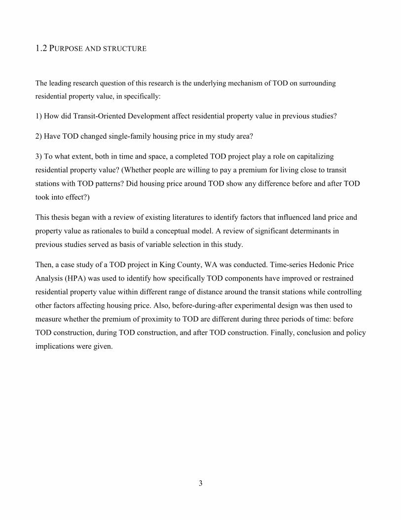
1.2 PURPOSE AND STRUCTURE
The leading research question of this research is the underlying mechanism of TOD on surrounding
residential property value, in specifically:
1) How did Transit-Oriented Development affect residential property value in previous studies?
2) Have TOD changed single-family housing price in my study area?
3) To what extent, both in time and space, a completed TOD project play a role on capitalizing
residential property value? (Whether people are willing to pay a premium for living close to transit
stations with TOD patterns? Did housing price around TOD show any difference before and after TOD
took into effect?)
This thesis began with a review of existing literatures to identify factors that influenced land price and
property value as rationales to build a conceptual model. A review of significant determinants in
previous studies served as basis of variable selection in this study.
Then, a case study of a TOD project in King County, WA was conducted. Time-series Hedonic Price
Analysis (HPA) was used to identify how specifically TOD components have improved or restrained
residential property value within different range of distance around the transit stations while controlling
other factors affecting housing price. Also, before-during-after experimental design was then used to
measure whether the premium of proximity to TOD are different during three periods of time: before
TOD construction, during TOD construction, and after TOD construction. Finally, conclusion and policy
implications were given.
4
CHAPTER 2 LITERATURE REVIEW
2.1 PROPERTY VALUE CAPITALIZATION FROM TOD
While there is no universally accepted definition of TOD, it is generally composed of many common
parts, including transit accessibility, mixed use of land near transit station and pedestrian oriented design
(Metropolitan Atlanta Rapid Transit Authority, Maryland Transit Administration, Bay Area Rapid
Transit Authority, Washington Metropolitan Area Transit Authority, and King County Metro). These
components working together and in result enhance the accessibility to different kinds of activities,
decrease transportation cost, and also increase the travel comfortable level, thereby expand the
willingness to pay for the properties located around it.
Classic economics theories proposed that the maximum amount a land user can pay for the land in a
particular location is determined by amenities of the land. Back to 1826, Von Thunen (1826)’s Model
illustrates that transportation saving is the determinant of land rent, explains why land prices are higher
in some locations than in others. Alonso (1964) also proposed that the development of transportation
infrastructure and the resulting drop in transportation costs and increase in accessibility levels are
closely related to changes in housing values. These statements justify that why being near TOD would
enhance the surrounding housing price.
The premiums of TOD on property value around station area could be disintegrated into several parts:
• First, the introduction of transit service into the neighborhood increases travel options for
residents and employees of the area and can reduce travel time to the CBD and other activity
centers (Fejarang, 1994). It is the increase of transportation accessibility that transfers into land
values.
• Second, one of important TOD characteristic – high degree of mixed land use near station area
largely enhances local convenience to different kinds of non-residential daily activities, such as
shopping, schools, park and recreation within walking distance. The increasing in proximity and
convenience to other non-residential activities has been linked to shorter daily travel distances,
lower vehicle trip rates, and fewer total vehicle miles of travel (Ewing and Cervero, 2010). It is
this mixed-use advantage that being capitalized into land values.
5
• Third, another component of transit-oriented development for most project is pedestrian friendly
design, which could also affect housing prices. Typically, interconnected streets and smaller
blocks are more likely to attract home buyers to pay a premium for their houses than large blocks
and cul-de-sacs street design (Bartholomew and Ewing, 2011).
• Fourth, better transit services, proximity to non-residential activities and pedestrian friendly
design would attract more population, as well as new investments and businesses thereby
creating new employment around station area. The revitalizing economics will spur land values.
This effect is largely redistributive, since the relative gains around transit stations are matched by
relative losses for properties and businesses that lie away from stations (Robert Cervero, 2004).
Moreover, sometimes there is double-counting influence of these multiplicity of benefits (Robert,
Cervero, 2004). Therefore, one cannot look at these effects separately, because they are coordinate and
mutually reinforcing, and the overall premium of TOD is always larger than simply adding the value
from each components.
However, we must have a clear picture of the dual nature of these influences. Being too close to transit
station sometimes will not enhance, but negatively affects housing price. Same thing is that being too
proximity to the center of non-residential activities would also decrease property value around it though
the convenience to reach commercial activities provided by mixed land uses are favorable to housing
market. These phenomena show that property value influenced by TOD vary considerably by settings,
and also by how different home buyers trade-off between the advantages and disadvantage of different
components of TOD, and between the benefits of overall TOD effects and the influences from other
variables such as social-economic condition changes. For example, a trade-off that people frequently
make is between the nuisance of station area parking lot and the accessibility to station. People dislike
being too close to parking lot around transit stations. A study has suggested that the prices of homes in
park and ride station areas suffer a 1.9 percent price decrease for over 10-year period (Kahn, 2007).
Same thing is for nonresidential land uses. An early study from Grether and Mieszkowski (1980)
analyzed the impacts of nonresidential land uses on prices of housing in New Haven, Connecticut,
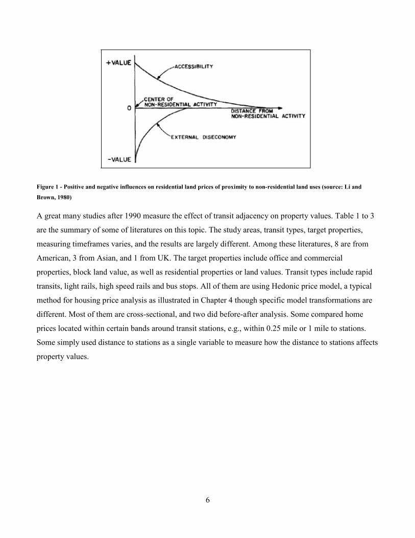
indicating that proximity to nonresidential area actually have negative price effect. Li and Brown (1980)
found that the impacts of the negative externalities decrease more rapidly with distance than the positive
effects of accessibility. As a result, land price and property value will adjust to achieve a locational
equilibrium. This is why sometimes properties located at least some distance away from TOD have
significantly higher values than those in the station area.
6
Figure 1 - Positive and negative influences on residential land prices of proximity to non-residential land uses (source: Li and
Brown, 1980)
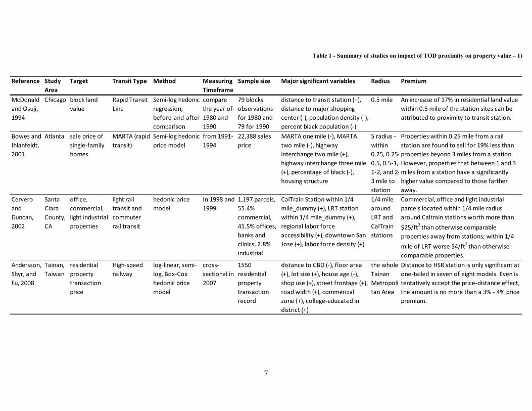
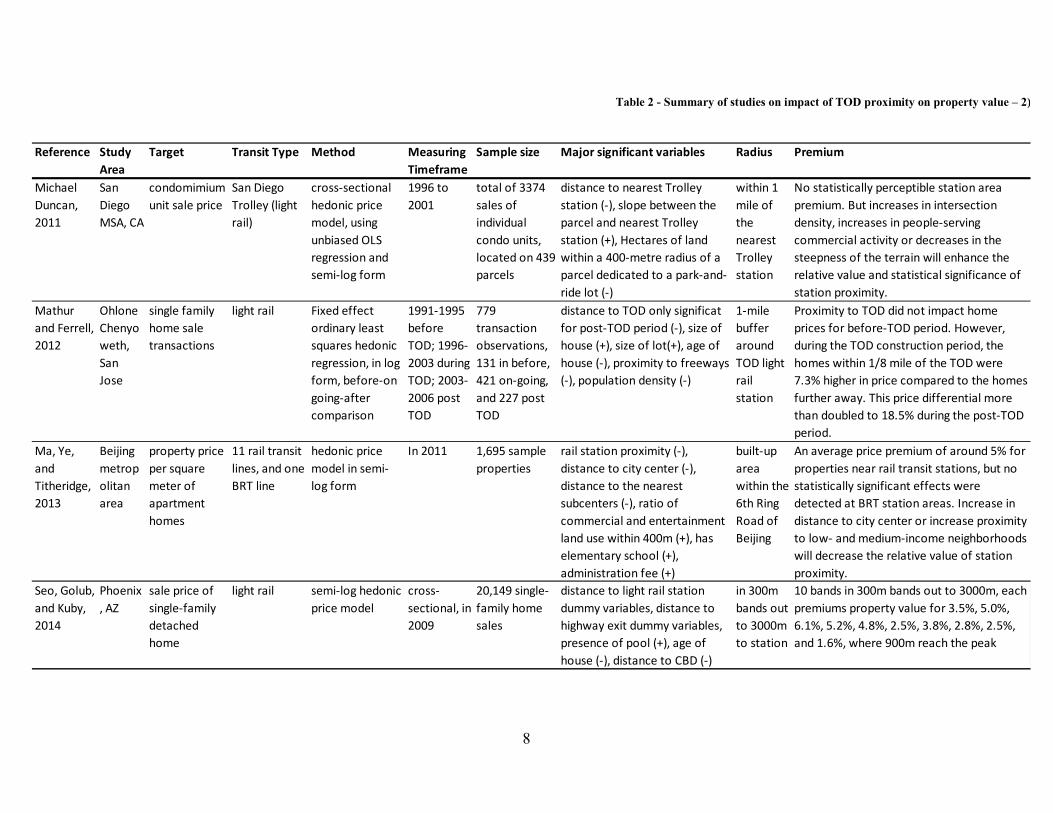
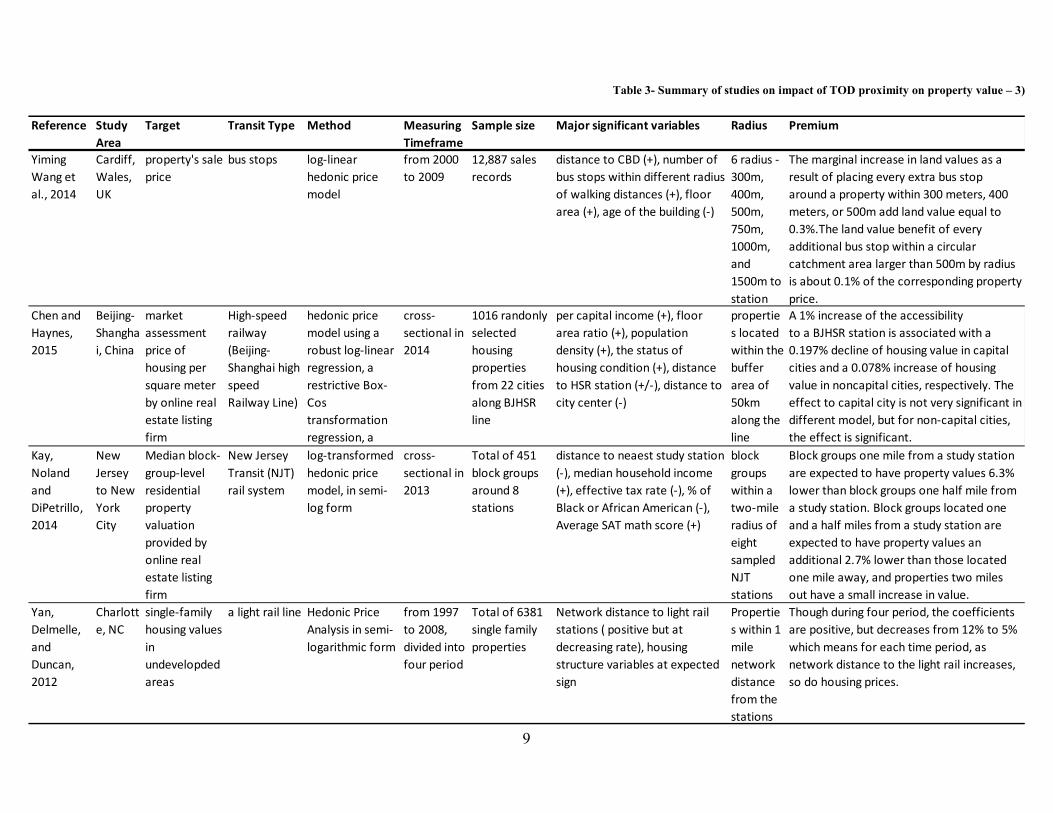
A great many studies after 1990 measure the effect of transit adjacency on property values. Table 1 to 3
are the summary of some of literatures on this topic. The study areas, transit types, target properties,
measuring timeframes varies, and the results are largely different. Among these literatures, 8 are from
American, 3 from Asian, and 1 from UK. The target properties include office and commercial
properties, block land value, as well as residential properties or land values. Transit types include rapid
transits, light rails, high speed rails and bus stops. All of them are using Hedonic price model, a typical
method for housing price analysis as illustrated in Chapter 4 though specific model transformations are
different. Most of them are cross-sectional, and two did before-after analysis. Some compared home
prices located within certain bands around transit stations, e.g., within 0.25 mile or 1 mile to stations.
Some simply used distance to stations as a single variable to measure how the distance to stations affects
property values.
7
Reference Study
Area
Target Transit Type Method Measuring
Timeframe
Sample size Major significant variables Radius Premium
McDonald
and Osuji,
1994
Chicago block land
value
Rapid Transit
Line
Semi-log hedonic
regression,
before-and-after
comparison
compare
the year of
1980 and
1990
79 blocks
observations
for 1980 and
79 for 1990
distance to transit station (+),
distance to major shopping
center (-), population density (-),
percent black population (-)
0.5 mile An increase of 17% in residential land value
within 0.5 mile of the station sites can be
attributed to proximity to transit station.
Bowes and
Ihlanfeldt,
2001
Atlanta sale price of
single-family
homes
MARTA (rapid
transit)
Semi-log hedonic
price model
from 1991-
1994
22,388 sales
price
MARTA one mile (-), MARTA
two mile (-), highway
interchange two mile (+),
highway interchange three mile
(+), percentage of black (-),
housing structure
5 radius -
within
0.25, 0.25-
0.5, 0.5-1,
1-2, and 2-
3 mile to
station
Properties within 0.25 mile from a rail
station are found to sell for 19% less than
properties beyond 3 miles from a station.
However, properties that between 1 and 3
miles from a station have a significantly
higher value compared to those farther
away.
Cervero
and
Duncan,
2002
Santa
Clara
County,
CA
office,
commercial,
light industrial
properties
light rail
transit and
commuter
rail transit
hedonic price
model
In 1998 and
1999
1,197 parcels,
55.4%
commercial,
41.5% offices,
banks and
clinics, 2.8%
industrial
CalTrain Station within 1/4
mile_dummy (+), LRT station
within 1/4 mile_dummy (+),
regional labor force
accessibility (+), downtown San
Jose (+), labor force density (+)
1/4 mile
around
LRT and
CalTrain
stations
Commercial, office and light industrial
parcels located within 1/4 mile radius
around Caltrain stations worth more than
$25/ft2
than otherwise comparable
properties away from stations; within 1/4
mile of LRT worse $4/ft2
than otherwise
comparable properties.
Andersson,
Shyr, and
Fu, 2008
Tainan,
Taiwan
residential
property
transaction
price
High-speed
railway
log-linear, semi-
log, Box-Cox
hedonic price
model
cross-
sectional in
2007
1550
residential
property
transaction
record
distance to CBD (-), floor area
(+), lot size (+), house age (-),
shop use (+), street frontage (+),
road width (+), commercial
zone (+), college-educated in
district (+)
the whole
Tainan
Metropoli
tan Area
Distance to HSR station is only significant at
one-tailed in seven of eight models. Even is
tentatively accept the price-distance effect,
the amount is no more than a 3% - 4% price
premium.
Table 1 - Summary of studies on impact of TOD proximity on property value – 1)
8
Reference Study
Area
Target Transit Type Method Measuring
Timeframe
Sample size Major significant variables Radius Premium
Michael
Duncan,
2011
San
Diego
MSA, CA
condomimium
unit sale price
San Diego
Trolley (light
rail)
cross-sectional
hedonic price
model, using
unbiased OLS
regression and
semi-log form
1996 to
2001
total of 3374
sales of
individual
condo units,
located on 439
parcels
distance to nearest Trolley
station (-), slope between the
parcel and nearest Trolley
station (+), Hectares of land
within a 400-metre radius of a
parcel dedicated to a park-and-
ride lot (-)
within 1
mile of
the
nearest
Trolley
station
No statistically perceptible station area
premium. But increases in intersection
density, increases in people-serving
commercial activity or decreases in the
steepness of the terrain will enhance the
relative value and statistical significance of
station proximity.
Mathur
and Ferrell,
2012
Ohlone
Chenyo
weth,
San
Jose
single family
home sale
transactions
light rail Fixed effect
ordinary least
squares hedonic
regression, in log
form, before-on
going-after
comparison
1991-1995
before
TOD; 1996-
2003 during
TOD; 2003-
2006 post
TOD
779
transaction
observations,
131 in before,
421 on-going,
and 227 post
TOD
distance to TOD only significat
for post-TOD period (-), size of
house (+), size of lot(+), age of
house (-), proximity to freeways
(-), population density (-)
1-mile
buffer
around
TOD light
rail
station
Proximity to TOD did not impact home
prices for before-TOD period. However,
during the TOD construction period, the
homes within 1/8 mile of the TOD were
7.3% higher in price compared to the homes
further away. This price differential more
than doubled to 18.5% during the post-TOD
period.
Ma, Ye,
and
Titheridge,
2013
Beijing
metrop
olitan
area
property price
per square
meter of
apartment
homes
11 rail transit
lines, and one
BRT line
hedonic price
model in semi-
log form
In 2011 1,695 sample
properties
rail station proximity (-),
distance to city center (-),
distance to the nearest
subcenters (-), ratio of
commercial and entertainment
land use within 400m (+), has
elementary school (+),
administration fee (+)
built-up
area
within the
6th Ring
Road of
Beijing
An average price premium of around 5% for
properties near rail transit stations, but no
statistically significant effects were
detected at BRT station areas. Increase in
distance to city center or increase proximity
to low- and medium-income neighborhoods
will decrease the relative value of station
proximity.
Seo, Golub,
and Kuby,
2014
Phoenix
, AZ
sale price of
single-family
detached
home
light rail semi-log hedonic
price model
cross-
sectional, in
2009
20,149 single-
family home
sales
distance to light rail station
dummy variables, distance to
highway exit dummy variables,
presence of pool (+), age of
house (-), distance to CBD (-)
in 300m
bands out
to 3000m
to station
10 bands in 300m bands out to 3000m, each
premiums property value for 3.5%, 5.0%,
6.1%, 5.2%, 4.8%, 2.5%, 3.8%, 2.8%, 2.5%,
and 1.6%, where 900m reach the peak
Table 2 - Summary of studies on impact of TOD proximity on property value – 2)
9
Reference Study
Area
Target Transit Type Method Measuring
Timeframe
Sample size Major significant variables Radius Premium
Yiming
Wang et
al., 2014
Cardiff,
Wales,
UK
property's sale
price
bus stops log-linear
hedonic price
model
from 2000
to 2009
12,887 sales
records
distance to CBD (+), number of
bus stops within different radius
of walking distances (+), floor
area (+), age of the building (-)
6 radius -
300m,
400m,
500m,
750m,
1000m,
and
1500m to
station
The marginal increase in land values as a
result of placing every extra bus stop
around a property within 300 meters, 400
meters, or 500m add land value equal to
0.3%.The land value benefit of every
additional bus stop within a circular
catchment area larger than 500m by radius
is about 0.1% of the corresponding property
price.
Chen and
Haynes,
2015
Beijing-
Shangha
i, China
market
assessment
price of
housing per
square meter
by online real
estate listing
firm
High-speed
railway
(Beijing-
Shanghai high
speed
Railway Line)
hedonic price
model using a
robust log-linear
regression, a
restrictive Box-
Cos
transformation
regression, a
cross-
sectional in
2014
1016 randonly
selected
housing
properties
from 22 cities
along BJHSR
line
per capital income (+), floor
area ratio (+), population
density (+), the status of
housing condition (+), distance
to HSR station (+/-), distance to
city center (-)
propertie
s located
within the
buffer
area of
50km
along the
line
A 1% increase of the accessibility
to a BJHSR station is associated with a
0.197% decline of housing value in capital
cities and a 0.078% increase of housing
value in noncapital cities, respectively. The
effect to capital city is not very significant in
different model, but for non-capital cities,
the effect is significant.
Kay,
Noland
and
DiPetrillo,
2014
New
Jersey
to New
York
City
Median block-
group-level
residential
property
valuation
provided by
online real
estate listing
firm
New Jersey
Transit (NJT)
rail system
log-transformed
hedonic price
model, in semi-
log form
cross-
sectional in
2013
Total of 451
block groups
around 8
stations
distance to neaest study station
(-), median household income
(+), effective tax rate (-), % of
Black or African American (-),
Average SAT math score (+)
block
groups
within a
two-mile
radius of
eight
sampled
NJT
stations
Block groups one mile from a study station
are expected to have property values 6.3%
lower than block groups one half mile from
a study station. Block groups located one
and a half miles from a study station are
expected to have property values an
additional 2.7% lower than those located
one mile away, and properties two miles
out have a small increase in value.
Yan,
Delmelle,
and
Duncan,
2012
Charlott
e, NC
single-family
housing values
in
undevelopded
areas
a light rail line Hedonic Price
Analysis in semi-
logarithmic form
from 1997
to 2008,
divided into
four period
Total of 6381
single family
properties
Network distance to light rail
stations ( positive but at
decreasing rate), housing
structure variables at expected
sign
Propertie
s within 1
mile
network
distance
from the
stations
Though during four period, the coefficients
are positive, but decreases from 12% to 5%
which means for each time period, as
network distance to the light rail increases,
so do housing prices.
Table 3- Summary of studies on impact of TOD proximity on property value – 3)
10
Among these literatures, most found that proximity to transit stations leads to property value increase
(McDonald and Osuji, 1994; Cervero and Duncan, 2002; Mathur and Ferrell, 2012; Ma, Ye, and
Titheridge, 2013; Yiming Wang et. Al., 2014; Seo, Golub, and Kuby, 2014; Kay, Noland and DiPetrillo,
2014). Though similar results are found in different studies, the relative impacts of accessibility to
station are also different. Also, since different studies used different forms of regression methods, some
interpreted the premium as percentage change of price as a unit increase of distance to station, some
interpreted as price elasticity. In addition, some measured distance by series of dummy variables, but the
reference groups varies. These reasons make the results of premium difficult to compare. Generally,
using otherwise comparable housing outside station area (inconsistent in different studies) as control
group, the premium effects of station proximity (on properties located 1/8 to ½ mile distance to station)
vary from 3.5% to 25% as these studies show. Cervero (2004) ’s meta-analysis showed that price
premiums for housing located within a ¼ to ½ mile radius of rail transit station of between 6.4 % and
45 % comparing to equivalent housing outside of the station areas.
However, the statement that proximity to stations has premium effects on property values were not
corroborated by the evidence from other studies. Three studies found that there is no statistically
perceptible station area premium near station area, one for high-speed-rail in Taiwan, one for light rail in
U.S., and one for bus rapid transit in Beijing (Andersson, Shyr, and Fu, 2008; Michael Duncan, 2011;
Ma, Ye, and Titheridge, 2013). Some even indicated a negative relationship (Bowes and Ihlanfeldt,
2001; Yan, Delmelle, and Duncan, 2012; Chen and Haynes, 2015). However, among these literatures,
some found proximity to stations will increase property value only if conditional upon other variables
such as intersection density, commercial activity, intersection density, distance to city center, and
income level of neighborhoods (Michael Duncan, 2011; Ma, Ye, and Titheridge, 2013). Some suggested
that though the negative relationship exists between proximity to station and housing price, the
coefficients became smaller during TOD operation time comparing with before-TOD time (Yan,
Delmelle, and Duncan, 2012). These mean station proximity still plays a role in increasing property
value if not considering other effects.
Previous studies have yielded vastly different results ranging from proximity to station significantly
increases property values, to negatively affect property values or have no significant relationship with
property value. These different results of previous studies are because of several reasons:
11
• First, impacts of station proximity are conditional upon changes of other variables. Though
distance to station matters, as most studies concluded, the relationship is not as simple as a linear
function. There is value discount for station nearby properties when diseconomies of station
adjacency exceed its economies. Sometimes the comparable property value reach its peak at the
intermediate distance to TOD stations. A study found that properties between 1 and 3 miles from
a station have significantly higher value than those near or farther away from stations (Bowes
and Ihlanfeldt, 2001). Similar result found in another research, indicating that station premium
reach the highest level at the distance around 600m to 900m from the stations, and the premium
curve is like a well-behaved inverse-U shape (Seo, Golub, and Kuby, 2014). These results mean
that people do not judge TOD as a single amenity of accessibility, but trade-off between these
amenities and TOD-related nuisances. The accessibility benefits of proximity to station are
somewhat offset by other disamenities associated with proximity. Some studies used interaction
term in regression model to analysis this relationship, e.g. Duncan (2011)’s study show that in
spite of the overall statistical insignificant result of distance to stations, when increase in
commercial activities, or decrease in the steepness of terrain, the relative value and significance
of station proximity would enhance. Using interaction term, increase in distance to city center or
change the location of the property from high-income neighborhood to low- and medium-income
neighborhoods will increase the relative value of station proximity (Ma, Ye, and Titheridge,
2013).
• Second, land values vary considerably by settings. Three articles did research in rapid growth
world, Beijing and Taiwan, found that proximity to stations are not very significant, more or less
in some circumstances. For example, in seven of eight models from Andersson et al.’s (2008)
research, distance to HSR station is not very significant. Even if tentatively accept the price-
distance effect, the amount is no more than a 3% - 4% price premium. Similar results have found
in another research that proximity to BRT station is not significantly beneficial to residential
property values (Ma, Ye, and Titheridge, 2013). Chen and Haynes (2015)’s research studied
submarket in capital cities and non-capital cities, found that a 1% increase of the accessibility to
a BJHSR station is associated with a 0.197% decline of housing value in capital cities and a
0.078% increase of housing value in noncapital cities. The reasons why these articles reached
these results are complex. In Taiwan, it may because the high ticket prices and entrenched
residential location patterns which made HSR accessibility a minor effect on housing price. In
12
China, the lack of walkable environment in the immediate area of BRT stations is probably a
reason. Or it may because of statistical estimation problems.
• Third, land value premium rates are determined by different transit types. Properties within
a ¼ mile radius of a station in regional commuter rail system command a $25 per square footage
premium, while in light rail system show only a $4 per square footage premium (Cervero and
Duncan, 2002). Ma, Ye and Titheridge (2013) found that an average price premium of around
5% for properties near rail transit stations, but no statistically significant effects were detected at
BRT station areas. Only one among these literatures did research for bus transit, showing that the
marginal increase in land values as a result of placing every extra bus stop around a property
within 300 meters, or 400 meters, or 500 meters is 0.3% (Wang et al., 2014). Since this
measurement is different from using distance as the key variable in most other studies, the effect
of bus type TOD in this study is difficult to compare with that of other transit types.
• Fourth, value premium rates vary according to target markets. The target markets include
single-family home sales price, apartment per unit sales price, block land values, and office,
commercial, and light industrial properties. The research did for commercial, office and light
industrial found the highest level premium, which is at around 25% price increase than otherwise
comparable properties for parcels located within ¼ mile distance to station (Cervero and Duncan,
2002). Duncan (2008)’s research found that for multi-family housing, the premium of proximity
to station is 16.6%, three times higher than single-family housing with a premium of 5.7%. These
may illustrate that commercial or multi-family home buyer values transit proximity higher than
single-family home buyer.
Comparing to large numbers of literatures simply study how transit accessibility affects property value,
only a small numbers focus on more of other TOD components such as mixed land use and walkable
design. Using data from Portland, Oregon, a study found that home buyers are willing to pay a premium
for houses in neighborhoods containing interconnected streets and smaller blocks (Song and Knaap,
2003). Duncan (2011) studied the relationship between street intersections and housing price, suggesting
that increase in intersection density will enhance the relative value of station proximity. However, there
are also studies with a completely contrary finding. In Andersson et al (2008)’s research in Taiwan, lot
size is a positive variable to residential property price near high-speed railway. Another study did for
single-family housing price around light rail stations in Pheonix, Arizona also reached the similar result
(Seo, Golub and Kuby, 2014).

13
Among all of these twelve literatures, only a few used variables relating mixed land use. In Andersson,
Shyr, and Fu (2008)’s research, locating within commercial zone would positively affect property value.
Ratio of commercial and entertainment land use within 400m of property was also proved significantly
positive to housing sale price (Ma, Ye, and Titheridge, 2013). Using interaction term, Duncan (2011)
found that increases in people-servicing commercial activity would increase significance and relative
value of station proximity. These mean other parts of TOD components, including mixed land use and
pedestrian design also play a role in property value premium or discount but have always been neglected
unlike station adjacency.
2.2 OTHER FACTORS AFFECTING RESIDENTIAL PROPERTY VALUE
Other factors known to affect residential property value have also been studied a lot. Under hedonic
analysis framework by Rosen, the price of house are valued for their utility-bearing attribute or specific
amounts of characteristics associated with them (Rosen, 1974). These specific characteristics combining
with house were identified together or separately in previous studies. A review of significant
determinants in previous studies will serve as a basis of variable selection in this study. Based on
existing literatures review, a hypothesis of factors affecting property value and groups of variables of
interest are made. Undoubtedly, elements measuring the basic condition of the house such as living area,
age of house, house quality, number of bedrooms etc. are important determinants of housing price.
These elements have also proved to be significant in almost all previous housing price studies using
Hedonic Price Analysis (HPA) in the following part of this Chapter, therefore will not be paid too much
emphasis. This part only includes other non-physical structure variables reflected in the price premium
or discount of residential property value.
2.1.1 SOCIAL AND ECONOMIC RELATED FACTORS
Previous studies have considered social and economic factors such as income, race and owner education
level are in relation with housing price. Among all previous studies relating with this subject, race
differentiation of residential housing price have been studied a lot especially in early literatures (Bailey,
14
1966; Lapham, 1971; King and Mieszkowski, 1973; Berry, 1975; Daniels, 1975; Schafer, 1977;
Chambers, 1991). Some studies made an absolute conclusion that there are housing “discount” for black
residents or blacks are actually receiving a“good deal” in the housing market (Berry, 1975; Follain and
Malpezzi, 1981). For instance, Follain and Malpezzi (1981) find statistically significant discounts for
black renters in 26 SMSAs (4 premiums, 9 insignificant) and discounts for black owners in 34 SMSAs
(5 insignificant). The average discount for blacks is about 15 percent for owners and 6 percent for
renters (Follain and Malpezzi, 1981). Studies with an absolute conclusion that there are housing
“discount” for black residents are typically assumed that general neighborhood characteristics are
invariant.
However, the result of whether blacks pay less than whites for identical housing is not consistent. Most
studies after 1970 implied that the reason why blacks pay less for their housing price is because their
lower average amenity package. Thus, they began to sophisticatedly analyze neighborhood
characteristics and compare the amount of pricing pay by different race for identical housing. After
controlling of neighborhood quality and racial composition of neighborhood, studies found household
price differentials are more complicate in racial submarket than a single race housing market. A study
conducted in 163 census tract in California found that white were willing to pay a premium to live in the
relatively segregated white submarket, and a unit of housing space was more expensive in the black
rental submarket, while a unit of housing quality cost more in the white rental submarket (Charles B.
Daniels, 1973). Brian J. L. Berry’s research found that controlling for structures and other
characteristics, blacks were willing to pay more to move into white neighborhoods (Brian J. L. Berry,
1975). Another study have found that housing prices are substantially higher in the ghetto and transition
areas than in white areas, and black residents nearly always pay more than whites for the same bundle of
housing attributes at the same location (Robert Schafer, 1977). Rents for whites in boundary (integrated)
areas are about 7 percent lower than rents for black households in these areas (J. R. Follain and S.
Malpezzi, 1981). Daniel’s research divided housing market into four subcategories, found that for both
renters and owners, housing prices are significantly lower in racially transitional neighborhoods than in
racially stable ones (Daniel N. Chambers, 1991). All these studies have found that when other condition
are equal, blacks pay more than whites for a housing unit in a metropolitan area.
Unlike these studies, some studies even found that no significant relationship between race and housing
price. By using census block data of two Chicago Southside areas, Martin J. Bailey (1966) concluded
that there is no indication that blacks pay more for housing than do other people of similar density of
15
occupation. Victoria Lapham (1971) compared the price of housing with different dimensions of
characteristics to estimate implicit prices of characteristics bought by blacks and whites, also indicating
that no significant statistical result proved that there is difference in black and white housing cost.
Age is another social-economic factor in explaining housing price differentiation. Similar to race,
different studies also get different result. Early study like Mankiw and Weil (1989) constructed a
demand equation to explain that age structure is a major determinant of housing demand, then used time
series model to link house demand with housing price therefore link the age with housing price.
However, Green and Hendershott (1980)’s working paper on the contrary differs from theirs by using
both demand as well as hedonic equation, suggesting that there is only a modest impact of demographic
factors and barely perceptible one of age using 1980 Census data.
Perhaps age is associated with household income thus to be a determinant in housing price because
youngsters typically bear housing charge burden. Common sense tells us higher income people tend to
live in decent neighborhoods associated with desirable neighborhood attributes such as aesthetic quality,
and typically properties located in this kind of neighborhood are more expensive than otherwise
comparable housing in neighborhood with poor natural or social environmental condition. By using
Hedonic Regression method, study have found that median income is positively related with housing
price and statistically significant at the 0.05 level to housing price in Boston metropolitan area (Mingche
M. Li and H. James Brown, 1980).
Neighborhood with higher household income not only capitalized into housing price, which can result in
household income differentiation. Sometimes expensive housing prices will exclude low income
households, letting low-income family have no choice but live in predominantly poor living condition
neighborhood. Using American Housing Survey from 1991 through 2005 to identify the characteristics
of first-time home buyers and their housing choices, Herbert and Belsky (2008) found that low-income
home buyers are reflected in a higher propensity to live near commercial or industrial properties than
moderate and high income homebuyers.
16
2.2.2 OTHER LOCATIONAL RELATED FACTORS
Common sense tells us that for residential property valuation, close to natural amenities, scenic views,
lake, and parks typically increases property value, while proximity to highways, industrial district, and
airport often devaluates residential property value because of the disadvantages like noise and air
pollution.
In terms of the influences of open space, primarily green space on residential property value, studies
measured the distance to different types of nearby open areas and found that home value increases with
proximity to open spaces (Bolitzer and Netusil, 2000; Troy et al., 2009).
Whereas these studies considered open space as positive amenity to residents, some studies, however,
provided that parks sometimes serves as negative role in increasing property value. These studies
indicated that open space can be either negatively or positively valued and is affected by its
characteristics. Netusil (2005) found that “urban parks” where more than 50% of the park is manicured
or landscaped are valued negatively between 200 ft and ½ mile of a property while the “natural parks”
where more than 50% is preserved in “natural” vegetation, had no effect of property value. Geoghegan
(2003)’s study distinguished protected open space like public parks and developable open space like
privately owned land, suggesting that preserved open space surrounding a home increases home value,
while developable open space has less significant, or even negative effect on home value. Some studies
distinguished “permanent” open space with “developable” open space, found that “permanent” open
space actually increases near-by residential land values over three times as much as an equivalent
amount of “developable” open space (Jacqueline Geoghegan, 2001).
Some give the reason that why open space sometimes negatively affects residential property value. Troy
and Grove (2008) used four hedonic regressions including log-transformed and non-log transformed,
found that park proximity is positively valued by the housing market where the combined robbery and
rape rates for a neighborhood are below a certain threshold rate but negatively valued where above that
threshold. This means sometimes open space is related with crime, thereby devaluating the surrounding
property value.
As for the effect of proximity to waterbodies on residential property value, Hedonic Pricing Method
have also been used to measure the capitalization of various of waterbodies, including lakes and
17
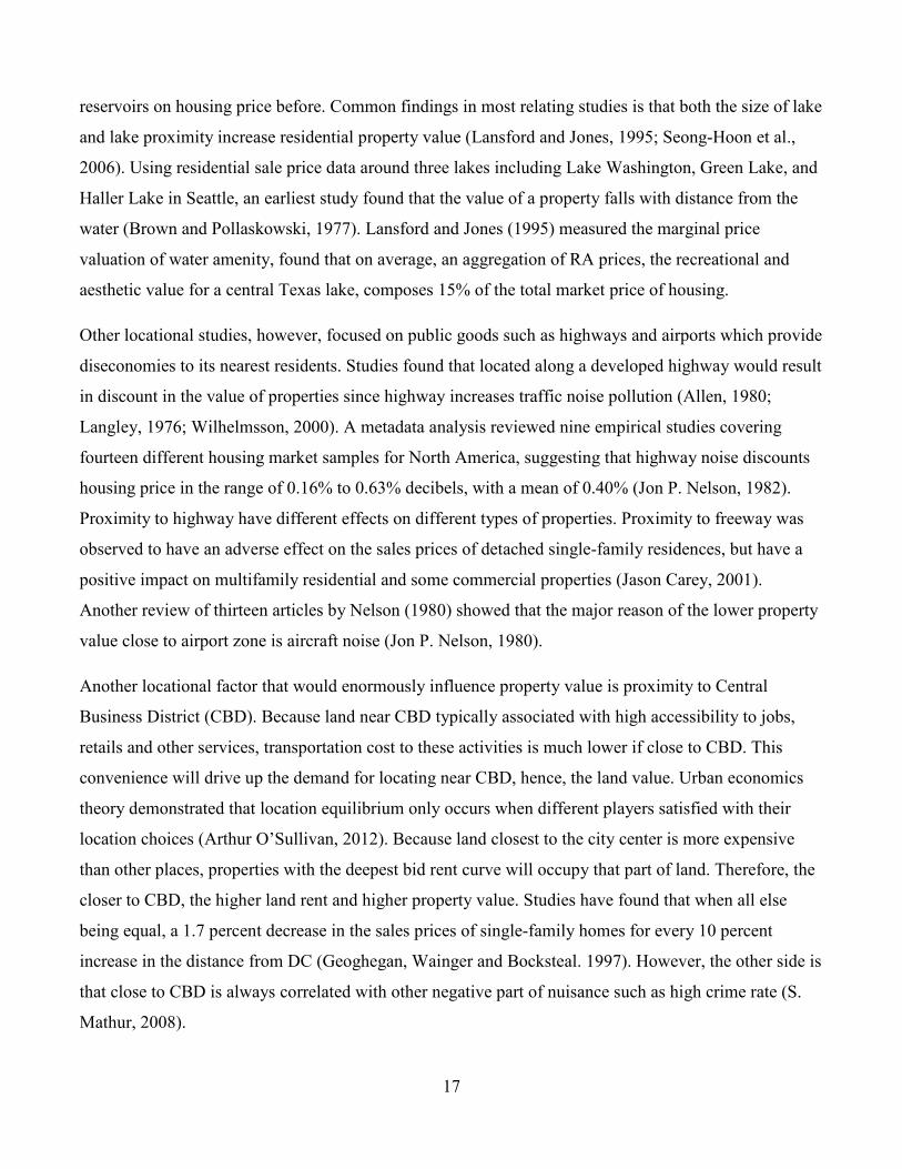
reservoirs on housing price before. Common findings in most relating studies is that both the size of lake
and lake proximity increase residential property value (Lansford and Jones, 1995; Seong-Hoon et al.,
2006). Using residential sale price data around three lakes including Lake Washington, Green Lake, and
Haller Lake in Seattle, an earliest study found that the value of a property falls with distance from the
water (Brown and Pollaskowski, 1977). Lansford and Jones (1995) measured the marginal price
valuation of water amenity, found that on average, an aggregation of RA prices, the recreational and
aesthetic value for a central Texas lake, composes 15% of the total market price of housing.
Other locational studies, however, focused on public goods such as highways and airports which provide
diseconomies to its nearest residents. Studies found that located along a developed highway would result
in discount in the value of properties since highway increases traffic noise pollution (Allen, 1980;
Langley, 1976; Wilhelmsson, 2000). A metadata analysis reviewed nine empirical studies covering
fourteen different housing market samples for North America, suggesting that highway noise discounts
housing price in the range of 0.16% to 0.63% decibels, with a mean of 0.40% (Jon P. Nelson, 1982).
Proximity to highway have different effects on different types of properties. Proximity to freeway was
observed to have an adverse effect on the sales prices of detached single-family residences, but have a
positive impact on multifamily residential and some commercial properties (Jason Carey, 2001).
Another review of thirteen articles by Nelson (1980) showed that the major reason of the lower property
value close to airport zone is aircraft noise (Jon P. Nelson, 1980).
Another locational factor that would enormously influence property value is proximity to Central
Business District (CBD). Because land near CBD typically associated with high accessibility to jobs,
retails and other services, transportation cost to these activities is much lower if close to CBD. This
convenience will drive up the demand for locating near CBD, hence, the land value. Urban economics
theory demonstrated that location equilibrium only occurs when different players satisfied with their
location choices (Arthur O’Sullivan, 2012). Because land closest to the city center is more expensive
than other places, properties with the deepest bid rent curve will occupy that part of land. Therefore, the
closer to CBD, the higher land rent and higher property value. Studies have found that when all else
being equal, a 1.7 percent decrease in the sales prices of single-family homes for every 10 percent
increase in the distance from DC (Geoghegan, Wainger and Bocksteal. 1997). However, the other side is
that close to CBD is always correlated with other negative part of nuisance such as high crime rate (S.
Mathur, 2008).
18
2.3 SUMMARY OF LITERATURE REVIEW
This Chapter reviewed studies on TOD and other factors influencing residential property value. Based
on these, a brief summary of key points are as follows:
• Transit-Oriented Development is typically composed of transit accessibility, mixed land use near
transit station and pedestrian oriented design. These components working together to enhance the
accessibility and convenience to different types of activities therefore will increase the
willingness to pay for the nearby properties.
• Extensive body of literatures corroborate the statement that transit adjacency have premium
effects on residential property value. However, the degree of relative importance of station
proximity on housing price varies, which is affected by other variables change, their different
settings, target market, as well as transit types.
• There are still a small part of literatures found no significant relationship between TOD and
property value increase. But using interaction-term analysis, proximity to station becomes
significant to housing price. This means the effect of TOD is sometimes conditional upon other
environments.
• Most previous literatures focus more on a narrow part of TOD, i.e., transit accessibility.
However, other components like mixed land use and walkable pedestrian design have not been
mentioned a lot.
• Most previous works applied cross-sectional Hedonic Regression Analysis approach, only
measuring the impact of TOD on properties located at different distance to station. However,
longitudinal approach providing more evidence of causality are less used compared with cross-
sectional studies.
• Few study did similar research in Seattle metropolitan area, thus how TOD impact residential
property value in this area is still an open question.
• Besides TOD-related variables, existing studies measured variables in three categories: 1)
physical structure of the building, like size, age, bedrooms; 2) Social-economic characteristics,
such as race, age, and income; 3) Locational factors, like close to CBD, close to open space and
highways. These studies help to build a conceptual model of factors affecting property values
19
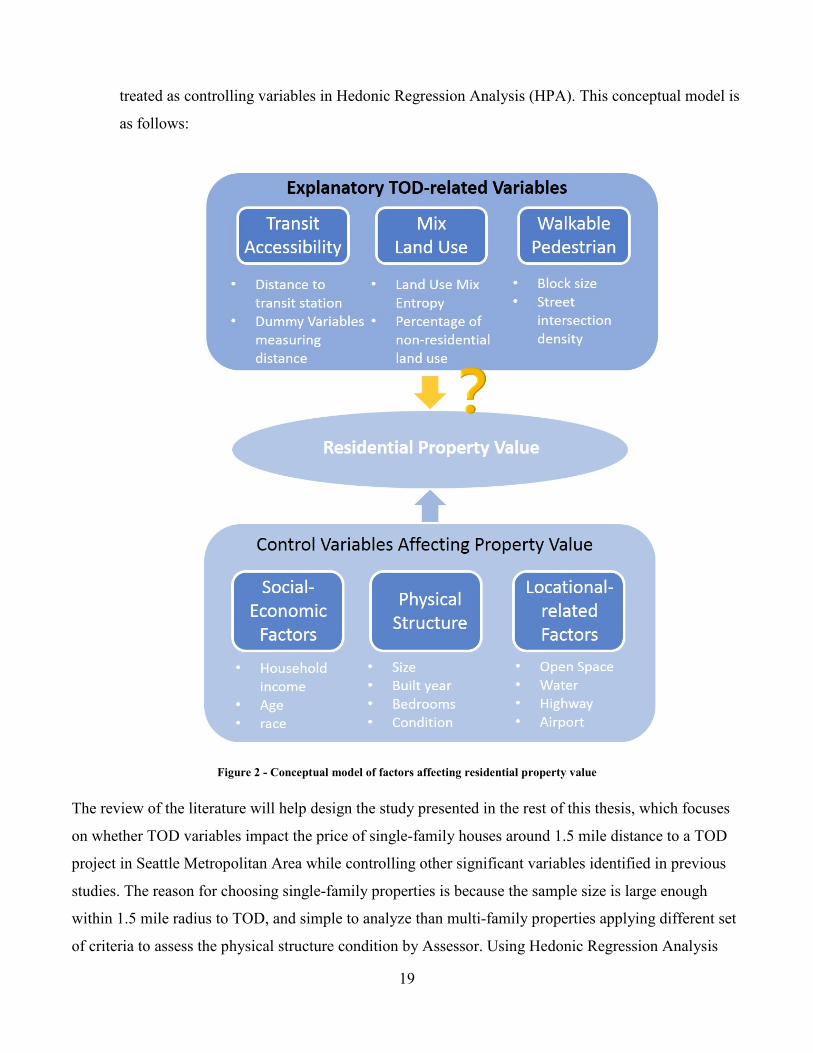
treated as controlling variables in Hedonic Regression Analysis (HPA). This conceptual model is
as follows:
Figure 2 - Conceptual model of factors affecting residential property value
The review of the literature will help design the study presented in the rest of this thesis, which focuses
on whether TOD variables impact the price of single-family houses around 1.5 mile distance to a TOD
project in Seattle Metropolitan Area while controlling other significant variables identified in previous
studies. The reason for choosing single-family properties is because the sample size is large enough
within 1.5 mile radius to TOD, and simple to analyze than multi-family properties applying different set
of criteria to assess the physical structure condition by Assessor. Using Hedonic Regression Analysis

20
(HPA), this study will evaluate whether people are more willing to pay a premium near station area, and
how much premium they would like to pay if living closer to a transit station under Transit-Oriented
Development rather than an otherwise comparable house outside a limited distance to station. Also, this
study will analyze housing sale price before, during, and after the TOD construction to provide more
statistical evidence of causal relationship between TOD and residential property value.
21
CHAPTER 3 STUDY AREA
3.1 STUDY AREA SELECTION CRITERIA
The criteria for study area selection is that: 1) A large real TOD project has been took into effect for a
long time, at least for 10 years; 2) There are a great many residential properties within one and a half
mile radius of the TOD station before and after TOD implementation; 3) The property value have
changed overtime; 4) Available data. At first, the Link light rail stations in city of Seattle served as the
probable study areas. However, some conditions may hinder choosing light rail stations in Seattle as
study area. First, the Link light rail service in Seattle was opened in 2009, the time span do not meet the
first criteria. Second, for most Link light rail stations with significant single-family residences within
one and a half mile radius of station, such as Bacon hill and Othello, even if did have TOD liked station
area plan in 1989, real large TOD project began construction too late, and most are still in construction
now. Third, within one and a half mile radius of station, besides the study station, there are other Link
light rail stations with TOD-liked components which makes difficult to control the effects of other
stations. Thus, I began to search real large TOD project in King County website. In King County,
completed TOD projects include Village at Overlake, Renton Transit Center, Downtown Redmond
Transit Center, and Northgate. All of them are served by King County Metro Transit (KC Metro). The
transit center of downtown Redmond was officially opened in February, 2008, therefore does not meet
the time span limitation. In addition, it is also difficult to meet the second criteria. Same condition is for
another TOD project -Village at Overlake. Northgate is either not an ideal place for doing this analysis
because the transit service was completed late till 2009. Thus, Renton Transit Center, opened and started
TOD construction in 1996, served as the study area of this analysis. The target properties are single-
family properties within 1.5 mile distance to the Renton Transit Center as single-families are easier to
analysis and are with enough sample size.
3.2 STUDY AREA DESCRIPTION
22
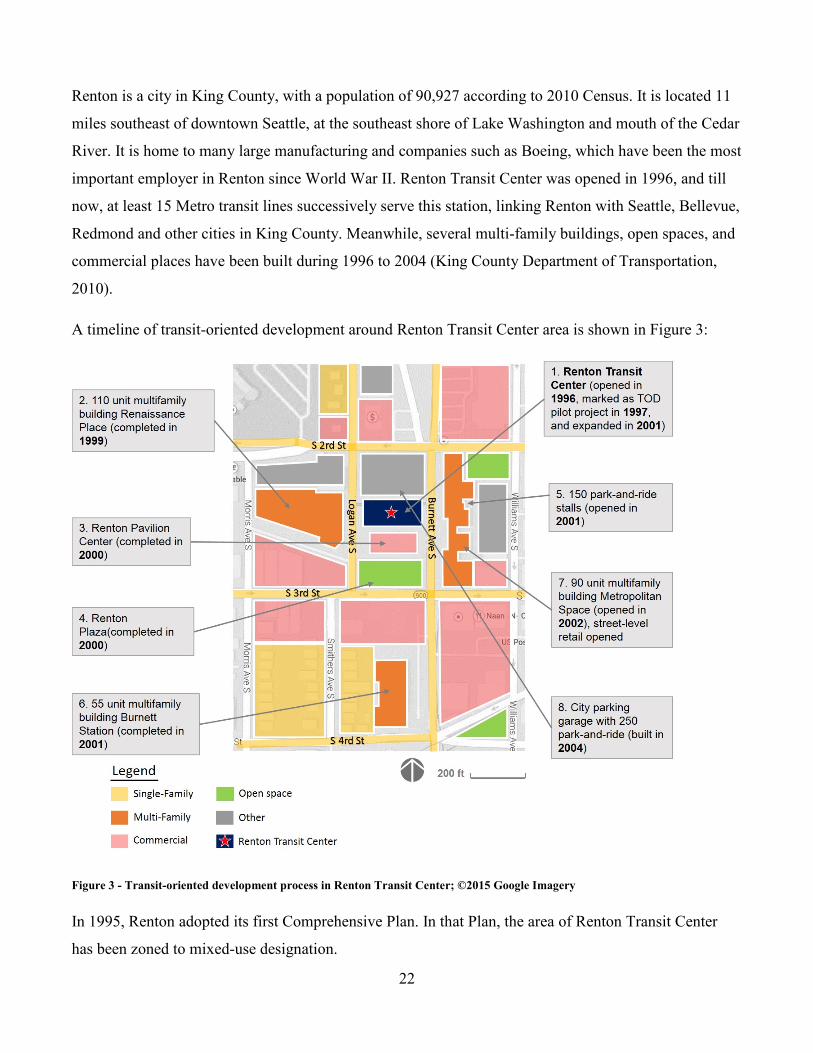
Renton is a city in King County, with a population of 90,927 according to 2010 Census. It is located 11
miles southeast of downtown Seattle, at the southeast shore of Lake Washington and mouth of the Cedar
River. It is home to many large manufacturing and companies such as Boeing, which have been the most
important employer in Renton since World War II. Renton Transit Center was opened in 1996, and till
now, at least 15 Metro transit lines successively serve this station, linking Renton with Seattle, Bellevue,
Redmond and other cities in King County. Meanwhile, several multi-family buildings, open spaces, and
commercial places have been built during 1996 to 2004 (King County Department of Transportation,
2010).
A timeline of transit-oriented development around Renton Transit Center area is shown in Figure 3:
Figure 3 - Transit-oriented development process in Renton Transit Center; ©2015 Google Imagery
In 1995, Renton adopted its first Comprehensive Plan. In that Plan, the area of Renton Transit Center
has been zoned to mixed-use designation.
23
In 1996, the City negotiated with King County Metro over the location of a new transit center. Then,
Renton Transit Center opened at 2nd Avenue and Logan Street as an interim transit hub to provide
downtown Renton with easy transit access to other part of King County. Meanwhile, the City recruited
Don Dally of Dally Properties, a private company, to support mixed-use development around station
area.
Shortly after a year, in 1997, King County Metro decided to mark Renton transit center a location for
pilot TOD project.
In 1999, Dally Properties completed building the first multifamily building, namely Renaissance Place, a
110-unit apartment complex, near the Transit Center area. In the same year, King County and Dally
made an agreement of joint development of TOD project.
In 2000, Renton Piazza, a green plaza adjacent to the transit center was completed. Around the same
time, another project used for banquet venue, Renton Pavilion Center, was then completed near transit
center.
In 2001, King County Metro Transit renovated and expanded the Renton Transit Center to include
additional parking, a plaza, new bus layover, loading areas and street intersection improvements. The
work also includes new paving, shelters, landscaping and other passenger and pedestrian improvement
as joint-development projects of King County Metro Transit and City of Renton, costs for approximately
$4.4 million (King County Department of Transportation, 2010). In the same year, Dally Property built
the second multifamily project – Burnett Station, a 55-unit apartment complex near the transit center.
Meanwhile, Dally Homes decided to develop Metropolitan Place Apartment, which has 90 apartments
above a two-story garage with 240 parking stalls. King County leases 150 of the parking stalls for park-
and-ride uses for 30 years, opened in 2001. King County Metro Transit also made an agreement with
Dally Homes, permitted many goals to be met in TOD development while King County created new
park-and-ride capacity and Dally created mixed-use affordable housing (King County Department of
Transportation, 2010).
In 2002, the newly expanded transit center opened, and 90 apartments of Metropolitan Place opened
shortly after. In the same year, 4,000 square feet of street-level retail space built into the northwest
corner of Metropolitan Place.
24
In 2004, city of Renton built a freestanding city parking garage with 250 park-and-ride spaces next to
the transit center.
In sum, the transit-oriented developent in Renton Transit Center was started in approximately 1996, with
at least a time span of around 9 years (from 1996 to 2004) to complete all TOD components. Therefore,
in this analysis, the years before 1996 are treated as before-TOD, the years from 1996 to 2004 are during
TOD construction, and the years after 2004 are treated as post-TOD.
25
CHAPTER 4 DATA AND METHODOLOGY
4.1 METHODOLOGY
Hedonic price method is the most commonly used method to study the marginal implicit housing price
as affected by each attribute. In 1966, Lancaster proposed an approach in his paper that the output for a
good are a collection of more than one characteristics rather than a homogenous type (Lancaster, 1966).
In 1974, Rosen derive implicit attribute prices for multi-attribute goods using Hedonic Price Method.
The Hedonic price method assumes that the characteristics which affecting housing price can be
decomposed thereby can treat each of them separately in order to estimate prices or elasticity for each of
them (Rosen, 1974). Housing prices are affected by their combination of different characteristics.
Among these characters, as for this study, TOD is an important part. Besides TOD, there are also other
kinds of factors, including locational factors, physical structure factors, and social-economic factors that
affect housing price. Therefore, using Hedonic method can disentangle the effect of different attributes
of housing price in order to obtain the marginal implicit price of TOD factors.
In this study, rather than using a simple linear functional form, a semi-logarithmic function form is used.
Unlike the simple linear functional form measuring the absolute amount of dependent variable change as
driven by per unit increase or decrease of independent variables, the semi-logarithmic function estimates
the percentage change of dependent variable as according to a unit change of different independent
variables. Thus, in order to compare the result of this study with other studies, the “Percentage effects”
of semi-logarithmic function is better than a simple linear functional form.
A typical semi-log linear form of Hedonic regression method is used in this study:
ln � = �� +� �� + ��� +���� +���� +���� + �
Where�� is a constant, P is the single family property sales price in 1.5 mile buffer from Renton Transit
Center, �� are the social-economic variables; �� are the TOD related variables; �� are other locational
related variables; �� are physical characteristics of the property; �� are time-series dummy variables
capturing different years of transactions.
26
4.1.1 TWO TIME-SERIES MODELS
In order to answer the research question that to what extent a completed TOD project fulfilled the role of
capitalizing residential property value both in time and space, two basic time-series models are built
using the typical semi-log form HPA method illustrated before.
Since all the transaction prices were adjusted to 2015 dollar price before analysis using S&P/ Case-
Shiller Seattle Home Price Index which only covers a time span between 1990 and 2015, the total time
period chosen is from 1990 to 2015 for this time-series analysis which includes 6 years before TOD
construction (1990-1995), 9 years during TOD construction (1996-2004), and 11 years after that (2005-
2015).
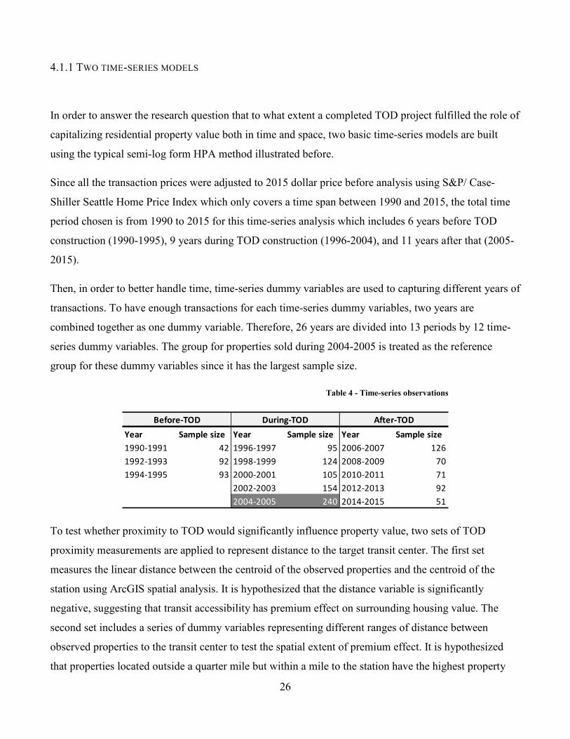
Then, in order to better handle time, time-series dummy variables are used to capturing different years of
transactions. To have enough transactions for each time-series dummy variables, two years are
combined together as one dummy variable. Therefore, 26 years are divided into 13 periods by 12 time-
series dummy variables. The group for properties sold during 2004-2005 is treated as the reference
group for these dummy variables since it has the largest sample size.
Table 4 - Time-series observations
To test whether proximity to TOD would significantly influence property value, two sets of TOD
proximity measurements are applied to represent distance to the target transit center. The first set
measures the linear distance between the centroid of the observed properties and the centroid of the
station using ArcGIS spatial analysis. It is hypothesized that the distance variable is significantly
negative, suggesting that transit accessibility has premium effect on surrounding housing value. The
second set includes a series of dummy variables representing different ranges of distance between
observed properties to the transit center to test the spatial extent of premium effect. It is hypothesized
that properties located outside a quarter mile but within a mile to the station have the highest property
Year Sample size Year Sample size Year Sample size
1990-1991 42 1996-1997 95 2006-2007 126
1992-1993 92 1998-1999 124 2008-2009 70
1994-1995 93 2000-2001 105 2010-2011 71
2002-2003 154 2012-2013 92
2004-2005 240 2014-2015 51
After-TODDuring-TODBefore-TOD
27
value because station area properties (properties within a quarter mile distance) are often associated with
TOD-related nuisances such as congestion and noise. All transaction properties are divided into four
categories: those located within 0.25 mile to the target station; located within 0.25-0.5 mile; within 0.5-1
mile; and within 1-1.5 mile to the target station. Three distance dummy variables are used to categorize
them. It is not possible to add all these two kind of variables in a particular regression model because of
the collinearity, therefore two models are built separately, and each includes a kind of measurement:
Model 1: ln � = �� +∑���� + ����_�� + ∑���� + ��
Model 2: ln � = �! +∑ ���� + ∑"�����_�#$$%� + ∑ ���� + �!
Where �� are other variables (including social-economic, locational, physical structure and other TOD
related variables) except for the variable of distance to transit center; ���_�� is the distance between
the observed properties and the transit center; ����_�#$$%� are the three dummy variables indicating
four distance bands. ��, e, "�, and �� are coefficients, �� and �! are constants; �� and �! are error terms.
4.1.2 BEFORE-DURING-AFTER MODELS
Then, in order to answer the question that whether housing price show any difference before and after
TOD took into effect, the before-during-after analysis is used to capture the differences. Six models
representing before, during, and after the implementation of TOD are then conducted in this study using
the basic form of Hedonic model. The first set of three includes distance to TOD as an independent
variable, the last set of three measures distance by distance dummy variables.
According to the background of study area TOD development in Chapter 3, the project was started in the
year of 1996, and spent for about 9 years (from 1996 to 2004) to finish all the TOD components (transit
accessibility, mixed land use and pedestrian-oriented design). Therefore, properties sold before 1996 are
used for pre-TOD models, those sold during 1996-2004 are used for during-TOD models, and properties
sold on 2005 and after are used for post-TOD models.
28
A more detailed description of variables and data source are in the following Chapter 4.2.
Model 3: Properties sold during 1990-1995 (Pre-TOD) – using distance to TOD
Model 6: Properties sold during 1990-1995 (Pre-TOD) – using distance dummy variables
Model 4: Properties sold during 1996-2004 (Under-construction) – using distance to TOD
Model 7: Properties sold during 1996-2004 (Under-construction) – using distance dummy variables
Model 5: Properties sold during 2004-2015 (Post-TOD) – using distance to TOD
Model 8: Properties sold during 2004-2015 (Post-TOD) – using distance dummy variables
4.2 DATA
Based on the conceptual model summarized from extensive body of literatures on housing price
measured by Hedonic Price Analysis method, variables needed for this study are shown in Table 5. Data
for measuring these variables are collected from various sources or calculated in GIS software. The
following are the major types of data:
4.2.1 DATA TYPES
TRANSACTION PRICE DATA
The transaction price data comes from real property sales data which contains records for sales,
including the sales price, sales date, and principle uses etc. started from 1982 in King County
Department of Assessor (KC Assessor). The field name “major” and “minor” are concatenated to create
PIN code, which is the key attribute to join to GIS parcel file.
RESIDENTIAL BUILDING RECORD DATA
29
The residential building record data contains physical structure records such as building grade, square
footage, year built, condition etc. for each residential building from KC Assessor. This data file is
limited to current status of the building, however the condition of the houses may have changed during
the past years. Therefore, an attribute of “renovation year” in this file is used to pick out properties at
least have not been renovated after the transaction year.
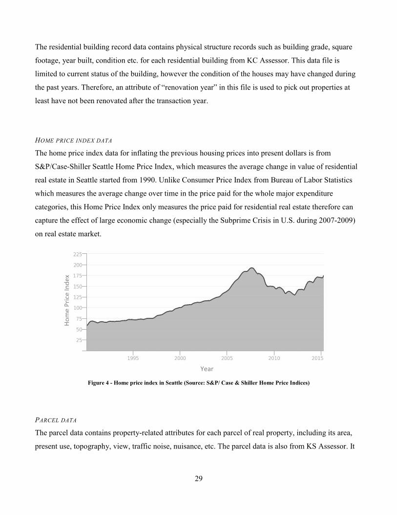
HOME PRICE INDEX DATA
The home price index data for inflating the previous housing prices into present dollars is from
S&P/Case-Shiller Seattle Home Price Index, which measures the average change in value of residential
real estate in Seattle started from 1990. Unlike Consumer Price Index from Bureau of Labor Statistics
which measures the average change over time in the price paid for the whole major expenditure
categories, this Home Price Index only measures the price paid for residential real estate therefore can
capture the effect of large economic change (especially the Subprime Crisis in U.S. during 2007-2009)
on real estate market.
Figure 4 - Home price index in Seattle (Source: S&P/ Case & Shiller Home Price Indices)
PARCEL DATA
The parcel data contains property-related attributes for each parcel of real property, including its area,
present use, topography, view, traffic noise, nuisance, etc. The parcel data is also from KS Assessor. It
Year
Ho
me
Pri
ce I
nd
ex
30
depicts the current condition of the properties but not at the time the properties sold. Thus, using this
data may create some inaccuracy.
VARIOUS OF GIS SHAPEFILE DATA
The dataset also contains an object-oriented GIS layer of study area parcels from King County GIS
Center (KCGIS Center). It provides geometry for spatial analysis and a series of parcel-related
information attached to it. An important attribute for this file is the present use of the parcel, which is
used for calculating land use mix score, percentage of commercial uses and other land use related
variables.
Other GIS data used in this study includes transportation network, lake Washington, river and other bus
stops, all are from KCGIS Center.
SOCIAL-ECONOMIC DATA
The social-economic data are from 2010 Census and American Community Survey (ACS) 5-year
Estimate (2009-2013).
4.2.2 DATA FILTERING
ArcGIS is used to identify properties within 1.5 mile distance from Renton Transit Center and sold
during 1990 to 2015: First, in order to identify single family properties within 1.5 mile distance to the
Transit Center, three criteria are used:
1) The present land use code of the parcel equals to “2”, or “6” (“2” means single-family in residential
use/residential zone; “6” means single-family in commercial or industry zone). Only around 20
properties are in the land use code of “6”. All of these properties are in residential uses according to their
photos, tax roll history, and physical characteristics such as number of bathrooms according to King
County Parcel Viewer 2.0.
31
2) Parcels filtered by step 1) should have only 1 living unit to exclude properties not in single-family
uses.
3) Because the target of this study is only single-family properties within 1.5 mile distance to the transit
center, GIS was used to identify parcels filtered by step 2) are within 1.5 mile buffer from Renton
Transit Center.
Using these three criteria, single-family parcels in the study area were identified. Second, real estate
transaction data were then joined to those single-family parcels. Using the attribute of “document date”,
single-family properties sold during 1990 to 2015 were picked out. After that, residential building record
data were joined to single-family parcels sold during 1990 to 2015. As physical structure data are limited
to current condition, “renovation year” in the residential building record data file was used to identify
properties which still maintain physical characteristics at the transaction time. Therefore, properties
having “renovation year” larger than “transaction year” were excluded. Other kind of information like
social-economic data were also added into the GIS database and matched to each single-family parcels.
Land use related data were calculated first using GIS and then also matched to parcels.
Properties in the dataset with missing data or obvious data mistake were then excluded. A total number
of 1,355 single-family transactions were identified within the time span from 1990 to 2015 after
removing those with sales price equal to “0” meaning mere transferring interest and those having
obvious errors made by record (e.g. a normal condition single family house sold for only 149 dollars in
recent years; properties with “null” records in most physical characteristics columns).
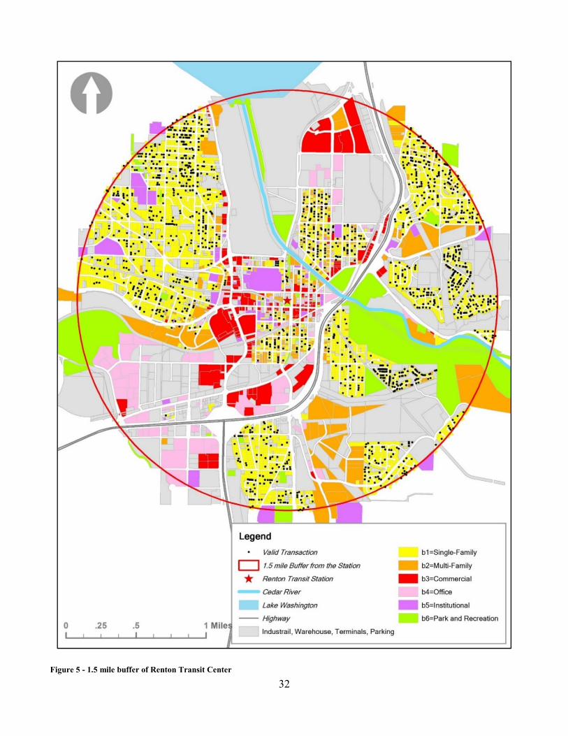
32
Figure 5 - 1.5 mile buffer of Renton Transit Center
33
4.2.3 DATA BY CATEGORY
DEPENDENT VARIABLE – LOGARITHM OF ADJUSTED TRANSACTION PRICE
The transaction price data is from KS Assessor. Considering the inflation due to decline in the value of
money, transaction price in previous year dollar value are inflated to dollar value in 2015 using annual
S&P/Case-Shiller Seattle Home Price Index. The calculation function is as follows:
�' =�( × (+'/+()
Where �' is the value of dollar in present year; �( is the dollar value in past year; +' is the Home Price
Index in present year; +( is the Home Price Index in past year.
CONTROLLING INDEPENDENT VARIABLE – PHYSICAL STRUCTURE VARIABLES
The physical structure controlling variables entering in the model are building grade, square footage of
finished area above floor, square footage of total basement, number of bedrooms, age of the structure,
logarithm of age square, condition of the structure, and number of stories. This series of data are from
residential building record from KC Assessor. Since the relation between age of the structure and the
housing price is often not linear, and sometimes historic houses are more expensive than moderately
new houses, the age square is added into the physical structure variables. In order to reduce severe
collinearity in models, age square is transformed into logarithm form first and added together with age
into the regression model.
CONTROLLING INDEPENDENT VARIABLE – LOCATIONAL CHARACTERISTICS
The locational characteristics include distance to highway, distance to Lake Washington, distance to
Cedar River, distance to nearest park, and distance to other bus stops, dummy variables distinguishing
whether the property has lake view or not, dummy variables capturing whether the property has detected
traffic noise or not, dummy variables capturing whether the property has other kind of nuisance or not.
Distance to CBD was originally included in it, but eliminated then subject to severe collinearity of the
data.
34
All the distance data are calculated in ArcGIS using data from KCGIS Center. The highway data is from
the dataset of Transportation Network (TNET) in King County GIS Portal, only picking out two types of
roads: highways and expressways. The bus stops data (not containing Renton Transit Center) are a
merge of Metro bus stops as well as bus stops served by Sound Transit, another transit agency providing
regional express service in the study area. The GIS data of Lake Washington, Cedar River and Parks are
also from KCGIS Center.
The view of Lake Washington, traffic noise, and other nuisance data are within parcel record data from
KS Assessor. Properties are assigned “1” and “0” indicating whether they have these condition or not.
CONTROLLING INDEPENDENT VARIABLE – SOCIAL-ECONOMIC FACTORS
The social-economic variables, including race percentage, median age, and median income, are available
from Census and American Community Survey. While race and median age are at block level, median
income is at block-group level.
EXPLANATORY INDEPENDENT VARIABLE – TOD-RELATED VARIABLES
The final most important variables are TOD related. Based on previous study on premium effect of TOD
from Chapter 2, three kinds of important variables are used to capture TOD premium – proximity to
TOD, mixed uses, and pedestrian-oriented design.
To measure proximity to TOD, two sets of models are estimated. The first one uses distance to TOD as
an independent variable, the other uses a set of dummy coding distance variables representing different
distance bands to the Transit Center. Sometimes the effect of proximity to TOD is not as simple as a
linear function because TOD is sometimes associated with negative externalities as Chapter 2 illustrated,
therefore the surrounding housing price will impact from how homebuyers trade-off the advantages and
disadvantages under different circumstances. Another reason is that, sometimes people are willing to pay
similar dollars to two houses, both within a walking distance to the transit station, no matter one of them
is a little closer to the station.
Thus, in many previous studies, other than using distance to TOD as an independent variable, another
way to compare how proximity to TOD affects property value is using a series of dummy coding
variables to test the spatial extent of the price effect of TOD. Various distance bands were tested in
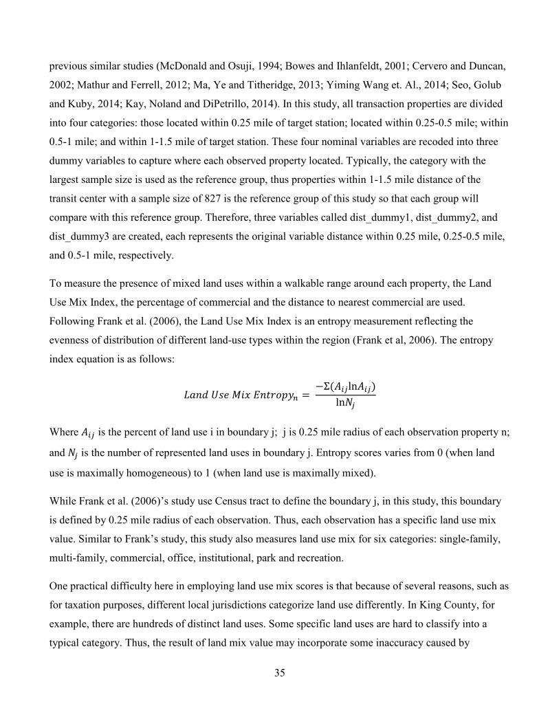
35
previous similar studies (McDonald and Osuji, 1994; Bowes and Ihlanfeldt, 2001; Cervero and Duncan,
2002; Mathur and Ferrell, 2012; Ma, Ye and Titheridge, 2013; Yiming Wang et. Al., 2014; Seo, Golub
and Kuby, 2014; Kay, Noland and DiPetrillo, 2014). In this study, all transaction properties are divided
into four categories: those located within 0.25 mile of target station; located within 0.25-0.5 mile; within
0.5-1 mile; and within 1-1.5 mile of target station. These four nominal variables are recoded into three
dummy variables to capture where each observed property located. Typically, the category with the
largest sample size is used as the reference group, thus properties within 1-1.5 mile distance of the
transit center with a sample size of 827 is the reference group of this study so that each group will
compare with this reference group. Therefore, three variables called dist_dummy1, dist_dummy2, and
dist_dummy3 are created, each represents the original variable distance within 0.25 mile, 0.25-0.5 mile,
and 0.5-1 mile, respectively.
To measure the presence of mixed land uses within a walkable range around each property, the Land
Use Mix Index, the percentage of commercial and the distance to nearest commercial are used.
Following Frank et al. (2006), the Land Use Mix Index is an entropy measurement reflecting the
evenness of distribution of different land-use types within the region (Frank et al, 2006). The entropy
index equation is as follows:
./0����1�"20�3�4%' =−Σ(��7ln��7)
ln87
Where ��7 is the percent of land use i in boundary j; j is 0.25 mile radius of each observation property n;
and 87 is the number of represented land uses in boundary j. Entropy scores varies from 0 (when land
use is maximally homogeneous) to 1 (when land use is maximally mixed).
While Frank et al. (2006)’s study use Census tract to define the boundary j, in this study, this boundary
is defined by 0.25 mile radius of each observation. Thus, each observation has a specific land use mix
value. Similar to Frank’s study, this study also measures land use mix for six categories: single-family,
multi-family, commercial, office, institutional, park and recreation.
One practical difficulty here in employing land use mix scores is that because of several reasons, such as
for taxation purposes, different local jurisdictions categorize land use differently. In King County, for
example, there are hundreds of distinct land uses. Some specific land uses are hard to classify into a
typical category. Thus, the result of land mix value may incorporate some inaccuracy caused by

36
categorizing process. In this study, hundreds of distinct land uses are classified into 6 categories. Each
category and its corresponding land use code from King County parcel file are shown in Appendix C –
Land Use Category, Present Land Use Code and Code Definition.
In addition, a typical problem for measuring land use mix through this way is that high land use entropy
score sometimes do not imply high level of land use mix because different land use configuration
matters a lot. For example, the following two area would achieve the same mixed use scores:
A = ½ Single-family + ½ Multi-family
B = 1/6 Single-family + 1/6 Multi-family + 1/6 Commercial + 1/6 Office + 1/6 Institutional + 1/6 Open
Space/Recreation
The area A and B both have the land use mix entropy score of 1.0, but the area B is obviously highly
mixed compared with the area A with only residential uses.
Given the potential mistakes caused by the mix use entropy measurement, another variable used to
reduce such error is the percentage of commercial uses around a 0.25 mile buffer from the observation
calculated in GIS using Parcel data file.
As for the reason why mix use may improve property value is because of the increase in proximity and
convenience to daily activities, therefore this study also use distance to the nearest commercial uses as a
variable to measure whether close to commercial has advantage on housing value.
To measure a walkable street design, as most previous studies focused on block size, the size of block in
which the observation property located is also an independent variable in this study. The block size data
is also calculated in ArcGIS software.
EXPLANATORY INDEPENDENT VARIABLE – TIME-SERIES VARIABLES
Then, in Model 1 & Model 2, 12 time dummy variables are used to capture different years of
transactions, using properties sold during 2004-2005 as the reference group.
The description of variables and their data source are as follows:
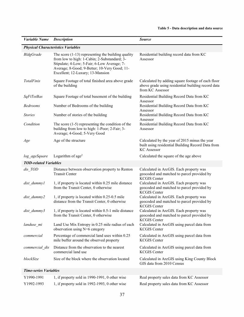
37
Table 5 - Data description and data source
Variable Name Description Source
Physical Characteristics Variables
BldgGrade The score (1-13) representing the building quality from low to high: 1-Cabin; 2-Substandard; 3-Stipulate; 4-Low; 5-Fair; 6-Low Average; 7-Average; 8-Good; 9-Better; 10-Very Good; 11-Excellent; 12-Luxury; 13-Mansion
Residential building record data from KC Assessor
TotalFinis Square Footage of total finished area above grade of the building
Calculated by adding square footage of each floor above grade using residential building record data from KC Assessor
SqFtTotBas Square Footage of total basement of the building Residential Building Record Data from KC Assessor
Bedrooms Number of Bedrooms of the building Residential Building Record Data from KC Assessor
Stories Number of stories of the building Residential Building Record Data from KC Assessor
Condition The score (1-5) representing the condition of the building from low to high: 1-Poor; 2-Fair; 3-Average; 4-Good; 5-Very Good
Residential Building Record Data from KC Assessor
Age Age of the structure Calculated by the year of 2015 minus the year built using residential Building Record Data from KC Assessor
log_ageSquare Logarithm of age2 Calculated the square of the age above
TOD-related Variables
dis_TOD Distance between observation property to Renton Transit Center
Calculated in ArcGIS. Each property was geocoded and matched to parcel provided by KCGIS Center
dist_dummy1 1, if property is located within 0.25 mile distance from the Transit Center, 0 otherwise
Calculated in ArcGIS. Each property was geocoded and matched to parcel provided by KCGIS Center
dist_dummy2 1, if property is located within 0.25-0.5 mile distance from the Transit Center, 0 otherwise
Calculated in ArcGIS. Each property was geocoded and matched to parcel provided by KCGIS Center
dist_dummy3 1, if property is located within 0.5-1 mile distance from the Transit Center, 0 otherwise
Calculated in ArcGIS. Each property was geocoded and matched to parcel provided by KCGIS Center
landuse_mi Land Use Mix Entropy in 0.25 mile radius of each observation using N=6 category
Calculated in ArcGIS using parcel data from KCGIS Center
commercial Percentage of commercial land uses within 0.25 mile buffer around the observed property
Calculated in ArcGIS using parcel data from KCGIS Center
commercial_dis Distance from the observation to the nearest commercial land use
Calculated in ArcGIS using parcel data from KCGIS Center
blockSize Size of the block where the observation located Calculated in ArcGIS using King County Block GIS data from 2010 Census
Time-series Variables
Y1990-1991 1, if property sold in 1990-1991, 0 other wise Real property sales data from KC Assessor
Y1992-1993 1, if property sold in 1992-1993, 0 other wise Real property sales data from KC Assessor
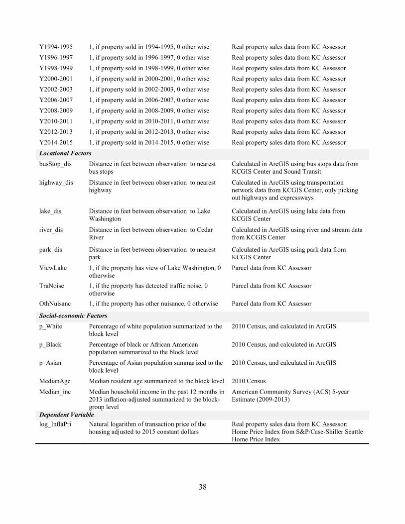
38
Y1994-1995 1, if property sold in 1994-1995, 0 other wise Real property sales data from KC Assessor
Y1996-1997 1, if property sold in 1996-1997, 0 other wise Real property sales data from KC Assessor
Y1998-1999 1, if property sold in 1998-1999, 0 other wise Real property sales data from KC Assessor
Y2000-2001 1, if property sold in 2000-2001, 0 other wise Real property sales data from KC Assessor
Y2002-2003 1, if property sold in 2002-2003, 0 other wise Real property sales data from KC Assessor
Y2006-2007 1, if property sold in 2006-2007, 0 other wise Real property sales data from KC Assessor
Y2008-2009 1, if property sold in 2008-2009, 0 other wise Real property sales data from KC Assessor
Y2010-2011 1, if property sold in 2010-2011, 0 other wise Real property sales data from KC Assessor
Y2012-2013 1, if property sold in 2012-2013, 0 other wise Real property sales data from KC Assessor
Y2014-2015 1, if property sold in 2014-2015, 0 other wise Real property sales data from KC Assessor
Locational Factors
busStop_dis Distance in feet between observation to nearest bus stops
Calculated in ArcGIS using bus stops data from KCGIS Center and Sound Transit
highway_dis Distance in feet between observation to nearest highway
Calculated in ArcGIS using transportation network data from KCGIS Center, only picking out highways and expressways
lake_dis Distance in feet between observation to Lake Washington
Calculated in ArcGIS using lake data from KCGIS Center
river_dis Distance in feet between observation to Cedar River
Calculated in ArcGIS using river and stream data from KCGIS Center
park_dis Distance in feet between observation to nearest park
Calculated in ArcGIS using park data from KCGIS Center
ViewLake 1, if the property has view of Lake Washington, 0 otherwise
Parcel data from KC Assessor
TraNoise 1, if the property has detected traffic noise, 0 otherwise
Parcel data from KC Assessor
OthNuisanc 1, if the property has other nuisance, 0 otherwise Parcel data from KC Assessor
Social-economic Factors
p_White Percentage of white population summarized to the block level
2010 Census, and calculated in ArcGIS
p_Black Percentage of black or African American population summarized to the block level
2010 Census, and calculated in ArcGIS
p_Asian Percentage of Asian population summarized to the block level
2010 Census, and calculated in ArcGIS
MedianAge Median resident age summarized to the block level 2010 Census
Median_inc Median household income in the past 12 months in 2013 inflation-adjusted summarized to the block-group level
American Community Survey (ACS) 5-year Estimate (2009-2013)
Dependent Variable
log_InflaPri Natural logarithm of transaction price of the housing adjusted to 2015 constant dollars
Real property sales data from KC Assessor; Home Price Index from S&P/Case-Shiller Seattle Home Price Index
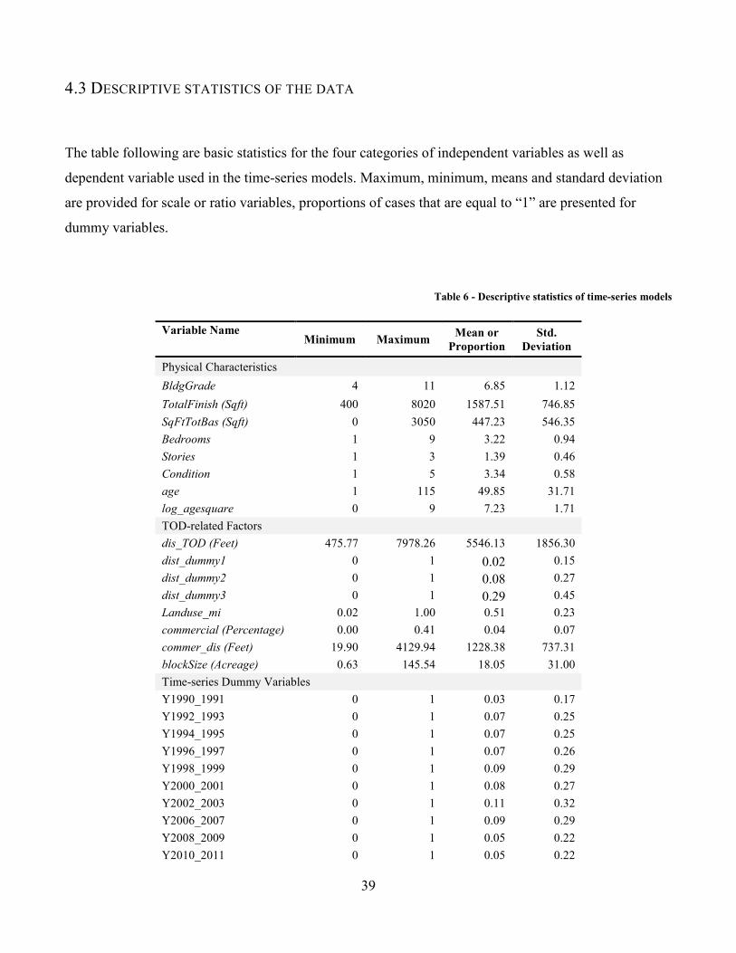
39
4.3 DESCRIPTIVE STATISTICS OF THE DATA
The table following are basic statistics for the four categories of independent variables as well as
dependent variable used in the time-series models. Maximum, minimum, means and standard deviation
are provided for scale or ratio variables, proportions of cases that are equal to “1” are presented for
dummy variables.
Table 6 - Descriptive statistics of time-series models
Variable Name Minimum Maximum
Mean or
Proportion
Std.
Deviation
Physical Characteristics
BldgGrade 4 11 6.85 1.12
TotalFinish (Sqft) 400 8020 1587.51 746.85
SqFtTotBas (Sqft) 0 3050 447.23 546.35
Bedrooms 1 9 3.22 0.94
Stories 1 3 1.39 0.46
Condition 1 5 3.34 0.58
age 1 115 49.85 31.71
log_agesquare 0 9 7.23 1.71
TOD-related Factors
dis_TOD (Feet) 475.77 7978.26 5546.13 1856.30
dist_dummy1 0 1 0.02 0.15
dist_dummy2 0 1 0.08 0.27
dist_dummy3 0 1 0.29 0.45
Landuse_mi 0.02 1.00 0.51 0.23
commercial (Percentage) 0.00 0.41 0.04 0.07
commer_dis (Feet) 19.90 4129.94 1228.38 737.31
blockSize (Acreage) 0.63 145.54 18.05 31.00
Time-series Dummy Variables
Y1990_1991 0 1 0.03 0.17
Y1992_1993 0 1 0.07 0.25
Y1994_1995 0 1 0.07 0.25
Y1996_1997 0 1 0.07 0.26
Y1998_1999 0 1 0.09 0.29
Y2000_2001 0 1 0.08 0.27
Y2002_2003 0 1 0.11 0.32
Y2006_2007 0 1 0.09 0.29
Y2008_2009 0 1 0.05 0.22
Y2010_2011 0 1 0.05 0.22
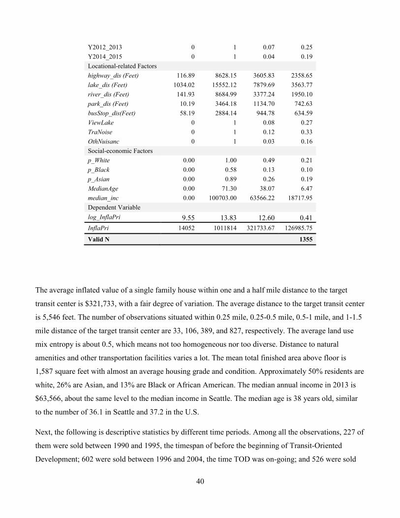
40
Y2012_2013 0 1 0.07 0.25
Y2014_2015 0 1 0.04 0.19
Locational-related Factors
highway_dis (Feet) 116.89 8628.15 3605.83 2358.65
lake_dis (Feet) 1034.02 15552.12 7879.69 3563.77
river_dis (Feet) 141.93 8684.99 3377.24 1950.10
park_dis (Feet) 10.19 3464.18 1134.70 742.63
busStop_dis(Feet) 58.19 2884.14 944.78 634.59
ViewLake 0 1 0.08 0.27
TraNoise 0 1 0.12 0.33
OthNuisanc 0 1 0.03 0.16
Social-economic Factors
p_White 0.00 1.00 0.49 0.21
p_Black 0.00 0.58 0.13 0.10
p_Asian 0.00 0.89 0.26 0.19
MedianAge 0.00 71.30 38.07 6.47
median_inc 0.00 100703.00 63566.22 18717.95
Dependent Variable
log_InflaPri 9.55 13.83 12.60 0.41
InflaPri 14052 1011814 321733.67 126985.75
Valid N 1355
The average inflated value of a single family house within one and a half mile distance to the target
transit center is $321,733, with a fair degree of variation. The average distance to the target transit center
is 5,546 feet. The number of observations situated within 0.25 mile, 0.25-0.5 mile, 0.5-1 mile, and 1-1.5
mile distance of the target transit center are 33, 106, 389, and 827, respectively. The average land use
mix entropy is about 0.5, which means not too homogeneous nor too diverse. Distance to natural
amenities and other transportation facilities varies a lot. The mean total finished area above floor is
1,587 square feet with almost an average housing grade and condition. Approximately 50% residents are
white, 26% are Asian, and 13% are Black or African American. The median annual income in 2013 is
$63,566, about the same level to the median income in Seattle. The median age is 38 years old, similar
to the number of 36.1 in Seattle and 37.2 in the U.S.
Next, the following is descriptive statistics by different time periods. Among all the observations, 227 of
them were sold between 1990 and 1995, the timespan of before the beginning of Transit-Oriented
Development; 602 were sold between 1996 and 2004, the time TOD was on-going; and 526 were sold
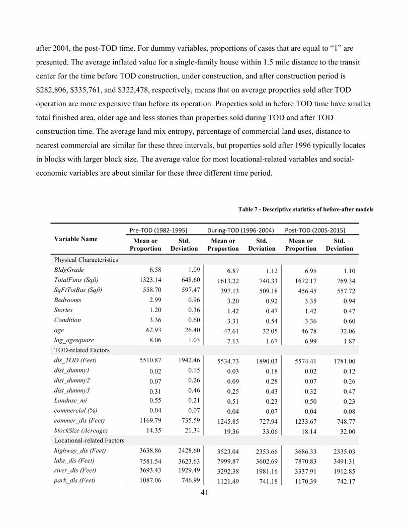
41
after 2004, the post-TOD time. For dummy variables, proportions of cases that are equal to “1” are
presented. The average inflated value for a single-family house within 1.5 mile distance to the transit
center for the time before TOD construction, under construction, and after construction period is
$282,806, $335,761, and $322,478, respectively, means that on average properties sold after TOD
operation are more expensive than before its operation. Properties sold in before TOD time have smaller
total finished area, older age and less stories than properties sold during TOD and after TOD
construction time. The average land mix entropy, percentage of commercial land uses, distance to
nearest commercial are similar for these three intervals, but properties sold after 1996 typically locates
in blocks with larger block size. The average value for most locational-related variables and social-
economic variables are about similar for these three different time period.
Table 7 - Descriptive statistics of before-after models
Variable Name
Pre-TOD (1982-1995) During-TOD (1996-2004) Post-TOD (2005-2015)
Mean or
Proportion
Std.
Deviation
Mean or
Proportion
Std.
Deviation
Mean or
Proportion
Std.
Deviation
Physical Characteristics
BldgGrade 6.58 1.09 6.87 1.12 6.95 1.10
TotalFinis (Sqft) 1323.14 648.60 1613.22 740.33 1672.17 769.34
SqFtTotBas (Sqft) 558.70 597.47 397.13 509.18 456.45 557.72
Bedrooms 2.99 0.96 3.20 0.92 3.35 0.94
Stories 1.20 0.36 1.42 0.47 1.42 0.47
Condition 3.36 0.60 3.31 0.54 3.36 0.60
age 62.93 26.40 47.61 32.05 46.78 32.06
log_agesquare 8.06 1.03 7.13 1.67 6.99 1.87
TOD-related Factors
dis_TOD (Feet) 5510.87 1942.46 5534.73 1890.03 5574.41 1781.00
dist_dummy1 0.02 0.15 0.03 0.18 0.02 0.12
dist_dummy2 0.07 0.26 0.09 0.28 0.07 0.26
dist_dummy3 0.31 0.46 0.25 0.43 0.32 0.47
Landuse_mi 0.55 0.21 0.51 0.23 0.50 0.23
commercial (%) 0.04 0.07 0.04 0.07 0.04 0.08
commer_dis (Feet) 1169.79 735.59 1245.85 727.94 1233.67 748.77
blockSize (Acreage) 14.35 21.34 19.36 33.06 18.14 32.00
Locational-related Factors
highway_dis (Feet) 3638.86 2428.60 3523.04 2353.66 3686.33 2335.03
lake_dis (Feet) 7581.54 3623.63 7999.87 3602.69 7870.83 3491.31
river_dis (Feet) 3693.43 1929.49 3292.38 1981.16 3337.91 1912.85
park_dis (Feet) 1087.06 746.99 1121.49 741.18 1170.39 742.17
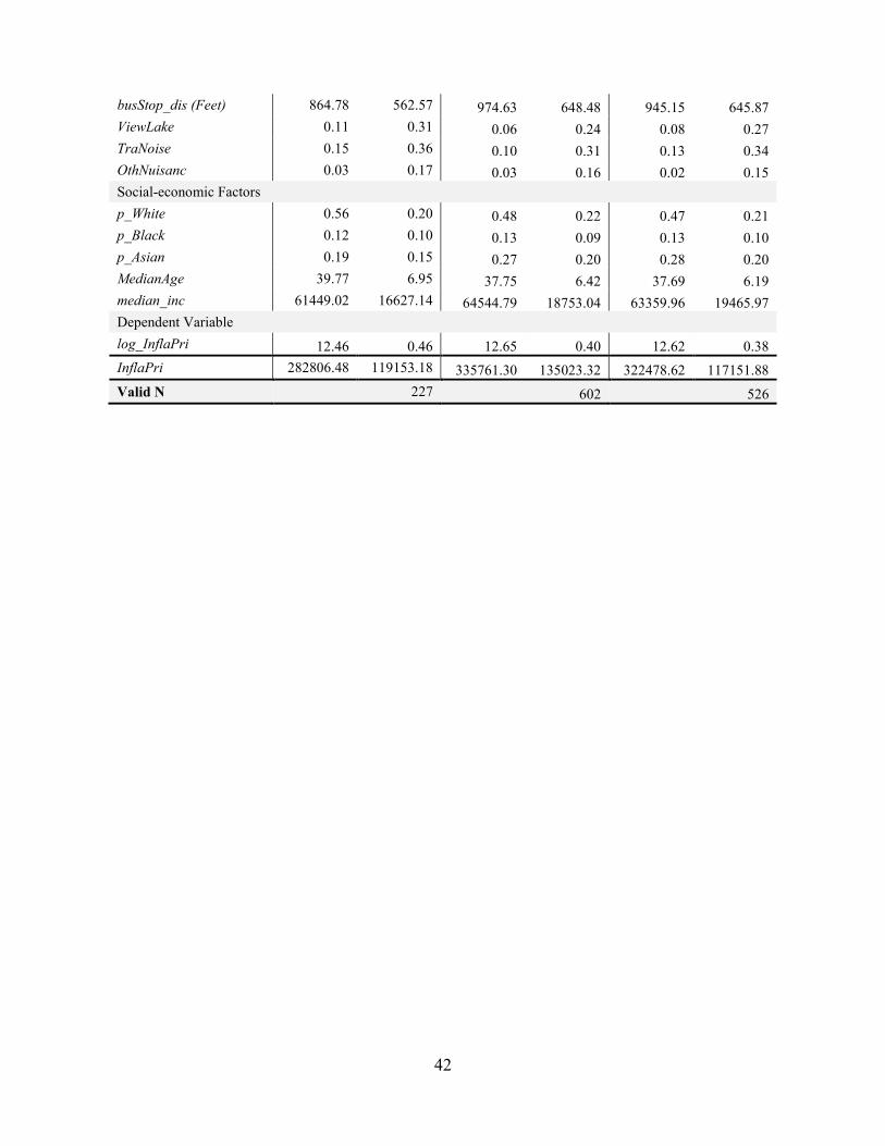
42
busStop_dis (Feet) 864.78 562.57 974.63 648.48 945.15 645.87
ViewLake 0.11 0.31 0.06 0.24 0.08 0.27
TraNoise 0.15 0.36 0.10 0.31 0.13 0.34
OthNuisanc 0.03 0.17 0.03 0.16 0.02 0.15
Social-economic Factors
p_White 0.56 0.20 0.48 0.22 0.47 0.21
p_Black 0.12 0.10 0.13 0.09 0.13 0.10
p_Asian 0.19 0.15 0.27 0.20 0.28 0.20
MedianAge 39.77 6.95 37.75 6.42 37.69 6.19
median_inc 61449.02 16627.14 64544.79 18753.04 63359.96 19465.97
Dependent Variable
log_InflaPri 12.46 0.46 12.65 0.40 12.62 0.38
InflaPri 282806.48 119153.18 335761.30 135023.32 322478.62 117151.88
Valid N 227 602 526
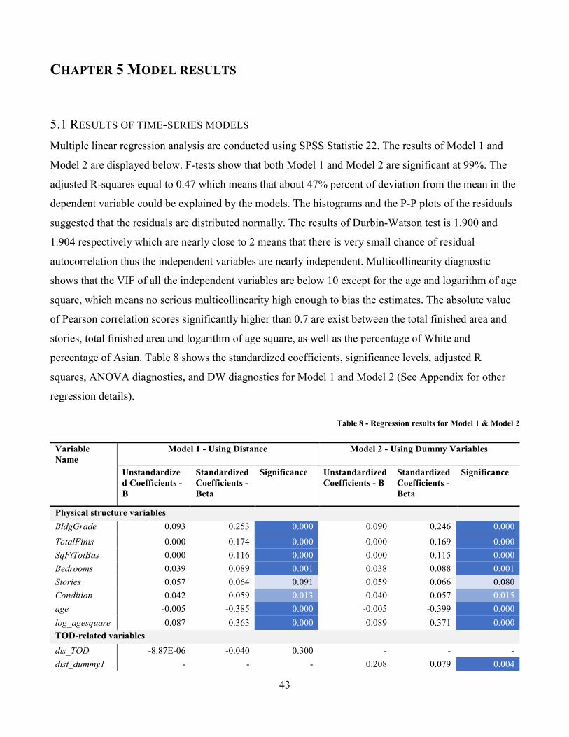
43
CHAPTER 5 MODEL RESULTS
5.1 RESULTS OF TIME-SERIES MODELS
Multiple linear regression analysis are conducted using SPSS Statistic 22. The results of Model 1 and
Model 2 are displayed below. F-tests show that both Model 1 and Model 2 are significant at 99%. The
adjusted R-squares equal to 0.47 which means that about 47% percent of deviation from the mean in the
dependent variable could be explained by the models. The histograms and the P-P plots of the residuals
suggested that the residuals are distributed normally. The results of Durbin-Watson test is 1.900 and
1.904 respectively which are nearly close to 2 means that there is very small chance of residual
autocorrelation thus the independent variables are nearly independent. Multicollinearity diagnostic
shows that the VIF of all the independent variables are below 10 except for the age and logarithm of age
square, which means no serious multicollinearity high enough to bias the estimates. The absolute value
of Pearson correlation scores significantly higher than 0.7 are exist between the total finished area and
stories, total finished area and logarithm of age square, as well as the percentage of White and
percentage of Asian. Table 8 shows the standardized coefficients, significance levels, adjusted R
squares, ANOVA diagnostics, and DW diagnostics for Model 1 and Model 2 (See Appendix for other
regression details).
Table 8 - Regression results for Model 1 & Model 2
Variable
Name
Model 1 - Using Distance Model 2 - Using Dummy Variables
Unstandardize
d Coefficients -
B
Standardized
Coefficients -
Beta
Significance Unstandardized
Coefficients - B
Standardized
Coefficients -
Beta
Significance
Physical structure variables
BldgGrade 0.093 0.253 0.000 0.090 0.246 0.000
TotalFinis 0.000 0.174 0.000 0.000 0.169 0.000
SqFtTotBas 0.000 0.116 0.000 0.000 0.115 0.000
Bedrooms 0.039 0.089 0.001 0.038 0.088 0.001
Stories 0.057 0.064 0.091 0.059 0.066 0.080
Condition 0.042 0.059 0.013 0.040 0.057 0.015
age -0.005 -0.385 0.000 -0.005 -0.399 0.000
log_agesquare 0.087 0.363 0.000 0.089 0.371 0.000
TOD-related variables
dis_TOD -8.87E-06 -0.040 0.300 - - -
dist_dummy1 - - - 0.208 0.079 0.004
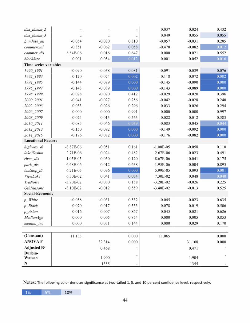
44
dist_dummy2 - - - 0.037 0.024 0.432
dist_dummy3 - - - 0.049 0.055 0.055
Landuse_mi -0.054 -0.030 0.310 -0.057 -0.031 0.285
commercial -0.351 -0.062 0.058 -0.470 -0.082 0.012
commer_dis 8.84E-06 0.016 0.647 0.000 0.021 0.552
blockSize 0.001 0.054 0.012 0.001 0.052 0.016
Time-series variables
1990_1991 -0.090 -0.038 0.081 -0.091 -0.039 0.076
1992_1993 -0.120 -0.074 0.002 -0.118 -0.072 0.002
1994_1995 -0.144 -0.089 0.000 -0.145 -0.090 0.000
1996_1997 -0.143 -0.089 0.000 -0.143 -0.089 0.000
1998_1999 -0.028 -0.020 0.412 -0.029 -0.020 0.396
2000_2001 -0.041 -0.027 0.256 -0.042 -0.028 0.240
2002_2003 0.033 0.026 0.296 0.033 0.026 0.294
2006_2007 0.000 0.000 0.991 0.000 0.000 0.997
2008_2009 -0.024 -0.013 0.563 -0.022 -0.012 0.583
2010_2011 -0.085 -0.046 0.039 -0.083 -0.045 0.044
2012_2013 -0.150 -0.092 0.000 -0.149 -0.092 0.000
2014_2015 -0.176 -0.082 0.000 -0.176 -0.082 0.000
Locational Factors
highway_di -8.87E-06 -0.051 0.161 -1.00E-05 -0.058 0.110
lakeWashin 2.71E-06 0.024 0.482 2.67E-06 0.023 0.491
river_dis -1.05E-05 -0.050 0.120 -8.67E-06 -0.041 0.175
park_dis -6.68E-06 -0.012 0.638 -1.95E-06 -0.004 0.893
busStop_di 6.21E-05 0.096 0.000 5.99E-05 0.093 0.001
ViewLake 6.30E-02 0.041 0.074 7.30E-02 0.048 0.040
TraNoise -3.70E-02 -0.030 0.158 -3.20E-02 -0.026 0.225
OthNuisanc -3.10E-02 -0.012 0.559 -3.40E-02 -0.013 0.525
Social-Economic
p_White -0.058 -0.031 0.532 -0.045 -0.023 0.635
p_Black 0.070 0.017 0.553 0.078 0.019 0.506
p_Asian 0.016 0.007 0.867 0.045 0.021 0.626
MedianAge 0.000 0.005 0.854 0.000 0.005 0.853
median_inc 0.000 0.031 0.144 0.000 0.029 0.170
(Constant) 11.133 0.000 11.065 0.000
ANOVA F 32.314 0.000 31.108 0.000
Adjusted R2 0.468 - 0.471 -
Durbin-
Watson 1.900 -
1.904 -
N 1355 - 1355 -
Notes: The following color denotes significance at two-tailed 1, 5, and 10 percent confidence level, respectively.
1% 5% 10%
45
Since the dependent variable, the inflated property value, is measured in logarithmic term, coefficients
are interpreted as the percentage change of Y driven by a unit change of X. For unstandardized variable
X, a unit means the original unscaled unit, for example, a unit increase for total finished area is a square
footage increase. However, the different scales of units of independent variables make it difficult to
assess the relative importance of each variables, therefore standardized coefficients are used which
removes the problem of comparing variables with different units by standardizing each variables before
doing the regression analysis. For standardized variable X, a unit increase in the standardized variables
is equivalent to a standard deviation (SD) increase in the unstandardized variables. Typically, scaled
variables with larger standardized coefficients have larger effects on the dependent variable. From the
results, scaled variables with significant standardized coefficients larger than 0.1 are building grade,
total finish area above the floor, square footage of basement, age and logarithm of age square, indicating
that the physical structure of the building is the most important determinant of housing price. However it
makes little sense to standardize dummy variables because dummy variables cannot be increased by a
standard deviation, therefore regular interpretation for standardized coefficients does not apply. SPSS
software uses “B” for unstandardized coefficients, and “Beta” for standardized coefficients. Thus, this
chapter will interpret standardized“Beta” coefficients for scaled independent variable, and
unstandardized “B” coefficients for dummy variables.
Physical Structure
Most physical structure variables show high significance. The building grade, total finished area, square
footage of total basement, and number of bedrooms have the expected positive signs and significant at
99% level of confidence. For instance, the willingness to pay for a SD increment of total finished area
(about 746 square feet or 69 square meters) is around 17%, which means that a 100 square feet increase
of housing size would increase the housing value for about 2.3%. The willingness to pay for a SD
increment of total basement (about 546 square footage) is around 12%, means that a 100 square footage
(around 9.3 square meter) increase of basement would increase the property value for about 2.2%. Add a
bedroom would probably increase the housing price for about 8.8%, and add a grade of the house (e.g.
from low to fair) would rise up the housing price for about 25%. Both age and logarithm of age square
are significant at 99% level of confidence. The age of building has an expected negative relationship to
the property, e.g., a 30-year-elder house has a 38% to 39% lower housing value than a new house when
46
all else being equal. But this does not mean older houses are always cheaper than newer houses. When
looking at logarithm of age square, the coefficient is significantly positive, indicating that the
relationship between age and housing price is not linear. Some extremely old house may be more
expensive than a current new house. The coefficients of building condition and the building story are
significantly positive at 95% and 90% level of confidence respectively in the models, and indicate a 5%-
6% rise in the property value with each 0.5-level increase in the building condition, or a 0.5-stories
increase for the building.
Locational Factors
Among locational factors, only the distance to bus stops and view of Lake Washington are significant
and positively relate with property value at both Model 1 and Model 2. The estimates of the semi-
logarithmic function imply that increase the distance between property and bus stop for a standard
deviation, that is 634 feet (around 200 meters) is associated with a property value increase of about
9.3 % - 9.6%. Houses with Lake Washington view is worth 6.3% to 7.3% more than those without lake
view. Other locational variables are not significant at both Model 1 and Model 2. Thus, hypotheses
concerning proximity to highways decreases housing value and proximity to parks increases housing
value are not validated in this study.
Social-economic Factors
No significant relationship are found between social-economic factors and housing price. This is likely
due, in part, to the insufficient block and block-group sample size for the social-economic data and, in
part, to the highly correlation between independent variables of percentage of White and percentage of
Asian, with a Pearson Correlation for about 0.8 at two-tailed 0.01 level (See Appendix for correlation
diagnosis detail).
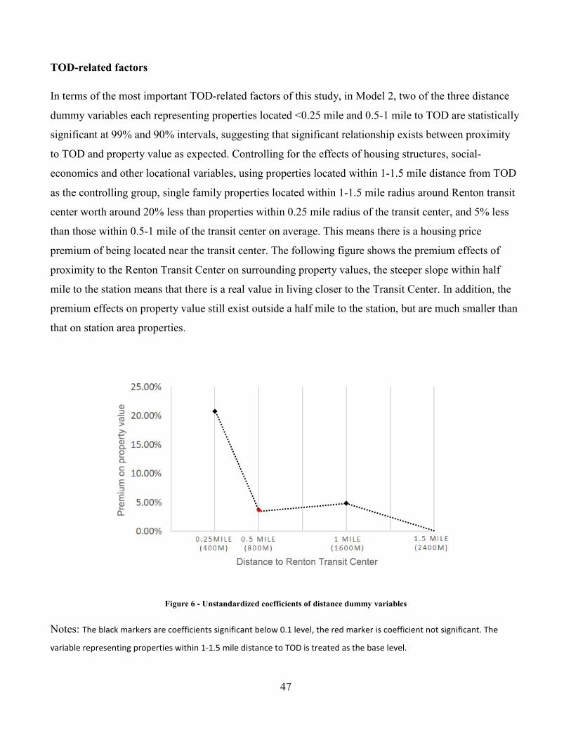
47
TOD-related factors
In terms of the most important TOD-related factors of this study, in Model 2, two of the three distance
dummy variables each representing properties located <0.25 mile and 0.5-1 mile to TOD are statistically
significant at 99% and 90% intervals, suggesting that significant relationship exists between proximity
to TOD and property value as expected. Controlling for the effects of housing structures, social-
economics and other locational variables, using properties located within 1-1.5 mile distance from TOD
as the controlling group, single family properties located within 1-1.5 mile radius around Renton transit
center worth around 20% less than properties within 0.25 mile radius of the transit center, and 5% less
than those within 0.5-1 mile of the transit center on average. This means there is a housing price
premium of being located near the transit center. The following figure shows the premium effects of
proximity to the Renton Transit Center on surrounding property values, the steeper slope within half
mile to the station means that there is a real value in living closer to the Transit Center. In addition, the
premium effects on property value still exist outside a half mile to the station, but are much smaller than
that on station area properties.
Figure 6 - Unstandardized coefficients of distance dummy variables
Notes: The black markers are coefficients significant below 0.1 level, the red marker is coefficient not significant. The
variable representing properties within 1-1.5 mile distance to TOD is treated as the base level.
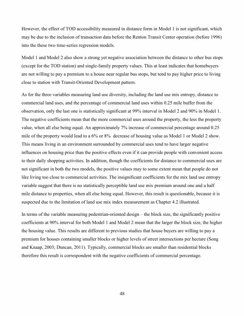
48
However, the effect of TOD accessibility measured in distance form in Model 1 is not significant, which
may be due to the inclusion of transaction data before the Renton Transit Center operation (before 1996)
into the these two time-series regression models.
Model 1 and Model 2 also show a strong yet negative association between the distance to other bus stops
(except for the TOD station) and single-family property values. This at least indicates that homebuyers
are not willing to pay a premium to a house near regular bus stops, but tend to pay higher price to living
close to station with Transit-Oriented Development pattern.
As for the three variables measuring land use diversity, including the land use mix entropy, distance to
commercial land uses, and the percentage of commercial land uses within 0.25 mile buffer from the
observation, only the last one is statistically significant at 99% interval in Model 2 and 90% in Model 1.
The negative coefficients mean that the more commercial uses around the property, the less the property
value, when all else being equal. An approximately 7% increase of commercial percentage around 0.25
mile of the property would lead to a 6% or 8% decrease of housing value as Model 1 or Model 2 show.
This means living in an environment surrounded by commercial uses tend to have larger negative
influences on housing price than the positive effects even if it can provide people with convenient access
to their daily shopping activities. In addition, though the coefficients for distance to commercial uses are
not significant in both the two models, the positive values may to some extent mean that people do not
like living too close to commercial activities. The insignificant coefficients for the mix land use entropy
variable suggest that there is no statistically perceptible land use mix premium around one and a half
mile distance to properties, when all else being equal. However, this result is questionable, because it is
suspected due to the limitation of land use mix index measurement as Chapter 4.2 illustrated.
In terms of the variable measuring pedestrian-oriented design – the block size, the significantly positive
coefficients at 90% interval for both Model 1 and Model 2 mean that the larger the block size, the higher
the housing value. This results are different to previous studies that house buyers are willing to pay a
premium for houses containing smaller blocks or higher levels of street intersections per hectare (Song
and Knaap, 2003; Duncan, 2011). Typically, commercial blocks are smaller than residential blocks
therefore this result is correspondent with the negative coefficients of commercial percentage.
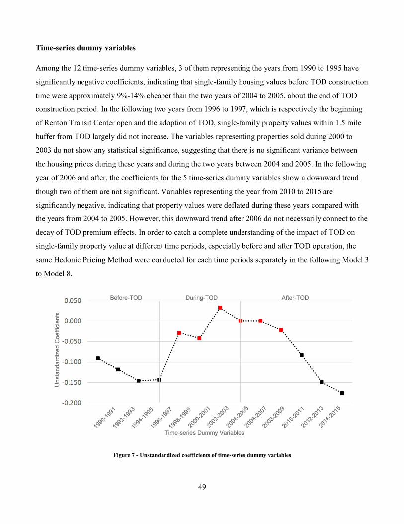
49
Time-series dummy variables
Among the 12 time-series dummy variables, 3 of them representing the years from 1990 to 1995 have
significantly negative coefficients, indicating that single-family housing values before TOD construction
time were approximately 9%-14% cheaper than the two years of 2004 to 2005, about the end of TOD
construction period. In the following two years from 1996 to 1997, which is respectively the beginning
of Renton Transit Center open and the adoption of TOD, single-family property values within 1.5 mile
buffer from TOD largely did not increase. The variables representing properties sold during 2000 to
2003 do not show any statistical significance, suggesting that there is no significant variance between
the housing prices during these years and during the two years between 2004 and 2005. In the following
year of 2006 and after, the coefficients for the 5 time-series dummy variables show a downward trend
though two of them are not significant. Variables representing the year from 2010 to 2015 are
significantly negative, indicating that property values were deflated during these years compared with
the years from 2004 to 2005. However, this downward trend after 2006 do not necessarily connect to the
decay of TOD premium effects. In order to catch a complete understanding of the impact of TOD on
single-family property value at different time periods, especially before and after TOD operation, the
same Hedonic Pricing Method were conducted for each time periods separately in the following Model 3
to Model 8.
Figure 7 - Unstandardized coefficients of time-series dummy variables
50
Notes: The black markers are coefficients significant below 0.1 level, the red markers are coefficients not significant. The
variable representing properties sold during 2004 to 2005 is treated as the base level.
5.2 RESULTS OF BEFORE-DURING-AFTER MODELS
Overall, F-tests show Model 3, 4, and 5 are significant at 99%. The adjusted R-squares of these three
models equal to 0.37, 0.51 and 0.47, respectively. The results of histograms and p-p plots of residuals,
DW tests and Collinearity diagnostics are acceptable. The absolute value of Pearson correlation scores
significantly higher than 0.7 are exist between the total finished area and building grade, total finished
area and stories, and between the percentage of White and percentage of Asian in Model 4 and Model 5.
Table 9 - Regression results for Model 3, 4 and 5
Variable
Name
Model 3 - Pre TOD Model 4 - During TOD Model 5 - Post TOD
Unstandar
dized-B
Standa
rdized-
Beta
Sig. Unstandar
dized-B
Standa
rdized-
Beta
Sig. Unstandar
dized-B
Standa
rdized-
Beta
Sig.
Physical structure variables
BldgGrade 0.126 0.298 0.011 0.101 0.283 0.000 0.052 0.152 0.015
TotalFinis -3.65E-05 -0.051 0.571 0.000 0.254 0.000 0.000 0.306 0.000
SqFtTotBas 0.000 0.168 0.025 0.000 0.154 0.000 0.000 0.119 0.009
Bedrooms 0.038 0.078 0.305 0.025 0.056 0.157 0.044 0.109 0.015
Stories 0.211 0.164 0.052 0.072 0.082 0.136 0.034 0.042 0.522
Condition 0.025 0.032 0.610 0.029 0.039 0.289 0.057 0.091 0.015
age -0.02 -1.145 0.000 -0.006 -0.478 0.000 -0.003 -0.231 0.071
log_agesquare 0.513 1.149 0.000 0.108 0.444 0.002 0.049 0.242 0.064
TOD-related variables
dis_TOD 3.61E-05 0.152 0.170 -2.38E-05 -0.112 0.068 -2.74E-05 -0.129 0.030
Landuse_mi 0.316 0.142 0.109 -0.145 -0.083 0.057 -0.034 -0.020 0.672
commercial -0.627 -0.094 0.374 -0.292 -0.050 0.299 -0.545 -0.109 0.035
commer_dis -1.83E-05 -0.029 0.770 3.71E-05 0.067 0.190 -1.85E-06 -0.004 0.948
blockSize 0.002 0.081 0.248 0.001 0.046 0.142 0.001 0.074 0.039
Locational factors
highway_dis -1.24E-05 -0.066 0.557 -9.16E-06 -0.053 0.324 -8.34E-06 -0.052 0.365
lake_dis -1.02E-05 -0.080 0.395 1.79E-06 0.016 0.751 1.01E-05 0.094 0.084
river_dis -1.24E-05 -0.052 0.568 -1.98E-05 -0.097 0.046 1.10E-05 0.056 0.293
park_dis -8.60E-06 -0.014 0.843 -2.16E-05 -0.040 0.304 1.58E-05 0.031 0.467
busStop_dis 2.92E-05 0.036 0.639 4.38E-05 0.070 0.091 7.95E-05 0.136 0.003
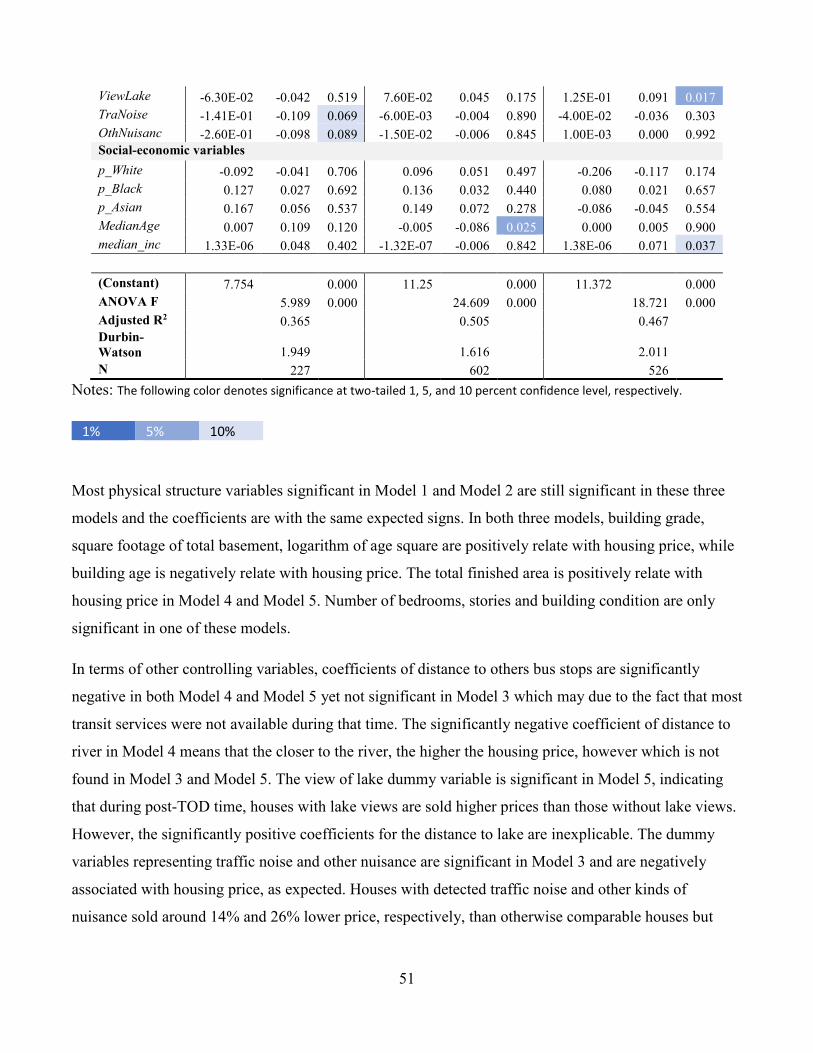
51
ViewLake -6.30E-02 -0.042 0.519 7.60E-02 0.045 0.175 1.25E-01 0.091 0.017
TraNoise -1.41E-01 -0.109 0.069 -6.00E-03 -0.004 0.890 -4.00E-02 -0.036 0.303
OthNuisanc -2.60E-01 -0.098 0.089 -1.50E-02 -0.006 0.845 1.00E-03 0.000 0.992
Social-economic variables
p_White -0.092 -0.041 0.706 0.096 0.051 0.497 -0.206 -0.117 0.174
p_Black 0.127 0.027 0.692 0.136 0.032 0.440 0.080 0.021 0.657
p_Asian 0.167 0.056 0.537 0.149 0.072 0.278 -0.086 -0.045 0.554
MedianAge 0.007 0.109 0.120 -0.005 -0.086 0.025 0.000 0.005 0.900
median_inc 1.33E-06 0.048 0.402 -1.32E-07 -0.006 0.842 1.38E-06 0.071 0.037
(Constant) 7.754 0.000 11.25 0.000 11.372 0.000
ANOVA F 5.989 0.000 24.609 0.000 18.721 0.000
Adjusted R2 0.365 0.505 0.467
Durbin-
Watson 1.949 1.616 2.011
N 227 602 526
Notes: The following color denotes significance at two-tailed 1, 5, and 10 percent confidence level, respectively.
1% 5% 10%
Most physical structure variables significant in Model 1 and Model 2 are still significant in these three
models and the coefficients are with the same expected signs. In both three models, building grade,
square footage of total basement, logarithm of age square are positively relate with housing price, while
building age is negatively relate with housing price. The total finished area is positively relate with
housing price in Model 4 and Model 5. Number of bedrooms, stories and building condition are only
significant in one of these models.
In terms of other controlling variables, coefficients of distance to others bus stops are significantly
negative in both Model 4 and Model 5 yet not significant in Model 3 which may due to the fact that most
transit services were not available during that time. The significantly negative coefficient of distance to
river in Model 4 means that the closer to the river, the higher the housing price, however which is not
found in Model 3 and Model 5. The view of lake dummy variable is significant in Model 5, indicating
that during post-TOD time, houses with lake views are sold higher prices than those without lake views.
However, the significantly positive coefficients for the distance to lake are inexplicable. The dummy
variables representing traffic noise and other nuisance are significant in Model 3 and are negatively
associated with housing price, as expected. Houses with detected traffic noise and other kinds of
nuisance sold around 14% and 26% lower price, respectively, than otherwise comparable houses but
52
without these nuisance. However, these effects have not found to be significant in during and post TOD
periods.
Homeowner median income is positively relate to single-family property value and the coefficients are
significant at 95% confidence level in Model 5. This somewhat validates the hypothesis that people tend
to live in a place where residents have the similar income as theirs.
Finally, we turn to TOD-related factors, the focus of this study. None of them are tested to be significant
in pre-TOD time. The hypothesis concerning proximity to transit center increases property value is to
some extent validated in this before-during-after analysis. In Model 3, the coefficient of the variable
measuring distance to TOD is insignificant and positive, indicating there is no accessibility premium
during pre-TOD time. However, the accessibility effect, on the contrary, is significant after TOD took
into effect and still maintains in post-TOD time. In TOD-construction time, increase in the accessibility
to the Transit Center by one standard deviation distance (1890 feet, or about 0.36 mile) is associated
with an 11% increase of the housing price. In post-TOD time, the premium effect of transit accessibility
seems even stronger, because increase in the accessibility by one standard deviation distance (1781 feet,
or about 0.33 mile) is linked to a 13% increase of the housing price.
The variables representing land use mix entropy and commercial percentage are significantly negative in
TOD construction time and post-TOD time respectively, which to some extent indicating that people
still do not like living surrounded by too much non-residential commercial activities. The positive
coefficients of block size in Model 5 indicate that houses tend to have lower values if locate in smaller
blocks, which corresponds to the results of commercial percentage since commercial district typically
has smaller block size. Curiously, these negative effects of commercial tend to be significant after TOD
operation, which may suggest that TOD construction or commercial activities create some negative
influences on surrounding housing price as previous studies found. But this is also suspected due to the
limitation of using the current land use data for measuring previous year condition.
The following are the regression results for Model 6 to Model 8 using three distance dummy variables to
measure transit accessibility. The overall statistical results are similar to Model 3 to Model 5.
Table 10 - Regression results for Model 6, 7 and 8
Variable
Name
Model 6 - Pre TOD Model 7 - During TOD Model 8 - Post TOD
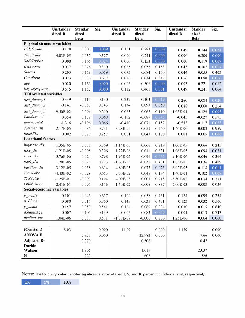
53
Unstandar
dized-B
Standar
dized-
Beta
Sig. Unstandar
dized-B
Standar
dized-
Beta
Sig. Unstandar
dized-B
Standar
dized-
Beta
Sig.
Physical structure variables
BldgGrade 0.128 0.302 0.009 0.101 0.283 0.000 0.049 0.144 0.021
TotalFinis -4.03E-05 -0.057 0.527 0.000 0.244 0.000 0.000 0.300 0.000
SqFtTotBas 0.000 0.165 0.024 0.000 0.153 0.000 0.000 0.119 0.008
Bedrooms 0.037 0.076 0.310 0.025 0.056 0.153 0.043 0.107 0.017
Stories 0.203 0.158 0.059 0.073 0.084 0.130 0.044 0.055 0.403
Condition 0.023 0.030 0.627 0.026 0.034 0.347 0.056 0.090 0.016
age -0.020 -1.161 0.000 -0.006 -0.508 0.000 -0.003 -0.221 0.082
log_agesquare 0.515 1.152 0.000 0.112 0.461 0.001 0.049 0.241 0.064
TOD-related variables
dist_dummy1 0.349 0.111 0.130 0.232 0.103 0.019 0.260 0.084 0.029 dist_dummy2 -0.141 -0.081 0.343 0.134 0.093 0.050 0.088 0.060 0.214
dist_dummy3 -9.50E-02 -0.096 0.210 0.063 0.067 0.110 1.05E-01 0.129 0.005
Landuse_mi 0.354 0.159 0.068 -0.152 -0.087 0.045 -0.045 -0.027 0.575
commercial -1.316 -0.196 0.066 -0.410 -0.071 0.157 -0.583 -0.117 0.023
commer_dis -2.17E-05 -0.035 0.731 3.28E-05 0.059 0.240 1.46E-06 0.003 0.959
blockSize 0.002 0.079 0.257 0.001 0.043 0.170 0.001 0.065 0.068
Locational factors
highway_dis -1.35E-05 -0.071 0.509 -1.14E-05 -0.066 0.219 -1.06E-05 -0.066 0.245
lake_dis -1.21E-05 -0.095 0.306 1.22E-06 0.011 0.831 1.06E-05 0.098 0.071
river_dis -5.76E-06 -0.024 0.768 -1.96E-05 -0.096 0.035 9.10E-06 0.046 0.364
park_dis 1.28E-05 0.021 0.773 -1.68E-05 -0.031 0.431 1.83E-05 0.036 0.409
busStop_dis 3.12E-05 0.038 0.614 4.80E-05 0.077 0.073 6.92E-05 0.118 0.011
ViewLake -4.40E-02 -0.029 0.653 7.50E-02 0.045 0.184 1.40E-01 0.102 0.008
TraNoise -1.25E-01 -0.097 0.104 4.00E-03 0.003 0.918 -3.80E-02 -0.034 0.331
OthNuisanc -2.41E-01 -0.091 0.116 -1.60E-02 -0.006 0.837 7.00E-03 0.003 0.936
Social-economic variables
p_White -0.101 -0.045 0.677 0.104 0.056 0.461 -0.174 -0.099 0.254
p_Black 0.080 0.017 0.800 0.148 0.035 0.401 0.123 0.032 0.500
p_Asian 0.157 0.053 0.561 0.164 0.080 0.234 -0.030 -0.015 0.840
MedianAge 0.007 0.101 0.139 -0.005 -0.083 0.029 0.001 0.013 0.743
median_inc 1.04E-06 0.037 0.511 -1.38E-07 -0.006 0.836 1.25E-06 0.064 0.060
(Constant) 8.03 0.000 11.09 0.000 11.159 0.000
ANOVA F 5.921 0.000 22.982 0.000 17.66 0.000
Adjusted R2 0.379 0.506 0.47
Durbin-
Watson 1.965 1.615 2.037
N 227 602 526
Notes: The following color denotes significance at two-tailed 1, 5, and 10 percent confidence level, respectively.
1% 5% 10%
54
In terms of the three dummy variables measuring distance to TOD, for Model 6 (the post-TOD period),
none of the three distance dummy variables is statistically significant. Only the coefficient for the first
one which capturing properties located within 0.25 mile is positive, the other two dummy variables are
negatively related with housing price. One plausible hypothesis is that the first distance dummy variable
would probably capture the effect of other amenities (e.g. a public theater or something else) before
TOD construction in that area on surrounding housing price, or the premium effect of TOD on station
area properties was likely happened as early as the decision making stage but had not widely affected
property values outside a quarter mile distance. These positive impacts had probably made houses
located within 0.25 mile in approximately 34.9% more expensive than houses located within 1-1.5 mile,
but the positive influence dissipate quickly outside 0.25 mile range.
However, for Model 7 (TOD construction period), the coefficients for all the three distance dummy
variables are positive, and two of them are significant at either 95% or 90% intervals, indicating that a
housing price premium took place during the implementation of TOD. Coefficients of the two
significant distance dummy variables can be interpreted as houses located within 0.25 mile and 0.25-0.5
mile to TOD were 23.2% and 13.4% higher in price, compared with the houses located 1-1.5 mile
distance to TOD. During post-TOD period, the three distance dummy variables are still positive, and
there are still two distance dummy variables significant at 95% intervals. Results show that houses
within 0.25 mile and 0.5-1 mile of TOD were 26% and 10.5% higher in price compared with houses
located 1-1.5 mile distance to TOD during post-TOD construction time.
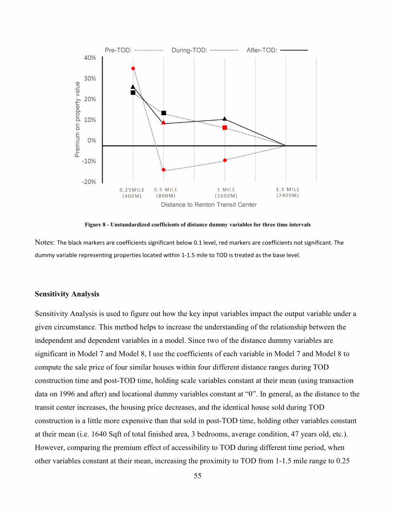
55
Figure 8 - Unstandardized coefficients of distance dummy variables for three time intervals
Notes: The black markers are coefficients significant below 0.1 level, red markers are coefficients not significant. The
dummy variable representing properties located within 1-1.5 mile to TOD is treated as the base level.
Sensitivity Analysis
Sensitivity Analysis is used to figure out how the key input variables impact the output variable under a
given circumstance. This method helps to increase the understanding of the relationship between the
independent and dependent variables in a model. Since two of the distance dummy variables are
significant in Model 7 and Model 8, I use the coefficients of each variable in Model 7 and Model 8 to
compute the sale price of four similar houses within four different distance ranges during TOD
construction time and post-TOD time, holding scale variables constant at their mean (using transaction
data on 1996 and after) and locational dummy variables constant at “0”. In general, as the distance to the
transit center increases, the housing price decreases, and the identical house sold during TOD
construction is a little more expensive than that sold in post-TOD time, holding other variables constant
at their mean (i.e. 1640 Sqft of total finished area, 3 bedrooms, average condition, 47 years old, etc.).
However, comparing the premium effect of accessibility to TOD during different time period, when
other variables constant at their mean, increasing the proximity to TOD from 1-1.5 mile range to 0.25
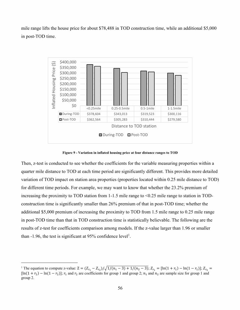
56
mile range lifts the house price for about $78,488 in TOD construction time, while an additional $5,000
in post-TOD time.
Figure 9 - Variation in inflated housing price at four distance ranges to TOD
Then, z-test is conducted to see whether the coefficients for the variable measuring properties within a
quarter mile distance to TOD at each time period are significantly different. This provides more detailed
variation of TOD impact on station area properties (properties located within 0.25 mile distance to TOD)
for different time periods. For example, we may want to know that whether the 23.2% premium of
increasing the proximity to TOD station from 1-1.5 mile range to <0.25 mile range to station in TOD-
construction time is significantly smaller than 26% premium of that in post-TOD time; whether the
additional $5,000 premium of increasing the proximity to TOD from 1.5 mile range to 0.25 mile range
in post-TOD time than that in TOD construction time is statistically believable. The following are the
results of z-test for coefficients comparison among models. If the z-value larger than 1.96 or smaller
than -1.96, the test is significant at 95% confidence level1.
1 The equation to compute z-value: Z = (:;< − :;=)/>1/(0� − 3) + 1/(0! − 3); :;< = [ln(1 + 3�) − ln(1 − 3�)]; :;= =[ln(1 + 3!) − ln(1 − 3!)]; 3� and 3! are coefficients for group 1 and group 2; 0� and 0! are sample size for group 1 and group 2.
<0.25mile 0.25-0.5mile 0.5-1mile 1-1.5mile
During-TOD $378,604 $343,013 $319,523 $300,116
Post-TOD $362,564 $305,283 $310,444 $279,580
$0
$50,000
$100,000
$150,000
$200,000
$250,000
$300,000
$350,000
$400,000
Infl
ate
d H
ou
sin
g P
rice
($
)
Distance to TOD station
During-TOD Post-TOD
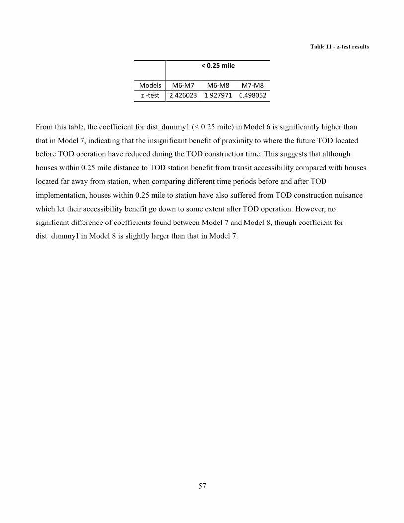
57
Table 11 - z-test results
< 0.25 mile
Models M6-M7 M6-M8 M7-M8
z -test 2.426023 1.927971 0.498052
From this table, the coefficient for dist_dummy1 (< 0.25 mile) in Model 6 is significantly higher than
that in Model 7, indicating that the insignificant benefit of proximity to where the future TOD located
before TOD operation have reduced during the TOD construction time. This suggests that although
houses within 0.25 mile distance to TOD station benefit from transit accessibility compared with houses
located far away from station, when comparing different time periods before and after TOD
implementation, houses within 0.25 mile to station have also suffered from TOD construction nuisance
which let their accessibility benefit go down to some extent after TOD operation. However, no
significant difference of coefficients found between Model 7 and Model 8, though coefficient for
dist_dummy1 in Model 8 is slightly larger than that in Model 7.
58
CHAPTER 6 CONCLUSION
In this thesis, I use the Hedonic Regression Analysis to measure the impact of Transit-Oriented
Development on single-family property value within 1.5 mile radius around Renton Transit Center, a
TOD project implemented 18 years ago in King County, WA. A series of regression models were built,
Model 1 and 2 are time-series models measuring accessibility to TOD station in different methods (one
uses distance, the other uses series of distance dummy variables), and Model 3 to Model 8 takes
longitudinal approach by dividing the housing transaction time into three periods: pre-TOD, during TOD
construction, and post-TOD intervals. Model 3 to Model 5 uses distance as a measurement of proximity
to TOD, while Model 6 to Model 8 uses distance dummy variables. Overall, the results show the dual
nature of TOD: proximity to TOD station has been capitalized into property value; however, this benefit
has also reduced more or less due to TOD-related nuisance like too much commercial around property,
or construction noise for properties located within a quarter mile distance to TOD.
Results of this study show that access to TOD transit station is not statistically significant in Model 1
measuring station accessibility by distance. This may on the one hand due to the inclusion of properties
sold before TOD operation into the database, on the other hand because that the relationship between
station proximity and housing price is not as simple as a linear function, different price effects happen
within different spatial extents and during different time periods. However, when using three dummy
variables to represent four ranges of distance to TOD stations, all the dummy variables are positive and
two of them are statistically significant, indicating that in general proximity to Renton Transit Center
have positively influenced the prices of surrounding homes. In contrast, a notable result is that the
coefficients for the variable representing distance to other bus stops are significantly positive, suggesting
that the smaller distance to other bus stops, the lower housing price. This may indicate that stations with
TOD pattern are at least better than normal transit stops.
When it comes to TOD, most previous studies estimated the property value impacts of transit
accessibility, and only very few estimated other TOD components like mixed land use and walkable
pedestrian design. This thesis fills this gap by estimating the impact of land use mix entropy, percentage
of commercial land use, distance to nearest commercial uses, and block size on property values. Results
from the models illustrate that the higher percentage of commercial around 0.25 mile of the property, or
the smaller the block size, the lower market value for that property. This means though TOD typically
59
entails mixed land use and walkable pedestrian design which enhances convenience to various kind of
retail and commercial services, the negative aspects such as traffic noise and migrants impede the
willingness to pay for houses located in an area with too much commercial around it, or with too dense
street network systems. Thus, future research should try to find an appropriate mixed development
strategy for TOD.
This thesis also uses the real estate transaction data over a 26-year period, the first two models take time-
series approaches by dividing the 26-year into 13 time periods using 12 time dummy variables.
Controlling for the effect of other variables including large economic background, results found that
properties sold before TOD operation and the two years of the beginning of TOD (1996-1997) are
significantly less expensive than properties sold during 2004-2005, in TOD operation time. Properties
sole after 2009 are also less expensive than those sold during 2004-2005. Moreover, no significant
difference found between the properties sold during 1998 to 2009 and properties sold in 2004-2005.
Results from longitudinal models reveal that before the implementation of TOD, proximity to TOD
station has insignificant positive effects for houses within 0.25 miles. This positive influences on
property value are probably due to presence of other amenities around the station before TOD
implementation or the premium effect of TOD began as early as the decision making stage. However, all
the distance to TOD dummy variables are positive and gradually decreasing in TOD construction time
and in post-TOD time, and two of them are significant in each of these time periods, suggesting that
accessibility to transit station has raised surrounding housing value after the station went into operation.
Yet when comparing the coefficients of the variable representing station area properties (properties
located within 0.25 mile distance to TOD) during different time periods, results show that the premium
effect of accessibility to TOD on station area (i.e. within 0.25 mile) property has actually reduced after
TOD operation than before-TOD time.
While this study seeks to measure the real impact of TOD on single-family property value using time-
series models and before-during-after models controlling for the influences of other property value
factors, there are some limitations:
First, this study does not fully control the effects of other non-TOD variables. It is possible that social-
economic data and locational data (including some TOD-related variables like distance to commercial,
mixed land use and block size) used in this study are inaccurate because they are limited to current
situations but not the situation at the transaction time. All the social-economic data are from Census
60
2010 even if some of the properties were sold 10 years ago. As for locational variables, it is extremely
difficult to obtain GIS spatial data in previous years. All of these would affect the result of this study;
however, the most important key variable – distance to TOD would not be affected.
Second, this study focuses on a case of bus transit center with TOD pattern in Seattle Metropolitan Area.
Since housing price effect of TOD is likely to vary considerably by different transit types and settings as
illustrated in Chapter 2, this study may be less convincing for premium effect of other kind of transit
types in other part of region.
This study measures the impact of Transit-Oriented Development (TOD) on single family property value
using a real-world TOD project in Seattle Metropolitan Area. Major results of this study corroborate the
mainstream view that TOD have premium effects on surrounding property value, but this benefit can
also reduce due to TOD-related nuisance. In this case, local government under fiscal stress can generate
additional revenue source through innovative transit-oriented development projects and programs if it
finds an appropriate strategy for mixed land use development near the station.
61
References
John Pucher. (2004). Public Transportation. In Hanson, S., & In Giuliano, G. (2004). The geography of urban
transportation (Third Edition). New York: Guilford Press.
O'Sullivan, A. (2012). Urban economics. New York, NY: McGraw-Hill/Irwin.
Business, Transportation, and Housing Agency, & California Department of Transportation. (2002). Statewide
Transit-Oriented Development Study - Factors for Success in California.
United States Government Accountability Office. (2014). Public Transportation - Multiple Factors Influence Extent
of Transit-Oriented Development.
Cervero et al. (2004). Transit-Oriented Development in the United States: Experiences, Challenges, and Prospects.
Transportation Research Board.
Suzuki et al. (2015). Financing Transit-Oriented Development with Land Values - Adapting Land Value Capture
in Developing Countries. World Bank Group.
Thünen, J. H., & In Hall, P. (1966). Isolated state: An English edition of Der isolierte Staat. Oxford: Pergamon
Press.
William Alonso. (1964). Location and Land Use: Towards a General Theory of Land Rent. Cambridge, MA:
Harvard University Press.
Bowes, D. R., & Ihlanfeldt, K. R. (2001). Identifying the Impacts of Rail Transit Stations on Residential Property
Values. Journal of Urban Economics, 50, 1, 1-25.
Bartholomew, K., & Ewing, R. (2011). Hedonic Price Effects of Pedestrian- and Transit-Oriented
Development. Journal of Planning Literature, 26, 1, 18-34.
Ewing, R., & Cervero, R. (2010). Travel and the Built Environment. Journal of the American Planning
Association, 76, 3, 265-294.
Kahn, M. E. (2007). Gentrification Trends in New Transit-Oriented Communities: Evidence from 14 Cities That
Expanded and Built Rail Transit Systems. Real Estate Economics, 35, 2, 155-182.
Grether, D. M., & Mieszkowski, P. (1980). The effects of nonresidential land uses on the prices of adjacent housing:
Some estimates of proximity effects. Journal of Urban Economics, 8, 1, 1-15.
Li, M. M., & Brown, H. J. (1980). Micro-Neighborhood Externalities and Hedonic Housing Prices. Land
Economics, 56, 125.
McDonald and Osuji. (1995). The effect of anticipated transportation improvement on residential land values.
Regional Science and Urban Economics, 25, 3, 261–278.
Mathur, S., & Ferrell, C. (2013). Measuring the impact of sub-urban transit-oriented developments on single-family
home values. Transportation Research Part A: Policy & Practice, 42-55.
Kay, A. I., Noland, R. B., & DiPetrillo, S. (2014). Residential property valuations near transit stations with transit-
oriented development. Journal of Transport Geography, 39, 1, 131-140.
Chen, Z., & Haynes, K. E. (2015). Impact of high speed rail on housing values: an observation from the Beijing–
Shanghai line. Journal of Transport Geography, 43.
62
Yan, Delmelle, and Duncan. (2012). The impact of a new light rail system on single-family property values in
Charlotte, North Carolina. The Journal of Transport and Land Use, 5, 2, 60–67.
Cervero and Duncan. (2002). Transit’s Value-Added Effects: Light and Commuter Rail Services and Commercial
Land Values. Transportation Research Record: Journal of the Transportation Research Board, 1805, 2–
15.
Duncan, M. (2011). The impact of transit-oriented development on housing prices in San Diego, CA. Urban
Studies, 48, 1, 101-27.
Ma, Ye, and Titheridge. (2014). Capitalization Effects of Rail Transit and Bus Rapid Transit on Residential Property
Values in a Booming Economy: Evidence from Beijing. Transportation Research Record: Journal of the
Transportation Research Board, 2451, 139–148.
Wang et al. (2015). Bus stop, property price and land value tax: A multilevel hedonic analysis with quantile
calibration. Land Use Policy, 42, 381–391.
Andersson, D. E., Shyr, O. F., & Fu, J. (2010). Does high-speed rail accessibility influence residential property
prices? Hedonic estimates from southern Taiwan. Journal of Transport Geography, 48, 1, 166.
Seo, K., Golub, A., & Kuby, M. (2014). Combined impacts of highways and light rail transit on residential property
values: a spatial hedonic price model for Phoenix, Arizona. Journal of Transport Geography, 41, 1, 53-62.
Micheal Duncan. (2008). Comparing Rail Transit Capitalization Benefits for Single-Family and Condominium
Units in San Diego, California. Transportation Research Record: Journal of the Transportation Research,
2067, 120–130.
Song, Y., & Knaap, G. (2003). New urbanism and housing values: a disaggregate assessment. Journal of Urban
Economics, 54, 2, 218-238.
Rosen, S. (1974). Hedonic Prices and Implicit Markets: Product Differentiation in Pure Competition. Journal of
Political Economy, 82, 1, 34-55.
Fein and Quigley. (1970). Measuring the Value of Housing Quality. Journal of the American Statistical Association,
65(330), 532–548.
Grether and Mieszkowski. (1974). Determinants of Real Estate Values. Journal of Urban Economics, 1, 2, 127–
145.
Daniels, C. B. (1975). The influence of racial segregation on housing prices. Journal of Urban Economics, 2, 2,
105-122.
Berry, B. J. L. (1976). Ghetto Expansion and Single-Family Housing Prices: Chicago, 1968–1972. Journal of
Urban Economics, 3, 397-423.
Schafer, R. (1976). Racial discrimination in the Boston housing market. Cambridge, Mass: Dept. of City and
Regional Planning, Harvard University.
Follain, J. J., & Malpezzi, S. (1981). The flight to the suburbs: insights gained from an analysis of central-city vs
suburban housing costs. Journal of Urban Economics, 9, 3, 381-98.
63
Chambers, D. N. (1992). The racial housing price differential and racially transitional neighborhoods. Journal of
Urban Economics, 32, 2, 214-232.
King, A. T., & Mieszkowski, P. (1973). Racial Discrimination, Segregation and the Price of Housing. Journal of
Political Economy, 81, 590.
Mankiw, N. G., & Weil, D. N. (1989). The baby boom, the baby bust, and the housing market. Regional Science
and Urban Economics, 19, 2, 235-58.
Green and Hendershott. (1993). Demographic Factors and Real House Prices (The National Bureau of Economic
Research Working Paper No. 4332). Cambridge, MA.
Bailey, M. J. (1966). Effects of Race and of Other Demographic Factors on the Values of Single-Family
Homes. Land Economics, 42, 2, 215-220.
Lapham, V. (1971). Do Blacks Pay More for Housing?. Journal of Political Economy, 79, 1244-1258
Li, M. M., & Brown, H. J. (1980). Micro-Neighborhood Externalities and Hedonic Housing Prices. Land
Economics, 56, 2, 125-141.
Gyourko, Mayer, and Sinai. (2006). Superstar Cities (The National Bureau of Economic Research Working Paper
No. 12355).
Herbert, C. E., & Belsky, E. S. (2008). The Homeownership Experience of Low-Income and Minority Households:
A Review and Synthesis of the Literature. Cityscape, 10, 2, 5-59.
Bolitzer, B., & Netusil, N. R. (2000). The impact of open spaces on property values in Portland, Oregon. Journal
of Environmental Management, 59, 3, 185-193.
Troy, A., & Grove, J. M. (2008). Property values, parks, and crime: A hedonic analysis in Baltimore,
MD. Landscape and Urban Planning, 87, 3, 233-245.
Netusil, N. R. (2005). The Effect of Environmental Zoning and Amenities on Property Values. Land
Economics, 81, 2, 227-246.
Geoghegan, J. (2002). The value of open spaces in residential land use. Land Use Policy, 19, 1, 91-98.
Anderson, S., & West, S. (2007). Open space, residential property values, and spatial context. Sage Urban Studies
Abstracts, 35, 773-789.
Nicholls, S., & Crompton, J. L. (2005). The Impact of Greenways on Property Values: Evidence from Austin,
Texas. Journal of Leisure Research, 37, 321-341.
Lansford, N. H., & Jones, L. L. (1995). Recreational and Aesthetic Value of Water Using Hedonic Price
Analysis. Journal of Agricultural and Resource Economics, 20, 2, 341-355.
Cho, S.-H et al (2006). Measuring the Contribution of Water and Green Space Amenities to Housing Values: An
Application and Comparison of Spatially Weighted Hedonic Models. Journal of Agricultural and Resource
Economics, 31, 3, 485.
Brown, J. G. M., & Pollakowski, H. O. (1977). Economic Valuation of Shoreline. Review of Economics &
Statistics, 59, 272-278.
64
Allen, G. R. (1980). Relationship between Highway Noise, Noise Mitigation, and Residential Property Values.
Virginia Highway and Transportation Research Council, Charlottesville.
Langley, C. J. (1976). Adverse Impacts of the Washington Beltway on Residential Property Values. Land
Economics, 52, 54-65.
Wilhelmsson, M. (2000). The Impact of Traffic Noise on the Values of Single-family Houses. Journal of
Environmental Planning and Management, 43, 6, 799-815.
Jon P. Nelson. (1982). Highway Noise and Property Values: A Survey of Recent Evidence. Journal of Transport
Economics and Policy, 117–138.
Jason Carey. (2001). Impact of Highways on Property Values: Case Study of the Superstition Freeway Corridor.
Arizona Department of Transportation.
Palmquist, R. B., & Washington (State). (1980). Impact of highway improvements on property values in
Washington: Final report. Olympia: The Dept.
Geoghegan, J., Wainger, L. A., & Bockstael, N. E. (1997). Spatial landscape indices in a hedonic framework: an
ecological economics analysis using GIS. Ecological Economics, 23, 3, 251-264.
Mathur, S. (2008). Impact of transportation and other jurisdictional-level infrastructure and services on housing
prices. Journal of Urban Planning and Development, 134, 1, 32-41.
Lancaster, K. J. (1966). A New Approach to Consumer Theory. Journal of Political Economy, 74, 2, 132-157.
Frank, L. D., Andresen, M. A., & Schmid, T. L. (2004). Obesity relationships with community design, physical
activity, and time spent in cars. American Journal of Preventive Medicine, 27, 2, 87-96.
Frank, L. D et al. (2007). Many Pathways from Land Use to Health: Associations between Neighborhood
Walkability and Active Transportation, Body Mass Index, and Air Quality. Journal of the American
Planning Association, 72, 1, 75-8

65
APPENDIX
Appendix-A Literatures on the impact of social-economic factors on residential property Value
Social and economic Locational Physical characteristics
Martin J.
Bailey,
1966
1950 data by
census blocks in
two Chicago
southside areas
Hedonic regression
method
race, income density, university access floors, rount feet, alley logarithm of
the amount of
federal real
estate transfer
tax paid on the
transaction
*There is no indication that blacks pay
more for housing than do other people of
similar density of occupation.
Victoria
Lapham,
1971
650 observations
of housing units
sold in Dallas in
1960
Identifying differences
between white and
black in the price paid
for common
characteristics of
housing units
identical in every way.
race minute to downtown,
location (address)
square footage, age,
number of bathrooms,
number of bedrooms,
central heat, central air,
window
housing sell
price
*There is no statistically significant
difference in black-white housing costs
King and
Mieszkows
ki, 1973
over 200 rental
units in New
Haven,
Connecticut
Hedonic regression
method
race, family size,
education of the head
of the household
distance from green space, size, quality monthly rent
inclusive of
utilities
*a pure racial discrimination differential in
rents of about 7 percent; For black female-
headed households the markup relative to
white males is 16 percent; for black male-
headed households, 7.5 percent.
Charles B.
Daniels,
1975
163 census
tracts with 59
rental tracts and
78 owner tracts
in California
Hedonic regression
method
percentage of male
employees doing blue
collar jobs, dummy
varaible denoting
census tracts having
majority of dwelling
units occupied by
nonwhites
land elevation, travel time
to CBD, dummy variables
denoting census tracts with
high and above-average
concentrations of
employment, access to
highways
median number of rooms
per unit, the percentage of
units with basements, the
percentage of units with
more than one bathroom,
quality, sound condition,
year built, lot size
Median
contract rent;
Median
estimated
sales price
* Black renters may have had relatively
stronger preferences for space as compared
to quality.
Brian J. L.
Berry,
1975
300 real estate
transactions
involving single-
family homes in
Chicago
Hedonic regression
method
median family income,
percentage of black,
percentage of latino
linear distance to CBD square footage, age, lot
area, air conditioning,
basement, no.of baths,
garage
market value
of the
structure and
value of the lot
*controlling other characteristics, price
levels and rates of price increase were lower
in black than in white neighborhoods
Main Variables Depedent
variable
Reference Study Area Methods Relevant Finding
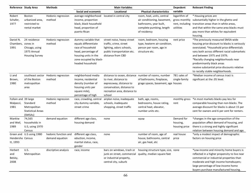
66
Social and economic Locational Physical characteristics
Robert
Schafer,
1977
Boston
urbanized area,
restricted to
rental market
Hedonic regression
method
average neighborhood
income, proportion
black, black household
head, proportion of
puerto Rican
located in central city room, heat, units, central
air conditioning, basement,
bathrooms, year built,
complete pumbing, length
of residency
logarithm of
gross monthly
rent, including
utilities
* Housing prices are
substantially higher in the ghetto and
transition areas than in white areas,
and that within the same area blacks must
pay more than whites for equivalent
housing.
Daniel N.
Chambers,
1991
24 residence
zones in
Chicago, using
1975 Annual
Housing Survey
Hedonic regression
method
dummy variable that
equals differentiate
race of household
head, percentage of
housing units in the
zone occupied by black-
headed household
street noise, heavy street
traffic, crime, street
lighting, odors schools,
public transportation etc.
distance from CBD
room, bedroom, housing
type, heaterm air-condition,
person per room, age in
structure etc.
rent price *The previously measured SMSA-wide
housing price discount to blacks is seriously
overstated; *Household price differentials
vary both across different racial submarkets
and between 1975 and 1979;
*Racially changing neighborhoods near
predominantly black areas
receive substantial price discounts relative
to racially stable neighborhoods.
Li and
Brown,
1980
southeast sector
of the Boston
metropolitan
area
Hedonic regression
method
neighborhood media
income, residential
density (number of
housing units per
square mile),
percentage of high
distance to ocean, distance
to river, distance to
expressway, distance to
conservation, distance to
recreation area, distance to
school
number of rooms, number
of bathrooms, fireplaces,
grage spaces, basement, age
781 sales of
single-family
houses
*Median income of census tract is
significant at the .05 level.
Follain and
Malpezzi,
1981
39 large
Standard
Metropolitan
Statistical Areas
(SMSAs)
Hedonic regression
method
race, crowding, central
city dummy variable,
street crime
airplan noise, inadequate
schools, inadequate
shopping, street traffic
bath, age, rooms,
bedroooms, house rating,
central heat, elevator,
number units etc.
monthly gross
rent
*in most markets blacks pay less for
comparable housing than non-blacks. The
average discount for blacks is about 15 per
cent for owners and 6 per cent for renters.
Mankiw
and Weil,
1989
74,565
households in
U.S, using 1970
Census
demand equation different age class,
housing demand
none none Demand for
housing,
housing price
*changes in the age composition of the
population affect demand of housing, and
there is a strong and highly significant
relation between housing demand and age.
Green and
Hendersho
tt, 1993
U.S using 1980
Census
hedonic function and
demand equation
different age class,
eduction, income,
marital status, race,
gender
none number of room, age of
house, bathrooms, central
air, gas heat, etc
real house
price
*only a modest impact of demographic
factors on housing price
Herbert
and
Belsky,
2008
U.S.
Metropolitan
discriptive analysis race, income bars on windows, trash or
junk on street, commercial
or industrial property,
central city, suburb
housing structure type, size,
quality, median square feet
none *Low-income and minority home buyers is
reflected in a higher propensity to live near
commercial or industrial properties than
moderate and high income homebuyers;
large percentage of low-income home
buyers purchase manufactured housing.
Relevant FindingReference Study Area Methods Main Variables Depedent
variable
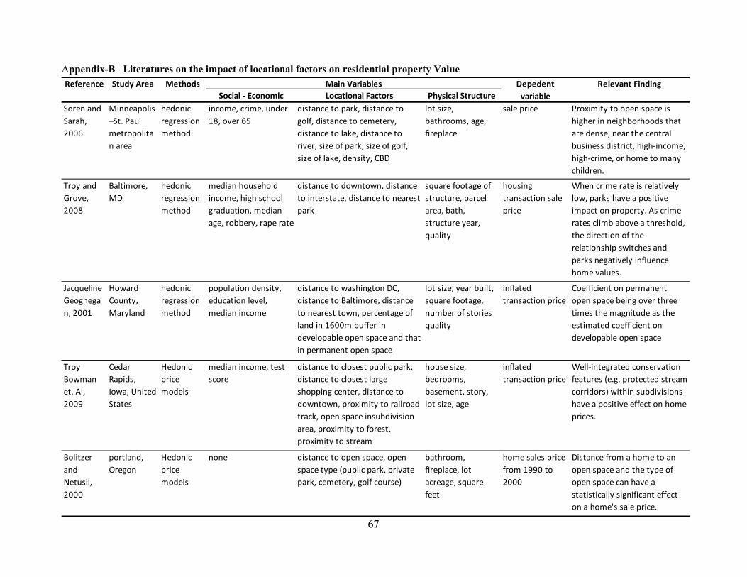
67
Appendix-B Literatures on the impact of locational factors on residential property Value
Social - Economic Locational Factors Physical Structure
Soren and
Sarah,
2006
Minneapolis
–St. Paul
metropolita
n area
hedonic
regression
method
income, crime, under
18, over 65
distance to park, distance to
golf, distance to cemetery,
distance to lake, distance to
river, size of park, size of golf,
size of lake, density, CBD
lot size,
bathrooms, age,
fireplace
sale price Proximity to open space is
higher in neighborhoods that
are dense, near the central
business district, high-income,
high-crime, or home to many
children.
Troy and
Grove,
2008
Baltimore,
MD
hedonic
regression
method
median household
income, high school
graduation, median
age, robbery, rape rate
distance to downtown, distance
to interstate, distance to nearest
park
square footage of
structure, parcel
area, bath,
structure year,
quality
housing
transaction sale
price
When crime rate is relatively
low, parks have a positive
impact on property. As crime
rates climb above a threshold,
the direction of the
relationship switches and
parks negatively influence
home values.
Jacqueline
Geoghega
n, 2001
Howard
County,
Maryland
hedonic
regression
method
population density,
education level,
median income
distance to washington DC,
distance to Baltimore, distance
to nearest town, percentage of
land in 1600m buffer in
developable open space and that
in permanent open space
lot size, year built,
square footage,
number of stories
quality
inflated
transaction price
Coefficient on permanent
open space being over three
times the magnitude as the
estimated coefficient on
developable open space
Troy
Bowman
et. Al,
2009
Cedar
Rapids,
Iowa, United
States
Hedonic
price
models
median income, test
score
distance to closest public park,
distance to closest large
shopping center, distance to
downtown, proximity to railroad
track, open space insubdivision
area, proximity to forest,
proximity to stream
house size,
bedrooms,
basement, story,
lot size, age
inflated
transaction price
Well-integrated conservation
features (e.g. protected stream
corridors) within subdivisions
have a positive effect on home
prices.
Bolitzer
and
Netusil,
2000
portland,
Oregon
Hedonic
price
models
none distance to open space, open
space type (public park, private
park, cemetery, golf course)
bathroom,
fireplace, lot
acreage, square
feet
home sales price
from 1990 to
2000
Distance from a home to an
open space and the type of
open space can have a
statistically significant effect
on a home's sale price.
Reference Study Area Methods Depedent
variable
Relevant FindingMain Variables
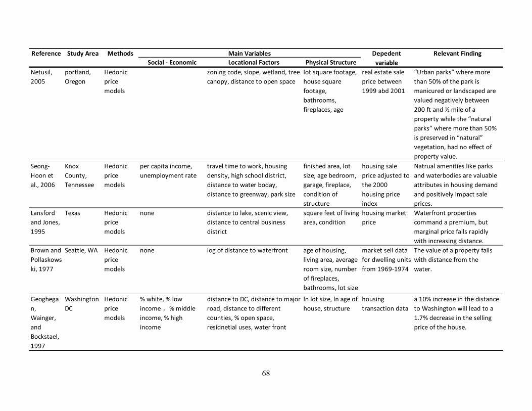
68
Social - Economic Locational Factors Physical Structure
Netusil,
2005
portland,
Oregon
Hedonic
price
models
zoning code, slope, wetland, tree
canopy, distance to open space
lot square footage,
house square
footage,
bathrooms,
fireplaces, age
real estate sale
price between
1999 abd 2001
“Urban parks” where more
than 50% of the park is
manicured or landscaped are
valued negatively between
200 ft and ½ mile of a
property while the “natural
parks” where more than 50%
is preserved in “natural”
vegetation, had no effect of
property value.
Seong-
Hoon et
al., 2006
Knox
County,
Tennessee
Hedonic
price
models
per capita income,
unemployment rate
travel time to work, housing
density, high school district,
distance to water boday,
distance to greenway, park size
finished area, lot
size, age bedroom,
garage, fireplace,
condition of
structure
housing sale
price adjusted to
the 2000
housing price
index
Natrual amenities like parks
and waterbodies are valuable
attributes in housing demand
and positively impact sale
prices.
Lansford
and Jones,
1995
Texas Hedonic
price
models
none distance to lake, scenic view,
distance to central business
district
square feet of living
area, condition
housing market
price
Waterfront properties
command a premium, but
marginal price falls rapidly
with increasing distance.
Brown and
Pollaskows
ki, 1977
Seattle, WA Hedonic
price
models
none log of distance to waterfront age of housing,
living area, average
room size, number
of fireplaces,
bathrooms, lot size
market sell data
for dwelling units
from 1969-1974
The value of a property falls
with distance from the
water.
Geoghega
n,
Wainger,
and
Bockstael,
1997
Washington
DC
Hedonic
price
models
% white, % low
income, % middle
income, % high
income
distance to DC, distance to major
road, distance to different
counties, % open space,
residnetial uses, water front
ln lot size, ln age of
house, structure
housing
transaction data
a 10% increase in the distance
to Washington will lead to a
1.7% decrease in the selling
price of the house.
Relevant FindingReference Study Area Methods Main Variables Depedent
variable
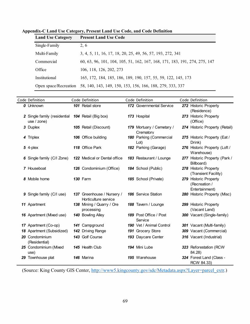
69
Appendix-C Land Use Category, Present Land Use Code, and Code Definition
(Source: King County GIS Center, http://www5.kingcounty.gov/sdc/Metadata.aspx?Layer=parcel_extr.)
Land Use Category Present Land Use Code
Single-Family 2, 6
Multi-Family 3, 4, 5, 11, 16, 17, 18, 20, 25, 49, 56, 57, 193, 272, 341
Commercial 60, 63, 96, 101, 104, 105, 51, 162, 167, 168, 171, 183, 191, 274, 275, 147
Office 106, 118, 126, 202, 273
Institutional 165, 172, 184, 185, 186, 189, 190, 157, 55, 59, 122, 145, 173
Open space/Recreation 58, 140, 143, 149, 150, 153, 156, 166, 188, 279, 333, 337
Code Definition Code Definition Code Definition Code Definition
0 Unknown 101 Retail store 172 Governmental Service 272 Historic Property
(Residence)
2 Single family (residential
use / zone)
104 Retail (Big box) 173 Hospital 273 Historic Property
(Office)
3 Duplex 105 Retail (Discount) 179 Mortuary / Cemetary /
Crematory
274 Historic Property (Retail)
4 Triplex 106 Office building 180 Parking (Commercial
Lot)
275 Historic Property (Eat /
Drink)
5 4-plex 118 Office Park 182 Parking (Garage) 276 Historic Property (Loft /
Warehouse)
6 Single family (C/I Zone) 122 Medical or Dental office 183 Restaurant / Lounge 277 Historic Property (Park /
Billboard)
7 Houseboat 126 Condominium (Office) 184 School (Public) 278 Historic Property
(Transient Facility)
8 Mobile home 130 Farm 185 School (Private) 279 Historic Property
(Recreation /
Entertainment)
9 Single family (C/I use) 137 Greenhouse / Nursery /
Horticulture service
186 Service Station 280 Historic Property (Misc)
11 Apartment 138 Mining / Quarry / Ore
processing
188 Tavern / Lounge 299 Historic Property
(Vacant Land)
16 Apartment (Mixed use) 140 Bowling Alley 189 Post Office / Post
Service
300 Vacant (Single-family)
17 Apartment (Co-op) 141 Campground 190 Vet / Animal Control 301 Vacant (Multi-family)
18 Apartment (Subsidized) 142 Driving Range 191 Grocery Store 309 Vacant (Commercial)
20 Condominium
(Residential)
143 Golf Course 193 Daycare Center 316 Vacant (Industrial)
25 Condominium (Mixed
use)
145 Health Club 194 Mini Lube 323 Reforestation (RCW
84.28)
29 Townhouse plat 146 Marina 195 Warehouse 324 Forest Land (Class -
RCW 84.33)
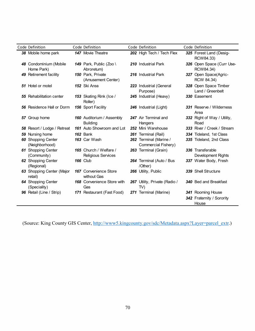
70
(Source: King County GIS Center, http://www5.kingcounty.gov/sdc/Metadata.aspx?Layer=parcel_extr.)
Code Definition Code Definition Code Definition Code Definition
38 Mobile home park 147 Movie Theatre 202 High Tech / Tech Flex 325 Forest Land (Desig-
RCW84.33)
48 Condominium (Mobile
Home Park)
149 Park, Public (Zoo \
Abroretum)
210 Industrial Park 326 Open Space (Curr Use-
RCW84.34)
49 Retirement facility 150 Park, Private
(Amusement Center)
216 Industrial Park 327 Open Space(Agric-
RCW 84.34)
51 Hotel or motel 152 Ski Area 223 Industrial (General
Purpose)
328 Open Space Timber
Land / Greenbelt
55 Rehabilitation center 153 Skating Rink (Ice /
Roller)
245 Industrial (Heavy) 330 Easement
56 Residence Hall or Dorm 156 Sport Facility 246 Industrial (Light) 331 Reserve / Wilderness
Area
57 Group home 160 Auditorium / Assembly
Building
247 Air Terminal and
Hangers
332 Right of Way / Utility,
Road
58 Resort / Lodge / Retreat 161 Auto Showroom and Lot 252 Mini Warehouse 333 River / Creek / Stream
59 Nursing home 162 Bank 261 Terminal (Rail) 334 Tideland, 1st Class
60 Shopping Center
(Neighborhood)
163 Car Wash 262 Terminal (Marine /
Commercial Fishery)
335 Tideland, 2nd Class
61 Shopping Center
(Community)
165 Church / Welfare /
Religious Services
263 Terminal (Grain) 336 Transferable
Development Rights
62 Shopping Center
(Regional)
166 Club 264 Terminal (Auto / Bus
/Other)
337 Water Body, Fresh
63 Shopping Center (Major
retail)
167 Convenience Store
without Gas
266 Utility, Public 339 Shell Structure
64 Shopping Center
(Speciality)
168 Convenience Store with
Gas
267 Utility, Private (Radio /
TV)
340 Bed and Breakfast
96 Retail (Line / Strip) 171 Restaurant (Fast Food) 271 Terminal (Marine) 341 Rooming House
342 Fraternity / Sorority
House
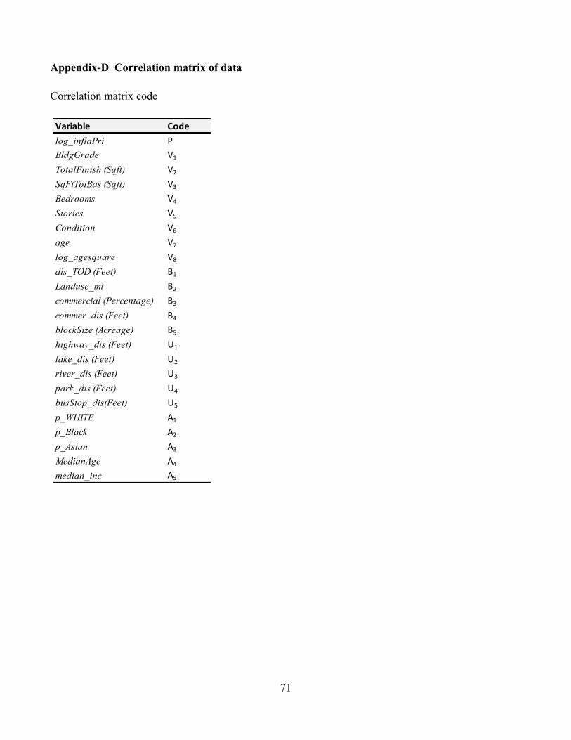
71
Appendix-D Correlation matrix of data
Correlation matrix code
Variable Code
log_inflaPri P
BldgGrade V1
TotalFinish (Sqft) V2
SqFtTotBas (Sqft) V3
Bedrooms V4
Stories V5
Condition V6
age V7
log_agesquare V8
dis_TOD (Feet) B1
Landuse_mi B2
commercial (Percentage) B3
commer_dis (Feet) B4
blockSize (Acreage) B5
highway_dis (Feet) U1
lake_dis (Feet) U2
river_dis (Feet) U3
park_dis (Feet) U4
busStop_dis(Feet) U5
p_WHITE A1
p_Black A2
p_Asian A3
MedianAge A4
median_inc A5
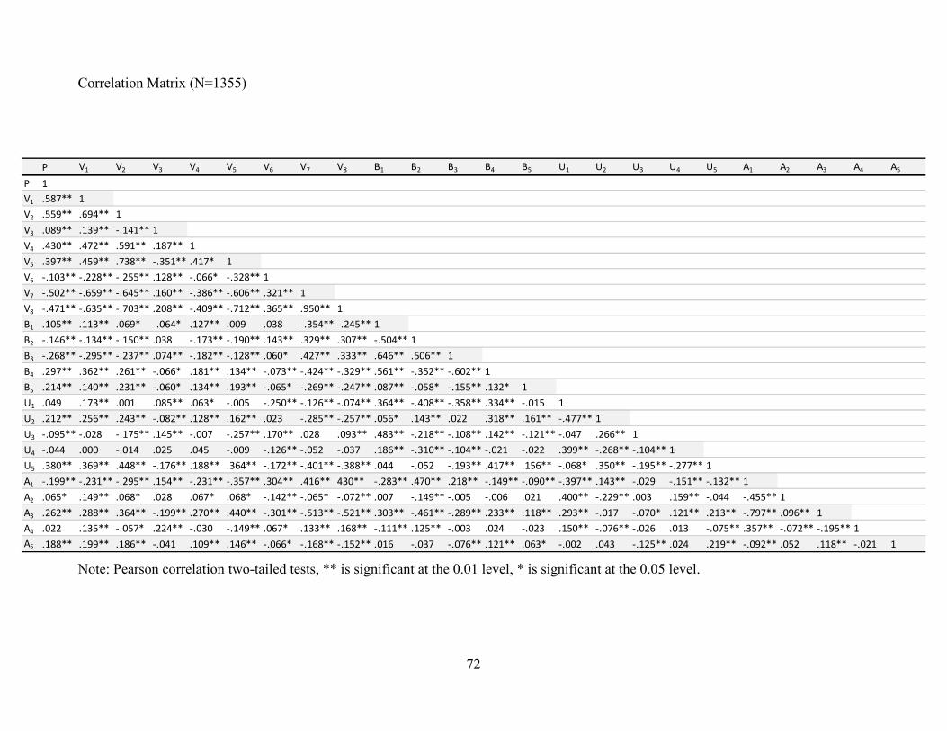
72
Correlation Matrix (N=1355)
Note: Pearson correlation two-tailed tests, ** is significant at the 0.01 level, * is significant at the 0.05 level.
P V1 V2 V3 V4 V5 V6 V7 V8 B1 B2 B3 B4 B5 U1 U2 U3 U4 U5 A1 A2 A3 A4 A5
P 1
V1 .587** 1
V2 .559** .694** 1
V3 .089** .139** -.141** 1
V4 .430** .472** .591** .187** 1
V5 .397** .459** .738** -.351** .417* 1
V6 -.103** -.228** -.255** .128** -.066* -.328** 1
V7 -.502** -.659** -.645** .160** -.386** -.606** .321** 1
V8 -.471** -.635** -.703** .208** -.409** -.712** .365** .950** 1
B1 .105** .113** .069* -.064* .127** .009 .038 -.354** -.245** 1
B2 -.146** -.134** -.150** .038 -.173** -.190** .143** .329** .307** -.504** 1
B3 -.268** -.295** -.237** .074** -.182** -.128** .060* .427** .333** .646** .506** 1
B4 .297** .362** .261** -.066* .181** .134** -.073** -.424** -.329** .561** -.352** -.602** 1
B5 .214** .140** .231** -.060* .134** .193** -.065* -.269** -.247** .087** -.058* -.155** .132* 1
U1 .049 .173** .001 .085** .063* -.005 -.250** -.126** -.074** .364** -.408** -.358** .334** -.015 1
U2 .212** .256** .243** -.082** .128** .162** .023 -.285** -.257** .056* .143** .022 .318** .161** -.477** 1
U3 -.095** -.028 -.175** .145** -.007 -.257** .170** .028 .093** .483** -.218** -.108** .142** -.121** -.047 .266** 1
U4 -.044 .000 -.014 .025 .045 -.009 -.126** -.052 -.037 .186** -.310** -.104** -.021 -.022 .399** -.268** -.104** 1
U5 .380** .369** .448** -.176** .188** .364** -.172** -.401** -.388** .044 -.052 -.193** .417** .156** -.068* .350** -.195** -.277** 1
A1 -.199** -.231** -.295** .154** -.231** -.357** .304** .416** 430** -.283** .470** .218** -.149** -.090** -.397** .143** -.029 -.151** -.132** 1
A2 .065* .149** .068* .028 .067* .068* -.142** -.065* -.072** .007 -.149** -.005 -.006 .021 .400** -.229** .003 .159** -.044 -.455** 1
A3 .262** .288** .364** -.199** .270** .440** -.301** -.513** -.521** .303** -.461** -.289** .233** .118** .293** -.017 -.070* .121** .213** -.797** .096** 1
A4 .022 .135** -.057* .224** -.030 -.149** .067* .133** .168** -.111** .125** -.003 .024 -.023 .150** -.076** -.026 .013 -.075** .357** -.072** -.195** 1
A5 .188** .199** .186** -.041 .109** .146** -.066* -.168** -.152** .016 -.037 -.076** .121** .063* -.002 .043 -.125** .024 .219** -.092** .052 .118** -.021 1
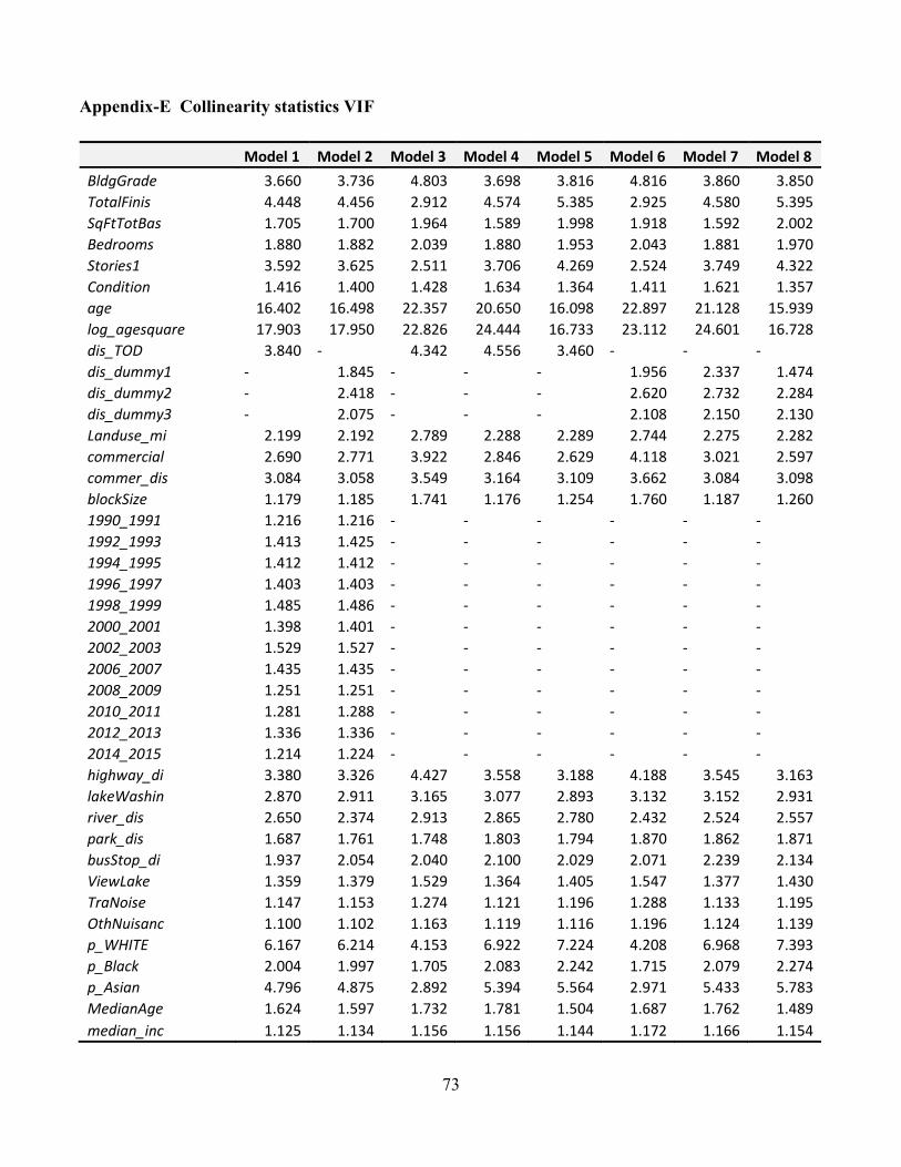
73
Appendix-E Collinearity statistics VIF
Model 1 Model 2 Model 3 Model 4 Model 5 Model 6 Model 7 Model 8
BldgGrade 3.660 3.736 4.803 3.698 3.816 4.816 3.860 3.850
TotalFinis 4.448 4.456 2.912 4.574 5.385 2.925 4.580 5.395
SqFtTotBas 1.705 1.700 1.964 1.589 1.998 1.918 1.592 2.002
Bedrooms 1.880 1.882 2.039 1.880 1.953 2.043 1.881 1.970
Stories1 3.592 3.625 2.511 3.706 4.269 2.524 3.749 4.322
Condition 1.416 1.400 1.428 1.634 1.364 1.411 1.621 1.357
age 16.402 16.498 22.357 20.650 16.098 22.897 21.128 15.939
log_agesquare 17.903 17.950 22.826 24.444 16.733 23.112 24.601 16.728
dis_TOD 3.840 - 4.342 4.556 3.460 - - -
dis_dummy1 - 1.845 - - - 1.956 2.337 1.474
dis_dummy2 - 2.418 - - - 2.620 2.732 2.284
dis_dummy3 - 2.075 - - - 2.108 2.150 2.130
Landuse_mi 2.199 2.192 2.789 2.288 2.289 2.744 2.275 2.282
commercial 2.690 2.771 3.922 2.846 2.629 4.118 3.021 2.597
commer_dis 3.084 3.058 3.549 3.164 3.109 3.662 3.084 3.098
blockSize 1.179 1.185 1.741 1.176 1.254 1.760 1.187 1.260
1990_1991 1.216 1.216 - - - - - -
1992_1993 1.413 1.425 - - - - - -
1994_1995 1.412 1.412 - - - - - -
1996_1997 1.403 1.403 - - - - - -
1998_1999 1.485 1.486 - - - - - -
2000_2001 1.398 1.401 - - - - - -
2002_2003 1.529 1.527 - - - - - -
2006_2007 1.435 1.435 - - - - - -
2008_2009 1.251 1.251 - - - - - -
2010_2011 1.281 1.288 - - - - - -
2012_2013 1.336 1.336 - - - - - -
2014_2015 1.214 1.224 - - - - - -
highway_di 3.380 3.326 4.427 3.558 3.188 4.188 3.545 3.163
lakeWashin 2.870 2.911 3.165 3.077 2.893 3.132 3.152 2.931
river_dis 2.650 2.374 2.913 2.865 2.780 2.432 2.524 2.557
park_dis 1.687 1.761 1.748 1.803 1.794 1.870 1.862 1.871
busStop_di 1.937 2.054 2.040 2.100 2.029 2.071 2.239 2.134
ViewLake 1.359 1.379 1.529 1.364 1.405 1.547 1.377 1.430
TraNoise 1.147 1.153 1.274 1.121 1.196 1.288 1.133 1.195
OthNuisanc 1.100 1.102 1.163 1.119 1.116 1.196 1.124 1.139
p_WHITE 6.167 6.214 4.153 6.922 7.224 4.208 6.968 7.393
p_Black 2.004 1.997 1.705 2.083 2.242 1.715 2.079 2.274
p_Asian 4.796 4.875 2.892 5.394 5.564 2.971 5.433 5.783
MedianAge 1.624 1.597 1.732 1.781 1.504 1.687 1.762 1.489
median_inc 1.125 1.134 1.156 1.156 1.144 1.172 1.166 1.154