THE IMPACTS OF AFFORDABLE LENDING EFFORTS ON HOMEOWNERSHIP ...realestate.wharton.upenn.edu/wp-content/uploads/2017/03/405.pdf · * We thank Freddie Mac and the Zell/Lurie ... we develop

THE IMPACTS OF AFFORDABLE LENDING EFFORTS ON HOMEOWNERSHIP RATES*

Roberto G. Quercia The University of North Carolina at Chapel Hill

George W. McCarthy The Ford Foundation

Susan M. Wachter The Wharton School of the University of Pennsylvania

10/10/2002

Please refer all correspondence to:

Susan M. Wachter Professor of Real Estate and Finance

Real Estate Department Lauder-Fisher Hall, Room 303

University of Pennsylvania, Wharton School Philadelphia, PA 19104 (215) 898-6355 (office) (215) 573-2058 (fax)

[email protected]

* We thank Freddie Mac and the Zell/Lurie Real Estate Center for their support of this research.

ABSTRACT

In this study, we develop and test a methodology to assess the impact of affordable lending efforts on homeownership rates. More narrowly, we examine the impact of using flexible underwriting guidelines, primarily changes in the downpayment and housing burden requirements, on the affordability and homeownership propensities of targeted populations and geographic areas. The impacts of changing these underwriting guidelines are compared with those resulting from lower borrowing costs (interest rates). A variation of the methodology first proposed by Wachter et al. (1995) is used in the analysis. We use the 1995 American Housing Survey (AHS) national core in the analysis. The findings indicate that affordable lending efforts are likely to increase homeownership opportunities for underserved populations, but that impacts may not be felt equally by all groups. Under most affordable products, the impacts on all households, recent movers and central city households are smaller than for other households. The recently introduced affordable products which permit the 3 percent downpayment to come from non-borrower sources, e.g., Freddie Mac�s Alt 97, has the largest impact on the homeownership propensities of all underserved groups, including a 27.1 percent increase in the relative probability of homeownership for young households, a 21.0 percent increase for blacks, and a 15.0 percent increase for central city residents. Consistently, changes in underwriting guidelines are found to have greater impacts than changes in the costs of borrowing for all groups.

1

INTRODUCTION

In recent years, there has been a push to increase home ownership opportunities for groups historically considered underserved. Participants in the mortgage lending industry, such as conventional lenders, government sponsored enterprises (GSEs), and private mortgage insurers (PMIs) have implemented numerous changes in their practices to make borrowing more accessible and affordable to lower income and minority populations than with traditional loan products. Although variations abound, these initiatives can be characterized by targeting of specific populations/geographic areas, and the use of flexible underwriting guidelines and risk mitigating mechanisms, such as counseling. These efforts have been referred to as affordable lending. The affordable lending efforts of so called government sponsored enterprises (GSEs) are of particular importance given the market share of the institutions involved.

The Federal Home Loan Mortgage Corporation (Freddie Mac) and the Federal National Mortgage Association (Fannie Mae), hereafter referred to as the GSEs, are important investors in the conventional market (nongovernment insured or guaranteed loans). By law, all of their loans are at or below the conforming loan limits (Cotterman and Pearce 1994)1. Conventional mortgages have accounted for approximately 99 percent of the total GSE mortgage purchase (CBO 1991). The GSEs control lending risks through underwriting guidelines that have become industry standards. By law, the GSEs need either a minimum 10 percent participation retained by the seller, recourse, or mortgage insurance if borrowers do not provide at least a 20 percent down payment. The GSEs routinely purchase mortgages with downpayments as small as 5 percent. Recently, they have introduced a program linked to automated underwriting that requires a down payment of only 3 percent. The GSEs also establish guidelines for payment-to- income ratios. Generally, the borrower�s housing payments should not exceed 28 percent of gross monthly income2 and the housing payments combined with the borrower�s other monthly obligations, such as credit card and installment debt payments, should not exceed 36 percent, unless there are compensating factors, such as a larger downpayment or demonstrated ability to accumulate savings. 1This limit is the maximum original principal amount for a first lien conventional single-family dwelling. Higher limits are set for two-to-four family dwellings, for multifamily dwellings and for properties located outside the continental U.S. The benchmark used to adjust the limit is the national average one-family price as determined by the Federal Housing Finance Board.

2Housing payments include mortgage principal and interest payments, and payments for property taxes and insurance. Typically, the payments are referred to as PITI.

2

In contrast to traditional loan products, the affordable lending market is

characterized by diversity. Affordable products may include an enhanced marketing strategy to attract loan applicants from targeted groups, or it may involve an automatic second review of some mortgage denials. Most include the use of flexible or nontraditional underwriting guidelines and a homeownership education or counseling requirement. Flexible underwriting guidelines may include elements such as allowing lower downpayments, and higher front-end and back-end ratios, and/or accepting alternative proofs of creditworthiness. For instance, Freddie Mac has three affordable loan products in its Affordable Gold initiative. The Affordable Gold 5 permits a downpayment as low as 5 percent with all funds coming from a borrower�s personal cash. The Affordable Gold 3/2 also permits a downpayment of 5 percent, but only 3 percent must come from a borrower’s own resources. The remaining 2 percent can come from other sources, such as family gifts, government grant, unsecured personal loan and sweat equity. Finally, the Affordable Gold 97 product allows a 97 percent loan to value ratio with the entire 3 percent downpayment coming from the borrower’s personal resources (Stamper 1997). Like Fannie Mae�s Community Home Buyer�s Program, borrowers must be income eligible for the Affordable Gold products. Typically, qualifying borrowers cannot have an income above 100 percent of area median income. Affordable Gold products have no maximum housing expense-to-income ratio (front end) but the monthly debt-to-income ratio (back end ratio) is 38 to 40 percent (Freddie Mac 1999). These products are flexible in that mitigating or compensating factors can be considered in the presence of higher ratios. A recently introduced automated underwriting product permits the required 3 percent downpayment to come from non-borrower sources. As with affordable products, Freddie Mac’s Alt 97 is targeted to borrowers with little savings but good credit histories, however there are no income limits on this program. Because these loans are underwritten through automated underwriting, there are no stated maximum qualifying ratios.

There is some evidence that affordable lending initiatives may be having an impact. Home Mortgage Disclosure Act (HMDA) data show that loans to low income and minority households are growing at a much faster rate than loans to higher income and non-minority households. For instance, the number of loans going to families with incomes at or below 80 percent of the median income for their metropolitan area increased by 38 percent between 1993 and 1997, compared with a 27 percent growth for loans to higher income families (FFIEC 1998). Similar patterns are evident from GSE data on the share of their total business going to low and moderate income households (HUD 1996). All these data suggest that affordable home loan programs may be increasing the flow of funds to nontraditional borrowers and communities. Despite this evidence, the literature lacks an examination of the potential impacts of specific affordable lending products on the homeownership propensities of underserved populations.

This is an important omission since this information is crucial for policy makers, researchers, and others. In designing effective efforts to promote homeownership

3

among nontraditional populations, it is important to know whether downpayment requirements present a higher constraint than do income requirements or the way income constraints increase as downpayment requirements decrease. The GSEs need this information to develop effective affordable loan products. Decision makers at the U.S. Department of Treasury, Housing and Urban Development, and other agencies need to know this information for regulatory purposes. Researchers at several research institutes need this information when evaluating the lending practices of the GSEs. Finally, community groups and community development corporations (CDCs) working to promote affordable homeownership need the information to develop more effective lending efforts.

To fill this void, in this article, we estimate the impacts of different affordable lending products on the homeownership propensities of minority, low-moderate income, central city, recent movers, and young households (head of household 24 to 29 years of age). Also, we assess the impact of changes in borrowing costs relative to the impacts of changing underwriting guidelines. The remainder of the paper is divided into four sections. In the next section, the theoretical underpinnings are presented. Next, the data and methodology are described, including the way key variables are constructed. Following this, the estimation and simulation results are presented. In the final section, implications for policy and research are derived. THEORETICAL UNDERPINNING

Following, Linneman and Wachter (( L-W),1989), Wachter and Megbolugbe (1994) and others, the probability of owning a home [PROB(OWN)] can be expressed as a function of the relative cost of owning versus renting (OWN/RENT), household income (I), the presence of income constraints (IC) and downpayment (DC) constraints, and a number of demographic variables that capture preferences (DEMO).

PROB(OWN) = f (OWN/RENT, I, IC, DC, DEMO) Relative cost of owning versus renting. Several measures have been proposed to capture the relative cost of owning versus renting, including consumption and investment aspects of housing. These are observed rents, rent index (Sheldon 1978) and user cost (Hendershott and Shilling 1982). Goodman (1988) proposes two ratios: a house-specific ratio and a market-specific ratio. The ratio of the market of a house value to its rent value is the house-specific measure (VALRENT). This captures the relationship between consumption and investment characteristics and between renting and owning. With high expected housing price appreciation, which encourages owner-occupancy, the variable will take on high values. Thus, this variable is expected to be positively related to homeownership. The ratio of average owner price in the market to renter price (OWNRENT) in the same market is the measure that controls for the quality of houses across markets. This ratio is expected to have an inverse relationship to owner

4

occupancy, e.g. if the local market has high rents relative to house prices for similar housing, owning is more desirable than renting. Household income and wealth. Household income and wealth play a key role in determining a household’s ability to own a home. We expect both income and wealth to be positively related to the propensity to own. The most desirable measure of income is considered to be the household’s �permanent� income because it reflects longer term income capacity, including that from nonhuman capital. Permanent income, however, is not directly observed. Because a long time series on income for each household is typically not available, the �human capital� approach is used to construct a measure of permanent income (Goodman 1988). Borrowing constraints. L-W are the first to quantify the importance of borrowing constraints on homeownership propensities. They focus on the income and wealth requirements for mortgages that qualify for purchase by Fannie Mae and Freddie Mac. The authors use a four step approach: (1) they estimate the optimal house values for unconstrained households, those households who own homes with market values below what they can afford; (2) they predict the optimal house values for all households; (3) they determine several income and wealth constraint measures on the basis of the difference between the optimal house and the house that can be afforded; and (4) they estimate a logistic model of the probability of homeownership as a function of family income, the relative cost of ownership versus renting, a vector of control variables, and the borrowing constraints. Using data from the 1977 Survey of Consumer Credit and the 1983 Survey of Consumer Finances, the authors find that highly borrowing constrained households were less likely to choose homeownership. Of the two constraints, they find that the wealth constraint variables have larger impacts than the income variables. The authors also contend that the importance of borrowing constraints is likely to diminish with the increasing use of adjustable rate mortgages (ARMs). It should be noted that L-W (as well as all other work based on L-W) does not include information on household indebtedness or credit worthiness. These are important omissions since for many families high levels of indebtedness and/or poor or no credit rating may be the most important barriers to obtaining a loan for home purchase.

A number of other researchers have examined the importance of borrowing constraints. First, Zorn (1989) models the mobility and tenure choice decision subject to income and wealth constraints and suggests that the traditional measure of relative owning/renting costs is not sufficient to describe the tenure choice process. He contends that the tenure decision is better understood as driven by a desire to maximize the level of utility from the overall consumption of housing and nonhousing goods under the two tenure regimes (own/rent). (Add Zorn paragraph)

Second, Haurin, Hendershott, and Wachter (1997) analyze the factors that affect the tenure choice of young adults, highlighting the impact of lender-imposed borrowing constraints. A unique contribution of this study is the use of longitudinal data from the

5

National Longitudinal Survey of Youth (NLSY) for a panel of young households, heads ages 20 to 33 for the years 1985-90. The use of a longitudinal data set allows the authors to model household wealth as an endogenous factor, dependent on savings over time. The authors also check for selection bias when the sample is restricted to unconstrained owners. They apply Heckman’s (1979) method and find no evidence of sample selection bias (the significance level of the inverse Mills ratio (lambda) is only 0.3). The authors find that homeownership tendencies are quite sensitive to potential earnings, the cost of owning relative to renting, and especially borrowing constraints. In their sample, 37 percent of households are constrained even after choosing their loan to value ratio to minimize the impact of the separate wealth and income constraints.

Finally, Linneman, Megbolugbe, Wachter, and Cho (1996) update L-W and estimate the effects of policy changes governing the borrowing constraints and changes in mortgage interest rates both on households’ owning decisions and on the aggregate homeownership rate for the entire U.S. population. They consider 13 policy regimes determined by three levels of downpayment (80, 90 and 95 percent), two levels of front end ratios (28 and 33 percent), and 7 different mortgage interest environments (starting from 7 to 13 percent with incremental increases of 100 basis points). Using the 1989 Survey of Consumer Finance, the authors find that along with permanent income, marital status, and race of household head, borrowing constraints continue to play a significant factor in forming households’ owning decisions. Consistent with L-W, a wealth constraint tends to have a larger and more significant effect than the income constraint. The authors find the impact of wealth constraints to be nonlinear. Increasing the maximum allowable loan-to-value (LTV) ratio is shown to have a larger impact on homeownership rates with higher levels of initial LTV and payment to income ratios. Socio-demographic variables. The use of socio-demographic variables in household demand analysis is extensive and varied (Mayo 1981). These variables include age of head of household, race, and others. Consistent with Wachter and Megbolugbe (1992), socio-demographic factors are included in the present study to control for nonmonotonic effects of socio-demographic effects on permanent income. METHODOLOGY AND DATA

The basic approach to assess the impacts of affordable lending efforts on homeownership rates is to compare homeownership rates under traditional and alternative affordable lending scenarios. More narrowly, the paper offers an assessment of the impacts of changing underwriting guidelines on the homeownership propensity of specific socio-demographic groups while controlling for geographic locations. Of particular interest are the likely changes in homeownership propensities for low and moderate income, black, and young households (head age less than 29 years of age), recent movers, and households living in central cities. A range of impacts due to changes in downpayment and front-end ratio requirements under different interest rate scenarios are estimated.

6

Three steps are taken to determine changes in homeownership propensities that may result from the use of flexible underwriting guidelines. First, key variables are constructed. These include the measures of relative housing prices, permanent income, household wealth, income and downpayment constraint indicators, and the identification of populations of interest. Second, these variables are included in a logistic estimation of the tenure choice equations using different downpayment, front-end ratio and interest rate scenarios and for subpopulations of interest. Third, the changes in the predicted probabilities of ownership under each of the affordable lending scenarios relative to a traditional baseline are calculated for each population of interest.

The data used in the analysis are taken from the 1995 National sample of the American Housing Survey (AHS). The AHS collects data every other year on the nation’s people and their homes (around 42,000 homes). In the 1995 sample, 76 percent of the households had a white non-Hispanic head, 12 percent had a black head of household, 9 percent had a non-black Hispanic head of household. Most of the remaining households are headed by persons of Asian descent.3 1. Variable construction

On the basis of the theoretical presentation above, four types of variables are included in the analysis: relative housing price variables, income and wealth variables, borrowing constraint indicators, and demographic variables. The way each type of variables was constructed is described below.

3The AHS does not provide separate information on the number of black Hispanics. Those identified as blacks probably includes African Americans, black Hispanics, and others.

Relative housing price variables. Following Goodman (1988) and Wachter and Megbolugbe (1992), the value/rent and own/rent ratios are calculated for a national market, with regional variables for both owner and renter housing. This calculation is based on a hedonic price methodology. The dependent variable is the Box-Cox nonlinear transformation of the value or rent of the dwelling unit. The coefficients of the owner/renter hedonic price functions are used to compute marginal trait price schedules, which in turn are used to calculate the value/rent and the own/rent ratios. All relevant housing traits are included in this estimation. Following Goodman (1988), a Box-Cox parameter of 0.3 was used for owner housing and 0.6 is used for renter housing.

The AHS enforces top-coding for many of its variables to protect the identity of its respondents. Of particular importance for this study is the top-coding of house values. Any house value that exceeded $250,000 is coded at that value. Given that the house value is the dependent variable in a number of auxiliary regressions, ignoring the top-coding could introduce truncation bias. The values of top-coded houses are estimated

7

from other data available in the survey.

The original sale price and time of sale is included in the AHS data for each owner-occupied home. Although the sales prices are top coded, there is surprisingly little overlap between top-coded current value and top-coded sales prices. Of the 439 top coded houses in the sample, only 15 had top-coded original sales price. Using the original sales price and the current house value for non top-coded houses, appreciation rates were calculated for all houses in each census region. These are applied to the original sales price for top-coded houses to estimate their current value. Rather than assume an arbitrary value for houses with top-coded sales prices, the estimated appreciation rates are applied to the $250,000 top coded value for these fifteen houses. Although there is some inaccuracy using this technique, the estimated house values more accurately reflect the true house values than more conventional techniques used to adjust for top-coding: choosing an arbitrary single value above the top-code value; or trying to complete the truncated distribution of house prices.

The estimated value/rent ratio is market specific. We divided the sample into 26 markets. Each observation in the sample fall into one of 22 large MSAs or is reported as non-MSA in one of the four census regions. Market baskets are calculated by pooling renter and owner occupied samples. Each �market basket� is defined as the mean of the hedonic characteristics of the housing. The estimated coefficients from the owner occupant hedonic equation are applied to the market basket characteristics to generate a market-specific owner price. Next the coefficients from the rental hedonic equation are applied to the same market basket to generate the renter price. The ratio of the owner and renter prices is the value/rent ratio which varies from market to market but remains constant within markets.

House prices are deflated to allow for comparability of housing in different geographic areas. A deflator is selected based on the median sale price of existing single family homes by MSA as reported by the US Census Bureau (Statistical Abstract 1997, Table 1192, page 720). The deflator used for houses falling outside of MSAs is calculated based on the regional median sale price of existing single family homes for the four census regions defined by the Census Bureau (Statistical Abstract 1997, Table 1191, page 720). We took the 26 median sales prices and regressed them on the mean housing characteristics for each MSA and non-MSA market as derived from our 1995 AHS sample. Using the estimated coefficients, a constant-quality MSA specific housing price deflator is constructed. These constant-quality MSA-specific housing price deflectors are transformed into an index using the national median sales price for existing single family homes as the base (Statistical Abstract 1997, Table 1191, page 720).

The owner/rent ratio is estimated in a similar way. The own/rent ratio is dwelling specific. The owner hedonic price equations are used to compute the marginal trait price schedule and to evaluate the marginal trait price for the given quantity of that trait in each house to give the estimated owner value for that house. For the same house, the

8

renter hedonic price function is used to compute the marginal rent schedule. We evaluated the marginal rental price for the same quantity of the trait in each house to derive the estimated rental value for the house. The ratio of these two calculations is the house specific own-rent ratio. (Refer to the appendix for details and tables.) Household income. Consistent with the literature, permanent income is used in the analysis. The methodology used to estimate permanent income is adapted from the “human capital” approach used in labor economics (Goodman 1988, Wachter and Megbolugbe 1992). In the estimation of permanent income, the dependent variable is a Box-Cox transformation of reported income with lambda equal to 0.5 (which represents a square root transformation). The independent variables in the permanent income equation included education of household head, age, marital status, whether spouse works, region of the country, ethnicity, whether owned home before, and number of cars owned. (Refer to the appendix for details and tables.) Borrowing constraints. The identification of income- and wealth-constrained households under different scenarios is done following Wachter et al. (1995).4 This identification is done in several steps: (1) we estimate household wealth, (2) we estimate the maximum home purchase price for which households could qualify based on traditional income and downpayment requirements, (3) we estimate the level of housing services households desire to purchase, i.e., the optimal home purchase price, (4) we identify unconstrained homeowners as those who chose to own homes with values below the maximum house price these households could have purchased under traditional underwriting requirements, (5) we use the unconstrained sample of home owners to estimate the optimal house equation for the whole sample, and (6) we identify households in the whole sample that were income or downpayment constrained, or both. Unfortunately, although AHS has a direct measure of household income, it lacks a direct measure of household wealth to identify downpayment (wealth) constrained households. However, a three-step approach can be used to estimate wealth from AHS data: (1) income-generating wealth can be estimated econometrically from other AHS data, (2) non-wage assets can be estimated as the difference between the reported total household income and total wage income, and (3) the value of home equity for homeowners can be computed.5

First, following Wachter et al. (1995), an estimate of household wealth is derived econometrically from other AHS data. The AHS includes the variable VOTHER. This

4Two other key constraints are not considered in the analysis. These are back end ratios (total indebtedness) and credit information. These should be considered important omissions if households targeted with affordable lending products are more likely to have excessive debt levels and/or poor credit.

5It is important to note that retirement pensions, an important part of household assets, do not generate income. Our estimates of assets do not include pensions.

9

variable measures income from sources other than wages and salary. Also included in the AHS is a set of five indicator variables denoting the sources of VOTHER income. The potential sources of VOTHER are: social security, alimony, welfare, rental income, and interest income. It should be noted that these are not the only sources of VOTHER as some individuals reported other income and none of these sources were designated. It was assumed that these other sources of VOTHER were asset-generated income.

In order to determine asset-generated income, a linear regression is used to determine the average amount of income generated by each source for those who reported multiple sources of VOTHER. This is done by regressing VOTHER on the set of five indicator variables. For those reporting income from the three non-asset sources: social security, alimony, and welfare, the estimated amount of each income source is subtracted from reported VOTHER. The remainder is considered asset-generated income. For those reporting a single source of VOTHER, the entire amount of VOTHER is assumed to be derived from that source. Using asset specific rates of return, the estimated asset generated income is then capitalized to predict assets. (Refer to the appendix for details and tables.)6

6These non-wage earnings were capitalized using the following method. The composition of the average household portfolio was determined using data provided by the Federal Reserve (1997 Statistical Abstract of the United States, Tables 710, pg. 460 and 777, pg. 512). The average return on this portfolio was calculated as a weighted mean of the appropriate returns provided in Tables 813, pg. 527, 807, pg. 524, and 806, pg. 523. The income flow was divided by the average return to calculate the asset stock.

Second, we assume that non-wage income, e.g. the difference between total family income and total income derived from wages and salary, is asset generated. In order to capitalize this flow into an asset base, we assume the difference is business income. We calculated an average return on business investment based on the reported price to earnings ratio on common stocks (Statistical Abstract of the United States 1997, Table 813). The earnings flow is capitalized into an asset stock using this estimated average return.

Finally, housing equity was estimated by subtracting the reported home price from the principal outstanding on the mortgage(s) held on the house.

The three measures of household wealth, as described above, were used to develop the downpayment (wealth) constraint variable. Housing equity and other wealth estimates were discounted for transaction costs to estimate “liquid” assets. For housing equity and business income, transaction costs of 7% of the house or business value were subtracted from the corresponding wealth estimates. For financial assets, a 3%

10

transaction cost is imposed.

An attempt is made to cross-validate the asset estimates.7 We used information on the distribution of household assets from the tabulations of data from the 1995 Survey of Consumer Finances by the Board of Governors of the Federal Reserve (Kennickell et al. 1997). The Fed estimates include pensions in their measure of household assets and do not discount assets for transaction costs. Our estimates of assets are, on average, around two-thirds of the Fed estimates. This is consistent with the Fed’s estimates that pensions account for about one third of average household portfolios. Further, when we compare our estimates of assets by age groups with those of the Fed, the differences increase with age. In other words, our estimates lag the Fed�s estimates more as household age increases. This is consistent with our failure to account for pensions which would increase as a family ages.

A word of caution is warranted however. A potential problem with the wealth estimation is non-randomness in the error estimation. Several components of wealth estimation are inferred from self-reported data on income and assets. If income is under-reported in the AHS,8 It is likely that the VOTHER variable is under-reported as well. This is a major component of the asset estimation and errors in reporting will be magnified in the capitalization process. On the other hand, another major component of wealth, housing equity, is also derived from reported data on principal outstanding mortgage balances and the value of the home. If house values and mortgage balances are more accurately reported in the AHS data, there will be smaller proportional errors in the wealth estimates of homeowners versus non-owners. The problem is compounded by the possible endogeneity of wealth, e.g. its direct relation to income flows, life cycle effects, and other demographic factors.

A further problem with our wealth estimation is that it fails to take pensions into account. Pensions represent a significant portion of household net worth. While pensions are not generally available to spend on housing, they might be borrowed against to accumulate a downpayment. Indeed, as mentioned above, when we compare our estimates of household assets with estimates provided by the Federal Reserve (which include pensions), our estimates are consistently lower.

In any case, following L-W, families are considered unconstrained if they choose to own homes with values below the maximum house prices these families could have purchased under GSEs’ traditional income and downpayment (wealth) requirements. Dummy variables rather than the variables indicating the size of the gap are used to

7An approach similar to the one described is used by Wachter et al. (1995) to estimate household wealth with AHS data. In their work, Wachter et al. cross-validate their 1989 wealth estimates with data from the 1989 Survey of Consumer Finances.

8AHS codebook, Table 1-2, pg. I-II.

11

identify constrained families because the former is considered more important in mortgage underwriting decisions than the latter. The unconstrained sample of home owners is then used to estimate the optimal home purchase equation.

To obtain the predicted optimal home purchase price for all households, the product of the covariate vector for each household and the vector of estimated parameters from the equation above is calculated. If the predicted optimal home purchase price is less than the maximum house price families can afford based on conventional guidelines, families are considered eligible under the income, downpayment, or both requirements. Otherwise, they are considered constrained by one or both requirements.

Measures of constraints were estimated using different downpayment and front-end requirements and for different interest rate scenarios. Populations of interest. The primary goal of the study is to assess the impact of affordable lending efforts (i.e., changing borrowing constraints) on homeownership rates. The identification of impacts on certain populations is of particular interest. These populations include minority households, low to moderate income households, central city residents, recent movers, and young households (with heads 24 to 29 years of age). These are the populations most likely to be targeted for participation in affordable lending programs. 2. Tenure choice estimation

The above variables were included in the estimation of tenure choice equations for all households, recent movers, and young households. More narrowly, we model the tenure decision (Prob(own)) using a logit estimation, so that Prob(own)= permanent income - transitory income - own/rent + value/rent + age -

household size + married - male +/- blacks +/- Hispanic - income constrained - wealth constrained.

The plus and minus signs in front of the variables represent the expected effect of

the variable on the probability of owning a home. These expected signs are derived from the literature presented above. A note is warranted on the expected signs for blacks and Hispanics. Wachter and Megbolugbe (1992) show negative coefficients for blacks and Hispanics. However, Wachter and Megbolugbe do not include measures of constraints in their estimations. Similarly, Wachter et al. (1996) find that when these variables are omitted, blacks and Hispanics do exhibit lower propensities to own than whites (the reference category). However, controlling for the ability of black and Hispanic households to meet downpayment and monthly payment requirements, Wachter et al. find that these effects are reversed in some of their estimations in Wachter et al (1996). Because of the contradictory evidence in the literature, there are

12

no a-priori expectations on the sign of the black and Hispanic variables.9

The results of the estimation are presented as mean partial derivatives for the full, young, and recent mover samples. The results of estimating the tenure choice equation for other sub-populations such as blacks, central city, and low and moderate income households are also presented for the different downpayment, front-end ratio and interest rate scenarios.10 3. Changes in homeownership propensities

Different underwriting scenarios are modeled to capture the impacts of affordable lending efforts on the homeownership propensities of underserved populations. The baseline and affordable scenarios are presented in Table 1. Two of the alternative scenarios include changes in interest rate regimes. These are included to assess the impacts of changes in the cost of borrowing relative to changes in the underwriting guidelines. Assessment of these relative impacts are used to assess the accuracy of attributing observed homeownership propensities wholly to the latter when in fact changes in interest rate may be partially responsible.

9The number of households with a head of Asian ancestry was too small to obtain meaningful estimates and thus these households were not identified separately.

10 A likelihood ratio test was performed to determine whether dividing the sample into different subpopulations was warranted. The test showed a statistically significant difference (.01 level) between the full sample estimation and the estimation based on segmented samples (e.g. recent mover/non-recent mover, central city/non central city, etc). Different variations of the model were estimated as well. Overall, we found the results to be robust under different model specifications.

In addition to modeling the impacts of affordable lending scenarios, one of the estimations in Wachter et al (1996) is replicated. Studies have generally found a disparity of as much as 50 basis points between fixed rate loans with balances above and below the conforming loan limit (Hendershott and Shilling 1989, ICF 1990, Cotterman and Pearce 1994). This difference is attributed to the GSEs’ lower capital costs as a result of their “agency status”. Removal of this �agency status� through privatization is expected to eliminate this capital cost disparity. This is an important issue in the policy debate over the future of the GSEs. To update prior estimates, the impact of a 50 basis point increase in the interest rate was examined as well.

13

The baseline scenario (28/8/20) is defined as a 30 year fixed rate mortgage at the prevailing market rate of 8 percent (1995).11 A 20 percent downpayment and a 28 percent front-end payment to income ratio are assumed.12 Alternative affordable scenarios include a 5 percent downpayment (33/8/5) such as Freddie Mac’s Affordable Gold 95 loans, 3 percent downpayment from borrower’s asset with a 95 LTV (33/8/3-2) such as Freddie Mac’s Affordable Gold 3/2 loans, and a 0 percent downpayment scenario, where the required 3 percent downpayment is assumed to come from nonborrower sources with a 97 LTV (33/8/0-3) such as Freddie Mac’s Alt 97 loans.13 Also, alternative scenarios include 33 and 38 percent front-end ratios. To capture the impacts of lowering borrowing costs, a 200 basis point reduction in the prevailing rate is considered under two scenarios (28/6/20 and 38/6/3). The impacts on all these affordable lending scenarios on the homeownership propensities of underserved populations are presented below. These include changes in the probability of homeownership for young households, minority, low-moderate income, recent movers, and central city households.

11Although the 20 percent baseline downpayment may be considered too high in today�s market, it is used for consistency and comparison with prior work.

12The average interest rate on conventional mortgages in 1995 was 8.05% as reported in the Statistical Abstract (1997, Table 806, pg. 523). The downpayment and PITI criteria were chosen to conform with conventional mortgages not requiring PMI

13Mortgage insurance is assumed to be equal to one-half percent of the value of the loan, for all loans with downpayment smaller than 20% of purchase price. This is added to the interest rate in estimating front end payments. This is a simplifying assumption since lower downpayment products are likely to require a higher premium.

The basic approach is to estimate baseline models for all households and for each targeted population. The coefficients from these models are applied to the individual characteristics of households to estimate the household level homeownership propensity. Group homeownership propensities are calculated as the mean of corresponding household level propensities. The affordable scenarios are modeled by applying the coefficients from the baseline models to individual level characteristics, including the now less restrictive income and asset constraint measures. As before, the

14

resulting mean household level homeownership propensities are used to estimate group propensities.

Descriptive statistics for the sample are presented in Table 2. In 1995, 65.7 percent of households owned their homes. The average value of their homes was about $105,000, or about 250% of family income. The better part (91.5 percent) of household income is estimated to be �permanent� or consistent with the productivity characteristics of the head of household, while 8.5 percent of income is considered �transitory”. In 1995, the average household head was about 49 years old, lived in a household with 2.64 people, was married or had been married, was male (63 percent), and did not live in a central city (66.6 percent). It is estimated that the average household had assets of about $126,000.

Table 3 reports the percentages of households that are income or wealth constrained under the baseline and affordable underwriting scenarios. In the full sample, about one-ninth of households in the sample had inadequate income to afford a mortgage to purchase their optimal house. About one-third of households had insufficient assets to purchase the same house with a 20% downpayment (baseline 28/8/20). As expected, under the affordable scenarios, the percentages of constrained households decreases. For example, a 2% reduction in the mortgage interest rate loosens the income constraint for 4.1% of households (scenario 1, 28/6/20). As a rule, increasing the allowable front-end ratio decreases the percentage of income-constrained households (scenarios 2-6). However, the positive impact of increasing allowable front-end ratios is counteracted when downpayments are lowered beyond a certain point. When downpayments are reduced from 5 to 3 percent (scenarios 3 and 4 respectively), the percentage of income constrained increases even when holding constant front end ratios requirements. This is because households have to get a larger loan to purchase their optimal house than under the larger downpayment scenario.

Consistent with the literature, the downpayment requirement is a greater detriment to home purchase than the income requirement. Thus, lowering the cost of borrowing does not necessarily allow more people to purchase once the downpayment requirement becomes binding. For instance, although the percentage of income-constrained households decreases as a result of a 200 basis point drop from 8 percent (scenario 4) to 6 percent (scenario 5) in the interest rate, the percent of people that could actually buy a house remained the same because the percentage of downpayment constrained households remained unchanged. This implies that there is a significant overlap between the two constraint measures. Because lack of wealth to meet the necessary downpayment is the dominant constraint, most households that are income constrained are also wealth constrained. However, the reverse is not the case.

REPLICATING WACHTER ET AL (1996)

Two aspects of Wachter et al. were replicated with 1995 AHS data. First, we

15

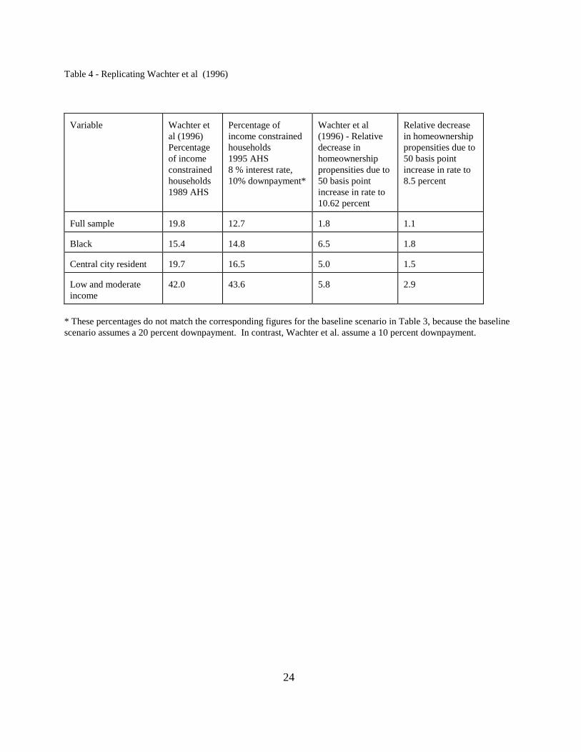
estimated the impacts of a 50 basis point increase in the interest rate expected to result, for instance from GSE privatization, on the incidence of income and wealth constrained households. Second, we estimated the impacts of a 50 basis point increase in rates on the homeownership propensities of targeted populations. Wachter et al (1996) report increases in the number of income-constrained households ranging from 5 to10 percent when the interest rate go from 10.12 to 10.62 percent. Similarly, although somewhat more modest, Table 4 reports that increases in the incidence of income-constrained households range from 1.1 to 2.9 percent when the interest rate goes from 8.0 to 8.5 percent.

To complement the replication of the constraint analysis in Wachter et al., Figure 1 shows the relationship between mortgage interest rates and the incidence of income constrained households at two levels of downpayments. A slight non-linear trend seems apparent, especially at higher levels of loan to value as interest rates increase. This suggests that GSE privatization may have a greater impact than previously thought in the presence of the low downpayment loans widely available today. Wachter et al. (1996) do not capture this non-linear trend.

Consistent with Wachter, et al (1996), a 50 basis point increase in interest rates is expected to decrease homeownership rates across all types of households (Table 4). Using data from 1989, Wachter et al. (1996) report decreases in homeownership propensities ranging from 1.8 to 5.8 percent as a result of an interest rate increase from 10.12 to 10.62 percent. Somewhat more modest, decreases in predicted homeownership rates range from 1.1 to 2.9 percent in relative terms when interest rates increase from 8 to 8.5 percent. Consistent with Wachter et al, blacks, central city, and low-moderate income households are found to experience the greatest negative impacts.

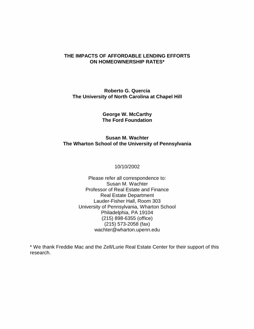
The differences between the effects estimated with 1989 data and those estimated with 1995 data suggest at least two accounts. First, the effect of a given interest rate increment is likely to be higher at higher baseline rates. In other words, the impact of GSE privatization will be larger when interest rates are higher. One would expect smaller effects given the lower 1995 baseline rates. Such a nonlinear relationship between interest rates and homeownership is depicted in Figure 2. As interest rates increase, homeownership rates decrease at an increasing rate. Also, the steeper slope of the 95 percent LTV ratio suggests that as downpayment decreases, interest rate changes have a greater impact on homeownership rates. Second, the increased bifurcation in the national income distribution since the 1980s might have an impact on homeownership. If fewer families are clustered in income levels at which homeownership is a distinct possibility, small changes in underwriting parameters will have smaller relative impacts.

A note is warranted about the way Wachter et al. (1996) estimate homeownership propensities using 1989 AHS data. Wachter et al. use logit coefficients and mean

16

values for covariates to estimate the probability change at covariate means.14 This approach results in higher estimated effects because, in part, of the nonlinearity of the logit function. Thus, because probability density functions are non-linear, estimating marginal changes at covariate means will likely over-estimate actual effects. In contrast, the homeownership probabilities reported in the rest of this article are estimated using the actual individual probabilities of homeownership for each household, for each scenario. The mean of the individual probabilities is reported for each group under study. The reported statistics are weighted using the sample weights provided by AHS. We believe that this is a more accurate measure of the simulated effects. ECONOMETRIC RESULTS

Table 5 presents the model used to estimate the probability of homeownership for all households. Generally, the results conform to those found in other studies of tenure choice (e.g., Wachter and Megbolugbe 1992; Linneman and Wachter 1989). The permanent income component is strongly positively associated with homeownership propensity. The coefficient on transitory income is smaller, negative and significant. The relative cost of ownership is also a strong, negative determinant of ownership, while anticipated capital gains, as captured by the value-to-rent ratio, are positively associated with ownership. Homeownership is statistically significantly associated with age and marital status. Consistent with the findings of other recent studies, homeownership rates fall with the number of dependents in the household. Controlling for borrowing constraints, females, blacks and Hispanics exhibit higher rates of home ownership than whites and males.15

Finally, and importantly for present purposes, the constraint variables have the expected negative signs and are significant. The income constraint term, though statistically significant, tends to have low-magnitude effects; but the downpayment constraint indicator is significant, statistically and substantively. The wealth constraint 14 Wachter et al. (1996) also report unweighted probability changes.

15Additional analysis (not reported) here indicated that there is a high correlation between the incidence of being constrained and being in households headed by a black, Hispanic, or female. This is particularly the case for wealth constrained households. Also, we found that there is a lower correlation between the black, Hispanic and the ever married variables than for whites. This suggests that the positive coefficients of blacks and Hispanics in the estimated model are likely to be due to the inclusion of the constraint variables.

17

has about three times the impact of the income constraint.

The results of estimating the tenure choice equation for black, central city, recent movers, and low-moderate income households are not presented here (available from the authors). Likelihood ratio tests indicate that these bifurcations of the model significantly improve the fit of the data. As a rule, the findings are similar to those discussed above.

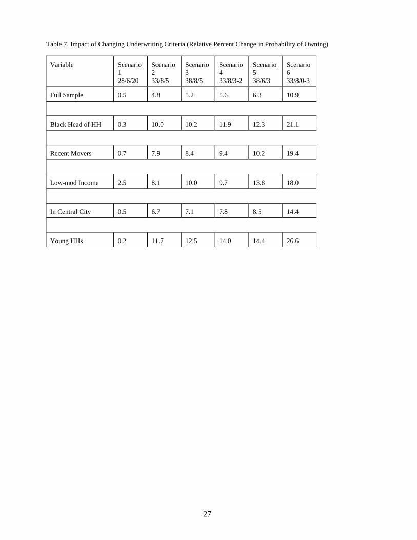
The homeownership propensities for all households and for targeted groups are presented in Tables 6 for the baseline, and affordable scenarios. The impacts of alternative underwriting scenarios on homeownership rates are presented in Table 7. These impacts are captured with the relative changes in homeownership propensities due to shifting from the baseline scenarios to the alternative affordable scenarios. The relative changes are calculated using the mean baseline probability for each targeted group.

As expected, ownership rates are higher for all groups under all affordable scenarios than under the baseline scenario. Overall, the impacts of changing borrowing costs (changes in interest rate) are smaller than those resulting from changing underwriting guidelines. These can be seen in the relative changes from the baseline (28/8/20) to Scenario 1 (28/6/20). Consistent with prior work, changes in downpayment requirements are found to have greater impacts on homeownership propensities than changes in the front-end ratios.

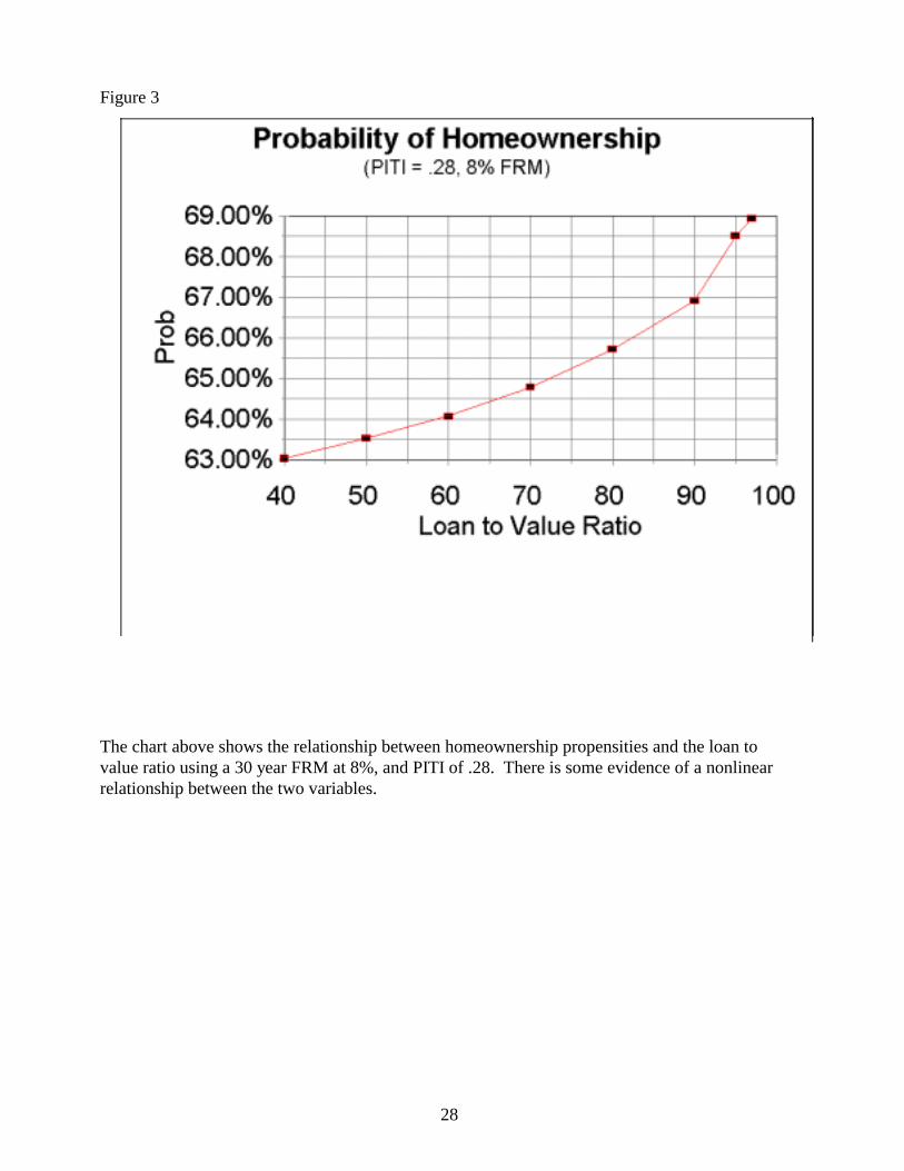
The results indicate some evidence of non-linearity between homeownership propensities and loan-to-value ratios, especially for loans with less than a 10 percent downpayment. Figure 3 shows that there are two inflection points in the relationship between the two variables: at 90 and 95 percent loan-to-value ratios. The probability of homeownership increases significantly with LTVs greater than 90 percent. However, Figure 3 also shows that with LTVs greater than 95 percent the probability of homeownership increases at a decreasing rate. Thus, increasing allowable LTVs is likely to have smaller impacts on the propensity of households to purchase a home once LTVs reach 95 percent than when LTVs are between 90 and 95 percent.

The results also indicate that the impacts of changing underwriting guidelines are not uniform across affordable products. As expected, relative changes in ownership rates are smaller for all households. However, except for the scenario 7 (33/8//0-3), Table 7 suggests that these relative changes may be also smaller for recent movers and central city households than for other households. For instance, under scenarios 2 to 5, these relative changes range from 0.7 to 10.2 for recent movers, and 0.5 to 8.5 for central city households compared with relative changes that range from 0.5 to 12.3 for blacks, and from 2.5 to 13.8 for low and moderate income households. These figures suggest that a product such as Freddie Mac�s Affordable Gold 5 is likely to have a greater impact on the homeownership propensities of blacks that it would have on central city households.

18

Compared with other affordable products, scenario 7 (33/8/0-3) suggests that a

loan product such as the recently introduced Alt 97 and Flex 97, in which the required 3 percent downpayment can come from non-borrower sources, result in the highest predicted ownership rates for all groups. However, such a product also results in smaller relative changes in homeownership propensities for the full sample of households and for central city households. Such a product has the greatest impact on the homeownership propensities of young households (26.6 percent increase in homeownership propensity), black households (21.1 percent increase), and recent movers (19.4 percent increase). This suggest that products like Alt97 and Flex97 may be most appropriate to households with income growth potential (e.g., recent university graduates) but not for all low-moderate income households. IMPLICATIONS FOR POLICY AND RESEARCH

The analysis presented in this study indicates that affordable lending efforts have the potential to increase homeownership opportunities for underserved populations. In particular, the most promising efforts are those that address the lack of adequate savings to make necessary downpayments. The products likely to have the greatest impacts are the recently introduced Alt 97 (Freddie Mac) and Flex 97 (Fannie Mae), that allow the required three percent downpayment to come from non-borrower sources, including unsecured debt. Overall, the impacts of reducing borrowing costs are significantly smaller than those that result from using affordable underwriting guidelines.

Interestingly, the findings suggest that affordable products are not likely to impact

equally all targeted populations. For instance, a product that requires borrowers to make a 3 percent downpayment from their own savings and allows for a 33 percent front-end ratio is likely to increase the relative probability of owning by 6.7 percent among central city households, but 11.7 percent among young households. Thus, narrowly tailored products may be needed to reach specific populations effectively.

Consistent with prior work, lack of the necessary downpayment presents a greater constraint to home purchase than income requirements. However, the findings also suggest the need to define affordability more comprehensively. Homeownership is attainable based not only on the ability to generate the necessary downpayment, but also based on the ability to afford continuing payments on that home after purchase. For instance, the affordability gains that come from reducing downpayments from 5 to 3 percent are counteracted by increases in the number of income constraint households. If one were to include other continuing outlays, for example home maintenance, future capacity of the owners to afford homeownership is diminished further with smaller downpayments. To the extent that affordable homes are older and require more aggressive maintenance, the equity cushion associated with larger downpayments also produces lower capacity risk associated with unforeseen housing expenses.

19

Three other findings are also worth mentioning. The results show nonlinear relationships between homeownership propensities and loan-to-value ratios, between mortgage interest rates and the incidence of income-constrained households, and between mortgage interest rates and homeownership propensities. The first suggests that increasing LTVs beyond 95 percent is not likely to have the same impact on homeownership rates as when loans are made available with LTVs between 90 and 95 percent. The second suggests that the income constraint is likely to be more binding as a result of higher interest rates for the higher LTV loans. Thus, the impact of a 50 basis point rise in the interest rate that may result from GSE privatization may be more significant than previously estimated because of the wide availability of GSE products with 95 percent or higher LTVs. Finally, the slight non-linear relationship between homeownership propensities and mortgage rates suggests that the homeownership impact of GSE privatization would be higher when interest rates are higher.

It is important to note that, even if products are appropriately designed to reach specific populations, the full benefits of these affordable lending efforts may not be fully realized because of supply considerations. Even if households have enough income and wealth to purchase their optimal house, such homes may not be available in the market. If supply considerations are omitted, the potential impacts of affordable lending efforts are likely to be over-estimated. Moreover, the predicted behavior of households is likely to be misspecified because it would ignore likely household behavior in response to a lack of appropriately priced housing. Thus, studies examining the impacts of changing underwriting guidelines in general, and of affordable lending efforts in particular, will need to incorporate supply considerations in the future.

Estimates of the impacts of affordable products, such as the ones in this study, also need to consider the presence of competing loan products in the market. For instance, if the presence of well-established competing products insured by the Federal Housing Administration is not taken into consideration, any estimate of the likely impacts of the GSE affordable products on the homeownership propensities of targeted populations is likely to be overestimated. Thus, the size of the effects estimated in this study is likely to be lower if the presence of competing products, such as FHA�s, are considered.

In addition to the incorporation of supply considerations, the methodology used in the analysis could be improved in a number of ways. These include the inclusion of important information omitted in the present study because of data availability. For instance, most affordable lending efforts, including the Alt97 and Flex97 products, require borrowers to have good credit histories to qualify. In the absence of such information, the reported changes in homeownership propensities overstate the likely impact of affordable lending efforts because not all members of targeted groups have good credit histories. Similarly, omission of information on total household indebtedness is likely to overestimate impacts if households targeted in affordable lending efforts are more likely to have high levels of non-housing debt. Future improvements to the methodology also need to include a more precise estimation of households

20

wealth/assets and incorporating the way changing underwriting guidelines change the cost of owning relative to renting.

21

Table 1. Simulation Scenarios Scenario

PITI

Interest Rate

Downpayment

Baseline Conventional (28/8/20)

28%

8%

20%

1. Conventional (28/6/20)

28%

6%

20%

2. Conventional (33/8/5)

33%

8%

5%

3. Affordable (38/8/5)

38%

8%

5%

4. Affordable (33/8/3-2)

33%

8%

3% (95% loan/value)

5. Affordable (38/6/3)

38%

6%

3%

6. Alt97/Flex 97 (33/8/0-3)

33%

8%

0% (97% loan/value)

22

Table 2. Mean and Standard Deviation of Model Variables Variable

Mean

St. Dev

Own home

0.6526

0.4761

House Value

104,480.70

57,351.16

Household Income

42,341.29

35,233.77

Permanent Income

38,748.26

21,988.82

Transitory Income

3,592.96

32,383.80

Age of Head of HH

48.89

17.193

Own/Rent Ratio

1.4051

0.1214

Valrent Ratio

1.3881

0.0312

Family size

2.64

1.479

Ever Married

0.8377

0.3687

Male Head of HH

0.6353

0.4813

Black Head of HH

0.1162

0.3204

Hispanic Head of HH

0.0874

0.2825

In Central city

0.3336

0.4715

Recent movers

0.3509

0.4749

Assets

125,711.69

231,941.13

23

Table 3. Incidence of Borrowing Constraints

Variable

Baseline Scenario 28/8/20

Scenario 1 28/6/20

Scenario 2 33/8/5

Scenario 3 38/8/5

Scenario 4 33/8/3-2

Scenario 5 38/6/3

Scenario 6 33/8/0-3

Full Sample Income Constrained

11.6

7.5

11.8

8.8

12.2

5.8

12.2

Wealth Constrained

33.8

33.8

16.9

16.9

14.3

14.3

0

Black Head of Household Income Constrained

9.5

6.7

9.6

7.6

9.9

5.4

9.9

Wealth Constrained

45.4

45.4

20.3

20.3

16.5

16.5

0

Recent Movers Income Constrained

10.8

7.2

10.9

8.3

11.3

5.6

11.3

Wealth Constrained

55.4

55.4

28.4

28.4

24.2

24.2

0

Low to Moderate Income Income Constrained

33.8

23.1

34.2

26.5

35.1

18.3

35.1

Wealth Constrained

38.2

38.2

16.6

16.6

13.0

13.0

0

In Central City Income Constrained

11.4

7.7

11.6

8.9

11.9

6.3

11.9

Wealth Constrained

40.2

40.2

18.6

18.6

15.5

15.5

0

Young Households Income Constrained

7.5

4.9

7.6

5.8

8.0

3.9

8.0

Wealth Constrained

63.2

63.2

29.2

29.2

24.6

24.6

0

24

Table 4 - Replicating Wachter et al (1996)

Variable

Wachter et al (1996) Percentage of income constrained households 1989 AHS

Percentage of income constrained households 1995 AHS 8 % interest rate, 10% downpayment*

Wachter et al (1996) - Relative decrease in homeownership propensities due to 50 basis point increase in rate to 10.62 percent

Relative decrease in homeownership propensities due to 50 basis point increase in rate to 8.5 percent

Full sample

19.8

12.7

1.8

1.1

Black

15.4

14.8

6.5

1.8

Central city resident

19.7

16.5

5.0

1.5

Low and moderate income

42.0

43.6

5.8

2.9

* These percentages do not match the corresponding figures for the baseline scenario in Table 3, because the baseline scenario assumes a 20 percent downpayment. In contrast, Wachter et al. assume a 10 percent downpayment.

25

Table 5. Logistic Estimation of Probability of Ownership (Baseline model, all households)

Variable

Coeff.

St. Err.

Prob-val

Intercept

2.1581

0.2700

0.0001

Permanent Income

0.000108

1.62E-6

0.0001

Transitory Income

-0.0001

7.60E-7

0.0001

OWNRENT 16

-5.2742

0.1514

0.0001

VALRENT 17

8.4359

3.7081

0.0229

Age of HH Head

0.0585

0.00119

0.0001

Family size

-0.0249

0.0127

0.0494

Ever married

0.4372

0.0465

0.0001

Male head of HH

-0.4671

0.0350

0.0001

Black head of HH

0.1419

0.0478

0.0030

Hispanic head of HH

0.2812

0.0578

0.0001

Income constrained

-0.5650

0.0504

0.0001

Wealth Constrained

-1.7008

0.0367

0.0001

Number of Observations

40027

-2 log L

Intcpt Only

Int. & cov

Chi-sq pval

51455

25941

0.0001

16 OWNRENT is the ratio of the value of the unit to an owner (assumed to have capitalized the investment value into the house price) to the rental value of the same house based solely on its hedonic characteristics. 17 VALRENT is the ratio of the owned value to the rental value of the average unit in the local market.

26

Table 6. Propensities for Homeownership under Alternate Underwriting Criteria

Variable

Baseline Scenario 28/8/20

Scenario 1 28/6/20

Scenario 2 33/8/5

Scenario 3 38/8/5

Scenario 4 33/8/3-2

Scenario 5 38/6/3

Scenario 6 33/8/0-3

Full Sample

65.7

66.1

68.9

69.1

69.9

69.8

73.4

Black Head of HH

43.8

43.9

48.2

48.4

49.0

49.2

53.1

Recent Movers

38.1

38.4

41.1

41.3

41.7

42.1

45.5

Low-mod Income

47.2

48.4

51.3

52.6

51.8

53.7

55.7

In Central City

50.5

50.7

54.0

54.6

54.5

54.7

57.7

Young HH

32.4

32.5

36.4

36.5

37.0

37.1

41.0

27

Table 7. Impact of Changing Underwriting Criteria (Relative Percent Change in Probability of Owning)

Variable

Scenario 1 28/6/20

Scenario 2 33/8/5

Scenario 3 38/8/5

Scenario 4 33/8/3-2

Scenario 5 38/6/3

Scenario 6 33/8/0-3

Full Sample

0.5

4.8

5.2

5.6

6.3

10.9

Black Head of HH

0.3

10.0

10.2

11.9

12.3

21.1

Recent Movers

0.7

7.9

8.4

9.4

10.2

19.4

Low-mod Income

2.5

8.1

10.0

9.7

13.8

18.0

In Central City

0.5

6.7

7.1

7.8

8.5

14.4

Young HHs

0.2

11.7

12.5

14.0

14.4

26.6

28

Figure 3 The chart above shows the relationship between homeownership propensities and the loan to value ratio using a 30 year FRM at 8%, and PITI of .28. There is some evidence of a nonlinear relationship between the two variables.

29

Figure 1

The graph above shows the relationship between mortgage interest rates and the incidence of income constrained households at two levels of downpayment. A slight nonlinear trend is apparent.

30

Figure 2

There is a slightly nonlinear relationship between interest rates and homeownership. As rates increase the fall in homeownership probabilities increases. The steeper slope of the 95% LTV line shows that as downpayments decrease, interest rates play a larger role in determining homeownership rates.

31

REFERENCES CBO Congressional Budget Office. 1991. “Controlling the Risks of Government-Sponsored Enterprises� April. Cotterman, R.F. and J. Pearce. 1994. The Effects of the Activities of Fannie Mae and Freddie Mac on Conventional Fixed-Rate Mortgage Yields. Working paper. October 29. Engelhardt, G. and G. Mayer. 1995. �House Prices, Savings, and Gifts: The Impact of Liquidity Constraints in the Housing Market.� Paper presented at the AREUEA Meetings, January 1995. FFIEC. 1998. Federal Financial Institutions Examination Council. 8/6/98 Press Release. Freddie Mac. 1999. Federal Home Loan Mortgage Corporation web-page (www.freddiemac.com/sell/alt97) 3/5/99. Goodman, Allen C. 1988. An Economic Model of Housing Price, Permanent Income, Tenure Choice and Housing Demand. Journal of Urban Economics 23:327-53. Haurin, Donald, R.; Patric H. Hendershott, and Susan M. Wachter. 1997. Borrowing Constraints and the Tenure Choice of Young Households. Mimeo. Heckman, James J. 1979. Sample Selection Bias as a Specification Error. Econometrica 47(1): 153-161. Hendershott, Patrick and James Shilling. 1982. The Economics of Tenure Choice, 1955-1979. Research in Real Estate 1:105-33. Kennickell, Arthur B.; Martha Starr-McCluer; and Annika E. Sunden. 1997. Family Finances in the U.S.: Recent Evidence from the Survey of Consumer Finances. Federal Reserve Bulletin (January).

Linneman, Peter; Isaac F. Megbolugbe; Susan M. Wachter; and Man Cho. 1996. Do Borrowing Constraints Change US Homeownership Rates? Mimeo. Linneman, Peter and Susan Wachter. 1989. The Impacts of Borrowing Constraints on Home Ownership. Journal of American Real Estate and Urban Economics Association 17(4): 389-402. Stamper, Michael K. 1997. Revisiting Targeted-Affordable Lending: Fresh Evidence Finds Far Lower Default Rate. Secondary Mortgage Markets 14(3):16-21 (October). Wachter, Susan. 1990. The Limits of the Housing Finance System. Journal of Housing Research 1(1):163-85. Wachter, Susan, James Follain, Peter Linneman, Roberto G. Quercia, and George McCarthy. 1995. �Fannie Mae and Freddie Mac: Implications of Privatization for the Attainment of Social Goals.� Working Paper #218. The Wharton School of the University of Pennsylvania.

32

Wachter, Susan and Isaac Megbolugbe. 1992. Racial and Ethnic Disparities in Homeownership. Housing Policy Debate 3(2): 333-370. HUD. 1996. U S. Department of Housing and Urban Development. Forum on Homeownership Education and Managing Affordable Housing Loans. Washington, D.C: HUD.

33

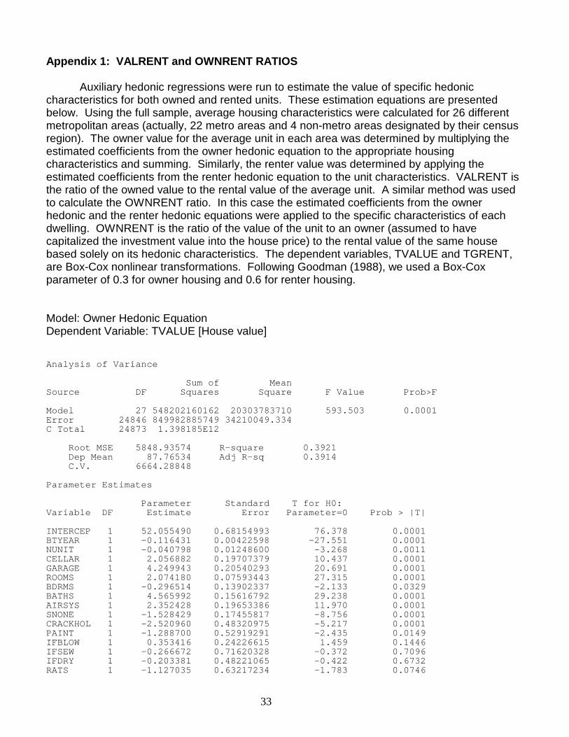
Appendix 1: VALRENT and OWNRENT RATIOS

Auxiliary hedonic regressions were run to estimate the value of specific hedonic characteristics for both owned and rented units. These estimation equations are presented below. Using the full sample, average housing characteristics were calculated for 26 different metropolitan areas (actually, 22 metro areas and 4 non-metro areas designated by their census region). The owner value for the average unit in each area was determined by multiplying the estimated coefficients from the owner hedonic equation to the appropriate housing characteristics and summing. Similarly, the renter value was determined by applying the estimated coefficients from the renter hedonic equation to the unit characteristics. VALRENT is the ratio of the owned value to the rental value of the average unit. A similar method was used to calculate the OWNRENT ratio. In this case the estimated coefficients from the owner hedonic and the renter hedonic equations were applied to the specific characteristics of each dwelling. OWNRENT is the ratio of the value of the unit to an owner (assumed to have capitalized the investment value into the house price) to the rental value of the same house based solely on its hedonic characteristics. The dependent variables, TVALUE and TGRENT, are Box-Cox nonlinear transformations. Following Goodman (1988), we used a Box-Cox parameter of 0.3 for owner housing and 0.6 for renter housing. Model: Owner Hedonic Equation Dependent Variable: TVALUE [House value]

Analysis of Variance

Sum of MeanSource DF Squares Square F Value Prob>F

Model 27 548202160162 20303783710 593.503 0.0001Error 24846 849982885749 34210049.334C Total 24873 1.398185E12

Root MSE 5848.93574 R-square 0.3921Dep Mean 87.76534 Adj R-sq 0.3914C.V. 6664.28848

Parameter Estimates

Parameter Standard T for H0:Variable DF Estimate Error Parameter=0 Prob > |T|

INTERCEP 1 52.055490 0.68154993 76.378 0.0001BTYEAR 1 -0.116431 0.00422598 -27.551 0.0001NUNIT 1 -0.040798 0.01248600 -3.268 0.0011CELLAR 1 2.056882 0.19707379 10.437 0.0001GARAGE 1 4.249943 0.20540293 20.691 0.0001ROOMS 1 2.074180 0.07593443 27.315 0.0001BDRMS 1 -0.296514 0.13902337 -2.133 0.0329BATHS 1 4.565992 0.15616792 29.238 0.0001AIRSYS 1 2.352428 0.19653386 11.970 0.0001SNONE 1 -1.528429 0.17455817 -8.756 0.0001CRACKHOL 1 -2.520960 0.48320975 -5.217 0.0001PAINT 1 -1.288700 0.52919291 -2.435 0.0149IFBLOW 1 0.353416 0.24226615 1.459 0.1446IFSEW 1 -0.266672 0.71620328 -0.372 0.7096IFDRY 1 -0.203381 0.48221065 -0.422 0.6732RATS 1 -1.127035 0.63217234 -1.783 0.0746

34

HOWN 1 0.589608 0.04639363 12.709 0.0001HOWH 1 0.771403 0.06224360 12.393 0.0001NEAST 1 8.818692 0.27877567 31.634 0.0001MWEST 1 1.331769 0.23690448 5.622 0.0001WEST 1 8.519408 0.28938514 29.440 0.0001CCITY 1 -1.769567 0.19395296 -9.124 0.0001NYC 1 10.686391 0.72347781 14.771 0.0001DC 1 17.081803 0.80357348 21.257 0.0001MACA 1 12.210959 0.41530104 29.403 0.0001MAFL 1 3.949704 0.45904560 8.604 0.0001CHI 1 12.858277 0.57574275 22.333 0.0001BOST 1 12.018206 0.92073180 13.053 0.0001

Model: RENTER HEDONIC EQUATIONDependent Variable: TGRENT [Monthly rent]



Model 27 256082209754 9484526287.2 222.191 0.0001Error 14231 607470224586 42686404.651C Total 14258 863552434341


Parameter Estimates


INTERCEP 1 27.912962 0.91516830 30.500 0.0001BTYEAR 1 -0.047990 0.00647160 -7.415 0.0001NUNIT 1 -0.028143 0.00683525 -4.117 0.0001CELLAR 1 2.163207 0.49186794 4.398 0.0001GARAGE 1 5.099900 0.30145463 16.918 0.0001ROOMS 1 2.869400 0.16864908 17.014 0.0001BDRMS 1 -1.252239 0.25305813 -4.948 0.0001BATHS 1 7.715609 0.31002971 24.887 0.0001AIRSYS 1 6.027931 0.31092354 19.387 0.0001SNONE 1 -1.175966 0.35489473 -3.314 0.0009CRACKHOL 1 -1.836763 0.49389000 -3.719 0.0002PAINT 1 -0.247650 0.55478541 -0.446 0.6553IFBLOW 1 1.303750 0.37874398 3.442 0.0006IFSEW 1 -2.200769 0.83137559 -2.647 0.0081IFDRY 1 0.123353 0.54698267 0.226 0.8216RATS 1 -2.995878 0.62880399 -4.764 0.0001HOWN 1 0.562001 0.05860795 9.589 0.0001HOWH 1 -0.424495 0.07348155 -5.777 0.0001NEAST 1 8.089033 0.43186555 18.730 0.0001MWEST 1 0.907860 0.38281277 2.372 0.0177WEST 1 4.723897 0.43932741 10.753 0.0001CCITY 1 -0.203647 0.25647513 -0.794 0.4272NYC 1 9.075298 0.61061615 14.863 0.0001DC 1 15.541091 1.01115635 15.370 0.0001MACA 1 8.783371 0.49208144 17.849 0.0001MAFL 1 7.134414 0.69083841 10.327 0.0001CHI 1 12.446241 0.78742795 15.806 0.0001BOST 1 9.082301 1.04537887 8.688 0.0001

35

Appendix 2: Optimum House Regression Dependent Variable: VALUE95 PROPERTY VALUE (SAMPLE UNIT)- 1995



Model 26 5.3063275E18 2.0408952E17 662.468 0.0001Error 18487 5.6953702E18 3.0807433E14C Total 18513 1.1001698E19


CONST=0

Parameter Estimates


INTERCEP 1 30652 5875.7971336 5.217 0.0001AGE 1 387.782583 124.59452043 3.112 0.0019AGESQ 1 -2.442312 1.16073350 -2.104 0.0354ZINC 1 1.473279 0.02646531 55.668 0.0001ZINCSQ 1 -0.000004580 0.00000014 -31.594 0.0001VALRENT 1 -890920 131435.41296 -6.778 0.0001EVMARR 1 3507.470766 1117.7839100 3.138 0.0017CHILD 1 2217.184754 287.08598273 7.723 0.0001MALE 1 -286.741637 659.42523010 -0.435 0.6637BLACK 1 -11594 1060.7195683 -10.931 0.0001HISPANIC 1 -6484.982809 1356.2262507 -4.782 0.0001OTHER 1 -4584.522179 3094.5884890 -1.481 0.1385EDUC1 1 2646.161031 1585.7059898 1.669 0.0952EDUC2 1 5502.351639 1394.8302688 3.945 0.0001EDUC3 1 11408 1436.2157847 7.943 0.0001EDUC4 1 19928 1514.3886106 13.159 0.0001EDUC5 1 23444 1620.8639792 14.464 0.0001NEAST 1 14830 888.83664042 16.685 0.0001MWEST 1 1311.920646 779.61025228 1.683 0.0924WEST 1 19577 1071.9953844 18.262 0.0001CCITY 1 -4588.281859 854.98554357 -5.367 0.0001NYC 1 12734 2528.5859641 5.036 0.0001DC 1 34351 3368.0871219 10.199 0.0001BOST 1 25154 3468.6367411 7.252 0.0001CHI 1 18186 2491.1898435 7.300 0.0001MACA 1 29481 1602.4809252 18.397 0.0001MAFL 1 9568.656277 1555.0235200 6.153 0.0001

36

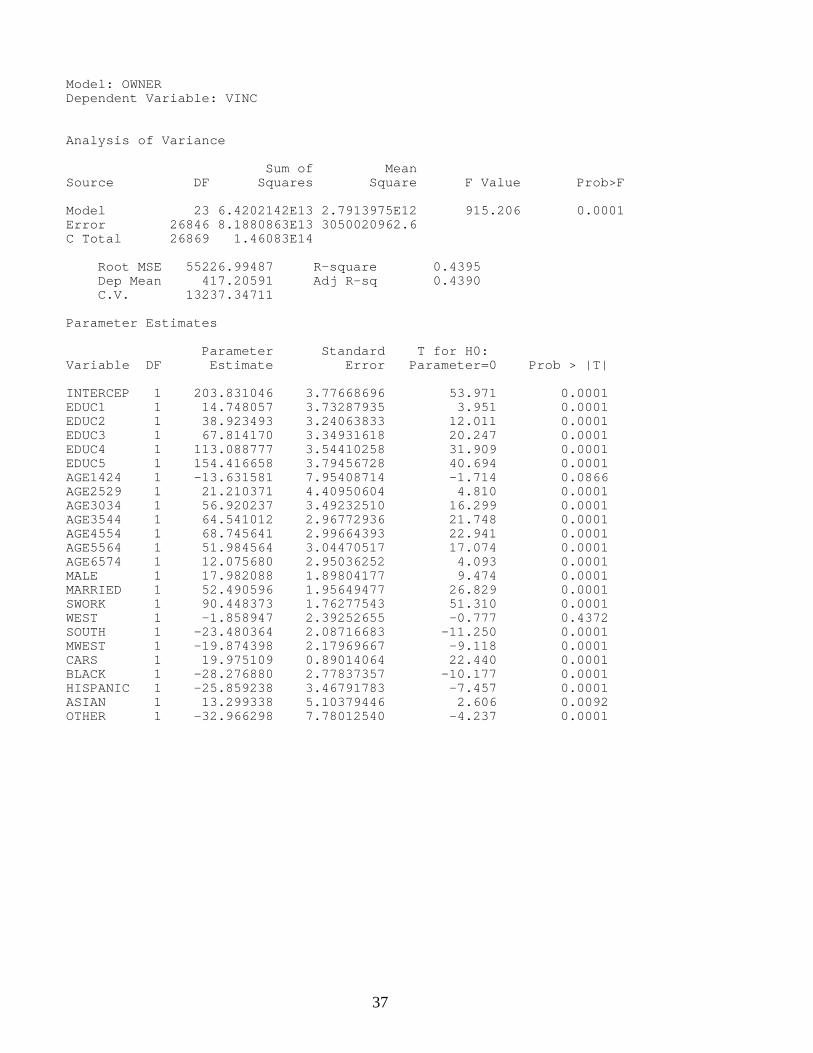
Appendix 3: Human Capital Regressions Model: ALL Dependent Variable: VINC



Model 23 1.0265885E14 4.4634281E12 1587.647 0.0001Error 41158 1.1570944E14 2811347499.2C Total 41181 2.1836829E14


Parameter Estimates


INTERCEP 1 189.400782 2.89600544 65.401 0.0001EDUC1 1 12.453436 2.76785659 4.499 0.0001EDUC2 1 40.753866 2.46465227 16.535 0.0001EDUC3 1 67.529748 2.54360822 26.549 0.0001EDUC4 1 114.359941 2.72773096 41.925 0.0001EDUC5 1 154.712924 3.00279306 51.523 0.0001AGE1424 1 -57.902500 3.29597060 -17.568 0.0001AGE2529 1 -4.414786 2.85937749 -1.544 0.1226AGE3034 1 33.762438 2.65250156 12.729 0.0001AGE3544 1 48.195163 2.37051959 20.331 0.0001AGE4554 1 59.760590 2.44669396 24.425 0.0001AGE5564 1 45.384528 2.55160257 17.787 0.0001AGE6574 1 8.917171 2.50530093 3.559 0.0004MALE 1 21.866744 1.36818055 15.982 0.0001MARRIED 1 64.215091 1.43494940 44.751 0.0001SWORK 1 81.382668 1.37625936 59.133 0.0001WEST 1 -8.115279 1.79407046 -4.523 0.0001SOUTH 1 -18.437868 1.60807091 -11.466 0.0001MWEST 1 -16.692127 1.70868924 -9.769 0.0001CARS 1 22.538237 0.71865388 31.362 0.0001BLACK 1 -33.596156 1.84377715 -18.221 0.0001HISPANIC 1 -32.736502 2.28496656 -14.327 0.0001ASIAN 1 -7.868006 3.63365619 -2.165 0.0304OTHER 1 -23.406597 4.33355467 -5.401 0.0001

37

Model: OWNERDependent Variable: VINC



Model 23 6.4202142E13 2.7913975E12 915.206 0.0001Error 26846 8.1880863E13 3050020962.6C Total 26869 1.46083E14


Parameter Estimates


INTERCEP 1 203.831046 3.77668696 53.971 0.0001EDUC1 1 14.748057 3.73287935 3.951 0.0001EDUC2 1 38.923493 3.24063833 12.011 0.0001EDUC3 1 67.814170 3.34931618 20.247 0.0001EDUC4 1 113.088777 3.54410258 31.909 0.0001EDUC5 1 154.416658 3.79456728 40.694 0.0001AGE1424 1 -13.631581 7.95408714 -1.714 0.0866AGE2529 1 21.210371 4.40950604 4.810 0.0001AGE3034 1 56.920237 3.49232510 16.299 0.0001AGE3544 1 64.541012 2.96772936 21.748 0.0001AGE4554 1 68.745641 2.99664393 22.941 0.0001AGE5564 1 51.984564 3.04470517 17.074 0.0001AGE6574 1 12.075680 2.95036252 4.093 0.0001MALE 1 17.982088 1.89804177 9.474 0.0001MARRIED 1 52.490596 1.95649477 26.829 0.0001SWORK 1 90.448373 1.76277543 51.310 0.0001WEST 1 -1.858947 2.39252655 -0.777 0.4372SOUTH 1 -23.480364 2.08716683 -11.250 0.0001MWEST 1 -19.874398 2.17969667 -9.118 0.0001CARS 1 19.975109 0.89014064 22.440 0.0001BLACK 1 -28.276880 2.77837357 -10.177 0.0001HISPANIC 1 -25.859238 3.46791783 -7.457 0.0001ASIAN 1 13.299338 5.10379446 2.606 0.0092OTHER 1 -32.966298 7.78012540 -4.237 0.0001

38

Model: RENTERDependent Variable: VINC



Model 23 1.5809186E13 687355908201 358.688 0.0001Error 14288 2.7380204E13 1916307643.9C Total 14311 4.318939E13


Parameter Estimates


INTERCEP 1 184.258328 4.15769235 44.317 0.0001EDUC1 1 9.537990 3.62518706 2.631 0.0085EDUC2 1 36.043372 3.35670204 10.738 0.0001EDUC3 1 56.519314 3.45597368 16.354 0.0001EDUC4 1 97.663354 3.82288150 25.547 0.0001EDUC5 1 129.969101 4.60461297 28.226 0.0001AGE1424 1 -32.142762 4.10025003 -7.839 0.0001AGE2529 1 14.205618 3.95178536 3.595 0.0003AGE3034 1 33.351103 3.95462196 8.433 0.0001AGE3544 1 38.599508 3.74729115 10.301 0.0001AGE4554 1 46.447508 4.00975337 11.584 0.0001AGE5564 1 31.083427 4.43550863 7.008 0.0001AGE6574 1 2.044488 4.50586533 0.454 0.6500MALE 1 26.503365 1.73362822 15.288 0.0001MARRIED 1 48.296499 2.02349900 23.868 0.0001SWORK 1 51.732257 2.00262897 25.832 0.0001WEST 1 -11.825672 2.40277710 -4.922 0.0001SOUTH 1 -15.109994 2.27324662 -6.647 0.0001MWEST 1 -20.435812 2.48618246 -8.220 0.0001CARS 1 16.403562 1.16064076 14.133 0.0001BLACK 1 -22.791315 2.17668178 -10.471 0.0001HISPANIC 1 -21.739704 2.66332895 -8.163 0.0001ASIAN 1 -14.204999 4.51057436 -3.149 0.0016OTHER 1 -4.869679 4.43927651 -1.097 0.2727

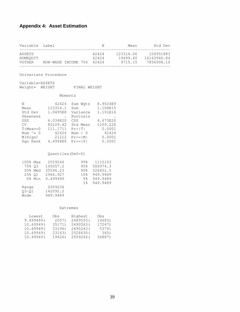
39

Appendix 4: Asset Estimation

Variable Label N Mean Std Dev----------------------------------------------------------------ASSETS 42424 123314.06 104951883HOMEQUIT 42424 19499.60 16163940.84VOTHER NON-WAGE INCOME 704 42424 9715.15 7856998.10----------------------------------------------------------------

Univariate Procedure

Variable=ASSETSWeight= WEIGHT FINAL WEIGHT

Moments

N 42424 Sum Wgts 8.9524E9Mean 123314.1 Sum 1.104E15Std Dev 1.0495E8 Variance 1.101E16Skewness . Kurtosis .USS 6.034E20 CSS 4.673E20CV 85109.42 Std Mean 1109.228T:Mean=0 111.1711 Pr>|T| 0.0001Num ^= 0 42424 Num > 0 42424M(Sign) 21212 Pr>=|M| 0.0001Sgn Rank 4.4996E8 Pr>=|S| 0.0001

Quantiles(Def=5)

100% Max 2559246 99% 111515375% Q3 145057.2 95% 506974.350% Med 35596.23 90% 326451.525% Q1 2964.927 10% 949.94890% Min 9.499489 5% 949.9489

1% 949.9489Range 2559236Q3-Q1 142092.2Mode 949.9489

Extremes

Lowest Obs Highest Obs9.499489( 2057) 2489593( 14683)10.49949( 35171) 2490583( 17247)10.49949( 33196) 2495243( 5376)10.49949( 23163) 2528630( 365)10.49949( 19426) 2559246( 36887)

Documents

THE IMPACTS OF AFFORDABLE LENDING EFFORTS ON HOMEOWNERSHIP ...realestate.wharton.upenn.edu/wp-content/uploads/2017/03/405.pdf · * We thank Freddie Mac and the Zell/Lurie ... we develop