Embed Size (px)
Citation preview

The Impacts of Pore-Scale Physical and Chemical Heterogeneities on
the Transport of Radionuclide-Carrying Colloids
Fuel Cycle Research and DevelopmentNing Wu
Colorado School of Mines
Prasad Nair, Federal POCKevin McMahon, Technical POC
Project No. 13-5008

The impacts of pore-scale physical and chemical heterogeneities on
the transport of radionuclide-carrying colloids
Final Scientific Report
Reporting Period: January 1, 2014 - January 31, 2018
PI: Associate Professor Ning Wu (Colorado School of Mines)
Co-PIs:
Associate Professor Keith Neeves (Colorado School of Mines)
Associate Professor Xiaolong Yin (Colorado School of Mines)
Dr. Jaehun Chun (Pacific Northwest National Laboratory)
Dr. Um Wooyong (Pacific Northwest National Laboratory)
April 2018
Award Number: DE-NE0000719 (Department of Energy)
Submitting Organizations:
Colorado School of Mines
1500 Illinois St., Golden, CO 80401
Pacific Northwest National Laboratory
902 Battelle Blvd, Richland, WA 99354

i
Disclaimer
This report was prepared as an account of work sponsored by an agency of the United States
Government. Neither the United States Government nor any agency thereof, nor any of their
employees, makes any warranty, express or implied, or assumes any legal liability or
responsibility for the accuracy, completeness, or usefulness of any information, apparatus,
product, or process disclosed, or represents that its use would not infringe privately owned rights.
Reference herein to any specific commercial product, process, or service by trade name,
trademark, manufacturer, or otherwise does not necessarily constitute or imply its endorsement,
recommendation, or favoring by the United States Government or any agency thereof. The
views and opinions of authors expressed herein do not necessarily state or reflect those of the
United States Government or any agency thereof.

ii
Executive Summary
This is the final scientific report for the award DE-NE0000719 entitled “The impacts of pore-
scale physical and chemical heterogeneities on the transport of radionuclide-carrying colloids”.
The work has been divided into six tasks and the progress in each is outlined below.
Task 1: The fabrication and characterization of homogeneous microfluidic sediment analog
We developed a microfluidic bead-by-bead assembly platform to fabricate soil analogs
consisting of model grains with homogeneous surface properties. By further integrating a T-
junction droplet generator into the device, we encapsulated and enumerated the effluent in
microliter scale to obtain the average transport behavior of a population of particles. Using the
same device we also measured the individual trajectories of colloidal particles by optical
microscopy. Using the pathlines of individual particles flowing through the pseudo-two-
dimensional bead pack, we were able to extract the tortuosity of differently sized particles and
measure the effects of size exclusion and double layer suppression. Simulations of fluid and
solute transport based on the Lattice Boltzmann Method (LBM) were performed on digitally
reconstructed replicas of the soil analog to aid in the interpretation of the experimental results.
The measured pore scale dynamics of colloid transport such as trajectory lengths were in good
agreement with simulations for small particles in ionic solutions, while larger particles showed
size exclusion effects that are not considered in numerical simulations. Finally, we demonstrated
the profound impact of heterogeneous interfacial properties on colloid transport with an analog
consisting of beads with positive and negative surface charges.
Task 2: The fabrication, characterization, and colloid transport of microfluidic sediment
analogs with chemical heterogeneities
Previous work has primarily focused on physical heterogeneities due to the lack of experimental
models with tunable chemical heterogeneities at the pore-scale. We developed a microfluidic
bead-based fabrication method that are capable to make heterogeneous porous media by
assembling colloidal particles with opposite surface charges so that the chemical heterogeneities
can be precisely defined at the length scale of a single grain. We demonstrated our ability to
make four different configurations of chemical heterogeneities: the alternating horizontal layers,
vertical layers, single patches, and random mixing. We further characterized the spatial
distribution of pore-scale heterogeneities, measured the in situ transport and retention of colloids
in the fabricated porous media using bring-field, fluorescence, and confocal microscopy at the
resolution less than 1 µm. We found that a very small fraction of the positively charged beads
present in the porous medium changes the breakthrough curve dramatically. The overall
deposition coefficient k measured from the colloid retention curves is proportional to the fraction
of the positively charged beads as the extent of unfavorable deposition is negligible. For the first
time, we measured the pore-scale dynamic process of colloidal deposition in situ. The measured
deposition coefficient at the pore-scale, i.e., kpore matches the random sequential adsorption
theory very well.

iii
Task 3: Column-scale experiments - the impact of chemical and physical heterogeneities on
colloid-facilitated cesium transport
Using 1 µm silicon dioxide (SiO2) colloids and cesium iodide (CsI) spiked solution we
investigated the influence of colloid-facilitated Cs transport under relevant physicochemical
porous media conditions in columns packed with glass beads. When the colloids and porous
matrix have similar surface properties at slow pore velocity conditions, contaminants such as Cs
will exhibit no facilitated transport by colloids. This is due to the striping of Cs from the colloids
onto the stationary matrix. We further investigated the influence of hydrophobic/hydrophilic
chemical heterogeneity on transport of Cs and colloids. We found that the transport of colloids
through heterogeneously packed columns is retarded more than through homogenous matrices.
Sequentially layered physical heterogeneity retards colloid transport through the stationary
porous media similar to mixed physical heterogeneities, and the Cs originally adsorbed to the
colloids will be stripped. When a hydrophobic chemical heterogeneity is present in the stationary
matrix, silica-based colloids will be significantly removed due to fast deposition of colloids and
not hydraulically transported through the matrix even with long flushing times unless high flow
rate is maintained.
Task 4: Development of a lattice Boltzmann and random walk particle tracking pore-scale
simulator and its comparison with microfluidic analog experiments
We built a pore-scale numerical simulator to model colloid transport under the influence of
surface charge heterogeneities in the porous media. Our goal is to provide a direct comparison
between the numerical simulation and our microfluidics-based pore-scale experiments in Task 2.
We aimed to use all parameters that can be directly measured from experiments so that there is
no fitting parameter in the simulation. This represents a significant advance in the field of pore-
scale simulation to accurately predict experiments performed at the pore-scale. We first
reproduced the breakthrough curve of electrostatically homogeneous porous media analogue
(PMA). The inlet concentration in our simulation was relaxed by matching the experimental one,
and we obtained a breakthrough curve that agreed well with the experimental breakthrough
curve. This case of electrostatically homogeneous PMA confirmed that our pore-scale modeling
approach using LB and RWPT is applicable to colloid transport in the high Péclet number flow
regime. We then incorporated colloid-surface interaction range and dynamic blocking functions
to simulate irreversible colloid deposition in electrostatically heterogeneous PMAs and obtained
breakthrough curves that are good agreement with those of PMAs.
Task 5: Development of the lattice Boltzmann pore-scale and random walk particle
tracking simulator and its comparison with column experiments
We developed a pore-scale direct numerical model using both LB and RWPT to solve advection-
dispersion of solutes in a bead-packed column, which has been performed in Task 3. Both LB
and RWPT codes have been parallelized to reduce the computational time. The RWPT code
generates tracer concentration profiles at the outlet (i.e., breakthrough curve or BTC). To

iv
generate data that are comparable to the column experiments, image processing routines were
developed to digitalize images of the columns used in the experiments to build the simulation
domain needed by LB and RWPT simulations. The digitalized column contains about 49.5
million voxels (169 × 169 × 1732) and the number of fluid voxels is approximately 10 million.
We first obtained the breakthrough curve of a non-reactive solute (I−) that is in good match with
the experimental data. This model was then extended to simulate equilibrium retardation of Cs+
by adding probabilistic interactions between tracer particles and solid surface. We simulated
laboratory batch experiments and obtained probabilities of adsorption and desorption that
reproduce the experimental partitioning coefficient. Pore-scale direct numerical simulations then
successfully reproduced the retarded breakthrough curve that was in good agreement with the
experimental data.
Task 6: Development of a continuum-scale simulator and its comparison with pore-scale
simulator and microfluidic experiments
We numerically simulated colloid transport and retention in chemically heterogeneous porous
media using one-dimensional advection-dispersion equation. We first obtained the dispersion
coefficient by fitting the experimental data from a homogeneous porous medium that are packed
by carboxyl-functionalized beads only. We then fitted experimental breakthrough curves to find
out the overall deposition coefficients using a dynamic blocking function based on the random
sequential adsorption model. Although the simulations capture the overall trend, they predict a
lesser extent in terms of concentration increase for the latter part of the breakthrough curves. An
inaccuracy in the dynamic surface blocking function, though better than the Langmuirian model,
might be responsible for this discrepancy. In comparison, the pore-scale simulations based on
lattice Boltzmann and random-walk particle tracking capture our experimental results well.

v
Table of Contents
1. Introduction ............................................................................................................................. 1
2. Task 1: The fabrication and characterization of homogeneous microfluidic sediment analog 4
2.1 INTRODUCTION ............................................................................................................ 4
2.2 MATERIALS AND METHODS ..................................................................................... 5
2.3 RESULTS AND DISCUSSION .................................................................................... 10
2.4 CONCLUSION .............................................................................................................. 19
3. Task 2: The fabrication, characterization, and colloid transport of microfluidic sediment
analogs with chemical heterogeneities.......................................................................................... 25
3.1 INTRODUCTION .......................................................................................................... 25
3.2 MATERIALS AND METHODS ................................................................................... 26
3.3 RESULTS AND DISCUSSION .................................................................................... 28
3.4 CONCLUSION .............................................................................................................. 37
4. Task 3: Column-scale experiments: The impact of chemical and physical heterogeneities on
colloid-facilitated cesium transport ............................................................................................... 41
4.1 INTRODUCTION .......................................................................................................... 41
4.2 MATERIALS AND METHODS ................................................................................... 42
4.3 RESULTS AND DISSCUSION ..................................................................................... 45
4.4 CONCLUSION .............................................................................................................. 52
5. Task 4: Development of a lattice Boltzmann and random walk particle tracking pore-scale
simulator and its comparison with microfluidic analog experiments ........................................... 56
5.1 INTRODUCTION .......................................................................................................... 56
5.2 METHODS..................................................................................................................... 57
5.3 RESULTS AND DISCUSSION .................................................................................... 68
5.4 CONCLUSION .............................................................................................................. 71
6. Task 5: Development of a lattice Boltzmann pore-scale and random walk particle tracking
simulator and its comparison with column experiments ............................................................... 73
6.1 INTRODUCTION .......................................................................................................... 73
6.2 METHODS..................................................................................................................... 74
6.3 RESULTS AND DISCUSSION .................................................................................... 82
6.4 CONCLUSION .............................................................................................................. 84

vi
7. Task 6: Development of a continuum-scale simulator and its comparison with pore-scale
simulator and microfluidic experiments ....................................................................................... 87
7.1 INTRODUCTION .......................................................................................................... 87
7.2 METHODS..................................................................................................................... 87
7.3 RESULTS AND DISCUSSION .................................................................................... 90
7.4 CONCLUSION .............................................................................................................. 93

vii
List of figures
Figure 2.1 Configuration of the microfluidic device designed for building the soil analog and
studying in situ colloidal transport. ................................................................................................. 7
Figure 2.2 The porous soil analog formed by trapping PS beads ................................................. 11
Figure 2.3 The cross-sectional and perspective views of the porous medium.............................. 12
Figure 2.4 Numerical simulation with 0, 25, and 50% vertical displacement of beads................ 13
Figure 2.5 Breakthrough measurement with T-junction ............................................................... 15
Figure 2.6 The trajectories of individual particles in the soil analog ............................................ 16
Figure 2.7 The distribution of tortuosity for particles of different sizes in water. ........................ 17
Figure 2.8 Colloids retention in two different types of layered soil analogs ................................ 18
Figure 2.9 The porous soil analog formed by 10 µm aliphatic aminated beads at downstream and
10 µm carboxylated beads at upstream ......................................................................................... 19
Figure 3.1 Configuration of the microfluidic devices designed to pack a binary mixture of beads
into porous media that exhibit chemical heterogeneities and to perform in situ colloid
transport/retention experiments .................................................................................................... 29
Figure 3.2 Different configurations of chemical heterogeneity in the fabricated porous media
packed by a binary mixture of oppositely charged beads ............................................................. 30
Figure 3.3 Radial distribution functions for different bead pairs in a porous medium ............... 31
Figure 3.4 Breakthrough curves for the transport of 0.5 µm caboxylated nanoparticles in
chemically heterogeneous porous media ...................................................................................... 34
Figure 3.5 Retention profile and the corresponding deposition coefficient.................................. 35
Figure 3.6 The evolution of surface coverage on five isolated amine-functionalized beads ........ 36
Figure 3.7 Nanoparticles deposited on one isolated amine-functionalized bead .......................... 36
Figure 4.1 XCT images of columns for homogeneous condition (a, b), sequentially layered
heterogeneity (c, d), mixed heterogeneity (e, f), and chemical heterogeneity (g, h) .................... 46
Figure 4.2 Homogeneous bead column breakthrough curves ....................................................... 47
Figure 4.3 Mixed physical heterogeneity bead column breakthrough curves .............................. 49
Figure 4.4 Sequentially layered physical heterogeneity bead column breakthrough curves ........ 49
Figure 4.5 Chemical heterogeneous bead column breakthrough curves ...................................... 50
Figure 4.6 Initial I breakthrough for homogeneous matrix column, sequentially layered physical
heterogeneity matrix column, mixed physical heterogeneity matrix column, and chemical
heterogeneity matrix column ........................................................................................................ 52
Figure 5.1 Schematics of bead-based microfluidic sediment analogues experiment ................... 57

viii
Figure 5.2 The electrostatically homogeneous PMA with 0% positively charged beads ............. 58
Figure 5.3 The electrostatically heterogeneous PMA with positively charged beads .................. 59
Figure 5.4 The LB velocity field of 0% electrostatically homogeneous PMA ............................. 61
Figure 5.5 The LB velocity fields of electrostatically heterogeneous PMA................................. 62
Figure 5.6 Actual inlet injection concentration ............................................................................. 63
Figure 5.7 Actual inlet injection concentration ............................................................................. 64
Figure 5.8 Comparison of the BTCs between the experiment and simulation ............................. 64
Figure 5.9 Illustration of a tracer falling into the “interception length” ....................................... 65
Figure 5.10 The linear Langmuir adsorption and non-linear RAS model (a) and corresponding
probability models (b). .................................................................................................................. 67
Figure 5.11 The breakthrough curves of electrostatically heterogeneous PMAs ......................... 70
Figure 6.1 The top and bottom images of the bead-packed column. ............................................ 75
Figure 6.2 Procedure of image processing of CT-scanned column images to generate digitized
bead-packed column images (#1590) ........................................................................................... 75
Figure 6.3 Processed images of a bead-packed column are stacked to form a 3D digitalized
column for LB and RWPT simulations ........................................................................................ 76
Figure 6.4 Visualization of z-velocity obtained from LB simulation ........................................... 77
Figure 6.5 Illustration of “pseudo tracer” and “real tracer” implemented in RWPT to simulate the
equilibrium adsorption-desorption. ............................................................................................... 79
Figure 6.6 Simulated adsorption-desorption equilibriums at three different combinations of Pa
and Pd (left), and the equilibrium sorption partitioning coefficient from numerical batch
experiments using the same ratio of a probability of adsorption and desorption (Pa / Pd = 37.04)
(right). ........................................................................................................................................... 79
Figure 6.7 Time-lapse sequence of simulation with Pa = 5.0×10⁻⁴ and Pd = 1.35×10⁻⁵ .......... 81
Figure 6.8 Comparison between the breakthrough curve from RWPT simulation (black) and that
from the experiment (red) ............................................................................................................. 83
Figure 6.9 Simulated BTC (black) for Cesium under equilibrium sorption-desorption relative to
the analytic 1D ADE (DL = 11.85 cm2/day and Rd = 5.4) and the experimental data (red) of the
column experiment........................................................................................................................ 83
Figure 7.1 Comparison between RSA and LA models in the dynamic blocking parameter used in
continuum modeling. .................................................................................................................... 89
Figure 7.2 Dispersion coefficient fitting for a homogeneous porous medium packed by
carboxylated beads only. ............................................................................................................... 91
Figure 7.3 The comparison of breakthrough curves and retention profiles from the continuum

ix
model with pore-scale experiments .............................................................................................. 92

x
List of tables
Table 2.1 Characteristics of the fabricated soil analogs and fluid and colloid transport properties
....................................................................................................................................................... 14
Table 2.2 Statistical information of both pathline length and tortuosity measured in four different
colloidal flow conditions............................................................................................................... 17
Table 3.1 R2 values for each type of bead pairs in the comparison of radial distribution functions
between experiments and simulation ............................................................................................ 32
Table 4.1 Partitioning coefficient (Kd) of cesium, surface area per gram material, and particle
density for glass beads and colloids. ............................................................................................. 45
Table 4.2 Chemical and physical properties of glass bead packed columns ................................ 46
Table 4.3 Model parameters for CDE of aqueous cesium and colloids through columns............ 48
Table 5.1 Dimensions of PMA domain ........................................................................................ 56
Table 5.2 Number of charged beads, on the top and bottom wall, and porosity of PMAs ........... 58
Table 5.3 Parameters of LB simulations ....................................................................................... 60
Table 5.4 Parameters of RWPT simulations ................................................................................. 68
Table 6.1 Parameters of LB simulation of the column experiment .............................................. 76
Table 6.2 Parameters of RWPT simulation of Iodide transport. ................................................... 77
Table 6.3 Sorption portioning coefficient (Kd) of cesium, specific surface area, and particle
density for glass beads. ................................................................................................................. 80
Table 6.4 Parameters of RWPT simulation of the column experiment ........................................ 82
Table 7.1 Deposition coefficient obtained by fitting the colloid breakthrough curves (kθ) and the
retention profiles (k/f) ................................................................................................................... 91

1
1. Introduction
Independent of the methods of nuclear waste disposal, the degradation of packaging materials
could lead to mobilization and transport of radionuclides into the geosphere. This process can be
significantly accelerated due to the association of radionuclides with the backfill materials or
mobile colloids in groundwater.1-2 The transport of these colloids is complicated by the inherent
coupling of physical and chemical heterogeneities (e.g., pore space geometry, grain size, charge
heterogeneity, and surface hydrophobicity) in natural porous media that can exist on the length
scale of a few grains. In addition, natural colloids themselves are often heterogeneous in their
surface properties (e.g., clay platelets possess opposite charges on the surface and along the
rim).3 Both physical and chemical heterogeneities influence the transport and retention of
radionuclides under various groundwater conditions. However, the precise mechanisms how
these coupled heterogeneities influence colloidal transport are largely elusive.4 This knowledge
gap is a major source of uncertainty in developing accurate models to represent the transport
process and to predict distribution of radionuclides in the geosphere.
The objective of this project is to identify the dominant transport mechanisms of colloids in
saturated porous media under the influence of pore-scale physical and chemical heterogeneities.
To achieve this objective, we have developed a microfluidic bead-based fabrication method that
are capable to make heterogeneous porous media by assembling colloidal particles with opposite
surface charges so that the chemical heterogeneities can be precisely defined at the length scale
of a single grain. Although we demonstrated our ability to control several different
configurations of the chemical heterogeneities, we primarily focused on the transport and
retention of nanoparticles in the porous media that were randomly packed by a binary mixture of
oppositely charged beads. We found that a very small fraction of the positively charged beads
present in the porous medium changes the breakthrough curve dramatically. And the overall
deposition coefficient k is proportional to the fraction of positively charged beads present in the
porous medium. More importantly, we measured the in-situ dynamics of nanoparticle deposition
on a single bead for the first time, which provided all necessary parameters that can be used in
pore-scale numerical simulations. We then developed a lattice Boltzmann and random walk
particle-tracking pore-scale simulator simulate our microfluidic experiments based on digital
reconstruction of the fabricated porous media. The faithful comparison between simulations and
experiments including the breakthrough curves, effective retention, and distribution of entrapped
colloids provided a fundamental understanding of colloid transport in heterogeneous porous
media. At the column-scale, we also investigated the influence of colloid-facilitated Cs transport
under relevant physicochemical porous media conditions in columns packed with glass beads
with hydrophobic/hydrophilic chemical heterogeneity. The transport of colloids through
heterogeneously packed columns is retarded more than through homogenous matrices. When a
hydrophobic chemical heterogeneity is present in the stationary matrix, silica-based colloids will
be significantly removed due to fast deposition of colloids and not hydraulically transported
2
through the matrix even with long flushing times. The corresponding simulations based on lattice
Boltzmann and random walk particle-tracking successfully reproduced the experimentally
measured retarded breakthrough curves. Beyond pore scales, we further developed a predictive
continuum-scale simulator that uses the averaged adsorptive properties obtained from the
microfluidic experiments directly without any fitting. Our pore-scale experiments successfully
yielded parameters that can be directly used in both pore-scale and continuum-scale simulations
and the results from those simulations capture key features observed in experiments very well.
The delivery of such capability based on first-principles at the microscopic scale and predictive
at the intermediate scale represents a significant advance towards fully predictive models for
field-scale applications.
This report is the final scientific one for the award DE-NE0000719 entitled “The impacts of
pore-scale physical and chemical heterogeneities on the transport of radionuclide-carrying
colloids”. The work has been divided into six tasks:
Task 1: The fabrication and characterization of homogeneous microfluidic sediment
analog;
Task 2: The fabrication, characterization, and colloid transport of microfluidic sediment
analogs with chemical heterogeneities;
Task 3: Column-scale experiments - the impact of chemical and physical heterogeneities
on colloid-facilitated cesium transport;
Task 4: Development of a lattice Boltzmann and random walk particle tracking pore-
scale simulator and its comparison with microfluidic analog experiments;
Task 5: Development of the lattice Boltzmann pore-scale and random walk particle
tracking simulator and its comparison with column experiments;
Task 6: Development of a continuum-scale simulator and its comparison with pore-scale
simulator and microfluidic experiments.
The progress for each of the above tasks is described in the following sections 2-7.

3
REFERENCES
1. Kersting, A. B., et al., Migration of plutonium in ground water at the Nevada Test Site.
Nature 1999, 397, 56-59.
2. Kanti Sen, T.; Khilar, K. C., Review on subsurface colloids and colloid-associated
contaminant transport in saturated porous media. Advances in Colloid and Interface Science
2006, 119, 71-96.
3. Van Olphen, H., An introduction to clay colloid chemistry: for clay technologists,
geologists, and soil scientists. 2nd ed.; Krieger Pub. Co.: Malabar, Fla., 1991; p xviii, 318 p.
4. McCarthy, J. F.; McKay, L. D., Colloid transport in the subsurface: Past, present, and
future challenges. Vadose Zone J 2004, 3, 326-337.

4
2. Task 1: The fabrication and characterization of homogeneous
microfluidic sediment analog
2.1 INTRODUCTION
Colloids enhance the transport of contaminants such as certain types of radionuclides,1,2 heavy
metals,3,4 and organic substances5,6 by carrying them over long distances in groundwater.
Identifying the transport mechanisms of mobile colloids in the subsurface environment is
essential for predicting the fate and preventing the spread of contaminants. The most common
laboratory method to investigate colloid transport is packed columns of model or natural soils.7–9
The typical data obtained from column experiments are the colloids breakthrough curves, which
measure the population dynamics of colloids exiting the column over time, and the end-point
retention profile, which measures the colloids adsorption in the column7 after sample
dissection.10,11
An alternative to measuring fluid and solute transport macroscopically is to fabricate porous
media analogs (PMA) in transparent substrates. PMA are often referred to as "micromodels" and
are typically made of glass, silicon, or polymers with pores sizes ranging from 1–100 µm and
overall dimensions on the order of millimeters to centimeters.12 PMA in geologically-inspired
materials include functionalization of pore walls with clays,13 wet etching channels directly into
calcite,14 and laser etching into shale.15 The pore networks of these models can consist of
periodic features such as arrays of polygons,16 random networks with statistically similar
porosities and permeabilities of real rocks,17 or replicas of real rock pore spaces based on
imaging data.18 PMA have been particularly useful in visualizing and simulating water,
surfactant, and polymer flooding of oil-saturated pore networks that mimic sedimentary rock.17–
21 Recently, porous networks with dimensions in the sub-micrometer range have been developed
to model liquid-gas flows in shale and tight gas sands.22,23
Although PMA with a continuous solid phase and a series of interconnected channels mimic the
pore space of many resource-rich rocks in deep underground, contaminants that are of most
concern to human health usually reside the shallower subsurface where soils are the dominating
media as unconsolidated, rough, spherical, and micrometer- to millimeter-sized grains. As such,
bead-based or post-based PMA are potentially a better model for measuring colloid transport in
soils.24 For example, the influence of colloid size on dispersion has been measured in
polydimethylsiloxane (PDMS) and silicon pillar based micromodels.25,26 Studies in a glass-bead
PMA show that rod-shaped particles are more likely to attach to the beads than spherical ones
due to local charge heterogeneity and surface roughness.27 In unsaturated porous media, bead-
based PMA show that the adsorption of colloids at air-liquid interfaces as a function of their
wetting properties, surface charge, and the ionic strength of the solution.28–30 In these PMA
studies, individual particle trajectories and adsorption kinetics were observed, but the average

5
transport properties of a large population of particles were not collected. This is possibly due to
the challenge of collecting and analyzing the effluent of PMA since the total volumes are on the
order of nano- to micro-liters. An important property of natural soils is the heterogeneity of
interfacial properties such as charge, wettability, and chemical functionality between grains.30
Yet, unlike the bead-based proteomics and genotyping methods,31–33 the existing work has not
fully exploited a distinct advantage of the beads-based soil analogs, namely each bead can have
its own interfacial properties.
To address the shortcomings described above, we developed a bead-by-bead assembly platform
to fabricate soil analogs. By integrating a T-junction droplet generator into the device, we
encapsulated and enumerated the effluent in microliter scale to obtain the average transport
behavior of a population of particles. Using the same device, we also measured the individual
trajectories of colloidal particles by optical microscopy. Simulations of fluid and solute transport
based on the Lattice Boltzmann Method (LBM) were performed on digitally reconstructed
replicas of the soil analog to aid in the interpretation of the experimental results. The measured
pore scale dynamics of colloid transport such as trajectory lengths were in good agreement with
simulations for small particles in ionic solutions, while larger particles showed size exclusion
effects that are not considered in numerical simulations. Finally, we demonstrate the profound
impact of heterogeneous interfacial properties on colloid transport with an analog consisting of
beads with positive and negative surface charges.
2.2 MATERIALS AND METHODS
Materials
Polydimethylsiloxane (PDMS) was from Dow Corning (Sylgard 184, Midland, MI). Mineral oil
and cyclopentanone (≥99%) was from Sigma Aldrich (St Louis, MO). 1H-1H-2H-2H-
perfluorooctyltrichlorosilane was from Gelest (Morrisville PA). Photoresist (KMPR1010 and
KMPR1050) was from MicroChem (Newton, MA). Developer (AZ300 MIF) was from AZ
Electronic Materials (Somerville, NJ). 0.5 µm carboxylated yellow-green (505/515) particles, 1
µm sulfate yellow-green (505/515), 15 µm blue (365/415), 10 µm crimson (625/645) fluorescent
polystyrene (PS) microspheres and 10 µm aliphatic amine latex beads were from Life
Technologies (Carlsbad, CA). 3 μm carboxylated yellow-green (480/501) fluorescent PS
microspheres were from Magsphere Inc. (Pasadena, CA). Three-inch silicon wafers were from
Silicon Inc. (Boise, ID). Gauge 30 Tygon tubing was from Saint-Gobain North America (ID =
0.01”, OD = 0.03”, Valley Forge, PA). Biopsy punch (0.75 mm) was from World Precision
Instrument (Sarasota, FL).
Device fabrication
Microfluidic channels were defined in PDMS using standard soft lithography techniques.34 A
two-layer photolithography procedure was used to create channels with two different heights on

6
the master. For the first layer, KMPR1010 was spin coated at 3000 rpm for 40 sec, soft baked for
6 min at 100ºC, exposed through a photomask (CAD/Art service, Bandon, Oregon) to UV light
(200 W, 365–405 nm exposure) in a Karl Suss MJB-3 Mask Aligner (Sunnyvale, CA) at a dose
of 10 mW/cm2, and hard baked for 2 min at 100ºC. For the second layer, KMPR 1050 was
diluted to 40 wt% solids in cyclopentanone and spun at 4000 rpm for 40 sec. The same soft bake,
exposure, and hard bake procedures were followed. The photoresist master was made
hydrophobic by incubation with 1H-1H-2H-2H-perfluorooctyltrichlorosilane for 24 h under
vacuum. To make the microfluidic device, PDMS (5:1 polymer vs. curing agent in mass) was
poured over the master and cured for 4 h at 80 ºC. The devices were then peeled off from the
master and plasma bonded on a glass slide. Both the inlet and outlet holes were made with 0.75
mm punch. The detailed fabrication conditions for heterogeneous soil analog channels are
discussed in supplemental materials.
Device operation
Figure 2.1 shows a schematic of the device. It was operated in two modes: the bead filling and
colloid transport mode. In the bead filling mode, a dilute suspension (5×10⁵/ml) of 15 µm beads
was introduced through inlet a. All other inlets and outlets except e were blocked. The beads
were trapped at barrier d, where the channel height is reduced from 21 μm to 12 μm. As beads
were trapped, they formed a porous medium that grew upstream (Supplementary Video 1). For
the layered packing of carboxyl- and amine-functionalized beads in the chemically
heterogeneous soil analog, we injected them sequentially. Note that the channel height was
slightly larger than the diameter of the beads. Therefore, the beads packed pseudo-two-
dimensionally into a porous soil analog that was 840 μm in width, 21 µm in height, and 500–
2000 µm in length. In the colloid transport mode, suspensions of fluorescent particle (0.5, 1, and
3 µm) were injected through inlet b. Since the pore volume was small (~10 nL), collecting fluid
from the outlet of the device was not feasible when trying to measure the transient in colloid
breakthrough. Instead, we placed a T-junction droplet generator downstream at position f to
encapsulate the effluent colloids. DI water entered from inlet c to stabilize droplet generation
before colloids entered. Mineral oil was injected from inlet e and used as the continuous phase.
The aqueous solution emanating from the soil analog is the dispersed phase. For capillary
numbers / 0.01aC Uµ γ= < (where µ is dynamic viscosity, U is velocity, and γ is interfacial
tension), the dispersed phase forms into droplets, where individual particles are encapsulated.35–
37 The droplet size depends on the flow rates of two phases and the channel sizes,
L/W = 1 + αQin/Qout (2.1)
where L is the length of droplet slug, W is the width of the channel, Qin and Qout are the flow
rates of the dispersed and continuous phases, and α is an order one constant.24 We adjusted the
oil flow rates to control the droplet diameter at around 300 μm. Downstream of the T-junction
the channel was expanded from 200 µm to 400 μm to reduce the droplet velocity allowing for
real-time imaging. By taking both fluorescent and bright-field images, the number of colloidal
particles in each droplet and droplet volumes were measured.

7
Figure 2.1 Configuration of the microfluidic device designed for building the soil analog and
studying in situ colloidal transport. (i) The top view; a and b are the inlets for flowing PS beads
and colloidal dispersion into the device; c is the inlet for DI water used to wet the fabricated
porous medium when we switch from the bead-filling mode to colloid-transport mode; d
represents the height barrier (e.g., 10µm) where large (e.g., 15 μm) PS beads are trapped and
packed into the soil analog; e is the inlet for mineral oil; f is the T-junction where the colloidal
solution passing through the soil analog forms individual droplets in the oil phase; g is a
gradually expanded channel that slows down the droplet flow, which facilitates counting the
number of colloidal particles in each droplet. (ii) The side view of the height barrier h. (iii)
Schematics of the soil analog packed by beads ideally. (iv) The T-junction, where the gray
indicates mineral oil, and the white droplets represent colloidal solution that passes through the
porous medium. Green dots inside the droplet represent fluorescent particles.
Identification of bead location
The positions of individual beads in the soil analog were determined by stitching a series of
images together using a 20X objective (field of view = 440 μm × 325 μm) on an inverted
microscope (IX81, Olympus) with a 16-bit CCD camera (ORCA-R2, Hamamatsu). For a 1000
μm long soil analog, 15 images were stitched together using the ImageJ macro stitching.38 A
custom MATLAB script identified the x and y coordinates of the center of each bead using the
following steps: (i) a Canny algorithm39 located the edge of each bead; (ii) a first filtration
operation eliminated any debris or imaging artifacts with a circumference larger than 51 μm; (iii)
features remaining after filtration were filled and a second filtration operation eliminated debris

8
or imaging artifacts with areas less than 31 μm2 or larger than 104 μm2; (iv) a third filtration
operation eliminated debris or imaging artifacts with circularity larger than 0.9. Circularity is
defined as P2/4πA, where P is the perimeter and A is the object area,40 and (v) the imfindcircles
command identified the coordinates of the center of each bead. For the heterogeneous bead
packing, one extra step was added before we run the Canny algorithm. Since we have two
different types of beads, the polycrop command was used to define the region of interest for the
carboxyl-functionalized beads first. The area of other beads was then filled with black pixels.
This operation kept the beads at the same location in the original image. We run the image
processing program for each section of beads first and then combined them to obtain the center
positions of all beads in the whole porous medium.
Measurement of hydraulic permeability
A reservoir of deionized water was connected to inlet b of the device with 30 gauge tubing and
raised 20–60 cm above the device to establish the inlet pressure head. The device for
permeability measurements was similar to that in Figure 2.1, but without the droplet generator.
The outlet channel f’ was connected to 30-gauge tubing placed at the height of the device and
open to the atmospheric pressure. The linear velocity of water was measured by tracking the
meniscus in the outlet tubing for 1 minute. It was then converted to a volumetric flow rate Q
using the cross-sectional area of the tubing. Each pressure drop, ΔP, was repeated in triplicate.
The total hydraulic resistance of the device, R, was calculated by
R=ΔP / Q (2.2)
The total resistance includes the resistance of tubing Rt, the pre/post-analog channel Rc, and the
soil analog Rp connected in series. Rt, and Rc were calculated by:41
(2.3)
(2.4)
where Lt and r are the length and radius of the tubing, respectively. Lc, Wc, and Hc are the length,
width, and height of the pre/post-analog channel. By subtracting Rt and Rc from the total
resistance R, we can obtain the resistance of the soil analog Rp, which is related to the
permeability κ by
(2.5)
where Lp, Wp, and Hp are the length, width, and height of the analog.
Measurement of the colloid population dynamics
The zeta potentials of the particles were measured using ZetaPALS (Holtsville, Brookhaven
Instruments Corporation, NY). Suspensions of particles in DI water were injected at a flowrate of
1 nL/sec through inlet b (Figure 2.1). Mineral oil was injected into the oil inlet e at a flowrate of
4
8t
t
LR
r
µ
π=
( )3
12
1 0.63 /
cc
c c c c
LR
W H H W
µ=
−
p
p p p
L
W H R
µκ =

9
1.6 nL/sec. The colloidal particles emanating from the soil analog were emulsified at the T-
junction. Due to the expansion in channel width at g, the droplet flow velocity was reduced by
half and images of individual droplets were taken in both fluorescent and bright-field modes. A
custom MATLAB script was used to enumerate the number of particles in each droplet using the
following procedure: (i) the im2bw command turned the gray scale image to black and white, and
a contrast threshold is set to ensure all the fluorescent particle turned to white dots, (ii) the
bwboundaries command detected the edge of each white dot and counted their total number.
Trajectory of individual particles and calculation of tortuosity
At a volumetric flow rate of 1 nL/sec, the trajectories of 0.5, 1, or 3 µm particles were measured
by epifluorescence microscopy (20X, NA 0.45) with an exposure time of 500 ms. These imaging
conditions yielded pathlines whose lengths were measured to calculate tortuosity. The diffusion
coefficient of the particles was calculated using the Stokes-Einstein equation: D = kBT / 6πµa,
where kB is the Boltzmann constant; T is absolute temperature; and a is the particle radius. The
Peclet number was defined based on a length scale of porous medium as Pe = Ud/D, where d is
the characteristic length of the porous medium (i.e., the bead diameter); U is the superficial
velocity of the fluid; and D is the colloid diffusion coefficient. The tortuosity was defined by τ =
La / Le, where La and Le are the arc-length and end-to-end distance of the trajectory.
Colloids retention on chemically heterogeneous soil analog
The chemically heterogeneous soil analog was assembled from two types of 10 μm beads
functionalized with carboxyl and amine groups, respectively. We arranged their packing in two
ways. The aliphatic amine beads first packed into a 500×840 (L×W) μm2 rectangular layer,
followed by another layer of carboxylated beads with 500×840 μm2, and vice versa. After the
soil analog was formed, 1 μm particles at the concentration of 0.054 mg/mL were introduced at 2
nL/s for 2 hours and followed by DI water flush at the same rate for another 2 hours. During the
experiment, both fluorescence and bright-field images were taken. A custom MATLAB script
was used to calculate the mean fluorescence intensities at specific regimes over time. For a 16-bit
grayscale image, each pixel was associated with a value from 0 to 65535 based on its brightness
(0 is the darkest and 65535 is the brightest). For each fluorescence image, we added all pixel
intensities over the region occupied by one specific type of beads and then divided by its area. In
this way we obtained the mean fluorescence intensity per unit area.
Numerical simulation
A previously developed LBM program was used to simulate fluid flow and colloidal transport in
porous media.42 The three-dimensional and nineteen-velocity-quadrature (D3Q19) propagation
scheme and the Multi-Relaxation-Time (MRT) collision operator were used.43 The no-slip
boundary condition was achieved by a linked bounce back scheme. A pressure boundary
condition was used to calculate permeability consistent with the experimental condition.44 The
program was parallelized and the performance of the code can be found in our previously

10
published work.42 In the simulation, we used ten lattice grids to resolve the 15 μm beads that
make up the soil analog, giving a grid resolution of 1.5 μm. The computational domain was a
replica of the experimental soil analog where the center of each bead was obtained from image
processing. The permeability was calculated by κ = μULp / ΔP, where U is the measured steady-
state superficial velocity, and Lp is the length of the soil analog. To obtain colloidal trajectories
we used the random-walk particle-tracking method (RWPT) to model the advection-diffusion of
colloids through the pore space.45,46 The colloids were modeled as passive point particles that do
not affect the flow or interact with porous medium. The advection velocity of the point particles
was obtained from the LBM fluid simulation. A random displacement (Brownian motion) was
added to simulate the diffusion. The Peclet number was varied by changing the advection
velocity of the fluid or the diffusivity of the point particles to match experimental conditions.
Point particles were placed at the inlet of the porous media and their locations were recorded as a
function of time. By tracking their motion in a time window that is equivalent to the exposure
time in the experiments, we obtained trajectories of individual particles from which the
distribution of tortuosity was calculated.
2.3 RESULTS AND DISCUSSION
Characterization of the porous medium
Polystyrene beads were introduced into the device through inlet a and trapped by the height
barrier h (Figure 2.1). Figure 2.2A displays a soil analog homogeneously packed by 15 µm PS
beads. Supplemental Video 1 shows the bead-filling process that results in the soil analog. As
shown by the inset of Figure 2.2A, there were three types of sphere-packing: hexagonal array,
square lattice, and irregular arrangement with voids, all of which have been observed in real
unconsolidated soil sediments.47 One of the advantages of the bead-based microfluidic soil
analogs is that one can conveniently introduce beads with different types of chemical properties
in the same channel. The resulted porous medium will possess chemical heterogeneities at the
pore scales. As a proof of concept, we sequentially injected 10 µm carboxyl- and amine-
functionalized beads to form a bilayer soil analog shown in Figure 2.2B. Since these beads have
opposite charges (-40.0 ± 4.9 mV for carboxylated and 21.2 ± 4.8 mV for amine aliphatic beads,
respectively) in DI water, the resulting soil analog mimics soil layers with different surface
charges. Although all particles have the same diameters, the carboxylated and amine coated
beads can be distinguishable under bright-field microscopy because the additional fluorophores
on the carboxylated beads tend to absorb more light (Figure 2.2B) giving a darker appearance.
Table 2.1 summarizes all relevant characteristics of the fabricated homogeneous and
heterogeneous soil analogs.
A key feature of a transparent soil analog compared to columns is that we can measure the
position of each bead and then digitally reconstruct the entire porous medium used in
experiments. This allows us to faithfully compare the pore-scale numerical calculations of fluid

11
flow and colloidal transport with experiments. The image processing routine correctly identified
99% of soil analogs filled with 4000-10,000 beads. Since the bead diameter (15 µm for the
homogeneous soil analog) is less than the chamber height (21 µm), not all beads are located at
the same vertical position. However, it was difficult to determine the vertical positions of each
bead by optical microscopy. Therefore, we used our LBM simulations to determine the impact of
bead vertical position on fluid flow. A series of simulations were performed whereby we
randomly displaced a percentage of beads in the z-direction from being in contact with the
bottom of the chamber to being in contact with the top. Figure 2.3 shows the cross-sectional and
perspective views when 0%, 25%, and 50% of the beads were displaced.
Figure 2.2 The porous soil analog formed by trapping (A) 15 µm PS beads in a rectangular
channel (1030 µm × 840 µm × 21 µm) and (B) a binary mixture of 10 µm PS beads in another
channel (990 µm × 840 µm × 15.5 µm). The arrows indicate the flow direction. For (A), the
white frames in the inset highlight the hexagonal, square, and irregular packing of beads locally.
The red dots indicate the center of each bead detected by image processing. For (B),
carboxylated crimson beads (darker ones) are introduced first and followed with aliphatic
aminated beads (brighter ones).

12
Figure 2.3 The cross-sectional and perspective views of the porous medium with 0%, 25%, and
50% bead displaced to the top of the chamber and the balance in contact with the bottom of the
chamber. The x-y positions of each bead were digitally reconstructed from experiments. These
geometries are used in the LBM and RWPT simulations.
The hydraulic permeability is an intrinsic property of porous media that characterizes
macroscopic fluid transport. We calculated the permeability by measuring the hydraulic
resistance in the entire device and subtracting the resistances of the other components.
Supplemental Table 2.1 lists the contribution of all individual components to the total resistance
in a typical measurement. The highest resistance is through the soil analog, however other
resistances are significant (~30%) and cannot be ignored. Figure 2.4 summarizes the
experimentally measured and numerically simulated permeabilities of soil analogs with lengths
of 500, 1000, and 1500 µm. As expected from an intrinsic property, the experimentally measured
permeability is independent of the length of the porous media. The low variance in the
permeability measurement suggests that the average hydraulic resistance between different soil

13
analog preparations is reproducible, even as the exact positions of beads change. The calculated
permeabilities from LBM simulations show a significant influence on the vertical positions of
beads. When all beads were in contact with the bottom of the chamber, the predicted
permeability was two-fold larger than the experimental results. This large difference is primarily
due to the low-resistance zone formed by the 6 µm gap between the beads and top of the
chamber. In essence, fluid can bypass the beads by flowing through the top of the channel. In
comparison, the calculated permeability when 50% of the beads were in contact with the top of
the chamber is in good agreement with experimental results. We also calculated the permeability
using the semi-empirical Kozeny-Carman (KC) equation48
(2.6)
where d is the bead diameter and is the porosity. The Kozeny-Carman equation predicts a
higher permeability than the measured values, possibly because it does not account for the
pseudo-two-dimensional packing of beads in our soil analog.
Figure 2.4 Numerical simulation with 0, 25, and 50% vertical displacement of beads,
experimental measurement, and calculation using the Kozeny-Carmen (KC) equation (Eq. 2.4) of
the permeabilities of soil analogs with three different lengths (500, 1000, and 1500 μm). The
error bars represent the standard deviations of three replicas.
( )
2 3
2180 1
d φκ
φ=
−
φ

14
Table 2.1 Characteristics of the fabricated soil analogs and fluid and colloid transport properties
Soil analog type homogeneous heterogeneous
porous medium dimension (µm3) 1030×840×21 985×840×15.5
number of packed beads 4669 10771
porosity 0.56 0.57
pore volume (nL) 11.2 7.4
colloid size (µm) 1 ± 0.031 1 ± 0.031
zeta potential of particles that flow
through(mV) -60.4 ± 2.5 -23.1 ± 4.7
flow rate (nL/sec) 1 2
superficial linear velocity (µm/sec) 93 269
colloidal diffusivity (µm2/sec) 0.429 0.429
Peclet number 3200 6171
Macro- and microscopic transport of colloids
We used a colloid flow-through curve to quantify the population dynamics of colloids
transporting through the soil analog. The flow-through curve is defined as the concentration of
particles emanating from the porous media as a function of pore volume. Owing to the small
volumes perfused through our microfluidic porous media, it is difficult to make an off-chip
concentration measurement of colloids at the temporal resolution needed to measure the transient
portion of the flow-through curve. Therefore, we incorporated a T-junction droplet generator
downstream of the porous medium where the effluent colloidal solution was emulsified into
individual droplets in a continuous stream of mineral oil. This feature allowed us to generate a
colloid flow-through curve at single particle resolution. Supplemental Video 2 shows the colloid-
encapsulated droplets moving in the expansion channel for the experimental conditions described
in Table 2.1. Figure 2.5A shows the overlay of bright-field and fluorescent images in the
expansion channel (g in Figure 2.1). The volume of each droplet and the number of particles per
drop was used to generate a flow-through curve of an injection of more than 2000 particles
(Figure 2.5B). The colloid concentration was normalized by its inlet concentration. The
concentration reached steady-state after about ten pore volumes (~100 nL).
Measurements of microscopic colloid transport at the pore scale are inaccessible by imaging
techniques in column experiments. This limitation partially motivates the need for our
microfluidic soil analog where the real-time transport of colloids can be captured by optical
microscopy (Supplementary Video 3). We measured the trajectories of particles sized 0.5, 1, and
3 µm using exposure times that produce pathlines (Figure 2.6). The diffusion coefficients for 0.5,
1, and 3 µm particles were estimated with the Stokes-Einstein equation as 8.6 ×10⁻¹³, 4.3×10⁻¹³,
and 1.4×10⁻¹³ m2/s, respectively. With a fluid linear velocity of 94 µm/s, these colloids have
Peclet numbers of 1600, 3200, and 9600. Zeta potentials for them in deionized (DI) water and

15
0.5 µm particles in 0.1M NaCl solution were measured as -74.2 ± 3.9, -60.4 ± 2.5, -44.6 ± 2.3,
and -58.9 ± 5.0 mV. Figure 2.6 shows four types of trajectories observed: particles that (a) flow
between the beads and the bottom of the channel and appear as sharp and continuous lines; (b)
flow above the beads and appear blurred due to scattering of emitted light; (c) flow from above
the beads to below, or vice versa; and (d) are immobilized and appear as bright aggregated spots.
Table 2.2 shows the mean trajectory length for 0.5, 1, and 3 µm spheres in DI water and 0.5 µm
spheres in 0.1 M NaCl, the corresponding mean velocities are 88, 117, 117, and 86.2 µm/s,
respectively. The superficial velocity of the fluid is 94 µm/s. Larger particles move faster than
the average fluid velocity because of the size exclusion effect; they cannot approach solid
boundaries as closely as smaller particles and consequently are biased towards higher velocity
regions of the flow profile.25
Figure 2.5 (A) Overlay of bright field and fluorescent images where the colloid suspension (light
grey) exiting the soil analog is emulsified into droplets in a continuous stream of mineral oil
(dark grey). The bright dots are 1 µm fluorescent particles encapsulated in the droplets. (B)
Measured flow-through curve of 5.4 × 10⁻³ wt% 1 μm colloidal suspension passing through a soil
analog with a pore volume of 10 nL.
16
Figure 2.6 The trajectories of individual particles in the soil analog. (A) Trajectory of particles
that (a) flow below the equator of the beads; (b) flow above the equator of the beads; (c) flow
from top to bottom or from bottom to top of the beads; and (d) are immobilized. (B) Zoom-in
images of four types of trajectories, where the contrast was adjusted to reveal the trajectories
more clearly.
Based on the trajectories, we also determined the effects of particle size and salt concentration on
the tortuosity of colloid transport. Figure 2.7 shows the tortuosity distribution of differently sized
particles suspended in DI water and 0.5 µm particles suspended in 0.1 M NaCl. Their mean
values and the associated standard deviation are summarized in Table. 2.2. For comparison, the
predicted tortuosity distribution of point particles in LBM simulations is also shown. The
distributions are non-Gaussian, but the mode for all particles falls within 1.1–1.15 tortuosity.
However, the variance in tortuosity is lower for 3 µm particles, indicative of the size exclusion
effect where larger particles sample a smaller volume of the pore space than smaller ones.
Furthermore, the tortuosity distribution for 0.5 µm particles in a 0.1 M NaCl solution most
closely matched the point particles in LBM simulation. These results reflect the influence of size
exclusion and electric double layer suppression in high ionic strength solution.

17
Table 2.2 Statistical information of both pathline length and tortuosity measured in four different
colloidal flow conditions
conditions
0.5 µm in DI
water
1 µm in DI
water
3 µm in DI
water
0.5 µm in 0.1M
NaCl water
pathline
length
(µm)
mean
variance
mode
44.0
22.7
30-35
58.5
26.9
60-65
58.5
23.5
45-50
43.1
22.9
40-45
tortuosity mean
variance
mode
1.171
0.078
1.1-1.15
1.172
0.079
1.1-1.15
1.161
0.061
1.1-1.15
1.175
0.091
1.1-1.15
Figure 2.7 The distribution of tortuosity for particles of different sizes in water.
Retention of colloidal particles in heterogeneous soil analogs
Real soils are often layered with physical and chemical heterogeneities, although generally soil is
negatively charged. However, under low pH condition, they can turn into positively charged.49
As a proof of concept, we fabricated bi-layered soil analog that was packed by carboxyl- and
amine-functionalized beads, respectively. Figure 2.2B shows that the carboxylated beads are
located at the downstream and Figure 2.9 displays the opposite configuration where the
carboxylated beads are placed at the upstream. The measured zeta potentials of carboxylated and
aminated beads are -40.0 ± 4.9 and 21.2 ± 4.8 mV, respectively, and thus they will have different
18
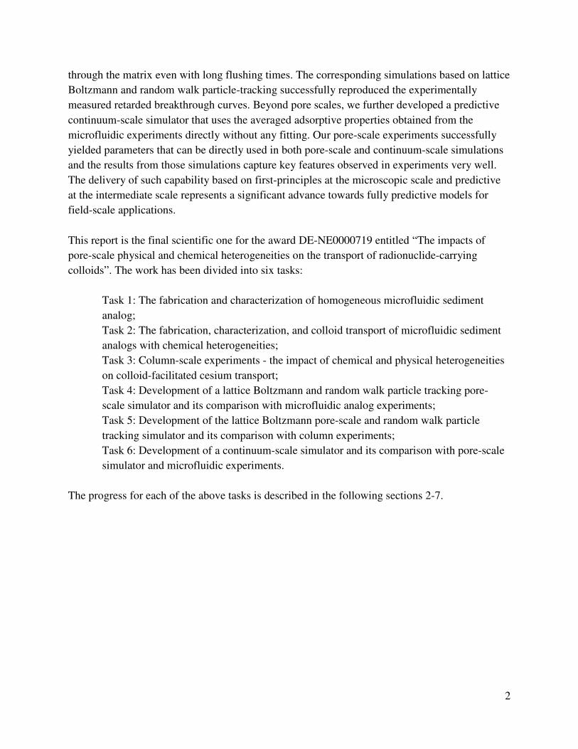
electrostatic interactions with the negatively charged particles (e.g., 1µm and -23mV). Figure 2.8
shows the average fluorescent intensities of retained particles within the carboxylated and
aminated layers. As expected, the positively charged (aminated) beads retained more particles
than the negatively charged (carboxylated) beads in both configurations.
Figure 2.8 Colloids retention in two different types of layered soil analogs. The fluorescent
intensities of particles retained in the soil analog where the carboxylated beads are packed (A)
upstream and (B) downstream. The insets on the top left corner illustrate the analog
configuration .The circles represent the particles accumulated in the aminated bead packing and
the squares are for the carboxylated bead packing. The dash line indicates the moment when we
stopped injecting colloid solution and start to flush with DI water containing no particles.
During the DI water flush some particles detached from the beads, which cause the intensities in
both types of bead packing to decrease first. This indicates that some of the colloidal attachment
in the porous media can be metastable. In Figure 2.8A, where the carboxylated beads were
located upstream, the intensity within the aminated bead packing increased while it decreased in
the carboxylated bead packing. This observation is due to the re-adsorption of particles in the
aminated bead packing that were removed from the carboxylated bead packing. In the opposite

19
configuration (Figure 2.8B), re-adsorption of particles in the downstream carboxylated bead
packing was minimal since the colloid-bead electrostatic interactions are repulsive. As a result,
the fluorescent intensity remains constant at later stage of DI flushing (Figure 2.8B). The
detachment-reattachment of particles observed in certain types of layered soil analogs can have
important implications to colloidal transport in the subsurface environments. First, it would delay
the transport of colloids even in the event of multiple flushing due to the differently charged soil
surfaces. Second, instead of dilution, the flushing could cause the contaminants to concentrate at
locations where colloidal adsorption is energetically favorable. Supplemental video 4 shows the
detachment-reattachment process at certain beads section.
Figure 2.9 The porous soil analog formed by 10 µm aliphatic aminated beads at downstream and
10 µm carboxylated beads at upstream. It shows the opposite configuration as in Figure 2 (B).
The arrow indicates the flow direction of colloids. Scale bar: 200 μm.
2.4 CONCLUSION
We developed a microfluidic bead-based platform that can make soil analogs consisting of
model grains with homogeneous or heterogeneous surface properties. We measured the transport
of both individual and populations of colloidal particles in these soil analogs. Using the pathlines
of individual particles flowing through the pseudo-two-dimensional bead pack, we were able to
extract the tortuosity of differently sized particles and measure the effects of size exclusion and
double layer suppression. The T-junction droplet generator allowed us to measure the transport
of thousands of particles in a single experiment and generate flow-through curves. By

20
demonstrating the capability to make heterogeneous soil analogs in this paper, we expect our
approach can be used in future to study colloidal transport in porous media with different types
of surface heterogeneities (e.g., charge, wettability, and chemical functionality) at the pore scale.
Important insights into the colloid-soil interactions and colloidal transport and retention could
also be obtained by direct comparison of the results obtained from the microscale soil analogs
and larger scale column experiments in future.
This work has been published in Langmuir in 2016. “Bead-Based Microfluidic Sediment
Analogues: Fabrication and Colloid Transport”, Y Guo, J Huang, F Xiao, X Yin, J Chun, W Um,
KB Neeves, N Wu, Langmuir 32 (36), 9342-9350. https://doi.org/10.1021/acs.langmuir.6b02184
The following list of supplementary movies are also published and will be available from the PI
upon request:
SI Video 1: Bead-filling to form the porous soil analog. 15µm polystyrene beads were carried by
fluid flow from the inlet of the device and they became trapped at the height barrier and then
formed the soil analog by packing along the upstream direction.
SI Video 2: Droplets containing colloids moving through an expansion channel. The dark
background in the channel was filled with mineral oil and dye Oil red O. Light green regimes
were the aqueous droplets generated at the T-junction. They encapsulated 1 µm fluorescent
colloids (brighter green dots) that have been flown through the porous medium.
SI Video 3: Individual colloid trajectories. 1.8 × 10⁻⁴ wt% of 1 µm fluorescent PS colloids
solution was used in the experiment. The exposure time was 500 ms to capture the trajectories of
individual colloids.
SI Video 4: Colloids re-mobilization and re-adsorption on the positively charged beads section
placed downstream during flushing.

21
REFERENCES
(1) Tanaka, S.; Nagasaki, S. Impact of Colloid Generation Nn Actinide Migration in High-
Level Radioactive Waste Disposal: Overview and Laboratory Analysis. Nucl. Technol.
1996, 118, 58–68.
(2) Kersting, A. B.; Efurd, D. W.; Finnegan, D. L.; Rokop, D. J.; Smith, D. K.; Thompson, J.
L. Migration of Plutonium in Ground Water at the Nevada Test Site. Nature 1999, 397,
56–59.
(3) Karathanasis, A. D. Subsurface Migration of Copper and Zinc Mediated by Soil Colloids.
Soil Sci. Soc. Am. J. 1999, 63, 830–838.
(4) Kretzschmar, R.; Borkovec, M.; Grolimund, D.; Elimelech, M. Mobile Subsurface
Colloids and Their Role in Contaminant Transport. Adv. Agron. 1999, 66, 121–193.
(5) Roy, S. B.; Dzombak, D. A. Colloid Release and Transport Processes in Natural and
Model Porous Media. Colloids Surfaces A Physicochem. Eng. Asp. 1996, 107, 245–262.
(6) Villholth, K. G. Colloid Characterization and Colloidal Phase Partitioning of Polycyclic
Aromatic Hydrocarbons in Two Creosote-Contaminated Aquifers in Denmark. Environ.
Sci. Technol. 1999, 33, 691–699.
(7) Bradford, S. A.; Yates, S. R.; Bettahar, M.; Simunek, J. Physical Factors Affecting the
Transport and Fate of Colloids in Saturated Porous Media. Water Resour. Res. 2002, 38,
63–1 – 63–12.
(8) Kim, H. N.; Walker, S. L.; Bradford, S. A. Coupled Factors Influencing the Transport and
Retention of Cryptosporidium Parvum Oocysts in Saturated Porous Media. Water Res.
2010, 44, 1213–1223.
(9) Grolimund, D.; Elimelech, M.; Borkovec, M.; Barmettler, K.; Kretzschmar, R.; Sticher, H.
Transport of in Situ Mobilized Colloidal Particles in Packed Soil Columns. Environ. Sci.
Technol. 1998, 32, 3562–3569.
(10) Tufenkji, N.; Redman, J. A.; Elimelech, M. Interpreting Deposition Patterns of Microbial
Particles in Laboratory-Scale Column Experiments. Environ. Sci. Technol. 2003, 37, 616–
623.
(11) Ochiai, N.; Kraft, E. L.; Selker, J. S. Methods for Colloid Transport Visualization in Pore
Networks. Water Resour. Res. 2006, 42, W12S06.
(12) N. K. Karadimitriou and S. M. Hassanizadeh. A Review of Micromodels and Their Use in
Two-Phase Flow Studies. Vadose Zo. J. 2012, 11, 1539–1563.
(13) Song, W.; Kovscek, A. R. Functionalization of Micromodels with Kaolinite for
Investigation of Low Salinity Oil-Recovery Processes. Lab Chip 2015, 15, 3314–3325.
(14) Song, W.; de Haas, T. W.; Fadaei, H.; Sinton, D. Chip-off-the-Old-Rock: The Study of
22
Reservoir-Relevant Geological Processes with Real-Rock Micromodels. Lab Chip 2014,
14, 4382–4390.
(15) Porter, M. L.; Jiménez-Martínez, J.; Martinez, R.; McCulloch, Q.; Carey, J. W.;
Viswanathan, H. S. Geo-Material Microfluidics at Reservoir Conditions for Subsurface
Energy Resource Applications. Lab Chip 2015, 15, 4044–4053.
(16) Lenormand, R.; Zarcone, C. Invasion Percolation in an Etched Network: Measurement of
a Fractal Dimension. Phys. Rev. Lett. 1985, 54, 2226–2229.
(17) Wu, M.; Xiao, F.; Johnson-Paben, R. M.; Retterer, S. T.; Yin, X.; Neeves, K. B. Single-
and Two-Phase Flow in Microfluidic Porous Media Analogs Based on Voronoi
Tessellation. Lab Chip 2012, 12, 253–261.
(18) Kumar Gunda, N. S.; Bera, B.; Karadimitriou, N. K.; Mitra, S. K.; Hassanizadeh, S. M.
Reservoir-on-a-Chip (ROC): A New Paradigm in Reservoir Engineering. Lab Chip 2011,
11, 3785–3792.
(19) Xu, W.; Ok, J. T.; Xiao, F.; Neeves, K. B.; Yin, X.; Xu, W.; Ok, J. T.; Xiao, F.; Neeves,
K. B. Effect of Pore Geometry and Interfacial Tension on Water-Oil Displacement
Efficiency in Oil-Wet Microfluidic Porous Media Analogs Effect of Pore Geometry and
Interfacial Tension on Water-Oil Displacement Efficiency in Oil-Wet Microfluidic
Porous. Phys. Fluids 2014, 26, 093102.
(20) Yadali Jamaloei, B.; Kharrat, R. Fundamental Study of Pore Morphology Effect in Low
Tension Polymer Flooding or Polymer-Assisted Dilute Surfactant Flooding. Transp.
Porous Media 2009, 76, 199–218.
(21) Bowden, S. A.; Cooper, J. M.; Greub, F.; Tambo, D.; Hurst, A. Benchmarking Methods of
Enhanced Heavy Oil Recovery Using a Microscaled Bead-Pack. Lab Chip 2010, 10, 819–
823.
(22) Wu, Q.; Bai, B.; Ma, Y.; Ok, J. T.; Neeves, K. B.; Yin, X. Optic Imaging of Two-Phase-
Flow Behavior in 1D Nanoscale Channels. SPE J. 2014, 19, 793–802.
(23) Wu, Q.; Ok, J. T.; Sun, Y.; Retterer, S. T.; Neeves, K. B.; Yin, X.; Bai, B.; Ma, Y. Optic
Imaging of Single and Two-Phase Pressure-Driven Flows in Nano-Scale Channels. Lab
Chip 2013, 13, 1165–1171.
(24) Corapcioglu, M. Y.; Fedirchuk, P. Glass Bead Micromodel Study of Solute Transport. J.
Contam. Hydrol. 1999, 36, 209–230.
(25) Auset, M.; Keller, A. A. Pore-Scale Processes That Control Dispersion of Colloids in
Saturated Porous Media. Water Resour. Res. 2004, 40, W03503.
(26) Baumann, T.; Werth, C. J. Visualization and Modeling of Polystyrol Colloid Transport in
a Silicon Micromodel. Vadose Zo. J. 2004, 3, 434–443.
(27) Seymour, M. B.; Chen, G.; Su, C.; Li, Y. Transport and Retention of Colloids in Porous

23
Media: Does Shape Really Matter? Environ. Sci. Technol. 2013, 47, 8391–8398.
(28) Wan, J.; Wilson, J. L. Visualization of the Role of the Gas-Water Interface on the Fate and
Transport of Colloids in Porous Media. Water Resour. Res. 1994, 30, 11–23.
(29) Russom, A.; Haasl, S.; Ohlander, A.; Mayr, T.; Brookes, A. J.; Andersson, H.; Stemme,
G. Genotyping by Dynamic Heating of Monolayered Beads on a Microheated Surface.
Electrophoresis 2004, 25, 3712–3719.
(30) Ryan, J. N.; Elimelech, M. Colloid Mobilization and Transport in Groundwater. Colloids
Surfaces A Physicochem. Eng. Asp. 1996, 107, 1–56.
(31) Grumann, M.; Dobmeier, M.; Schippers, P.; Brenner, T.; Kuhn, C.; Fritsche, M.;
Zengerlea, R.; Ducréea, J. Aggregation of Bead-Monolayers in Flat Microfluidic
Chambers Simulation by the Model of Porous Media. Lab Chip 2004, 4, 209–213.
(32) Seong, G. H.; Heo, J.; Crooks, R. M. Measurement of Enzyme Kinetics Using a
Continuous-Flow Microfluidic System. Anal. Chem. 2003, 75, 5206–5212.
(33) Lee, J.; Kim, O.; Jung, J.; Na, K.; Heo, P.; Hyun, J. Simple Fabrication of a Smart
Microarray of Polystyrene Microbeads for Immunoassay. Colloids Surfaces B
Biointerfaces 2009, 72, 173–180.
(34) Xia, Y.; Whitesides, G. M. Soft Lithography. Annu. Rev. Mater. Sci. 1998, 28, 153–184.
(35) Garstecki, P.; Fuerstman, M. J.; Stone, H. A.; Whitesides, G. M. Formation of Droplets
and Bubbles in a Microfluidic T-Junction-Scaling and Mechanism of Break-Up. Lab Chip
2006, 6, 437–446.
(36) van Steijn, V.; Kleijn, C. R.; Kreutzer, M. T. Predictive Model for the Size of Bubbles and
Droplets Created in Microfluidic T-Junctions. Lab Chip 2010, 10, 2513–2518.
(37) Schneider, T.; Burnham, D. R.; VanOrden, J.; Chiu, D. T. Systematic Investigation of
Droplet Generation at T-Junctions. Lab Chip 2011, 11, 2055–2059.
(38) Preibisch, S.; Saalfeld, S.; Tomancak, P. Globally Optimal Stitching of Tiled 3D
Microscopic Image Acquisitions. Bioinformatics 2009, 25, 1463–1465.
(39) Canny, J. A Computational Approach to Edge Detection. IEEE Trans. Pattern Anal.
Mach. Intell. 1986, 8, 679–698.
(40) Montero, R. S.; Bribiesca, E. State of the Art of Compactness and Circularity Measures.
Int. Math. Forum 2009, 4, 1305–1335.
(41) Cornish, R. J. Flow in a Pipe of Rectangular Cross-Section. Proc. R. Soc. A Math. Phys.
Eng. Sci. 1928, 120, 691–700.
(42) Xiao, F.; Yin, X. Geometry Models of Porous Media Based on Voronoi Tessellations and
Their Porosity-Permeability Relations. Comput. Math. with Appl. 2015, 72, 328–348.
(43) D’Humières, D.; Ginzburg, I.; Krafczyk, M.; Lallemand, P.; Luo, L.-S. Multiple-

24
Relaxation-Time Lattice Boltzmann Models in Three Dimensions. Philos. Trans. A. Math.
Phys. Eng. Sci. 2002, 360, 437–451.
(44) Zou, Q.; He, X. On Pressure and Velocity Flow Boundary Conditions and Bounceback for
the Lattice Boltzmann BGK Model. Phys. Fluids 1997, 9, 1591–1598.
(45) Maier, R. S.; Kroll, D. M.; Bernard, R. S.; Howington, S. E.; Peters, J. F.; Davis, H. T.
Pore-Scale Simulation of Dispersion. Phys. Fluids 2000, 12, 2065–2079.
(46) Salles, J.; Thovert, J.-F.; Delannay, R.; Prevors, L.; Auriault, J.-L.; Adler, P. M. Taylor
Dispersion in Porous Media. Determination of the Dispersion Tensor. Phys. Fluids A
Fluid Dyn. 1993, 5, 2348–2376.
(47) Verruijt, A. Soil Mechanics, 1st ed.; Delft University of Technology, 2004.
(48) Carman, P. C. Fluid Flow through Granular Beds. Chem. Eng. Res. Des. 1997, 75, S32–
S48.
(49) Pace, M. N.; Mayes, M. A.; Jardine, P. M.; Mehlhorn, T. L.; Zachara, J. M.; Bjornstad, B.
N. Quantifying the Effects of Small-Scale Heterogeneities on Flow and Transport in
Undisturbed Core from the Hanford Formation. Vadose Zo. J. 2005, 4, 1220–1223.

25
3. Task 2: The fabrication, characterization, and colloid transport of
microfluidic sediment analogs with chemical heterogeneities
3.1 INTRODUCTION
Engineered and natural colloidal particles typically have a size range of a few nanometers to
several microns.1 In the subsurface environment, there are usually three types of particles:
inorganic, organic, and biocolloids. Due to their relatively small sizes, when they are released
into the environment, they can easily find their paths through the porous subsurface and enter the
ground water flow. These particles endanger aquifers in two aspects. On one hand, they can pose
a threat to the health of living creatures including human beings. For example, Ahmed et al2
found graphene oxide particles cause a significant reduction in microbial metabolic activities. In
1993, there was an outbreak of cryptosporidium infection transmitted through the public water
supply in Milwaukee that affected around 400,000 people locally.3 On the other hand, the
particles also act as carriers for otherwise insoluble contaminants such as radionuclides, heavy
metals, or organic substances, which adsorb on colloidal particles and travel over a much longer
distance than themselves alone.4 Therefore, it is important to understand the transport
mechanisms of colloidal particles in porous media.
Traditionally, laboratory-scale experiments on colloidal transport are performed through columns
of tens of centimeters in length and several centimeters in diameter. Inside the column, model or
real soil grains are packed as porous medium and colloidal suspension are injected from one end
of the column. The breakthrough curves are then measured at the other end. In this method, the
physical heterogeneity of the porous medium such as grain size distribution can be controlled by
mixing two or more types of sand beads of different sizes. In contrast, the studies on porous
media with chemical heterogeneities are scarce. Only a few works have been reported and the
conclusions are somewhat contradictory. For example, Chen et al5 modified sand grains with
aminosilane molecules so that they bear positive surface charges. They then packed the column
with two types of sand grains with opposite surface charges to form a heterogeneous porous
medium. They found that the overall collector and collision efficiencies primarily follow a linear
relation with respect to the percentage of grains that are favorable for particle deposition.
However, Abudalo et al6 found a different relationship for different microorganisms. In their
study the collision efficiency of Cryptosporidium parvum oocysts is two times proportional to
the ratio of favorable deposition sand grains.
Apart from the inconsistence mentioned above, another discrepancy reported from the literature
is the colloidal deposition coefficient k. According to the classic filtration theory, k is a constant
and can be obtained by fitting either the breakthrough curve or the retention profile of particles in
the porous medium. However, the results obtained from these two methods usually do not
match.7,8 To solve this issue, Tufenkji et al,8,9 proposed that k can be a function rather than a

26
constant. Although a number of distribution functions have been proposed, it is unclear whether
there exists a universal one that can apply to a wide range of data in general.
Previous work has primarily focused on physical heterogeneities due to the lack of experimental
models with tunable chemical heterogeneities at the pore-scale. Here, we developed a
microfluidic fabrication method that are capable to make chemically heterogeneous porous
media by assembling colloidal particles with opposite surface charges. Meanwhile, this method
allows us to accurately determine the breakthrough curve and retention profiles of particles. With
our experimental setup we are able to observe the dynamics of colloid deposition at pore-scale
and in real time. With the assistance of this new device we aim to obtain measurable deposition
coefficient that can be directly used in both pore-scale and continuum-scale simulations.
3.2 MATERIALS AND METHODS
Materials
Polydimethylsioxane (PDMS) was purchased from Dow Corning (Sylgard 184, Midland, MI).
1H-1H-2H-2H-perfluorooctyltrichlorosilane was bought from Gelest (Morrisville PA).
Photoresist (KMPR1010 and KMPR1050) came from MicroChem (Newton, MA). Photoresist
developer (AZ300 MIF) was from AZ Electronic Materials (Somerville, NJ). 0.5 µm (diameter)
carboxylated red (580/605 nm) polystyrene (PS) colloidal particles was purchased from Life
Technologies (Carlsbad, CA), 10 µm (dimeter) blue (360/407 nm) fluorescent PS microspheres
was purchased from Polysciences, Inc. (Warrington, PA) and 10 µm amino-polystyrene particles
were purchased from Spherotech, Inc. (Lake Forest, IL). Three-inch silicon wafers were from
Silicon Inc. (Boise, ID). Gauge 30 Tygon tubing was from Saint-Gobain North America (ID =
0.01″, OD = 0.03″, Valley Forge, PA). Biopsy punch (0.75 mm) was from World Precision
Instrument (Sarasota, FL). Microfluidic valve (MV202) was purchased from LabSmith, Inc.
(Livermore, CA).
Device fabrication
The microfluidic devices were fabricated with PDMS using standard soft lithography
techniques10 while the master wafer was made by a two-step photolithography procedure. The
detailed procedures have been described in our previous work,11 except that we used 8,000 rpm
for 40 seconds to obtain a 8 µm thick photoresist layer during the spin coating of the first layer.
Identification of the location of different types of beads
We used a similar particle tracking method as Guo et al11 to identify the location of individual
beads in the fabricated porous media. We used a confocal microscope (Olympus Fluoview i10)
with a 60x objective for imaging. Therefore the threshold in the MATLAB script is different: the
first filtration cutoff for the circumference is between 10 and 51 μm, and the second filtration cut
off for area is between 4.3 and 25.7 μm2, while the rest of the thresholds remain the same as in

27
our previous paper.11 In addition to the x-y position of the mass center of each bead, we also need
to distinguish both positively and negatively charged beads. Since the negatively charged beads
are labeled with blue fluorophore while the positively charged beads are not, only negatively
charged beads will be revealed under fluorescent microscopy. When we overlay the fluorescent
image with the bright field image, those negatively charged beads are all saturated with white
pixel so that we can identify the sign of surface charges on each bead. The z-position of the mass
center of each bead can also be obtained by accurately scanning the porous media from the
bottom to top using the confocal microscopy.
Breakthrough curve and retention profile
Breakthrough curves were obtained by recording the colloidal nanoparticles in the channel right
before they entered and immediately after they exited the porous medium. We used an automated
stage so that optical images were taken at those two locations alternatively with a two-second
time interval. After the flow experiments, images were analyzed with a customized MATLAB
script. The script used bwareaopen command to filter out noises and bwboundaries command to
trace the exterior boundaries of each particle trajectory. The summation of bwboundaries returns
the total number of particles in the image view. Since the volume of the channel captured in the
image is know from design, we are able to obtain the colloidal concentration at both locations for
a function of time. The retention profile of colloidal nanoparticles was obtained along with the
bead location imaging via the confocal microscopy. The particles are labeled with TRITC
fluorophore so they can be easily distinguished from the background porous medium. The laser
intensity is set to be 40% and its sensitivity is 3%. The scanning interval along the z-direction is
set to be 2 μm to minimize the signal noises coming from other focal planes. For aggregated
particles that are deposited in the porous medium, we use the bwboundaries command in our
MATLAB script to trace the perimeter of each particles. A threshold of 40 pixels was adopted to
separate individual particles from aggregate. Below that threshold, all particles were treated as
counted as single deposition, above which the number of particles in the clusters was determined
by rounding up the ratio of cluster’s area to the threshold value. The position of each deposited
particle was also recorded for the analysis of retention profiles.
Pore-scale experiments
In the pore-scale experiments, a 60X oil-immersion objective on Olympus IX81 was used to
record the dynamics of colloidal deposition at a fixed bead location for one hour with a time of
interval of one second. After recording the dynamics, the porous medium was placed under a
confocal microscope with 120X magnification for an accurate three-dimensional (3D) mapping
of the deposited colloids.
Calculation of the effective range of the double-layer interactions between colloidal
nanoparticles and beads

28
The double-layer interaction between colloidal nanoparticles and bead collectors is determined
from Sader et al,21
( ) ( ) ( ) ( )2
2 21 21 2 1 2ln 1 ln 1
4
h ha akTU y y e y y e
e R
κ κε − − = + + + − − (3.1)
where a1 (5 µm) and a2 (250 nm) are radii of an amine-functionalized bead and the carboxylated
nanoparticles, R is the distance between the centers of two spheres, y1 and y2 are the reduced
surface potentials and we approximate them with measured zeta potentials here. h is the surface
to surface distance between two spheres and κ-1 is the Debye length.15 Although we used DI
water in our experiments, dissolved carbon dioxide (CO2) from air will generate H+ and 3HCO−
ions in solution. The concentration of H+ can be inferred by measuring pH of the DI water,
which is between 5.5 to 6.0, in agreement with data provided by Ropp.16 Correspondingly, the
concentration of 3HCO− is 2.23×10⁻⁶ M, which yields a Debye length of 205 nm. This value,
however, is on the higher end of the Debye length reported from varies sources,17–19 since ion
leakage from both glassware and particle surfaces will further reduce the Debye length. Here, we
adopted the value from Kampf et al,20 which gives a Debye length of 68 nm. From Eq. (1), we
are able to calculate the interaction energy normalized by thermal energy kT as a function of
surface-to-surface separation (h) normalized by the Debye length, as shown in the
Supplementary Figure 3.1. We assume that when U~10 kT, the nanoparticles will be 100%
deposited on the collector, which corresponds to a surface-to-surface separation of 272 nm. After
taking the nanoparticle radius (250 nm) into account, the distance for nanoparticles to adsorb on
beads in pore-scale simulations is set to be 520 nm.
3.3 RESULTS AND DISCUSSION
Fabrication and characterization of chemically heterogeneous porous media
To fabricated heterogeneous porous media, we need to inject suspension of both positively and
negatively charged beads into the microfluidic device. The oppositely charged beads, however,
will quickly aggregate with each other in solution. If we introduce them into separate streams,
the amine-functionalized beads will also deposit on the microfluidic channel wall before even
reaching the packing chamber since the wall is typically negatively charged. To solve this issue,
we mix the carboxyl- and amine-functionalized beads in 0.01 M NaOH solution. Although the
amine-beads exhibit a positive zeta potential (ζ = 59±1 mV) at pH 7, they bear negative charges
(ζ = -92±2 mV) in pH 12. This change of surface charges allows us to inject the mixture into the
microfluidic chamber without problems of deposition or aggregation. After the porous medium is
fabricated, we flow DI water thoroughly (20 nL/s for 30 minutes) to restore the positive surface
charges on the amine-functionalized beads, where an ex-situ experiment shows that the zeta
potential recovers to 68±4 mV.
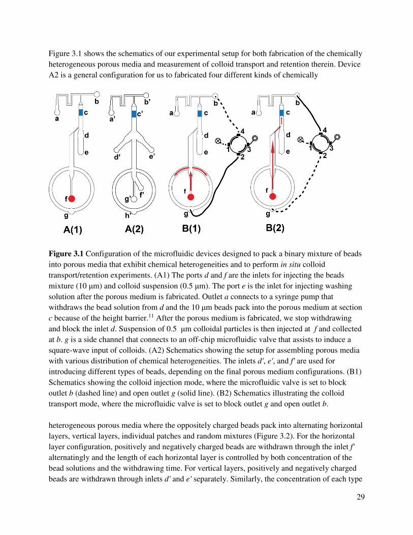
29
Figure 3.1 shows the schematics of our experimental setup for both fabrication of the chemically
heterogeneous porous media and measurement of colloid transport and retention therein. Device
A2 is a general configuration for us to fabricated four different kinds of chemically
Figure 3.1 Configuration of the microfluidic devices designed to pack a binary mixture of beads
into porous media that exhibit chemical heterogeneities and to perform in situ colloid
transport/retention experiments. (A1) The ports d and f are the inlets for injecting the beads
mixture (10 μm) and colloid suspension (0.5 μm). The port e is the inlet for injecting washing
solution after the porous medium is fabricated. Outlet a connects to a syringe pump that
withdraws the bead solution from d and the 10 μm beads pack into the porous medium at section
c because of the height barrier.11 After the porous medium is fabricated, we stop withdrawing
and block the inlet d. Suspension of 0.5 μm colloidal particles is then injected at f and collected
at b. g is a side channel that connects to an off-chip microfluidic valve that assists to induce a
square-wave input of colloids. (A2) Schematics showing the setup for assembling porous media
with various distribution of chemical heterogeneities. The inlets d', e', and f' are used for
introducing different types of beads, depending on the final porous medium configurations. (B1)
Schematics showing the colloid injection mode, where the microfluidic valve is set to block
outlet b (dashed line) and open outlet g (solid line). (B2) Schematics illustrating the colloid
transport mode, where the microfluidic valve is set to block outlet g and open outlet b.
heterogeneous porous media where the oppositely charged beads pack into alternating horizontal
layers, vertical layers, individual patches and random mixtures (Figure 3.2). For the horizontal
layer configuration, positively and negatively charged beads are withdrawn through the inlet f'
alternatingly and the length of each horizontal layer is controlled by both concentration of the
bead solutions and the withdrawing time. For vertical layers, positively and negatively charged
beads are withdrawn through inlets d' and e' separately. Similarly, the concentration of each type
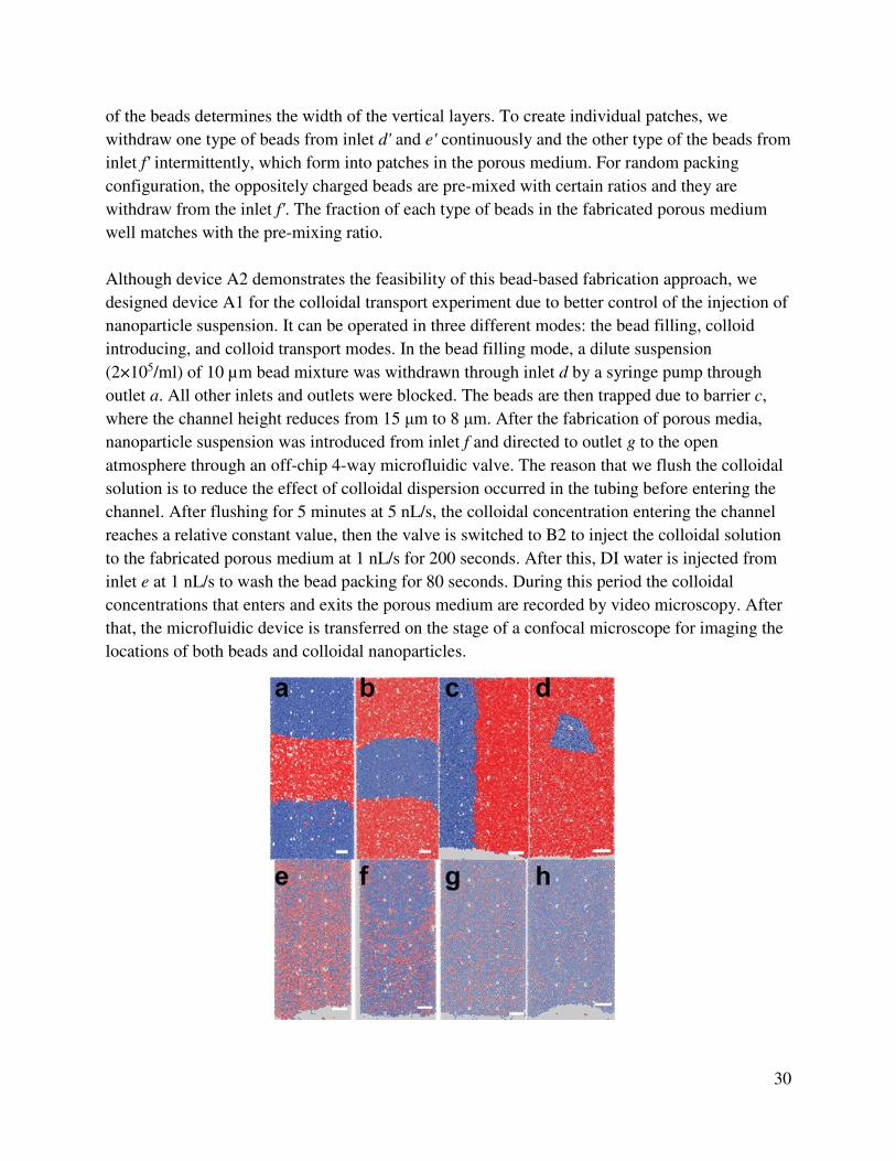
30
of the beads determines the width of the vertical layers. To create individual patches, we
withdraw one type of beads from inlet d' and e' continuously and the other type of the beads from
inlet f' intermittently, which form into patches in the porous medium. For random packing
configuration, the oppositely charged beads are pre-mixed with certain ratios and they are
withdraw from the inlet f'. The fraction of each type of beads in the fabricated porous medium
well matches with the pre-mixing ratio.
Although device A2 demonstrates the feasibility of this bead-based fabrication approach, we
designed device A1 for the colloidal transport experiment due to better control of the injection of
nanoparticle suspension. It can be operated in three different modes: the bead filling, colloid
introducing, and colloid transport modes. In the bead filling mode, a dilute suspension
(2×10⁵/ml) of 10 µm bead mixture was withdrawn through inlet d by a syringe pump through
outlet a. All other inlets and outlets were blocked. The beads are then trapped due to barrier c,
where the channel height reduces from 15 μm to 8 μm. After the fabrication of porous media,
nanoparticle suspension was introduced from inlet f and directed to outlet g to the open
atmosphere through an off-chip 4-way microfluidic valve. The reason that we flush the colloidal
solution is to reduce the effect of colloidal dispersion occurred in the tubing before entering the
channel. After flushing for 5 minutes at 5 nL/s, the colloidal concentration entering the channel
reaches a relative constant value, then the valve is switched to B2 to inject the colloidal solution
to the fabricated porous medium at 1 nL/s for 200 seconds. After this, DI water is injected from
inlet e at 1 nL/s to wash the bead packing for 80 seconds. During this period the colloidal
concentrations that enters and exits the porous medium are recorded by video microscopy. After
that, the microfluidic device is transferred on the stage of a confocal microscope for imaging the
locations of both beads and colloidal nanoparticles.

31
Figure 3.2 Different configurations of chemical heterogeneity in the fabricated porous media
packed by a binary mixture of oppositely charged beads. (a) and (b) Alternating horizontal
layers, (c) Vertical layers, and (d) single patches, (e)-(h): random mixing with 48%, 24%, 9%,
and 4% positively charged beads, respectively. The red spheres represent beads functionalized
with amine (positively charged) and blue ones are for carboxyl-functionalized beads (negatively
charged). Scale bars: 100 μm.
Figure 3.3 Radial distribution functions ( )g r for different bead pairs in a porous medium
randomly packed by 48% positively and 52% negatively charged beads. The dots are from
experimental measurement and solid lines are predictions from numerical simulations.

32
Figure 3.2 shows different configurations of the charge heterogeneity that we can make with
device A2 in Figure 3.1. Figures 3.2a-d demonstrate our ability to assemble oppositely charged
beads into alternating horizontal layers, vertical layers, and individual patches, where the blue
spheres represent carboxyl-functionalized beads and the red ones are beads with amines. Figures
3.2e-h show the porous media that are randomly packed by the binary mixture with different
fractions of the amine-functionalized beads. To quantify the degree of randomness in bead
packing, we measured the radial distribution functions ( )ij
g r for different bead pairs.
Figure 3.3 displays ( )ij
g r for different bead pairs measured from the porous medium shown in
Figure 3.2e, i.e., the one packed by 48% amine-functionalized beads and 52% carboxyl-
functionalized beads randomly. We also performed numerical simulations, in which the beads’
locations and number densities are the same as in experiments but the bead type is randomly
assigned between amine- and carboxyl-beads via a random number generator. Clearly, for each
type of bead pairs, the experiment data agree with the simulation results very well, which
suggests that the distribution of these two types of beads are indeed random. The R2 values
shown in Table 3.1 for this case are all above 0.94, indicating that the difference between
experiments and simulations are marginal. The Supplementary Figure 3.1 show ( )ij
g r measured
from Figure 3.2f-h. For the amine-carboxyl pair, the radial distribution function becomes more
and more sensitive to the location of the amine-beads as its fraction decreases. Therefore, for
lower fractions, R2 obtained from the carboxyl–amine bead pair is a better reflection of the
degree of randomness. Here, even for 4% mixture, the R2 value is still above 0.9, indicating the
uniform distribution of the amine-functionalized beads.
Table 3.1 R2 values for each type of bead pairs in the comparison of radial distribution functions
between experiments and simulation
fraction of amine-functionalized beads carboxyl-carboxyl amine-amine carboxyl-amine
48% 0.9668 0.9477 0.9925
24% 0.9846 0.8074 0.8969
17% 0.9946 0.7968 0.9767
9% 0.9983 0.6717 0.9327
4% 0.9998 0.4104 0.9590
Measurement of the breakthrough curves
To obtain a breakthrough curve that reflects the real dynamics of colloid transport through a
porous medium, we need to generate a sharp front during injection of colloidal suspension.
However, in a microfluidic device, the dispersion of colloidal flow can occur within the tubing

33
way before it enters the channel, which will largely smear the concentration front. To solve this
problem, we used an off-chip 4-way microfluidic valve that was connected to a cross channel at
the upstream of the fabricated porous medium. After flushing with DI water for 30 minutes, the
colloidal suspension entering the device was first directed to outlet g through the circular side
channels as illustrated in Figure 3.1-B1 to completely eliminate the influence of dispersion. After
the concentration of the incoming colloids reaches a steady state, the 4-way valve is turned 90º
clockwise to connect outlet b to the cross channel and block the outlet g. The colloidal
suspension can then be directed to flow through the porous medium. Supplementary Figure 3.2
demonstrates the distinct difference of the colloid injection input at the entrance of the porous
medium with and without this specific valve design. Equipped with the valve, the particle
concentration exhibits a rapid rise and reaches steady state within 4 pore volume (PV), in
contrast, the one without valve shows a gradual increment in concentration which does not reach
steady state even after 30 PV. Therefore, we implemented this valve design in all experiments.
Figure 3.4 shows the breakthrough curves of 0.5 μm carboxylated PS nanoparticles flowing
through chemically heterogeneous porous media that are randomly packed by oppositely charged
beads with different number ratios. Since little particle deposition is observed on the chemically
homogeneous porous medium that is packed by negatively charged beads only, its breakthrough
curve reaches the plateau of / 1out inC C = around 5 PV. In comparison, the presence of positively
charged beads, even with a small fraction of 4% and 9%, delays the onset of plateau to around 8
PV. With higher fractions, no clear plateau can be observed. Instead, the outlet concentration
increases gradually, followed by quick decline during the DI water flushing period. We attribute
this phenomenon to the Langmuir effect that sites available for nanoparticle deposition on the
amine-beads are limited. Since the electrostatic interaction between the carboxyl-functionalized
beads and nanoparticles are repulsive, particle deposition and retention primarily occurred on the
amine-beads. For these electrostatically attractive beads, the early incoming colloids can easily
occupy many of the available sites. However, there will be less chance for colloids to deposit
later. Therefore, as time increases more colloids will come out of the porous medium. Another
phenomenon we observed is that a very small fraction of the positively charged beads changes
the breakthrough curve dramatically. 4% amine-beads present in the porous medium reduces the
breakthrough curve plateau from 100% to 60%, and 9% amine-beads further reduces it to 30%.
When the fraction of amine-beads reaches 25%, nanoparticles barely pass through the porous
medium. This observation agrees qualitatively with results from column experiments published
previously.13 But the degree of plateau value reduction is, however, different for the same
fraction of positively charged beads, which could be attributed to the zeta potential difference
between our packed polystyrene beads and their iron oxyhydroxide coated quartz granules.

34
Figure 3.4 Breakthrough curves for the transport of 0.5 µm caboxylated nanoparticles in
chemically heterogeneous porous media packed by a random mixture of amine- and carboxyl-
functionalized beads with different fractions.
Colloid retention profile
After the breakthrough experiments, the microfluidic device was disconnected from syringe
pumps and valves and transferred to a confocal microscope for mapping out the colloid retention
profiles. The entire porous medium was scanned using a 60X water emersion objective both
laterally and vertically. For each lateral scan, z-stacks with 1 μm interval were performed to
obtain three-dimensional locations of all colloids deposited based on an image processing
program. We further identified the beads where those nanoparticles were deposited on, based on
the bead-nanoparticle separation.
Figure 3.5a shows the number of deposited nanoparticles as a function of distance along the
porous medium. It can be seen that most particles were adsorbed at the upstream. The colloid
concentration was greatly reduced beyond first few hundred microns. Figure 3.5a shows that the
higher the fraction of amine-beads, the steeper the slope is, as these beads are effective collectors
for retaining a significant fraction of mobile nanoparticles. The slopes of lines in Figure 3.5a
correspond to the ratio of the overall deposition coefficient k and the interstitial particle velocity
vp. Figure 3.5b plots k (normalized by k0, which is the deposition coefficient for a porous
medium packed by amine-beads only) for different cases. Clearly, k is proportional to the
fraction of the positively charged beads, i.e., k = fk0. This linear relationship is expected for a
binary system where the extent of unfavorable deposition is negligible.

35
Figure 3.5 (a) The retention profiles for 0.5 μm carboxylated nanoparticles in chemically
heterogeneous porous media packed by a random mixture of amine- and carboxyl-functionalized
beads with different fractions. (b) The normalized overall deposition coefficient k/ko as a
function of the fraction of amine-beads present in the porous media.
Pore-scale experiments
One unique advantage of our approach is that we are able to capture the pore-scale dynamic
process of colloidal deposition in situ, which is shown in the supplementary video 1. Each black
ring shown in the video represents a bead captured in the bright field. The focal plane was
chosen near the bead equator (around 7 µm above the bottom of the substrate) for accurate
detection of the bead centers. The bright dots are 0.5 µm carboxylated PS nanoparticles. For
beads located at the bottom layer, the retained colloids are obscured by the equator and thus a
ring surrounding the bead appears because of light scattering. From the video, most nanoparticles
were adsorbed on the amine-functionalized beads because of the electrostatic attraction. But
among those amine-beads, different rates of deposition were observed possibly due to variability
in surface potentials among them. In addition, a few nanoparticles were also deposited on the
carboxyl-functionalized beads due to either straining or secondary minimum interaction.9

36
Figure 3.6 The evolution of surface coverage on five isolated amine-functionalized beads.
Dashed lines are the least square fitting following the theory.
Figure 3.7 Nanoparticles deposited on one isolated amine-functionalized bead. (a)-(f) confocal
microscopy images scanned from the bottom of the bead to its equator with 1 μm step change.
(g) digital reconstruction of the deposited nanoparticles for a half hemisphere. The flow direction
of particles is from bottom to top.
Figure 3.6 shows the temporal change of the surface coverage on five different amine-beads. The
surface coverage increases fast initially and can be approximated by a linear relationship at the
first 200 seconds. Afterwards it slowed down and flattened out. This clearly demonstrates a
surface-blocking phenomenon and the early deposited particles hinder the deposition of latter
particles. We can fit the experimental data in Figure 3.6 and obtain the deposition coefficient
kpore, which matches the random sequential adsorption theory very well. It is also worth noting
that nanoparticle deposition first occurred on the front hemisphere of amine-beads. After the
adsorption sites were largely filled, the deposition progressively moved to the rear hemisphere.

37
Figure 3.7 displays the deposited nanoparticles on an isolated amine-bead after one-hour
experiment. It is clear that more particles were deposited on the front hemisphere than the rear
one because of the shape of streamlines. Another observation worth mentioning is that at the
front hemisphere, local particle concentration is higher than the rear. This also demonstrates that
the previously deposited particles intercepted the latter ones primarily in the front hemisphere.
The area that is free of particle at the bottom left corner is because of the presence of another
bead in the packing, which physically blocked the space and prevented particles from adsorbing.
3.4 CONCLUSION
We developed a microfluidic bead-based fabrication method that are capable to make
heterogeneous porous media by assembling colloidal particles with opposite surface charges so
that the chemical heterogeneities can be precisely defined at the length scale of a single grain.
We demonstrated our ability to make four different configurations of chemical heterogeneities:
the alternating horizontal layers, vertical layers, single patches, and random mixing. We further
characterized the spatial distribution of pore-scale heterogeneities, measured the in situ transport
and retention of colloids in the fabricated porous media using bring-field, fluorescence, and
confocal microscopy at the resolution less than 1 µm. We found that a very small fraction of the
positively charged beads present in the porous medium changes the breakthrough curve
dramatically. The overall deposition coefficient k measured from the colloid retention curves is
proportional to the fraction of the positively charged beads as the extent of unfavorable
deposition is negligible. For the first time, we measured the pore-scale dynamic process of
colloidal deposition in situ. The measured deposition coefficient at the pore-scale, i.e., kpore
matches the random sequential adsorption theory very well.

38
Supplementary Figure 3.1 Radial distribution functions ( )g r for different bead pairs in porous
media that are randomly packed by different fraction of positively and negatively charged beads.
The dots are experimental measurement and solid lines are from numerical simulations.
Supplementary Figure 3.2 The concentration profile of injected nanoparticles at the entrance of
the porous medium with and without special valve design.

39
REFERENCE
(1) Ryan, J. N.; Elimelech, M. Colloid Mobilization and Transport in Groundwater. Colloids
Surfaces A Physicochem. Eng. Asp. 1996, 107, 1–56.
(2) Ahmed, F.; Rodrigues, D. F. Investigation of Acute Effects of Graphene Oxide on
Wastewater Microbial Community: A Case Study. J. Hazard. Mater. 2013, 256–257
(Supplement C), 33–39.
(3) MacKenzie, W. R. A Massive Outbreak in Milwaukee of Cryptosporidium Infection
Transmitted Through the Public Water Supply. N. Engl. J. Med. 1994, 331 (3), 161–167.
(4) McCarthy, J.; Zachara, J. Subsurface Transport of Contaminants. Environ. Sci. Technol.
1989, 23 (5), 496–502.
(5) Chen, J. Y.; Ko, C. H.; Bhattacharjee, S.; Elimelech, M. Role of Spatial Distribution of
Porous Medium Surface Charge Heterogeneity in Colloid Transport. Colloids Surfaces A
Physicochem. Eng. Asp. 2001, 191 (1–2), 3–15.
(6) Abudalo, R. A.; Bogatsu, Y. G.; Ryan, J. N.; Harvey, R. W.; Metge, D. W.; Elimelech, M.
Effect of Ferric Oxyhydroxide Grain Coatings on the Transport of Bacteriophage PRD1
and Cryptosporidium Parvum Oocysts in Saturated Porous Media. Environ. Sci. Technol.
2005, 39 (17), 6412–6419.
(7) Tufenkji, N.; Elimelech, M. Deviation from Colloid Filtration Theory in the Presence of
Repulsive Electrostatic Interactions: Implications to Microbial Transport. 2004, No. 21,
ENVR-095.
(8) Tufenkji, N.; Redman, J. A.; Elimelech, M. Interpreting Deposition Patterns of Microbial
Particles in Laboratory-Scale Column Experiments. Environ. Sci. Technol. 2003, 37, 616–
623.
(9) Tufenkji, N.; Elimelech, M. Breakdown of Colloid Filtration Theory : Role of the
Secondary Energy Minimum and Surface Charge Heterogeneities. Langmuir 2005, No.
1821, 841–852.
(10) Xia, Y.; Whitesides, G. M. Soft Lithography. Annu. Rev. Mater. Sci. 1998, 28, 153–184.
(11) Guo, Y.; Huang, J.; Xiao, F.; Yin, X.; Chun, J.; Um, W.; Neeves, K. B.; Wu, N. Bead-
Based Microfluidic Sediment Analogues: Fabrication and Colloid Transport. Langmuir
2016, 32, 9342–9350.
(12) Johnson, P. R.; Elimelech, M. Dynamics of Colloid Deposition in Porous Media :
Blocking Based on Random Sequential Adsorption. Langmuir 1995, 11, 801–812.
(13) Johnson, P. R.; Sun, N.; Elimelech, M. Colloid Transport in Geochemically
Heterogeneous Porous Media : Modeling and Measurements. Environ. Sci. Technol. 1996,
30, 3284–3293.
(14) Kretzschmar, R.; Barmettler, K.; Grolimund, D.; Yan, Y.; Borkovec, M.; Sticher, H.
Experimental Determination of Colloid Deposition Rates and Collision Efficiencies in
Natural Porous Media. Water Resour. Res. 1997, 33 (5), 1129–1137.
(15) Israelachvili, J. Intermolecular and Surface Forces; 2011.

40
(16) Ropp, R. C. Encyclopedia of the Alkaline Earth Compounds; 2013.
(17) Wu, H. J.; Pangburn, T. O.; Beckham, R. E.; Bevan, M. A. Measurement and
Interpretation of Particle-Particle and Particle-Wall Interactions in Levitated Colloidal
Ensembles. Langmuir 2005, 21 (22), 9879–9888.
(18) Rupp, B.; Torres-Díaz, I.; Hua, X.; Bevan, M. A. Measurement of Anisotropic Particle
Interactions with Nonuniform Ac Electric Fields. Langmuir 2018, 34 (7), 2497–2504.
(19) Ghosal, S. Mathematical Modeling of Electrokinetic Effects in Micro and Nano Fluidics.
In Microfluidics and Microfabrication; 2010; pp 87–112.
(20) Kampf, N.; Ben-Yaakov, D.; Andelman, D.; Safran, S. A.; Klein, J. Direct Measurement
of Sub-Debye-Length Attraction between Oppositely Charged Surfaces. Phys. Rev. Lett.
2009, 103 (11), 1–4.
(21) Sader, J. E.; Carnie, J. L.; Chan, D. Y. C. Accurate Analytic Formulas for the Double-
Layer Interaction between Spheres. J. Colloid Interface Sci. 1995, No. 171, 46–54.
(22) Schaaf, P.; Talbot, J. Surface Exclusion Effects in Adsorption Processes. J. Chem. Phys.
1989, 91 (7), 4401–4409.
(23) Adamczyk, Z.; Belouschek, P. Localized Adsorption of Particles on Spherical and
Cylindrical Interfaces. J. Colloid Interface Sci. 1991, 146 (1), 123–136.
(24) Johnson, P. R.; Elimelech, M. Dynamics of Colloid Deposition in Porous Media: Blocking
Based on Random Sequential Adsorption. Langmuir 1995, 11 (3), 801–812.

41
4. Task 3: Column-scale experiments: The impact of chemical and
physical heterogeneities on colloid-facilitated cesium transport
4.1 INTRODUCTION
Mobility of contaminants in the subsurface is known to be facilitated by colloids transported with
groundwater1-4 while contaminants strongly adsorb on the surface of colloids. This is a concern
as it can lead to more and faster spreading of contamination than conventional model prediction
in environmentally sensitive waters. Contaminants of interest can form strong bonds with silicate
materials, including colloids, and be transported to environmentally sensitive systems. These
contaminants include radionuclides such as cesium (137Cs) which have been released to the
environment at several DOE sites.5, 6 Much research has focused on colloid facilitated transport
of Cs with significant interest on the influence of interfacial phenomena including unsaturated
transport and transport through complex natural sediments.5, 7-11
For example, at the Hanford site in Richland Washington, Cs has contaminated the subsurface
from leaking underground storage tanks spilling high ionic strength radioactive leachate. As the
leachate wets the initially dry vadose zone sediment it mobilizes colloids and can contain 137Cs.12
Though with decreasing pore velocity and decreasing ionic strength as leachate reacts with
surrounding media and mixes with more dilute groundwater Cs can be stripped off of colloids
onto the stationary sediment.12 Chemical and physical heterogeneities found in natural sediment
can further retard Cs transport especially at locations with certain minerals such as mica, on
which Cs will form a strong chemical bond to edge sites.6
It has been shown that slight changes in chemical and physical fabric of natural sediment and
sand can have profound influence on transport of colloids.13, 14 At interfaces within the sediment
pores the colloids will transport into a new pore network where they will more likely move
through or into smaller pores or dead end pores15 and can then be strained reducing transport.16
The straining can be further exasperated by colloids “bridging” between grains in pores.16 Subtle
changes in surface characteristic of the sediment or colloid will also change the transport of
colloids. When chemical heterogeneities such as natural organic matter in sediment or on colloid
surfaces exist, the transport of colloids increase compared to mineral surfaces free of organic
matter due to the increased complexities on the surface.4, 13 However, if the organic material
makes the sediment’s surface hydrophobic the transport of hydrophilic colloids can be slowed or
stopped in the porous matrix.17
Often studies simplify the colloid systems to better understand the effects of heterogeneities on
colloid transport and colloid facilitated transport by using columns packed with quartz sand14, 15,
however, sand matrix such as this have heterogeneities on their surfaces and the influence of
subtle differences of heterogeneities can be obscured. A more controlled transport environment

42
involves colloid transport through micro-fluidic devices with an etched matrix18, 19, these
matrices are designed to be effectively two dimensional and do not have natural channel
narrowing where colloid bridging occurs. To produce a microfluidic environment which can be,
in some capacity, replicated in a column environment Guo, et al. 20 performed a colloid transport
experiment using a matrix of beads rather than having a fabricated porous matrix. Such an
experimental design allows for comparisons with column research when similar matrix
geometries are scaled to the larger condition.
The objectives of this research are: 1) to investigate the influence of physical heterogeneities on
the fate of Cs and colloids through a porous media subjected to low pore velocity, 2) to
investigate the influence of hydrophobic/hydrophilic chemical heterogeneity on transport of Cs
and colloids, 3) to compare our results to microfluidic experiments performed with similar
conditions. Using 1-µm SiO2 colloids and CsI spiked solution we investigated the influence of
colloid-facilitated Cs transport under relevant physicochemical porous media conditions in
columns packed with glass beads.
4.2 MATERIALS AND METHODS
Materials
The solution used for column experiments was deionized water spiked with CsI to 0.5 mM11 and
1-µm colloids (SiO2 microspheres; Corpuscular Co. Cold Spring NY) were added to a
concentration of 50 mg L-1, an observed concentration from Hanford sediments21. The colloids
were received from the manufacturer suspended in a brine solution with a pH >8.0. Before
adding the colloids to the experimental solution the colloid suspension was washed repeatedly
with deionized water until the remaining colloid suspension in water became pH 6.1, which was
the same pH as 0.5 mM CsI in deionized water. This was achieved by centrifugation of the
colloids in brine solution then removing the solution with pipette and replacing with deionized
water at least nine times, keeping the colloid concentration constant, until pH 6.1 was achieved.
The matrices used in the columns were glass beads 500-600 µm diameter (Corpuscular Co.). To
generate physical heterogeneity glass beads 300-400 µm (Corpuscular Co.) were used along with
the 500-600 µm beads. To generate the chemical heterogeneity, a portion of the 500-600 µm
glass beads were coated with 1H-1H-2H-2H-perfluorooctyltrichlorosilane via vapor deposition.
Glass beads were characterized for particle density by pycnometer method22. Beads were also
characterized for surface area by multi-point Brunauer-Emmett-Teller (BET) method23 using N2
adsorption and a Micrometrics surface area analyzer, Model 2010 (Norcross, GA). Even though
the glass beads do not perfectly simulate the real field soils or sediments, most of sediment was
composed of silicate minerals, with similar chemical content to the glass beads (SiO2) we used.
Partitioning coefficient

43
Cs partition coefficient (Kd) for the pristine and surface modified beads were determined from
batch experiments24, 25, which were performed with a 25:1 solution to solid ratio for one week
with three CsI concentrations (0.01, 0.1, and 1.0 mM CsI). Supernatant was collected from the
reacted beads and Cs was measured using inductively coupled plasma mass spectrometer (ICP-
MS). The partitioning coefficient (Kd) was calculated using the relationship:
�� =��
�� (4.1)
Where CL and are Cs the concentration measured in equilibrated liquid phase (µg/L) and the
concentration of Cs on solid (µg/kg) calculated by difference between original spike (Co),
respectively.
Column experiments
Polyetheretherketone (PEEK) columns (Microsolve Technologies, Leland, NC) with 0.75 cm
inner diameter and 10 cm long were packed with glass beads (Corpuscular Co.) using four
packing conditions. They include: 1) homogeneous matrix packed with 500-600 µm beads; 2)
sequentially layered physical heterogeneous matrix packed with 50% 500-600 µm beads and
50% 300-400 µm beads; 3) mixed physical heterogeneous matrix packed with 50% 500-600 µm
beads and 50% 300-400 µm beads interspersed; 4) chemical heterogeneous matrix packed with
75% pristine 500-600 µm beads and 25% surface-modified hydrophobic 500-600 µm beads (1H-
1H-2H-2H-perfluorooctyltrichlorosilane) interspersed. For matrix 3 and 4 beads were
interspersed together before packing and a mixing ratio was based in mass. For the sequentially
layered matrix column (matrix 2 above) first the 500-600 µm beads were first packed on the
column influent end followed by the 300-400 µm beads until the inner volume of the column
was filled. Columns were wet packed with periodic tamping and sonication to ensure a tight
pack.
A solution was supplied to columns using a Khoehn precision syringe pump (IMI Norgren
Kloehn Las Vegas, NV), via 1.5 mm PTFE (polytetrafluoroethylene) tubing. Columns were
flushed with deionized water from bottom to top before the start of experiments to reduce the
possibility of trapped air. To minimize the influence of gravity on the colloid transport, the
columns were kept horizontal and solution saturated throughout the experiment26. Initially all
columns were filled with deionized water. At the onset of experiments, as input solution spiked
with 0.5 mM CsI and 50 mg L-1 of 1-µm colloids (1 µm ± 0.0031) was introduced to the columns
under steady state conditions. The steady state flow rate was maintained at 14 mL day-1 for all
columns, and effluent was collected using a fraction collector. Once sufficient pore volumes
were collected to ensure Cs breakthrough, the column was flushed with DI water until Cs and
colloids in the effluent were below detection limits. A breakthrough curve of iodide spiked with
Cs as CsI was used to provide for hydrodynamic information because iodide was not retarded by
glass beads.

44
Since the flow rate was slow, care was taken to keep the colloids in suspension throughout the
experiment. Uniform concentration was maintained in the reservoir water with gently stirring
using a stir plate. To minimize settling of colloids in tubes and syringe, the influent and effluent
tubes were short and the syringe was maintained in near constant flushing motion for supplying
solution towards the column and circulating the remainder back to the reservoir.
Effluent samples were divided into two samples, one was filtered with 0.45 µm syringe filter
then measured for Cs and I using inductively coupled plasma mass spectrometer (ICP-MS,
Thermo Scientific X Series 2). The other sample was acidified with 0.01% nitric acid optima, to
desorb Cs from the colloids as well as retain the aqueous Cs, then measured for total Cs using
ICP-MS. The concentration of 1-µm colloids (SiO2 microspheres) were measured with UV-Vis
spectrophotometer (Thermo Scientific Evolution 220) at 456 nm. Concentration measurements
of 1-µm colloids were calibrated by developing a curve of spectral intensity using five different
concentrations of the colloids which bracketed the expected concentrations.
Tomography
To characterize the glass bead packed columns, they were scanned using a high-resolution
microfocus XCT scanner (X-Tek/Metris XTH 320/225 kV, Tokyo Japan). Scans were performed
at 98 kV and 536 µA X-ray energy ranges with a 0.1 mm Cu source. The packed columns were
rotated continuously while scanning and had momentary stopping to minimize ring artifacts.
Model
An equilibrium convection-dispersion equation (CDE) model was developed for the aqueous
phase Cs transport and it was fit for colloid transport:
��
�= �
��
� �− �
�
� − �� (4.2)
where R = retardation factor; c = concentration in the liquid phase (Cs µg L-1; colloid mg L-1); t =
time (s); D = hydrodynamic dispersion coefficient (m2 s-1); x = distance (m); v = velocity (m s-1);
µ = first order deposition rate coefficient (s-1). The hydrodynamic dispersion (D) was determined
for each column by fitting the equilibrium CDE to I data using CXTFIT27. The same
hydrodynamic dispersion and linear velocity parameters were used for both aqueous Cs and the
colloid models. A colloid breakthrough curve was fit for the retardation factor and deposition
rate coefficient for colloids.
Retardation coefficients for aqueous Cs were calculated using partitioning coefficients
determined from batch reactions above by
� = 1 +����
� (4.3)
where R = retardation coefficient; ρB =bulk density (g cm-3); Kd = portioning coefficient (ml g-1);
θ = volumetric water content.

45
4.3 RESULTS AND DISSCUSION
Matrix
Before packing into columns, the glass beads were characterized for density, surface area, and Cs
partitioning coefficient. Particle densities of the glass beads ranged from 2.46 to 2.47 g cm-3
(Table 4.1), which is similar to reported values of 2.45-2.5 g cm-3 for glass28. Specific surface
areas of the beads were compared to estimated surface areas based on geometry of the spheres.
The calculated specific surface area for the average 550 µm bead was 0.004 m2 g-1, which is
close to the measured value (0.0039 m2 g-1) for surface modified glass beads (Table 4.1). The
pristine glass beads had a measured specific surface area (0.0094 m2 g-1; Table 4.1) 2.4 times
larger than the calculated. Similarly, the measured specific surface area for the average 350 µm
beads of 0.0176 m2 g-1 (Table 4.1) was 2.5 times that of surface area calculated from geometry.
This suggests that there is additional surface from micro porosity and other complexities to the
glass spheres which may contribute to adsorption of Cs and colloids. The chemical coating
appears to reduce the influence of these effects. Partitioning coefficients for Cs for the 550 µm,
350 µm, and 550 µm coated beads were 1.00 mL g-1, 1.53 mL g-1, and 4.06 mL g-1 respectively
(Table 4.1). When normalized by bead surface area the large beads were slightly more adsorptive
than the smaller beads with the large beads adsorption (106 mL m-2) compared to the small beads
(87 mL m-2). The chemically coated glass beads, however, yielded an order of magnitude greater
adsorption capacity for Cs coated beads of 1041 mL m-2 which is opposite of organic polymer
added to clay29 and influence of organic carbon in natural clay containing soil30 where the
adsorption is reduced. In these cases clay is the primary mineral surface to which Cs adsorbs
well.
Table 4.1 Partitioning coefficient (Kd) of cesium, surface area per gram material, and particle
density for glass beads and colloids.
Fraction
Cs Kd
(mL g-1)
Surface area
(m2 g-1)
ρS
(g cm-3)
500-600 µm glass bead 1.00 0.0094 ± 0.0001* 2.47
300-400 µm glass bead 1.53 0.0176 ± 0.0001* 2.46
500-600 µm coated glass bead 4.06 0.0039 ± 0.0000* 2.47
1 µm colloid 1154 2.74** -
*BET surface area followed by BET measurement error; **calculated for 1 µm sphere
Colloids were silicate based similar to the glass beads composing the packed column matrix. A
calculated surface area for colloids was 2.74 m2/g (Table 4.1) and a normalization of the colloid
partitioning coefficient of 1154 mL g-1 (Table 3.1) by surface area gives rise to 421 mL m-2. This

46
surface area normalized partitioning coefficient is four times the normalized values for glass
beads, suggesting that the surface charge of the SiO2 colloids would be selective over the SiO2
glass beads allowing for colloid facilitated transport.
The resultant porosity of the packed columns (Figure 4.1) was 0.32 for homogeneous and
sequentially layered heterogeneity columns and 0.35 for mixed heterogeneity and chemical
heterogeneity columns (Table 4.2). From the XCT images (Figure 4.1) some of the void spaces
appear black which could be trapped air, whereas most voids are medium to dark grey which is
most likely water. Based on a visual comparison of the XCT images there seems to be no
significant differences between columns relative to the occurrence or concentration of black
voids. Based on these images it is not possible to determine if the hydrophobic coating on beads
(Figure 4.1 g and h) has an influence on amount of trapped air.
Figure 4.1 XCT images of columns for homogeneous condition (a, b), sequentially layered
heterogeneity (c, d), mixed heterogeneity (e, f), and chemical heterogeneity (g, h). Top row (a, c,
e, g) are from mid-point of influent 1/3 of column and bottom row (b, d, f, h) are from mid-point
of effluent 1/3 of column. White/light grey are glass beads, black/dark grey are voids. Column
diameters are 7.5 mm.
Table 4.2 Chemical and physical properties of glass bead packed columns
Column Cs Kd
ave*
(mL g-1)
ρB**
(g cm-3)
n**
Homogeneous 1.00 1.41 0.32
Layered physical 1.26 1.40 0.32

47
Mixed physical 1.26 1.54 0.35
Chemical 1.76 1.56 0.35
*weighted average partitioning coefficient for columns; **packed bulk density and porosity of
columns.
As mentioned in the methods the mass of each type of glass beads packed into each column was
carefully tallied allowing for Cs partitioning coefficient to be reasonably estimated for each
column. The calculations yielded Cs Kd of 1.00 mL g-1 for the homogeneous column, 1.26 mL g-1
for both physical heterogeneity columns, and 1.76 mL g-1 for chemical heterogeneity column
(Table 4.2). These weighted average partitioning coefficients were used to develop models of Cs
transport though the columns.
Figure 4.2 Homogeneous bead column breakthrough curves of aqueous Cs, total Cs, and 1 µm
silicate colloids with convective dispersion equation (CDE) for aqueous Cs and colloids.
Homogeneous matrix of 500-600 µm glass beads. Vertical dotted line marks the time where a
flushing DI water was introduced to the column.
Colloid transport
All four columns displayed significant retardation of colloid transport (Figure 4.2 - 4.5). Pore
velocity for the colloid and Cs-laden water in the columns (89.5 - 99.9 cm d-1; Table 3.3) was
kept at a rate sufficient to keep colloids in suspension and flowing through the matrix (Figure 4.2
– 4.5). At slow pore velocities, there can be increased bridging of colloids31 resulting in
increased straining and reduced transport. Comparing the homogeneous column colloid
breakthrough with retardation coefficient of 25.0 (Table 4.3, Figure 4.2) to a similar microfluidic
0
0.2
0.4
0.6
0.8
1
0 20 40 60 80 100
Co
nce
ntr
atio
n (
C/C
o)
Time (Pore Volume)
Cs aqueous
Cs total
colloid
CDE

48
model test where retardation was 5.0820 the difference in transport is likely in part due to colloid
bridging and associated straining of colloids by the packed glass beads. This increased
retardation of colloid transport due to bridging in the columns15 is a reasonable explanation since
there is an order of magnitude difference in the pore velocity, and lower residence time, for the
microfluidic experiment of 800 cm d-1 compared to 99 cm d-1 (Table 4.3) for the homogenous
column. The two systems are comparable since, although the beads are smaller (15 µm diameter)
and as is the packed channel (21µm x 840 µm x 2000 µm), the beads and the colloids (1 µm ±
0.0031) are from the same source and have similar surface properties.
Table 4.3 Model parameters for CDE of aqueous cesium and colloids through columns. v = pore
velocity, D = hydrodynamic dispersion, R = retardation coefficient, µ = deposition coefficient for
colloids
Column v
(cm d-1)
D
(cm2 d-1)
R µ
(d-1)
Fit
(r2)
Homogeneous Cs 99.0 82.0 5.4 0 0.93
Colloid 99.0 82.0 25.0 0.2 0.76
Layered physical Cs 99.9 62.9 6.6 0 0.76
Colloid 99.9 62.9 60.7 0.6 0.60
Mixed physical Cs 90.9 72.4 6.6 0 0.86
Colloid 90.9 72.4 62.4 0.8 0.59
Chemical Cs 89.5 22.4 6.8 0 0.94
Colloid 89.5 22.4 20.6 2.4 0.32

49
Figure 4.3 Mixed physical heterogeneity bead column breakthrough curves of aqueous Cs, total
Cs, and 1 µm silicate colloids with convective dispersion equation (CDE) for aqueous Cs and
colloids. Heterogeneous matrix of 500-600 µm glass beads and 300-400 µm glass beads (50% of
each size fraction by mass) dispersed. Vertical dotted line marks the time where a flushing DI
water was introduced to the column.
Figure 4.4 Sequentially layered physical heterogeneity bead column breakthrough curves of
aqueous Cs, total Cs, and 1 µm silicate colloids with convective dispersion equation (CDE) for
aqueous Cs and colloids. Homogeneous matrix of 500-600 µm glass beads followed by layer of
homogeneous matrix of 300-400 µm glass beads (50% of each size fraction by mass). Vertical
dotted line marks the time where a flushing DI water was introduced to the column.
0
0.2
0.4
0.6
0.8
1
0 50 100
Conce
ntr
atio
n (
C/C
o)
Time (Pore Volume)
Cs aqueous
Cs total
colloid
CDE
CDE colloid
Flush
0
0.2
0.4
0.6
0.8
1
0 20 40 60 80 100 120 140
Co
nce
ntr
atio
n (
C/C
o)
Time (Pore Volume)
Cs aqueous
Cs total
colloid
CDE
CDE colloid
Flush
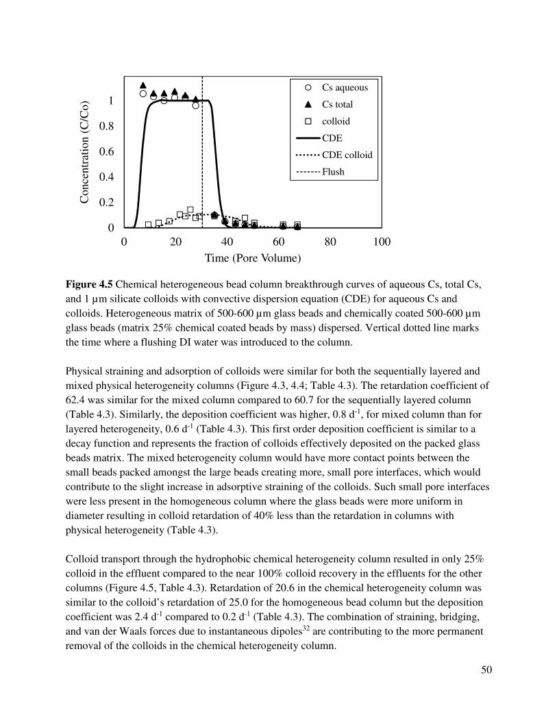
50
Figure 4.5 Chemical heterogeneous bead column breakthrough curves of aqueous Cs, total Cs,
and 1 µm silicate colloids with convective dispersion equation (CDE) for aqueous Cs and
colloids. Heterogeneous matrix of 500-600 µm glass beads and chemically coated 500-600 µm
glass beads (matrix 25% chemical coated beads by mass) dispersed. Vertical dotted line marks
the time where a flushing DI water was introduced to the column.
Physical straining and adsorption of colloids were similar for both the sequentially layered and
mixed physical heterogeneity columns (Figure 4.3, 4.4; Table 4.3). The retardation coefficient of
62.4 was similar for the mixed column compared to 60.7 for the sequentially layered column
(Table 4.3). Similarly, the deposition coefficient was higher, 0.8 d-1, for mixed column than for
layered heterogeneity, 0.6 d-1 (Table 4.3). This first order deposition coefficient is similar to a
decay function and represents the fraction of colloids effectively deposited on the packed glass
beads matrix. The mixed heterogeneity column would have more contact points between the
small beads packed amongst the large beads creating more, small pore interfaces, which would
contribute to the slight increase in adsorptive straining of the colloids. Such small pore interfaces
were less present in the homogeneous column where the glass beads were more uniform in
diameter resulting in colloid retardation of 40% less than the retardation in columns with
physical heterogeneity (Table 4.3).
Colloid transport through the hydrophobic chemical heterogeneity column resulted in only 25%
colloid in the effluent compared to the near 100% colloid recovery in the effluents for the other
columns (Figure 4.5, Table 4.3). Retardation of 20.6 in the chemical heterogeneity column was
similar to the colloid’s retardation of 25.0 for the homogeneous bead column but the deposition
coefficient was 2.4 d-1 compared to 0.2 d-1 (Table 4.3). The combination of straining, bridging,
and van der Waals forces due to instantaneous dipoles32 are contributing to the more permanent
removal of the colloids in the chemical heterogeneity column.
0
0.2
0.4
0.6
0.8
1
0 20 40 60 80 100
Conce
ntr
atio
n (
C/C
o)
Time (Pore Volume)
Cs aqueous
Cs total
colloid
CDE
CDE colloid
Flush

51
Cesium transport
Aqueous Cs transport through the columns was modeled using Cs portioning coefficient data
(Table 4.2), velocity from column discharge (Table 4.2), and dispersion data based on I transport
(Figure 4.6) through columns (Table 4.2 – 4.3; Figure 4.2 – 4.5). The fit of the aqueous Cs
breakthrough data to the CDE model ranged from r2=0.86 for the mixed physical heterogeneity
to r2 =0.94 for chemical heterogeneity column (Table 4.3). These fits are reasonable for the
aqueous Cs data generated, where the noise in the data can be attributed to the small pore size of
the column and resultant samples which were subsampled. Total Cs was less than 5% greater
than aqueous Cs values, which is within the experimental quality limits. So it is not definitive
that Cs transport was being facilitated by colloids beyond the Cs already adsorbed in the CsI +
colloid suspension, which at its maximum is 7% of the total Cs based on maximum adsorbed Cs
from partitioning coefficients. It can be seen that after the colloid suspension is flushed out with
deionized water containing no colloids (Figure 4.2-4.5) that the colloids no longer are associated
with Cs in the effluent. The homogeneous column total surface area of the packed beads was
0.07 m2 whereas the colloid total surface area was 0.008 m2, for total colloids introduced, so in
this case there was an order of magnitude more surface area for the packed glass bead matrix
compared to the colloid’s total surface area. With increased interaction with bead surfaces due to
adsorption, straining, and bridging of colloids, it is reasonable that Cs would be stripped from the
colloids. In experimental conditions where natural sediment known to strongly sorb Cs forms the
matrix, 30-40% colloid facilitated transport of Cs has been documented in the effluent of a
column with pore velocities of 1400-14000 cm d-1.11 This is more pronounced with the delayed
breakthrough of colloids such as with the physical heterogeneity columns where effluent Cs was
below detection limits when the bulk of the colloids were flushed from the columns (Figure 4.3,
Figure 4.4). At this slow pore velocity and with the surface adsorption normalized to surface area
(Kd/SA) for colloids (421 mL m-2) being of similar magnitude with large uncoated glass beads
(106 mL m-2), Cs is striped from colloids and remains on the glass beads. The SA normalized
partitioning coefficient for the chemically coated beads (1026 mL m-2) is an order of magnitude
greater than the uncoated beads and the colloids, so this striping would occur in addition to the
retention of the colloids in the glass bead matrix making colloid facilitated transport of metals
like Cs unlikely to occur.

52
Figure 4.6 Initial I breakthrough for homogeneous matrix column, sequentially layered physical
heterogeneity matrix column, mixed physical heterogeneity matrix column, and chemical
heterogeneity matrix column. Full initial and receding I curves were used to develop
hydrodynamic dispersivity coefficients for each column found in Table 3.
4.4 CONCLUSION
When the colloids and porous matrix have similar surface properties at slow pore velocity
conditions, contaminants such as Cs will exhibit no facilitated transport by colloids. This is due
to the striping of Cs from the colloids onto the stationary matrix. The transport of colloids
through heterogeneously packed columns will also be retarded more than through homogenous
matrices. Sequentially layered physical heterogeneity will retard colloid transport through the
stationary porous media similar to mixed physical heterogeneities, and the Cs originally
adsorbed to the colloids will be stripped. When a hydrophobic chemical heterogeneity is present
in the stationary matrix, silica-based colloids will be significantly removed due to fast deposition
of colloids and not hydraulically transported through the matrix even with long flushing times
unless high flow rate is maintained.
This work has been published in Journal of Contaminant Hydrology in 2018. “Effect of chemical
and physical heterogeneities on colloid-facilitated cesium transport”, K Rod, W Um, J Chun, N
Wu, X Yin, G Wang, K Neeves. https://doi.org/10.1016/j.jconhyd.2018.03.012
0.00
0.20
0.40
0.60
0.80
1.00
0 1 2 3 4
Conce
ntr
atio
n (
C/C
o)
Time (Pore Volume)
Homogeneous
Layered Physical
Mixed Physical
Chemical

53
REFERENCES
1. de Jonge, L. W.; Kjaergaard, C.; Moldrup, P., Colloids and colloid-facilitated transport of
contaminants in soils: An introduction. Vadose Zone J. 2004, 3, (2), 321-325.
2. Jacobsen, O. H.; Moldrup, P.; Larsen, C.; Konnerup, L.; Petersen, L. W., Particle
transport in macropores of undisturbed soil columns. J. Hydrol. 1997, 196, (1-4), 185-203.
3. Karathanasis, A. D., Subsurface migration of copper and zinc mediated by soil colloids.
Soil Sci. Soc. Am. J. 1999, 63, (4), 830-838.
4. Kretzschmar, R.; Robarge, W. P.; Amoozegar, A., Influence of natural organic-matter on
colloid transport through saprolite. Water Resour. Res. 1995, 31, (3), 435-445.
5. Flury, M.; Czigany, S.; Chen, G.; Harsh, J. B., Cesium migration in saturated silica sand
and Hanford sediments as impacted by ionic strength. J. Contam. Hydrol. 2004, 71, (1-4), 111-
126.
6. McKinley, J. P.; Zeissler, C. J.; Zachara, J. M.; Serne, R. J.; Lindstrom, R. M.; Schaef, H.
T.; Orr, R. D., Distribution and retention of Cs-137 in sediments at the Hanford Site,
Washington. Environ. Sci. Technol. 2001, 35, (17), 3433-3441.
7. Mohanty, S. K.; Saiers, J. E.; Ryan, J. N., Colloid-Facilitated Mobilization of Metals by
Freeze-Thaw Cycles. Environ. Sci. Technol. 2014, 48, (2), 977-984.
8. Saiers, J. E.; Hornberger, G. M., Migration of Cs-137 through quartz sand: Experimental
results and modeling approaches. J. Contam. Hydrol. 1996, 22, (3-4), 255-270.
9. Xu, S. P.; Liao, Q.; Saiers, J. E., Straining of nonspherical colloids in saturated porous
media. Environ. Sci. Technol. 2008, 42, (3), 771-778.
10. Turner, N. B.; Ryan, J. N.; Saiers, J. E., Effect of desorption kinetics on colloid-
facilitated transport of contaminants: Cesium, strontium, and illite colloids. Water Resour. Res.
2006, 42, (12), 17.
11. Chen, G.; Flury, M.; Harsh, J. B.; Lichtner, P. C., Colloid-facilitated transport of cesium
in variably saturated Hanford sediments. Environ. Sci. Technol. 2005, 39, (10), 3435-3442.
12. Flury, M.; Mathison, J. B.; Harsh, J. B., In situ mobilization of colloids and transport of
cesium in Hanford sediments. Environ. Sci. Technol. 2002, 36, (24), 5335-5341.
13. McNew, C. P.; Kananizadeh, N.; Li, Y. S.; LeBoeuf, E. J., The attachment of colloidal
particles to environmentally relevant surfaces and the effect of particle shape. Chemosphere
2017, 168, 65-79.
14. Shani, C.; Weisbrod, N.; Yakirevich, A., Colloid transport through saturated sand
columns: Influence of physical and chemical surface properties on deposition. Colloids and
Surfaces a-Physicochemical and Engineering Aspects 2008, 316, (1-3), 142-150.
15. Bradford, S. A.; Simunek, J.; Bettahar, M.; Tadassa, Y. F.; van Genuchten, M. T.; Yates,
S. R., Straining of colloids at textural interfaces. Water Resour. Res. 2005, 41, (10), 18.
16. Crist, J. T.; Zevi, Y.; McCarthy, J. F.; Throop, J. A.; Steenhuis, T. S., Transport and
retention mechanisms of colloids in partially saturated porous media. Vadose Zone J. 2005, 4,
(1), 184-195.

54
17. Zhang, Q. L.; Hassanizadeh, S. M.; Liu, B.; Schijven, J. F.; Karadimitriou, N. K., Effect
of hydrophobicity on colloid transport during two-phase flow in a micromodel. Water Resour.
Res. 2014, 50, (10), 7677-7691.
18. Baumann, T.; Werth, C. J., Visualization and modeling of polystyrol colloid transport in
a silicon micromodel. Vadose Zone J. 2004, 3, (2), 434-443.
19. Baumann, T.; Werth, C. J., Visualization of colloid transport through heterogeneous
porous media using magnetic resonance imaging. Colloids and Surfaces a-Physicochemical and
Engineering Aspects 2005, 265, (1-3), 2-10.
20. Guo, Y.; Huang, J. W.; Xiao, F.; Yin, X. L.; Chun, J.; Um, W.; Neeves, K. B.; Wu, N.,
Bead-Based Microfluidic Sediment Analogues: Fabrication and Colloid Transport. Langmuir
2016, 32, (36), 9342-9350.
21. Liu, Z. R.; Flury, M.; Harsh, J. B.; Mathison, J. B.; Vogs, C., Colloid mobilization in an
undisturbed sediment core under semiarid recharge rates. Water Resour. Res. 2013, 49, (8),
4985-4996.
22. Blake, G. R.; Hartge, K. H., Particle Density. In Methods of Soil Analysis, Part 1,
Physical and Mineralogical Methods, 2nd Edition, Klute, A., Ed. Soil Science Society of
America: Madison, Wisconsin, 1986; pp 377-382.
23. Brunauer, S.; Emmett, P. H.; Teller, E., Adsorption of gases in multimolecular layers. J.
Am. Chem. Soc. 1938, 60, 309-319.
24. ASTM Standard Test Method for Distribution Coefficients of Inorganic Species by the
Batch Method; C1733-10; ASTM International: West Conshohken, PA, 2010; pp 1-8.
25. Kaiser, K.; Guggenberger, G., The role of DOM sorption to mineral surfaces in the
preservation of organic matter in soils. Organic Geochemistry 2000, 31, (7-8), 711-725.
26. Chrysikopoulos, C. V.; Syngouna, V. I., Effect of Gravity on Colloid Transport through
Water-Saturated Columns Packed with Glass Beads: Modeling and Experiments. Environ. Sci.
Technol. 2014, 48, (12), 6805-6813.
27. Toride, N.; Leij, F. J.; van Genuchten, M. T. The CXTFIT code for estimating transport
parameters from laboratory or field tracer experiments. Version 2.1; Report #137; U.S. Salinity
Laboratory, U.S. Department of Agriculture: Riverside, CA, 1999; p 117.
28. Pierce, E. M.; Reed, L. R.; Shaw, W. J.; McGrail, B. P.; Icenhower, J. P.; Windisch, C.
F.; Cordova, E. A.; Broady, J., Experimental determination of the effect of the ratio of B/Al on
glass dissolution along the nepheline (NaAlSiO4)-malinkoite (NaBSiO4) join. Geochim.
Cosmochim. Acta 2010, 74, (9), 2634-2654.
29. Dumat, C.; Quiquampoix, H.; Staunton, S., Adsorption of cesium by synthetic clay-
organic matter complexes: Effect of the nature of organic polymers. Environ. Sci. Technol. 2000,
34, (14), 2985-2989.
30. Fan, Q. H.; Yamaguchi, N.; Tanaka, M.; Tsukada, H.; Takahashi, Y., Relationship
between the adsorption species of cesium and radiocesium interception potential in soils and
minerals: an EXAFS study. J. Environ. Radioact. 2014, 138, 92-100.

55
31. Sen, T. K.; Khilar, K. C., Review on subsurface colloids and colloid-associated
contaminant transport in saturated porous media. Adv. Colloid Interface Sci. 2006, 119, (2-3),
71-96.
32. Horvolgyi, Z.; Medveczky, G.; Zrinyi, M., On the structure formation of hydrophobed
particles in the boundary-layer of water and octane phases. Colloid Polym. Sci. 1993, 271, (4),
396-403.
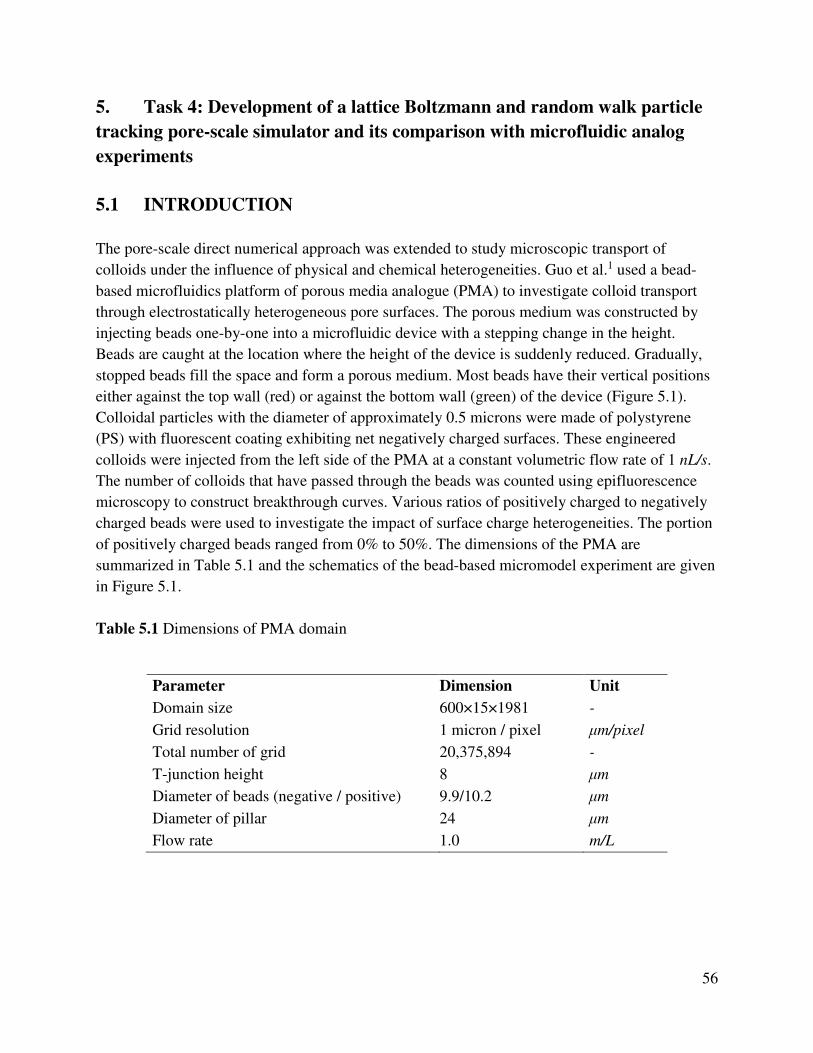
56
5. Task 4: Development of a lattice Boltzmann and random walk particle
tracking pore-scale simulator and its comparison with microfluidic analog
experiments
5.1 INTRODUCTION
The pore-scale direct numerical approach was extended to study microscopic transport of
colloids under the influence of physical and chemical heterogeneities. Guo et al.1 used a bead-
based microfluidics platform of porous media analogue (PMA) to investigate colloid transport
through electrostatically heterogeneous pore surfaces. The porous medium was constructed by
injecting beads one-by-one into a microfluidic device with a stepping change in the height.
Beads are caught at the location where the height of the device is suddenly reduced. Gradually,
stopped beads fill the space and form a porous medium. Most beads have their vertical positions
either against the top wall (red) or against the bottom wall (green) of the device (Figure 5.1).
Colloidal particles with the diameter of approximately 0.5 microns were made of polystyrene
(PS) with fluorescent coating exhibiting net negatively charged surfaces. These engineered
colloids were injected from the left side of the PMA at a constant volumetric flow rate of 1 nL/s.
The number of colloids that have passed through the beads was counted using epifluorescence
microscopy to construct breakthrough curves. Various ratios of positively charged to negatively
charged beads were used to investigate the impact of surface charge heterogeneities. The portion
of positively charged beads ranged from 0% to 50%. The dimensions of the PMA are
summarized in Table 5.1 and the schematics of the bead-based micromodel experiment are given
in Figure 5.1.
Table 5.1 Dimensions of PMA domain
Parameter Dimension Unit
Domain size 600×15×1981 -
Grid resolution 1 micron / pixel μm/pixel
Total number of grid 20,375,894 -
T-junction height 8 μm
Diameter of beads (negative / positive) 9.9/10.2 μm
Diameter of pillar 24 μm
Flow rate 1.0 m/L
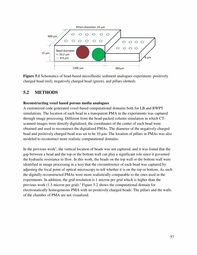
57
Figure 5.1 Schematics of bead-based microfluidic sediment analogues experiment: positively
charged bead (red), negatively charged bead (green), and pillars (dotted).
5.2 METHODS
Reconstructing voxel based porous media analogues
A customized code generated voxel-based computational domains both for LB and RWPT
simulations. The location of each bead in a transparent PMA in the experiments was captured
through image processing. Different from the bead-packed column simulation in which CT-
scanned images were directly digitalized, the coordinates of the center of each bead were
obtained and used to reconstruct the digitalized PMAs. The diameter of the negatively charged
bead and positively charged bead was set to be 10 µm. The location of pillars in PMAs was also
modeled to reconstruct more realistic computational domains.
In the previous work1, the vertical location of beads was not captured, and it was found that the
gap between a bead and the top or the bottom wall can play a significant role since it governed
the hydraulic resistance to flow. In this work, the beads on the top wall or the bottom wall were
identified in image processing in a way that the circumference of each bead was captured by
adjusting the focal point of optical microscopy to tell whether it is on the top or bottom. As such
the digitally reconstructed PMAs were more realistically comparable to the ones used in the
experiments. In addition, the grid resolution is 1 micron per grid which is higher than the
previous work (1.5 micron per grid).1 Figure 5.2 shows the computational domain for
electrostatically homogeneous PMA with no positively charged beads. The pillars and the walls
of the chamber of PMA are not visualized.
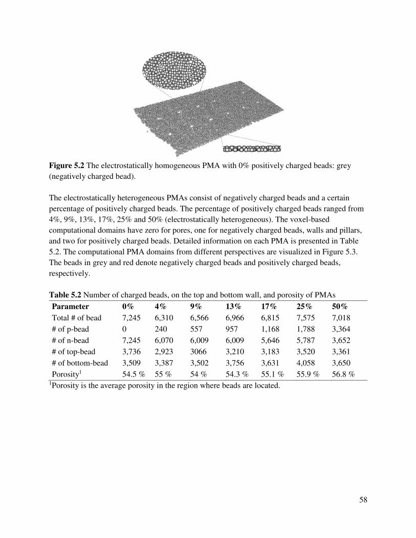
58
Figure 5.2 The electrostatically homogeneous PMA with 0% positively charged beads: grey
(negatively charged bead).
The electrostatically heterogeneous PMAs consist of negatively charged beads and a certain
percentage of positively charged beads. The percentage of positively charged beads ranged from
4%, 9%, 13%, 17%, 25% and 50% (electrostatically heterogeneous). The voxel-based
computational domains have zero for pores, one for negatively charged beads, walls and pillars,
and two for positively charged beads. Detailed information on each PMA is presented in Table
5.2. The computational PMA domains from different perspectives are visualized in Figure 5.3.
The beads in grey and red denote negatively charged beads and positively charged beads,
respectively.
Table 5.2 Number of charged beads, on the top and bottom wall, and porosity of PMAs
Parameter 0% 4% 9% 13% 17% 25% 50%
Total # of bead 7,245 6,310 6,566 6,966 6,815 7,575 7,018
# of p-bead 0 240 557 957 1,168 1,788 3,364
# of n-bead 7,245 6,070 6,009 6,009 5,646 5,787 3,652
# of top-bead 3,736 2,923 3066 3,210 3,183 3,520 3,361
# of bottom-bead 3,509 3,387 3,502 3,756 3,631 4,058 3,650
Porosity1 54.5 % 55 % 54 % 54.3 % 55.1 % 55.9 % 56.8 % 1Porosity is the average porosity in the region where beads are located.
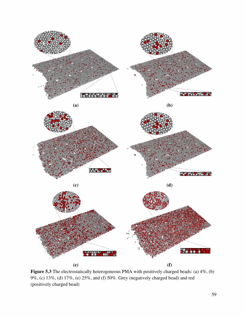
59
(a) (b)
(c) (d)
(e) (f)
Figure 5.3 The electrostatically heterogeneous PMA with positively charged beads: (a) 4%, (b)
9%, (c) 13%, (d) 17%, (e) 25%, and (f) 50%. Grey (negatively charged bead) and red
(positively charged bead)
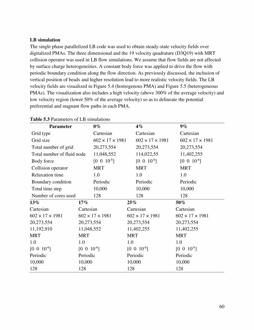
60
LB simulation
The single phase parallelized LB code was used to obtain steady-state velocity fields over
digitalized PMAs. The three dimensional and the 19 velocity quadrature (D3Q19) with MRT
collision operator was used in LB flow simulations. We assume that flow fields are not affected
by surface charge heterogeneities. A constant body force was applied to drive the flow with
periodic boundary condition along the flow direction. As previously discussed, the inclusion of
vertical position of beads and higher resolution lead to more realistic velocity fields. The LB
velocity fields are visualized in Figure 5.4 (homogenous PMA) and Figure 5.5 (heterogeneous
PMAs). The visualization also includes a high velocity (above 300% of the average velocity) and
low velocity region (lower 50% of the average velocity) so as to delineate the potential
preferential and stagnant flow paths in each PMA.
Table 5.3 Parameters of LB simulations
Parameter 0% 4% 9%
Grid type Cartesian Cartesian Cartesian
Grid size 602 × 17 × 1981 602 × 17 × 1981 602 × 17 × 1981
Total number of grid 20,273,554 20,273,554 20,273,554
Total number of fluid node 11,048,552 114,022,55 11,402,255
Body force [0 0 10-6] [0 0 10-6] [0 0 10-6]
Collision operator MRT MRT MRT
Relaxation time 1.0 1.0 1.0
Boundary condition Periodic Periodic Periodic
Total time step 10,000 10,000 10,000
Number of cores used 128 128 128
13% 17% 25% 50%
Cartesian Cartesian Cartesian Cartesian
602 × 17 × 1981 602 × 17 × 1981 602 × 17 × 1981 602 × 17 × 1981
20,273,554 20,273,554 20,273,554 20,273,554
11,192,910 11,048,552 11,402,255 11,402,255
MRT MRT MRT MRT
1.0 1.0 1.0 1.0
[0 0 10-6] [0 0 10-6] [0 0 10-6] [0 0 10-6]
Periodic Periodic Periodic Periodic
10,000 10,000 10,000 10,000
128 128 128 128

61
(a)
(b) (c)
Figure 5.4 The LB velocity field of 0% electrostatically homogeneous PMA: (a) the velocity
over the entire PMA, (b) the 3D velocity fields above 300% of (orange) below 50% (blue) of
the average velocity with beads (grey), and (c) in 2D.
(a) 4% (b) 9%

62
(c) 13% (d) 17%
(e) 25% (f) 50%
Figure 5.5 The LB velocity fields of electrostatically heterogeneous PMA: plane view at 4 μm
above the bottom, and the velocity above 300% and below 50%of the average velocity.
RWPT simulation for electrostatically homogeneous PMA
The random walk particle tracking (RWPT) code was used to solve advective and diffusive
movement of colloids through the PMAs. In RWPT, the steady-state velocity fields obtained
from LB simulations were used to determine the advective displacement of colloids. The
diffusive displacement by random motion is added to locate the final position of colloidal
particles. The random motion in RWPT is modeled isotropic in every direction. No flux
boundary condition was implemented in RWPT using a specular reflection method by which a
tracer does a “mirror-like” reflection when it hits the solid surface during the course of advective
or diffusive movement. The colloids were modeled as non-aggregative volumeless point tracers
with no tracer-to-tracer interactions considered.
The electrostatically homogeneous experiment, free of charge interactions, was first taken to be
investigated. The self-diffusion coefficient of a nanoparticle used in the experiment was given as

63
Dm = 8.58×10⁻¹³ m2/s. The dimensionless self-diffusion coefficient of RWPT was chosen to
match the experimental Péclet number. To set the boundary conditions of RWPT, the injection
condition of the experiment was examined and it was found that the injection concentration of
the experiment was not perfectly held constant (Figure 5.6). The injection concentration rapidly
built up and leveled off at approximately 8 to 10 pore volume (PV). At 38 about 38 PV, the
injection stream at the inlet was stopped and the concentration starts decreasing from 38 to 48
PV, i.e., the elusion phase. To account for this experimental detail, RWPT was coded to track
the actual inlet concentration of the experiments.
(a) (b)
Figure 5.6 Actual inlet injection concentration (a) and the injection concentration normalized
by the average steady state concentration (b).
The logistics growth curves were used to obtain a mathematical expression corresponding to the
actual inlet concentration profile. The constants (a1, b1, c1, and d1) in the logistics growth curve
(Eq. 5.1) were obtained by fitting the actual inlet concentration profile (Figure 5.7). In RWPT, a
random probability is assigned to every tracer in the inlet region (0 to 100 in z direction) and
compared with the probability P in Eq. 5.1 at a given pore volume (tR). If the random probability
is greater than P, such tracers are nullified not to be counted in the construction of breakthrough
curves. Figure 5.7 shows the mathematical model (a) and the simulated injection profile (b)
relative to the normalized injection concentration of the experiment. The simulated injection
concentration was in good agreement with that of the experiments with a tolerable degree of
statistical noise.
1
11
1
( )1 R
R b t
cP t d
a e−
= −+
(5.1)

64
(a) (b)
Figure 5.7 Actual inlet injection concentration
With the controlled inlet concentration profile, RWPT successfully generated the breakthrough
curve that is in good agreement with that of the electrostatically homogeneous experiment
(Figure 5.8). The simulated breakthrough curve with no inlet control is also presented for
comparison (Figure 5.8b). As previously discussed, this breakthrough level comparison confirms
that our pore-scale simulations have successfully simulated advection-dispersion by solving
microscopic advection-diffusion of colloid in porous media under the given Péclet number flow
regime. This breakthrough level comparison additionally confirms that the excess retardation in
the breakthrough curves stemmed dominantly from the relaxed inlet concentration of the
experiment.
(a) (b)
Figure 5.8 Comparison of the BTCs between the experiment and simulation with controlled
inlet concentration (a) and with a constant inlet concentration (b) for comparison: experiment
(green) and simulation (blue).

65
RWPT simulation for electrostatically heterogeneous PMA
The propagation of colloids through chemically heterogeneous microfluidic sediment analogues
was then investigated. The heterogeneous PMAs contained a certain percentage of positively
charged beads to investigate the effects of surface charge heterogeneities onto the retention
kinetics of colloids under attractive interaction by electrostatic force. The retention process of
colloids is typically irreversible while that of solutes is reversible.2 Colloids retained due to
surface charge heterogeneities remain on the surfaces with no chances of release. Thus, colloid
retention is a kinetic process rather than an equilibrium process.2 It was also observed in our
microfluidics experiments that retention occurred in an irreversible manner such that colloids
once retained on the surface of positively charged beads were not remobilized to the solution
since the attractive forces are much greater than fluid drag forces.3
Irreversible retention processes due to surface charge heterogeneities were modeled in RWPT by
the inclusion of the concept of “interaction length”. The interaction length defines a region of
effective attractive interaction around a positively charged bead and it was assumed that colloids
that entered this region were retained permanently. If a “free” tracer falls within the prescribed
interaction range of a positively charged bead, it turns to a “retained” tracer with its location of
retention recorded. The tracer captured within the interaction length keeps moving to the outlet
to satisfy the periodic boundary condition but they are not counted for the construction of
breakthrough curves. A “null” tracer turns to a “free” tracer when it exits the current domain and
this procedure repeats until the end of simulation (Figure 5.9). We assumed that the repulsive
interaction between negatively charged beads and colloids was negligible based on the
observations in the experiments. Therefore, it is simulating the kinetic removal of colloids under
favorable conditions.
Figure 5.9 Illustration of a tracer falling into the “interception length” (grey) of a positively
charged bead (p-bead), turning from a “free tracer (white)” to a “null tracer (grey)” after being
retained (yellow).

66
Exact mechanism of this retention kinetics is also an area of active research since various scales
of interactions are inter-winded. In mechanistic approaches, forces due to fluid drag, diffusion,
gravity, and DLVO forces (van der Waals and electric double layer) are considered.4,5 As
observed in the microfluidics experiments, the electrostatic attraction between net-negatively
charged colloids and positively charged beads was the most dominant mechanism of the
retention process. Then the electrostatic “interaction range” can be theoretically calculated by
evaluating the free energy between a colloidal particle and the surface of a bead. It was assumed
that a colloidal particle is retained on the surface of a bead if the free energy is ten times greater
than the thermal energy. The electrostatic interaction range of 500 nm was used in RWPT.
The dynamics pertaining to colloid retention inevitably involves variable kinetics as a colloidal
particle approaches the surfaces of porous media.6 At the early stage when most of the surface of
solid matrix is not occupied, the rate of retention is almost constant exhibiting its maximum
retention capacity. As more colloids cover the surface of the solid phase, the retention rate
decreases or increase as the layer of colloids accumulated on the surface slows down or speed up
the rate of deposition depending on the interaction between retained colloids and free colloids
approaching the surface. This is so called the “surface coverage effect” or “blocking effect”.7
The surface coverage effect is usually modeled by either a linear or non-linear dynamics
blocking function. A linear Langmurian dynamic blocking function assumes a linear dependence
on surface coverage while a non-linear dynamic blocking function uses a power law relation. In
either linear or non-linear model, the rate of deposition is a function of solid phase surfaces that
are not blocked by colloids.
The surface coverage effect was also observed in our experiments. In order to account for this,
the capacity of retention of a single positively charged bead was estimated by performing a
separate experiment. The number of colloids collected by a positively charged bead under the
same flow regime as the experiments for much extended time was counted at 82 (Nbead) on
average. The ratio of the number of tracers in RWPT to the number of colloidal particle is
approximately 150 (the colloid to tracer ratio), which means 150 tracers in RWPT are
statistically equivalent to one colloidal particle in the experiment. Therefore, the capacity of a
single node on the surface of a positively charged bead can be estimated by scaling the average
number of colloids observed in the experiment by the surface area of a bead. Then, the capacity
of electrostatic retention of a single node on the surface of a positively charged bead (nnode) is
estimated (Eq. 5.2). In RWPT, a probability of retention of a single node on the surface of a
positively charged bead decreases linearly from the prescribed maximum number to zero
depending on the number of tracers retained.
colloid-to-tracer ratio40
surface area of beadnode beadn N= × ≃ (5.2)
The linear Langmuir adsorption model follows
( ) 1B θ βθ= − (5.3)
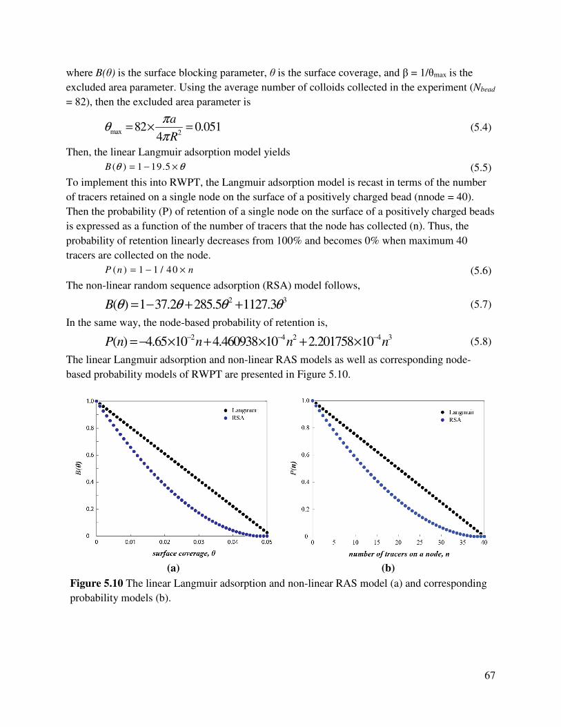
67
where B(θ) is the surface blocking parameter, θ is the surface coverage, and β = 1/θmax is the
excluded area parameter. Using the average number of colloids collected in the experiment (Nbead
= 82), then the excluded area parameter is
max 282 0.051
4
a
R
πθ
π= × = (5.4)
Then, the linear Langmuir adsorption model yields
( ) 1 19.5B θ θ= − × (5.5)
To implement this into RWPT, the Langmuir adsorption model is recast in terms of the number
of tracers retained on a single node on the surface of a positively charged bead (nnode = 40).
Then the probability (P) of retention of a single node on the surface of a positively charged beads
is expressed as a function of the number of tracers that the node has collected (n). Thus, the
probability of retention linearly decreases from 100% and becomes 0% when maximum 40
tracers are collected on the node.
( ) 1 1 / 40P n n= − × (5.6)
The non-linear random sequence adsorption (RSA) model follows,
2 3( ) 1 37.2 285.5 1127.3B θ θ θ θ= − + + (5.7)
In the same way, the node-based probability of retention is,
2 4 2 4 3( ) 4.65 10 4.460938 10 2.201758 10P n n n n− − −= − × + × + × (5.8)
The linear Langmuir adsorption and non-linear RAS models as well as corresponding node-
based probability models of RWPT are presented in Figure 5.10.
(a) (b)
Figure 5.10 The linear Langmuir adsorption and non-linear RAS model (a) and corresponding
probability models (b).

68
5.3 RESULTS AND DISCUSSION
Breakthrough curves of electrostatically heterogeneous PMAs
With the controlled inlet concentration, the interaction length and the surface coverage effect,
RWPT simulations were performed for all the heterogeneous PMAs. The RWPT simulation
parameters are summarized in Table 5.4 and the simulated breakthrough curves relative to those
of the experiments are all presented in Figure 5.11.
Table 5.4 Parameters of RWPT simulations
Parameter 0% 4% 9%
Grid type Cartesian Cartesian Cartesian
Grid size 602 × 17 × 1981 602 × 17 × 1981 602 × 17 × 1981
Total number of grid 20,273,554 20,273,554 20,273,554
Total number of fluid node 11,048,552 114,022,55 11,402,255
Total number of tracer 54,997 57,749 56,963
Average velocity 4.46456×10⁻⁶ 5.19594×10⁻⁶ 4.71715×10⁻⁶
Maximum velocity 1.40242×10⁻⁴ 6.53804×10⁻⁵ 5.68874×10⁻⁵
Diffusion coefficient 3.92023×10⁻⁸ 4.56244×10⁻⁸ 4.142026×10⁻⁸
Time step size 3.36466×10³ 6.67901×10³ 8.005230×10³
Total time step
140×24782
140 ×11773
140×11261
13% 17% 25% 50%
Cartesian Cartesian Cartesian Cartesian
602 × 17 × 1981 602 × 17 × 1981 602 × 17 × 1981 602 × 17 × 1981
20,273,554 20,273,554 20,273,554 20,273,554
11,192,910 11,048,552 114,022,55 11,402,255
55717 56,346 54,493 55,871
4.834690E-06 4.93270×10⁻⁶ 4.65152×10⁻⁶ 5.28837×10⁻⁶
7.266740E-05 6.00841×10⁻⁵ 5.94276×10⁻⁵ 6.38512×10⁻⁵
4.245235E-08 4.33130×10⁻⁸ 4.08440×10⁻⁸ 4.64360×10⁻⁸
6.338310E+03 7.58285×10³ 7.68342×10³ 7.13255×10³
140×12543 140×10375 140 ×9263 140×9082
128 128 128 128
Figure 5.11 shows that the numerical solutions of our pore-scale simulations are very good
agreement with the experiments. Taking the 4% PMA for example, the normalized effluent
concentration builds up until 7 pore volume (PV), and then the rate of increase slows down,
showing two distinctive slops from 7 PV. The initial build-up region is the typical characteristic
of advection-dispersion in porous media. The kinetic retention removes or filters colloids

69
traveling near the positively charged. As such the effluent concentration stabilizes at about 40%
at 7 PV. Past 7 PV, the concentration increases at a slower rate because the surfaces of positively
charged beads are being covered by retained colloids. As the surfaces are being excluded further
by retained colloids, retention capacity decreases as modeled using the linear Langmurian
blocking and non-linear random sequence adsorption (RSA) model. Thus, the increase in
concentration at a slow rate past 7 PV is attributed to this surface coverage effect. At 38 PV, the
concentration drops as the injection steam is stopped.
Our pore-scale simulations combined with 1) the inlet concentration relaxation, 2) the interaction
range for kinetic retention, and 3) blocking functions for surface coverage effect, have
successfully predicted the early time build-up (0 to 7 PV), the increase at a slower rate due to
surface exclusion (7 PV to 38 PV), and the elusion phase (38 PV to 52 PV). These comparisons
on the level of breakthrough curves once again confirms that the dominant mechanisms that
controlled advection-dispersion and retention of colloids under the effect of surface charge
heterogeneity was the irreversible kinetic retention process due to electrostatic interactions
combined with surface coverage effects. Therefore, our modeling approaches to incorporating
the kinetic retention and surface exclusion are successfully validated. When it comes to the linear
and non-linear finite adsorptive models, there is only a subtle difference between the linear
Langmurian blocking function and the non-linear RSA model. This indicates that surface
exclusion behavior did not have a significant impact under the given flow and transport regime
in the experiments.
For the PMAs with higher percentage of positively charged bead (17, 25, and 50%), the effluent
concentration profiles predicted by our pore-scale simulations were slightly higher than those of
the experiments. There may be several reasons: 1) it was observed in the experiments that some
colloids were trapped near negatively charged beads. This is probably because of finite size of
colloid particles as some of pore spaces were not large enough due to geometric configuration so
that a few colloidal particles could have been trapped. Since a colloidal particle was modeled as
a volumeless point particle in our RWPT, the retention due to finite size cannot be capture. 2)
The accuracy of image processing tends to become less accurate at the edges of the PMA box. If
the pore spaces on both sides of the PMA box were overestimated, preferential flow paths were
made in LB velocity filed. Then more tracers than what actually moved through these flow paths
result in the overestimation of the effluent concentration.

70
(a) (b)
(c) (d)
(e) (f)
Figure 5.11 The breakthrough curves of electrostatically heterogeneous PMAs with 4% (a),
9% (b), 13% (c), 17% (d) 25% (e), and 50% (f) of positively charged bead: the interception
length = 500 nm and the nodal retention capacity n = 40.

71
5.4 CONCLUSION
Our pore-scale numerical simulator was extended to colloid transport under the influence of
surface charge heterogeneities. We first reproduced the breakthrough curve of electrostatically
homogeneous PMA. The inlet concentration in our simulation was relaxed by matching the
experimental one, and we obtained a breakthrough curve that agreed well with the experimental
breakthrough curve. This case of electrostatically homogeneous PMA confirmed that our pore-
scale modeling approach using LB and RWPT is applicable to colloid transport in the high Péclet
number flow regime. We then incorporated colloid-surface interaction range and dynamic
blocking functions to simulate irreversible colloid deposition in electrostatically heterogeneous
PMAs and obtained breakthrough curves that are good agreement with those of PMAs.

72
REFERENCE
(1) Guo, Y., Huang, J., Xiao, F., Yin, X., Chun, J., Um, W., … Wu, N. (2016). Bead-Based
Microfluidic Sediment Analogues: Fabrication and Colloid Transport. Langmuir, 32(36),
9342–9350. https://doi.org/10.1021/acs.langmuir.6b02184
(2) Johnson, P. R., Sun, N., & Elimelech, M. (1996). Colloid Transport in Geochemically
Heterogeneous Porous Media : Modeling and Measurements Colloid Transport in
Geochemically Heterogeneous Porous Media : Modeling and Measurements. Environmental
Science & Technology, 30(11), 3284–3293. https://doi.org/10.1021/es960053
(3) Bergendahl, J., & Grasso, D. (1999). Prediction of colloid detachement in a model porous
media: Thermodynamics. American Institute of Chemical Engineers Journal, 45(3), 475–
484. https://doi.org/10.1016/S0009-2509(99)00422-4
(4) Derjaguin, B., & Landau, L. (1993). Theory of the stability of strongly charged lyophobic
sols and of the adhesion of strongly charged particles in solutions of electrolytes. Progress
in Surface Science, 43(1–4), 30–59. https://doi.org/10.1016/0079-6816(93)90013-L
(5) Verwey, E. J. ., & Overbeek, J. T. G. (1948). Theory of the Stability of Lyophobic Colloids.
Amsterdam, Netherlands: Elsevier.
(6) Molins, S., Trebotich, D., Steefel, C. I., & Shen, C. (2012). An investigation of the effect of
pore scale flow on average geochemical reaction rates using direct numerical simulation.
Water Resources Research, 48(3), 1–11. https://doi.org/10.1029/2011WR011404
(7) Johnson, P. R., & Elimelech, M. (1995). Dynamics of Colloid Deposition in Porous Media:
Blocking Based on Random Sequential Adsorption. Langmuir, 11(3), 801–812.
https://doi.org/10.1021/la00003a023

73
6. Task 5: Development of a lattice Boltzmann pore-scale and random
walk particle tracking simulator and its comparison with column experiments
6.1 INTRODUCTION
Advection-dispersion of reactive and non-reactive species in porous media is a subject of active
research in many branches of science and engineering including biology, hydrology,
environmental engineering and petroleum engineering. A number of transport models have been
developed and applied successfully for macro-scale or field scale problems. The mathematical
foundation for these classical transport models is to apply physical laws such as mass and
momentum conservation over a representative element volume (REV).1,2 Traditional approaches,
whether analytical or numerical, solve the governing equation in the form of partial differential
equations (PDEs) with given initial and boundary conditions. Analytical solutions for some
simple problems are still efficient tools to understand and analyze laboratory column
experiments, e.g., those for the one dimensional advection-dispersion equation (1D-ADE)3.
Analytic models are, however, limited in that they are solved on the assumptions of uniform flow
and simple boundary conditions. For more complex problems, numerical methods, mostly
borrowed from computational fluid dynamics (CFD), are preferred to solve discretized PDEs
with known coefficients and given boundary conditions4. All of the above approaches, however,
work over the scale of an REV and pore-scale features of porous medium are averaged out. As
such it is difficult to reveal and establish, using existing approaches, connections between pore-
scale physical and chemical heterogeneities and continuum-scale transport properties.
Such connections can be achieved using pore-scale simulations that explicitly consider complex
pore and solid geometries and solute-solvent-solid interactions5. Pore or sub-pore level processes
that affect macroscopic behavior are modeled on explicit representations of porous media. The
governing equations of flow and transport are solved with fundamental laws of mass and
momentum balance and boundary conditions satisfied at this level. In pore-scale direct numerical
simulations, the governing equations are solved on actual images of porous media. With complex
features of the pore structure honored, the resulting velocity fields naturally preserve variabilities
and non-uniformities due to tortuous paths of porous media.
The first step in the workflow of pore-scale direct numerical simulations is to create a three-
dimensional pore-scale model of a porous medium. Creating a realistic three dimensional (3D)
quantitative description of the pore geometry of a porous medium is an essential step in the
studies of flow and transport.5,6 X-ray microtomography (XMT) or micro-CT scanners are the
most widely used imaging tools in the studies of geologic material and the typical resolution is a
few microns.7-9 Noises and artifacts in the images obtained are filtered out before being
segmented into phase types, i.e., pores and grains. This process is known as image
segmentation10. Then the segmented images are recombined to reproduce a three-dimensional
voxel-based computational replica of porous media. The second step is solving flow and

74
transport using numerical methods, e.g., computational fluid dynamics (CFD) methods, 2) the
smoothed particle hydrodynamics (SPH) method, 3) and 3) the Lattice-Boltzmann method.
In this study, pore-scale simulation used lattice Boltzmann (LB) and a random walk particle
tracking method (RWPT) to solve advection-diffusion of a solute or a colloidal particle. Both LB
and RWPT codes have been parallelized to reduce the computational time. The RWPT code
generates tracer concentration profiles at the outlet (i.e., breakthrough curve or BTC). To
generate data that are comparable to the column experiments, image processing routines were
developed to digitalize images of the columns used in the experiments to build the simulation
domain needed by LB and RWPT simulations. The digitalized column contains about 49.5
million voxels (169 × 169 × 1732) and the number of fluid voxels is approximately 10 million.
CT-scanned images were processed using thresholds that recover the porosity of the real bead-
packed column. LB simulation was used to obtain the velocity field in the column. Using the
average advection velocity from the LB simulation, input parameters for the RWPT simulation
were determined to match the Péclet number of the column experiment. The breakthrough curves
of the column experiment for Iodide (I−) were obtained and compared with the experiment. This
approach has extended to simulate the equilibrium partition of aqueous Cesium by a probabilistic
approach to reproduce the retardation observed in experiments.
6.2 METHODS
Digitalization of a bead-packed column
A computer code to process CT-scanned images (2000 images, 298 KB and 525 × 582 pixels
each) of bead-packed columns used in the column experiments was developed. A binary
segmentation was implemented to differentiate glass beads and void spaces inside the column
and generated the computational domain for LB and RWPT simulations. The images were
visually inspected to determine the top and bottom sections of the column. Considering the
quality of images, the top was chosen at image # 0161 and the bottom was at image # 1881
(Figure 6.1). The original image files were then cropped to the size of 169 × 169 pixels to
remove much of the solid area outside the column. Otsu’s algorithm was applied to each cropped
image to find appropriate threshold values based on the histogram of the light intensity values.11
These images, as shown in Figure 6.1, show cross-sections of the column. A problem with the
images is that the inner surface of the column could not be clearly identified. To determine the
location of the inner surface of the column, an ellipse with adjustable major and minor axes and
orientation was used to fit the contour of the beads. After the inner surface was determined,
pixels inside the column were converted to binary (0: fluid; 1: solid) using different threshold
values till the porosity of images matches the porosity of the column in the experiment.
The real column used in the experiment was constructed by packing large 500-600 µm beads and
has a length of 10.26 cm and a diameter of 0.75 cm. The resolution of the images is 51.3 μm per
pixel and the distance between consecutive images is also 51.3 μm. A 500-600 µm bead was

75
resolved by 10 to 12 voxels. Figure 6.2 shows one example of the original CT-scanned image
and the binary image processed by the established threshold, where white denotes the pore space
(image # 1590). After thresholding, fluid and solid voxels are represented by zeros and ones,
respectively, in a Cartesian lattice system (Figure 6.2). The total 1,722 processed and stacked
images form the three dimensional digitalized column for flow and transport simulations (Figure
6.3).
Figure 6.1 The top and bottom images of the bead-packed column.
(a) (b)
(c) (d)
Figure 6.2 Procedure of image processing of CT-scanned column images to generate digitized
bead-packed column images (#1590): (a) original CT-scanned image, (b) cross-section of
column established by an ellipse, (c) cropped cross-section and (d) binary image of cropped
cross-section with pores (white) and grains (black).

76
Figure 6.3 Processed images of a bead-packed column are stacked to form a 3D digitalized
column for LB and RWPT simulations (only the surfaces of glass beads are visualized). The
size of the domain is 169×169×1722 in each direction. A three-quarter section view in the mid-
section of the column (from 700 to 1000) is also presented.
LB simulation
The LB code was used to obtain the velocity field within the digitalized bead-packed column.
The simulation was run to 20,000 LB time steps, at which point fluid flow in the column reached
the steady state. The computational domain size was 169 × 169 × 1732 including additional five
fluid layers on both ends of the column in the z direction to maintain periodicity of the
computational domain in the z direction. A constant body force was applied in the z-direction to
drive the fluid flow. The parameters of LB simulation are summarized in Table 6.1. The velocity
in the direction of fluid flow (z-direction) is visualized in Figure 6.4.
Table 6.1 Parameters of LB simulation of the column experiment
Parameter Value
Grid type Cartesian
Computational domain 169 × 169 × 1732
Total number of grid 49,467,652
Total number of fluid node 10,117,521
Body force [0 0 10-6]
Collision operator MRT
Relaxation time 1.0
Boundary condition Periodic
Simulation time step 20,000
# of CPUs 128

77
Figure 6.4 Visualization of z-velocity obtained from LB simulation: (a) z-velocity in the entire
column,
RWPT simulation of Iodide
In the column experiment, Iodide (I−) was used as a non-adsorbing solute since it does not adsorb
to glass beads. The velocity field obtained from LB simulation was passed to RWPT. The
diffusion coefficient and time step size of RWPT were chosen to match the experimental Péclet
number so that tracers in RWPT travel with the same advection-diffusion dynamics as the
experiment. In this study, the self-diffusion coefficients of Iodide (I−) and Cesium (+Cs) at
condition most comparable to the column experiment were taken from the work of Friedman and
Kennedy.12 Parameters of the RWPT simulation for Iodide transport (I-) are summarized in
Table 6.2.
Table 6.2 Parameters of RWPT simulation of Iodide transport.
Parameter Values
Grid type Cartesian
Size of computational domain 169 × 169 × 1732
Grid resolution 51.3 micron / pixel
Total number of grid 49,467,652
Total number of fluid node 10,117,521
Total number of tracer used 1,011,758
Superficial velocity from LBM 2.06616 × 10⁻⁷
Péclet number 14.04
Dimensionless diffusion coefficient 3.66 × 10⁻⁶
RWPT time step size 6.59064 × 10³
Duration of simulation 1.45211 × 10⁶ (5 PV)
Number of cores used 128

78
RWPT simulation of aqueous Cesium
Adsorption processes make some solutes move slower than the motion of bulk fluid. If
adsorption-desorption processes are reversible in equilibrium, they lead to equilibrium
retardation. This equilibrium retardation was also observed in the column experiment of cesium. 13 The RWPT code was modified to simulate solutes with adsorption-desorption equilibrium.
The equilibrium adsorption model was implemented by introducing a probability of adsorption
(Pa) and another probability of desorption (Pd) to determine whether a tracer adsorbs on or leaves
the surfaces of the solid phase. A random number (Prand) is generated when a tracer is intercepted
by an interface between the liquid and solid phases. If this random number is smaller than the
prescribed probability of adsorption (Pa > Prand), the tracer is adsorbed on the surface. If not (Pa
< Prand), a specular reflection is carried out to keep the tracer in solution. For tracers that are
already adsorbed, random numbers are generated to decide whether they should be sent back to
solution. An adsorbed tracer would leave solid surface if a random number, generated
specifically for this tracer, is smaller than the prescribed probability of desorption (Pd) (Pd >
Prand). Otherwise, it would stay on the surface during this time step, waiting for the random
number for the next time step.
To simulate adsorption-desorption equilibrium under periodic boundary condition, two types of
tracers were used in RWPT (Figure 6.5). “Pseudo-tracers” are initialized at pseudo positions at
the beginning of simulation. When a pseudo tracer become active and hit the solid phase, a
random probability is compared with a prescribed probability of adsorption. If a random
probability is smaller than a probability of adsorption, the adsorption condition is met, and then a
“real tracer” is copied and allocated to a variable designated for real tracers. At this moment, the
pseudo tracer is nullified with the adsorption event recorded. This pseudo tracer keeps moving to
the exit without being adsorbed to satisfy periodic boundary condition. The copied real tracer
stays on the interface between the liquid and solid phases until desorption condition is met. As
opposed to pseudo tracers, real tracers undergo adsorption-desorption every time adsorption or
desorption condition is met. When they cross the exit, they are counted in the construction of
breakthrough curves, and then removed from computational domains. The memories for real-
tracers are dynamically allocated to improve memory efficient. We implemented dynamic
memory allocation for real-tracers.
The partitioning sorption coefficient (Kd) is the measure of equilibrium solute partition between
the solid and liquid phases due to reversible adsorption and desorption. Under this equilibrium,
the tendency for solute in solution to adsorb to the solid phase is balanced by the tendency for
adsorbed solute to return to solution. Kd is usually measured from American Society of Testing
and Materials (ASTM) batch experiments14,15 in which a mass of solid, i.e., rock or soil, is
immersed in a known volume of solution for enough time so that the solute achieves equilibrium
between the solid and liquid phases.16 Results from such experiments are generally presented in
the form of an isotherm, i.e., concentration of the solute in the solid phase (S) (μg/kg) plotted as a

79
function of the solute concentration in solution (L) (μg/L). For linear sorption isotherms, the
slope of the isotherm is Kd (L/kg or mL/g). Kd for cesium (Cs+) was measured in laboratory batch
experiments. The Kd for Cs+ with specific area, particle density, bulk density and porosity of the
column are presented in Table 6.3 from the column experiment.12
Figure 6.5 Illustration of “pseudo tracer” and “real tracer” implemented in RWPT to simulate
the equilibrium adsorption-desorption.
Figure 6.6 Simulated adsorption-desorption equilibriums at three different combinations of Pa
and Pd (left), and the equilibrium sorption partitioning coefficient from numerical batch
experiments using the same ratio of a probability of adsorption and desorption (Pa / Pd = 37.04)
(right).

80
Table 6.3 Sorption portioning coefficient (Kd ) of cesium, specific surface area, and particle
density for glass beads (reproduced from Rod et al, 2018).
Parameter Value
Partition coefficient (mL/g) 1.00
Surface area (m2/g) 0.0094±0.0001
Bead density (g/cm3) 2.47
Bulk density (g/cm3) 1.41
In RWPT, probability of adsorption and that of desorption were determined from simulations of
the batch experiments. Assuming that a single tracer corresponds to certain mass of solute, Kd
defined as the ratio of solute mass per solid mass (μg/kg) to solute mass per solvent volume
(μg/L) may be rewritten using the number of tracers on the surface of solid to the number of
tracers in the liquid phase (Eq. 6.1).
( )( )
( )( )
number of tracers on solid volume of liquid
number of traers in liquid surface area
S LSd
L L S
N VCK
C N A= = × (6.1)
Kd = 1 μg/kg for Cs+ can be converted to the ratio of surface concentration of tracers to volume
concentration of tracers. RWPT simulations were carried out to determine Pa and Pd that would
reproduce this ratio. In these simulations, packing of glass beads on which solutes are adsorbed
and desorbed in the batch experiments were modeled as a body-centered cubic (BCC) array
periodic in all three directions. The porosity of the BCC array was adjusted to match the porosity
(0.32) in the batch experiment.
Tracers that are initially put in the liquid phase move with pure diffusive motion and are allowed
to adsorb on the surfaces of spheres in the BCC array based on the prescribed Pa. Tracers
adsorbed on the wall can be released back to the liquid phase based on the prescribed Pd. Now
Kd can be expressed in terms of the ratio of the number of tracers on the surface of beads (Ns) to
the number of tracers in the fluid (NL). Figure 6.6 (a) shows Kd achieved by three different
combinations of Pa and Pd. For the combinations (Pa = 5.0 × 10⁻⁴ and Pd = 6.8 × 10⁻⁵) and (Pa =
5.0 × 10⁻⁴ ; Pd = 2.7 × 10⁻⁵), the simulated values of Kd are about 0.5 and 1.5, respectively. The
simulated Kd matches the experimental Kd when Pa and Pd are 5.0 × 10⁻⁴ and 1.35 × 10⁻⁵,
respectively (Pa / Pd = 37.04). Therefore, this combination is one set of probabilities that would
reproduce Kd of Cs+ in the column experiments. Note that the above solution is one of the many
sets of Pa and Pd that can produce the same Kd. It shows that, as long as Pa / Pd = 37.04 Kd = 1
mL/g can always be reproduced. However, the transient behavior is different. This finding
suggests that Kd as a parameter describing equilibrium is only a function of Pa / Pd. The specific
value of probability under the condition that Pa / Pd is held constant controls the rate toward
equilibrium. This allows us to choose a probability of adsorption arbitrarily, then a probability of
desorption is determined from Pa / Pd that matches the experimental Kd. Provided that detailed

81
information on the laboratory batch experiments are given, a probability of adsorption and
desorption can be uniquely determined.
A time-lapse sequence of tracer distribution in the BCC array, from the simulation with Pa = 5.0
× 10−4 and Pd = 1.35 × 10⁻⁵ is given in Figure 6.7. With Pa / Pd = 37.04, it is clear to see that
more and more tracers became adsorbed as simulation progressed.
(a) (b)
(c) (d)
(e) (f)
Figure 6.7 Time-lapse sequence of simulation with Pa = 5.0×10⁻⁴ and Pd = 1.35×10⁻⁵: (a)
time step = 0 and Kd = 0, (b) time step = 3 and Kd = 0.231, (c) time step = 6 and Kd = 0.509
(d) time step = 10 and Kd = 0.907 (e) time step = 20 and Kd = 0.963, (f) time step = 25 and Kd
= 0.925 (red denotes adsorbed tracers and green denotes tracers in solution).
Using probabilities of adsorption and desorption determined from the previous section (Pa =
5.0×10⁻⁴ and Pd = 1.35×10⁻⁵), RWPT simulation was performed to simulate Cs+ transport in the
same column as that used in the Iodide simulation. Parameters of this simulation are summarized
in Table 6.4.

82
Table Error! No text of specified style in document.6.4 Parameters of RWPT simulation of the
column experiment
Parameter Value
Superficial velocity from LBM 2.06616×10⁻⁷
Péclet number (column diameter) 13.44
Maximum velocity 1.7659×10⁻⁵
Dimensionless diffusion coefficient 3.8236×10⁻⁶
Probability of adsorption/desorption 5.0×10⁻⁴ / 1.35×10⁻⁵
Time step size 6.4788×10³
Simulation time step (5PV) 1.4521×10⁶
Number of cores used 128
6.3 RESULTS AND DISCUSSION
Comparison with experiments: Iodide
RWPT simulations were run with the above parameters to generate a breakthrough curve for
Iodide. This breakthrough curve is compared to that from the column experiment in Figure 6.8
Statistical noise in the simulated breakthrough curve was smoothed by integrating the number of
tracers over a longer sampling time interval. The breakthrough curve generated directly from the
RWPT simulation shows the typical trend of a conservative solute with low to moderate Péclet
number.
Figure 6.8 Comparison between the breakthrough curve from RWPT simulation (black) and that
from the experiment (red). The longitudinal dispersion coefficient in the 1D-ADE solution was
obtained using the Perkins and Johnston correlation (DL = 11.85 cm2/day).

83
To make qualitative comparisons, the solution of classical 1D-ADE with empirical correlations
is also presented. The simulated breakthrough curve is comparable to the experimental data on
both the initial breakthrough at 0.5 PV and the late-time behavior. The experimental data point in
the build-up part, just like the comparison with the solution of the 1D ADE, arrives later than the
simulation. Due to limited experimental data, it is not easy to tell what contributed to this
difference. In the experiments, the calculation of pore volume is usually not very accurate. The
difference between experimental breakthrough curve and those from 1D ADE and RWPT
simulation is therefore likely due to uncertainties in the experiment.
Comparison with experiments: Cesium
RWPT successfully generated a breakthrough curve for Cs+ that compares well with the
experimental data (Figure 6.9). Admittedly, as there are only three experimental data points, this
comparison cannot be considered as highly quantitative. However, some conclusions can still be
drawn. Using the dispersion coefficient of Iodide, the solution of equilibrium retardation with Kd
= 1 is presented. The initial breakthrough time predicted by our pore-scale simulation (about 1 to
2 PV) is earlier than that of the 1D-ADE solution (4 PV). Our pore-scale simulation therefore
appears to be more dispersive than the solution of 1D ADE. The retardation factor estimated
graphically estimated based on the value of C/C0 = 0.5 is Rd = 5.16, which agrees well with the
retardation factor (Rd = 5.4) calculated with the data of the laboratory batch experiment (Table
6.3). Clearly, when compared to that of Iodide (I−), the breakthrough curve of Cs+ was
significantly retarded due to adsorption-desorption in the column (Figure 6.6).
Figure 6.9 Simulated BTC (black) for Cesium under equilibrium sorption-desorption relative to
the analytic 1D ADE (DL = 11.85 cm2/day and Rd = 5.4) and the experimental data (red) of the
column experiment.

84
6.4 CONCLUSION
We developed a pore-scale direct numerical model using LB and RWPT to solve advection-
dispersion of solutes in a bead-packed column. We first obtained the breakthrough curve of a
non-reactive solute (I−) that is in good match with the experimental data. This model was then
extended to simulate equilibrium retardation of Cs+ by adding probabilistic interactions between
tracer particles and solid surface. We simulated laboratory batch experiments and obtained
probabilities of adsorption and desorption that reproduce the experimental partitioning
coefficient. Pore-scale direct numerical simulations then successfully reproduced the retarded
breakthrough curve that was in good agreement with the experimental data.

85
REFERENCES
(1) Wiest, R. J. . (1969). Folw Through Porous Media. New York: Academic Press.
(2) Bear, J., & Cheng, A. H.-D. (2010). Modeling groudwater flow and contaminant
transport. (J. Bear, Ed.). University of Mississippi. https://doi.org/10.1007/978-1-4020-
6682-5.
(3) van Genuchten, M. T. (1974). Mass Transfer Studies in Sorbing Porous Media. New
Mexico State University.
(4) Rhodes, M. E., Bijeljic, B., & Blunt, M. J. (2009). A Rigorous Pore-to-Field-Scale
Simulation Method for Single-Phase Flow Based on Continuous-Time Random Walks.
SPE Journal. https://doi.org/10.2118/106434-PA
(5) Yang, X., Scheibe, T. D., Richmond, M. C., Perkins, W. A., Vogt, S. J., Codd, S. L., …
McKinley, M. I. (2013). Direct numerical simulation of pore-scale flow in a bead pack:
Comparison with magnetic resonance imaging observations. Advances in Water
Resources, 54, 228–241. https://doi.org/10.1016/j.advwatres.2013.01.009
(6) Lin, Q., Al-Khulaifi, Y., Blunt, M. J., & Bijeljic, B. (2016). Quantification of sub-
resolution porosity in carbonate rocks by applying high-salinity contrast brine using X-
ray microtomography differential imaging. Advances in Water Resources, 96, 306–322.
https://doi.org/10.1016/j.advwatres.2016.08.002
(7) Wildenschild, D., Hopmans, J. W., Vaz, C. M. P., Rivers, M. L., Rikard, D., &
Christensen, B. S. B. (2002). Using X-ray computed tomography in hydrology: systems,
resolutions, and limitations. (Special Issue: Non-invasive methods in hydrology). Journal
of Hydrology, 267, 285–297.
(8) Arns, J. Y., Sheppard, a. P., Arns, C. H., Knackstedt, M. a., Yelkhovsky, A., &
Pinczewski, W. V. (2007). Pore-level validation of representative pore networks obtained
from micro-ct images. Proceedings of the International Symposium of the Society of Core
Analysts, (January), 1–12. https://doi.org/10.1.1.462.8070&rep=rep1&type=pdf
(9) Iassonov, P., Gebrenegus, T., & Tuller, M. (2009). Segmentation of X-ray computed
tomography images of porous materials: A crucial step for characterization and
quantitative analysis of pore structures. Water Resources Research, 45(9), 1–12.
https://doi.org/10.1029/2009WR008087
(10) Lindquist, W., Lee, S., Coker, D. A., Jones, K. W., & Spanne, P. (1996). Medial axis
analysis of three dimensional tomographic images of drill core samples. Journal of
Geophysical Research, 101(B4), 8297–8310.
(11) Otsu, N. (1979). A threshold selection method from gray level histograms. IEEE Trans
Syst Man Cybern, 9(1), 62–66. Retrieved from
https://pdfs.semanticscholar.org/fa29/610048ae3f0ec13810979d0f27ad6971bdbf.pdf
(12) Friedman, A. M., & Kennedy, J. W. (1955). The Self-diffusion Coefficients of
Potassium, Cesium, Iodide and Chloride Ions in Aqueous Solutions. Journal of the
American Chemical Society, 77(17), 4499–4501. https://doi.org/10.1021/ja01622a016

86
(13) Rod, K., Um, W., Chun, J., Wu, N., Yin, X., Wang, G., & Neeves, K. (2018). Effect of
chemical and physical heterogeneities on colloid-facilitated cesium transport. Journal of
Contaminant Hydrology, (July 2017), 0–1. https://doi.org/10.1016/j.jconhyd.2018.03.012
(14) ASTM. (2010). Standar Test Method for Distribution Coefficients of Inorganic Species
by the Batch Method. West Conshohken, PA: ASTM International.
(15) Kaiser, K., & Guggenberger, G. (2000). The role of DOM sorption to mineral surfaces in
the preservation of organic matter in soils. Organic Geochemistry, 31(7–8), 711–725.
https://doi.org/10.1016/S0146-6380(00)00046-2
(16) Batu, V. (2005). Applied Flow and Solute Transport Modeling in Aquifers: Fundamental
Principles and Analytical and Numerical Methods. Boca Raton, Florida: Tayor &
Francis.

87
7. Task 6: Development of a continuum-scale simulator and its
comparison with pore-scale simulator and microfluidic experiments
7.1 INTRODUCTION
Traditionally, the transport behavior of colloidal or contaminant in porous medium is simulated
by a one-dimensional advection-dispersion equation due to its simplicity. In order to match this
one-dimensional approximation in simulation, many experiments were also conduct in columns
that possess an aspect ratio (length/diameter) over 5. Similarly, for our microfluidic experiment,
we also adopted this method for the continuum modeling.
7.2 METHODS
One-dimensional model
The advection-dispersion equation1,2 is used to describe the breakthrough and retention of
colloids in a porous medium.
2
2 2p p
p
C C C fD v
t x x a t
θ
π
∂ ∂ ∂ ∂= − −
∂ ∂ ∂ ∂ (7.1)
where C is the (number) concentration of colloidal particles, Dp is the dispersion coefficient, vp is
the interstitial particle velocity, and f is the specific surface area calculated as
( )3 1
c
fa
ε
ε
−= (7.2)
where ε is the porosity of the porous medium and ac is the radius of porous grain. ap is the radius
of nanoparticles and θ is the surface coverage (by the deposited particles) of the porous medium.
According to Johnson et al,1,2 the surface coverage is governed by
( )2
θ
θπ θ
∂=
∂pa k CB
t (7.3)
where kθ is the overall deposition coefficient and B(θ) is the dynamic blocking function that
describes the probability of nanoparticles deposited on unoccupied collectors at a given surface
coverage,
( )θ θ θ θ= − + +2 31 37.2 285.5 1127.3B (7.4)
The coefficients in ( )B θ is determined by the random sequential adsorption model, as elaborated
later.
The following initial and boundary conditions are accompanied with Eq. (7.1)
0, 0 0C at tθ = = = (7.5)
( ) 0inlet
C C t at x= = (7.6)

88
0C
at x Lt
∂= =
∂ (7.7)
To solve Eqs. 7.1-7.7 numerically, we used the explicit Euler method for temporal discretization
and central difference method for spatial discretization. Using these numerical schemes, the
governing equations are discretized as
1 1
1 1 1 1
2 2
2
2
j j j j j j j j j
i i i i i i i i ip h
p
C C C C C C C fv D
dt dx dx a dt
θ θ
π
+ ++ − + −− − − + −
= − + − (7.8)
12
,( ), 1, 2, ..., , 1, 2, ...j j
j ji ip i i x tNa kC B i N j
dt
θ θπ θ
+ −= = = (7.9)
where Nx and Nt are the numbers of spatial and temporal grids. The initial and boundary
conditions are discretized as,
0 0
0, 0i iCθ = = (7.10)
1
1( ), 0x x
j j
N Nj j
inlet
C CC C t
dx
−−
= = (7.11)
where ninlet(tj) is the inlet conditions measured experimentally.
To capture enough information from the domain, we apply a uniform spatial grid Nx = 50
and a uniform temporal grid Nt = 200,000. Our benchmarking procedure shows that the
relative error evaluated using maximum norm is less than 0.5 %.
Random Sequence Adsorption (RSA) model
We used the Random Sequence Adsorption (RSA) model to obtain the relationship between
surface blocking parameter B(θ) and surface coverage θ. For non-interacting particles, the
blocking parameter based on a statistical mechanics approach developed by Schaaf et al3 gives
( )θ θ θ θ= − + +2 3
1 2 31B c c c (7.12)
where c1 = 4, c2 = 6 3 π and c3 = 1.407.
Later Adamczyk et al,4 modified the above equation to account for the screened Coulombic
interaction between deposited particles
( )θ θ θ θ= − + +2 3
1 2 31B c c c (7.13)
where
c1
= 41+H *
1+ A
2
,
c2
=6 3
π
1+H *
1+ A
4
,
c3
=1.4071+H*
1+ A
6
. Here, A=a/Rc is the ratio of
radii between nanoparticle and collector. H* is a dimensionless length scale that characterizes the
range of electrostatic repulsion between particles
ξ ξκ κ κ
= − +
* 1 1 1ln ln 1 ln
2H
a a a (7.14)

89
ξ =8γkTa
10e2tanh
eψp
4kT
(7.15)
where ψ
pis the particle surface potential and γ is a dimensionless constant accounting for the
influence of the deposition interface on the particle-particle interactions. The value of γ ranges
from 0.25 to 0.5. Here we use 0.5.
In Eq. 7.13, the parameters are only applicable when θ≪ θmax. To find out a formula for B(θ) that
is valid for max0 θ θ≤ ≤ , we let Eq. 7.13 satisfy the following boundary conditions
B(θ) = 1 at θ = 0 and B(θ)=0 at θ= θmax (7.16)
where θmax=0.051, measured from our pore-scale experiments in Task 2. From which, we obtain
H* = 2.2, which results in Eq. (7.4). In comparison, the Langmuirian Adsorption (LA) model
yields
( ) 1B θ βθ= − (7.17)
where β = 1/ θmax = 19.5, is the excluded area parameter.5
Eq. (7.13) and Eq. (7.17) are plotted in Figure 7.1, illustrating the difference between RSA and
LA models in calculating the dynamic blocking function B(θ). The probability of surface
adsorption decreases at a much faster rate than in the LA model. This is because the
opportunities for colloids to deposit on the same bead are not always the same. As shown in Task
2, more particles were deposited on the upstream hemisphere of the bead than the downstream.
Moreover, early retained particles generate electrostatic repulsions that prevent latter
approaching particles from depositing nearby. In addition, a small deviation in streamlines near
the upstream hemisphere may cause significant detour of particles close to the downstream
hemisphere, as the streamline is compressed the most around the equator of beads facing the
flow direction. All of the above-mentioned reasons contribute to this hyperbolic probability
distribution captured in the RSA model.

90
Figure 7.1 Comparison between RSA and LA models in the dynamic blocking parameter used in
continuum modeling.
Deposition rate constant
The governing equation we used to obtain deposition constant is similar to Eq. 7.1, except that
the sink term is expressed in terms of concentration6
2
2
∂ ∂ ∂ ∂= − −
∂ ∂ ∂ ∂p p
C C C SD v
t x x t (7.18)
where S is the concentration of deposited nanoparticles. If we assume that the deposition process
follows a first-order kinetics, then
∂
=∂
SkC
t (7.19)
At steady state, the expression for concentration C is
0( ) exp( )= −p
kC x C x
v (7.20)
After plugging Eq. 7.20 into Eq. 7.19, we obtain an expression for the retention profile S as
0 0ln[ ( )] ln( )= −p
kS x t kC x
v (7.21)
Therefore, the overall deposition rate coefficient k can be obtained from the slope of retention
profile vs. distance, as plotted in Figure 3.5. We also note that kθ in Eq. 7.3 and k in Eq. 7.19 are
different by a factor of f due to different expression in the sink term, i.e., θ= ×k f k . For our
pore-scale experiment, we can measure the in-situ dynamics of colloid deposition on a single
collector (Figure 3.6). We then used Eq. 7.3 to obtain the deposition rate constant kpore. Ideally,
kpore=kθ.
7.3 RESULTS AND DISCUSSION
Dispersion coefficient
The dispersion coefficient Dp from Eq. 7.1 is obtained by fitting the experimentally measured
colloid breakthrough curve from a porous medium packed by carboxyl-functionalized beads
only. In principle, the electrostatic interaction between colloid and beads in this case is repulsive.
Therefore, no colloid retention should occur. In the real experiment, there are ~60 particles being
retained in the porous medium potentially due to physical straining or adsorption at the
secondary energy minimum. This number, however, is negligible compared to the total 15,632
particles injected into the porous medium. In another word, the retention is small enough for us
to approximate that all particles entered the porous medium came out. Hence, by fitting the
breakthrough curve for this scenario and assuming kθ=0 in Eq. 7.3, we are able to obtain the
dispersion coefficient Dp for the porous medium. As shown in Figure 7.2b, we obtained the
dispersion coefficient Dp = 5.52 ×10⁻⁸ m2/s. We note that the particle concentration fluctuates at

91
the plateau of the breakthrough curve, which resulted from the small fluctuation of the incoming
colloid concentration in our experiments. Although the packing of porous media made by a
random mixture of carboxyl- and amine-beads depend on the fraction of amine-beads, we believe
that the variation should be small. Therefore, we will use the same Dp for all kinds of porous
media.
Figure 7.2 Dispersion coefficient fitting for a homogeneous porous medium packed by
carboxylated beads only. (a) Comparison between 1D simulation (red line) and the
experimentally measured breakthrough curve. (b) Dispersion coefficient fitting using the least
squares method.
Deposition coefficient
With the dispersion coefficient Dp, we fit the breakthrough curves for all different fraction of the
amine-beads to obtain the deposition coefficient kθ. Table 7.1 below summarizes the regressed kθ
for four different fractions. And Figure 7.3 shows both the breakthrough curve and retention
profile fitting for 4%, 9%, and 17% cases, respectively.
Table 7.1 Deposition coefficient obtained by fitting the colloid breakthrough curves (kθ) and the
retention profiles (k/f)
Fraction of Amine-beads kθ (m/s) k/f (m/s)
4% 4.50E-07 3.00E-07
9% 1.20E-06 6.90E-07
17% 4.86E-06 8.30E-06
24% 4.50E-06 1.40E-06
48% N/A 3.40E-06
100% N/A 5.90E-06

92
Figure 7.3 The comparison of breakthrough curves and retention profiles from the continuum
model with pore-scale experiments. Dp is fixed and the deposition coefficients kθ are varied. (a),
(c), and (e): breakthrough curves for 4%, 9%, and 17% amine-bead mixtures. (b), (d), and (f):
corresponding retention profiles. The dashed lines are from numerical simulations and dots are
experimental measurement.

93
The left column in Figure 7.3 shows that the simulation curves capture the general trend of the
colloid breakthrough reasonably well. However, some details are missing by the simulation. In
experiments, there is an upward trend at the latter part of the breakthrough curves. This is
because initially the porous medium is a clean bed and has maximum retention capacity. Hence
initially the exiting colloidal concentration is small. As time evolves, the porous medium
saturated gradually with deposited nanoparticles, accompanied with a gradual increase in particle
concentration at the exit. However, in the continuum simulations, this tendency is not as
dramatic as in experiments. This inconsistence has also been observed in literature.2,6
The right column of Figure 7.3 shows the prediction of retention profiles from the continuum
model and its comparison with experiments. The agreement appears to be reasonable for porous
media with 4% and 9% amine-beads. But the deviation between modelling and experiment is
significant for the 17% case, especially near the entrance of the porous medium. This
discrepancy could be attributed to the difficult to fit the breakthrough curve since less than 10%
of the injecting colloids flow out of the porous medium. As a result, the experimental data are
noisy. Similarly, in the cases of 48% and 100% amine-bead scenario, there is no colloid flowing
through at all, hence we do not have fitting kθ in these two cases in table 7.1.
For 4% and 9% cases, the simulation curves follow the same exponential trend as the
experimental data, although the values are ~30% higher. Combined with the fact that the
breakthrough simulation has a flatter plateau, we think the current RSA model may still not be
able to capture the right surface blocking effect for the deposition process. Both deviations from
the breakthrough curves and retention profiles indicate that the deposition probability should
decrease faster than a hyperbolic function. This is reasonable since in our pore-scale
experiments, we also observed that the nanoparticles deposited much more quickly near the
upstream hemispheres of the amine-beads than the downstream hemisphere. This effect is not
captured in the continuum model here. On the other hand, the pore-scale simulators based on
lattice Boltzmann and random-walk particle tracking faithfully reproduce both breakthrough
curved and retention profiles, with parameters that are directly measured from experiments.
7.4 CONCLUSION
We numerically simulated colloid transport and retention in chemically heterogeneous porous
media using one-dimensional advection-dispersion equation. We first obtained the dispersion
coefficient by fitting the experimental data from a homogeneous porous medium that are packed
by carboxyl-functionalized beads only. We then fitted experimental breakthrough curves to find
out the overall deposition coefficients using a dynamic blocking function based on the random
sequential adsorption model. Although the simulations capture the overall trend, they always
predict a lesser extent in terms of concentration increase for the latter part of the breakthrough
curves. An inaccuracy in the dynamic surface blocking function, though better than the
Langmuirian model, might be responsible for this discrepancy. In comparison, the pore-scale

94
simulations based on lattice Boltzmann and random-walk particle tracking capture our
experimental results well.
REFERENCE
(1) Johnson, P. R.; Elimelech, M. Dynamics of Colloid Deposition in Porous Media :
Blocking Based on Random Sequential Adsorption. Langmuir 1995, 11, 801–812.
(2) Johnson, P. R.; Sun, N.; Elimelech, M. Colloid Transport in Geochemically
Heterogeneous Porous Media : Modeling and Measurements. Environ. Sci. Technol. 1996,
30, 3284–3293.
(3) Schaaf, P.; Talbot, J. Surface Exclusion Effects in Adsorption Processes. J. Chem. Phys.
1989, 91 (7), 4401–4409.
(4) Adamczyk, Z.; Belouschek, P. Localized Adsorption of Particles on Spherical and
Cylindrical Interfaces. J. Colloid Interface Sci. 1991, 146 (1), 123–136.
(5) Johnson, P. R.; Elimelech, M. Dynamics of Colloid Deposition in Porous Media: Blocking
Based on Random Sequential Adsorption. Langmuir 1995, 11 (3), 801–812.
(6) Goldberg, E.; Scheringer, M.; Bucheli, T. D.; Hungerbhler, K. Critical Assessment of
Models for Transport of Engineered Nanoparticles in Saturated Porous Media. Environ.
Sci. Technol. 2014, 48 (21), 12732–12741.