689

THE IMPORTANCE OF OPERATIONAL RISK

MODELING FOR ECONOMIC CAPITAL

MANAGEMENT IN BANKING1

Petr Teplý Radovan Chalupka Jan Černohorský

Charles University in Prague Charles University in Prague University of Pardubice

Czech Republic Czech Republic Czech Republic

Institute of Economic Studies Institute of Economic Studies Faculty of Economics

Faculty of Social Science Faculty of Social Science and Administration

Department of Economics

Opletalova 26, Prague Opletalova 26, Prague Studentská 84, Pardubice

Czech Republic Czech Republic Czech Republic

e-mail: petr.teply@gmail.com e-mail: chalupka@fsv.cuni.cz jan.cernohorsky@upce.cz

phone: +420 222 112 305 phone: +420 222 112 305 phone: +420 466 036 749

Abstract

This paper focuses on modeling the real operational data of an anonymous Central European

Bank. We have utilized two main approaches described in the literature: the Loss Distribution

Approach and Extreme Value Theory, in which we have used two estimation methods - the

standard maximum likelihood estimation method and the probability weighted moments

(PWM). Our results proved a heavy-tailed pattern of operational risk data as documented by

many researchers. Additionally, our research showed that the PWM is quite consistent when

the data is limited as it was able to provide reasonable and consistent capital estimates. Our

result show that when using the Advanced Measurement Approach (AMA) rather than the

Basic Indicator Approach (BIA) used in Basel II, the researched bank might save approx. 6-

7% of its capital requirement on operational risk. From a policy perspective it should be

hence noted that banks from emerging markets such as the Central Europe are also able to

register operational risk events and the distribution of these risk events can be estimated with

a similar success than those from more mature markets.

Keywords: risk, economic capital, bank, extreme value theory, probability weighted method

JEL codes: G18, G21, G32

1 Financial support from The Research Institutional Framework Task IES (2005-2010 - Integration of The Czech

Economy into The European Union and its Development) and The Grant Agency of Charles University (GAUK

114109/2009 - Alternative Approaches to Valuation of Credit Debt Obligations) and The Czech Science

Foundation (GACR 402/08/0004 Model of Credit Risk Management in the Czech Republic and its Applicability

in the EU Banking Sector) is gratefully acknowledged.

690

1. Introduction

Operational risk has become one of the most discussed topics by both academics and

practitioners in the financial industry in the recent years. The reasons for this attention can be

attributed to higher investments in information systems and technology, the increasing wave

of mergers and acquisitions, emergence of new financial instruments, and the growth of

electronic dealing (Sironi and Resti, 2007). In addition, the New Basel Capital Accord

effective since 2007 demands a capital requirement for operational risk and further motivates

financial institutions to more precisely measure and manage this type of risk (Teplý, 2009).

According to de Fontouvelle et al. (2003), financial institutions have faced more than

100 operational loss events exceeding $100 million since the end of 1980s. The highest losses

stemming from operational risk have been recorded in Societe Generalé in 2008 ($7.3 billion),

Sumitomo Corporation in 1996 ($2.9 billion), Orange County in 1994 ($1.7 billion), Daiwa

Bank in 1995 ($1.1 billion), Barings Bank in 1995 ($1 billion) and Allied Irish Bank in 2002

($700 million). Operational risk also materialized during the US subprime mortgage crisis in

2007, when mortgage frauds became a serious issue2. As noted by Dilley (2008), ―mortgage

applicants with weak financial standing or poor credit history have an obvious temptation to

exaggerate their income or assets in order to secure a loan‖. However, not only some

applicants but also some mortgage dealers cheated as they intentionally offered mortgages to

the people with a low creditworthiness.3 These dealers preferred own interests to adhering to

prudence rules set by a financial institution, what could be considered as a fraud. We should

also mention three operational risk failures materialized during the 2008 crisis - $65 billion

swindle by Mr. Bernard Madoff, $8 billion fraud of Sir Allen Stanford or non-existence of $1

billion in a balance sheet of Indian company Satyam.

Moreover, there have also been several instances in the Central Europe when

operational risk occurred. For instance, in 2000 a trader and his supervisor in one of the

biggest Czech banks exceeded their trading limits when selling US treasury bonds and caused

a $53 million loss to the bank. In the late 1990s another Central European bank suffered a

$180 million loss as a result of providing financing to a company based on forged documents.

2 Naturally, mortgage frauds occurred also before the crisis. However, the number of cheating applicants was not

as high as the mortgages were not provided to so many applicants. Moreover, in September 2008 the FBI

investigated 26 cases of potential fraud related to the collapse of several financial institutions such as Lehman

Brothers, American International Group, Fannie Mac and Freddie Mac (Economist, September 26, 2008). 3 We should note that some loans were provided intentionally to applicants with a low creditworthiness – such as

NINJA loans (No Income, No Job, No Assets).

691

Other general instances of operational risks in the Central European banks such as cash theft,

fee rounding errors in IT systems or breakdowns of internet banking can be listed similarly to

other banks around the world.

Although large operational losses are extreme events occurring very rarely, a bank —

or a financial institution in general — has to consider the probability of their occurrence when

identifying and managing future risks. In order to have reasonable estimates of possible future

risks a bank needs an in-depth understanding of its past operational loss experience. As a

result, a bank may create provisions for expected losses and set aside capital for unexpected

ones. In this paper we focus on modelling of the economic capital that should be set aside to

cover unexpected losses resulting from operational risk failures.

The contribution of this study is threefold. The first contribution is the presentation of

a complete methodology for operational risk management. Banks in Central Europe generally

do not possess a methodology to model operational risk since they rely on the competence of

their parent companies to calculate operational risk requirement on the consolidated basis of

the whole group. Therefore, our study that proposes the complete methodology might be

beneficial for banks willing to model their operational risk but not selected a sophisticated

methodology yet.

Secondly, our study is an empirical study which uses real operational risk data from an

anonymous Central European bank (the ―Bank‖). We are going to test various approaches and

methods that are being used to model operational risk and calculate capital requirements

based on the results. The final outcome of our study is to propose the model of operational

risk that could be implemented by the Bank. Our estimates ought to be consistent with the real

capital requirement of this bank.

Lastly, our analysis provides important results and conclusions. We have found out

that even a general class distribution is not able to fit the whole distribution of operational

losses. On the other hand, extreme value theory (EVT) appears more suitable to model

extreme events. Additionally, we have discovered that traditional estimation using maximum

likelihood does not provide consistent results while estimation based on probability weighted

moments proved to be more coherent. We attribute it to limited dataset and conclude that

probability weighted moments estimation that assign more weight to observations further in

the tail of a distribution might be more appropriate to model operational loss events.

692

This paper is organised as follows; the second part provides a literature review; the

third part discusses the modelling issues of operational risk and implications for economic

capital, while the fourth part describes the data used and the results of exploratory data

analysis. The methodology is described in the fifth and sixth chapter and in the seventh part

we discuss the results of our research and compare them with the findings of other studies.

Finally, the eighth part concludes the paper and state final remarks.

2. Literature Overview

―Operational risk is not a new risk… However, the idea that operational risk

management is a discipline with its own management structure, tools and processes... is new.‖

This quotation from British Bankers Association in Power (2005) well describes the

development of operational risk management in the last years. Until Basel II requirements in

the mid 1990s, operational risk was largely a residual category for risks and uncertainties that

were difficult to quantify, insure and manage in traditional ways. For this reasons one cannot

find many studies focused primarily on operational risk until the late 1990s, although the term

‗operations risk‘ already existed in 1991 as a generic concept of Committee of Sponsoring

Organizations of the Treadway Commission.

Operational risk management methods differ from those of credit and market risk

management. The reason is that operational risk management focuses mainly on low

severity/high impact events (tail events) rather than central projections or tendencies. As a

result, the operational risk modelling should also reflect these tail events which are harder to

model (Jobst, 2007b). Operational risk can build ideas from insurance mathematics in the

methodological development (Cruz (2002), Panjer (2006) or Peters and Terauds (2006)).

Hence one of the first studies on operational risk management was done by Embrechts et al.

(1997) who did the modelling of extreme events for insurance and finance. Later, Embrechts

conducted further research in the field of operational risk (e.g. Embrechts et al. (2003),

Embrechts et al. (2005) and Embrechts et al. (2006)) and his work has become classic in the

operational risk literature.

Cruz et al. (1998), Coleman and Cruz (1999) and King (2001) provided other early

studies on operational risk management. Subsequently, other researchers such as van den

Brink (2002), Hiwatshi and Ashida (2002), de Fontnouvelle et al. (2003), Moscadelli (2004),

de Fontnouvelle et al. (2005), Nešlehová (2006) or Dutta and Perry (2007) experimented with

operational loss data over the past few years. To this date Moscadelli (2004) is probably the

693

most important operational risk study. He performed a detailed Extreme Value Theory (EVT)

analysis of the full QIS data set4 of more than 47,000 operational losses and concluded that

the loss distribution functions are well fitted by generalised Pareto distributions in the upper-

tail area..

Operational risk modelling helps the risk managers to better anticipate operational risk

and hence it supports more efficient risk management. There are several techniques and

methodological tools developed to fit frequency and severity models including the already-

mentioned EVT (Cruz (2002), Embrechts et al. (2005) or Chernobai et al. (2007)), Bayesian

inference (Schevchenko and Wuthrich (2006) or Cruz (2002)), dynamic Bayesian networks

(Ramamurthy et al., 2005) and expectation maximisation algorithms (Bee, 2006).

When modelling operational risk, other methods that change the number of researched

data of operational risk events are used. The first one are the robust statistic methods used

Chernobai and Ratchev (2006) that exclude outliers from a data sample. On the other hand, a

stress-testing method adds more data to a data sample and is widely used by financial

institutions (Arai (2006), Rosengren (2006) or Rippel, Teplý (2008)). More recently, Peters

and Terauds (2006), van Leyveld et al. (2006), Chernobai et al. (2007), Jobst (2007c) or

Rippel, Teplý (2008) summarise an up-to-date development of operational risk management

from both views of academics and practitioners.

3. Theoretical background

3.1 Basics of operational risk

There are many definitions of operational risk such as ―the risk arising from human

and technical errors and accidents‖ (Jorion, 2000) or ―a measure of the link between a firm’s

business activities and the variation in its business results‖ (King, 2001). The Basel

Committee offers a more accurate definition of operational risk as ―the risk of loss resulting

from inadequate or failed internal processes, people and systems or from external events

failures‖ (BCBS, 2006, p.144). This definition encompasses a relatively broad area of risks,

with the inclusion of for instance, transaction or legal risk.

4 QIS – Quantitative Impact Study by the Basel Committee on Banking Supervision's, another important

collection of data is the exercise of the Federal Reserve Bank of Boston (see e.g. de Fontnouvelle et al. (2004))

694

However, the reputation risk (damage to an organisation through loss of its

reputational or standing) and strategic risk (the risk of a loss arising from a poor strategic

business decision) are excluded from the Basel II definition. The reason is that the term ―loss‖

under this definition includes only those losses that have a discrete and measurable financial

impact on the firm. Hence strategic and reputational risks are excluded, as they would not

typically result in a discrete financial loss (Fontnouvelle et al., 2003). Other significant risks

such as market risk5 and credit risk

6 are treated separately in the Basel II. Some peculiarities

of operational risk exist compared to market and credit risks. The main difference is the fact

that operational risk is not taken on a voluntary basis but is a natural consequence of the

activities performed by a financial institution (Sironi and Resti, 2007). In addition, from a

view of risk management it is important that operational risk suffers from a lack of hedging

instruments.

3.2 Modelling operational risk

There are two main ways to assess operational risk – the top-down approach and the

bottom-up approach. Under the top-down approach, operational losses are quantified on a

macro level only, without attempting to identify the events or causes of losses (Chernobai et

al., 2007). The main advantage of these models is their relative simplicity and no requirement

for collecting data. Top-down models include multifactor equity price models, capital asset

pricing model, income-based models, expense-based models, operating leverage models,

scenario analysis and stress testing and risk indicator models.

On the other hand, bottom-up models quantify operational risk on a micro level and

are based on the identification of internal events. Their advantages lie in a profound

understanding of operational risk events (the way how and why are these events formed).

Bottom-up models encompass three main subcategories: process-based models (causal models

and Bayesian belief networks, reliability models, multifactor causal factors), actuarial models

(empirical loss distribution based models, parametric loss distribution based models, models

based on extreme value theory) and proprietary models. 7

5 The risk of losses (in and on- and off-balance sheet positions) arising from movements in market prices,

including interest rates, exchange rates, and equity values (Chernobai et al., 2007). 6 The potential that a bank borrower or counterparty fails to meet its obligations in accordance with agreed terms

(Chernobai et al., 2007). 7 For more detailed description of these models see Chernobai et al. (2007), pages 67–75.

695

As recommended by many authors such as Chernobai et al. (2007) or van Leyveld

(2007), the best way for operational risk management is a combination of both approaches. In

the paper we follow this best practice and employ bottom-up approaches for operational risk

modelling (LDA and EVT methods as described below) and compare the results.

Top-down approach of modelling operational risk

Basel II provides an operational risk framework for banks and financial institutions.

The framework includes identification, measurement, monitoring, reporting, control and

mitigation of operational risk. Stated differently, it requires procedures for proper

measurement of operational risk losses (i.e. ex-post activities such as reporting and

monitoring) as well as for active management of operational risk (i.e. ex-ante activities such

as planning and controlling). The Basel Committee distinguishes seven main categories of

operational risk and eight business lines for operational risk measurement as depicted in Table

1.

Table 1 Business lines and event types according to Basel II

Basel II is based on three main pillars. Pillar I of Basel II provides guidelines for

measurement of operational risk, Pillar II requires adequate procedures for managing

operational risk and Pillar III sets up requirements on information disclosure of the risk. Basel

II distinguishes three main approaches to operational risk measurement: Basic Indicator

Approach (BIA)8, Standardised Approach (SA)

9 and the Advanced Measurement Approach

(AMA).

8 Under the BIA, the simplest approach, gross income serves as a proxy for the scale of operational risk of the

bank. Hence the bank must hold capital for operational risk equal to the average over the previous three years of

a fixed percentage (denoted as alpha, α) of positive annual gross income. Alpha was set at 15 %. 9 The SA is very similar to the BIA, only the activities of banks are dividend into eight business lines. Within

each business line, gross income is a broad indicator of operational risk exposure. Capital requirement ranges

from 12 to 18 % (denoted as beta, β) of gross income in the respective business line.

Business linesBeta

factorsEvent types

Corporate finance 18% 1. Internal fraud

Trading & sales 18% 2. External fraud

Retail banking 12% 3. Employment practices and workplace safety

Commercial banking 15% 4. Clients, products and business practices

Payment & settlement 18% 5. Damage to physical assets

Agency services 15% 6. Business disruption and system failure

Asset management 12% 7. Execution, delivery and process management

Retail brokerage 12%

696

Bottom-up approaches of modelling operational risk

Under the Advanced Measurement Approach (AMA), the regulatory capital

requirement shall equal the risk measure generated by the bank‘s internal operational risk

measurement system. The bank must meet certain qualitative (e.g. quality and independence

of operational risk management, documentation of loss events, regular audit) and quantitative

(internal and external data collection, scenario analysis) standards to qualify for using the

AMA. For instance, a bank must demonstrate that its operational risk measure is evaluated for

one-year holding period and a high confidence level (99.9% under Basel II). The use of the

AMA is subject to supervisory approval.

At present most banks use a combination of two AMA approaches to measure

operational risk:

The loss distribution approach (LDA), which is a quantitative statistical method analysing

historical loss data.

The scorecard approach, which focuses on qualitative risk management in a financial

institution (this approach was developed and implemented at the Australian New Zealand

Bank (Lawrence, 2000).

The above-mentioned approaches complement each other. As a historical data analysis

is backward-looking and quantitative, the scorecard approach encompasses forward-looking

and qualitative indicators. In our analysis we concentrate on the first approach because of the

data availability. However, we would like to point out that a combination of both approaches

is necessary for successful operational risk management (see for example, van Leyveld et al.

(2006) or Fitch Ratings, 2007).

Economic capital

A concept of economic capital is used for modelling operational risk through the

AMA. However, no unique definition of economic capital exists. For instance, Mejstřík,

Pečená and Teplý (2007) state ―economic capital is a buffer against future, unexpected losses

brought about by credit, market, and operational risks inherent in the business of lending

money‖. Alternatively, van Leyveld (2007) offers the following definition: ―economic capital

can be defined as the amount of capital that a transaction or business unit requires in order

to support the economic risk it originates, as perceived by the institution itself‖. Alternatively,

Chorofas (2006) defines economical capital as ―the amount necessary to be in business – at a

99% or better level of confidence – in regard to assume risks‖. We should distinguish

697

economic capital from regulatory capital that can be defined as capital used for the

computation of capital adequacy set by the Basel II requirements (Mejstřík, Pečená and Teplý,

2008) or as the minimum amount needed to have a license (Chorofas, 2006). Figure 1

presents the difference between economic and regulatory capital.

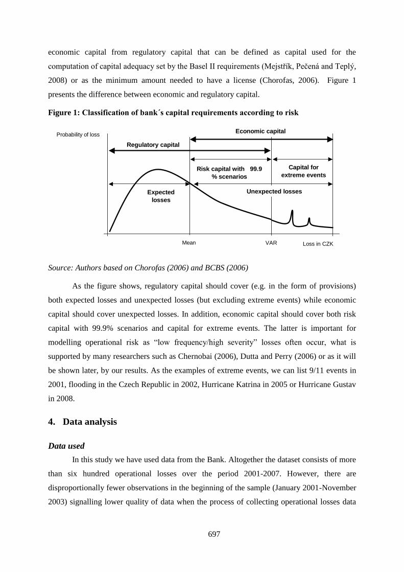
Figure 1: Classification of bank´s capital requirements according to risk

Source: Authors based on Chorofas (2006) and BCBS (2006)

As the figure shows, regulatory capital should cover (e.g. in the form of provisions)

both expected losses and unexpected losses (but excluding extreme events) while economic

capital should cover unexpected losses. In addition, economic capital should cover both risk

capital with 99.9% scenarios and capital for extreme events. The latter is important for

modelling operational risk as ―low frequency/high severity‖ losses often occur, what is

supported by many researchers such as Chernobai (2006), Dutta and Perry (2006) or as it will

be shown later, by our results. As the examples of extreme events, we can list 9/11 events in

2001, flooding in the Czech Republic in 2002, Hurricane Katrina in 2005 or Hurricane Gustav

in 2008.

4. Data analysis

Data used

In this study we have used data from the Bank. Altogether the dataset consists of more

than six hundred operational losses over the period 2001-2007. However, there are

disproportionally fewer observations in the beginning of the sample (January 2001-November

2003) signalling lower quality of data when the process of collecting operational losses data

Probability of loss

Loss in CZK

Regulatory capital

Economic capital

Risk capital with 99.9

% scenarios

Capital for

extreme events

Expected

losses

Unexpected losses

VARMean

698

was just starting. In order to remove possible bias, we have left out 14 observations of this

period.

Moreover, the threshold for collecting the data in the Bank (about $1,000) is set quite

low compared to other studies, the threshold is typically of the order of $10,000, hence we

further cut some of the observations from the beginning as we describe in the section dealing

with LDA. By setting the threshold up to $10,000 we have left out many small losses, hence

the number of observation in our dataset further decreased up to 23610

.

Observations across years starting from December 2004 are by a simple graphical

inspection quite stationary and hence can be considered to be collected by consistent

methodology. However, there is a significant variation across months; particularly losses in

December are significantly more frequent. This can be explained by the end of fiscal year

when all possible unrecorded losses up to a date finally appear on the books. This is not a

problem when losses are treated on annual basis or independent of time, however, it hinders

the possibility to take into account monthly information.

Generally, our dataset is not very big, but it is satisfactory enough for operational risk

analysis at the level of the whole bank. For analysis focusing on particular business lines

and/or particular type of loss events we would need more observations.

Exploratory data analysis

To get a better understanding of the structure and characteristics of the data we have

firstly performed Exploratory Data Analysis as suggested by Tukey (1977). Operational risk

data are skewed and heavy-tailed; hence skewness and kurtosis are the most important

characteristics. We have utilised some of the measures proposed by Hoaglin (1985) and

Tukey (1977) used in Dutta and Perry (2007) to analyse skewness and kurtosis. Employing

measures of skeweness such as a mid-summary plot or pseudo sigma indicator of excess

kurtosis, we confirmed that also our data are very skewed and heavy-tailed, the properties

typical for operational losses data11

.

10 Although the number of observations left out is high, they account only for about 2.5% of the sum of total

operational losses in the sample. A $10,000 threshold is commonly used in operational risk modelling (see Duta,

Perry (2007) or Chernobai (2007)). 11

For a more detailed analysis, please refer to Chalupka and Teplý (2008).

699

5. Methodology

5.1 Concept of VAR, modelling frequency and aggregation of losses

Before describing individual approaches to model operational risk, we would like to

define Value at Risk (VAR), a risk informative indicator recognised by Basel II

requirements.12

Jorion (2007) defines VAR as ―the maximum loss over a target horizon such

that there is a low, prespecified probability that the actual loss will be higher‖. Usually VAR

is expressed as a corresponding value (in currency units) of p% quantile of a distribution13

where p is the prespecified low probability and f(x) is a density function of operational losses:

VAR

dxxfp )(

(1)

Alternatively, VAR is a cut-off point of the distribution beyond which the probability

of the loss occurrence is less than p. For operational risk losses the quantile defined in Basel II

is 99.9% (see Chyba! Nenalezen zdroj odkazů.), thus we will report VAR99.9 for each

modelling method used. The target horizon is one year, so a 99.9% VAR requirement can be

interpreted as the maximum annual loss incurred over 1,000 years.

There is one complication associated with the above definition of VAR and the

requirement of Basel II. The above density function f(x) has to combine both the severity and

frequency of losses for a period of one year which is analytically difficult in specific cases

(Embrechts et al., 2005). One of the approaches suggested (e.g. Cruz, (2002), Embrechts et al.

(2005) or Dutta and Perry (2007)) is the Monte Carlo (MC) simulation where for a simulation

of a given year a number of losses is drawn from a frequency distribution and each loss in the

year is simulated by a random quantile of a severity distribution. All losses in each of the

simulated years are then summed to arrive at the estimation of the combined distribution

function. The 99.9% quantile is then taken from these simulated annual losses as the estimator

of the 99.9% VAR. We have simulated 10,000 years, however, as argued by Embrechts et al.

(2005) for rare events, the convergence of the MC estimator to the true values may not be

particularly fast, so in real applications either using more iterations or refining the standard

12 For more details on the VAR methodology see the traditional risk management books such as Jorion (2007),

Saunders and Cornett (2006) or Sironi and Resti (2007).

13 Although it is sometimes also defined as the difference between the mean and the quantile.

700

MC by importance sampling technique is suggested14

. To model frequency we have used

Poisson distribution, which is typically employed, having the density function

!)(

x

exf

x , (2)

and a single parameter λ. We have estimated it using three complete years 2004-2006

and for each year of the simulation we generated a random number of losses based on this

parameter. For EVT we have not modelled the whole distribution but rather the tail by

applying either the generalised extreme value (GEV) or the generalised Pareto distribution

(GPD). In these cases (following Dutta et al., 2007) we have used empirical sampling15

for the

body of the distribution. Hence, the VAR has been calculated by a MC simulation in which a

part of losses was drawn from the actual past losses and the other part was modelled by an

EVT model. The proportion of losses in the tail for the calculation of VAR was set to 2% as

this percentage of the highest losses appears to be the best to fit the data. The frequencies

were again modelled using the Poisson distribution.

5.2 Loss distribution approach

In the loss distribution approach (LDA) we have made use of a few parametric

distributions to try to model the whole distribution of the operational losses. As we have seen

in the exploratory data analysis, the empirical distribution of our data is highly skewed and

leptokurtotic, hence the distribution we have chosen allows for this. As the benchmark,

exponential distribution with only one parameter is utilised, secondly, three two-parameter

distributions (standard gamma, lognormal, and log-logistic) and the five-parameter

generalised hyperbolic (GH) distribution. GH distribution belongs into general class of

distributions and entails a wide range of other distributions and hence is more flexible for

modelling. For more details on this methodology we refer to Chalupka and Teply (2008),

P.D‘Agostino and Stephens (1986), Embrechts et al. (1997) or Hoaglin (1985).

5.3 Extreme value theory

Extreme value theory (EVT) is a promising class of approaches to modelling of

operational risk. Although originally utilised in other fields such as hydrology or non-life

14 Furthermore, the outlined aggregation of losses assumes that individual losses and the density function for

severity and frequency are independent; in the context of operational losses this is a reasonable assumption.

15 Empirical sampling – randomly drawing actual losses from the dataset.

701

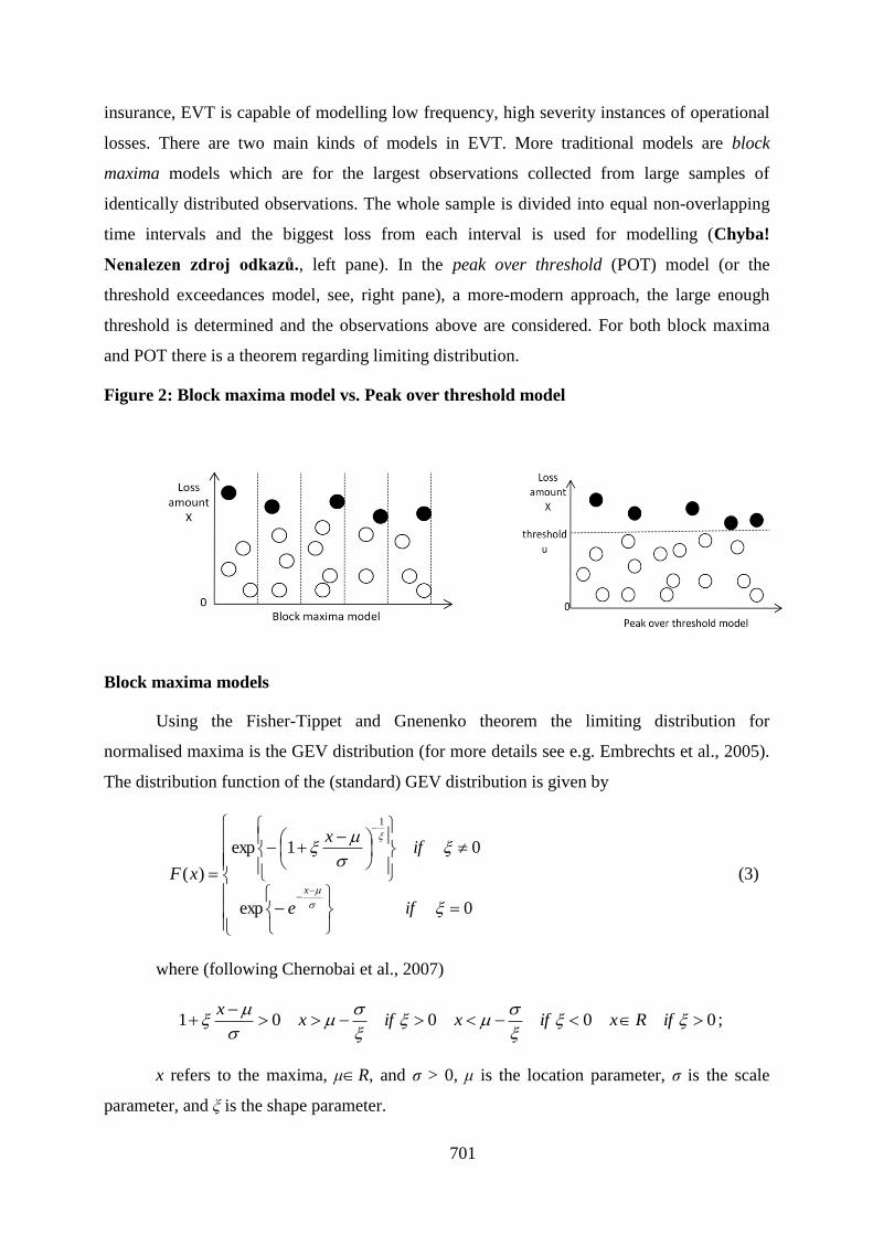
insurance, EVT is capable of modelling low frequency, high severity instances of operational

losses. There are two main kinds of models in EVT. More traditional models are block

maxima models which are for the largest observations collected from large samples of

identically distributed observations. The whole sample is divided into equal non-overlapping

time intervals and the biggest loss from each interval is used for modelling (Chyba!

Nenalezen zdroj odkazů., left pane). In the peak over threshold (POT) model (or the

threshold exceedances model, see, right pane), a more-modern approach, the large enough

threshold is determined and the observations above are considered. For both block maxima

and POT there is a theorem regarding limiting distribution.

Figure 2: Block maxima model vs. Peak over threshold model

Block maxima models

Using the Fisher-Tippet and Gnenenko theorem the limiting distribution for

normalised maxima is the GEV distribution (for more details see e.g. Embrechts et al., 2005).

The distribution function of the (standard) GEV distribution is given by

0exp

01exp

)(

1

ife

ifx

xFx

(3)

where (following Chernobai et al., 2007)

00001

ifRxifxifx

x;

x refers to the maxima, μR, and σ > 0, μ is the location parameter, σ is the scale

parameter, and ξ is the shape parameter.

702

The GEV distribution can be divided into three cases based on the value of the shape

parameter. For ξ > 0, the GEV is of the Fréchet case which is particularly suitable for

operational losses as the tail of the distribution is slowly varying (power decay), hence it is

able to account for high operational losses. It may be further shown that E(Xk)=∞ for k > 1/ξ,

thus for instance if ξ ≥ 1/2 a distribution has infinite variance and higher moments (Embrechts

et al., 1997).

The Gumbel case (ξ = 0) is also plausible for operational losses, although a tail is

decreasing faster (exponential decay), it has a heavier tail than the normal distribution. The

moments are always finite (E(Xk) < ∞ for k > 0). The Weibull case (ξ < 0) is of the least

importance as the right endpoint is finite, hence unable to model heavy tails of operational

losses. The GEV distribution can be fitted using various methods, we are going to describe

and use the two most commonly used, maximum likelihood and probability-weighted

moments. Denoting fξ,μ,σ the density of the GEV distribution, and M1,…,Mm being the block

maxima, the log-likelihood is calculated to be

m

i

m

i

im

i

ii

m

MMmMf

MMl

1 1

1

1

,,

1

1ln1ln1

1lnln

,,;,,

, (4)

which must be maximised subject to the parameter constraints that σ > 0 and

1 + ξ(Mi – μ)/σ > 0 for all i. (for more details see Embrechts et al., 2005).

Probability weighted moments (PWM), the second used approach to estimate

parameters of GEV, has better applicability to small samples than maximum likelihood (ML)

method (Landwehr et al., 1979). Following Hosking et al. (1985), although probability

weighted estimators are asymptotically inefficient compared to ML estimators, no deficiency

is detectable in samples of 100 or less. As the number of extreme observations is typically

limited, this property of PWM makes it very valuable in operational risk modelling.

Points over threshold models

As argued by Embrechts et al. (2005) block maxima models are very wasteful of data

as they consider only the highest losses in large blocks. Consequently, methods based on

threshold exceedances are used more frequently in practice. These methods utilise all data that

exceed a particular designated high level. Based on the Pickands-Balkema-de Haan theorem,

the limiting distribution of such points over thresholds (POT) is the GPD. For more details on

703

this methodology we refer to Chalupka and Teply (2008), Embrechts et al. (2005) or

Chernobai et al. (2007).

6. Empirical results

6.1 Loss distribution approach

As would be expected, the simple parametric distributions with one or 2-parameters

are far too simple to model operational loss data. Although moving from exponential to a

gamma distribution and from a gamma to a lognormal or a log-logistic somewhat improves

the fit, both QQ plots and the test statistics reject the hypothesis that the data follow any of

these distributions. The reason is that the losses in the end of the tail of the distribution are

significantly underpredicted.

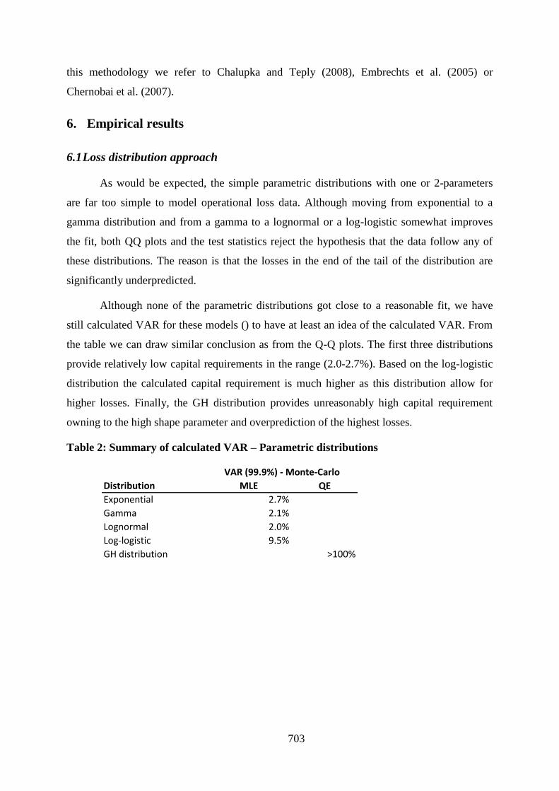
Although none of the parametric distributions got close to a reasonable fit, we have

still calculated VAR for these models () to have at least an idea of the calculated VAR. From

the table we can draw similar conclusion as from the Q-Q plots. The first three distributions

provide relatively low capital requirements in the range (2.0-2.7%). Based on the log-logistic

distribution the calculated capital requirement is much higher as this distribution allow for

higher losses. Finally, the GH distribution provides unreasonably high capital requirement

owning to the high shape parameter and overprediction of the highest losses.

Table 2: Summary of calculated VAR – Parametric distributions

MLE QE

Exponential 2.7%

Gamma 2.1%

Lognormal 2.0%

Log-logistic 9.5%

GH distribution >100%

Distribution

VAR (99.9%) - Monte-Carlo

704

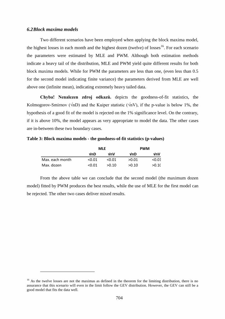
6.2 Block maxima models

Two different scenarios have been employed when applying the block maxima model,

the highest losses in each month and the highest dozen (twelve) of losses16

. For each scenario

the parameters were estimated by MLE and PWM. Although both estimation methods

indicate a heavy tail of the distribution, MLE and PWM yield quite different results for both

block maxima models. While for PWM the parameters are less than one, (even less than 0.5

for the second model indicating finite variance) the parameters derived from MLE are well

above one (infinite mean), indicating extremely heavy tailed data.

Chyba! Nenalezen zdroj odkazů. depicts the goodness-of-fit statistics, the

Kolmogorov-Smirnov (√nD) and the Kuiper statistic (√nV), if the p-value is below 1%, the

hypothesis of a good fit of the model is rejected on the 1% significance level. On the contrary,

if it is above 10%, the model appears as very appropriate to model the data. The other cases

are in-between these two boundary cases.

Table 3: Block maxima models - the goodness-of-fit statistics (p-values)

From the above table we can conclude that the second model (the maximum dozen

model) fitted by PWM produces the best results, while the use of MLE for the first model can

be rejected. The other two cases deliver mixed results.

16 As the twelve losses are not the maximas as defined in the theorem for the limiting distribution, there is no

assurance that this scenario will even in the limit follow the GEV distribution. However, the GEV can still be a

good model that fits the data well.

√nD √nV √nD √nV

Max. each month <0.01 <0.01 >0.01 <0.01

Max. dozen <0.01 >0.10 >0.10 >0.10

MLE PWM

705

Figure 3: Block maxima model – QQ-plot for max. dozen model fitted by PWM

The QQ-plot above shows that although the maximum dozen model estimated by

PWM slightly underpredicts the highest losses, the fit of the data is very good, supporting the

adequacy of this model.

Points over threshold models

We have chosen four different models. Firstly, using the excess plot we have

identified a threshold (Figure 4Chyba! Nenalezen zdroj odkazů.). The plot is reasonably

linear over the given range; the threshold is set at the level of a small ―kink‖ where the slope

decreases slightly17

. This threshold is slightly higher than 10% of all losses in the data set.

Additionally, we have used 2%, 5% and 10% of the highest losses.

Figure 4: POT model – Mean excess plot

17 Slightly above 0.04 on the virtual horizontal axis.

0

1

2

3

4

5

0 1 2 3 4 5

pre

dic

ted

loss

es

actual losses

Block maxima - max. dozen (PWM)

0.00

0.10

0.20

0.30

0.40

0.50

0.60

0.70

0.00 0.02 0.04 0.06 0.08 0.10

Me

an e

xce

ss

Threshold

Mean excess plot

706

Again, the shape parameter obtained from different methods differs significantly

(Table 4). However, we can trace some consistency at least from the PWM results. As noted

by Embrechts (2005) the shape parameter of the limiting GPD for the excesses is the same as

the shape parameter of the limiting GEV distribution for the maxima. Indeed, for our data,

the block maxima model of maximum dozen losses (approximately 2% of losses) is close to

the threshold of 2% highest losses from the POT model. Additionally, the other three POT

models have the shape estimates close to each other.

Table 4: Threshold exceedances models - the shape parameter

Regarding the goodness-of-fit, the outcomes (Table 5) are generally plausible for both

estimation methods. Therefore, we can conclude, that the models appear reasonable from the

statistical point of view, what is also supported by the QQ-plot, which exhibits the best visual

fit and at the same time displays consistency with the block maxima model.

Table 5: Threshold exceedances models - the goodness-of-fit statistics (p-values)

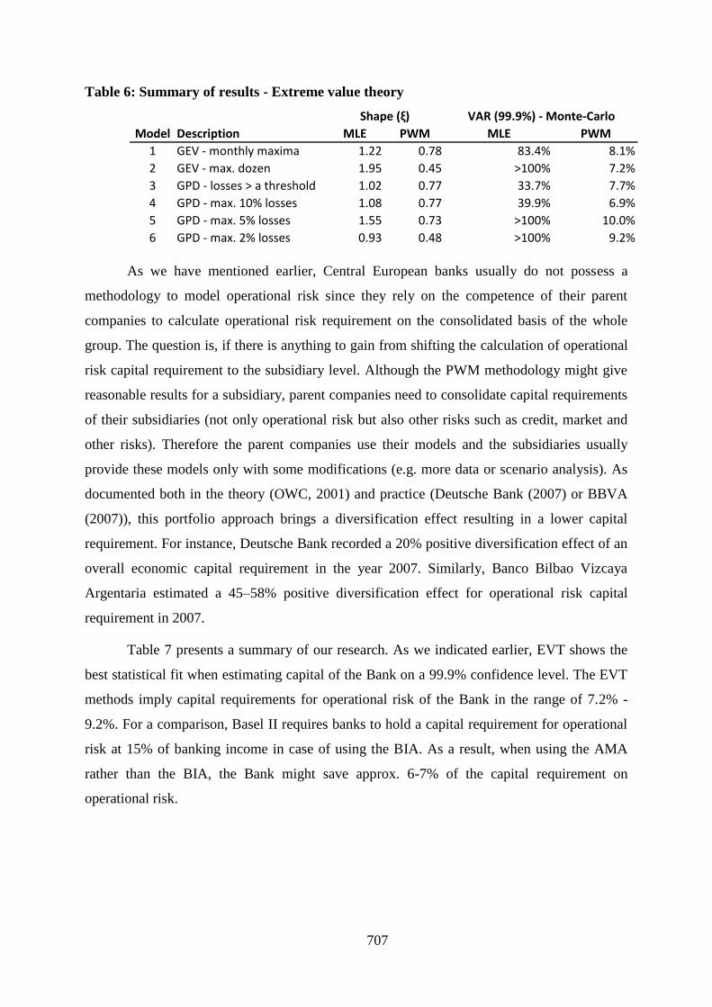
6.3 Summary of results

The Table 6 summarises the result for EVT. The high shape parameters for some of

the models estimated by MLE result in unreasonable high capital estimates, higher than 100%

of the corresponding bank income. On the other hand, capital estimates by PWM are quite

consistent from a practical point of view, ranging from 6.9%–10.0%, indicating alongside

with the arguments already mentioned that this method might be more suitable in the

estimation of operational risk when the data are limited.

MLE PWM

Losses > a threshold 1.02 0.77

Max. 10% losses 1.08 0.77

Max. 5% losses 1.55 0.73

Max. 2 % losses 0.93 0.48

√nD √nV √nD √nV

Losses > a threshold >0.10 >0.05 >0.01 >0.05

Max. 10% losses >0.10 >0.10 >0.01 >0.10

Max. 5% losses >0.10 >0.10 <0.01 >0.025

Max. 2 % losses >0.10 >0.10 >0.10 >0.10

MLE PWM

707

Table 6: Summary of results - Extreme value theory

As we have mentioned earlier, Central European banks usually do not possess a

methodology to model operational risk since they rely on the competence of their parent

companies to calculate operational risk requirement on the consolidated basis of the whole

group. The question is, if there is anything to gain from shifting the calculation of operational

risk capital requirement to the subsidiary level. Although the PWM methodology might give

reasonable results for a subsidiary, parent companies need to consolidate capital requirements

of their subsidiaries (not only operational risk but also other risks such as credit, market and

other risks). Therefore the parent companies use their models and the subsidiaries usually

provide these models only with some modifications (e.g. more data or scenario analysis). As

documented both in the theory (OWC, 2001) and practice (Deutsche Bank (2007) or BBVA

(2007)), this portfolio approach brings a diversification effect resulting in a lower capital

requirement. For instance, Deutsche Bank recorded a 20% positive diversification effect of an

overall economic capital requirement in the year 2007. Similarly, Banco Bilbao Vizcaya

Argentaria estimated a 45–58% positive diversification effect for operational risk capital

requirement in 2007.

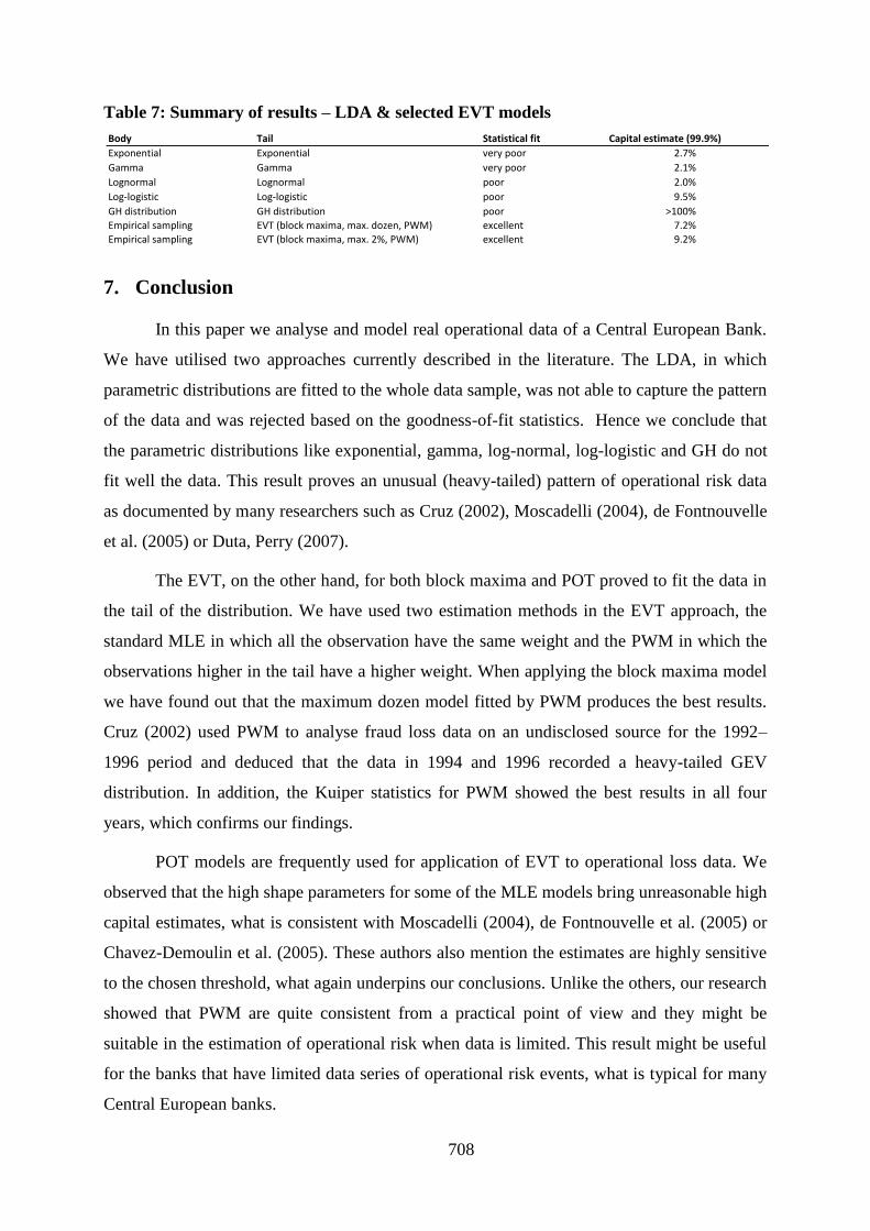
Table 7 presents a summary of our research. As we indicated earlier, EVT shows the

best statistical fit when estimating capital of the Bank on a 99.9% confidence level. The EVT

methods imply capital requirements for operational risk of the Bank in the range of 7.2% -

9.2%. For a comparison, Basel II requires banks to hold a capital requirement for operational

risk at 15% of banking income in case of using the BIA. As a result, when using the AMA

rather than the BIA, the Bank might save approx. 6-7% of the capital requirement on

operational risk.

MLE PWM MLE PWM

1 GEV - monthly maxima 1.22 0.78 83.4% 8.1%

2 GEV - max. dozen 1.95 0.45 >100% 7.2%

3 GPD - losses > a threshold 1.02 0.77 33.7% 7.7%

4 GPD - max. 10% losses 1.08 0.77 39.9% 6.9%

5 GPD - max. 5% losses 1.55 0.73 >100% 10.0%

6 GPD - max. 2% losses 0.93 0.48 >100% 9.2%

Model Description

Shape (ξ) VAR (99.9%) - Monte-Carlo

708

Table 7: Summary of results – LDA & selected EVT models

7. Conclusion

In this paper we analyse and model real operational data of a Central European Bank.

We have utilised two approaches currently described in the literature. The LDA, in which

parametric distributions are fitted to the whole data sample, was not able to capture the pattern

of the data and was rejected based on the goodness-of-fit statistics. Hence we conclude that

the parametric distributions like exponential, gamma, log-normal, log-logistic and GH do not

fit well the data. This result proves an unusual (heavy-tailed) pattern of operational risk data

as documented by many researchers such as Cruz (2002), Moscadelli (2004), de Fontnouvelle

et al. (2005) or Duta, Perry (2007).

The EVT, on the other hand, for both block maxima and POT proved to fit the data in

the tail of the distribution. We have used two estimation methods in the EVT approach, the

standard MLE in which all the observation have the same weight and the PWM in which the

observations higher in the tail have a higher weight. When applying the block maxima model

we have found out that the maximum dozen model fitted by PWM produces the best results.

Cruz (2002) used PWM to analyse fraud loss data on an undisclosed source for the 1992–

1996 period and deduced that the data in 1994 and 1996 recorded a heavy-tailed GEV

distribution. In addition, the Kuiper statistics for PWM showed the best results in all four

years, which confirms our findings.

POT models are frequently used for application of EVT to operational loss data. We

observed that the high shape parameters for some of the MLE models bring unreasonable high

capital estimates, what is consistent with Moscadelli (2004), de Fontnouvelle et al. (2005) or

Chavez-Demoulin et al. (2005). These authors also mention the estimates are highly sensitive

to the chosen threshold, what again underpins our conclusions. Unlike the others, our research

showed that PWM are quite consistent from a practical point of view and they might be

suitable in the estimation of operational risk when data is limited. This result might be useful

for the banks that have limited data series of operational risk events, what is typical for many

Central European banks.

Body Tail Statistical fit Capital estimate (99.9%)

Exponential Exponential very poor 2.7%

Gamma Gamma very poor 2.1%

Lognormal Lognormal poor 2.0%

Log-logistic Log-logistic poor 9.5%

GH distribution GH distribution poor >100%

Empirical sampling EVT (block maxima, max. dozen, PWM) excellent 7.2%

Empirical sampling EVT (block maxima, max. 2%, PWM) excellent 9.2%

709

From a policy perspective it should be hence noted that banks from emerging markets

such as the Central Europe are also able to register operational risk events. Data from the

Bank showed an improvement in time, what could be attributed to more attention devoted to

recording operational risk events. Moreover, as we have demonstrated, the distribution of

these risk events can be estimated with a similar success than those from more mature

markets.

Despite the conclusions cited above, there are still several ways in which our research

can be improved. Firstly, a similar study can be done on a larger sample of data (we used the

data from one Central European bank). Secondly, the research provided on all eight business

lines recognised by Basel II may reveal interesting facts about different operational risk

features among various business lines. Finally, other research might include other results

derives from modelling operational risk using such techniques as robust statistics, stress-

testing, Bayesian inference, dynamic Bayesian networks and expectation maximisation

algorithms.

References

[1] ARAI, T. Key points of scenario analysis. Bank of Japan, 2006.

[2] BBVA. Banco Bilbao Vizcaya Argentaria. Annual Report 2007, 2007.

[3] BCBS. International Convergence of Capital Measurement and Capital Standards, A

Revised Framework, Comprehensive Version. Basel Committee on Banking

Supervision, Bank for International Settlement, Basel, 2006.

[4] BEE, M.: Estimating and simulating loss distributions with incomplete data, Oprisk and

Compliance; 7 (7): 38-41, 2006.

[5] CHALUPKA, R. and TEPLY, P. Operational Risk and Implications for Economic

Capital – A Case Study, IES Working paper 17/2008, IES FSV, Charles University,

Czech Republic, 2008.

[6] CHERNOBAI, A.S., RACHEV, S.T. and FABOZZI, F.J. Operational Risk: A Guide to

Basel II Capital Requirements, Models, and Analysis. John Wiley & Sons, Inc., 2007.

[7] CHOROFAS, D. Economic Capital Allocation with Basel II. Elsevier, Oxford, 2006.

[8] CRUZ, M., COLEMAN, R. and GERRY, S. Modeling and Measuring Operational Risk.

Journal of Risk, Vol. 1, No. 1: 63–72, 1998.

710

[9] CRUZ, M.G. Modeling, Measuring and Hedging Operational Risk, John Wiley & Sons,

Ltd., 2002.

[10] DE FONTNOUVELLE, P., DE JESUS-RUEFF, V., JORDAN, J., ROSENGREN, E.

Using Loss Data to Quantify Operational Risk. Technical report, Federal Reserve Bank

of Boston and Fitch Risk, 2003.

[11] DE FONTNOUVELLE, P., JORDAN, J. and ROSENGREN, E. Implications of

Alternative Operational Risk Modeling Techniques. NBER Working Paper No. W11103,

2005.

[12] DEUTSCHE BANK. Deutsche Bank, Annual Report 2007, 2007.

[13] DILLEY, B. Mortgage fraud getting serious. Frontiers in Finance, KPMG, July 2008

[14] DUTTA, K. and PERRY, J. A tale of tails: An empirical analysis of loss distribution

models for estimating operational risk capital. Federal Reserve Bank of Boston,

Working Papers No. 06-13, 2007.

[15] EMBRECHTS, P., DEGEN, M. and LAMBRIGGER, D. The quantitative modelling of

operational risk: between g-and-h and EVT. Technical Report ETH Zurich, 2002.

[16] EMBRECHTS, P., FURRER, H. and KAUFMANN, R. Quantifying regulatory capital

for operational risk. Derivatives Use, Trading & Regulation, 9 (3): 217–223, 2003.

[17] EMBRECHTS, P, KAUFMANN R, SAMORODNITSKY, G. Ruin Theory Revisited:

Stochastic Models for Operational Risk. Working Paper, ETH-Zurich and Cornell

University, 2002.

[18] EMBRECHTS, P., KLÜPPELBERG, C. and MIKOSCH, T. Modelling Extremal Events

for Insurance and Finance. Springer, 1997.

[19] EMBRECHTS, P., MCNEIL, A. and RUDIGER, F. Quantitative Risk Management,

Techniques and Tools. Princeton Series in Finance, 2005.

[20] FITCH RATINGS. Operational Risk Grapevine, Fitch Ratings, March 2007

[21] HIWATSHI, J. and ASHIDA, H. advancing Operational Risk Management Using

Japanese Banking Experiences. Technical report, Federal Reserve Bank of Chicago,

2002.

[22] HOAGLIN, D.C., MOSTELLER, F., TUKEY, J.W. Exploring Data Tables, Trends,

and Shapes, New York, NY: John Wiley & Sons, Inc., 1985.

711

[23] HOSKING, J.R.M., WALLIS, J.R. and WOOD, E. Estimation of Generalized Extreme

Value Distribution by the Method of Probability Weighted Moments, Technometrics,

27: 251-261, 1985.

[24] HOSKING, J.R.M. and WALLIS, J.R. Regional Frequency Analysis: an approach

based on moments. Cambridge University Press, Cambridge, UK, 1997.

[25] JOBST, A.A. Operational Risk — The Sting is Still in the Tail but the Poison Depends

on the Dose. IMF Working paper 07/239, International Monetary Fund, 2007b.

[26] JOBST, A.A. The Regulation of Operational Risk under the New Basel Capital Accord -

Critical Issues. International Journal of Banking Law and Regulation, Vol. 21, No. 5:

249–73, 2007c.

[27] JORION, P. Value at Risk: The New Benchmark for Managing Financial Risk. 2nd

edition, McGraw-Hill, New York, 2000.

[28] JORION, P. Financial Risk Manager Handbook. Wiley Finance, 2007.

[29] KING, J.L. Operational Risk: Measuring and Modelling. John Wiley & Sons, New

York, 2001.

[30] LAWRENCE, M. Marking the Cards at Anz, Operational Risk Supplement. Risk

Publishing, London, UK, 2000. 5-8

[31] MEJSTŘÍK, M., PEČENÁ, M. and TEPLÝ, P. Basic Principles of Banking. Karolinum

Press, Prague, 2008.

[32] MOSCADELLI, M. The modelling of operational risk: experience with analysis of the

data, collected by the Basel Committee. Banca d‘Italia, Temi di discussion del Servizio

Studi, No. 517–July, 2004.

[33] OWC. Study on the Risk Profile and Capital Adequacy of Financial Conglomerates,

London: Oliver, Wyman and Company, 2001.

[34] NEŠLEHOVÁ, J., EMBRECHTS, P. and CHAVEZ-DEMOULIN, V. Infinite Mean

Models and the LDA for Operational Risk. Journal of Operational Risk, Vol. 1, No. 1:

3–25, 2006.

[35] PANJER, H. Operational Risk: Modeling Analytics. Wiley, 2006.

[36] POWER, M. The invention of operational risk. Review of International Political

Economy, October 2005: 577–599, 2005.

712

[37] RIPPEL, M. and TEPLÝ, P. Operational Risk - Scenario Analysis. IES Working paper

15/2008, Charles University, Czech Republic, 2008.

[38] ROSENGREN, E. Scenario analysis and the AMA, Federal Reserve Bank of Boston,

2006.

[39] SAUNDERS, A., CORNETT, M.M. Financial Institutions Management. 5th edition,

McGraw-Hill/Irwin, 2006.

[40] SHEVCHENKO, P. and WUTHRICH, M. The structural modelling of operational risk

via Bayesian inference: Combining loss data with expert opinions. CSIRO Technical

Report Series, CMIS Call Number 2371, 2006.

[41] SIRONI, A. and RESTI, A. Risk Management and Shareholders’ Value in Banking, 1st

edition, Wiley, 2007.

[42] TUKEY, J.W. Exploratory Data Analysis, Reading. MA: Addison-Wesley, 1977

[43] VAN DEN BRINK, J. Operational Risk: The New Challenge for Banks. Palgrave,

London, 2002.

[44] VAN LEYVELD, P et al. Economic Capital Modelling: Concepts, Measurement and

Implementation. Laurie Donaldson, London, 2006.

[45] TEPLY, P., CERNOHORSKY, J., CERNOHORSKA, L. Strategic Implications of The

2008 Financial Crisis, Global Strategic Management, Inc., Michigan, USA, ISSN 1947-

2195, 2009.

[46] TEPLY, P. Three essays on risk management and financial stability. Dissertation

thesis, 2009, Charles University in Prague, Czech Republic