1

The (in)Completeness of the Observed InternetAS-level Structure

Ricardo Oliveira∗ Dan Pei† Walter Willinger † Beichuan Zhang ‡ Lixia Zhang∗

∗{rveloso,lixia}@cs.ucla.edu †{peidan,walter}@research.att.com ‡bzhang@arizona.eduUniversity of California, Los Angeles AT&T Labs – Research University of Arizona

Abstract— Despite significant efforts to obtain an accuratepicture of the Internet’s connectivity structure at the levelof individual autonomous systems (ASes), much has remainedunknown in terms of the quality of the inferred AS maps thathave been widely used by the research community. In this paperwe assess the quality of the inferred Internet maps through casestudies of a sample set of ASes. These case studies allow usto establish the ground truth of connectivity between this set ofASes and their directly connected neighbors. A direct comparisonbetween the ground truth and inferred topology maps yieldinsights into questions such as which parts of the actual topologyare adequately captured by the inferred maps, which parts aremissing and why, and what is the percentage of missing links inthese parts. This information is critical in assessing, for eachclass of real-world networking problems, whether the use ofcurrently inferred AS maps or proposed AS topology modelsis, or is not, appropriate. More importantly, our newly gainedinsights also point to new directions towards building realisticand economically viable Internet topology maps.

I. INTRODUCTION

Many research projects have used a graphic representationof the Internet topology, where nodes represent autonomoussystems (ASes) and two nodes are connected if and only if thetwo ASes are engaged in a business relationship to exchangedata traffic. Due to the Internet’s decentralized architecture,however, this AS-level construct is not readily available andobtaining accurate AS maps has remained an active areaof research. All the AS maps that have been used by theresearch community have been inferred from either BGP-based or traceroute-based data. Unfortunately, both types ofmeasurements are more a reflection of what we can measurethan what we want to measure, as both have fundamentallimitations in their ability to reveal the Internet’s true AS-levelconnectivity structure.

While these limitations inherent in the available data havelong been recognized, there has been little effort in assessingthe degree of completeness or accuracy of the resulting ASmaps. Although it is relatively easy to collect a more or lesscomplete set of ASes, it has proven difficult, if not impossible,to collect the complete set of inter-AS links. The sheer scaleof the Internet makes it infeasible to either install monitorseverywhere or crawl the topology exhaustively. At the sametime, big stakeholders of the AS-level Internet, such as Internetservice providers and large content providers, tend to viewtheir AS connectivity as proprietary information and are in

general unwilling to disclose it. As a result, the quality of thecurrently used AS maps has remained by and large unknown.Yet numerous projects have been conducted using these mapsof unknown quality, causing serious scientific and practicalconcerns in terms of the validity of the claims made andaccuracy of the results reported.

In this paper we take a first step towards a rigorous as-sessment of the quality of the Internet’s AS-level connectivitymaps inferred from public BGP data. Realizing the futility ofattempting to obtain the complete global AS-level topology,we take an indirect approach to address the problem. Using asmall number of different types of ASes whose complete ASconnectivity information can be obtained, we conduct casestudies to compare their actual connectivity with that of whatwe call the “public view” – the connectivity structure inferredfrom all the publicly available and commonly-used BGPdata source (i.e., routing tables, updates, looking glasses, androuting registry). These case studies enable us to understandand verify what kinds of AS links are adequately capturedby the public view and what kinds of (and how many) ASlinks are missing from the public view. They also providenew insights into where the missing links are located withinthe overall AS topology.

More specifically, this paper makes the following originalcontributions. After we define what we mean by “ground truth”of AS-level Internet connectivity between a single AS and itsneighbors in Section II, we report in Section III on a series ofcase studies which highlight the difficulties in establishing theground truth, namely the data sources necessary to establishthe AS-level connectivity are not publicly available for mostASes. Nevertheless, by classifying ASes into a few majortypes, we can explore what types and what fraction of eachtype of AS connectivity are missing from currently used ASmaps, and we can typically identify the reasons why they aremissing.

The main findings of our search for the elusive groundtruth of AS-level Internet connectivity can be summarized asfollows. First, inferred AS maps based on single snapshotsof publicly available BGP-based data are typically of lowquality. The percentage of missing links can range from 10-20% for Tier-1 and Tier-2 ASes to 85% or more for largecontent networks. Second, the quality of the inferred AS mapscan be significantly improved by including historic data ofBGP updates from all existing sources. For example, links

2

on backup paths can be revealed by routing dynamics overtime, but the time period required to collect the necessaryinformation can be several years. Third, through the use ofdata collected over long enough time periods, the publicview captures all the links of Tier-1 ASes and almost all thecustomer-provider links at all tiers in the Internet. Fourth, dueto the no-valley routing policy and the lack of monitors in moststub networks, the public view misses a great number of peerlinks at all tiers except tier-1. It may miss up to 90% of peerlinks in the case of large content provider networks, whichhave been aggressively adding peer links in recent years.

The paper concludes with a discussion in Section V onseveral main lessons learned from our case studies, a briefreview of related work in Section VI, and a summary detailingour future research plans in Section VII.

II. SEARCHING FOR THE GROUND TRUTH

This section gives a brief background on inter-domainnetwork connectivity, defines its ground truth, describes thevarious data sets and methods that we used to infer the inter-domain connectivity.

A. Inter-domain Connectivity and Peering

As of summer 2008, the Internet consists of more than27,000 networks called “Autonomous Systems” (AS). EachAS is represented by a unique numeric AS number and mayadvertise one or more IP address prefixes. ASes run the BorderGateway Protocol (BGP) [35] to propagate prefix reachabilityinformation among themselves. In the rest of the paper, wecall the connection between two ASes an AS link or simplya link. As a path-vector protocol, BGP includes in its routingupdates the entire AS-level path to each prefix, which canbe used to infer the AS-level connectivity. Projects suchas RouteViews [12] and RIPE-RIS [11] host multiple datacollectors that establish BGP sessions with operational routers,which we term monitors, in hundreds of ASes to obtain theirBGP forwarding tables and routing updates over time. BGProuting decisions are largely based on routing polices, inwhich the most important factor is the business relationshipbetween neighboring ASes. Though the relationship can befine-grained, in general there are three major types: customer-provider, peer-peer and sibling-sibling. In a customer-providerrelationship, the customer pays the provider for transitingtraffic from and to the rest of the Internet, thus the providerusually announces all the routes to the customer. In a peer-peerrelationship, which is commonly described as “settlement-free,” the two ASes exchange traffic without paying each other.However only the traffic originated from and destined to thetwo peering ASes or their downstream customers is allowedon a peer-peer link; traffic from their providers or other peersare not allowed. Therefore an AS does not announce routescontaining peer-peer links to its providers or other peers. Whenan AS receives path announcements to the same destinationfrom multiple neighbors, in general the AS prefers the pathannounced by a customer over that from a peer, and prefersa path from a peer over that from a provider. This is referredto as the no-valley-and-prefer-customer policy [22], which

is believed to be a common practice in today’s Internet. Thesibling-sibling relationship is between two ASes that belongto the same organization, and is relatively rare; thus we do notconsider it in this paper.

Among all the ASes, less than 10% are transit networks, andthe rest are stub networks. A transit network is an InternetService Provider (ISP) whose business is to provide packetforwarding service between other networks. Stub networks, onthe other hand, do not forward packets for other networks. Inthe global routing hierarchy, stub networks are at the bottomor at the edge, and need transit networks as their providersto reach the rest of the Internet. Transit networks may havetheir own providers and peers, and are usually described asdifferent tiers, e.g., regional ISPs, national ISPs, and globalISPs. At the top of this hierarchy are a dozen or so tier-1ISPs, which connect to each other in a fully mesh to form thecore of the global routing infrastructure. The majority of stubnetworks today multi-home with more than one provider, andsome stub networks also peer with each other. In particular,content networks, e.g., networks supporting search engines, e-commerce, and social network sites, tend to peer with a largenumber of other networks.

Peering is a delicate but also important issue in inter-domainconnectivity. A network has incentives to peer with other net-works to reduce the traffic sent to its providers, hence savingoperational costs. But peering also comes with its own issues.For ISPs, besides additional equipment and management cost,they also do not want to establish peer-peer relationshipswith potential customers. Therefore ISPs in general are veryselective in choosing their peers. Common criteria includenumber of co-locations, ratio of inbound and outbound traffic,and certain requirements on prefix announcements [2], [1].In recent years, with the fast growth of available content inthe Internet, content networks have been keen on peering withother networks to bypass their providers. Because they have noconcern regarding transit traffic or potential customers, contentnetworks generally have an open peering policy and peer witha large number of other networks.

AS peering can be realized through either private peering orpublic peering. A private peering is a dedicated connection be-tween two networks. It provides dedicated bandwidth, makestroubleshooting easier, but has a higher cost. Public peeringusually happens at the Internet Exchange Points (IXPs), whichare third-party maintained physical infrastructures that enablephysical connectivity between their member networks1. Cur-rently most IXPs connect their members through a sharedlayer-2 switching fabric (or layer-2 cloud). Figure 1 showsan IXP that interconnects ASes A through G using a subnet195.69.144.0/24. Though an IXP provides physical connec-tivity among all participants, it is up to individual networksto decide with whom to establish BGP sessions. It is oftenthe case that one network only peers with some of the otherparticipants in the same IXP. Public peering has a lower costbut its available bandwidth capacity between any two partiescan be limited. However, with the recent increase in bandwidth

1Note that private and public peering can happen in the same physicalfacility.

3

FC

D E

G

A

B

Layer-2 cloud

IXP

195.69.144.1

195.69.144.2195.69.144.7

195.69.144.3

195.69.144.4195.69.144.5

195.69.144.6

Fig. 1. A sample IXP. ASes A through G connectto each other through a layer-2 switch in subnet195.69.144/24.

5

2

4

1

9

6 7

83

10

Provider CostumerPeer Peer

Best path

(a) (b)

p0 p1 p2

Fig. 2. A set of interconnected ASes, each noderepresent an AS. (a) shows an example of hiddenLinks, and (b) an example of invisible Links.

10

20

129.213.1.1

129.213.1.2

BGP multihop

30

R0

R1

R2

R3

129.213.2.1

175.220.1.2

Fig. 3. Configuring remote BGP peerings. R0 andR2 are physically directly connected, while R1 andR3 are not.

capacity, we have seen a trend to migrate private peerings topublic peerings.

B. Ground Truth vs. Observed Map

To study AS-level connectivity, we need a clear definitionon what constitutes an inter-AS link. A link between twoASes exists if the two ASes have a contractual agreementto exchange traffic over one or multiple BGP sessions. Theground truth of the Internet AS-level connectivity is thecomplete set of AS links. As the Internet evolves, its AS-levelconnectivity also changes over time. We use Greal(t) to denotethe ground truth of the entire Internet AS-level connectivity attime t.

Ideally if each ISP maintains an up-to-date list of its ASlinks and makes the list accessible, obtaining the groundtruth would be trivial. However, such a list is proprietary andrarely available, especially for large ISPs with a large andchanging set of links. In this paper, we derive the ground truthof several individual networks whose data is made availableto us, including their router configurations, syslogs, BGPcommand outputs, as well as personal communications withthe operators.

From router configurations, syslogs and BGP commandoutputs, we can infer whether there is a working BGP session,i.e., a BGP session that is in the established state as specifiedin RFC 4271 [35]. We assume there is a link between twoASes if there is at least one working BGP session betweenthem. However if all the BGP sessions between two ASesare down at the moment of data collection, the link maynot appear in the ground truth on that particular day, eventhough the two ASes have a valid agreement to exchangetraffic. Fortunately we have continuous daily data going backfor years, thus the problem of missing links due to transientfailures should be negligible. When inferring connectivity fromrouter configurations, extra care is needed to remove stale BGPsessions, i.e. , sessions that appear to be correctly configuredin router configurations, but are actually no longer active. Weuse syslog data in this case to remove the stale entries (asdescribed in detail in the next section). We believe that thiscareful filtering makes our inferred connectivity a very goodapproximation of the real ground-truth.

We denote an observed global AS topology at time t byGobsv(t), which typically provides only a partial view of theground truth. There are two types of missing links when we

compare Gobsv and Greal: hidden links and invisible links.Given a set of monitors, a hidden link is one that has not yetbeen observed but could possibly be revealed at a later time.An invisible link is one that is impossible to be observed by thegiven set of monitors. For example, in Figure 2(a), assumingthat AS5 hosts a monitor (either a BGP monitoring router ora traceroute probing host) which sends to the collector all theAS paths used by AS5. Between the two customer paths toreach prefix p0, AS5 picks the best one, [5-2-1], so we are ableto observe the existence of AS links 2-1 and 5-2. The threeother links, 5-4, 4-3, and 3-1, are hidden at the time, but will berevealed when AS5 switches to path [5-4-3-1] if a failure alongthe primary path [5-2-1] occurs. In Figure 2(b), the monitorAS10 uses paths [10-8-6] and [10-9-7] to reach prefixes p1

and p2, respectively. In this case, link 8-9 is invisible to themonitor in AS10, because it is a peer link that will not beannounced to AS10 under any circumstances due to the no-valley policy.

Hidden links are typically revealed if we build AS mapsusing routing data (e.g., BGP updates) collected over anextended period. However, a new problem arises from thisapproach: the introduction of potentially stale links; that is,links that existed some time ago but are no longer present. Aempirical solution for removing possible stale links has beendeveloped in [33]. To discover all invisible links, we wouldneed additional monitors at most, if not all, edge ASes whererouting updates can contain the peering links as permitted byrouting policy. The issues of hidden and invisible links areshared by both BGP logs and traceroute measurements.

C. Data SetsWe use the following data sources to infer the AS-level

connectivity and the ground truth of individual ASes.BGP data: The public view (PV) of the AS-level con-

nectivity is derived from all public BGP data at our disposal.These data include BGP forwarding tables and updates from∼700 routers in ∼400 ASes provided by Routeviews, RIPE-RIS, Abilene [14], and the China Education and ResearchNetwork [3], BGP routing tables extracted from ∼80 routeservers, and “show ip bgp sum” outputs from ∼150 lookingglasses located worldwide. In addition, we use “show ip bgp”outputs from Abilene and Geant [5] to infer their ground truth.Note that we currently do not use AS topological data derivedfrom traceroute measurements due to issues in converting

4

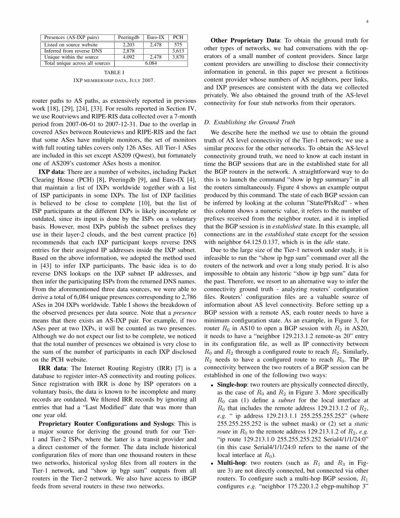
Presences (AS-IXP pairs) Peeringdb Euro-IX PCHListed on source website 2,203 2,478 575Inferred from reverse DNS 2,878 3,613Unique within the source 4,092 2,478 3,870Total unique across all sources 6,084

TABLE IIXP MEMBERSHIP DATA, JULY 2007.

router paths to AS paths, as extensively reported in previouswork [18], [29], [24], [33]. For results reported in Section IV,we use Routviews and RIPE-RIS data collected over a 7-monthperiod from 2007-06-01 to 2007-12-31. Due to the overlap incovered ASes between Routeviews and RIPE-RIS and the factthat some ASes have multiple monitors, the set of monitorswith full routing tables covers only 126 ASes. All Tier-1 ASesare included in this set except AS209 (Qwest), but fortunatelyone of AS209’s customer ASes hosts a monitor.

IXP data: There are a number of websites, including PacketClearing House (PCH) [8], Peeringdb [9], and Euro-IX [4],that maintain a list of IXPs worldwide together with a listof ISP participants in some IXPs. The list of IXP facilitiesis believed to be close to complete [10], but the list ofISP participants at the different IXPs is likely incomplete oroutdated, since its input is done by the ISPs on a voluntarybasis. However, most IXPs publish the subnet prefixes theyuse in their layer-2 clouds, and the best current practice [6]recommends that each IXP participant keeps reverse DNSentries for their assigned IP addresses inside the IXP subnet.Based on the above information, we adopted the method usedin [43] to infer IXP participants. The basic idea is to doreverse DNS lookups on the IXP subnet IP addresses, andthen infer the participating ISPs from the returned DNS names.From the aforementioned three data sources, we were able toderive a total of 6,084 unique presences corresponding to 2,786ASes in 204 IXPs worldwide. Table I shows the breakdown ofthe observed presences per data source. Note that a presencemeans that there exists an AS-IXP pair. For example, if twoASes peer at two IXPs, it will be counted as two presences.Although we do not expect our list to be complete, we noticedthat the total number of presences we obtained is very close tothe sum of the number of participants in each IXP disclosedon the PCH website.

IRR data: The Internet Routing Registry (IRR) [7] is adatabase to register inter-AS connectivity and routing polices.Since registration with IRR is done by ISP operators on avoluntary basis, the data is known to be incomplete and manyrecords are outdated. We filtered IRR records by ignoring allentries that had a “Last Modified” date that was more thanone year old.

Proprietary Router Configurations and Syslogs: This isa major source for deriving the ground truth for our Tier-1 and Tier-2 ISPs, where the latter is a transit provider anda direct customer of the former. The data include historicalconfiguration files of more than one thousand routers in thesetwo networks, historical syslog files from all routers in theTier-1 network, and “show ip bgp sum” outputs from allrouters in the Tier-2 network. We also have access to iBGPfeeds from several routers in these two networks.

Other Proprietary Data: To obtain the ground truth forother types of networks, we had conversations with the op-erators of a small number of content providers. Since largecontent providers are unwilling to disclose their connectivityinformation in general, in this paper we present a fictitiouscontent provider whose numbers of AS neighbors, peer links,and IXP presences are consistent with the data we collectedprivately. We also obtained the ground truth of the AS-levelconnectivity for four stub networks from their operators.

D. Establishing the Ground Truth

We describe here the method we use to obtain the groundtruth of AS level connectivity of the Tier-1 network; we use asimilar process for the other networks. To obtain the AS-levelconnectivity ground truth, we need to know at each instant intime the BGP sessions that are in the established state for allthe BGP routers in the network. A straightforward way to dothis is to launch the command “show ip bgp summary” in allthe routers simultaneously. Figure 4 shows an example outputproduced by this command. The state of each BGP session canbe inferred by looking at the column ”State/PfxRcd” - whenthis column shows a numeric value, it refers to the number ofprefixes received from the neighbor router, and it is impliedthat the BGP session is in established state. In this example, allconnections are in the established state except for the sessionwith neighbor 64.125.0.137, which is in the idle state.

Due to the large size of the Tier-1 network under study, it isinfeasible to run the “show ip bgp sum” command over all therouters of the network and over a long study period. It is alsoimpossible to obtain any historic “show ip bgp sum” data forthe past. Therefore, we resort to an alternative way to infer theconnectivity ground truth - analyzing routers’ configurationfiles. Routers’ configuration files are a valuable source ofinformation about AS level connectivity. Before setting up aBGP session with a remote AS, each router needs to have aminimum configuration state. As an example, in Figure 3, forrouter R0 in AS10 to open a BGP session with R2 in AS20,it needs to have a “neighbor 129.213.1.2 remote-as 20” entryin its configuration file, as well as IP connectivity betweenR0 and R2 through a configured route to reach R2. Similarly,R2 needs to have a configured route to reach R0. The IPconnectivity between the two routers of a BGP session can beestablished in one of the following two ways:• Single-hop: two routers are physically connected directly,

as the case of R0 and R2 in Figure 3. More specificallyR0 can (1) define a subnet for the local interface atR0 that includes the remote address 129.213.1.2 of R2,e.g. “ ip address 129.213.1.1 255.255.255.252” (where255.255.255.252 is the subnet mask) or (2) set a staticroute in R0 to the remote address 129.213.1.2 of R2, e.g.“ip route 129.213.1.0 255.255.255.252 Serial4/1/1/24:0”(in this case Serial4/1/1/24:0 refers to the name of thelocal interface at R0).

• Multi-hop: two routers (such as R1 and R3 in Fig-ure 3) are not directly connected, but connected via otherrouters. To configure such a multi-hop BGP session, R1

configures e.g. “neighbor 175.220.1.2 ebgp-multihop 3”

5

Neighbor V AS MsgRcvd MsgSent TblVer InQ OutQ Up/Down State/PfxRcd4.68.1.166 4 3356 387968 6706 1652742 0 0 4d15h 23160664.71.255.61 4 812 600036 6706 1652742 0 0 4d15h 23096464.125.0.137 4 6461 0 0 0 0 0 never Idle65.106.7.139 4 2828 466128 6706 1652742 0 0 4d15h 232036

Fig. 4. Output of “show ip bgp summary” command.

(here 3 refers to the number of IP hops between R1 andR3); R1 reaches R3 by doing longest prefix matching of175.220.1.2 in its routing table.

Ideally, we would like to verify the existence of a BGPsession by checking the configuration files on both sides ofa session. Unfortunately it is impossible to get the routerconfigurations of the neighbor ASes. We thus limit ourselvesto check only the configuration files of routers belonging tothe Tier-1 network. We noticed that a number of entries inthe router configuration files did not satisfy the minimal BGPconfiguration described above, probably because the sessionswere already inactive, and these sessions should be discarded.After searching systematically through the historic archive ofrouter configuration files, we ended up with a list of neighborASes that have at least one valid BGP configuration. The“router configs” curve in Figure 5 shows the number ofneighbor ASes in this list over time2.

However, even after this filtering, we still noticed a consider-able number of neighbor ASes that appeared to be “correctlyconfigured”, but did not have any established BGP session.This could be due to routers on the other side of the sessionsnot being configured correctly. Given that we do not have theconfiguration files for those neighbor routers, we utilize routersyslog data to filter out the possible stale entries in the Tier-1’s router configurations. Syslog records include informationabout BGP session failures and recoveries, indicating at whichtime each session comes up or goes down. More Specifically,a BGP-5-ADJCHANGE syslog message has the followingformat: “timestamp local-router BGP-5-ADJCHANGE: neigh-bor remote-ip-address Down”, and it indicates the failure ofthe session between the local-router and the neighbor routerwhose IP address is remote-ip-address. We use the followingtwo simple rules to further filter the previous list of neighbors:

1) If the last message of a session occurs at day t andthe content was “session down”, and there is no othermessage from the session in the period [t, t + 1 month],then we assume the session was removed at day t (i.e. wewait at least one month before discarding the session).

2) If a session is seen in a router configuration at day t, butdoes not appear in syslog for the period [t, t + 1 year],then we assume the session was removed at day t (i.e.we wait at least 1 year before discarding the session).

Note that the above thresholds were empirically selected tominimize the number of false positives and false negatives inthe inferred ground truth. A smaller value would increase thenumber of false negatives (i.e. sessions that are prematurelyremoved by our scheme while still in the ground truth),whereas a higher value would increase the false positives (i.e.sessions that are no longer in the ground truth, but have notbeen removed yet by our scheme). We calibrated the thresholds

2Note that the number is normalized for non-disclosure reasons.

using AS adjacencies that were present in both the syslogmessages and in the public view, e.g. we quantified the falsenegatives by looking at adjacencies that we excluded usingthe syslog thresholds, but were actually still visible in thepublic view. Even though these threshold values worked wellin this case, depending on the stability of links and routers’configuration state, other networks may require different val-ues. Note also that these two rules are for individual BGPsessions only. An AS-level link between the Tier-1 ISP and aneighbor AS will be removed only when all of the sessionsbetween them are removed by the above two rules. Thesessions between the Tier-1 ISP and its peers tend to be stablewith infrequent session failures [41], thus it is possible that asession never fails within a year. But our second rule above isunlikely to remove the AS-level link between the Tier-1 ISPand its peer because there are usually multiple BGP sessionsbetween them and the probability that none of the sessionshave any failures for an entire year is very small. Similarly,this argument is true for large customer networks which havemultiple BGP sessions with the Tier-1 ISP. On the other hand,small customers tend to have a small number of sessions withthe Tier-1 ISP (perhaps one or two), and the sessions tend tobe less stable thus have more failures and recoveries. Thusif the AS link exists, the above two rules should not filterit out since some syslog session up or down messages willbe seen. For similar reasons, the results are not significantlyaffected by the fact that some syslog messages might be lost intransmission due to unreliable transport protocol (UDP). Usingthe two simple rules above, we removed a considerable numberof entries from the config files, and obtained the curve “routerconfigs+syslog” in Figure 5; note that our measurement startedin 2006-01-01, but we used an initial 1-year window to applythe second syslog rule. In the next section we compare in detailthe inferred ground truth with the observable connectivity inthe public view for different networks, including the Tier-1.

III. CASE STUDIES

In this section we compare the ground truth of networks forwhich we have operational data with the connectivity derivedfrom the public view to find out what links are missing fromthe latter and why they are missing.

A. Tier-1 Network

Once we achieved a good approximation of the groundtruth as described in the previous section, we compared itto the public view derived connectivity. For each day t, wecompared the list of ASes in the inferred ground truth Ttier1(t)obtained from router configs+syslog, with the list of ASes seenin public view as connected to the Tier-1 network up to dayt. The “Public view (2004)” curve in Figure 5 is obtainedby accumulating public view BGP-derived connectivity since

6

0.55

0.6

0.65

0.7

0.75

0.8

0.85

0.9

0.95

1

0 50 100 150 200

Num

ber

of li

nks

(nor

mal

ized

)

Number of days since Jan 1st 2007

router configsrouter configs + syslog

Public view (2004)single peer view (2004)

single customer view (2004)

Fig. 5. Connectivity of the Tier-1 network (since2004).

0.55

0.6

0.65

0.7

0.75

0.8

0.85

0.9

0.95

1

0 50 100 150 200

Num

ber

of li

nks

(nor

mal

ized

)

Number of days since Jan 1st 2007

router configs + syslogPublic view (2007)

single peer view (2007)single customer view (2007)

Fig. 6. Connectivity of the Tier-1 network (since2007).

0.55

0.6

0.65

0.7

0.75

0.8

0.85

0.9

0.95

1

0 50 100 150 200

Num

ber

of li

nks

(nor

mal

ized

)

Number of days since Jan 1st 2007

router configs + syslogOregon RV RIB+updatesOregon RV RIB snapshot

Fig. 7. Capturing the connectivity of the Tier-1network through table snapshots and updates.

2004. We first note that all the Tier-1 ISP’s links to its peersand sibling ASes are captured by the public view. In particular,we note that the public view captured all the peer-peer linksof the Tier-1 ISP. The peer links of an AS are visible as longas a monitor resides in the AS itself, or in any of the AS’scustomers, or the customer’s customers. In fact the public viewcaptured all the peer-peer links for all tier-1 ASes, due to thesmall number of tier-1 networks and the fairly large set ofmonitors used by public view.

Comparing the “Public view (2004)” curve with the “routerconfigs+syslog” curve in Figure 5, we also note that there is analmost constant small gap, which is of the order of some tensof links (3% of the total links in “router configs+syslog”).We manually investigated these links, and found that thereare three main causes for why they do not show up in thepublic view: (1) the links that connect to the Tier-1’s customerASes which only advertise prefixes longer than /24; theselong prefixes are then aggregated by the Tier-1 AS beforeannouncing to other neighbors. This category accounts forabout half of the missing links; (2) there is one special purposeAS number (owned by the Tier-1 ISP) which is only used bythe Tier-1 ISP; (3) false positives, i.e. ASes that were wronglyinferred as belonging to Ttier1(t), including stale entries, aswell as newly allocated ASes whose sessions were not up yet.The false positive contributes to about half of the “missinglinks” (which should not be called ”missing”).

Figure 6 shows similar curves using the same vertical scaleas in Figure 5, but this time the public view BGP datacollection is started in the beginning of 2007. When comparing“Public view (2007)” and “router configs+syslog” we notethe gap is bigger, indicating that some entries in “routerconfigs+syslog” did not show up in public view after 2007,but they did show up before, which likely means they are staleentries (false positives).

The “Single customer view” and “Single peer view” curvesin both Figures 5 and 6 represent the Tier-1 connectivity asseen from a single router in a customer of the Tier-1 ISPand a single router in a peer of the ISP, both from the publicview. The single peer view captures slightly less links than thesingle customer view, corresponding to about ∼1.5% of thetotal number of links of the Tier-1 network. Further analysisrevealed that this small delta corresponds to the peer linksof the Tier-1, which are included in routes advertised to thecustomer but not advertised to the peer. This is expected andconsistent with the no-valley routing policy. We also note that

the “Single peer view” and “Single customer view” curves inFigure 6 show an exponential increase in the first few days ofthe x-axis, which is caused by the revelation of hidden links,as explained in Section II-B. However, the nine months of themeasurement should be enough to reveal the majority of thehidden links [33]. In addition, note that in both figures, the“Single customer view” curve is very close to the public viewcurve, which means that the connectivity of the Tier-1 as seenby the customer is representative of what is visible from thepublic view.

Figure 7 shows the difference between using routing tablesnapshots (RIB) versus using an initial RIB plus BGP updatesfrom all the routers at Oregon RouteViews (a subset of 46routers of the entire public view). Note that on each day,the number of links in the curves “Oregon RV (RouteViews)RIB snapshot” and “Oregon RV RIB+updates” represent theoverlap with the set of links in the inferred ground truthrepresented by the curve “router configs+syslog”, i.e. , thoselinks not in “router configs + syslog” are removed from thetwo “Oregon RV” curves. Even though both curves start inthe same point, after more than nine months of measurement,“Oregon RV RIB+upates” reveals about 10% more links thanthose revealed by “Oregon RV RIB snapshot”, these are thelinks that were revealed in BGP updates of alternative routesencountered during path exploration as described in [32]. Wealso note that the difference between the two curves are allcustomer-provider links, and all the Tier-1 ISP’s links to thepeers are captured by the ”Oregon RV RIB snapshot”, becauseof the large number of routes that go through these peer-peerlinks.

Summary:• A single snapshot of the Oregon RV RIB can miss a

noticeable percentage (e.g., 10%) of the Tier-1’s AS-level links, all of them customer-provider links, whencompared to using RIBs plus updates accumulated inseveral months.

• The Tier-1 AS’s links are covered fairly completely bythe public view over time. All the peer-peer and siblinglinks are covered; the small percentage (e.g., 1.5%) oflinks missing from public view are the links to customerASes who only announce prefixes longer than /24 andhence their routes are aggregated.

• The Tier-1 AS’s links are covered fairly completely bya single customer by using the historic BGP tables andupdates, which can be considered representative of the

7

0.6

0.65

0.7

0.75

0.8

0.85

0.9

0.95

1

0 20 40 60 80 100 120 140 160 180

Num

ber

of li

nks

(nor

mal

ized

)

Number of days since March 10th 2007

router configsPublic view

single customer viewsingle provider view

show ip bgp sumPublic view (show ip bgp sum)

Fig. 8. Tier-2 network connectivity.

0.65

0.7

0.75

0.8

0.85

0.9

0.95

1

0 50 100 150 200

Num

ber

of li

nks

(nor

mal

ized

)

Number of days since Jan 1st 2007

Customer viewbecame available

router configsOregon RV RIB+updatesOregon RV RIB snapshot

Fig. 9. Capturing Tier-2 network connectivitythrough table snapshots and updates.

60

70

80

90

100

110

120

130

0 100 200 300 400 500

Num

ber

of li

nks

Number of days since Feb 22nd 2006

show ip bgp sum, ipv4+ipv6show ip bgp sum, ipv4 only

Abilene eBGP feedPublic view

Fig. 10. Abilene connectivity.

public view.• The Tier-1 AS’s links are covered fairly completely by a

single peer (when the historic BGP table and updates areused), and the about 1.5% missing links are all peer-peerlinks.

B. Tier-2 Network

The Tier-2 network we studied differs from the previousTier-1 case in a few important ways. First of all, not beinga Tier-1 network, the Tier-2 has providers. Second, it isconsiderably smaller in size as measured by the number ofrouters, however it has considerably more peer links than theTier-1 network. Third, the Tier-1 network peers exclusivelythrough private peering, this Tier-2 network had close to 2

3 ofits peers through IXPs. We do an analysis similar to the Tier-1case, except that we did not have access to syslog data.

The “router configs” curve in Figure 8 shows the numberof neighbor ASes obtained from router configurations overtime. Let us assume for now this is a good approximationof the ground truth of the Tier-2 network connectivity. Weinclude in Figure 2 two single router view curves, one isobtained from a router in a customer of the Tier-2 network, andthe other is derived from a router in a provider of the Tier-2 network, both are in the public view. Note that this timewe started the measurement in March 2007 when the BGPdata for the customer router became available in the publicview. This customer router became unavailable after August13, 2007, hence the single customer view curve is chopped offafter that date. Figure 8 shows that the provider view misses asignificant number of links that are captured by the customerview. This difference amounts to more than 12% of the Tier-2’s links captured by the customer, which are all the peerlinks of the Tier-2 network. For comparison, we also includedthe public view curve, starting at March 10th 2007. Note thatthe public view captured a very small number of neighborsthat are not in the customer view. We found that most of thelinks in this small gap were revealed in the routes that wereoriginated by the Tier-2’s customers and had several levelsof AS prepending. The customer we used for the customerview curve did not pick these routes because of the pathinflation due to the AS prepending, however following theprefer-customer policy, routers in the Tier-2 network pickedthese prepended routes, and one of these routers is in the publicview data set.

From Figure 8 we also note that the connectivity capturedby the public view is ∼85% of that inferred from routerconfigs, which could be due to incorrect or stale entries inthe router configuration files. To verify whether this is thecase, we launched a “show ip bgp summary” command on allthe routers of the network on 2007-09-03, and we take intoaccount only those BGP sessions that were in the establishedstate. The number of neighbors with at least one such sessionis shown in Figure 8 by the “show ip bgp sum” point, whichhas only 80% of the connectivity inferred from the routerconfigurations. This means that about 20% of the connectivityextracted from router configs were false positives. On theother hand, we observe that by accumulating BGP updatesover time, we also increase the number of false positives, i.e.adjacencies that were active in the past and became inactive.By comparing the curves “Public View” and “Public view(show ip bgp sum)”, we note that about 1 − 0.75

0.85 ' 0.12 (or12%) of the links accumulated in public view over the 6-monthperiod correspond to false positives. There are however waysto filter these false positives: (1) by removing the short-livedlinks, since most likely they correspond to misconfigurations,or (2) by timing out links after a certain period of time. Thepoint “Public view (show ip bgp sum)” in the figure representsthe intersection between the set of neighbors extracted from“show ip bgp sum” and the set of neighbors seen so far inthe public view. Note that public view missed ∼7% of thelinks given by “show ip bgp sum”, which amounts to a fewtens of links. One of these links was the RouteViews passivemonitoring feed, some other were internal AS numbers, andthe remaining ones were to the ASes announcing longer than/24 routes (that were aggregated). Note also that the fairlycomplete coverage of the Tier-2 network’s connectivity is dueto the existence of a monitor residing in a customer of theTier-2. As we explained in the Tier-1’s study, the public viewcan capture all the links, including all peer links of an AS, if amonitor resides in either the AS itself, or in the AS’s customeror customer’s customers.

Figure 9 shows the difference between using single RIBsnapshot versus initial RIB+updates from RouteViews Oregoncollector, using the same vertical scale as in Figure 8. Inthis case, using updates reveals ∼12% more links than thoserevealed by router RIB snapshots in the long run. Note thatthere is a lack of configuration files at beginning of 2007,hence the missing initial part on the curve “router configs”.The jump in the figure is due to the addition of the monitor

8

in the Tier-2 customer AS, which revealed the peer links ofthe Tier-2 network.

Summary:• A single snapshot of the Oregon RV RIB can miss a

noticeable percentage (e.g., 12%) of the Tier-2’s AS-level links, all of them customer-provider links, whencompared to using RIBs+updates accumulated in severalmonths.

• The Tier-2 AS’s links are covered fairly completely bya single customer over time (RIBs +updates), which canbe considered representative of the entire public view.

• A single provider view can miss a noticeable percentage(e.g., 12%) of the Tier-2’s links, and all the missing linksare peer-peer links.

• A Tier-2 AS’s links are covered fairly completely by thepublic view over time if there is a monitor in it, or itscustomer or its customer’s customers, in which case allthe peer-peer links are revealed. The small percentage(e.g., 7%) of links missing from the public view are thoseconnecting to customers who only announce prefixeslonger than /24 or those ASes dedicated for internal use.

C. Abilene and Geant

Abilene: Abilene (AS11537) is the network interconnectinguniversities and research institutions in the US. The AbileneObservatory [14] keeps archives of the output of “show ip bgpsummary” for all the routers in the network. Using this dataset, we built a list of Abilene AS neighbors over time, whichis shown in the “show ip bgp sum, ipv4+ipv6” curve in Figure10. Even though Abilene does not provide commercial transit,it enables special arrangements where its customers may injecttheir prefixes to commercial providers through Abilene, andreceive routes from commercial providers through Abilene.The academic-to-commercial service is called CommercialPeering Service (or CPS) versus the default academic-to-academic Research & Education (R&E) service. These twoservices are implemented by two different VPNs over theAbilene backbone. BGP sessions for both VPNs are includedin the output of “show ip bgp summary”. We compare Abileneconnectivity ground truth with that derived from a single routereBGP feed (residing in Abilene) containing only the R&Esessions. In addition, we do a similar comparison with ourpublic view, which should contain both CPS and R&E sessions(public view contains eBGP+iBGP Abilene feeds, as well asBGP data from commercial providers of Abilene). However,since there are a considerable number of neighbors in Abilenethat are using IPv6 only, and since the BGP data in our dataset are mostly IPv4-only, we decided to place the IPv4-onlyneighbors in a separate set. The curve “show ip bgp sum, ipv4only” in Figure 10 shows only the AS neighbors that haveat least one IPv4 session connected to Abilene3. Contrary tothe “show ip bgp sum, ipv4+ipv6” curve which includes allsessions, the IPv4-only curve shows a decreasing trend. Webelieve this is because some of the IPv4 neighbors have beenmigrating to IPv6 over time. When comparing the “show ip

3Note that there was a period of time between days 350 and 475 for whichthere was no “show ip bgp sum” data from Abilene.

bgp sum, ipv4 only” curve with the one derived from the eBGPfeed, we find there is a constant gap of about 10 neighbors. Acloser look into these cases revealed that these AS numbersbelonged to commercial ASes with sessions associated withthe CPS service. The small gap between the public view andthe IPv4-only curve corresponds to the passive monitoringsession with RouteViews (AS6447).

Geant: Geant (AS20965) is an European research networkconnecting 26 R&E networks representing 30 countries acrossEurope. In contrast to Abilene where the focus is on es-tablishing academic-to-academic connectivity, Geant enablesits members to connect to the commercial Internet using itsbackbone. We inferred Geant connectivity ground truth byrunning the command “show ip bgp sum” in all its routersthrough its looking glass site [5]. We found a total of 50 ASneighbors with at least one session in the established state. Bycomparing Geant ground truth with the connectivity revealedin public view, we found a match on all neighbor ASes excepttwo. One of the exceptions was a neighbor which was runningonly IPv6 multicast sessions, and therefore hidden from publicview which consists mostly of IPv4-only feeds. The otherexception seems due to a passive monitoring session to aremote site, which explains why its AS number was missingfrom BGP feeds.

Summary: In Abilene and Geant, the public view matchesthe connectivity ground truth (no invisible or hidden links),capturing all the customer-provider and peer links. Abilenerepresents a special case, where depending on the viewpointthere can be invisible links. For instance, some Abileneconnectivity may be invisible to its customers due to theacademic-to-commercial special arrangements.

D. Content provider

Content networks are fundamentally different from transitproviders such as the Tier-1 and Tier-2 cases we studied earlier.Content networks are edge ASes and do not transit trafficbetween networks, thus they only have peers and providers.They generally try to reduce the amount of (more expensive)traffic sent to providers by directly peering with as many othernetworks as possible; direct peerings can also help improveperformance. Consequently, content networks in general havea heavy presence at IXPs, where they can peer with multipledifferent networks. While two transit providers usually peer atevery location where they have a common presence in orderto disperse traffic to closer exit-points, peering of contentnetworks is more “data-driven” (versus “route-driven”), andmay happen in only a fraction of the IXPs where two networkshave common locations. Based on this last observation, weestimate the connectivity of a representative content providerC, and compare it to the connectivity observed from the publicview. We assume that in each IXP where C has presence, itconnects to a fixed fraction q of the networks that are alsopresent at that IXP, i.e. if C has n common locations withanother network X , the chances that C and X are connectedin at least one IXP are given by 1− (1− q)n. More generally,the expected number of peer ASes of C, PC , is given by PC =∑

i(1− (1− q)ni), where i is summed over all the networks

9

0

200

400

600

800

1000

1200

1400

1600

0.1 0.2 0.3 0.4 0.5 0.6 0.7 0.8 0.9 1

Num

ber

of li

nks

Connection probability per IXP (q)

IXP-based projectionPublic view

Public view + IRR

Fig. 11. Projection of the number of peer ASes of a representative contentprovider.

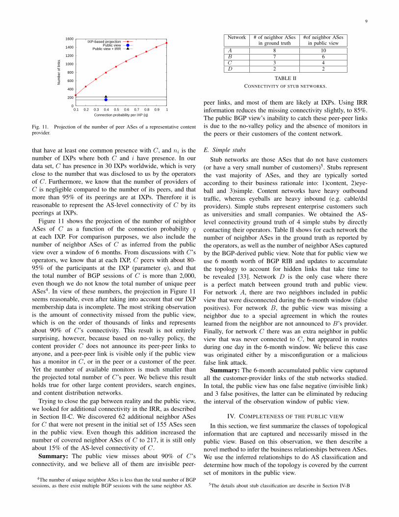
that have at least one common presence with C, and ni is thenumber of IXPs where both C and i have presence. In ourdata set, C has presence in 30 IXPs worldwide, which is veryclose to the number that was disclosed to us by the operatorsof C. Furthermore, we know that the number of providers ofC is negligible compared to the number of its peers, and thatmore than 95% of its peerings are at IXPs. Therefore it isreasonable to represent the AS-level connectivity of C by itspeerings at IXPs.

Figure 11 shows the projection of the number of neighborASes of C as a function of the connection probability qat each IXP. For comparison purposes, we also include thenumber of neighbor ASes of C as inferred from the publicview over a window of 6 months. From discussions with C’soperators, we know that at each IXP, C peers with about 80-95% of the participants at the IXP (parameter q), and thatthe total number of BGP sessions of C is more than 2,000,even though we do not know the total number of unique peerASes4. In view of these numbers, the projection in Figure 11seems reasonable, even after taking into account that our IXPmembership data is incomplete. The most striking observationis the amount of connectivity missed from the public view,which is on the order of thousands of links and representsabout 90% of C’s connectivity. This result is not entirelysurprising, however, because based on no-valley policy, thecontent provider C does not announce its peer-peer links toanyone, and a peer-peer link is visible only if the public viewhas a monitor in C, or in the peer or a customer of the peer.Yet the number of available monitors is much smaller thanthe projected total number of C’s peer. We believe this resultholds true for other large content providers, search engines,and content distribution networks.

Trying to close the gap between reality and the public view,we looked for additional connectivity in the IRR, as describedin Section II-C. We discovered 62 additional neighbor ASesfor C that were not present in the initial set of 155 ASes seenin the public view. Even though this addition increased thenumber of covered neighbor ASes of C to 217, it is still onlyabout 15% of the AS-level connectivity of C.

Summary: The public view misses about 90% of C’sconnectivity, and we believe all of them are invisible peer-

4The number of unique neighbor ASes is less than the total number of BGPsessions, as there exist multiple BGP sessions with the same neighbor AS.

Network # of neighbor ASes #of neighbor ASesin ground truth in public view

A 8 10B 7 6C 3 4D 2 2

TABLE IICONNECTIVITY OF STUB NETWORKS.

peer links, and most of them are likely at IXPs. Using IRRinformation reduces the missing connectivity slightly, to 85%.The public BGP view’s inability to catch these peer-peer linksis due to the no-valley policy and the absence of monitors inthe peers or their customers of the content network.

E. Simple stubs

Stub networks are those ASes that do not have customers(or have a very small number of customers)5. Stubs representthe vast majority of ASes, and they are typically sortedaccording to their business rationale into: 1)content, 2)eye-ball and 3)simple. Content networks have heavy outboundtraffic, whereas eyeballs are heavy inbound (e.g. cable/dslproviders). Simple stubs represent enterprise customers suchas universities and small companies. We obtained the AS-level connectivity ground truth of 4 simple stubs by directlycontacting their operators. Table II shows for each network thenumber of neighbor ASes in the ground truth as reported bythe operators, as well as the number of neighbor ASes capturedby the BGP-derived public view. Note that for public view weuse 6 month worth of BGP RIB and updates to accumulatethe topology to account for hidden links that take time tobe revealed [33]. Network D is the only case where thereis a perfect match between ground truth and public view.For network A, there are two neighbors included in publicview that were disconnected during the 6-month window (falsepositives). For network B, the public view was missing aneighbor due to a special agreement in which the routeslearned from the neighbor are not announced to B’s provider.Finally, for network C there was an extra neighbor in publicview that was never connected to C, but appeared in routesduring one day in the 6-month window. We believe this casewas originated either by a misconfiguration or a maliciousfalse link attack.

Summary: The 6-month accumulated public view capturedall the customer-provider links of the stub networks studied.In total, the public view has one false negative (invisible link)and 3 false positives, the latter can be eliminated by reducingthe interval of the observation window of public view.

IV. COMPLETENESS OF THE PUBLIC VIEW

In this section, we first summarize the classes of topologicalinformation that are captured and necessarily missed in thepublic view. Based on this observation, we then describe anovel method to infer the business relationships between ASes.We use the inferred relationships to do AS classification anddetermine how much of the topology is covered by the currentset of monitors in the public view.

5The details about stub classification are describe in Section IV-B

10

A. ”Public view” vs. ground truth

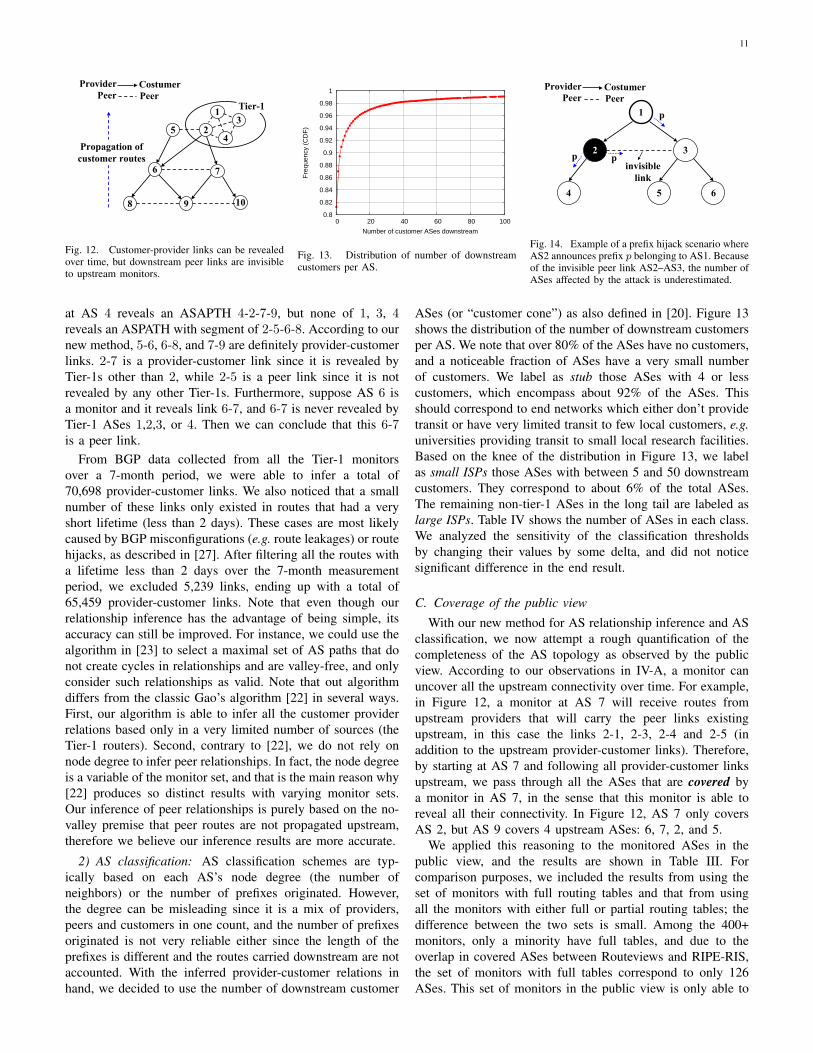
We use Figure 12 as an illustration to summarize the degreeof completeness of the observed topology as seen by the publicview. Our observations presented here are the natural resultsof the no-valley-and-prefer-customer policy, and some of themhave been speculated briefly in previous work. In this paper wequantify and verify the degree of completeness by comparingthe ground truth with the observed topology. Though the fewclasses of networks we have examined are not necessarilyexhaustive, we believe the observations drawn from these casestudies provide insights that are valid for the Internet as awhole.

First, if a monitor resides in an AS A, the public viewshould be able to capture all of A’s direct links, includingboth customer-provider and peer links. However, not all thelinks of the AS may show up in a snapshot observation. Ittakes time, which may be as long as a few years, to have allhidden customer-provider links exposed by routing dynamics.Second, a monitor in a provider network should be able tocapture all the provider-customer links between itself and allof its downstream customers, and a monitor in a customernetwork should be able to capture all the customer-providerlinks between itself and its upstream providers. For example,in Figure 12, a monitor in AS2 can capture not only its directprovider-customer links (2-6 and 2-7), but also the provider-customer links between its downstream customers (6-8, 6-9,7-9, and 7-10). AS5, as a peer of AS2, is also able to captureall the provider-customer links downstream of AS2 since AS2will announce its customer routes to its peers. Again, it cantake quite a long time to reveal all the hidden links. Third,a monitor cannot observe a peer link of its customer, or peerlinks of its neighbors at the same tier 6. For example, a monitorat AS5 will not be able to capture the peer link 6-7 or 1-2,because a peer route is not announced to providers or otherpeers according to the no-valley policy. Fourth, to capture apeer link requires a monitor in one of the peer ASes or in adownstream customer of the two ASes incident to the link. Forexample, a monitor at AS9 can observe the peer links 6-7 and5-2, but not the peer link 1-3 since AS9 is not a downstreamcustomer of either AS1 or AS3.

The current public view has monitors in all the Tier-1 ASesexcept one, and that particular Tier-1 AS has a direct customerAS that hosts a monitor. Applying the above observations, wecan summarize and generalize the completeness of the AS-level topology captured by the public view as follows.• Coverage of Tier-1 links: The public view contains all

the links of all the Tier-1 ASes.• Coverage of customer-provider links: There is no in-

visible customer-provider link. Thus over time the publicview should be able to reveal all the customer-providerlinks in the Internet topology, i.e. , the number of hiddencustomer-provider links should gradually approach zerowith the increase of the observation period length. Thisis supported by our empirical findings: in all our casestudies we found all the customer-provider links fromBGP data collected over a few years.

6We assume that the provider-customer links do not form a circle.

• Coverage of peer links: The public view misses alarge number of peer links, especially peer links betweenlower tier ASes in the Internet routing hierarchy. Thepublic view will not capture a peer link A–B unlessthere is a monitor installed in either A or B, or in adownstream customer of A or B. Presently, the publicmonitors are in about 400+ ASes out of a total over27,000 existing ASes, this ratio gives a rough perspectiveon the percentage of peer links missing from the publicview. Peer links between stub networks (i.e. , links 8-9 and 9-10 in Figure 12) are among the most difficultones to capture. Unfortunately, with the recent growthof content networks, it is precisely these links that arerapidly increasing in numbers.

B. Network Classification

The observations from the last section led us to a novel andsimple method for inferring the business relationships betweenASes, that allow us also to classify ASes in different types.

1) Inferring AS Relationships: The last section concludedthat, assuming routes follow a no-valley policy, monitors at thetop of the routing hierarchy (i.e. those in Tier-1 ASes) are ableto reveal all the downstream provider-customer connectivityover time. This is an important observation since, by definition,each non-Tier-1 AS is a customer of at least one Tier-1 AS,then essentially all the provider-customer links in the topologycan be observed by the Tier-1 monitors over time. This is thebasic idea of our AS relationship inference algorithm.

We start with the assumption that the set of Tier-1 ASesis already known7. By definition of Tier-1 ASes, all linksbetween Tier-1s are peer links, and a Tier-1 AS is not acustomer of any other ASes. Suppose a monitor at Tier-1AS m reveals an ASPATH m-a1-a2-...-an. The link m-a1

can be either a provider-customer link, or a peer link (this isbecause in certain cases a Tier-1 may have a specially arrangedpeer relationship with a lower-tiered AS). However, accordingto the no-valley policy, a1-a2, a2-a3, ... , an−1-an must beprovider-customer links, because a peer or provider routeshould not be propagated upstream from a1 to m. Thereforethe segment a2, ..., an must correspond to a customer routereceived by a1. To infer the relationship of m-a1, we note thataccording to no-valley policy, if m-a1 is a provider-customerlink, this link should appear in the routes propagated fromm to other Tier-1 ASes, whose monitors will reveal this link.On the other hand, if m-a1 is a peer link, it should neverappear in the routes received by the monitors in other Tier-1 ASes. Given we have monitors in all Tier-1 ASes or theircustomer ASes, we can accurately infer the relationship m-a1 by examining whether it is revealed by other Tier-1 ASes.Using this method, we can first find and label all the provider-customer links, and then label all the other links revealed bythe monitors as peer links.

Our algorithm is illustrated in Figure 12, where 1, 2, 3, and4 are known to be Tier-1s. Suppose AS 2 monitor reveals anASPATH 2-5-6-8 and another ASPATH 2-7-9; while monitors

7The list of Tier-1 ASes can be obtained from website such as http://en.wikipedia.org/wiki/Tier 1 carrier

11

2

Provider CostumerPeer Peer

13

45

8

Tier-1

76

9 10

Propagation ofcustomer routes

Fig. 12. Customer-provider links can be revealedover time, but downstream peer links are invisibleto upstream monitors.

0.8

0.82

0.84

0.86

0.88

0.9

0.92

0.94

0.96

0.98

1

0 20 40 60 80 100

Fre

quen

cy (

CD

F)

Number of customer ASes downstream

Fig. 13. Distribution of number of downstreamcustomers per AS.

1

2 3

Provider CostumerPeer Peer

65

p

p

4

pinvisiblelink

Fig. 14. Example of a prefix hijack scenario whereAS2 announces prefix p belonging to AS1. Becauseof the invisible peer link AS2–AS3, the number ofASes affected by the attack is underestimated.

at AS 4 reveals an ASAPTH 4-2-7-9, but none of 1, 3, 4reveals an ASPATH with segment of 2-5-6-8. According to ournew method, 5-6, 6-8, and 7-9 are definitely provider-customerlinks. 2-7 is a provider-customer link since it is revealed byTier-1s other than 2, while 2-5 is a peer link since it is notrevealed by any other Tier-1s. Furthermore, suppose AS 6 isa monitor and it reveals link 6-7, and 6-7 is never revealed byTier-1 ASes 1,2,3, or 4. Then we can conclude that this 6-7is a peer link.

From BGP data collected from all the Tier-1 monitorsover a 7-month period, we were able to infer a total of70,698 provider-customer links. We also noticed that a smallnumber of these links only existed in routes that had a veryshort lifetime (less than 2 days). These cases are most likelycaused by BGP misconfigurations (e.g. route leakages) or routehijacks, as described in [27]. After filtering all the routes witha lifetime less than 2 days over the 7-month measurementperiod, we excluded 5,239 links, ending up with a total of65,459 provider-customer links. Note that even though ourrelationship inference has the advantage of being simple, itsaccuracy can still be improved. For instance, we could use thealgorithm in [23] to select a maximal set of AS paths that donot create cycles in relationships and are valley-free, and onlyconsider such relationships as valid. Note that out algorithmdiffers from the classic Gao’s algorithm [22] in several ways.First, our algorithm is able to infer all the customer providerrelations based only in a very limited number of sources (theTier-1 routers). Second, contrary to [22], we do not rely onnode degree to infer peer relationships. In fact, the node degreeis a variable of the monitor set, and that is the main reason why[22] produces so distinct results with varying monitor sets.Our inference of peer relationships is purely based on the no-valley premise that peer routes are not propagated upstream,therefore we believe our inference results are more accurate.

2) AS classification: AS classification schemes are typ-ically based on each AS’s node degree (the number ofneighbors) or the number of prefixes originated. However,the degree can be misleading since it is a mix of providers,peers and customers in one count, and the number of prefixesoriginated is not very reliable either since the length of theprefixes is different and the routes carried downstream are notaccounted. With the inferred provider-customer relations inhand, we decided to use the number of downstream customer

ASes (or “customer cone”) as also defined in [20]. Figure 13shows the distribution of the number of downstream customersper AS. We note that over 80% of the ASes have no customers,and a noticeable fraction of ASes have a very small numberof customers. We label as stub those ASes with 4 or lesscustomers, which encompass about 92% of the ASes. Thisshould correspond to end networks which either don’t providetransit or have very limited transit to few local customers, e.g.universities providing transit to small local research facilities.Based on the knee of the distribution in Figure 13, we labelas small ISPs those ASes with between 5 and 50 downstreamcustomers. They correspond to about 6% of the total ASes.The remaining non-tier-1 ASes in the long tail are labeled aslarge ISPs. Table IV shows the number of ASes in each class.We analyzed the sensitivity of the classification thresholdsby changing their values by some delta, and did not noticesignificant difference in the end result.

C. Coverage of the public view

With our new method for AS relationship inference and ASclassification, we now attempt a rough quantification of thecompleteness of the AS topology as observed by the publicview. According to our observations in IV-A, a monitor canuncover all the upstream connectivity over time. For example,in Figure 12, a monitor at AS 7 will receive routes fromupstream providers that will carry the peer links existingupstream, in this case the links 2-1, 2-3, 2-4 and 2-5 (inaddition to the upstream provider-customer links). Therefore,by starting at AS 7 and following all provider-customer linksupstream, we pass through all the ASes that are covered bya monitor in AS 7, in the sense that this monitor is able toreveal all their connectivity. In Figure 12, AS 7 only coversAS 2, but AS 9 covers 4 upstream ASes: 6, 7, 2, and 5.

We applied this reasoning to the monitored ASes in thepublic view, and the results are shown in Table III. Forcomparison purposes, we included the results from using theset of monitors with full routing tables and that from usingall the monitors with either full or partial routing tables; thedifference between the two sets is small. Among the 400+monitors, only a minority have full tables, and due to theoverlap in covered ASes between Routeviews and RIPE-RIS,the set of monitors with full tables correspond to only 126ASes. This set of monitors in the public view is only able to

12

Parameter Full tables Full+partial tablesNo. monitored 121 411

ASesCovered ASes 1,101 / 28,486 ' 4% 1,552 / 28,486 ' 5 %

TABLE IIICOVERAGE OF BGP MONITORS.

Type ASes Monitored Covered ASesASes aggregated by covering type

Tier-1 9 8 9 (100%) 8Large ISP 436 45 337 (77.3%) 954Small ISP 1,829 36 629 (34.4%) 269

Stubs 26,209 37 126 (0.5%) 160

TABLE IVCOVERAGE OF BGP MONITORS FOR DIFFERENT NETWORK TYPES.

cover 4% of the total number of ASes in Internet. This resultindicates that the AS topologies derived from the public view,which have been widely used by the research community, maymiss most of the peer connectivity within the remaining 96%of the ASes (or 57% of the transits).

Finally, we look at the covered ASes in terms of theirclasses, which is shown in Table IV. The column “CoveredASes-aggregated” refers to the fraction of covered ASes ineach AS class, whereas the column “Covered ASes-by cover-ing type” refers to the total number of ASes covered by themonitors in each class. For instance, 77.3% of the large ISPsare covered by monitors, and monitors in large ISPs covera total of 954 total ASes. The numbers in the table indicatethat Tier-1s are fully covered, large ISPs are mostly covered,small ISPs remain largely uncovered (just 34.4%), and stubsare almost completely uncovered (99.5%). These results aredue to the fact that most of the monitors reside in the coreof the network. In order to cover a stub, we would need toplace a monitor in that stub, which is infeasible due to thevery large number of stubs in Internet.

V. DISCUSSION

The defects in the inferred AS topologies, as revealed byour case studies, may have different impacts on the differentresearch projects and studies that use an inferred AS topology.In the following, we use a few specific examples to illustratesome of the problems that can arise.

Stub AS growth rates and network diameter: Given thatthe public view captures almost all the AS nodes and customer-provider links, it provides an adequate data source for studieson AS-topology metrics including network diameter; growthrates and trends for the number of stub ASes; and quantifyingcustomer multihoming (where multihoming here does notaccount peer links).

Other graph-theoretic metrics: Given that the public viewis largely inadequate in covering peer links, and given thatthese peer links typically allow for shortcuts in the data plane,relying on the public view can clearly cause major distortionswhen studying generic graph properties such as node degrees,path lengths, node clustering, etc.

Impact of prefix hijacking: Prefix hijacking is a serioussecurity threat facing Internet and happens when an ASannounces prefixes that belong to other ASes. Recent work

on this topic [25], [45], [15], [42] evaluates the proposedsolutions by using the inferred AS topologies from the publicview. Depending on the exact hijack scenario, an incompletetopology can lead to either an underestimate or overestimate ofthe hijack impact. Figure 14 shows an example of a hijack sim-ulation scenario, where AS2 announces prefix p that belongsto AS1. Because of the invisible peer link 1–2, the numberof impacted ASes is underestimated, i.e. ASes 3,5 and 6 arebelieved to pick the route originated by AS1, whereas in realitythey would pick the more preferred peer route coming from thehijacker AS2. At the same time, an incomplete topology couldalso lead simulations to overestimate the impact of a hijack.For example, the content network C considered in Section IIIhas a large number of direct peers who are unlikely to beimpacted by a hijack from a remote AS, so missing 90% ofC’s peer links in the topology would significantly overestimatethe impact of such a hijack. On the other hand, if C is ahijacker, then the incomplete topology would result in a vastunderestimation of the impact.

Relationship inference/path inference: Several studieshave addressed the problem of inferring the relationship be-tween ASes based on observed routing paths [22], [39], [28].There can be cases where customer-provider links are wronglyinferred as peer links based on the observed set of paths,creating a no-valley violation. Knowledge of the invisible peerlinks in paths could avoid some of these errors. The pathinference heuristics [28], [30], [31] are also impacted by theincompleteness problem, mainly because they a priori excludeall paths that traverse invisible peer links.

Routing resiliency to failures: Studies that address robust-ness properties of the Internet under different failure scenarios(e.g., see [21], [42]) also heavily depend on having a completeand accurate AS-level topology, on top of which failures aresimulated. One can easily envision scenarios where two partsof the network are thought to become disconnected after afailure, while in reality there are invisible peer links connectingthem. Given that currently inferred AS maps tend to missa substantial number of peer links, robustness-related claimsbased these inferred maps need to be viewed with a grain ofsalt.

Evaluation of new inter-domain protocols: The evaluationof new inter-domain routing protocols also heavily relies onthe accuracy of the AS-level topology over which a newprotocol is supposed to run. For instance, [40] proposes a newprotocol where a path-vector protocol is used among Tier-1 ASes, and all the ASes under each Tier-1 run link-staterouting. The design is based on an assumption that customertrees of Tier-1 ASes are largely disjoint, and violations of thisassumption are handled as rare exceptions. However, in viewof our findings, there are a substantial number of invisiblepeer links interconnecting ASes at lower tier and aroundthe edge of Internet, therefore connectivity between differentcustomer trees becomes the rule rather than the exception. Wewould imagine the performance of the proposed protocol undercomplete and incomplete topologies to be different, possiblyquite significantly.

13

VI. RELATED WORK

Three main types of data sets have been available for AS-level topology inference: (1) BGP tables and updates, (2)traceroute measurements, and (3) Internet Routing Registry(IRR) information. BGP tables and updates have been col-lected by the University of Oregon RouteViews project [12]and by RIPE-RIS in Europe [11]. Traceroute-based datasetshave been gathered by CAIDA as part of the Skitter project[13], by an EU-project called Dimes [37], and more recentlyby the iPlane project [26]. Other efforts have extended theabove measurements by including data from the InternetRouting Registry [17], [38], [43]. However, studies that havecritically relied on these topology measurements have rarelyexamined the data quality in detail, thus the (in)sensitivity ofthe results and claims to the known or suspected deficienciesin the measurements has largely gone unnoticed.

Chang et al. [17], [19], [16] were among the first to studythe completeness of commonly used BGP-derived topologymaps; later studies [44], [34], [43], using different datasources, yielded similar results confirming that 40% or moreAS links may exist in the actual Internet but are missed bythe BGP-derived AS maps. He et al. [43] report an additional300% of peer links in IRR compared to those extracted fromBGP data, however this percentage is likely inflated sincethey only took RIB snapshots from 35 of the ∼700 routersproviding BGP feeds to RouteViews and RIPE-RIS. All theseefforts have in common that they try to incrementally closethe completeness gap, without first quantifying the degree of(in)completeness of currently inferred AS maps. Our paperrelies on the ground truth of AS-level connectivity of differenttypes of ASes to shed light on what and how much is missingfrom the commonly-used AS maps and why. Dimitropouloset al. [20] use AS adjacencies as reported by several ISPs tovalidate an AS relationship inference heuristic. They foundthat most links reported by ISPs that are not in the publicview are peer links. In contrast to their work, most of ourfindings are inferred from iBGP tables, router configs, andsyslog records collected over time from thousands of routers.Our approach yields an accurate picture of the ground truth asfar as BGP adjacencies are concerned and allows us to verifyprecisely for each AS link x, why x was missing from publicview. Lastly, in view of the recent work [36] that concludesthat an estimated 700 route monitors would suffice to see99.9% of all AS-links, our approach shows that such an overallestimate comes with an important qualifier: what is importantis not the total number of monitors, but their locations withinthe AS hierarchy. In fact, our findings suggest a simple strategyfor placing monitors to uncover the bulk of missing links, butunfortunately researchers have in general little input when itcomes to the actual placement of new monitors.

VII. CONCLUSION

In this paper, we demonstrated the infeasibility to obtain acomplete AS-level topology through the current data collectionefforts, a direction that has been pursued in the past. We alsoattacked the problem from a new and different angle: obtaining

the ground truth of a sample set of ASes’ connectivity struc-tures and comparing them with the AS connectivity inferredfrom publicly available data sets. This approach enabled us todeepen our understanding of which parts of the actual AStopology are captured in the public view and which partsremain invisible and are missing from the public view*.

A critical aspect of our search for the elusive ground truth ofAS-level Internet connectivity and of the proposed pragmaticapproach to constructing realistic and viable AS maps is thatthey both treat ASes as objects with a rich, important, anddiverse internal structure, and not as generic and property-lessnodes. Exploiting this structure is at the heart of our work. Thenature of this AS-internal structure permeates our definitionof “ground truth” of AS-level connectivity, our analysis of theavailable data sets, our understanding of the reasons behindand importance of the deficiencies of commonly-used AS-level Internet topologies, and our proposed efforts to constructrealistic and viable maps of the Internet’s AS-level ecosystem.Faithfully accounting for this internal structure can also beexpected to favor the constructions of AS maps that withstandscrutiny by domain experts. Such constructions also stand abetter chance to represent fully functional and economicallyviable AS-level topologies than models where the intercon-nections between different ASes are solely determined byindependent coin tosses.

ACKNOWLEDGEMENTS

We would like to thank Tom Scholl, Bill Woodcock, RenProvo, Jay Borkenhagen, Jennifer Yates, Seungjoon Lee, AlexGerber and Aman Shaikh for many helpful discussions. Wewould also like to thank several network operators who helpedus gain insight into the AS-level Internet connectivity.

REFERENCES

[1] AOL peering requirements. http://www.atdn.net/settlement free int.shtml.[2] AT&T peering requirements. http://www.corp.att.com/peering/.[3] CERNET BGP feeds. http://bgpview.6test.edu.cn/bgp-view/.[4] European Internet exchange association. http://www.euro-ix.net.[5] Geant2 looking glass. http://stats.geant2.net/lg/.[6] Good practices in Internet exchange points.

http://www.pch.net/resources/papers/ix-documentation-bcp/ix-documentation-bcp-v14en.pdf.

[7] Internet Routing Registry. http://www.irr.net/.[8] Packet clearing house IXP directory. http://www.pch.net/ixpdir/Main.pl.[9] PeeringDB website. http://www.peeringdb.com/.

[10] Personal Communication with Bill Woodcock@PCH.[11] RIPE routing information service project. http://www.ripe.net/.[12] RouteViews routing table archive. http://www.routeviews.org/.[13] Skitter AS adjacency list. http://www.caida.org/tools/measurement/skitter

/as adjacencies.xml.[14] The Abilene Observatory Data Collections.

http://abilene.internet2.edu/observatory/data-collections.html.[15] H. Ballani, P. Francis, and X. Zhang. A study of prefix hijacking and

interception in the Internet. In Proc. of ACM SIGCOMM, 2007.[16] H. Chang. An Economic-Based Empirical Approach to Modeling

the Internet Inter-Domain Topology and Traffic Matrix. PhD thesis,University of Michigan, 2006.

[17] H. Chang, R. Govindan, S. Jamin, S. J. Shenker, and W. Willinger.Towards capturing representative AS-level Internet topologies. ElsevierComputer Networks Journal, 44(6):737–755, 2004.

[18] H. Chang, S. Jamin, and W. Willinger. Inferring AS-level Internettopology from router-level path traces. In SPIE ITCom, 2001.

[19] H. Chang and W. Willinger. Difficulties measuring the Internet’s AS-level ecosystem. In Annual Conference on Information Sciences andSystems (CISS’06), pages 1479–1483, 2006.

14

[20] X. Dimitropoulos, D. Krioukov, M. Fomenkov, B. Huffaker, Y. Hyun,kc claffy, and G. Riley. As relationships: inference and validation. ACMSIGCOMM Comput. Commun. Rev., 2007.

[21] D. Dolev, S. Jamin, O. Mokryn, and Y. Shavitt. Internet resiliencyto attacks and failures under bgp policy routing. Computer Networks,50(16):3183–3196, 2006.

[22] L. Gao. On inferring autonomous system relationships in the Internet.IEEE/ACM Transactions on Networking, 9(6):733–745, 2001.

[23] B. Hummel and S. Kosub. Acyclic type-of-relationship problems on theinternet: an experimental analysis. In ACM IMC, 2007.

[24] Y. Hyun, A. Broido, and kc claffy. On third-party addresses in traceroutepaths. In Proc. of Passive and Active Measurement Workshop (PAM),2003.

[25] M. Lad, R. Oliveira, B. Zhang, and L. Zhang. Understanding theresiliency of Internet topology against false origin attacks. In Proc.of IEEE DSN, 2007.

[26] H. Madhyastha, T. Isdal, M. Piatek, C. Dixon, T. Anderson, A. Kr-ishnamurthy, and A. Venkataramani. iPlane: an information plane fordistributed services. In Proc. of OSDI, 2006.

[27] R. Mahajan, D. Wetherall, and T. Anderson. Understanding BGPMisconfiguration. In In Proc. of ACM SIGCOMM, 2002.

[28] Z. M. Mao, L. Qiu, J. Wang, and Y. Zhang. On AS-level path inference.In Proc. SIGMETRICS, 2005.

[29] Z. M. Mao, J. Rexford, J. Wang, and R. H. Katz. Towards an accurateAS-level traceroute tool. In Proc. of ACM SIGCOMM, 2003.

[30] W. Muhlbauer, A. Feldmann, O. Maennel, M. Roughan, and S. Uhlig.Building an AS-topology model that captures route diversity. In Proc.of ACM SIGCOMM, 2006.

[31] W. Muhlbauer, S. Uhlig, B. Fu, M. Meulle, and O. Maennel. In searchfor an appropriate granularity to model routing policies. In Proc. ofACM SIGCOMM, 2007.

[32] R. Oliveira, B. Zhang, D. Pei, R. Izhak-Ratzin, and L. Zhang. Quanti-fying Path Exploration in the Internet. In ACM Internet MeasurementConference (IMC), October 2006.

[33] R. Oliveira, B. Zhang, and L. Zhang. Observing the evolution of InternetAS topology. In ACM SIGCOMM, 2007.

[34] D. Raz and R. Cohen. The Internet dark matter: on the missing linksin the AS connectivity map. In Proc. of IEEE INFOCOM, 2006.

[35] Y. Rekhter, T. Li, and S. Hares. Border Gateway Protocol 4. RFC 4271,Internet Engineering Task Force, January 2006.

[36] M. Roughan, S. J. Tuke, and O. Maennel. Bigfoot, sasquatch, the yetiand other missing links: what we don’t know about the as graph. InACM IMC, 2008.

[37] Y. Shavitt and E. Shir. DIMES: Let the Internet measure itself. ACMSIGCOMM Computer Comm. Review (CCR), 2005.

[38] G. Siganos and M. Faloutsos. Analyzing BGP policies: Methodologyand tool. In Proc. of IEEE INFOCOM, 2004.

[39] L. Subramanian, S. Agarwal, J. Rexford, and R. Katz. Characterizing theinternet hierarchy from multiple vantage points. In INFOCOM, 2002.

[40] L. Subramanian, M. Caesar, C. T. Ee, M. Handley, M. Mao, S. Shenker,and I. Stoica. HLP: a next generation inter-domain routing protocol. InProc. ACM SIGCOMM, 2005.

[41] L. Wang, M. Saranu, J. M. Gottlieb, and D. Pei. Understanding BGPsession failures in a large ISP. In Proc. of IEEE INFOCOM, 2007.

[42] J. Wu, Y. Zhang, Z. Mao, and K. Shin. Internet routing resilience tofailures: analysis and implications. In Proc. of ACM CoNext, 2007.

[43] Y. He, G. Siganos, M. Faloutsos, S. V. Krishnamurthy. A systematicframework for unearthing the missing links: measurements and impact.In Proc. of NSDI, 2007.

[44] B. Zhang, R. Liu, D. Massey, and L. Zhang. Collecting the InternetAS-level topology. ACM SIGCOMM Computer Comm. Review (CCR),35(1):53–61, 2005.

[45] C. Zheng, L. Ji, D. Pei, J. Wang, and P. Francis. A light-weightdistributed scheme for detecting IP prefix hijacks in real-time. In Proc.of ACM SIGCOMM, 2007.

Ricardo Oliveira received the B.S. in ElectricalEngineering from the Engineering Faculty of PortoUniversity (FEUP), Portugal in 2001 and the M.S.degree in Computer Science from University of Cal-ifornia, Los Angeles in 2005. He has been pursuingthe Ph.D. in Computer Science at University ofCalifornia, Los Angeles, since 2005. He is a studentmember of the ACM and the IEEE.

Dan Pei is a researcher at AT&T Research. Hereceived his Ph.D. degree from UCLA in 2005, andhis B.S. and M.S. degrees from Tsinghua Universityin 1997 and 2000. His current research interests arenetwork measurement and security.

Walter Willinger received the diploma (Dipl.Math.) from the ETH Zurich, Switzerland, and theM.S. and Ph.D. degrees from Cornell University,Ithaca, NY. He is currently a member of the Informa-tion and Software Systems Research at AT&T Labs- Research, Florham Park, NJ. He was a Memberof the Technical Staff at Bellcore Applied Researchfrom 1986 to 1996. He was a co-recipient of the1996 IEEE W.R. G. Baker Prize Award and the 1994IEEE W.R. Bennett Prize Paper Award. He is anACM Fellow, an IEEE Fellow, and an AT&T Fellow.

Beichuan Zhang is an Assistant Professor in theDepartment of Computer Science at the Universityof Arizona. His research interests include Internetrouting and topology, multicast, network measure-ment, and security. He received Ph.D. in ComputerScience from the University of California, Los An-geles (2003) and B.S. from Peking University, China(1995).

Lixia Zhang is a professor in the Computer ScienceDepartment of UCLA. She received her Ph.D incomputer science from the Massachusetts Institute ofTechnology and was a member of the research staffat Xerox Palo Alto Research Center before joiningUCLA in 1996. Zhang is a member of the InternetArchitecture Board (IAB). She is an ACM Fellowand IEEE Fellow.