THE INCREMENTAL INFORMATION CONTENT OF ANALYSTS’ RESEARCH

REPORTS AND FIRMS’ ANNUAL REPORTS:

EVIDENCE FROM TEXTUAL ANALYSIS

JUNE WOO PARK

A DISSERTATION SUBMITTED TO

THE FACULTY OF GRADUATE STUDIES

IN PARTIAL FULFILLMENT OF THE REQUIREMENTS

FOR THE DEGREE OF

DOCTOR OF PHILOSOPHY

GRADUATE PROGRAM IN ACCOUNTING

YORK UNIVERSITY

TORONTO, ONTARIO

JUNE 2019

© June Woo Park, 2019

ii

Abstract

This dissertation consists of three essays, investigating the properties of analysts’

research reports and firms’ annual reports, and their impact on capital markets using textual

analysis methods.

The first essay studies the validity of analyst report length, measured by page count, as a

proxy for analysts’ research effort. Specifically, I find that longer reports are more positively

associated with recommendation upgrades than downgrades, and with forecast accuracy. I

further document an asymmetric market reaction to longer upgrades as compared to the same

length downgrades. Cross-sectional tests find that this asymmetric report length effect is greater

for longer upgrade reports with more cash flow discussion, by less experienced, busier, or male

analysts, for high opaque firms, or during a financial crisis. The findings support my hypothesis

that by providing more and accurate information, analysts exert credibility-enhancing efforts on

their upgrades, as these are perceived by investors to be more optimistic and less credible than

downgrades. The study is the first comprehensive investigation of analysts’ research effort for

U.S. firms using the number of pages in their reports and suggests differing interpretations of

analyst vs. annual report length as a proxy. In other words, management tends to write a longer

annual report to hide bad news, whereas analysts tend to write a longer analyst report to provide,

and not hide, more information to increase report credibility.

In a second textual analysis essay, I examine the determinants of environmental

disclosures (ED) in U.S. 10-Ks (i.e. annual reports) and its impact on future stock price crash

risk. I provide crucial evidence that ED is related to bad news (i.e. news that tends to be

obfuscated by managers) by showing the autocorrelation of its change over time and its negative

association with short-term market reaction. In the long run, however, an increase in ED shows a

iii

lower likelihood of significant stock price drops. Change and instrument variable analyses

mitigate endogeneity and identify a potential causality of ED on the future crash risk. The results

are consistent with the notion that firms benefit from non-financial information disclosure.

A third textual analysis essay compares the value of private versus public information

sources in U.S. analysts’ earnings forecasts. Using a pattern search algorithm (i.e., regular

expression) on the headlines of earnings forecasts, I find that additional private sources of

information are associated with (or may cause) less forecast error, triggering a greater market

reaction. Moreover, I document that the combination of management and non-management

private information sources minimizes forecast error and maximizes market reaction. Thus, such

a combination tends to produce the most accurate forecasts and, as a result, the strongest market

reaction. Finally, I show that more accurate and informative forecasts are made by analysts who

make greater efforts to access private information sources, even when they do not have other

information advantages (e.g. brokerage firm reputation). Thus, I provide new insight into the

determinants of forecast properties.

Overall, the above-noted studies show that the length and the information sources of

analysts’ research reports significantly influence investors’ decision making. The essays also

suggest that environmental disclosure in firms’ annual reports contributes to a decrease in future

stock price crash risk.

iv

Acknowledgments

First of all, I would like to thank my dissertation committee: Dr. Albert Tsang (chair), Dr.

Kiridaran (Giri) Kanagaretnam, Dr. Kee-Hong Bae, Dr. Gary Spraakman, and Dr. Tracy (Kun)

Wang for their advice and constructive feedback on my dissertation.

Especially, I would like to acknowledge my deepest gratitude to Dr. Albert Tsang, my

supervisor and thesis advisor, for his invaluable detailed guidance, thoughtful correction, his

confidence in my ability to carry the work out, and his great encouragement at each stage of my

doctoral studies. This thesis would not have been possible without his wisdom, feedback, and

support. Thank you for also being my friend and family.

I am incredibly fortunate to have Dr. Hongping Tan, my former advisor. His constant

support and guidance have made my PhD study a fruitful journey. I will be forever indebted to

you.

I am also highly indebted to Dr. Kee-Hong Bae, my mentor. I appreciate his insightful

comments and continuing encouragement throughout the process. He is very kind and

supportive. This thesis has been considerably improved as a result of his insightful suggestions.

I greatly thank Dr. Kiridaran (Giri) Kanagaretnam for caring me like a big brother. Your

guidance and philosophy have shaped my thinking not only in research but also in life. There are

no words that can truly express my gratitude to you for everything.

This journey would not have been possible without the great support that I have received

from my family over the years.

I have to say thank you to my loving parents, Hyun Soo Park and Song Gang Kim. I

would like to express my sincere gratitude for raising me to be who I am today with your

v

unconditional love. I thank you for supporting me in everything I wanted to do in life. I could not

have hoped for better parents. I earnestly pray for my father’s fast and easy recovery.

vi

Table of Contents

Abstract..................................................................................................................... ......................ii

Acknowledgments..........................................................................................................................iv

Table of Contents............................................................................................................................vi

Essay 1 Abstract.……………………..............................................................................................1

Chapter 1 Introduction................................................................................................................2

Chapter 2 Literature review on annual vs. analyst report length and Hypotheses

development.............................................................................................................7

2.1 Annual report (Form 10-K) length: proxy for complexity………………………..7

2.2 Analyst report length: proxy for analyst research effort………………………….8

2.3 Credibility-enhancing hypothesis……………………………………………….11

Chapter 3 Research methodology and sample selection……………………………………...14

3.1 Measurement of report length…………………………………………………...14

3.2 Measurement of earnings forecast error and informativeness…………………..15

3.3 Regression specification………………………………………………………...16

3.4. Sample selection………………………………………………………………..18

Chapter 4 Empirical results…………………………………………………………………...19

4.1 Descriptive statistics…………………………………………………………….19

4.2 Univariate test…………………………………………………………………...21

4.3 Main regression analyses………………………………………………………..21

4.3.1 Determinants of report length……………………………………………...22

4.3.2 Report length and earnings forecast accuracy……………………………..23

4.3.3 Report length and stock recommendation informativeness………………..24

vii

Chapter 5 Robustness checks…………………………………………………………………26

5.1 Recommendation levels: buy and sell…………………………………………...26

5.2 Within-bank analysis……………………………………………………………27

5.3 Extended market reaction model………………………………………………..27

Chapter 6 Cross-sectional test on market reaction to longer revisions……………………….28

6.1 Detailed information traits………………………………………………………28

6.2 Analyst characteristics…………………………………………………………..29

6.3 Information environment effect…………………………………………………30

Chapter 7 Report length and forecast frequency……………………………………………...32

Chapter 8 Conclusion…………………………………………………………………………33

References………………………………………………………………………………….....36

Essay 2 Abstract….........................................................................................................................58

Chapter 1 Introduction..............................................................................................................59

Chapter 2 Literature review and Hypothesis development…………………………………...62

2.1 Literature on consequences of environment disclosure........................................62

2.2 Hypothesis development: environmental disclosure and crash risk…………….64

Chapter 3 Research methodology and sample………………………………………………..66

3.1 Measurement of environmental disclosure in 10-K filings……………………...66

3.2 Measurement of short-term market reaction…………………………………….68

3.3 Measurement of crash risk………………………………………………………68

3.4. Regression specification………………………………………..........................70

3.5. Sample construction…………………………………………………………….73

Chapter 4 Empirical results…………………………………………………………………...73

viii

4.1 Descriptive statistics…………………………………………………………….73

4.2 Univariate test…………………………………………………………………...75

4.3 Determinants of environmental disclosure……………………………………...75

4.4 Evidence of Environmental Disclosure as Bad News…………………………...76

4.5 Environment disclosure and short-term market reaction ……………………….78

4.6 Environment disclosure and crash risk …………………………………………78

Chapter 5 Robustness checks…………………………………………………………………80

5.1 Change, dummy, and residual variable of environmental disclosure…………...80

5.2 Exclusion of Utilities and Financials……………………………………………82

Chapter 6 Identification strategy……………………………………………………………...82

Chapter 7 Conclusion…………………………………………………………………………85

References………………………………………………………………………………….....87

Essay 3 Abstrat……....................................................................................................................113

Chapter 1 Introduction............................................................................................................114

Chapter 2 Literature review and Hypotheses development…………………………………118

2.1 Literature on analysts’ information sources…………………………………....118

2.2 Hypotheses development………………………………………………………121

Chapter 3 Research methodology and sample selection…………………………………….123

3.1 Measurement of independent variable: analysts’ private research effort level...123

3.2 Measurement of dependent variables: earnings forecast accuracy and market

reaction………………………………………………………………………….124

3.3. Regression specification………………………………………………………125

3.4. Sample construction…………………………………………………………...127

ix

Chapter 4 Empirical results………………………………………………………………….129

4.1 Descriptive statistics…………………………………………………………...129

4.2 Univariate test………………………………………………………………….132

4.3 Main regression analyses………………………………………………………132

4.3.1 Analysts’ private research effort and earnings forecast accuracy………...133

4.3.2 Analysts’ private research effort and market reaction to stock

Recommendations…………………………………………………………134

4.3.3 Analysts’ earnings forecast accuracy and market reaction based on the type

of private information sources…………………………………………….136

Chapter 5 Robustness checks………………………………………………………………..137

5.1 Additional control variables (i.e., Form 10-K readability and analyst connection),

and a new forecast error measure ………………………………………………137

5.2 Mean value regressions of earnings forecast error…………………………….139

Chapter 6 Change analyses………………………………………………………………….139

Chapter 7 Analysts’ private research effort vs. information advantage …………………….140

Chapter 8 Determinants of analysts’ private research efforts……………………………….141

Chapter 9 Conclusion and Future Direction………………………………………………...142

References…………………………………………………………………………………...145

Conclusion………………………………………………………………………………….......173

1

The Determinants and Consequences of Analyst Report Length

Abstract

Based on textual analysis of 351,629 analyst reports for US firms over 2000-2014, the study

finds that analysts tend to generate longer reports for recommendation upgrades rather than

downgrades. Compared to shorter reports, longer reports are more accurate in earnings forecast,

but solicit a stronger market reaction to upgrades perceived to less credible than downgrades.

This suggests that analysts dedicate greater research efforts on the credibility/quality of upgrades

by providing more information. The market reaction to longer upgrades is more pronounced

when analysts discuss more about a firm’s cash flow; are less experienced, busier, and a male;

cover firms with a higher level of information asymmetry; and are issued during a financial

crisis. Overall, the study shows a contrast between analyst and annual report length.

Keywords: Report Length, Research Effort, Accuracy, Credibility, Informativeness, Valuation

Detail

2

1. Introduction

Managers use longer annual reports (i.e., Form 10-Ks) generally to obfuscate/hide bad

news (e.g., Loughran and McDonald, 2014). In contrast, analysts have a different motivation to

issue longer research reports because as an important intermediary in the capital market, analysts

undertake great efforts to collect both public and private information and provide research

reports to assess the valuation of the covered firms. These analyst reports contain both narratives

and non-narratives (e.g., tables, charts, graphs, or pictures) to reflect their investment opinions

and the underlying justifications. Comparing with annual report length, this study explores the

validity of analyst report length, measured by page count, as a proxy for analysts’ research effort.

Counting the number of pages in analyst reports, Feldman, Gilson, and Villalonga (2010)

find that analysts’ earnings forecasts increases with report length. Loh and Stulz (2018)

document that analysts work harder in bad times because investors rely more on analysts when

investor uncertainty is heightened. In one of their robustness tests, Loh and Stulz (2018) find that

analysts working for Morgan Stanley write longer reports in bad times, suggesting that analysts

exert more effort in incorporating more information in the report.

The findings of these two studies are in sharp contrast to those of prior studies showing

that management uses longer 10-K filings to obfuscate bad news. Analysts’ motivation to

provide additional information in response to investors’ demand (Loh and Stulz 2018) or their

own needs (Feldman, Gilson, and Villalonga 2010) brings about a longer research report,

whereas management’s intention to hide bad news results in a longer annual report (e.g.,

Loughran and McDonald, 2014).

Counting the number of words and sentences in stand-alone CSR reports, Clarkson,

Ponn, Richardson, Rudzicz, Tsang, and Wang (2018) find a positive association between CSR

3

performance and CSR report length, as predicted by signaling theory. This suggests that analysts

signal their overall research effort through report length.

This study examines the determinants and implications of report length based on analyst

reports from seven large investment banks over 2000-2014 from Investext. The paper first

identifies the determinants of report length. Prior research (e.g., Boni and Womack, 2006;

Jegadeesh and Kim, 2010) finds that recommendation revisions (i.e., upgrade and downgrade)

convey new and useful information (e.g., Womack, 1996; Jagadeesh, Kim, Krische and Lee,

2004), and are more informative than mere levels (i.e., buy and sell) (e.g., Boni and Womack,

2006; Jegadeesh and Kim, 2010), suggesting that a change in analysts’ prior belief better reflects

their research effort. Moreover, due to analysts’ conflicts of interest and/or desire for access to

management (e.g., Michaely and Womack, 1999; Ke and Yu, 2006; Ljungqvist, Marston, Starks,

Wei, and Yan, 2007), analysts tend to initially write favorable level recommendations (i.e.,

buy/hold) perceived to be less credible by investors. Because favorable levels outnumber

unfavorable ones, it is less likely to for analysts to revise the former upwardly than downwardly,

resulting in fewer upgrades than downgrades. Nevertheless, if analysts make upgrades, then the

credibility of upgrades will be much less credible than favorable levels. Thus, this study focuses

on analyst reports with the revisions, i.e., upgrade or downgrade reports, which provide a better

research environment for a credibility test.

Specifically, on the information supply side, the paper documents that report length is

more positively correlated with upgrade than downgrade, indicating research effort on credibility

enhancement by providing more information in upgrade inherently perceived to be less credible

(Conrad, Cornell, Landsman, and Rountree, 2006). Report length also has a more positive

association with post-earnings announcements (analyst team) because of more resources

4

available. However, report length is negatively correlated with a firm’s past return volatility

since the costs of covering the firm might outnumber its benefits. On the information demand

side, report length is positively related to a financial crisis period and recession to respond to

investors’ greater demand for information. This suggests that report length is determined by

supply (demand) of information by analysts (from investors).

The study then examines the implications of report length by investigating its association

with forecast error and market reaction to analyst recommendations. The study finds that longer

report is associated with a smaller forecast error, suggesting that a greater information amount

tends to bring about more accurate information.

The positive association of longer reports with higher forecast accuracy is related with a

stronger stock market reaction to both longer upgrade and downgrade reports. This relationship,

however, might not be warranted due to investors’ different credibility perception to these

recommendation revisions, resulting in an asymmetric market reaction, i.e., (no) stronger

reaction to longer upgrade (downgrade) reports.

In a related study, Hutton, Miller, and Skinner (2003) examine management earnings

forecasts and hypothesize that bad news forecasts are always credible, whereas good news ones

are optimistic and less credible.12 Therefore, managers are able to increase the credibility of the

latter by providing more verifiable information to help justify their optimistic opinions.

Motivated by the above study, I examine the information content of longer upgrades,

documenting statistically and economically asymmetric market reaction to longer upgrades

1 Hutton, Miller, and Skinner (2003) define forecast credibility as the extent to which investors believe the forecast

and measure the credibility using the stock price reaction to the forecast. 2 The analyst literature considers a sell recommendation highly credible due to analysts’ incentives to issue

optimistically biased reports, and often combines it with a hold recommendation. See footnote 13 for related

information.

5

perceived to be less credible relative to downgrades of the same length. The credibility

difference might be due to analysts’ conflicts of interest and/or desire for access to management

described above. To increase the credibility of upgrades, analysts are likely to justify their

optimism by providing more detailed and relevant information (esp., on valuation), resulting in

longer upgrades. Consequently, investors constantly show more positive reaction to longer

credibility-enhanced upgrade reports, whereas they do not react as much negatively to equally

lengthy downgrade reports inherently perceived to be credible.

In cross-sectional tests, market reaction to longer upgrades is more (less) pronounced

when they have more cash flow discussion (tables), suggesting that investors are more sensitive

to a valuation-specific narrative which is more beneficial than a non-narrative valuation

summary in a table for the credibility enhancement of upgrades. Market also shows stronger

reaction to longer upgrades by a less experienced, a busier, or a male analyst whose upgrades are

perceived to be less credible. For the same reason, report length effect is more pronounced for a

firm with higher information asymmetry or during greater uncertainty.

Different from report length (or amount), previous studies (e.g., Jacob, Lys, and Neale,

1999; Loh and Stultz, 2018) measure analysts’ research effort in terms of forecast frequency. The

research examines whether greater page length is associated with fewer subsequent revisions,

finding their negative relationship.

Overall findings are robust to different measures of report length and recommendation

(i.e., logarithm and levels, respectively), to the specifications with different fixed effects or

additional controls, and to adjustments for standard errors using a different two-dimension

clustering. Particularly, a within-bank analysis shows the robustness by controlling for more

bank-specific characteristics.

6

The research makes several important contributions. First, the paper contributes to

analysts’ research effort literature by comprehensively studying research effort based on the

number of pages in their reports and thus motivating and extending prior research (e.g., Loh and

Stulz, 2018). Specifically, the study provides the justification of report length as a research effort

measure by showing that longer upgrades have a positive association with market reaction. This

highlights an important difference in motivation to issue longer reports between analysts and

management. That is, analysts provide supplementary information to increase the credibility of

optimistically-biased upgrades, whereas management supplies additional information to hide bad

news: research credibility effort vs. information obfuscation motive. Thus, the paper also

contributes to the annual report literature which finds 10-K filing length to be a proxy for

readability or complexity. Taken together, the study motivates researchers to investigate the

nature (or motivation) of other larger documents, contributing to the disclosure literature.

In addition, to identify various report length determinants, the study finds that longer

reports are associated with a smaller forecast error, through which positively influences market

reaction. The paper also shows how two research effort proxies (i.e., report length (or amount)

and forecast frequency) are related. Thus, the research helps improve our understanding and

measurement of the determinants of analysts’ forecast performance by suggesting that

controlling for report length (or its alternatives) in forecast research is meaningful, especially, for

textual analysis.

The paper makes another contribution to the literature on analysts’ optimism by showing

that similar with management forecast, optimistically-biased favorable recommendations with

more details become credible through accuracy, which are highly valued by investors. The

7

research also contributes to the same literature by finding that analysts’ optimistic-bias toward

favorable opinions is more mitigated with additional details in valuation.

Lastly, there is a debate on measurement of forecast frequency as a proxy for research

effort. Contrarily, report length is measured by simply counting the number of pages. Therefore,

counting pages is more practical than measuring frequency for general report users to calculate

research effort. Counting pages is especially helpful for unsophisticated investors who have

difficulty in measuring forecast frequency due to the lack of data. This suggests the practical

implication to use report length as a proxy for analyst effort.

This paper proceeds as follows. Section 2 reviews the relevant literature and develops the

hypotheses. Section 3 explains the research design and the sample selection. Section 4 reports the

main empirical analyses on the determinants and consequences of report length. Section 5

presents robustness checks. Section 6 describes the cross-sectional tests. Section 7 discusses the

association between report length and forecast frequency. Section 8 concludes the paper.

2. Literature review on annual vs. analyst report length and Hypotheses development

2.1 Annual report (Form 10-K) length: proxy for complexity

Leuz and Schrand (2009) are the first to count the number of pages in the entire annual

reports (i.e., Form 10-Ks) in 2001 as a proxy for a disclosure level. 10-K length by page count

consists of Items 1 through 15 including the exhibits and financial statement schedules in Item

15. Using 10-K length, they find that the cost of capital shocks by the 2001 Enron scandal are

positively associated with report length as a proxy for firms’ disclosures in their subsequent

annual 10-K filings.

In contrast, using its file size, Loughran and McDonald (2014) argue that page length of

10-K filings is a proxy for a readability level, not disclosure. The file size in megabytes is the

8

sum of words, tables, pictures, graphics, and HTML code of complete submission text file from

Electronic Data Gathering, Analysis, and Retrieval (EDGAR) database of the U.S. Securities and

Exchange Commission (SEC), suggesting that it is equivalent to the number of pages (i.e., page

count). They find that possibly due to management’s bad news obfuscation tendency, 10-K file

size has a positive association with post-filing date abnormal return volatility, earnings surprises,

and analyst forecast dispersion. This is inconsistent with Leuz and Schrand (2009)’s explanation

that file size is a proxy for disclosure. They explain that if the alternative explanation is true, then

“one would expect larger documents to be negatively (not positively) related to volatility and

analyst dispersion”. Thus, they suggest that file size (or page count) is a measure for readability,

not disclosure in “any longer documents”. However, their argument might be valid in 10-K

filings, but thanks to the growth in textual analysis, it is found not to be true in other documents

such as analyst reports.

Accepting the finding by Loughran and McDonald (2014), Li and Zhaoz (2016) further

find that 10-K file size proxies both readability and information content. They argue that larger

10-K flings have more informative materials about which take time for investors to learn due to

lower readability (or higher complexity). Comparing with 10-K reports, they argue that earnings

announcements tend to be shorter and less complex and are associated with a decrease in

uncertainty in a short horizon. This also suggests that other larger documents such as analyst

reports might carry information more than complexity, which leads to investors’ positive

reaction.

2.2 Analyst report length: proxy for analyst research effort

Counting the number of pages in analyst reports from Morgan Stanley, Loh and Stulz

(2018) measure report length as a proxy for analysts’ research effort (or information amount).

9

Before report length, analysts’ forecast frequency (i.e., activity) is commonly used to measure

their forecast effort. For example, Jacob, Lys, and Neale (1999) define forecast frequency as the

number of earnings forecasts that analysts make for a specific firm in a specific year (i.e.,

individual analyst’s firm-specific forecast effort), arguing that the higher forecast frequency, the

more forecast effort to the firm.

On the other hand, Barth, Kasznik, and McNichols (2001) measure forecast effort as the

negative of the average number of firms covered by the firm's analysts, calculated as -1 times the

sum of the number of firms followed by a firm's analysts in a particular year divided by the

number of analysts covering the firm in that year (i.e., all analysts’ firm-specific forecast effort).

They interpret a less number of total firms that a specific firm’s analysts follow as more effort to

cover the firm.

Klettke, Homburg, and Gell (2015), however, argue that the first measure is not sufficient

because the commonly applied firm-specific measure of forecast effort does not consider general

analyst behavior for all covered firms. Additionally, by pointing out that the second measure is

equal for all analysts covering the firm, they introduce a measure for general forecast effort by

each analyst individually (i.e., individual analyst’s general (or non-firm-specific) forecast effort).

Specifically, they calculate the average number of forecasts that an analyst issues for all covered

firms, excluding the covered firm in a particular year. Consistent with other research based on

forecast frequency, their findings show its negative relationship with forecast error.3

Compared to forecast frequency, report length by page count (or information amount) can

be another proxy for analyst’ firm-specific research effort since it measures their individual

overall research effort on collecting, analyzing, and presenting all information relevant to their

3 Untabulated findings show that forecast frequency is not related with forecast accuracy.

10

investment opinions. In addition, report length is different from report readability in that the

latter is differently measured and does not contain non-narrative information as part of analysts’

overall research effort, even though it is sometimes referred to as the same name. For instance,

following Li (2008) on annual report readability, De Franco, Hope, Vyas, and Zhou (2015)

measure analyst report readability using the number of words and the number of characters.

Similarly, Huang, Zang, and Zheng (2014) calculate the estimated residual or the number of

sentences to measure analyst report readability. They argue that longer reports are more difficult

to read and process for the users.4

Recently, researchers use report length as a proxy for an individual analyst’s firm-

specific research effort. Specifically, counting the number of pages of analyst reports from a

single investment bank, Morgan Stanley, Loh and Stulz (2018) measure report length to capture

research effort. They only document that report length, as a dependent variable, is positively

related with bad times, e.g., a global financial crisis or recessions. Overall, they show that greater

report length is associated with better and more information, reflecting more research effort.

Earlier, using spin-off firms, Feldman, Gilson, and Villalonga measure the amount of

attention that analysts devote to their covered firms in their working paper (2010).5 As an

independent variable, they also use both the total number of pages and the proportion of pages

devoted to analyzing either the parent or subsidiary. They find that analysts issue more accurate

forecasts on a parent firm rather than a subsidiary as they devote more effort to the former by

including more detail in the forecasts.

4 10-K file size proxies readability (Loughran and McDonald, 2014), whereas it proxies both readability and

information content (Li and Zhaoz, 2016). See Section 2.1 for more details. 5 Feldman, Gilson, and Villalonga examine page length variable in their working paper (2010), but exclude it from

Strategic Management Journal (2014). Thus, Loh and Stulz are the first to accept report length as analysts’ research

effort in a peer-reviewed journal (Journal of Finance, 2018), but without its justification for the research effort.

11

Even though both studies use report length, they do not provide justification for it as a

valid proxy for research effort. However, using machine-learning approach on stand-alone CSR

reports, Clarkson, Ponn, Richardson, Rudzicz, Tsang, and Wang (2018) document a positive

association between CSR performance and CSR report length (i.e., disclosure level) measured by

the number of words and sentences, suggesting that linguistic features can predict good or bad

CSR performance firms, as predicted by signaling theory rather than legitimacy theory.

Using report length based on a larger sample size without the limitation to a firm-specific

situation, the paper fills the gap by providing empirical evidence that analysts signal their overall

research effort through report length.

Analysts’ primary responsibility is to forecast the value of the firm they cover. Their

forecasts significantly differ in accuracy depending on known factors, i.e., control variables in

the models such as brokerage-, analyst-, and firm-specific characteristics.

Using forecast frequency as a proxy for analysts’ forecast effort, prior studies show that

all else equal, analysts who devote higher forecast effort are more accurate than those who

devote lower effort (e.g., Jacob, Lys, and Neale, 1999). Measuring the same construct

differently, Loh and Stulz (2018) suggest that report length is another proxy for research effort.

However, one argues that longer reports do not necessarily increase forecast accuracy because

information amount and accuracy are different constructs. Nevertheless, following Loh and Stulz

(2018)’s argument of the positive association between longer reports and better information, I

expect that report length reduces forecast error as shown in forecast frequency. Accordingly, I set

forth the first hypothesis as follows:

Hypothesis 1: Ceteris paribus, length and error of earnings forecasts are negatively associated.

2.3 Credibility-enhancing hypothesis

12

If longer reports are positively associated with higher forecast accuracy, then it can be

expected that stock markets react more positively to both longer upgrade and downgrade reports.

This expectation, however, might be unwarranted due to investors’ different credibility level to

these stock recommendation revisions, resulting in an asymmetric market reaction, i.e., (no)

stronger reaction to longer upgrade (downgrade) reports.

Using an experiment based on psychological theories, Hirst, Koonce, and Simko (1995)

find that when an analyst report conveys unfavorable information, subjects are more likely to

seek out other information in the report because an unfavorable one is contrary to their

expectation that analysts issue a favorable one. In contrast, Francis and Soffer (1997) document

that investors place greater weight on other information in an analyst report when the report

contains a favorable recommendation than when it includes an unfavorable one because the

former is inherently perceived to be biased. They explain that due to their optimism from the

conflicts of interest (e.g., current and/or potential investment banking business or trading

commissions) and/or their motive to gain access to management as a source of information,

analysts are reluctant to issue an unfavorable recommendation.

Using management earnings forecasts, Hutton, Miller, and Skinner (2003) show that bad

news forecasts are always credible, whereas good news forecasts are less credible. Thus,

managers increase the credibility of good news forecasts by supplementing them with verifiable

forward-looking statements about earnings components to justify their earnings optimism, which

market favorably reacts to.

In analyst forecasts, buy (sell) recommendation is good (bad) news. Similarly, upward

(downward) recommendation revisions (or changes) mean good (bad) news. Previous studies

(e.g., Womack, 1996; Jagadeesh, Kim, Krische and Lee, 2004) document that revisions convey

13

new and useful firm-specific information. Moreover, prior research (e.g., Boni and Womack

2006; Jegadeesh and Kim, 2010) confirms that recommendation changes are more informative

than mere levels such as buy and sell. This suggests that a change in analysts’ previous belief in

their covering firms better reflects their research effort than levels. Especially, due to analysts’

conflicts of interest and/or motivation for access to management (e.g., Hirst, Koonce, and Simko,

1995; Francis and Soffer, 1997; Michaely and Womack, 1999; Ke and Yu, 2006; Ljungqvist,

Marston, Starks, Wei, and Yan, 2007), analysts tend to initially write favorable level

recommendations (i.e., buy/hold) perceived to be less credible by investors. Because favorable

levels outnumber unfavorable ones, it is less likely for analysts to revise the former upwardly

than downwardly, resulting in fewer upgrades than downgrades. Nevertheless, if analysts make

upgrades, then the credibility of upgrades will be much less credible than favorable levels. Thus,

I focus on recommendation revisions for a complete understanding of report length for research

effort.

In sum, upgrades are perceived to be less credible than downgrades because they are

optimistically biased possibly due to well-documented analysts’ conflicts of interest and/or

motivation for access to management. Particularly, Conrad, Cornell, Landsman, and Rountree

(2006) find that analysts tend to issue upgrades more than downgrades if their brokerage firm has

a historical investment banking relationship with the firm they cover. As shown in management

behavior on good news, to increase the credibility of these favorable recommendations, analysts

tend to justify the optimistically-biased favorable ratings by providing more detailed and useful

information (esp., valuation-specific detail), resulting in a long report, i.e., bigger research effort.

Thus, investors react more positively to longer credibility-enhanced upgrade reports, whereas

they do not show a stronger negative reaction to downgrade reports of equal length because they

14

are already credible and their additional information might be qualitative soft-talk not related to

valuation, i.e., not informative. This prediction leads to the following hypothesis.

Hypothesis 2: Ceteris paribus, stock market reacts more strongly to longer upgrade reports

than downgrade reports of equal length.

3. Research methodology and sample selection

3.1 Measurement of report length

The research question of interest is whether report length is a valid proxy for analysts’

research effort by examining its determents, and primarily, its association with forecast accuracy

and/or informativeness. Without controlling for mechanical page variations due to regulatory and

brokerage template requirements,6 previous literature (Feldman, Gilson, and Villalonga, 2010;

Loh and Stulz, 2018) measures research effort as the total number of pages (page) of the

forecasts. Ranked by an investment bank and a report year to control for such page differences,

therefore, report length in deciles (pagedec) is a better measure for research effort than a raw

number of pages (page). I treat pagedec as a continuous variable because the ranked pages are

equally divided into 10 parts and thus, the numerical distance between each set of subsequent

categories can be assumed equal (or even). Thus, pagedec is the variable of interest as a proxy

for research effort.

For the robustness checks, the logarithm (logpage) of a raw number of pages is employed

since its distribution is highly skewed to the right. In untabulated tests, two more measures are

6 In 2002, the U.S. Congress enacts the Section 501 mandate of the Sarbanes-Oxley Act (SOX) governing research

analysts’ conflicts of interest. Subsequently, the New York Stock Exchange (NYSE) amends its Rule 351 (Reporting

Requirements) and Rule 472 (Communications with the Public) while the National Association of Securities Dealers

(NASD) releases Rule 2711 (Research Analysts and Research Reports). The historic Global Settlement with 10 of the U.S. largest investment banks is announced in December 2002 based on the enforcement actions against the

issues of the conflicts of interest related to their analysts’ recommendations. In 2003, the SEC, NYSE, and NASD,

and the banks reach the settlement resulting in nearly $1.4 billion dollars of fines and penalties and reinforce the

structural reforms on NYSE Rule 472 and NASD Rule 2711. The new rules intend to make research output more

credible by establishing stringent disclosure requirements.

15

tested: both a quintile of a raw number of pages and an abnormal page length equal to estimated

residuals from regressing a raw number of pages on control variables in Equation (2) below.

Their results are qualitatively similar to those of pagedsec and its alternative, logpage.

3.2 Measurement of earnings forecast error and informativeness

Loh and Stultz (2018) suggest that a longer report (i.e., more information) has better

information. Thus, the paper exams the relationship between analysts’ report length (pagedec

and logpage) and their earnings forecast performance. Following Bae, Stulz, and Tan (2008), I

define analysts’ absolute forecast error in percentage as follows:

afeprcmi,j,t = 100 x |forecasti,j,t – actualj,t|/prcmj,t (1)

where afeprcmi,j,t is the absolute forecast error for analyst i, following firm j for fiscal

year t scaled by pricej,t (i.e., the latest monthly stock price from Compustat), forecasti,j,t is the last

one-year-ahead forecast of annual earnings of firm j for fiscal year t issued by analyst i, and

actualj,t is the actual annual earnings for firm j for fiscal year t. Depending on the scalers such as

actualj,t, and forecasti,j,t of firm j for fiscal year t, alternative measures are labeled as afeacti,j,t and

afeepsi,j,t (e.g., Hong and Kubik, 2003).7 Earnings forecasts and actual earnings are from I/B/E/S.

The higher the absolute forecast error, the lower the forecast accuracy.

To test whether longer report increases the informativeness of analyst recommendations,

we measure the cumulative abnormal return (car5) as the sum of daily market-adjusted abnormal

return during five days [-1, +3] starting from one day before an analyst forecast date. Analyst

forecast dates are captured from the report per se downloaded from Investext. The daily stock

return is based on the holding period return from CRSP and the market return is the daily value-

weighted return including all distributions of U.S. stocks from CRSP.

7 Dividing by the share price, actual earnings, and earnings forecasts makes it possible to compare forecast errors

across time and across firms.

16

3.3 Regression specification

I separately regress the dependent variables of error and informativeness of analysts’

earnings forecasts on various report length variables proxied for research effort. I control for

series of factors that might affect forecast accuracy and stock returns, including a year fixed

effect to control for common time trends, and an industry (a bank) fixed effect to account for

cross-industry (bank) differences. The baseline regression model is as follows:

dependent = β0 + β1pagedec + β2Σanalyst + β3Σfirm + β4industy F.E.+ β5bank F.E.

+ β6year F.E. + ε (2)

where the main dependent variables (dependent) are the proxies for either absolute

forecast error (afeprcm) in year t in a forecast model or cumulative abnormal returns (car5) in

year t in a market reaction model. All the independent variables are measured in year t-1 or year

t. page, at, and nanalyst are log-transformed in all models due to their high skewness. The key

variable of interest (pagedec) is a proxy for analysts’ research effort level measured as the total

number of forecast pages in deciles: its alternative is logpage. In a market reaction model, I

additionally include the changes (upgrade and downgrade) of analyst recommendations as

independent variables to test relative credibility-enhancement effect by comparing market

reaction between two revisions. I also run an alternative market reaction model with firm,

analyst, and year fixed effects. The coefficients on constants from the alternative model are not

reported since Stata does not produce them. The rest of variables control for factors which

influence dependent variables. Standard errors are cluster-adjusted at an analyst and a year (or

firm) level. 8 Appendix A provides detailed variable definitions.

8 Regardless of an alternative market model or a different clustering, the results are qualitatively similar.

17

I follow the previous literature to control for two sets (Σanalyst and Σfirm) of

characteristics that affect forecast frequency, error, and investors’ reaction to recommendations,

i.e., analyst (including brokerage firm)- and firm-specific characteristics.

According to prior research (e.g., Clement, 1999; Rubin, Segal, and Segal, 2017), analyst

characteristics can explain analyst performance such as forecast accuracy. Thus, I control for the

following analyst (including brokerage house)-specific variables in both a forecast and market

reaction model: analyst’s experience following the firm (firmexp) and the industry (indexp)

measured as the number of years the analyst covers the firm (industry) as of year t; analyst’s

busyness (or task complexity) calculated as the number of firms (firmcover) and industries

(indcover) covered by the analyst in year t; resources of the brokerage house (brsize) defined as

the number of analysts employed by the brokerage firm employing the analyst in year t. Clement

(1999) finds that forecasts made closer to earnings announcements are more accurate. Thus, I

control for forecast uncertainty (horizon) calculated as the number of days from the forecast date

to fiscal year-end since a longer time period between the dates increases forecast error

(Richardson, Teoh, and Wysocki, 2004). Similarly, I control for information uncertainty

measured as previous forecast dispersion (displag) defined as the standard deviation of earnings

forecasts divided by the absolute value of their mean in year t-1. Gu and Wu (2003) and Zhang

(2006) find that it is negatively correlated with forecast accuracy. Following Loh and Stultz

(2018), I also include previous forecast error (afeprcmlag). In a market reaction model, I control

for report readability (readability) from De Franco, Hope, Vyas, and Zhou (2015), but drop

afeprcmlag and displag which include for robustness check.

I then control for proxies for firm’s financial and operating risk, as well as the

information environment. These firm-specific variables are included in both a forecast and

18

market reaction model. Specifically, I control for a firm’s growth opportunities based on its

market value (mb) calculated as a market value divided by a book value at year-end, its

profitability (roa) in terms of a ratio of income before extraordinary items to total assets at the

end of year t, its leverage (leverage) defined as total liabilities scaled by total assets at the end of

year t, and its previous return volatility (retstdpre1) measured as the standard deviation of its

daily stock return during one year prior to an analyst forecast date.

Finally, I also control for a firm’s information environment by including its size (logat)

measured as the natural logarithm of its total assets at year-end, an indicator variable (loss) equal

to 1 if it has a negative earnings during three fiscal years before an analyst forecast, and 0

otherwise, and the number of analyst following (lognanalyst) calculated as the natural logarithm

of the number of analysts following the firm in the previous year. Last but not least, I control for

institutional holdings (iholding) measured as the total number of shares held by institutions

divided by shares outstanding at the end of the same quarter in quarter t. All continuous variables

are winsorized at 1 and 99 percentiles to reduce the effect of outliers.

3.4. Sample selection

To empirically test the hypotheses, I count the number of pages for each analyst report of

the top 15 largest global investment banks based on total assets who cover U.S. firms. The

reports are downloaded from Investext over 2000-2014. The report data then merges analyst and

management forecast data from I/B/E/S, financial data from Compustat, and stock price data

from CRSP. Some banks’ reports in pdf file are not available in Investext, for example, Goldman

Saches & Co. and Bank of America Securities LLC. Likewise, some banks’ forecast data is not

available in I/B/E/S. These unmatched banks are dropped from a sample. There are four U.S.

investment banks (i.e., J.P. Morgan, Morgan Stanley, Citigroup, and Jeffries Co.) and three

19

European banks (i.e., Credit Suisse, Deutsche Bank, and UBS). See Table 2, Panel B for the

bank distribution. The sample consists of 470,075 firm-analyst-date observations. After deleting

missing values of variables in a forecast regression, the final sample contains 351,629 reports

from 7 unique banks for 15 years, 1,806 unique analysts, 3,879 unique firms, and 24 industries.

4. Empirical results

4.1 Descriptive statistics

Table 1, Panel A, provides the descriptive statistics for main variables. In the sample, the

mean value of page is 8.538 with a minimum of 2 and a maximum of 29, meaning that on

average, each analyst forecast has about 8 and a half pages including a required disclosure

section. Using Morgan Stanley reports, Loh and Stultz (2018) find that the average report length

is 10.237 pages.9 The mean value of a key report length (pagedec) is 5.460 with a median of 5.

As for the variables in a forecast error model, the mean value of afeprcm is 1.650. This

suggests that on average, analysts are more likely to make an error on their forecasts by 1.650%

of the latest monthly stock price of a firm.

Meanwhile, the mean value of cumulative abnormal return (car5) is -1.710%, suggesting

that sample firms’ stocks underperform a benchmark around analyst forecast release dates by

1.71%. The mean values of upward recommendation revisions (upgrade) and downward

revisions (downgrade) are 0.044 and 0.046, respectively. This suggests that recommendation

reiterations overwhelmingly account for revisions by 91%. Buy (sell) recommendations consist

of about 54% (7%) of all forecasts. Consistent with previous literature, analysts are highly likely

to issue significantly more buy than sell, but slightly more downgrade than upgrade since they

tend to be overly optimistic in the first place.

9 Huang, Zang, and Zheng (2014) report an average of 7.7 pages excluding brokerage disclosure sentences in the

report.

20

Panel A of Table 2 reports the sample distribution by year during 2000-2014. Consistent

with Loh and Stultz (2018), analysts devote more forecast effort (pagedec) during bad times (i.e.,

2007-2009 credit crisis) due to higher information demand from investors concerned about the

stock market uncertainty.10 Especially, pagedec reaches the highest level of 5.620 in 2002

because of Sarbanes-Oxley Act (SOX), the New York Stock Exchange (NYSE), and the

National Association of Securities Dealers (NASD) Rules on the disclosure of analysts’ conflict

of interest in their reports. The rules increase upgrade (but reduce buy in untabulated results)

which is associated with more discussion on cash flow (cf). Generally, forecast error (afeprcm)

decreases when pagedec increases. table constantly increases over time while cf is stable since

2004, suggesting that the difference between non-narratives and narratives gets bigger.

Untabulated results show the distribution of the sample by 24 industry groups in terms of

the Global Industry Classification Standard (GICS) codes. Software & Services, Media, and

Household & Personal Products are top 3 industries in average page length in decile, whereas

Real Estate has the lowest, suggesting a shorter report for a firm with a higher tangible asset.

Table 3 displays the Pearson correlation matrix. Report length (pagedec) is significantly

and positively associated with upgrade, whose relationship is twice that with downgrade. This

provides initial evidence of analysts’ research effort on improving the credibility of their upgrade

perceived to be overly optimistic. In contrast, pagedec is significantly and negatively correlated

with forecast error (afeprcm), suggesting that the more research effort, the less forecast error.

pagedec is significantly positively correlated with valuation detail in a cash flow (cf) and with

earnings management (em), whereas negatively associated with analyst characteristics (firmexp

and female). This suggests that analysts tend to provide more information on cash flow details

10 The National Bureau of Economic Research (NBER) reports that the recession periods are from March 15th, 2001

to November 15th, 2001, and from December 15th, 2007 to June 15th, 2009.

21

directly related to firm valuation or for a firm with greater earnings management, and when they

are a rookie or a male. pagedec is mechanically positively correlated with the number of tables

(table). cf and table have a positive association, suggesting that cash flow details accompany

tables. The key variable, pagedec, generally has a similar correlation pattern with page.

However, indcover (crisis) is significantly positively (negatively) associated with page, rather

than pagedec, suggesting that analysts tend to issue a longer report when they are busy or during

a financial crisis.

4.2 Univariate test

Table 4, Panel A, displays the mean comparisons of main variables by pages in deciles,

i.e., pagedec. As analysts’ effort increases from the first (i.e., D1) to the tenth (i.e., D10) decile,

incremental change in upgrade is greater than that in downgrade, suggesting another initial

evidence of analysts’ effort on the favorable forecast credibility. The values of a forecast error

variable (i.e., afeprcm) significantly drop as pagedec increases, suggesting initial evidence that

the more research effort, the less forecast error. Meanwhile, Panel A of Table 4 shows that the

decile values of firmexp, em, and crisis have outliers in D1 or D10, displaying polynomial (i.e.,

not consistent change) relationship with pagedec, and thus, their D1 and D10 comparisons for

main variables are misleading. Using the median values of a raw number of pages (pagedum),

Panel B of Table 4 shows more meaningful association between low and high report length, and

main variables. An observation greater (smaller) than pagedum is treated as high (low). In

general, the results of Table 4 are consistent with those of the correlation in Table 3.

4.3 Main regression analyses

In this section, I identify the determinants of a main independent variable (pagedec) and

then investigate its consequences using the multiple OLS regression model specified in Section

22

3. For a robustness check, all main tables include alternative measures of both a main

independent and dependent variable.

4.3.1 Determinants of report length

In this section, based on the supply and demand of information, I investigate forecast

signal, analyst, and firm characteristics influencing report length by regressing pagedec on these.

First, I start with the variables related to the supply of information by analysts. Due to an

analysts’ optimistic bias possibly from their conflicts of interest and/or motive on gaining access

to management for better information (e.g., Hirst, Koonce, and Simko, 1995; Francis and Soffer,

1997; Michaely and Womack, 1999; Ke and Yu, 2006; Ljungqvist, Marston, Starks, Wei, and

Yan, 2007), a favorable recommendation is perceived to be less credible relative to an

unfavorable one.11 Especially, Conrad, Cornell, Landsman, and Rountree (2006) find that

analysts are more likely to issue upgrades than downgrades if their brokerage firm has a

historical investment banking relationship with the firm they cover. To enhance the credibility of

the former, analysts are likely to supply detailed supplementary information, resulting in a longer

recommendation. See more about this in Section 4.3.4. Consistent with the prediction, Column

(2), (4). (6), and (8) of Table 5 displays the findings that upgrade is more positively associated

with pagedec than downgrade. In addition, report length is positively associated with an

analyst’s team (team). Report length also has a more positive relation with forecasts (postearn)

issued after a firm’s earnings announcements than with those (preearn) before the

announcements because of more information available after the events.

On the demand side, report length is negatively related with a firm’s previous return

volatility (retstdpre1) because costs required to follow the firm (e.g., information process)

11 The analyst literature often combines a hold and a sell recommendation as a sell recommendation, suggesting that

the former is considered as much credible as the latter. See footnote 4 for related information.

23

outweigh benefits (e.g., trading commissions) from investors’ high information demand on the

firm. On the other hand, report length is positively associated with bad times (crisis or recession)

such as financial crisis or recession due to investors’ higher motivation for uncertainty reduction.

The results are consistent with Loh and Stultz (2018)’s findings.

More importantly, the positive association between report length and readability (i.e.,

word length) suggests the mechanical relationship between these two, i.e., the longer the report

is, the more non-narratives (e.g., tables) than narratives (e.g., words) the report has. In other

words, a longer report is easier to read because of fewer words, inconsistent with the results from

a longer 10-K report. Untabulated correlation results document the positive (negative)

association between readability and table (cf) at the 1% level.

Overall, the findings are consistent with the notion that analyst report length increases

with the expected supply (demand) of information by analysts (from investors).

4.3.2 Report length and earnings forecast accuracy

The results of Table 6 show the linear regression results of report length on earnings

forecast error. Except for 4 out of all 12 models, the coefficients on pagedec and logpage are

significantly negative, implying that greater research effort tends to induce less forecast error.

Consistent with the first hypothesis, this suggests that the information amount of analyst reports

improve their quality in terms of accuracy.

In untabulated analyses, I re-estimate the forecast accuracy test including firm fixed

effect instead of industry fixed effect. I also rerun the test after replacing bank fixed effect with

analyst fixed effect. In addition, using a firm, analyst, and year level, I test other combinations of

two-way clustering to adjust for standard error. No inferences are affected by these alternative

specifications.

24

As for control variables, if analysts have a longer horizon to forecast (horizon), then they

are likely to have more error in their forecasts. Similarly, if they cover highly leveraged

(leverage), more previously volatile (retstdpre1) firms, or have greater previous forecast

error/dispersion (afeprcmlag, afeactlag, or afeepslag /displag), they tend to make more forecast

error. On the contrary, their forecast error is likely to decrease when analysts have more industry

expertise (indexp) or cover higher growth/profitable firms (mb/roa).

4.3.3 Report length and stock recommendation informativeness

It is well documented that favorable recommendations are perceived to be less credible

relative to unfavorable ones since they are optimistically biased especially due to analysts’

conflicts of interest and/or motivation to gain access to management for better information (e.g.,

Hirst, Koonce, and Simko, 1995; Francis and Soffer, 1997; Michaely and Womack, 1999; Ke

and Yu, 2006; Ljungqvist, Marston, Starks, Wei, and Yan, 2007). To enhance the credibility of

the former, analysts are likely to justify their optimistic opinions by providing more detailed

information, resulting in an increase in the overall amount of information, i.e., a longer report.

As a result, investors strongly react to a longer favorable report, whereas they do not show as

much strong reaction to an unfavorable report of equal length inherently perceived to be credible

by them. Note that as in Table 5, reports with favorable investment advice (i.e., upgrade) are

more positively associated with page length than unfavorable ones, suggesting initial evidence

that analysts exert efforts on improving the credibility of an upgrade by adding more detailed

information.

Panel A of Table 7 displays asymmetric market reaction by showing that relative to a

baseline upgrade, investors constantly react more strongly to a longer upgrade report

(upgrade*pagedec (or logpage)), whereas relative to a baseline downgrade, they do not show

25

constantly stronger reaction to a longer downgrade report (downgrade*pagedec (or logpage)). In

other words, a longer upgrade has a stronger market reaction than a downgrade in the same

length. Specifically, the coefficients on upgrade* pagedec (or logpage) are statistically positive

across all the models except one, whereas those on downgrade*pagedec (or logpage) are not

significant at all, significantly positive or negative, i.e., not consistently negative.12 This supports

the prediction that ceteris paribus, stock market shows a stronger reaction to a longer report with

favorable recommendations than that with pessimistic opinions.

More importantly, for specifications where the sum of the coefficients on pagedec and

upgrade*pagedec is significantly different from zero, I also report the economic significance of

the effect of pagedec for an upgrade. Specifically, Panel B of Table 7 indicates that a one

standard deviation increase in pagedec (logpage) when a forecast is an upgrade improves car5

by 13.58% (9.32%) on average, or about 7.94% (7.67%) of the mean car5 on average. 13.58% is

economically important given that the average annualized total return for the S&P 500 index

over the past 90 years is 9.8%. Overall results suggest the statistical and economic significance

of analysts’ research effort component effect of an upgrade report if all the other variables are at

a fixed value.

As for analysts’ signals, cumulative abnormal returns (car5) is positively associated with

upgrade across models except two, whereas car5 is significantly negatively with downgrade

across models, suggesting that downgrade is more credible and thus informative than upgrade.

As for control variables specific to analysts, car5 has a positive relationship with industry

experience (indexp), whereas it is negatively correlated with their firm experience (firmexp) and

their report readability (readability), suggesting that industry expertise is more valuable for

12 The results are qualitatively similar after adjusting for standard errors using firm-year clustering.

26

investors and easy-to-reports do not give information advantage to them. In terms of firm-

specific control variables, car5 is negatively related to most of them, e.g., lognanalyst,

suggesting no information advantage to investors.

Overall, the results provide robust evidence of a stronger market reaction to a longer

upgrade. In other words, by providing more information, analysts make a significant credibility-

enhancing effort on upgrade perceived to be less credible relative to that with a downgrade.

Considering the significantly positive association between report length and forecast accuracy,

this suggests that a longer upgrade becomes credible because of its informativeness through its

accuracy.

5. Robustness checks

In this section, using a recommendation level, a within-bank analysis, and an extended

model with more controls, I implement robustness tests on the results of Table 7. 13 For brevity,

only the coefficients on key variables are reported.

5.1 Recommendation levels: buy and sell

Using recommendation levels, i.e., buy and sell, Panel C of Table 8 replicates the results

of Column (1), (3), (5), and (7) of Table 7 and shows that the coefficients on the main interaction

term, buy* pagedec are significantly positive across model, confirming the results of Table 7 in

terms of main interaction term. More importantly, Column (1) and (2) of Panel A of Table 8

indicates that one standard deviation increase in pagedec increases car5 by 7.72% (6.19%), or

about 4.52% (3.62%) of the average car5. Overall, the results suggest that holding other things

constant, the statistical and economic importance of research component effect of a buy report on

market reaction is substantive.

13 The results are qualitatively similar after adjusting for standard errors using firm-year clustering.

27

Using within-firm-year and within-analyst-year subsample, untabulated tests show the

results similar to those of Table 7. Overall, the robust tests support the credibility-enhancing

hypothesis on a longer upgrade report.14

5.2 Within-bank analysis

To control for bank-specific characteristics, I use a report length decile and also include a

bank fixed effect in every model. Nevertheless, each investment bank has a different amount of

the required disclosure at the end of a research report. To control for this, I replicate the results of

Column (2) of Table 7 for each investment bank. Table 8, Panel B, reports the results of the

within-bank market reaction analysis using logpage as a main report length proxy. Panel B of

Table 8 shows that the coefficients on the interaction term, upgrade*logpage are significantly

positive in four out of seven banks, confirming the results of Table 7.15 Using pagedec as its

alternative, the results remain unchanged.

5.3 Extended market reaction model

Replicating the results of Column (1) and (3) of Table 7, Panel C of Table 8 shows the

results of the extended market reaction model including seven additional control variables from

both the determinant and forecast error model, i.e., team, preearn, postearn, crisis, recession,

afeprcmlag, and displag. Panel C of Table 8 displays that the coefficients on upgrade* pagedec

are significant across models, confirming the results of Table 7. Using logpage as its alternative,

the results are qualitatively similar. Consistent with Chen, Cheng, and Lo (2010), preearn is

more positively associated with car5 than postearn because analysts’ earnings forecasts are more

14 The disclosure rules on analyst conflicts of interest in 2002 increase report length, but the increase does not reflect

analysts’ research effort. To control for the disclosure variation between before and after the regulations, I exclude

report length variables before 2003, and find that market reaction to a longer report with upgrade are still positively

significant. This suggests that report length is a valid proxy for research effort. 15 Column (14) of Panel B of Table 8 excludes an industry fixed effect due to its multicollinearity with pagedec.

28

informative before a firm’s earnings announcements than after. Note that the coefficients on

crisis have a different sign depending on fixed effects, suggesting that a firm-analyst-year fixed

effect model is inferior over an industry-bank-year fixed effect model because crisis is highly

likely to be negatively associated with car5.

6. Cross-sectional test on market reaction to longer revisions

So far, the paper shows that 1) an upgrade tends to have more information, 2) a longer

upgrade is positively associated with accuracy, and 3) a longer upgrade tends to be more

informative because it provides more accurate information.

In this section, I cross-sectionally investigate the influence of detailed information,

analyst, and information environment traits on report length effect. For this, I rank each trait by a

brokerage firm and a forecast year and partition them into two groups by median values. High

(low) indicates when the value of each trait is above (below) its median. Yes (no) indicates when

the trait (does not) exist(s). The key interaction term of interest is upgrade*pagedec (or logpage).

Only the coefficients on key variables are reported for brevity.

6.1 Detailed information traits

The results suggest that analysts exert efforts on improving the credibility of an upgrade

by adding more detailed information. Then, the question is what kind of details are, i.e.,

narratives or not. To examine the moderating effect of details on relative market reaction to a

longer revision, I create a variable to capture non-narrative valuation summary, table, by

counting the number of tables. Tables usually contain the covered firm’s comparative financial

or valuation summary in terms of previous, current, and future results. table is mechanically

positively correlated with report length. I expect that report length effect is more pronounced for

29

a longer upgrade with a fewer number of tables because tables are in less detail and are not

directly related with valuation, but is more likely a presentation of narratives.

Column (1) to (4) of Panel A of Table 9 shows the results on how the number of tables

influences the results of Column (1) and (2) of Table 7. Specifically, the coefficients on

upgrade*pagedec in a low table group (i.e. low) are greater than those in a high group (i.e., high)

even though the coefficients are not statistically different at the 10% level (Z-test=-0.784).

However, the coefficients upgrade*logpage are statistically different at the 10% level (Z-test=-

1.931), suggesting that fewer non-narratives generally have stronger report length effect than

more non-narratives, consistent with the prediction.

If a page of the report has fewer non-narratives, e.g., a fewer number of tables, one would

expect more narratives. Then, another question is whether the market reaction is more

pronounced for a longer upgrade report with more valuation narratives on the covered firm. To

address this, I create a narrative valuation-specific variable for cf, calculated as the ratio of the

number of cash flow keywords to the total number of words. Untabulated results show that

38.99% of the reports contain cash flow keywords (cf) which are positively related with a longer

report. I expect that report length effect is greater for a longer upgrade with more valuation-

related narratives (cf) on the covered firm’s cash flow.

The results of Column (5) to (8) of Panel A of Table 9 are consistent with the hypothesis

by showing that the coefficients on upgrade*pagedec in a high cash flow group (i.e. high) are

statistically bigger than those in a low group (i.e., low) at the 10% level (Z-test=1.870).

However, the coefficients on upgrade*logpage are not statistically different at the 10% level (Z-

test-0.574). Overall, this suggests that in general, additional discussion on a cash flow is more

useful to enhance the credibility of an upgrade, whereas additional details on non-narrative

30

valuation summary are relatively less useful. In other words, investors are more sensitive to more

valuation-specific discussion than to a financial or valuation summary in a table.

6.2 Analyst characteristics

Analyst’s characteristics influence the credibility of upgrade perceived to be less credible

and thus, market reaction. For example, investors are less likely to trust an upgrade issued by a

less experienced analyst and a busier analyst. Thus, I expect that to increase the credibility of an

upgrade from a rookie, she/he tends to provide more information, resulting in a longer upgrade

and thus, stronger positive market reaction. Panel B of Table 9 shows the results. high (low)

indicates when the median values of an analyst’s firm experience level on the covered firm

(firmexp) or busyness level measured as the number of the covered industries (indcover) are

above (less) its median.

Specifically, Column (1) to (4) of Panel B of Table 9 reports the results consistent with

the experience prediction by showing that the coefficients on upgrade*pagedec

(upgrade*logpage) in a low experienced group are significantly negative and greater than those

in a high experienced group at the 10% (5%) level. On the other hand, the results of Column (5)

to (8) of Panel B of Table 9 also support the busyness hypothesis because the coefficients on

upgrade*pagedec (upgrade*logpage) in a high busy group are significantly positive and bigger

than those in a low busy group at the 10% level (marginally).

Column (9) to (12) of Panel B of Table 9 reports the results of another analyst

characteristic using an indicator variable where an analyst is a female (female). yes (no) indicates

when the report is issued by a female (male) analyst. Kumar (2010) finds that a female stock

analyst issues more accurate forecasts than a male one, suggesting that her upgrade is more

credible than a male’s. Thus, I expect less (more) report length effect in a female (male) group.

31

The results of Column (9) to (12) of Panel B of Table 9 are consistent with the prediction by

showing that the coefficients on upgrade*pagedec (upgrade*logpage) in a male group (i.e., no)

are significantly negative and greater than those in a female group at the 10% level (marginally).

6.3 Information environment effect

Panel C of Table 9 examines the moderating effect of information environment across

firms, i.e., information asymmetry (em) or uncertainty (crisis). em is a continuous variable for

earnings management level, measured as discretionary accruals by Modified Jones Model,

whereas crisis is an indicator for the global financial crisis between 2007 and 2009. high (low)

indicates when the value of information asymmetry (em) is above (below) its median. yes (no)

indicates when information uncertainty (crisis) (does not) exit(s).

I expect that analysts tend to make upgrade longer by providing more details since the

upgrade for a firm with greater discretionary accruals is less credible to investors. The results of

Column (1) to (4) of Panel C of Table 9 are consistent with the prediction by showing that the

coefficients on upgrade*pagedec (upgrade*logpage) in a high information asymmetric group are

significantly positive and bigger than those in a low information asymmetric group at the 5%

level (marginally).

Meanwhile, Loh and Stulz (2018) suggest that analysts work harder by supplying more

information in response to a higher information demand from investors during bad times such as

a financial crisis, resulting in a longer report. Accordingly, I predict that positive market reaction

to a longer upgrade is more pronounced during the crisis. Column (5) to (8) of Panel C of Table

9 confirms this hypothesis by showing that the coefficients on upgrade*logpage

(upgrade*pagedec) during the crisis (i.e., yes) are significantly positive and bigger than those

during no crisis (i.e., no) at the 1% level (marginally). Note that compared to the tests on analyst

32

traits, those on em might suffer more from the endogeneity issue because the firm characteristic

might be greater influenced by the stock market.

7. Report length and forecast frequency

Report length and forecast measure analysts’ research effort in a different way, i.e., how

much information analysts discuss in their reports vs. how often analysts revise their reports.

Thus, it is natural to examine the relationship between the information amount and frequency of

an analyst research report. Specifically, following the definition of commonly-used forecast

frequency (e.g., Jacob, Lys, and Neale, 1999; Loh and Stultz, 2018), the study is able to compare

two measures for an individual analyst’s firm-specific research effort. I predict that report length

and forecast frequency are negatively related because analysts are less likely to revise forecasts

once they are confident that their forecasts are accurate because of more detailed information,

i.e., higher research effort proxied by longer forecasts (e.g., Klettke, Homburg, and Gell, 2015).

Following the baseline model in Equation (2), the dependent variable is the number of

analyst forecasts (freq), calculated at the firm-analyst-year level. Control variables are the same

with those of Table 5 and retstdpre1. For a consistent unit of analysis, both report length and

control variables (i.e., horizon and iholding) are the averages within firm-analyst-year. The key

independent variables are pagedecmn and logpagemn.

Table 10 reports the linear regression results of report length on forecast frequency which

is a measure for research effort (e.g., Jacob, Lys, and Neale, 1999), and shows that the

coefficient on pagedecmn and logpagemn are significantly negative across models.16 This

suggests that report length and forecast frequency are negatively related, consistent with the

16 The results remain unchanged adding more controls from Panel B of Table 8, using quintile or residuals of pages,

or adjusting for standard errors using firm-year (or analyst) clustering.

33

hypothesis. In other words, if analysts make a greater effort on a forecast, then it is less likely to

revise it later.

8. Conclusion

Prior studies (e.g., Loughran and McDonald, 2014) find that management uses longer 10-

K filings to obfuscate bad news. Contrarily, analysts write longer reports in response to

investors’ information need in heightened uncertainty (Loh and Stulz, 2018) or their own needs

(Feldman, Gilson, and Villalonga, 2010).

Counting the number of pages in the analyst reports only from Morgan Stanley, Loh and

Stulz (2018) measure analysts’ research effort, and only find that report length is positively

associated with bad times such as a global financial crisis or recessions. In a spin-off setting,

Feldman, Gilson, and Villalonga (2010) also measure page length proxied for analysts’ attention

to their covered firms. Their findings are crucial to motivate the study because they provide a

clear motivation distinction between analyst report and annual report length. In other words,

analysts issue a longer research report to provide additional useful information, while

management writes a longer annual report to hide disclosed bad information. However, both

studies do not justify or motivate the use of report length as a proxy for analysts’ research effort.

On the other hand, using signaling theory, Clarkson, Ponn, Richardson, Rudzicz, Tsang,

and Wang (2018) find a positive association between CSR performance and CSR report length

measured by the number of words and sentences in stand-alone CSR reports. This suggests that

analysts signal their overall research effort through report length.

The paper fills the gap by comprehensively investigating both the determinants and the

consequences of report length. Specifically, using analyst reports from seven large global

investment banks over 2000-2014, the study documents factors associated with the determinants

34

of report length based on the supply (demand) of information by analysts (from investors).

Among them, report length is more positively associated with a report with a recommendation

upgrade, suggesting the credibility-enhancing explanation on a longer upgrade report.

The research also finds that report length is negatively correlated with forecast error,

justifying that it is a valid proxy for analysts’ research effort, which previous literature critically

fails to show. Thus, it is expected that the positive association of longer reports with higher

forecast accuracy is related to a stronger stock market reaction to both longer upgrade and

downgrade reports.

However, the study documents an asymmetric market reaction to these upgrade and

downgrade reports. Possibly due to analysts’ conflicts of interest and/or motivation for access to

management, reports with a favorable recommendation may be viewed as overly optimistic, and

therefore less credible by investors, whereas report with an unfavorable one may be perceived to

be more credible. By providing more useful details in the former, analysts justify their

optimistically biased opinions in a form of longer reports. As a result, investors react more

positively to longer reports with a favorable opinion, whereas they do not strongly react to the

reports of the same length with an unfavorable rating. This suggests that besides forecast

accuracy, the credibility is positively correlated with the informativeness in analyst reports.

Moreover, market reaction to longer upgrade reports is more (less) pronounced when

they have more cash flow discussion (tables). This suggests that valuation-specific narrative is

more useful than non-narrative valuation summary presented in a table for the credibility

enhancement of upgrade reports. Market also displays stronger reaction to longer upgrades by a

less experienced, busier, or male analyst, for a firm with greater information opacity or during

bad time.

35

The research makes several significant contributions to the literature on analysts’

research effort by finding various determinants of report length, showing its positive association

with market reaction through accuracy, and thus confirming its validity as a proxy for analysts’

research effort. Consequently, the study significantly extends prior research using page length as

analysts’ research effort (e.g., Feldman, Gilson, and Villalonga, 2010; Loh and Stulz, 2018).

More importantly, the paper shows a different motivation for longer reports between

analysts and management, contributing to the literature on both analyst and annual report length

as a proxy for readability or complexity. Thus, the study motivates researchers to examine the

nature (or motivation) of other longer documents, contributing to the disclosure literature.

The study also contributes to analysts’ optimism literature by showing that more

information is better and increases the credibility of optimistically biased recommendations,

resulting in a stronger market reaction to longer reports with a favorable rating.

Lastly, the findings have practical implication for general report users because counting

pages is more practical than calculating the frequency for the users to measure analyst effort.

36

References

Bae, K., Stulz, R., and Tan, H., 2008. Do local analysts know more? A cross-country study of the

performance of local analysts and foreign analysts. Journal of Financial Economics 88, 581–

606.

Barth, M. E., Kasznik, R., and McNichols, M. F., 2001. Analyst coverage and intangible assets.

Journal of Accounting Research 39: 1-34.

Boni, L., and Womack, K. L., 2006. Analysts, Industries, and Price Momentum. Journal of

Financial & Quantitative Analysis 41: 85–109.

Chen, X., Cheng, Q., and Lo, K., 2010. On the relationship between analyst reports and

corporate disclosures: Exploring the roles of information discovery and interpretation.

Journal of Accounting and Economics 49: 206–226.

Clement, M., 1999. Analyst Forecast Accuracy: Do Ability, Resources, and Portfolio

Complexity Matter?. Journal of Accounting and Economics 27: 285–303.

Conrad, J., Cornell, B., Landsman, W., and Rountree, B., 2006. ‘How Do Analyst

Recommendations Respond to Major News?’, Journal of Financial and Quantitative Analysis,

41; 25–49.

De Franco, G., Hope, O.K., Vyas, D., and Zhou, Y., 2015. Analyst report readability.

Contemporary Accounting Research 32: 76–104.

Feldman, E.R., Gilson, S.C., and Villalonga, B., 2010. Do analysts add value when they most

can? Evidence from corporate spin-offs. Working paper, Harvard Business School.

Francis, J., and Soffer, L., 1997. The relative informativeness of analysts’ stock

recommendations and earnings forecast revisions. Journal of Accounting Research 35: 193–

211.

Gu, Z., and Wu, J., 2003. Earnings skewness and analyst forecast bias. Journal of Accounting

and Economics 35; 5–29.

Hirst, E., Koonce, L., and Simko, P., 1995. Investor reactions to financial analysts’ research

reports. Journal of Accounting Research 33: 335–351.

Hong, H., and Kubik, J. D., 2003. Analyzing the analysts: Career concerns and biased earnings

forecasts. Journal of Finance 58: 313–51.

Huang, A., Zang, T., and Zheng, R., 2014. Evidence on the Information Content of Text in

Analyst Reports. The Accounting Review 89: 2151–2180.

Hutton, A.P., Miller, G.S., and Skinner, D.J., 2003. The role of supplementary statements with

management earnings forecasts. Journal of Accounting Research 41: 867-890.

Jacob, J., Lys, T. Z., and Neale, M. A.,1999. Expertise in forecasting performance of security

analysts. Journal of Accounting and Economics, 28: 51–82.

Jegadeesh, N., Kim, J., Krische, S., and Lee, C., 2004. Analyzing the Analysts: When Do

Recommendations Add Value? Journal of Finance 59: 1083–1124.

Jegadeesh, N., and Kim, W., 2010. Do Analysts Herd? An Analysis of Recommendations and

Market Reactions. Review of Financial Studies 23: 901–37.

Ke, B., and Yu, Y. 2006. “The Effect of Issuing Biased Earnings Forecasts on Analysts’

Access to Management and Survival.” Journal of Accounting Research 44: 965–99.

Klettke, T., Homburg, C., and Gell, S., 2015. How to Measure Analyst Forecast Effort.

European Accounting Review 24: 129–146.

Kumar A., 2010. Self-selection and the forecasting abilities of female equity analysts. Journal of

Accounting Research 48: 393-435.

37

Li, F., 2008. Annual Report Readability, Current Earnings, and Earnings Persistence. Journal of

Accounting and Economics 45: 221–47.

Li, J., and Zhao, X., 2016. Complexity and Information Content of Financial Disclosures:

Evidence from Evolution of Uncertainty Following 10-K Filings. Working paper. University

of Texas at Dallas.

Ljungqvist, A., Marston, F., Starks L. T., Wei, K. D., and Yan, H., 2007. Conflicts of interest in

sell-side research and the moderating role of institutional investors, Journal of Financial

Economics 85: 420-56.

Loh, R., and Stulz, R., 2018. Is sell-side research more valuable in bad times?. Journal of

Finance 73: 959-1013.

Loughran, T., and McDonald, B., 2014. Measuring Readability in Financial Disclosures.

Journal of Finance 69: 1643–71.

Leuz, C., and Schrand, C., 2009. Disclosure and the cost of capital: Evidence from firms’

responses to the Enron shock. Working paper, University of Chicago.

Michaely, R., and Womack, K., 1999. Conflict of interest and the credibility of underwriter

analyst recommendations. Review of Financial Studies 12: 653–686.

Richardson, S., Teoh, S., and Wysocki, P., 2004. The Walk-down to Beatable Analyst Forecasts:

The Role of Equity Issuance and Insider Trading Incentives. Contemporary Accounting

Research 21: 885–924.

Rubin, A., Segal, B., and Segal, D., 2017. The interpretation of unanticipated news arrival and

analysts’ skill. Journal of Financial and Quantitative Analysis 52: 1491-1518.

Womack, K., 1996. Do Brokerage Analysts’ Recommendations Have Investment Value? Journal

of Finance 51: 137–67.

Zhang, F., 2006. Information uncertainty and analyst forecast behavior. Contemporary

Accounting Research 23: 565–590.

38

Appendix A Variable Definitions

Variable Definition

report length variable

pagedec (_dum) Deciles (a median dummy) of the number of pages (page) of analyst reports ranked by bank

and year.

page Number of pages of analyst reports. page is log-transformed in a regression (logpage).

recommendation variable

upgrade Equals to 1 if the analyst issues upward recommendation revision relative to prior recommendation for firm j at time t, and 0 otherwise.

downgrade Equals to 1 if the analyst issues downward recommendation revision relative to prior

recommendation for firm j at time t, and 0 otherwise.

buy Equal to 1 for a strong buy or a buy recommendation, and 0 otherwise.

sell Equals to 1 for a strong sell or a sell recommendation, and 0 otherwise.

determinant variable

team Equal to 1 if the report is issued by a team, i.e. at least 2 analysts, and 0 otherwise.

preearn (postearn) Equal to 1 if the analyst report is made within 2 and 6 days before (after) a firm's earnings announcements, and 0 otherwise.

crisis Global financial crisis equal to 1 if year is between 2007 and 2009, and 0 otherwise.

recession Recession from March to November 2001 defined by National Bureau of Economic

Research (NBER).

forecast accuracy variable

afeprcm (afeact,

afeeps) (%)

Analyst forecast error (in percentage) is measured as the absolute value of forecast error

calculated as 100 times the difference between an analyst's last one-year ahead forecast at

time t and a firm’s actual earnings (as reported in I/B/E/S) for year t divided by the latest

available monthly stock price from Compustat before the forecast announcement date (the

same actual earnings, the same forecast).

market reaction variable

car5 (%)

Sum of daily market-adjusted abnormal return (in percentage) during one day before and 3

days after analysts' earnings forecast announcement (i.e., -1 to +3) with day 0 as analyst earnings forecast date); analyst forecast date from I/B/E/S.

detail variable table Number of tables in the report at time t.

cf (%) 100*ratio of cash flow keywords to the number of total words in the report at time t; then multiplied by 100 for easy reading

interacting variable

female Equals to 1 if the analyst is a female, and 0 otherwise.

em Earnings management measured as discretionary accruals by Modified Jones Model.

forecast frequency variable

freq Number of earnings forecasts the analyst makes for a firm in year t.

control variable brsize Number of analysts employed at the brokerage firm (or investment bank) in year t.

firmexp Firm experience, calculated as the number of years for which an analyst supplies a forecast

for the firm in year t.

indexp Industry experience, measured as the number of years since an analyst covered the firm’s

industry in year t.

firmcover Number of firms covered is defined as the number of firms an analyst follows in year t.

indcover Number of industries covered is calculated as the number of industries an analyst follows in

year t.

horizon Number of days between a forecast date and an earnings announcement date in time t.

39

at A firm's total assets in year t. at is log-transformed in a regression (logat).

mb Ratio of market value to book value of a firm at the end of year t.

roa Ratio of income before extraordinary items to total assets at the end of year t.

leverage Total liabilities divided by total assets at the end of year t.

retstdpre1 Standard deviation of daily stock return for a firm during 1 year (i.e., 12 months) prior to an

analyst forecast date.

loss Indicator variable equal to 1 if a firm has a negative return on assets (roa), and 0 otherwise

for year t.

nanalyst Number of analysts following the firm in year t. nanalyst is log-transformed in a regression

(lognanalyst).

afeactlag afeprcm in time t-1.

displag disp in time t-1. disp is analyst forecast dispersion, calculated as standard deviation of

earnings forecasts for each firm and year divided by absolute value of its mean.

iholding

Institutional holding is measured as the total number of shares held by institutions divided

by shares outstanding at the end of the same quarter in quarter t. The percentage holdings of

institutional investors are 0 if no institutional investor reports positive holdings for a firm-

quarter.

readability

Aggregate forecast readability measure of Fog, Flesch-Kincaid, Flesch Reading Ease, and

Smog Readability Index by multiplying the first two and the last one by negative one to

ensure that all components are increasing in readability, ranking each component into

percentiles from 1 to 100, and then taking the average across the four components. The

higher readability, the easier to read (its change value).

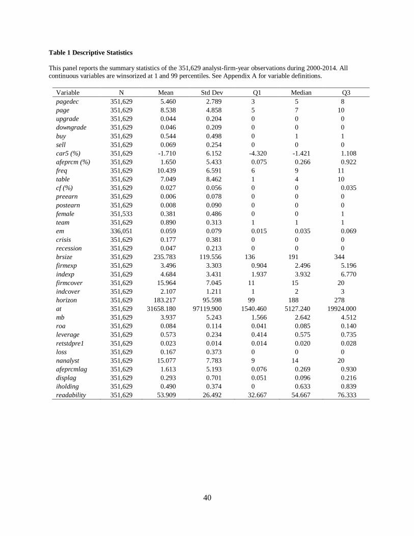
40

Table 1 Descriptive Statistics

This panel reports the summary statistics of the 351,629 analyst-firm-year observations during 2000-2014. All

continuous variables are winsorized at 1 and 99 percentiles. See Appendix A for variable definitions.

Variable N Mean Std Dev Q1 Median Q3

pagedec 351,629 5.460 2.789 3 5 8

page 351,629 8.538 4.858 5 7 10

upgrade 351,629 0.044 0.204 0 0 0

downgrade 351,629 0.046 0.209 0 0 0

buy 351,629 0.544 0.498 0 1 1

sell 351,629 0.069 0.254 0 0 0

car5 (%) 351,629 -1.710 6.152 -4.320 -1.421 1.108

afeprcm (%) 351,629 1.650 5.433 0.075 0.266 0.922

freq 351,629 10.439 6.591 6 9 11

table 351,629 7.049 8.462 1 4 10

cf (%) 351,629 0.027 0.056 0 0 0.035

preearn 351,629 0.006 0.078 0 0 0

postearn 351,629 0.008 0.090 0 0 0

female 351,533 0.381 0.486 0 0 1

team 351,629 0.890 0.313 1 1 1

em 336,051 0.059 0.079 0.015 0.035 0.069

crisis 351,629 0.177 0.381 0 0 0

recession 351,629 0.047 0.213 0 0 0

brsize 351,629 235.783 119.556 136 191 344

firmexp 351,629 3.496 3.303 0.904 2.496 5.196

indexp 351,629 4.684 3.431 1.937 3.932 6.770

firmcover 351,629 15.964 7.045 11 15 20

indcover 351,629 2.107 1.211 1 2 3

horizon 351,629 183.217 95.598 99 188 278

at 351,629 31658.180 97119.900 1540.460 5127.240 19924.000

mb 351,629 3.937 5.243 1.566 2.642 4.512

roa 351,629 0.084 0.114 0.041 0.085 0.140

leverage 351,629 0.573 0.234 0.414 0.575 0.735

retstdpre1 351,629 0.023 0.014 0.014 0.020 0.028

loss 351,629 0.167 0.373 0 0 0

nanalyst 351,629 15.077 7.783 9 14 20

afeprcmlag 351,629 1.613 5.193 0.076 0.269 0.930

displag 351,629 0.293 0.701 0.051 0.096 0.216

iholding 351,629 0.490 0.374 0 0.633 0.839

readability 351,629 53.909 26.492 32.667 54.667 76.333

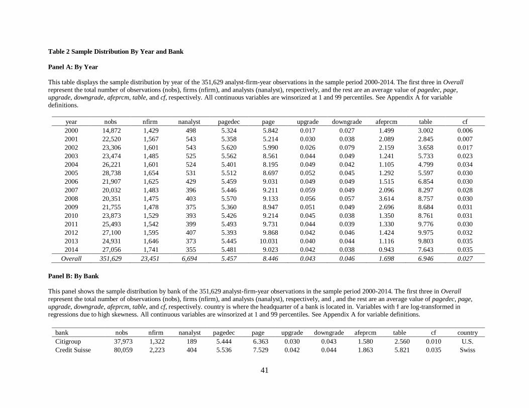
41

Table 2 Sample Distribution By Year and Bank

Panel A: By Year

This table displays the sample distribution by year of the 351,629 analyst-firm-year observations in the sample period 2000-2014. The first three in Overall

represent the total number of observations (nobs), firms (nfirm), and analysts (nanalyst), respectively, and the rest are an average value of pagedec, page, upgrade, downgrade, afeprcm, table, and cf, respectively. All continuous variables are winsorized at 1 and 99 percentiles. See Appendix A for variable

definitions.

year nobs nfirm nanalyst pagedec page upgrade downgrade afeprcm table cf

2000 14,872 1,429 498 5.324 5.842 0.017 0.027 1.499 3.002 0.006

2001 22,520 1,567 543 5.358 5.214 0.030 0.038 2.089 2.845 0.007

2002 23,306 1,601 543 5.620 5.990 0.026 0.079 2.159 3.658 0.017

2003 23,474 1,485 525 5.562 8.561 0.044 0.049 1.241 5.733 0.023

2004 26,221 1,601 524 5.401 8.195 0.049 0.042 1.105 4.799 0.034

2005 28,738 1,654 531 5.512 8.697 0.052 0.045 1.292 5.597 0.030

2006 21,907 1,625 429 5.459 9.031 0.049 0.049 1.515 6.854 0.030

2007 20,032 1,483 396 5.446 9.211 0.059 0.049 2.096 8.297 0.028

2008 20,351 1,475 403 5.570 9.133 0.056 0.057 3.614 8.757 0.030

2009 21,755 1,478 375 5.360 8.947 0.051 0.049 2.696 8.684 0.031

2010 23,873 1,529 393 5.426 9.214 0.045 0.038 1.350 8.761 0.031

2011 25,493 1,542 399 5.493 9.731 0.044 0.039 1.330 9.776 0.030

2012 27,100 1,595 407 5.393 9.868 0.042 0.046 1.424 9.975 0.032

2013 24,931 1,646 373 5.445 10.031 0.040 0.044 1.116 9.803 0.035

2014 27,056 1,741 355 5.481 9.023 0.042 0.038 0.943 7.643 0.035

Overall 351,629 23,451 6,694 5.457 8.446 0.043 0.046 1.698 6.946 0.027

Panel B: By Bank

This panel shows the sample distribution by bank of the 351,629 analyst-firm-year observations in the sample period 2000-2014. The first three in Overall

represent the total number of observations (nobs), firms (nfirm), and analysts (nanalyst), respectively, and , and the rest are an average value of pagedec, page,

upgrade, downgrade, afeprcm, table, and cf, respectively. country is where the headquarter of a bank is located in. Variables with ϯ are log-transformed in

regressions due to high skewness. All continuous variables are winsorized at 1 and 99 percentiles. See Appendix A for variable definitions.

bank nobs nfirm nanalyst pagedec page upgrade downgrade afeprcm table cf country

Citigroup 37,973 1,322 189 5.444 6.363 0.030 0.043 1.580 2.560 0.010 U.S.

Credit Suisse 80,059 2,223 404 5.536 7.529 0.042 0.044 1.863 5.821 0.035 Swiss

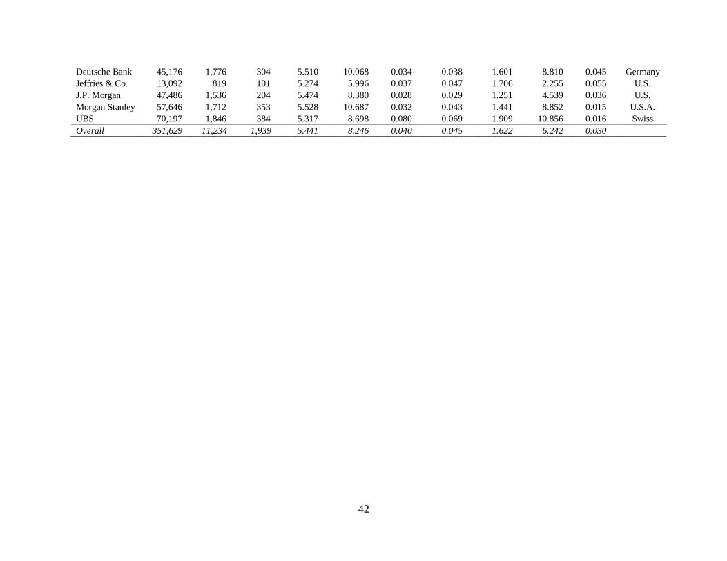
42

Deutsche Bank 45,176 1,776 304 5.510 10.068 0.034 0.038 1.601 8.810 0.045 Germany

Jeffries & Co. 13,092 819 101 5.274 5.996 0.037 0.047 1.706 2.255 0.055 U.S.

J.P. Morgan 47,486 1,536 204 5.474 8.380 0.028 0.029 1.251 4.539 0.036 U.S.

Morgan Stanley 57,646 1,712 353 5.528 10.687 0.032 0.043 1.441 8.852 0.015 U.S.A.

UBS 70,197 1,846 384 5.317 8.698 0.080 0.069 1.909 10.856 0.016 Swiss

Overall 351,629 11,234 1,939 5.441 8.246 0.040 0.045 1.622 6.242 0.030

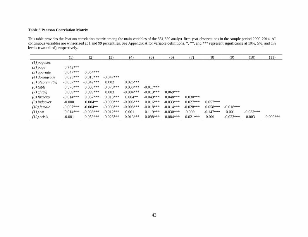
43

Table 3 Pearson Correlation Matrix

This table provides the Pearson correlation matrix among the main variables of the 351,629 analyst-firm-year observations in the sample period 2000-2014. All

continuous variables are winsorized at 1 and 99 percentiles. See Appendix A for variable definitions. *, **, and *** represent significance at 10%, 5%, and 1%

levels (two-tailed), respectively.

(1) (2) (3) (4) (5) (6) (7) (8) (9) (10) (11)

(1) pagedec

(2) page 0.742***

(3) upgrade 0.047*** 0.054***

(4) downgrade 0.023*** 0.013*** -0.047***

(5) afeprcm (%) -0.037*** -0.042*** 0.002 0.026***

(6) table 0.576*** 0.808*** 0.070*** 0.030*** -0.017***

(7) cf (%) 0.089*** 0.099*** 0.003 -0.004*** -0.013*** 0.069***

(8) firmexp -0.014*** 0.067*** 0.013*** 0.004** -0.049*** 0.048*** 0.030***

(9) indcover -0.000 0.004** -0.009*** -0.006*** 0.016*** -0.033*** 0.027*** 0.057***

(10) female -0.007*** -0.004** -0.008*** -0.008*** -0.018*** -0.014*** -0.028*** 0.058*** -0.018***

(11) em 0.014*** -0.036*** -0.012*** 0.001 0.119*** -0.030*** 0.000 -0.147*** 0.001 -0.033***

(12) crisis -0.001 0.053*** 0.026*** 0.013*** 0.098*** 0.084*** 0.021*** 0.001 -0.023*** 0.003 0.009***

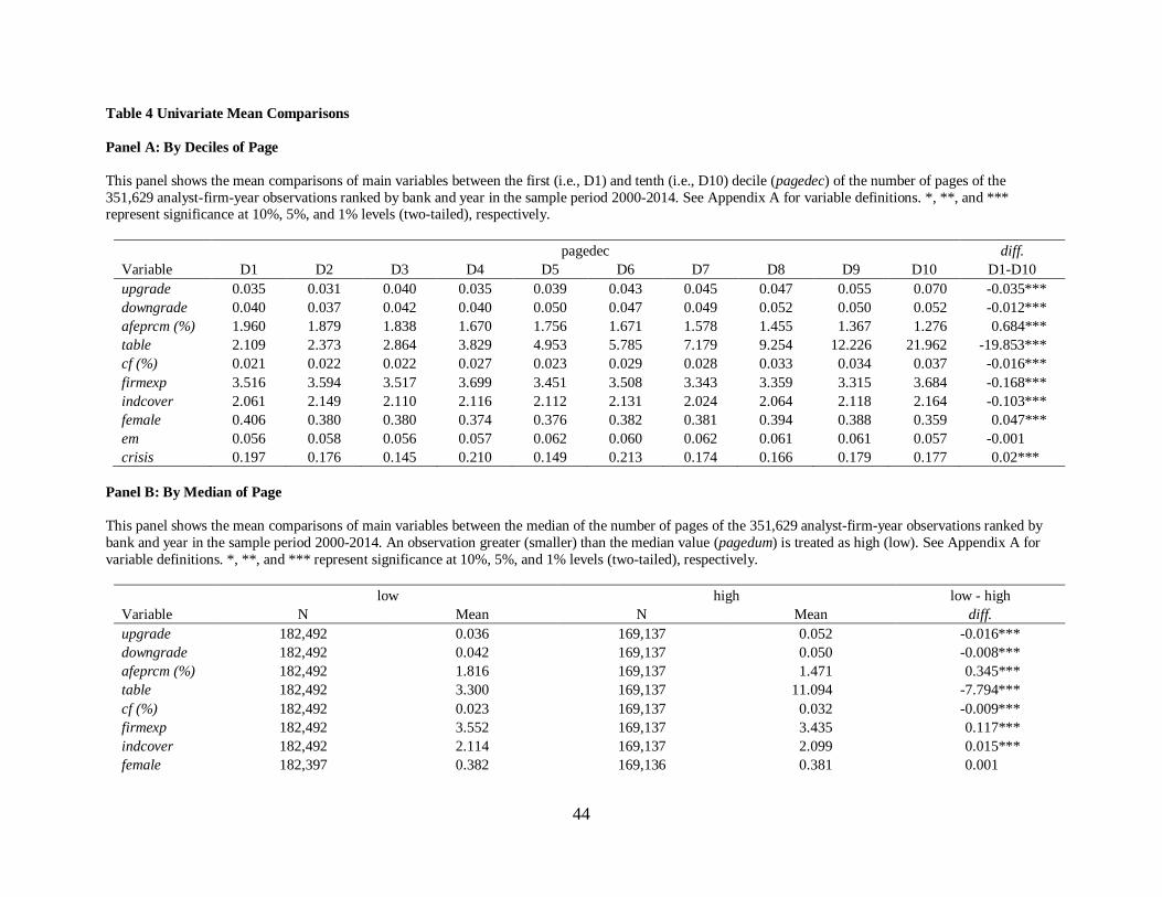
44

Table 4 Univariate Mean Comparisons

Panel A: By Deciles of Page

This panel shows the mean comparisons of main variables between the first (i.e., D1) and tenth (i.e., D10) decile (pagedec) of the number of pages of the

351,629 analyst-firm-year observations ranked by bank and year in the sample period 2000-2014. See Appendix A for variable definitions. *, **, and ***

represent significance at 10%, 5%, and 1% levels (two-tailed), respectively.

pagedec diff.

Variable D1 D2 D3 D4 D5 D6 D7 D8 D9 D10 D1-D10

upgrade 0.035 0.031 0.040 0.035 0.039 0.043 0.045 0.047 0.055 0.070 -0.035***

downgrade 0.040 0.037 0.042 0.040 0.050 0.047 0.049 0.052 0.050 0.052 -0.012***

afeprcm (%) 1.960 1.879 1.838 1.670 1.756 1.671 1.578 1.455 1.367 1.276 0.684***

table 2.109 2.373 2.864 3.829 4.953 5.785 7.179 9.254 12.226 21.962 -19.853***

cf (%) 0.021 0.022 0.022 0.027 0.023 0.029 0.028 0.033 0.034 0.037 -0.016***

firmexp 3.516 3.594 3.517 3.699 3.451 3.508 3.343 3.359 3.315 3.684 -0.168***

indcover 2.061 2.149 2.110 2.116 2.112 2.131 2.024 2.064 2.118 2.164 -0.103***

female 0.406 0.380 0.380 0.374 0.376 0.382 0.381 0.394 0.388 0.359 0.047***

em 0.056 0.058 0.056 0.057 0.062 0.060 0.062 0.061 0.061 0.057 -0.001

crisis 0.197 0.176 0.145 0.210 0.149 0.213 0.174 0.166 0.179 0.177 0.02***

Panel B: By Median of Page

This panel shows the mean comparisons of main variables between the median of the number of pages of the 351,629 analyst-firm-year observations ranked by

bank and year in the sample period 2000-2014. An observation greater (smaller) than the median value (pagedum) is treated as high (low). See Appendix A for

variable definitions. *, **, and *** represent significance at 10%, 5%, and 1% levels (two-tailed), respectively.

low high low - high

Variable N Mean N Mean diff.

upgrade 182,492 0.036 169,137 0.052 -0.016***

downgrade 182,492 0.042 169,137 0.050 -0.008***

afeprcm (%) 182,492 1.816 169,137 1.471 0.345***

table 182,492 3.300 169,137 11.094 -7.794***

cf (%) 182,492 0.023 169,137 0.032 -0.009***

firmexp 182,492 3.552 169,137 3.435 0.117***

indcover 182,492 2.114 169,137 2.099 0.015***

female 182,397 0.382 169,136 0.381 0.001

45

em 174,746 0.058 161,305 0.060 -0.002***

crisis 182,492 0.172 169,137 0.182 -0.010***

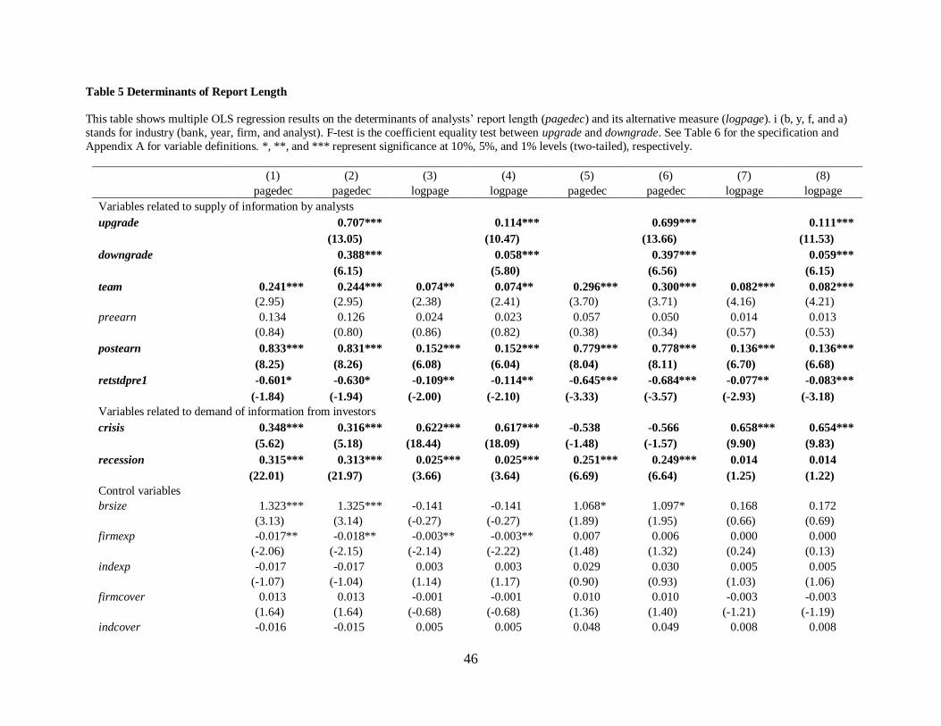
46

Table 5 Determinants of Report Length

This table shows multiple OLS regression results on the determinants of analysts’ report length (pagedec) and its alternative measure (logpage). i (b, y, f, and a)

stands for industry (bank, year, firm, and analyst). F-test is the coefficient equality test between upgrade and downgrade. See Table 6 for the specification and

Appendix A for variable definitions. *, **, and *** represent significance at 10%, 5%, and 1% levels (two-tailed), respectively.

(1) (2) (3) (4) (5) (6) (7) (8)

pagedec pagedec logpage logpage pagedec pagedec logpage logpage

Variables related to supply of information by analysts

upgrade 0.707*** 0.114*** 0.699*** 0.111***

(13.05) (10.47) (13.66) (11.53)

downgrade 0.388*** 0.058*** 0.397*** 0.059***

(6.15) (5.80) (6.56) (6.15)

team 0.241*** 0.244*** 0.074** 0.074** 0.296*** 0.300*** 0.082*** 0.082***

(2.95) (2.95) (2.38) (2.41) (3.70) (3.71) (4.16) (4.21)

preearn 0.134 0.126 0.024 0.023 0.057 0.050 0.014 0.013

(0.84) (0.80) (0.86) (0.82) (0.38) (0.34) (0.57) (0.53)

postearn 0.833*** 0.831*** 0.152*** 0.152*** 0.779*** 0.778*** 0.136*** 0.136***

(8.25) (8.26) (6.08) (6.04) (8.04) (8.11) (6.70) (6.68)

retstdpre1 -0.601* -0.630* -0.109** -0.114** -0.645*** -0.684*** -0.077** -0.083***

(-1.84) (-1.94) (-2.00) (-2.10) (-3.33) (-3.57) (-2.93) (-3.18)

Variables related to demand of information from investors

crisis 0.348*** 0.316*** 0.622*** 0.617*** -0.538 -0.566 0.658*** 0.654***

(5.62) (5.18) (18.44) (18.09) (-1.48) (-1.57) (9.90) (9.83)

recession 0.315*** 0.313*** 0.025*** 0.025*** 0.251*** 0.249*** 0.014 0.014

(22.01) (21.97) (3.66) (3.64) (6.69) (6.64) (1.25) (1.22)

Control variables

brsize 1.323*** 1.325*** -0.141 -0.141 1.068* 1.097* 0.168 0.172

(3.13) (3.14) (-0.27) (-0.27) (1.89) (1.95) (0.66) (0.69)

firmexp -0.017** -0.018** -0.003** -0.003** 0.007 0.006 0.000 0.000

(-2.06) (-2.15) (-2.14) (-2.22) (1.48) (1.32) (0.24) (0.13)

indexp -0.017 -0.017 0.003 0.003 0.029 0.030 0.005 0.005

(-1.07) (-1.04) (1.14) (1.17) (0.90) (0.93) (1.03) (1.06)

firmcover 0.013 0.013 -0.001 -0.001 0.010 0.010 -0.003 -0.003

(1.64) (1.64) (-0.68) (-0.68) (1.36) (1.40) (-1.21) (-1.19)

indcover -0.016 -0.015 0.005 0.005 0.048 0.049 0.008 0.008

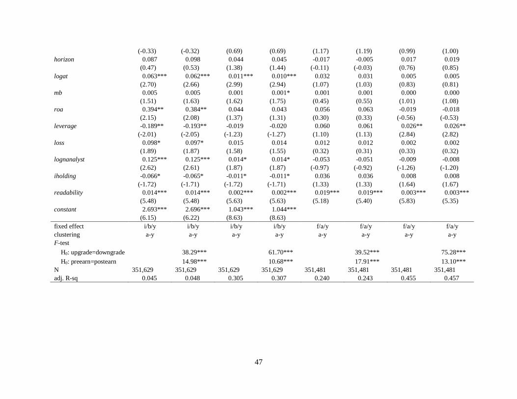
47

(-0.33) (-0.32) (0.69) (0.69) (1.17) (1.19) (0.99) (1.00)

horizon 0.087 0.098 0.044 0.045 -0.017 -0.005 0.017 0.019

(0.47) (0.53) (1.38) (1.44) (-0.11) (-0.03) (0.76) (0.85)

logat 0.063*** 0.062*** 0.011*** 0.010*** 0.032 0.031 0.005 0.005

(2.70) (2.66) (2.99) (2.94) (1.07) (1.03) (0.83) (0.81)

mb 0.005 0.005 0.001 0.001* 0.001 0.001 0.000 0.000

(1.51) (1.63) (1.62) (1.75) (0.45) (0.55) (1.01) (1.08)

roa 0.394** 0.384** 0.044 0.043 0.056 0.063 -0.019 -0.018

(2.15) (2.08) (1.37) (1.31) (0.30) (0.33) (-0.56) (-0.53)

leverage -0.189** -0.193** -0.019 -0.020 0.060 0.061 0.026** 0.026**

(-2.01) (-2.05) (-1.23) (-1.27) (1.10) (1.13) (2.84) (2.82)

loss 0.098* 0.097* 0.015 0.014 0.012 0.012 0.002 0.002

(1.89) (1.87) (1.58) (1.55) (0.32) (0.31) (0.33) (0.32)

lognanalyst 0.125*** 0.125*** 0.014* 0.014* -0.053 -0.051 -0.009 -0.008

(2.62) (2.61) (1.87) (1.87) (-0.97) (-0.92) (-1.26) (-1.20)

iholding -0.066* -0.065* -0.011* -0.011* 0.036 0.036 0.008 0.008

(-1.72) (-1.71) (-1.72) (-1.71) (1.33) (1.33) (1.64) (1.67)

readability 0.014*** 0.014*** 0.002*** 0.002*** 0.019*** 0.019*** 0.003*** 0.003***

(5.48) (5.48) (5.63) (5.63) (5.18) (5.40) (5.83) (5.35)

constant 2.693*** 2.696*** 1.043*** 1.044***

(6.15) (6.22) (8.63) (8.63)

fixed effect i/b/y i/b/y i/b/y i/b/y f/a/y f/a/y f/a/y f/a/y

clustering a-y a-y a-y a-y a-y a-y a-y a-y

F-test

H0: upgrade=downgrade 38.29*** 61.70*** 39.52*** 75.28***

H0: preearn=postearn 14.98*** 10.68*** 17.91*** 13.10***

N 351,629 351,629 351,629 351,629 351,481 351,481 351,481 351,481

adj. R-sq 0.045 0.048 0.305 0.307 0.240 0.243 0.455 0.457

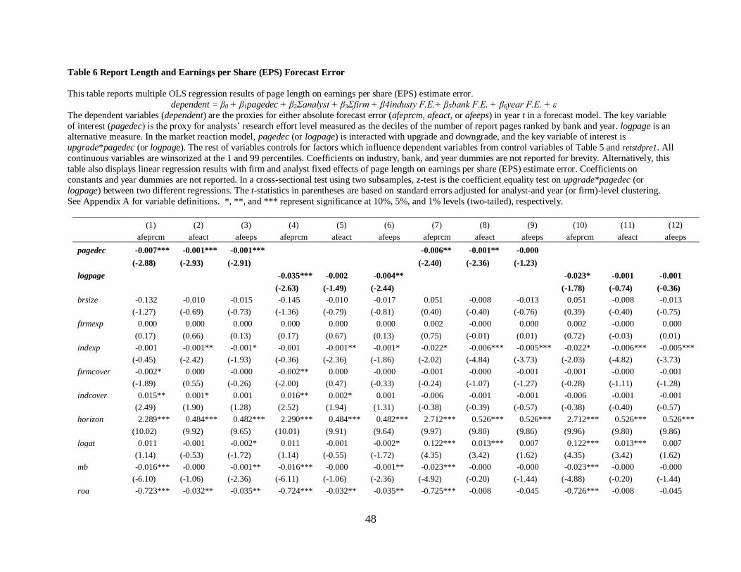
48

Table 6 Report Length and Earnings per Share (EPS) Forecast Error

This table reports multiple OLS regression results of page length on earnings per share (EPS) estimate error.

dependent = β0 + β1pagedec + β2Σanalyst + β3Σfirm + β4industy F.E.+ β5bank F.E. + β6year F.E. + ε

The dependent variables (dependent) are the proxies for either absolute forecast error (afeprcm, afeact, or afeeps) in year t in a forecast model. The key variable

of interest (pagedec) is the proxy for analysts’ research effort level measured as the deciles of the number of report pages ranked by bank and year. logpage is an alternative measure. In the market reaction model, pagedec (or logpage) is interacted with upgrade and downgrade, and the key variable of interest is

upgrade*pagedec (or logpage). The rest of variables controls for factors which influence dependent variables from control variables of Table 5 and retstdpre1. All

continuous variables are winsorized at the 1 and 99 percentiles. Coefficients on industry, bank, and year dummies are not reported for brevity. Alternatively, this

table also displays linear regression results with firm and analyst fixed effects of page length on earnings per share (EPS) estimate error. Coefficients on

constants and year dummies are not reported. In a cross-sectional test using two subsamples, z-test is the coefficient equality test on upgrade*pagedec (or

logpage) between two different regressions. The t-statistics in parentheses are based on standard errors adjusted for analyst-and year (or firm)-level clustering.

See Appendix A for variable definitions. *, **, and *** represent significance at 10%, 5%, and 1% levels (two-tailed), respectively.

(1) (2) (3) (4) (5) (6) (7) (8) (9) (10) (11) (12)

afeprcm afeact afeeps afeprcm afeact afeeps afeprcm afeact afeeps afeprcm afeact afeeps

pagedec -0.007*** -0.001*** -0.001*** -0.006** -0.001** -0.000

(-2.88) (-2.93) (-2.91) (-2.40) (-2.36) (-1.23)

logpage -0.035*** -0.002 -0.004** -0.023* -0.001 -0.001

(-2.63) (-1.49) (-2.44) (-1.78) (-0.74) (-0.36)

brsize -0.132 -0.010 -0.015 -0.145 -0.010 -0.017 0.051 -0.008 -0.013 0.051 -0.008 -0.013

(-1.27) (-0.69) (-0.73) (-1.36) (-0.79) (-0.81) (0.40) (-0.40) (-0.76) (0.39) (-0.40) (-0.75)

firmexp 0.000 0.000 0.000 0.000 0.000 0.000 0.002 -0.000 0.000 0.002 -0.000 0.000

(0.17) (0.66) (0.13) (0.17) (0.67) (0.13) (0.75) (-0.01) (0.01) (0.72) (-0.03) (0.01)

indexp -0.001 -0.001** -0.001* -0.001 -0.001** -0.001* -0.022* -0.006*** -0.005*** -0.022* -0.006*** -0.005***

(-0.45) (-2.42) (-1.93) (-0.36) (-2.36) (-1.86) (-2.02) (-4.84) (-3.73) (-2.03) (-4.82) (-3.73)

firmcover -0.002* 0.000 -0.000 -0.002** 0.000 -0.000 -0.001 -0.000 -0.001 -0.001 -0.000 -0.001

(-1.89) (0.55) (-0.26) (-2.00) (0.47) (-0.33) (-0.24) (-1.07) (-1.27) (-0.28) (-1.11) (-1.28)

indcover 0.015** 0.001* 0.001 0.016** 0.002* 0.001 -0.006 -0.001 -0.001 -0.006 -0.001 -0.001

(2.49) (1.90) (1.28) (2.52) (1.94) (1.31) (-0.38) (-0.39) (-0.57) (-0.38) (-0.40) (-0.57)

horizon 2.289*** 0.484*** 0.482*** 2.290*** 0.484*** 0.482*** 2.712*** 0.526*** 0.526*** 2.712*** 0.526*** 0.526***

(10.02) (9.92) (9.65) (10.01) (9.91) (9.64) (9.97) (9.80) (9.86) (9.96) (9.80) (9.86)

logat 0.011 -0.001 -0.002* 0.011 -0.001 -0.002* 0.122*** 0.013*** 0.007 0.122*** 0.013*** 0.007

(1.14) (-0.53) (-1.72) (1.14) (-0.55) (-1.72) (4.35) (3.42) (1.62) (4.35) (3.42) (1.62)

mb -0.016*** -0.000 -0.001** -0.016*** -0.000 -0.001** -0.023*** -0.000 -0.000 -0.023*** -0.000 -0.000

(-6.10) (-1.06) (-2.36) (-6.11) (-1.06) (-2.36) (-4.92) (-0.20) (-1.44) (-4.88) (-0.20) (-1.44)

roa -0.723*** -0.032** -0.035** -0.724*** -0.032** -0.035** -0.725*** -0.008 -0.045 -0.726*** -0.008 -0.045

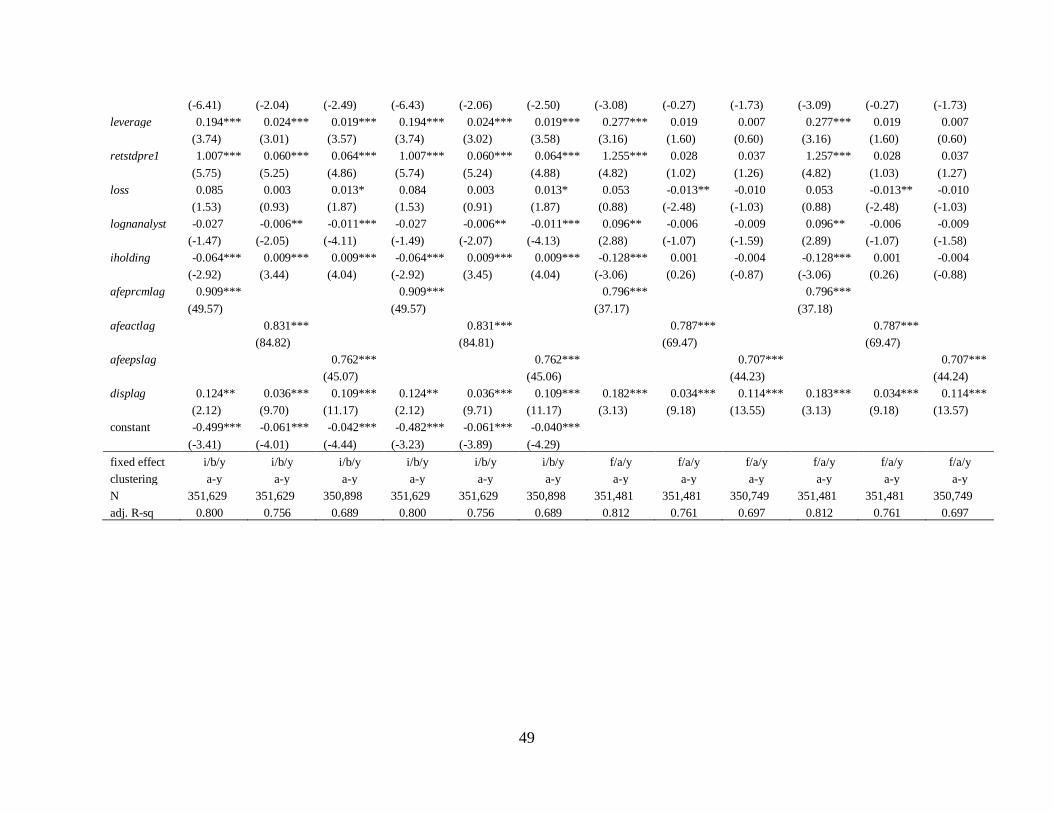
49

(-6.41) (-2.04) (-2.49) (-6.43) (-2.06) (-2.50) (-3.08) (-0.27) (-1.73) (-3.09) (-0.27) (-1.73)

leverage 0.194*** 0.024*** 0.019*** 0.194*** 0.024*** 0.019*** 0.277*** 0.019 0.007 0.277*** 0.019 0.007

(3.74) (3.01) (3.57) (3.74) (3.02) (3.58) (3.16) (1.60) (0.60) (3.16) (1.60) (0.60)

retstdpre1 1.007*** 0.060*** 0.064*** 1.007*** 0.060*** 0.064*** 1.255*** 0.028 0.037 1.257*** 0.028 0.037

(5.75) (5.25) (4.86) (5.74) (5.24) (4.88) (4.82) (1.02) (1.26) (4.82) (1.03) (1.27)

loss 0.085 0.003 0.013* 0.084 0.003 0.013* 0.053 -0.013** -0.010 0.053 -0.013** -0.010

(1.53) (0.93) (1.87) (1.53) (0.91) (1.87) (0.88) (-2.48) (-1.03) (0.88) (-2.48) (-1.03)

lognanalyst -0.027 -0.006** -0.011*** -0.027 -0.006** -0.011*** 0.096** -0.006 -0.009 0.096** -0.006 -0.009

(-1.47) (-2.05) (-4.11) (-1.49) (-2.07) (-4.13) (2.88) (-1.07) (-1.59) (2.89) (-1.07) (-1.58)

iholding -0.064*** 0.009*** 0.009*** -0.064*** 0.009*** 0.009*** -0.128*** 0.001 -0.004 -0.128*** 0.001 -0.004

(-2.92) (3.44) (4.04) (-2.92) (3.45) (4.04) (-3.06) (0.26) (-0.87) (-3.06) (0.26) (-0.88)

afeprcmlag 0.909*** 0.909*** 0.796*** 0.796***

(49.57) (49.57) (37.17) (37.18)

afeactlag 0.831*** 0.831*** 0.787*** 0.787***

(84.82) (84.81) (69.47) (69.47)

afeepslag 0.762*** 0.762*** 0.707*** 0.707***

(45.07) (45.06) (44.23) (44.24)

displag 0.124** 0.036*** 0.109*** 0.124** 0.036*** 0.109*** 0.182*** 0.034*** 0.114*** 0.183*** 0.034*** 0.114***

(2.12) (9.70) (11.17) (2.12) (9.71) (11.17) (3.13) (9.18) (13.55) (3.13) (9.18) (13.57)

constant -0.499*** -0.061*** -0.042*** -0.482*** -0.061*** -0.040***

(-3.41) (-4.01) (-4.44) (-3.23) (-3.89) (-4.29)

fixed effect i/b/y i/b/y i/b/y i/b/y i/b/y i/b/y f/a/y f/a/y f/a/y f/a/y f/a/y f/a/y

clustering a-y a-y a-y a-y a-y a-y a-y a-y a-y a-y a-y a-y

N 351,629 351,629 350,898 351,629 351,629 350,898 351,481 351,481 350,749 351,481 351,481 350,749

adj. R-sq 0.800 0.756 0.689 0.800 0.756 0.689 0.812 0.761 0.697 0.812 0.761 0.697

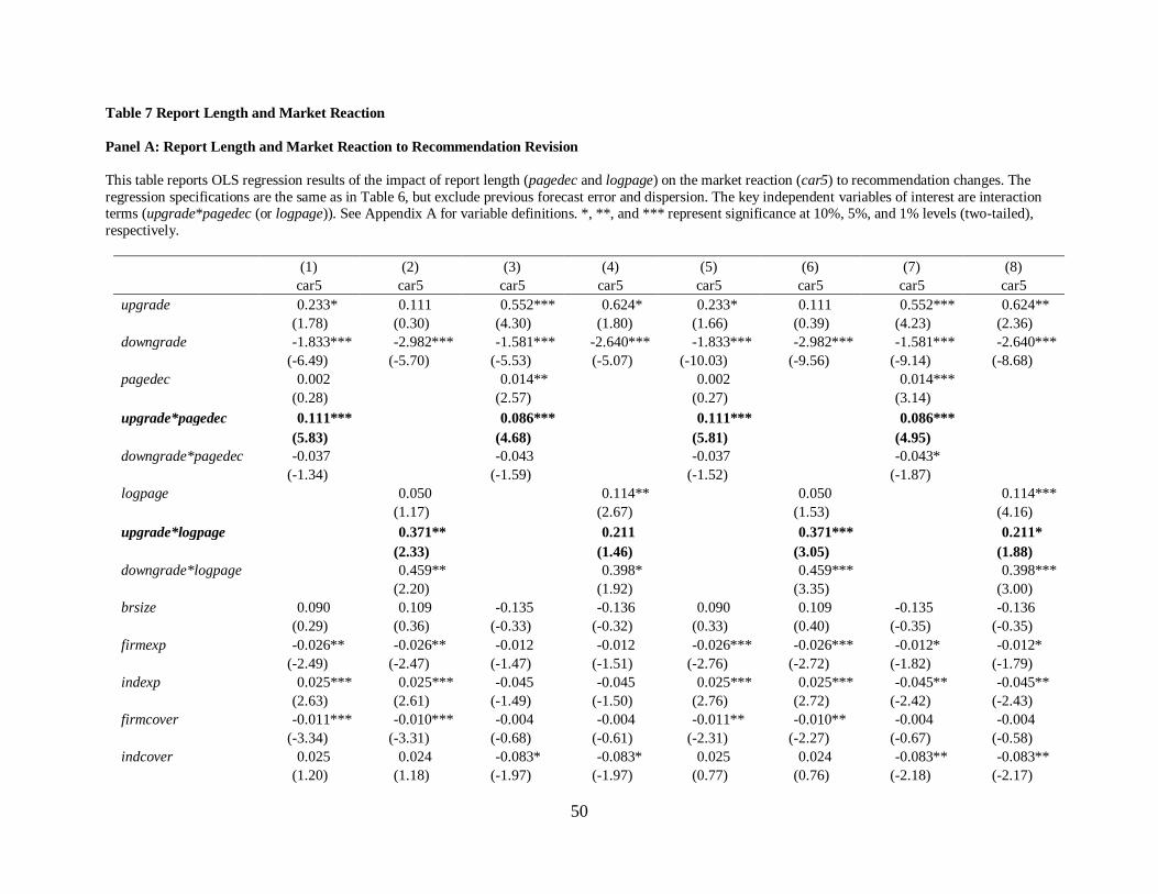
50

Table 7 Report Length and Market Reaction

Panel A: Report Length and Market Reaction to Recommendation Revision

This table reports OLS regression results of the impact of report length (pagedec and logpage) on the market reaction (car5) to recommendation changes. The

regression specifications are the same as in Table 6, but exclude previous forecast error and dispersion. The key independent variables of interest are interaction terms (upgrade*pagedec (or logpage)). See Appendix A for variable definitions. *, **, and *** represent significance at 10%, 5%, and 1% levels (two-tailed),

respectively.

(1) (2) (3) (4) (5) (6) (7) (8)

car5 car5 car5 car5 car5 car5 car5 car5

upgrade 0.233* 0.111 0.552*** 0.624* 0.233* 0.111 0.552*** 0.624**

(1.78) (0.30) (4.30) (1.80) (1.66) (0.39) (4.23) (2.36)

downgrade -1.833*** -2.982*** -1.581*** -2.640*** -1.833*** -2.982*** -1.581*** -2.640***

(-6.49) (-5.70) (-5.53) (-5.07) (-10.03) (-9.56) (-9.14) (-8.68)

pagedec 0.002 0.014** 0.002 0.014***

(0.28) (2.57) (0.27) (3.14)

upgrade*pagedec 0.111*** 0.086*** 0.111*** 0.086***

(5.83) (4.68) (5.81) (4.95)

downgrade*pagedec -0.037 -0.043 -0.037 -0.043*

(-1.34) (-1.59) (-1.52) (-1.87)

logpage 0.050 0.114** 0.050 0.114***

(1.17) (2.67) (1.53) (4.16)

upgrade*logpage 0.371** 0.211 0.371*** 0.211*

(2.33) (1.46) (3.05) (1.88)

downgrade*logpage 0.459** 0.398* 0.459*** 0.398***

(2.20) (1.92) (3.35) (3.00)

brsize 0.090 0.109 -0.135 -0.136 0.090 0.109 -0.135 -0.136

(0.29) (0.36) (-0.33) (-0.32) (0.33) (0.40) (-0.35) (-0.35)

firmexp -0.026** -0.026** -0.012 -0.012 -0.026*** -0.026*** -0.012* -0.012*

(-2.49) (-2.47) (-1.47) (-1.51) (-2.76) (-2.72) (-1.82) (-1.79)

indexp 0.025*** 0.025*** -0.045 -0.045 0.025*** 0.025*** -0.045** -0.045**

(2.63) (2.61) (-1.49) (-1.50) (2.76) (2.72) (-2.42) (-2.43)

firmcover -0.011*** -0.010*** -0.004 -0.004 -0.011** -0.010** -0.004 -0.004

(-3.34) (-3.31) (-0.68) (-0.61) (-2.31) (-2.27) (-0.67) (-0.58)

indcover 0.025 0.024 -0.083* -0.083* 0.025 0.024 -0.083** -0.083**

(1.20) (1.18) (-1.97) (-1.97) (0.77) (0.76) (-2.18) (-2.17)

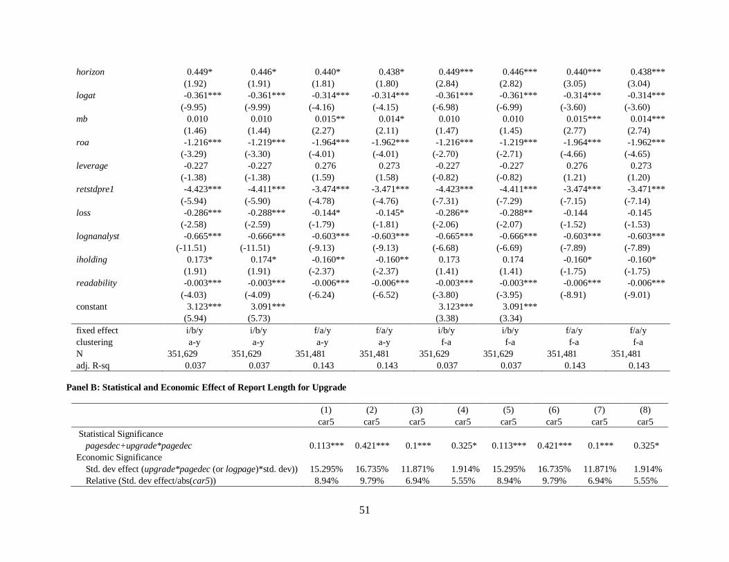
51

horizon 0.449* 0.446* 0.440* 0.438* 0.449*** 0.446*** 0.440*** 0.438***

(1.92) (1.91) (1.81) (1.80) (2.84) (2.82) (3.05) (3.04)

logat -0.361*** -0.361*** -0.314*** -0.314*** -0.361*** -0.361*** -0.314*** -0.314***

(-9.95) (-9.99) (-4.16) (-4.15) (-6.98) (-6.99) (-3.60) (-3.60)

mb 0.010 0.010 0.015** 0.014* 0.010 0.010 0.015*** 0.014***

(1.46) (1.44) (2.27) (2.11) (1.47) (1.45) (2.77) (2.74)

roa -1.216*** -1.219*** -1.964*** -1.962*** -1.216*** -1.219*** -1.964*** -1.962***

(-3.29) (-3.30) (-4.01) (-4.01) (-2.70) (-2.71) (-4.66) (-4.65)

leverage -0.227 -0.227 0.276 0.273 -0.227 -0.227 0.276 0.273

(-1.38) (-1.38) (1.59) (1.58) (-0.82) (-0.82) (1.21) (1.20)

retstdpre1 -4.423*** -4.411*** -3.474*** -3.471*** -4.423*** -4.411*** -3.474*** -3.471***

(-5.94) (-5.90) (-4.78) (-4.76) (-7.31) (-7.29) (-7.15) (-7.14)

loss -0.286*** -0.288*** -0.144* -0.145* -0.286** -0.288** -0.144 -0.145

(-2.58) (-2.59) (-1.79) (-1.81) (-2.06) (-2.07) (-1.52) (-1.53)

lognanalyst -0.665*** -0.666*** -0.603*** -0.603*** -0.665*** -0.666*** -0.603*** -0.603***

(-11.51) (-11.51) (-9.13) (-9.13) (-6.68) (-6.69) (-7.89) (-7.89)

iholding 0.173* 0.174* -0.160** -0.160** 0.173 0.174 -0.160* -0.160*

(1.91) (1.91) (-2.37) (-2.37) (1.41) (1.41) (-1.75) (-1.75)

readability -0.003*** -0.003*** -0.006*** -0.006*** -0.003*** -0.003*** -0.006*** -0.006***

(-4.03) (-4.09) (-6.24) (-6.52) (-3.80) (-3.95) (-8.91) (-9.01)

constant 3.123*** 3.091*** 3.123*** 3.091***

(5.94) (5.73) (3.38) (3.34)

fixed effect i/b/y i/b/y f/a/y f/a/y i/b/y i/b/y f/a/y f/a/y

clustering a-y a-y a-y a-y f-a f-a f-a f-a

N 351,629 351,629 351,481 351,481 351,629 351,629 351,481 351,481

adj. R-sq 0.037 0.037 0.143 0.143 0.037 0.037 0.143 0.143

Panel B: Statistical and Economic Effect of Report Length for Upgrade

(1) (2) (3) (4) (5) (6) (7) (8)

car5 car5 car5 car5 car5 car5 car5 car5

Statistical Significance

pagesdec+upgrade*pagedec 0.113*** 0.421*** 0.1*** 0.325* 0.113*** 0.421*** 0.1*** 0.325*

Economic Significance

Std. dev effect (upgrade*pagedec (or logpage)*std. dev)) 15.295% 16.735% 11.871% 1.914% 15.295% 16.735% 11.871% 1.914%

Relative (Std. dev effect/abs(car5)) 8.94% 9.79% 6.94% 5.55% 8.94% 9.79% 6.94% 5.55%

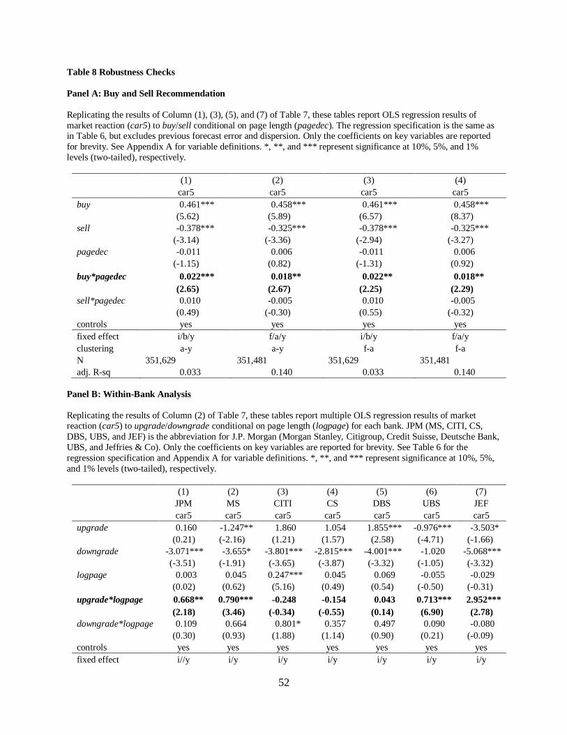
52

Table 8 Robustness Checks

Panel A: Buy and Sell Recommendation

Replicating the results of Column (1), (3), (5), and (7) of Table 7, these tables report OLS regression results of

market reaction (car5) to buy/sell conditional on page length (pagedec). The regression specification is the same as in Table 6, but excludes previous forecast error and dispersion. Only the coefficients on key variables are reported

for brevity. See Appendix A for variable definitions. *, **, and *** represent significance at 10%, 5%, and 1%

levels (two-tailed), respectively.

(1) (2) (3) (4)

car5 car5 car5 car5

buy 0.461*** 0.458*** 0.461*** 0.458***

(5.62) (5.89) (6.57) (8.37)

sell -0.378*** -0.325*** -0.378*** -0.325***

(-3.14) (-3.36) (-2.94) (-3.27)

pagedec -0.011 0.006 -0.011 0.006

(-1.15) (0.82) (-1.31) (0.92)

buy*pagedec 0.022*** 0.018** 0.022** 0.018**

(2.65) (2.67) (2.25) (2.29)

sell*pagedec 0.010 -0.005 0.010 -0.005

(0.49) (-0.30) (0.55) (-0.32)

controls yes yes yes yes

fixed effect i/b/y f/a/y i/b/y f/a/y

clustering a-y a-y f-a f-a

N 351,629 351,481 351,629 351,481

adj. R-sq 0.033 0.140 0.033 0.140

Panel B: Within-Bank Analysis

Replicating the results of Column (2) of Table 7, these tables report multiple OLS regression results of market reaction (car5) to upgrade/downgrade conditional on page length (logpage) for each bank. JPM (MS, CITI, CS,

DBS, UBS, and JEF) is the abbreviation for J.P. Morgan (Morgan Stanley, Citigroup, Credit Suisse, Deutsche Bank,

UBS, and Jeffries & Co). Only the coefficients on key variables are reported for brevity. See Table 6 for the

regression specification and Appendix A for variable definitions. *, **, and *** represent significance at 10%, 5%,

and 1% levels (two-tailed), respectively.

(1) (2) (3) (4) (5) (6) (7)

JPM MS CITI CS DBS UBS JEF

car5 car5 car5 car5 car5 car5 car5

upgrade 0.160 -1.247** 1.860 1.054 1.855*** -0.976*** -3.503*

(0.21) (-2.16) (1.21) (1.57) (2.58) (-4.71) (-1.66)

downgrade -3.071*** -3.655* -3.801*** -2.815*** -4.001*** -1.020 -5.068***

(-3.51) (-1.91) (-3.65) (-3.87) (-3.32) (-1.05) (-3.32)

logpage 0.003 0.045 0.247*** 0.045 0.069 -0.055 -0.029

(0.02) (0.62) (5.16) (0.49) (0.54) (-0.50) (-0.31)

upgrade*logpage 0.668** 0.790*** -0.248 -0.154 0.043 0.713*** 2.952***

(2.18) (3.46) (-0.34) (-0.55) (0.14) (6.90) (2.78)

downgrade*logpage 0.109 0.664 0.801* 0.357 0.497 0.090 -0.080

(0.30) (0.93) (1.88) (1.14) (0.90) (0.21) (-0.09)

controls yes yes yes yes yes yes yes

fixed effect i//y i/y i/y i/y i/y i/y i/y

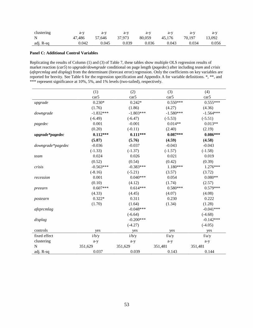
53

clustering a-y a-y a-y a-y a-y a-y a-y

N 47,486 57,646 37,973 80,059 45,176 70,197 13,092

adj. R-sq 0.042 0.045 0.039 0.036 0.043 0.034 0.056

Panel C: Additional Control Variables

Replicating the results of Column (1) and (3) of Table 7, these tables show multiple OLS regression results of

market reaction (car5) to upgrade/downgrade conditional on page length (pagedec) after including team and crisis

(afeprcmlag and displag) from the determinant (forecast error) regression. Only the coefficients on key variables are

reported for brevity. See Table 6 for the regression specification and Appendix A for variable definitions. *, **, and

*** represent significance at 10%, 5%, and 1% levels (two-tailed), respectively.

(1) (2) (3) (4)

car5 car5 car5 car5

upgrade 0.230* 0.242* 0.550*** 0.555***

(1.76) (1.86) (4.27) (4.36)

downgrade -1.832*** -1.803*** -1.580*** -1.564***

(-6.49) (-6.47) (-5.53) (-5.51)

pagedec 0.001 -0.001 0.014** 0.013**

(0.20) (-0.11) (2.40) (2.19)

upgrade*pagedec 0.112*** 0.111*** 0.087*** 0.086***

(5.87) (5.76) (4.59) (4.58)

downgrade*pagedec -0.036 -0.037 -0.043 -0.043

(-1.33) (-1.37) (-1.57) (-1.58)

team 0.024 0.026 0.021 0.019

(0.52) (0.54) (0.42) (0.39)

crisis -0.563*** -0.383*** 1.180*** 1.276***

(-8.16) (-5.21) (3.57) (3.72)

recession 0.001 0.040*** 0.054 0.080**

(0.10) (4.12) (1.74) (2.57)

preearn 0.607*** 0.614*** 0.580*** 0.579***

(4.33) (4.45) (4.07) (4.08)

postearn 0.322* 0.311 0.230 0.222

(1.70) (1.64) (1.34) (1.28)

afeprcmlag -0.048*** -0.041***

(-6.64) (-4.68)

displag -0.200*** -0.142***

(-4.27) (-4.05)

controls yes yes yes yes

fixed effect i/b/y i/b/y f/a/y f/a/y

clustering a-y a-y a-y a-y

N 351,629 351,629 351,481 351,481

adj. R-sq 0.037 0.039 0.143 0.144

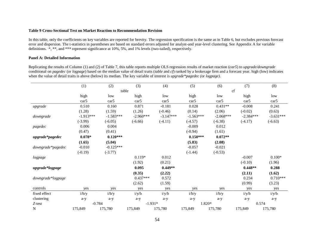
54

Table 9 Cross-Sectional Test on Market Reaction to Recommendation Revision

In this table, only the coefficients on key variables are reported for brevity. The regression specification is the same as in Table 6, but excludes previous forecast

error and dispersion. The t-statistics in parentheses are based on standard errors adjusted for analyst-and year-level clustering. See Appendix A for variable

definitions. *, **, and *** represent significance at 10%, 5%, and 1% levels (two-tailed), respectively.

Panel A: Detailed Information

Replicating the results of Column (1) and (2) of Table 7, this table reports multiple OLS regression results of market reaction (car5) to upgrade/downgrade

conditional on pagedec (or logpage) based on the median value of detail traits (table and cf) ranked by a brokerage firm and a forecast year. high (low) indicates

when the value of detail traits is above (below) its median. The key variable of interest is upgrade*pagedec (or logpage).

(1) (2) (3) (4) (5) (6) (7) (8)

table cf

high low high low high low high low

car5 car5 car5 car5 car5 car5 car5 car5

upgrade 0.510 0.160 0.871 -0.181 0.028 0.431** -0.008 0.241

(1.28) (1.59) (1.26) (-0.46) (0.14) (2.06) (-0.02) (0.63)

downgrade -1.913*** -1.583*** -2.960*** -3.147*** -1.563*** -2.068*** -2.384*** -3.631***

(-3.99) (-6.05) (-6.66) (-4.11) (-4.57) (-6.38) (-4.17) (-6.63)

pagedec 0.006 0.004 -0.009 0.012

(0.47) (0.41) (-0.94) (1.61)

upgrade*pagedec 0.078* 0.120*** 0.150*** 0.072**

(1.65) (5.04) (5.83) (2.08)

downgrade*pagedec -0.010 -0.125*** -0.057 -0.021

(-0.19) (-3.77) (-1.44) (-0.53)

logpage 0.119* 0.012 -0.007 0.100*

(1.92) (0.21) (-0.10) (1.96)

upgrade*logpage 0.095 0.449** 0.448** 0.288

(0.35) (2.22) (2.11) (1.62)

downgrade*logpage 0.437*** 0.572 0.234 0.710***

(2.62) (1.59) (0.99) (3.23)

controls yes yes yes yes yes yes yes yes

fixed effect i/b/y i/b/y i/y/b i/y/b i/b/y i/b/y i/y/b i/y/b

clustering a-y a-y a-y a-y a-y a-y a-y a-y

Z-test -0.784 -1.931* 1.820* 0.574

N 175,849 175,780 175,849 175,780 175,849 175,780 175,849 175,780

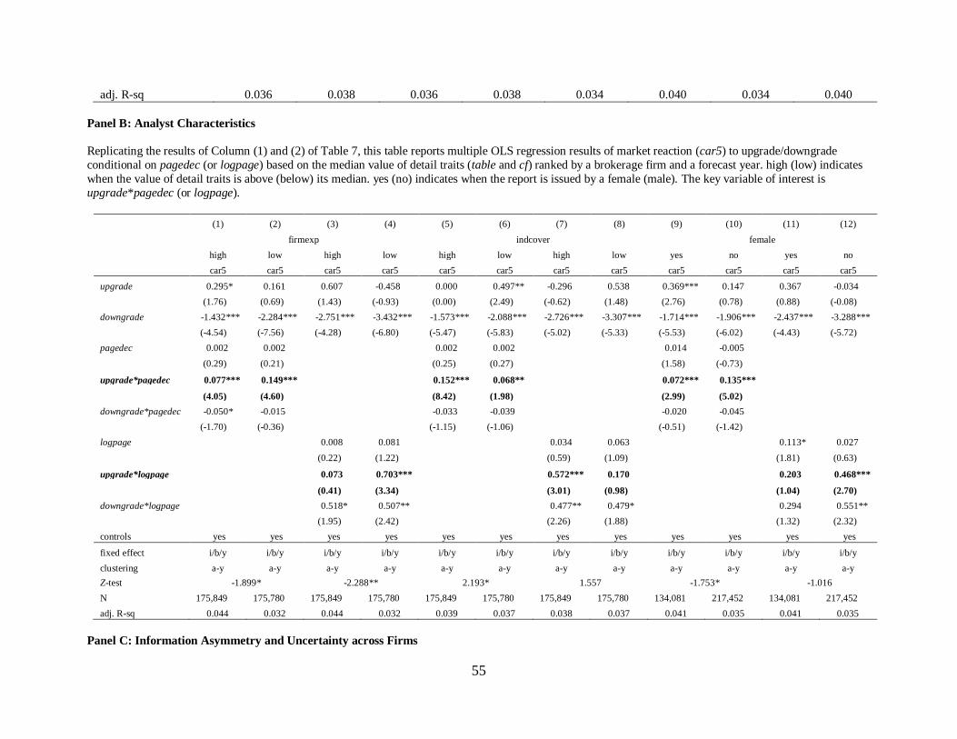
55

adj. R-sq 0.036 0.038 0.036 0.038 0.034 0.040 0.034 0.040

Panel B: Analyst Characteristics

Replicating the results of Column (1) and (2) of Table 7, this table reports multiple OLS regression results of market reaction (car5) to upgrade/downgrade

conditional on pagedec (or logpage) based on the median value of detail traits (table and cf) ranked by a brokerage firm and a forecast year. high (low) indicates

when the value of detail traits is above (below) its median. yes (no) indicates when the report is issued by a female (male). The key variable of interest is

upgrade*pagedec (or logpage).

(1) (2) (3) (4) (5) (6) (7) (8) (9) (10) (11) (12)

firmexp indcover female

high low high low high low high low yes no yes no

car5 car5 car5 car5 car5 car5 car5 car5 car5 car5 car5 car5

upgrade 0.295* 0.161 0.607 -0.458 0.000 0.497** -0.296 0.538 0.369*** 0.147 0.367 -0.034

(1.76) (0.69) (1.43) (-0.93) (0.00) (2.49) (-0.62) (1.48) (2.76) (0.78) (0.88) (-0.08)

downgrade -1.432*** -2.284*** -2.751*** -3.432*** -1.573*** -2.088*** -2.726*** -3.307*** -1.714*** -1.906*** -2.437*** -3.288***

(-4.54) (-7.56) (-4.28) (-6.80) (-5.47) (-5.83) (-5.02) (-5.33) (-5.53) (-6.02) (-4.43) (-5.72)

pagedec 0.002 0.002 0.002 0.002 0.014 -0.005

(0.29) (0.21) (0.25) (0.27) (1.58) (-0.73)

upgrade*pagedec 0.077*** 0.149*** 0.152*** 0.068** 0.072*** 0.135***

(4.05) (4.60) (8.42) (1.98) (2.99) (5.02)

downgrade*pagedec -0.050* -0.015 -0.033 -0.039 -0.020 -0.045

(-1.70) (-0.36) (-1.15) (-1.06) (-0.51) (-1.42)

logpage 0.008 0.081 0.034 0.063 0.113* 0.027

(0.22) (1.22) (0.59) (1.09) (1.81) (0.63)

upgrade*logpage 0.073 0.703*** 0.572*** 0.170 0.203 0.468***

(0.41) (3.34) (3.01) (0.98) (1.04) (2.70)

downgrade*logpage 0.518* 0.507** 0.477** 0.479* 0.294 0.551**

(1.95) (2.42) (2.26) (1.88) (1.32) (2.32)

controls yes yes yes yes yes yes yes yes yes yes yes yes

fixed effect i/b/y i/b/y i/b/y i/b/y i/b/y i/b/y i/b/y i/b/y i/b/y i/b/y i/b/y i/b/y

clustering a-y a-y a-y a-y a-y a-y a-y a-y a-y a-y a-y a-y

Z-test -1.899* -2.288** 2.193* 1.557 -1.753* -1.016

N 175,849 175,780 175,849 175,780 175,849 175,780 175,849 175,780 134,081 217,452 134,081 217,452

adj. R-sq 0.044 0.032 0.044 0.032 0.039 0.037 0.038 0.037 0.041 0.035 0.041 0.035

Panel C: Information Asymmetry and Uncertainty across Firms

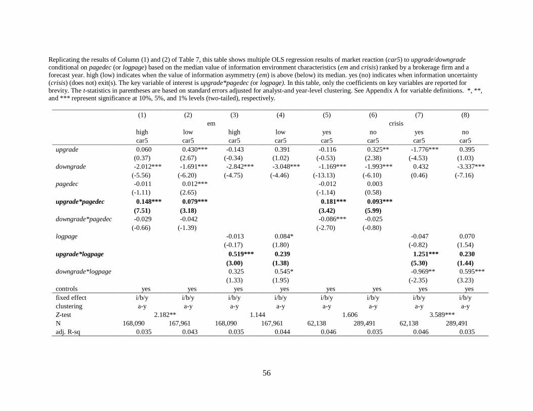
56

Replicating the results of Column (1) and (2) of Table 7, this table shows multiple OLS regression results of market reaction (car5) to upgrade/downgrade

conditional on pagedec (or logpage) based on the median value of information environment characteristics (em and crisis) ranked by a brokerage firm and a

forecast year. high (low) indicates when the value of information asymmetry (em) is above (below) its median. yes (no) indicates when information uncertainty

(crisis) (does not) exit(s). The key variable of interest is upgrade*pagedec (or logpage). In this table, only the coefficients on key variables are reported for

brevity. The t-statistics in parentheses are based on standard errors adjusted for analyst-and year-level clustering. See Appendix A for variable definitions. *, **, and *** represent significance at 10%, 5%, and 1% levels (two-tailed), respectively.

(1) (2) (3) (4) (5) (6) (7) (8)

em crisis

high low high low yes no yes no

car5 car5 car5 car5 car5 car5 car5 car5

upgrade 0.060 0.430*** -0.143 0.391 -0.116 0.325** -1.776*** 0.395

(0.37) (2.67) (-0.34) (1.02) (-0.53) (2.38) (-4.53) (1.03)

downgrade -2.012*** -1.691*** -2.842*** -3.048*** -1.169*** -1.993*** 0.432 -3.337***

(-5.56) (-6.20) (-4.75) (-4.46) (-13.13) (-6.10) (0.46) (-7.16)

pagedec -0.011 0.012*** -0.012 0.003

(-1.11) (2.65) (-1.14) (0.58)

upgrade*pagedec 0.148*** 0.079*** 0.181*** 0.093***

(7.51) (3.18) (3.42) (5.99)

downgrade*pagedec -0.029 -0.042 -0.086*** -0.025

(-0.66) (-1.39) (-2.70) (-0.80)

logpage -0.013 0.084* -0.047 0.070

(-0.17) (1.80) (-0.82) (1.54)

upgrade*logpage 0.519*** 0.239 1.251*** 0.230

(3.00) (1.38) (5.30) (1.44)

downgrade*logpage 0.325 0.545* -0.969** 0.595***

(1.33) (1.95) (-2.35) (3.23)

controls yes yes yes yes yes yes yes yes

fixed effect i/b/y i/b/y i/b/y i/b/y i/b/y i/b/y i/b/y i/b/y

clustering a-y a-y a-y a-y a-y a-y a-y a-y

Z-test 2.182** 1.144 1.606 3.589***

N 168,090 167,961 168,090 167,961 62,138 289,491 62,138 289,491

adj. R-sq 0.035 0.043 0.035 0.044 0.046 0.035 0.046 0.035

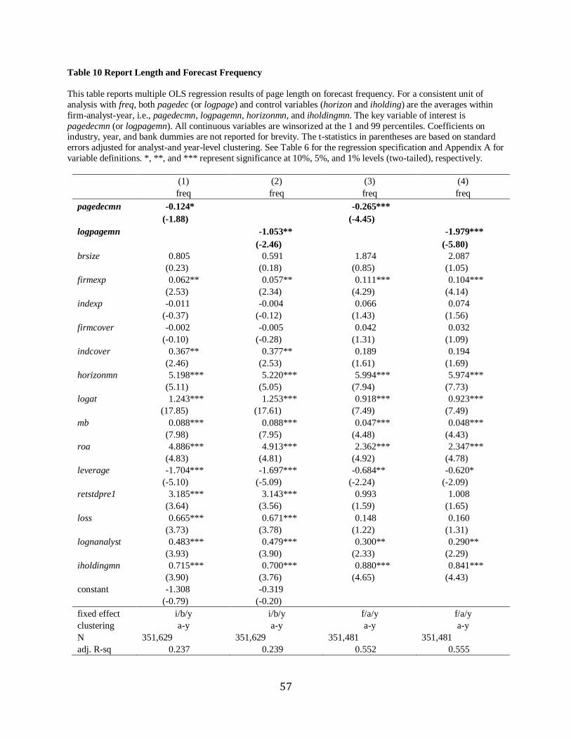
57

Table 10 Report Length and Forecast Frequency

This table reports multiple OLS regression results of page length on forecast frequency. For a consistent unit of

analysis with freq, both pagedec (or logpage) and control variables (horizon and iholding) are the averages within

firm-analyst-year, i.e., pagedecmn, logpagemn, horizonmn, and iholdingmn. The key variable of interest is

pagedecmn (or logpagemn). All continuous variables are winsorized at the 1 and 99 percentiles. Coefficients on industry, year, and bank dummies are not reported for brevity. The t-statistics in parentheses are based on standard

errors adjusted for analyst-and year-level clustering. See Table 6 for the regression specification and Appendix A for

variable definitions. *, **, and *** represent significance at 10%, 5%, and 1% levels (two-tailed), respectively.

(1) (2) (3) (4)

freq freq freq freq

pagedecmn -0.124* -0.265***

(-1.88) (-4.45)

logpagemn -1.053** -1.979***

(-2.46) (-5.80)

brsize 0.805 0.591 1.874 2.087

(0.23) (0.18) (0.85) (1.05)

firmexp 0.062** 0.057** 0.111*** 0.104***

(2.53) (2.34) (4.29) (4.14)

indexp -0.011 -0.004 0.066 0.074

(-0.37) (-0.12) (1.43) (1.56)

firmcover -0.002 -0.005 0.042 0.032

(-0.10) (-0.28) (1.31) (1.09)

indcover 0.367** 0.377** 0.189 0.194

(2.46) (2.53) (1.61) (1.69)

horizonmn 5.198*** 5.220*** 5.994*** 5.974***

(5.11) (5.05) (7.94) (7.73)

logat 1.243*** 1.253*** 0.918*** 0.923***

(17.85) (17.61) (7.49) (7.49)

mb 0.088*** 0.088*** 0.047*** 0.048***

(7.98) (7.95) (4.48) (4.43)

roa 4.886*** 4.913*** 2.362*** 2.347***

(4.83) (4.81) (4.92) (4.78)

leverage -1.704*** -1.697*** -0.684** -0.620*

(-5.10) (-5.09) (-2.24) (-2.09)

retstdpre1 3.185*** 3.143*** 0.993 1.008

(3.64) (3.56) (1.59) (1.65)

loss 0.665*** 0.671*** 0.148 0.160

(3.73) (3.78) (1.22) (1.31)

lognanalyst 0.483*** 0.479*** 0.300** 0.290**

(3.93) (3.90) (2.33) (2.29)

iholdingmn 0.715*** 0.700*** 0.880*** 0.841***

(3.90) (3.76) (4.65) (4.43)

constant -1.308 -0.319

(-0.79) (-0.20)

fixed effect i/b/y i/b/y f/a/y f/a/y

clustering a-y a-y a-y a-y

N 351,629 351,629 351,481 351,481

adj. R-sq 0.237 0.239 0.552 0.555

58

Impact of Environmental Disclosure in 10-K filings on Future Stock Price

Crash Risk: Textual Analysis

Abstract

Using textual analysis, the study examines the determinants of environmental disclosure (ED) in

U.S. 10-Ks and its impact on the future stock price crash risk. The level of (change in) ED is

positively (negatively) associated (autocorrelated) with litigation risk (one-year pre/post change).

Moreover, 10-Ks contain more negative ED than positive one. Accordingly, the research finds

the negative association of ED with short term returns, showing that ED is bad news for

managers to hide. In the long term, increased ED results in decreased risk in significant stock

price drop. Change and instrument variable analyses mitigate endogeneity and identify a

potential causation. The results are consistent with the notion that firms benefit from non-

financial information disclosure.

Keywords: Environmental disclosure; Stock price crash risk; Managers’ bad news hoarding

tendency; 10-Ks; Textual analysis

59

1. Introduction

SEC Regulation S-K and accounting standards relating to contingencies (SFAS No. 5)

mandate a firm to disclose a probable and reasonably estimated environmental expenditure in

financial statements in 10-Ks. Due to the limitations of accounting rules, however, a firm may

discretionarily disclose supplementary environmental information in 10-Ks. The study expands

the literature on the value relevance of environmental disclosure by examining the impact of

environmental disclosure in 10-Ks on future stock price crash risk based on managers’ bad news

hoarding tendency.

Due to information asymmetry and agency problem, opportunistic management tends to

hoard bad news than good news until a tipping point when a large amount of bad news is

abruptly released, leading to a sudden drop in stock price or a crash (Jin and Myers, 2006).

Accordingly, disclosing the negative nature of environmental information mitigates managers’

bad news hoarding incentive, resulting in less crash risk.

Based on textual analysis of 81,826 10-Ks filed to Securities and Exchange Commission

(SEC) by U.S. firms during 1998-2013, the research first identities disclosed environmental

information as bad news by documenting its positive relationship of environmental disclosure

with litigation risk which is another bad news. The study also finds evidence of disclosed

environmental information as bad news by showing that environmental disclosure is mean

reverting since bad news is more likely to be concealed relative to good news. Additionally, the

research provides direct evidence by finding that negative environmental information is

disclosed more than positive environmental information by 1.2%. Meanwhile, if this is the case,

the stock market should negatively react to environmental disclosure around a 10-K filing date.

The research confirms this by documenting a significantly negative association of environmental

60

disclosure with cumulative abnormal returns two days before and after the filing date. Thus, the

study shows that disclosed environmental information in 10-Ks is bad news, thereby allowing for

the examination of whether environmental disclosure reduces future crash risk based on the

hypothesis that managers tend to hoard bad news.

The paper provides empirical evidence that a firm with more environmental disclosure is

less likely to experience major price drops in the future because of a lower tendency on the part

of managers to hoard bad news. The logit regression shows that a one standard deviation increase

of environmental disclosure reduces the odds of future crash risk by 10%, holding everything

else constant. On the other hand, the findings are robust to different measures of environmental

disclosure such as its change, dummy, and residual. Using two exogenous shocks as an

instrumental variable, the research further identifies a potential causality, over and above

mitigating potential endogeneity issues. Overall, the results are consistent with the idea that firms

benefit from non-financial information disclosure (e.g., Amir and Lev, 1996).

The research also examines the determinants of environmental disclosure, and finds its

positive (negative) association with current return, firm size, leverage, litigation risk, the

membership of environment-sensitive industry, and 10-K file size (previous return volatility, and

turnover). More importantly, Neu, Warsame, and Pedwell (1998) find the complementary role of

other social disclosures to environmental disclosure in 10-Ks because they help to frame the

interpretation of environmental disclosure. Motivated by this, the paper documents that disclosed

environmental information is positively (negatively) associated with human rights (product

responsibilities).

The study makes the following important contributions. First, the paper adds to a growing

literature on non-financial disclosure and its economic consequences by showing that

61

environmental disclosure predicts future crash risk. Prior studies on environmental disclosure

focus on its impact on return performance. However, the study establishes a potential causal

relationship between environmental disclosure and ex-post crash risk using two exogenous

shocks as an instrumental variable.

The study also contributes to the literature on stock price crash risk by comparing two

different proxies for crash risk, i.e., one from finance and another from accounting literature.

Previous crash risk studies (e.g., Hutton, Marcus, and Tehranian, 2009) measure crash risk based

on firm-specific weekly abnormal returns that is net of market and industry influences. Contrary

to this prior research, following Savor (2012), the paper introduces another crash risk measure

considering the effect of a market, size, and value factor. This addition broadens the

understanding of the impact of environmental disclosure on firms and stakeholders.

The research contributes to the literature using textual analysis by showing its usefulness

to identify an underlying theory of managers’ bad news hoarding. On the other hand, to my

knowledge, the sample of 81,826 firm-year observations from mandatory 10-K filings during

1998 to 2013 is by far the largest among textual analysis on either environmental disclosure or

crash risk. A large sample size allows the study to examine and generalize the economic

consequences of environmental disclosure and especially, its causality using exogenous shocks.

Previous textual analyses on environmental disclosure or crash risk have less sample size. For

example, Ertugrul, Lei, Qiu, and Wan (2017) with 32,207 10-Ks for annual report readability-

crash risk test, Cho and Patten (2007) with 100 10-Ks for environmental disclosure-

environmental performance test during 2002, Neu, Warsame and Pedwell (1998) with 330 10-Ks

from 33 Canadian firms for environmental disclosure-external pressure test, and Patten (1992)

with 131 10-Ks for environmental disclosure-Alaskan oil spill test.

62

This paper proceeds as follows. Section 2 reviews the relevant literature and develops the

hypotheses. Section 3 explains the research design and the sample collection. Section 4 presents

the main empirical analysis. Section 5 describes the robustness checks. Section 6 discusses the

identify strategies. Section 7 concludes the paper.

2. Literature review and Hypothesis development

In this section, the study reviews literature on the consequences of mandatory and/or

voluntary environmental disclosure since its main investigation is on the stock price crash risk

impact of environmental disclosure explained by managers’ had news hoarding tendency. Based

on the explanation, two hypotheses are developed.

2.1 Literature on consequences of environment disclosure

Under SEC regulations (e.g., Regulation S-K) as well as accounting standards on

contingencies (SFAS No. 5), a firm must disclose a probable and reasonably estimated

environmental expenditure in financial statements in 10-Ks.17 The rules on environmental

disclosures in 10-Ks include items 101/103/104/303 from Securities Act of 1933 and Securities

Exchange Act of 1934 and Staff Accounting Bulletin No. 92. Appendix 1 briefly discusses these

SEC rules on environment disclosure.

Different from mandatory environmental disclosure, voluntary environmental disclosure

is not required by the SEC. Grossman (1981) and Milgrom (1981) argue that a firm should

voluntarily disclose all relevant information to prevent an unjustified undervaluation due to

information asymmetry. In contrast, there is a lack of full voluntary environmental disclosure

based on legitimacy theory (e.g., Gray, Kouhy and Lavers, 1995b; Deegan, 2002: Patten, 1992;

17 With regard to the measurement of a contingent loss, FASB Interpretation No. 14, Reasonable Estimation of the

Amount of a Loss, states that the minimum be accrued when the reasonable estimate of a loss is a range but no

amount within the range is a better estimate than any other amount.

63

Neu, Warsame and Pedwell, 1998), information asymmetry from agency theory (e.g., Li,

Richardson and Thornton, 1997), and economics-based theory (e.g., Li, Richardson and

Thornton, 1997). In sum, the level of voluntary environmental disclosure changes depending on

the environmental information demand from stakeholders or on the motivations on the

environmental information supply from managers.

Previous studies on the economic impact of environmental disclosure fall largely into

three streams depending on its types (i.e., mandatory or voluntary) and consequences. The first

stream examines the value relevance of disclosed environmental information under SEC-

mandated environmental disclosure requirements (Blacconiere and Patten, 1994; Blacconiere and

Northcut, 1997; Al-Tuwaijri, Christensen, and Hughes, 2004). The consensus is that more

mandatory environmental disclosure is positively related to firm value, suggesting that

mandatory disclosure reduce information asymmetry between managers and investors (Lev,

1988). In other words, investors interpret environmental disclosure as a positive sign for firms to

manage their exposures to future regulatory costs, which thus positively influences a firm’s

value.

Compared to the studies on the effect of the mandatory environmental disclosure, the

second stream of literature examines stock market reactions to voluntary environmental

disclosure. The findings remain inconclusive due to the heterogeneous nature of the information

discretionarily disclosed. For instance, Belkaoui (1976) shows positive abnormal stock returns

for voluntary announcements of expenditure on pollution control in the annual report. However,

Ingram (1978) reports no stock performance impact of voluntary social responsibility disclosures

regarding the environment, fair business, personnel, community, and product in the annual

reports of Fortune 500 companies.

64

The third steam examines the impact of environmental disclosure on the cost of capital.

Richardson and Welker (2001) find that voluntary social disclosure including environmental

disclosure in Canadian annual reports increases the cost of equity capital, especially for more

profitable firms.18 Their findings are opposite to the notion that discretionary disclosure reduces

information asymmetry.

Thus, another economic impact of environmental disclosure, i.e., stock price crash risk,

has not been explored for a long period of time.

2.2 Hypothesis development: environmental disclosure and crash risk

The study expands the literature on the value relevance of environmental disclosure by

exploring the effect of environmental disclosure in 10-Ks on stock price crash risk. The

underlying theory to explain its impact on crash risk is managers’ bad news hoarding tendency.

Pae (2005) argues that a firm with information advantage tends to hoard bad news than

good news, resulting in an increase in investor uncertainty. Considering this, Jin and Myers

(2006) conjecture that when management cannot hoard bad news up to some tipping point, a

large amount of bad news is abruptly and immediately released to the stock market, leading to a

sudden drop in stock price, i.e., a crash. They contend that the probability and magnitude of a

future stock price crash risk increases with the opacity of financial reporting which incentivizes a

manager to withhold bad news from public disclosure.

The economics-based theory also supports the manager’s bad news hoarding tendency

which depends on the cost-benefit outcome of disclosure (Chambers and Penman, 1984; Kross

and Schroeder, 1984), and career concerns and management compensation structure (Nagar,

1999; Nagar, Nanda, and Wysocki, 2003; Kothari, Shu, and Wysocki, 2009). However, litigation

18 One explanation for this is that a firm discloses more social information to promote itself. That is, it overreports

its positive contributions, but underreports negative social effects.

65

risk and reputation concerns motivate managers to quickly reveal bad news (Kasznik and Lev,

1995; Skinner, 1994, 1997). Accordingly, future stock price crash risk has a positive association

with discretionary accruals (Hutton, Marcus and Tehranian, 2009), complex tax planning (Kim,

Li, and Zhang, 2011a, 2011b), and an executive compensation package (Benmelech, Kandel, and

Veronesi. 2010; Kim, Li, and Zhang, 2011b), but a negative relationship with the adoption of

International Financial Reporting Standards (DeFond, Hung, Li, and Li, 2015), accounting

conservatism (Kim and Zhang, 2015), and earnings smoothing (Chen, Kim, and Yao, 2015).

Using a CSR performance score from the MSCI ESG database, Kim, Li, and Li (2014)

find that a firm with a better score has a lower crash risk. Following them, previous research has

mixed results. Lu and Nakajima (2014) show that CSR has no effect on reducing the stock price

crash risk of Japanese firms. Contrary, Lee and Lee (2016) show that CSR significantly mitigates

Taiwanese stock price crash risk. Similarly, Zhang, Xie, and Xu (2016) document the negative

impact of corporate philanthropic action on crash risk in China.

Methodologically, Kim, Li, and Li (2014) use a CSR performance index from the MSCI

ESG database which scores the existence of disclosure items from firms’ annual reports and CSR

reports. However, the study focuses on the annual report filed by publicly traded firms pursuant

to the Securities Exchange Act of 1934 in Form 10-K which is the primary source of information

for capital market participants such as shareholders, creditors, and financial analysts.

To investigate the effect of environmental disclosure on future crash risk, it is critical to

show that environmental disclosure is bad news that management tends to keep inside the firm

for an extended period. Using SEC-registered mine owners, Christensen, Floyd, Liu, and Maffett

(2017) document a negative short-window market reaction around the disclosure of immediate

danger orders (IDOs) through a Form 8K filing required by 2010 Dodd-Frank Act, suggesting

66

that IDOs are bad news which investors react negatively. They argue that the inclusion of

information on social responsibility (i.e., safety at work) in financial reports can have a real

effect.

As a major component of CSR, it is worth to investigate the economic consequence of

environmental disclosure in 10-Ks. Thus, the study hypothesizes that more environmental

information in 10-Ks reduces information asymmetry for external investors, which mitigates a

manager’s bad news hoarding incentive, leading to less crash risk than a firm with less voluntary

environmental disclosure. In sum, the research predicts that firms with more environmental

disclosure in 10-Ks are less likely to experience major price drops in the future due to less bad

news hoarding from management.

Hypothesis 1: Environmental information disclosed in 10-K filings is negatively related with

short-term market reaction.

Hypothesis 2: Environmental information disclosed in 10-K filings is negatively related with

future stock price crash risk.

3. Research methodology and sample

3.1 Measurement of environmental disclosure in 10-K filings

Studies on environmental disclosure focus on the quantity (e.g., Neu, Warsame and

Pedwell, 1998; Patten, 1992), the thematic content (e.g., Hughes, Anderson, and Golden, 2001),

and the tone (Cho, Roberts, and Patten, 2010). This reflects the intense debate on the most

appropriate unit of analysis for textual analysis (Gray, Kouhy and Lavers, 1995b). Nevertheless,

most studies on social and environmental disclosure tend to use one or a combination of words,

sentences, and pages (Hackston and Milne, 1996). Following this, the study uses a dictionary

(i.e., a collection of keywords) approach to extract every environment-related sentence. The

67

research creates a dictionary that is tailored to environmental disclosure in 10-K filings based on

the following procedures.

1) I download 10-Ks from SEC's Electronic Data Gathering, Analysis, and Retrieval (EDGAR)

database. I randomly select twenty-two 10-Ks and read each of them to manually extract a

word and phrase that is related to environmental information.

2) Since environmental activity is an integral part of CSR dimensions, I also search the

keywords in the CSR-related websites such as Global Reporting Initiative (GRI) and MSCI

ESG indexes.

3) I combine all the keywords from Step 1 and 2 to generate the preliminary dictionary of

environmental disclosure. Using a Java program, I identify every sentence from a 10-K filing

that contains any of the keywords in the dictionary.

4) I manually verify each and every keyword by reading more than twenty randomly-selected

sentences that include the keyword.

Appendix 2 reports the top fifty most frequent environment-related keywords in 10-Ks.

Appendix 3 shows examples of sentences on environmental disclosure. To measure the overall

level of environmental disclosure in 10-Ks, I count the total number of environment-related

keywords in each 10-K filing.

For a change analysis, I compute the change in the total number of environment-related

keywords from year t-1 to year t, scaled by the average number of environment-related keywords

in the 10-K filings for the years, i.e., ∆envt=(∆envt-∆envt-1)/(∆envt+∆envt-1).

For more robustness checks, I also create two alternative measures of environmental

disclosure: 1) a dummy variable of environmental disclosure equal to one if the number of

environment-related keywords in a 10-K filing is above its median, and zero otherwise in year t,

68

and 2) a continuous variable of abnormal environmental disclosure equal to residuals from

regressing environmental disclosure on explanatory variables in year t. See Appendix 4 for

variable definitions.

3.2 Measurement of short-term market reaction

To test the short-term market reaction to environmental disclosure, the dependent

variable, cumulative abnormal return (car5), is measured as the sum of daily market-adjusted

abnormal return during five ([-2, +2]) days starting from two days before a 10-K filing date as

day 0.

car5i,t= exp[∑ 𝑙𝑛(1 + 𝑟𝑒𝑡𝑢𝑟𝑛𝑖, 𝑡 − 𝑣𝑤𝑟𝑒𝑡𝑑𝑖, 𝑡)] − 12𝑡=−2 (1)

where returni,t is the daily stock return, and vwretdi,t is the value-weighted market return on stock

i in time t. Specifically, 10-K filing dates are captured from a 10-K per se downloaded from

SEC's EDGAR database. The daily stock return is based on the holding period return from

CRSP, and the market return is the daily value-weighted return including all distributions of U.S.

stocks from CRSP. Appendix 4 provides variable definitions.

3.3 Measurement of crash risk

The study uses two different proxies for crash risk depending on reflecting significant

changes in fundamentals or investor sentiment. The first and main crash risk measure (shockff3)

follows the spirit of Savor (2012). Savor (2012) defines major price movements as any firm-date

observation where the absolute value of the Fama-French three-factor plus momentum model-

adjusted abnormal return exceeds 10%.19 He argues that 10% threshold is “high enough to screen

out most price movements that do not reflect either substantial changes in fundamentals (or

19 Savor (2012) finds that the results hold even if returns are scaled by their lagged volatility.

69

market perception thereof) or in investor sentiment”. Atkins and Dyl (1990) and Bremer and

Sweeney (1991) also use the 10% thresholds to define large price declines.

Following them, firm-specific weekly abnormal return is measured as the residual return

from the Fama-French three-factor model below that is net of market, firm size and firm value

influences.

Ri,𝑡--Rf,=𝛼𝑖+𝛽i,m(R𝑚,𝑡-Rf,𝑡)+𝛽i,smbSMBt+𝛽i,hmlHMLt+𝜀i,𝑖, (2)

where Ri, is the firm’s return, Rm, is the market return (i.e., CRSP value-weighted), Rf,𝑡 is the

risk-free rate, SMBt is the return difference between a portfolio of small and big stocks (size

factor), and HMLt is the return difference between a portfolio of high and low book-to-market

stocks in week t (value factor). Then, following Savor (2012), Atkins and Dyl (1990), and

Bremer and Sweeney (1991), a major price drop, shockff3, is an indicator equal to one if weekly

firm-specific abnormal return (𝜀i,𝑖) is less than -25% within one year post the release of 10-K

filings. Even though -25% threshold is arbitrary, it is well below than -10% to secure an extreme

price drop. The results are robust to various cutoffs, both higher and lower, and to different

measures of returns such as raw returns, market- or industry-adjusted returns, or market-model

excess returns.

Compared to shockff3 which is still influenced by an industry factor, the second and

alternative crash risk measure (crash) is based on the firm-specific weekly abnormal return that

is net of market and industry influences (Hutton, Marcus, and Tehranian, 2009). Specifically, I

define the firm-specific weekly return, denoted by W, as the natural logarithm of one plus the

residual return from the industry-adjusted expanded market model regression below.

𝑟j,𝑡=𝛼𝑖+𝛽1j𝑟𝑚,𝑡−1+𝛽2j𝑟ind,𝑡−1+𝛽3j𝑟𝑚,𝑡+𝛽4j𝑟ind,𝑡+𝛽5j𝑟𝑚,𝑡+1+𝛽6j𝑟ind,𝑡+1+𝜀j,𝑖, (3)

70

where rj,t is the return on stock j in week t, rm,t is the return on the CRSP value-weighted market

index in week t, and rind,t is the industry return based on Fama-French 49 industry classification. I

include the lead and lag terms for the market and industry returns to allow for nonsynchronous

trading. The firm-specific weekly return for firm j in week t, Wj,t, is measured as ln(1+ 𝜀j,t) from

Equation (3). crash is defined as the occurrence of any week with the firm-specific return (Wj,t)

exceeding 3.09 standard deviations below its mean value within one year post the release of 10-

K filings. The choice of 3.09 is meant to generate a frequency of 0.1% in the normal distribution.

See Appendix 4 for variable definitions.

In sum, a major difference between two firm-specific abnormal returns, i.e., shockff3 and

crash is that the first is influenced by an industry factor, whereas the latter is influenced by a size

and value factor.

3.4 Regression specification

To examine whether environmental information disclosed in 10-Ks is bad news, I regress

the measure of short-term market reaction on environmental disclosure as follows.

car5i,t=β0 + β1envi,t + ∑ 𝛽𝑚𝑀𝑚=2 Xi,t + µ j + ŋt + εt (4)

where i stands for firm, j for industry, and t for time. The vector of control variables is denoted

by Xi,t, which includes return (ret), return volatility (stdret), trading volume (turnover), size

(logat), growth (mb), profitability (roe), leverage (leverage), proportion of institutional investors’

holding (iholding), rate of litigation-related words (litigious), membership of environmental-

sensitive industry (esi), other CSR-dimensions (hrtotwords, retotwords, and sototwords), and

total number of words in a 10-K (totwords). Following crash risk literature, Xi,t also includes the

negative of the third moment of firm-specific weekly returns (ncskewlag), and earnings

management level (em). The control variables are explained below in detail since the crash risk

71

effect of environmental disclosure is the main research question. 𝛽1 in the regression is the

coefficient of interest, which measures the impact of env on car5.

For the impact of environmental disclosure on crash risk, I regress a dependent variable

of crash risk on a measure of environmental disclosure. I add the event return, car5, to control

variables from the market reaction model above that might affect a firm’s downside risk. The

baseline regression model is as follows,

dependenti,t+1=β0 + β1∑ 𝛽𝑚𝑀𝑚=2 indepi,t + ∑ 𝛽𝑛

𝑁𝑛=𝑚+1 Xi,t + µ j + ŋt + εt (5)

where the dependent variable (dependent) is one of the proxies for crash risk (i.e., shockff3 and

crash) measured in year t+1. The key variable of interest (indep) is one of the proxies for

environmental disclosure (i.e., env, ∆env, envdum, and envres). The rest of variables control for

factors which influence dependent variables.

All the regressions include industry dummies denoted as µ j and year dummies denoted as

ŋt to control for unobserved time-invariant industry and year factors. Industry indicator variables

are based on the 24 Global Industry Classification Standard (GICS) codes. In addition, standard

errors are adjusted for clustering at the firm (state for the second identification strategy) and year

level to control for potential bias in the estimates when the residuals of a firm are correlated

across firms and years.

As for the control variables, I follow the previous literature to control for a set of factors

that predict future stock price crash risk. Chen, Hong, and Stein (2001) find that firm size, past

returns, and stock turnover predict crash risk. Hence, I control for firm size (logat) in year t,

returns (ret), and trading volume (turnover). Similarly, I include both announcement returns

(car5) around 10-K filings with a five-day window [-2, 2]. They also contend that more volatile

72

stocks are more prone to a future stock price crash. Therefore, I control for stock return volatility

(stdret and ncskewlag).

Hutton, Marcus, and Tehranian (2009) find that glamour stocks with a high market-to-

book ratio (mb) have higher crash risk due to a bubble buildup in the past. Thus, I control for mb.

They also document that crash risk is negatively related to operating performance and financial

leverage but positively associated with earnings management. Accordingly, I control for

profitability (roe), financial leverage (leverage), and earnings management (em).

Andreou, Antoniou, Horton, and Louca (2016) find that effective corporate governance

mechanisms are associated with lower firm-specific stock price crashes since they help to reduce

opportunistic managerial behavior. Thus, I control for the proportion of institutional investors’

holding (iholding).

Kasznik and Lev (1995) and Skinner (1994, 1997) show that litigation risk motivates

managers to quickly reveal bad news, suggesting their less bad news hoarding tendency leading

to less crash risk. Therefore, I control for the level of litigation risk (litigious) using the

proportion of litigation-related words relative to the total words in a 10-K.

Following Cho and Patten (2007) who document that firms in the environment-sensitive

industry (esi) tend to provide more environmental disclosure, I control for the membership of esi.

Neu, Warsame and Pedwell (1998) argue the complementary role of other social

disclosures to environmental disclosure in 10-Ks because they help to frame the interpretation of

environmental disclosure. Accordingly, I additionally control for the other dimensions of

corporate social responsibility (CSR) disclosures on human rights (hrtotwords), product

responsibilities (retotwords), and society (sototwords) which influence the level of

environmental disclosure.

73

I also control for qualitative factors on the crash risk using the number of total words in a

10-K (totwords). All the independent variables are measured in year t while the dependent

variables are measured in year t+1. All continuous variables are winsorized at 1 and 99

percentiles to reduce the effect of outliers. Appendix 4 provides variable definitions.

3.5 Sample construction

I download all 10-Ks from the SEC's Electronic Data Gathering, Analysis, and Retrieval

(EDGAR) database filed from January 1998 through March 2013. Based on Campbell, Chen,

Dhaliwal, Lu, and Steele (2014), I construct the sample as follows:

1) I exclude 10-Ks with less than 1,000 words, and late fillings such as NT 10-K, NT 10-KA,

and NTN 10-K under Rule 12b25 of inability to timely file all or part of the 10Ks.

2) EDGAR identifies firms that file 10-Ks using Central Index Key (CIK). To match CIK and

filing dates from 10-Ks with PERMNO and filing dates from the CRSP-COMPUSTAT

merged data, I use the Wharton Research Data Services (WRDS) CIK-PERMNO file. I

exclude all firms for which I am not able to match CIK to GVKEYs and the filing dates.

3) I exclude all firms without relevant fundamentals and stock market data from COMPUSTAT

and CRSP. I also exclude all firms which have data less than 15 weeks per year.

4) I limit returns between -1 and 2. The final sample contains 81,826 firm-year observations and

9,799 unique firms between January 1998 and March 2013.

4. Empirical results

4.1 Descriptive statistics

Table 1, Panel A, reports the descriptive statistics for the main variables. In the sample,

the mean values of shockff3 and crash are 0.201 and 0.295, respectively. This suggests that the

unconditional probabilities of a firm’s stock price crash risk over a year are around 20% to 30%

74

similar with previous crash risk literature. Meanwhile, disclosed environmental information

accounts for 0.08% of the total information in the annual report, whereas litigation-related

information for 1.2%. 14% of the sample belongs to the industries sensitive to environment.

Panel B of Table 1 shows the distribution of the sample by year between 1998 and 2013.

The mean number of a firm’s 10-K filings gradually decreases. The mean value of environmental

disclosure decreases until 2005, and then increases to the highest level of 0.1% in 2013.

Specifically, its increase never stops after the legal standing of emissions and climate change in

Massachusetts v. U.S. Environmental Protection Agency (EPA) in 2007. Moreover, the largest

increase is recorded in 2010 when BP’s Deepwater Horizon drilling rig is exploded in the Gulf of

Mexico in April 2010. Thus, the year distribution provides two exogenous shocks to mitigate

endogeneity and further identify a potential causality.

The mean values of shockff3 reach to the highest points during the pinnacles of market

crashes in 2001 and 2008. The mean values of crash have a similar trend with shockff3. Figure 1

graphically shows the negative association between environmental disclosure (env) and crash

risk (shockff3), providing initial evidence that the more environmental disclosure, the less future

crash risk.

Panel C of Table 1 summarizes the sample distribution by 24 industry groups based on

the Global Industry Classification Standard (GICS) codes. Similar with Figure 1, Figure 2

graphically displays the negative relationship between environmental disclosure (env) and crash

risk (shockff3). Specifically, utilities, materials, and energy are the top three industries in terms

of environmental disclosure. On average, they account for 0.3%, 0.27%, and 0.23% of env,

respectively, which is about three times higher than 0.09% of its mean value. They tend to have

less mean values of crash risk proxies compared to industries with less environmental disclosure.

75

This implies that if a firm belongs to an industry with more environmental disclosure, it is less

likely to experience stock price crash in the future.

Meanwhile, utilities have the highest environmental disclosure, whereas banks have the

lowest with the least crash risk. This suggests that they are regulated and even protected by

government, and provides the rationale for a robustness test after excluding them from the

sample.

Panel D of Table 1 displays the Pearson correlation matrix of the main variables. As

expected, two measures of crash risk are positively correlated with 0.351 of coefficient,

suggesting that these measures capture the overlapping but different aspects of the skewness in

return distributions, i.e., crash. As expected, the level measure of environment disclosure (env) is

significantly and negatively correlated to all crash risk measures, suggesting that high

environment disclosure firms are less likely to experience sudden stock price drop in the future.

4.2 Univariate test

Table 2 shows the mean comparisons of crash measures (shockff3 and crash) based on

the median value of environmental disclosure, envdum equal to one if env is above its median,

and zero otherwise.

As envdum increases, shockff3 significantly decreases, whereas crash is not significant.

As in the descriptive statistics in Table 1, this provides additional initial evidence that the greater

environmental disclosure, the less crash risk in the future.

4.3 Determinants of environmental disclosure

To identify the determinants of environmental disclosure, I regress env on the same

explanatory variables from Equation (4) after replacing stdret with stdretpre12 and excluding

ncskewlag and em. The regression model is as follows,

76

envi,t=β0 + ∑ 𝛽𝑚𝑀𝑚=1 Xi,t + µ j + ŋt + εt (6)

where i stands for firm and t for time. The vector of control variables is denoted by Xi,t, which

includes return (ret), previous return volatility (stdretpre12), trading volume (turnover), size

(logat), growth (mb), profitability (roe), leverage (leverage), proportion of institutional investors’

holding (iholding), proportion of litigation-related words (litigious), membership of

environmental-sensitive industry (esi), other CSR-dimensions (hrtotwords, retotwords, and

sototwords), and total number of words in a 10-K (totwords). The model includes industry fixed

effect to account for cross-industry differences and year fixed effect to control for common time

trends. Standard errors are cluster-adjusted at firm and by year levels. All continuous variables

are winsorized at 1 and 99 percentiles to reduce the effect of outliers. Appendix 4 provides

variable definitions.

Table 3 reports OLS regression results on the determinants of environmental disclosure.

Consistent with previous literature (e.g., Neu, Warsame and Pedwell, 1998), environmental

disclosure is positively associated with firm size (logat) and the membership of environment-

sensitive industry (esi). Previous literature documents the mixed results on its relationship with

profitability (roe) and leverage (leverage). The results show its positive correlation with

leverage, ret, hrtotwords, and totwords, while its negative association with stdretpre12, turnover,

and retotwords. Particularly, its positive correlation with litigious suggests that environmental

disclosure is closely related to litigation risk of which tone is mostly negative, implying that it is

bad news which managers tend to hide.

4.4 Evidence of Environmental Disclosure as Bad News

To test the hypotheses, it is crucial to show that environment information disclosed in 10-

Ks is bad news since the link between environmental disclosure and crash risk is explained only

77

by managers’ bad news hoarding tendency. Specifically, if environmental information is bad

news, then managers tend to hide it for an extended period until it is abruptly revealed to the

public, leading to a significant drop in stock price. In other words, their lower tendency of bad

news hoarding is highly likely to reduce the future crash risk. Thus, to show that disclosed

environmental information is bad news, the study implements a battery of tests.

First, the research shows the positive relationship of environmental disclosure with

litigation risk of which tone is mostly negative, providing evidence that the former is bad news

related to litigation. Panel A of Table 4 reports confirms this by showing the positive association

between environmental disclosure (env) and litigation risk (litigious). Panel B of Table 4 presents

the results of the univariate test on mean comparisons of environmental disclosure measure (env)

based on the median value of litigious (litigiousdum). litigiousdum is equal to one if litigious is

above its median, and zero otherwise. The results show that as litigious increases, env also

significantly increases. As described in Section 4.3, Table 3 reports the positive association

between env and litigious after controlling for various variables. The results suggest that

disclosed environmental information is litigious-related and thus, negative news for a firm to

hide.

Compared to good news relatively quickly disclosed by managers, bad news tends to be

concealed. Accordingly, less disclosure of bad news will revert to the mean, i.e., mean reverting

by more disclosure of it in the future. In other words, if disclosed environmental information is

bad news, then it will be mean reverting. Panel C of Table 4 shows the results of the mean

reversal of the change values in environmental disclosure. ∆envlag (∆envlead) is the difference

between ∆env and previous (next)-period ∆env. ∆env is negatively associated with both ∆envlag

78

and ∆envlead, supporting its mean reversal. This suggests that disclosed environmental

information is bad news.

Panel D of Table 4 provides direct evidence that disclosed environmental information is

bad news by comparing the relative proportion of the number of negative (envneg) and positive

(envpos) environment-related keywords to the number of total environmental-related keywords

when the number of total environmental-related words is greater than 0 in a 10-K filing in year t.

The summary statistics show that the negative environmental information is more disclosed than

the positive one by 1.2%, i.e., 3.4% vs. 2.2%.

Overall, the results suggest that disclosed environmental information is bad news,

supporting managers’ bad news hoarding tendency related to future crash risk.

4.5 Environment disclosure and short-term market reaction

Market negatively reacts to bad news. As shown in Section 4.4, if disclosed

environmental information is bad news, then investors show a negative reaction to it. Consistent

with this, the results of Table 5 display the significantly negative association between env and

car5 at p<0.05 after controlling for various factors across models. Thus, the results confirm the

first hypothesis. car5 is cumulative abnormal returns above value-weighted market returns for 5

trading days around a 10-K filing date (i.e., -2 to +2 with day 0 as the filing date).

4.6 Environment disclosure and crash risk

Table 6 reports the logit regression results of the impact of environmental disclosure on

crash risk. In Columns (1) to (2), the dependent variable is shockff3 which is an indicator equal

to one if there is any week during which the abnormal return based on Fama-French three-factor

is less than -25% within one year post the release of a 10-K filing, and zero otherwise. In

Columns (3) to (4), the dependent variable, crash, is an indicator equal to one if a firm

79

experiences any firm-specific weekly returns exceeding 3.09 standard deviations below the mean

firm-specific weekly return within one year post the release of a 10-K filing, and zero otherwise.

Across all models of Table 6, I find that env, which is measured as the ratio of the total

number of environment-related keywords to the total number of words in 10-Ks, is negative and

statistically significantly related to both measures of crash risk (shockff3 and crash). Untabulated

tables show that the results are robust to the model after excluding an industry fixed effect to

avoid capturing the industry effect twice due to esi, or vice versa, whose significance is stronger

in general.

Overall, the study provides empirical evidence that more environmental disclosure in 10-

Ks is associated with lower future stock price crash risk. The results are consistent with the

second hypothesis, suggesting that even small proportion of environmental disclosure with

average 0.08%.of 10K’s total disclosure) is highly likely to make a significant impact on future

crash risk.

To assess the economic significance of environmental disclosure, I compute the odds

ratios for model (2) and (4) of Table 6 using the standard deviation reported in Panel A of Table

1. The odds ratios for a one standard deviation increase in env are 0.95 and 0.97 for each model,

indicating that a one standard deviation increase in env reduces the odds of future crash risk

(shockff3 and crash) by 10% if I fix all the other variables at a fixed value. In comparison, a one

standard deviation increase in firm size (logat) reduces the odds of shockff3 and crash by 7% and

8%, respectively. The results suggest that the negative association between environmental

disclosure and future stock price crash risk is economically significant.

Table 6 also shows that when the dependent variable is shockff3 in Columns (1) and (2),

crash risk is negatively correlated with cumulative abnormal return around the 10-K filing

80

release date (car5), current return (ret), firm size (at), profitability (roe), and corporate

governance (iholding), but positively related with stock return volatility (stdret and ncskewlag),

information asymmetry level (turnover), financial performance (leverage), the total number of

words in a 10-K filing (totwords), and the level of earnings management (em). When the

dependent variable is crash in Columns (3) and (4), the coefficients on the control variables

largely have a similar statistical significance with those of shockff3.

Meanwhile, Loughran and McDonald (2014) find that a 10-K filing with a larger size is

associated with higher volatility within one month after the filing due to its complexity.

Motivated by this, Li and Zhao (2016) reveal another role of 10-K disclosures, i.e., an

information role (or transparency), and document that a larger 10-K filing in two months

following the filing is associated with a bigger reduction in volatility. 20 In Table 6, however, the

positive association between crash risk measures (shockff3 and crash) and a file size proxy

(totwords) supports more information asymmetry due to the complexity of 10-Ks in a longer

term, i.e., up to one year after the filing, inconsistent with the findings of Li and Zhao (2016).

5. Robustness checks

In this section, I implement a battery of robustness tests on the results of Column (2) and

(4) Table 6, and show that the results are robust to various tests. In an odd number Columns, the

dependent variable is shockff3, while in an even number Columns, the dependent variable is

crash.

5.1 Change, dummy, and residual variable of environmental disclosure

20 Previous literature (e.g., Li, 2008) uses the number of 10‐K words as a measure of complexity. Loughran and

McDonald (2014) find that a 10-K file size is positively correlated with the number of 10‐K words (0.712 of

correlation coefficient).

81

The panel data allows us to do time-series tests to explore a directional effect and to

eliminate a time-invariant effect. However, reverse causality due to self-selection may be a

concern for the empirical findings. The reason is that firms with more crash likelihood are more

likely to disclose environment information in 10-Ks filings. To address this endogeneity issue, I

first conduct a change analysis. Specifically, I examine whether changes in environmental

disclosure in 10-Ks are negatively associated with future stock price crash risk.

Column (1) and (2) of Panel A of Table 7 show that the change in environment disclosure

(∆env) in 10-Ks is significantly negatively related to future crash risk, consistent with the

findings for the level of environmental disclosure in Table 6.

Next, I divide the sample into two groups based on a median value of env, and create a

dummy variable, envdum, when the group with a higher value of env takes one, and zero for a

lower value relative to the median of env. The results of Column (3) and (4) of Panel A of Table

7 are consistent with the hypothesis that more environmental disclosure results in a lower

probability of stock price crash risk in the future.

Lastly, to deal with endogeneity issue that both environmental disclosure and crash risk

are determined by some common uncontrolled factors, I adopt a two-stage regression approach

to first estimate residual environmental disclosure (envres) by replicating Column (2) of Table 3,

and then use envres to predict future crash risk. Columns (5) and (6) of Panel A of Table 7 show

the regression results using the residual value of environmental disclosure (envres). Consistent

with the results on the raw value of environmental disclosure, the coefficients on envres are

significantly negative, confirming the second hypothesis.

Overall, the results are robust to change, dummy, and residual values of environmental

disclosure.

82

5.2 Exclusion of Utilities and Financials

As indicated in the sample distribution by industry in Panel C of Table 1, utilities and

financials are in highly-regulated industries, which might influence the findings. After excluding

firms in these industries from the sample, I rerun the level models in Colum (2) and (4) of Table

6 and the change models in Colum (1) and (2) of Panel A of Table 7.

The results of Panel B of Table 7 show that the coefficients on env and ∆env are

significant and negatively associated with shockff3 and crash across models. This is consistent

with the results based on a full sample, confirming that the findings are robust.

6. Identification strategy

So far, the study shows the negative association between the negative nature of disclosed

environmental information and crash risk because of less bad news hoarding tendency by

managers. In this section, the research further identifies a potential causal relationship between

two using instrumental variables (IVs) described in Section 4.1.

One exogenous shock is BP’s Deepwater Horizon oil spill accident in the Gulf of Mexico

in April 2010. First, I create a dummy variable (spill) equal to one if the year is after 2010, is

missing for 2010, and zero otherwise. spill is a legitimate instrumental variable since it is

significantly related with env (correlation coefficient= 0.670 at the 0.1% level) but is not

endogenously determined, suggesting its causal effect on env and thus satisfying the relevance

assumption. Heflin and Wallace (2017) find that oil and gas firms increase environmental

disclosure after the oil spill accident. Thus, it is reasonably assumed that spill affects the

outcome, i.e., crash risk, only through env, meeting the exclusion requirement. Moreover, the

exchangeability assumption is satisfied because spill is less likely to share common causes with

crash risk. To assess the appropriateness of IV estimation, I perform post-estimation diagnostic

83

tests. Specifically, the Wald test for the endogeneity of an instrumented variable (its null is

exogeneity) indicate that it is appropriate to treat env as endogenous (χ2= 66.13 (66.36), p<0.000

for a shockff3 (crash) model). The Anderson–Rubin (Wald) test for a weak-instrument as a null

hypothesis suggests that spill is a strong instrument for env as indicated by the first-stage

regression statistics (χ2=75.19 (1726.29), p<0.000 for a shockff3 model and χ2=107.95

(1494.27), p<0.000 for a crash model). The Hausman test for an overidentification test is not

available because of one IV, i.e., spill, suggesting that the first-stage equation is exactly

identified.

First, I implement a two-stage regression using the following specification:

envi,t=β0 + β1𝑠𝑝𝑖𝑙𝑙i,t + ∑ 𝛽𝑛𝑁𝑛=2 Xi,t + µ j + ŋt + εt

(7)

dependenti,t+1=β0 + β1envhati,t + ∑ 𝛽𝑛𝑁𝑛=2 Xi,t + µ j + ŋt + εt

Using an ordinary least square (OLS) regression at the first stage, I regress env on spill to

get its predicted value (envhat) after adding spill to Equation (6). At the second stage, I rerun the

same logit regressions in Column (2) and (4) of Table 6 using a predicted value (envhat) from

the first stage as a main independent variable after replacing env with envhat. Column (1) of

Panel A of Table 8 shows significantly positive associations between env and spill, supporting

the largest increase in environmental disclosure in 2010 after the oil spill accident. On the other

hand, Column (2) and (3) of Panel A of Table 8 displays the negative relationship between env

and shockff3 and crash, which is even stronger than the results of Column (2) and (4) of Table 6.

One might argue that spill could not meet the exclusion requirement for a valid IV. Thus,

another exogenous shock is investigated as an IV, which is the legal standing of emissions and

climate change in Massachusetts v. U.S. Environmental Protection Agency (EPA) in 2007 (127

Sup. Ct. 1438, 1440) in which twelve U.S. states and several cities bring a legal suit against the

84

EPA.21 According to New York Times, the U.S. Supreme Court’s legal decision on this legal

battle is one of the most important environmental decisions in years, and renders authority to

EPA to regulate the greenhouse gases.22 As depicted in Figure 1, the constant increase in

environmental disclosure after this event suggests that the legal decision affects firms’

environmental disclosure policy, resulting in stronger negative relations between environmental

disclosure and stock price crashes. To test this, I restrict the sample to firms in twelve states and

create a dummy variable (epa) equal to one for the years after 2007, missing for 2007, and 0

otherwise. In order for epa to serve as a valid instrumental variable, it is required to meet the

three assumptions described above. Specifically, epa is significantly related with env (correlation

coefficient= 0.053 at the 0.1% level) but is not endogenously determined, affects crash risk only

through env, and is not likely to share common causes with crash risk. This suggests that

similarly with spill, epa is another legitimate instrumental variable. To evaluate epa as a valid

IV, I also implement post-estimation diagnostic tests. The Wald test for endogeneity indicate that

it is appropriate to treat env as endogenous (χ2=38.46 (22.16), p<0.000 for a shockff3 (crash)

model). The Anderson–Rubin (Wald) test for a weak-instrument suggests spill as a strong

instrument for env as indicated by the first-stage regression statistics (χ2= 34.02 (323.45),

p<0.000 for a shockff3 model and χ2= 22.78 (77.04), p<0.000 for a crash model). The Hausman

test for an overidentification test is not available because of one IV, i.e., epa, suggesting that the

first-stage equation is exactly identified.

Table 8 reports the results using the same Equation (7) after replacing spill with epa at

the first model. Standard error in the first three models is adjusted for state and year-level

21 Twelve states are California, Connecticut, Illinois, Maine, Massachusetts, New Jersey, New Mexico, New York,

Oregon, Rhode Island, Vermont, and Washington. 22 http://www.nytimes.com/2007/04/03/washington/03scotus.html?_r=0

85

clustering, whereas standard error in the rest models for firm and year-level clustering.

Specifically, Column (1) and (4) of Panel B of Table 8 shows significant increase in

environmental disclosure after the legal battle, whereas Column (2), (3), (5), and (6) of Panel B

of Table 8 indicates that epa affects crash risk only through env. The results are similar with ones

using spill as an instrumental variable even though spill increases environmental disclosure more

than epa. The findings hold using sample restricted to firms only in Massachusetts.

Overall, the results suggest that an increase in environmental disclosure is highly likely to

cause a decrease in crash risk.

7. Conclusion

In this paper, I examine the effect of environmental disclosure in 10-K filings on the

likelihood of stock price crash risk in the future. Based on a large sample of 81,826 10-Ks from

9,799 unique U.S. firms between 1998 and 2013, the research identifies disclosed environmental

information as bad news for managers to hide, and documents that a firm with more

environmental disclosure has lower crash risk in the future. The results are statistically and

economically significant across different measures of environmental disclosure and crash risk.

Further analysis using instrumental variables identifies potential causation between

environmental disclosure and crash risk.

The study also examines various determinants of environmental disclosure, and

documents new determinants, for example, other CSR activities by showing that environmental

disclosure has the positive (negative) human rights (turnover and product responsibilities).

Overall, the findings suggest that even a small proportion of environmental disclosure

with average 0.08%.of 10K’s total disclosure makes a statistically and economically significant

86

impact on future crash risk. Thus, the results are consistent with the idea that firms benefit from

non-financial information disclosure.

Finally, the study contributes to a rapidly growing trend on textual analysis by showing

its usefulness to identify an underlying theory of managers’ bad news hoarding in environmental

disclosure.

87

References

Al-Tuwaijri, S., T. Christensen, and K.E. Hughes. 2004. The relations among environmental

disclosure, environmental performance, and economic performance: a simultaneous equations

approach. Accounting Organizations and Society 29: 447-471.

Amir, E., and B. Lev. 1996. Value-relevance of nonfinancial information: the wireless

communications industry. Journal of Accounting and Economics 22: 3–30.

Andreou, P. C., C. Antoniou, J. Horton, and C. Louca. 2016. Corporate governance and firm

specific stock price crashes. European Financial Management 22: 916–956.

Atkins, A.B., and E.A. Dyl. 1990. Price reversals, bid–ask spreads, and market efficiency.

Journal of Financial and Quantitative Analysis 25: 535–547.

Belkaoui, A. 1976. The Impact of Disclosure of the Environmental Effects of Organizational

Behavior on the Market. Financial Management 5: 26-31.

Benmelech, E., E. Kandel, and P. Veronesi. 2010. Stock-based compensation and CEO (dis)

incentives. Quarterly Journal of Economics 125: 1769–1820.

Blacconiere, W.G. and D.M. Patten. 1994. Environmental Disclosures, Regulatory Costs, and

Changes in Firm Value. Journal of Accounting and Economics 18: 357-377.

Blacconiere, W.G. and W.D. Northcut. 1997. Environmental Information and Market Reactions

to Environmental Legislation. Journal of Accounting, Auditing and Finance 12: 149-178.

Bremer, M. and R.J. Sweeney. 1991. The reversal of large stock-price decreases. Journal of

Finance 46: 747–754.

Chambers A., and S. Penman. 1984. Timeliness of reporting and the stock price reaction to

earnings announcement. Journal of Accounting Research 21: 21–47.

Chen, J., H. Hong, and J.C. Stein. 2001. Forecasting Crashes: Trading Volume, Past Returns, and

Conditional Skewness in Stock Prices. Journal of Financial Economics 61: 345-81.

Chen, C., J.B. Kim, and L. Yao. 2017b. Earnings smoothing: does it exacerbate or constrain

stock price crash risk? Journal of Corporate Finance 42: 36–54.

Cho, CH, R.W. Roberts, and D.M. Patten. 2010. The language of US corporate environmental

disclosure. Accounting, Organizations and Society 35: 431–443.

Cho, CH, and D.M. Patten. 2007. The Role of Environmental Disclosures as Tools of

Legitimacy: A Research Note. Accounting, Organizations and Society 32: 639–647.

Deegan C. 2002. The legitimizing effect of social and environmental disclosures: a theoretical

foundation. Accounting, Auditing and Accountability Journal 15: 282–311.

DeFond, M., M. Hung, S. Li, and Y. Li. 2015. Does mandatory IFRS adoption affect crash risk?

The Accounting Review 90: 265– 299.

Ertugrul, M., J. Lei, J. Qiu, and C. Wan. 2017. Annual report readability, tone ambiguity, and the

cost of borrowing. Journal of Financial and Quantitative Analysis 52: 811-836.

Gray, R., R. Kouhy, and S. Lavers. 1995b. Corporate Social and Environmental Reporting A

Review of Literature and a Longitudinal Study of UK Disclosure. Accounting, Auditing &

Accountability Journal 8: 47-77.

Grossman, S. 1981. The Informational Role of Warranties and Private Disclosure about Product

Quality. Journal of Law and Economics 24: 461-83.

Habib, A., H. Jiang, and M. M. Hasan. 2016. Stock price crash risk: Review of the empirical

literature. Accounting and Finance.

Hackston, D. and M.J. Milne. 1996, Some Determinants of Social and Environmental

Disclosures in New Zealand Companies, Accounting, Auditing and Accountability Journal 9:

88

77- 108.

Healy, P. and K. Palepu. 2001. Information asymmetry, corporate disclosure, and the capital

markets: a review of the empirical disclosure literature. Journal of Accounting and Economics

31: 405–440.

Heflin, F. and D. Wallace. 2017. “The BP oil spill: shareholder wealth effects and environmental

disclosures”. Journal of Business, Finance and Accounting 44: 337-374.

Hughes, S.B., A. Anderson, and S. Golden. 2001. Corporate environmental disclosures: are they

useful in determining environmental performance?. Journal of Accounting and Public Policy

3: 217–240

Hutton, A. P., A. J. Marcus, and H. Tehranian. 2009. Opaque financial reports, R2, and crash

risk.

Journal of Financial Economics 94: 67–86.

Ingram, R.W. 1978. An Investigation of the Information Content of (Certain) Social

Responsibility Disclosures. Journal of Accounting Research 16: 270-285.

Jin, L., and S. C. Myers. 2006. R2 around the world: New theory and new tests. Journal of

Financial Economics 79: 257–292.

Kasznik R., and B. Lev. 1995. To warn or not to warn: management disclosures in the face of an

earnings surprise. The Accounting Review 70: 113–134.

Kim Y., H. Li, and S. Li. 2014. Corporate social responsibility and stock price crash risk Journal

of Banking Finance 43: 1–13.

Kim, J.B., Y. Li, and L. Zhang. 2011a. Corporate tax avoidance and stock price crash risk: Firm-

level analysis. Journal of Financial Economics 100: 639–662.

Kim, J.B., Y. Li, and L. Zhang. 2011b. CFOs versus CEOs: Equity incentives and crashes.

Journal of Financial Economics 101: 713–730.

Kim, J., and Zhang, L. 2015. Accounting conservatism and stock price crash risk: Firm-level

evidence. Contemporary Accounting Research 33: 412–44.

Kothari S.P., S. Shu, and P. Wysocki. 2009. Do managers withhold bad news? Journal of

Accounting Research 47: 241–276.

Kross, W., and D.A. Schroeder. 1984. An empirical investigation of the effect of quarterly

earnings announcement timing on stock returns. Journal of Accounting Research 22: 153–176.

Lee, M. T., and M. T. Lee. 2016. Corporate social responsibility and stock price crash risk:

evidence from an Asian emerging market. Managerial Finance 42: 963–979.

Lev, B. 1988. Toward a Theory of Equitable and Efficient Accounting Policy. The Accounting

Review 68: 1-22.

Li, F. 2008. Annual Report Readability, Current Earnings, and Earnings Persistence. Journal of

Accounting and Economics 45: 221–47.

Li, Y., G.D. Richardson, and D.B. Thornton. 1997. Corporate Disclosure of Environmental

Liability lnformation: Theory and Evidence. Contemporary Accounting Research 14: 435-474.

Loughran, T., and B. McDonald. 2014. Measuring Readability in Financial Disclosures. Journal

of Finance 69: 1643–71.

Lu, J., and K. Nakajima. 2014. Corporate social responsibility and crash risk for Japanese firms.

working paper, Nikko Financial Intelligence Inc., Tokyo, November 11.

Milgrom, P. 1981. Good News and Bad News: Representation Theorems and Applications. Bell

Journal of Economics 12: 380-91.

Nagar, V., D.J. Nanda, and P. Wysocki. 2003. Discretionary disclosure and stock-based

incentives. Journal of Accounting and Economics 34: 283–309.

89

Neu, D., H. Warsame, and K. Pedwell. 1998. Managing public impressions: environmental

disclosures in annual reports. Accounting Organizations and Society 23: 265-282.

Pae, S. 2005. Selective disclosures in the presence of uncertainty about information endowment.

Journal of Accounting and Economics 39: 383-409.

Patten, D.M. 1992. Intra-Industry Environmental Disclosures in Response to the Alaskan Oil

Spill: A Note on Legitimacy Theory. Accounting, Organizations and Society 175: 471-475.

Pritamani, M., and V. Singal. 2001. Return predictability following large price changes and

information releases. Journal of Banking and Finance 25: 631–656.

Richardson, A. J. and M. Welker. 2001. Social Disclosure, Financial Disclosure and the Cost of

Capital. Accounting, Organizations and Society 26: 597-616.

Savor, P. G. 2012. Stock returns after major price shocks: The impact of information. Journal of

Financial Economics 106: 635 – 659.

Securities and Exchange Commission (SEC). 1998. A Plain English Handbook: How to Create

Clear SEC Disclosure Documents (U.S. Securities and Exchange Commission, Washington,

DC).

Skinner, D. 1994. Why firms voluntarily disclose bad news. Journal of Accounting Research 32:

38–60.

Skinner, D. 1997. Earnings disclosures and stockholder lawsuits. Journal of Accounting and

Economics 23: 249–283.

Villiers, C. de, and C. J. van Staden. 2011. Where firms choose to disclose voluntary

environmental information. Journal of Accounting and Public Policy 30: 504-525.

Zhang, M., L. Xie, and H. Xu. 2016. Corporate philanthropy and stock price crash risk: evidence

from China. Journal of Business Ethics 139: 595–617.

90

Appendix 1: SEC Rules on Environmental Disclosure

SEC rules on environmental disclosure in 10-Ks include Securities Act of 1933 and Securities Exchange

Act of 1934 and Staff Accounting Bulletin (SAB) No. 92 on environmental liability disclosure. In particular, the

most environmental related components in Regulation S-K include item 101, 103, and 303. I cite related rules on

environmental disclosures as follows:

§229.101 (Item 101) Description of business.

“(xii) Appropriate disclosure also shall be made as to the material effects that compliance with Federal,

State and local provisions which have been enacted or adopted regulating the discharge of materials into the

environment, or otherwise relating to the protection of the environment, may have upon the capital expenditures,

earnings and competitive position of the registrant and its subsidiaries. The registrant shall disclose any material

estimated capital expenditures for environmental control facilities for the remainder of its current fiscal year and its

succeeding fiscal year and for such further periods as the registrant may deem materials.”

“(xi) Costs and effects of compliance with environmental laws (federal, state and local).”

§229.103 (Item 103) Legal proceedings.

“5. Notwithstanding the foregoing, an administrative or judicial proceeding (including, for purposes of A

and B of this Instruction, proceedings which present in large degree the same issues) arising under any Federal, State

or local provisions that have been enacted or adopted regulating the discharge of materials into the environment or

primary for the purpose of protecting the environment shall not be deemed “ordinary routine litigation incidental to

the business” and shall be described if:…”

§229.303 (Item 303) Management's discussion and analysis of financial condition and results of operations.

“(a) Full fiscal years. Discuss registrant's financial condition, changes in financial condition and results of

operations.”

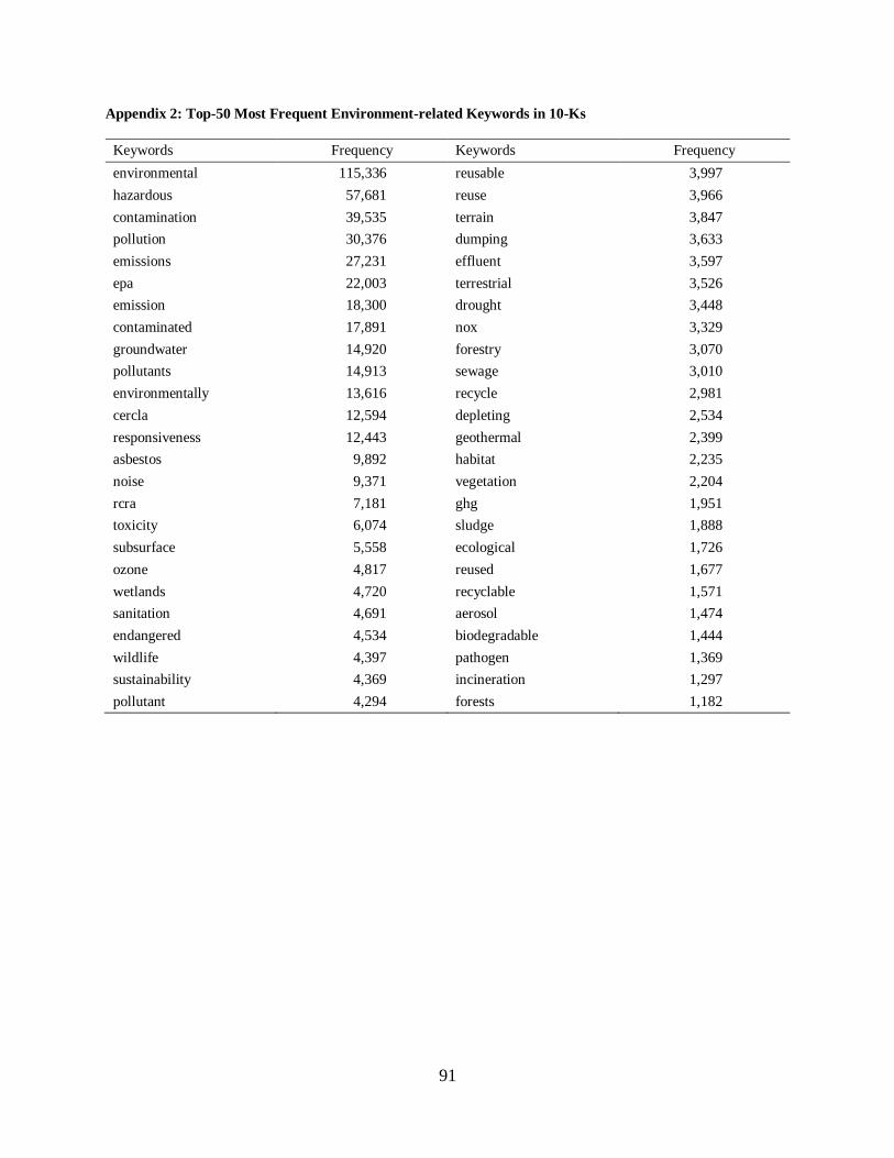
91

Appendix 2: Top-50 Most Frequent Environment-related Keywords in 10-Ks

Keywords Frequency Keywords Frequency

environmental 115,336 reusable 3,997

hazardous 57,681 reuse 3,966

contamination 39,535 terrain 3,847

pollution 30,376 dumping 3,633

emissions 27,231 effluent 3,597

epa 22,003 terrestrial 3,526

emission 18,300 drought 3,448

contaminated 17,891 nox 3,329

groundwater 14,920 forestry 3,070

pollutants 14,913 sewage 3,010

environmentally 13,616 recycle 2,981

cercla 12,594 depleting 2,534

responsiveness 12,443 geothermal 2,399

asbestos 9,892 habitat 2,235

noise 9,371 vegetation 2,204

rcra 7,181 ghg 1,951

toxicity 6,074 sludge 1,888

subsurface 5,558 ecological 1,726

ozone 4,817 reused 1,677

wetlands 4,720 recyclable 1,571

sanitation 4,691 aerosol 1,474

endangered 4,534 biodegradable 1,444

wildlife 4,397 pathogen 1,369

sustainability 4,369 incineration 1,297

pollutant 4,294 forests 1,182

92

Appendix 3: Examples of Sentences containing Environment-related Keywords

Keywords Examples

Environmental “Future closure, reclamation and environmental related expenditures are difficult to estimate

in many circumstances due to the early stages of investigation, uncertainties …”

Hazardous “Some of the Company’s current and former facilities are the subject of environmental investigations and remediations resulting from historical operations and the release of

hazardous substances or other constituents.”

Contamination "The Company believes that none of its activities caused contamination at the Site, and will

contest this claim by EPA and therefore no liability has been accrued for this matter."

Pollution "Population growth, increasing per capita demand for electric power in emerging markets,

and pollution from coal-fired plants further provide a strong foundation for increased demand

for nuclear fuel."

EPA "In April 2012, the EPA proposed new source performance standards for new fossil-fueled

generating facilities that would limit emissions of carbon dioxide to 1,000 pounds per MWh."

CERCLA "The decision establishes that Appleton is no longer a PRP, no longer liable under the federal

Comprehensive Environmental Response, Compensation, and Liability Act, (“CERCLA” or

“Superfund”),…"

Asbestos “As discussed more fully in Note 18 of the notes to our consolidated financial statements, we

are responsible for certain future liabilities relating to alleged exposure to asbestos containing

products.”

Ozone "Until the states have developed implementation plans for the new NOx, SO2 and ozone

standards, it is not possible to determine the impact on Dominion?"

Pollutants "Final MACT Rule: The CAA requires the EPA to develop industry-based standards to control emissions of hazardous air pollutants, or HAPs."

Effluent “Environmental Initiatives: There are proposed legislation, rules and initiatives involving

matters related to air emissions, water effluent, hazardous materials and greenhouse gases, all

of which affect generation plant capital expenditures and operating costs as well as future

operational planning.”

GHG “Similar regulations exist at the federal level which require compliance related to greenhouse

gas (GHG) emissions and also allow for the sale of excess credits by one manufacturer to

other manufacturers.”

Recycles “The company manufactures and recycles a variety of pallets types as well as boxes.”

Oil spill “In the event of an oil spill or containment event, the appropriate OSRP and Containment

Plan would be executed as needed.”

Climate change “The physical impacts of climate change present potential risks for severe weather (floods,

hurricanes, tornadoes, etc.) at certain of the Company?”

Carbon dioxide “In 2010, the most recent year reported, carbon dioxide (CO2), a byproduct of all sources of

combustion, accounted for approximately 84 percent of total U.S.”

Global warming “Countermeasures being sought to limit global warming are expected to favor the

deployment of alternative energy technologies.”

Kyoto Protocol “The current international climate framework, the United Nations-sponsored Kyoto Protocol,

prescribes specific targets to reduce GHG emissions for developed countries for the 2008-

2012 period.”

Carbon dioxide “Congress has considered establishing a cap-and-trade program to reduce U.S. emissions of

greenhouse gases, including carbon dioxide and methane.”

Clean Air “The Clean Air Act is a federal law administered by the EPA that provides a framework for

protecting and improving the nation's air quality and controlling sources of air emissions.”

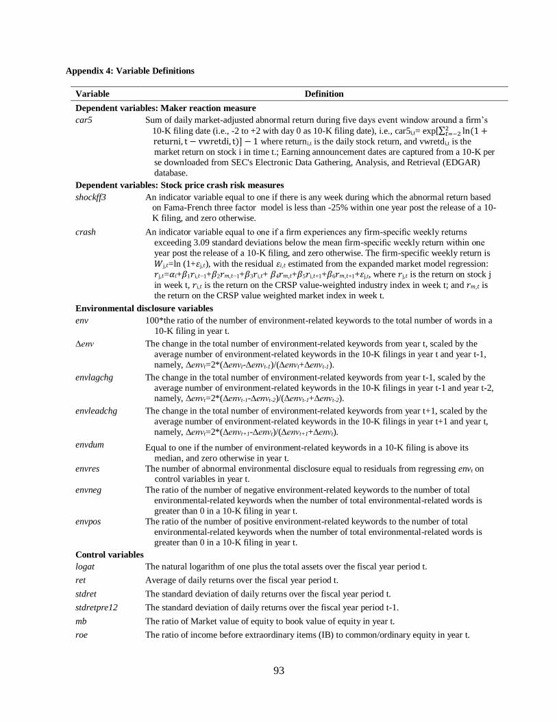
93

Appendix 4: Variable Definitions

Variable Definition

Dependent variables: Maker reaction measure

car5 Sum of daily market-adjusted abnormal return during five days event window around a firm’s

10-K filing date (i.e., -2 to +2 with day 0 as 10-K filing date), i.e., car5i,t= exp[∑ ln(1 +2𝑡=−2

returni, t − vwretdi, t)] − 1 where returni,t is the daily stock return, and vwretdi,t is the

market return on stock i in time t.; Earning announcement dates are captured from a 10-K per

se downloaded from SEC's Electronic Data Gathering, Analysis, and Retrieval (EDGAR)

database.

Dependent variables: Stock price crash risk measures

shockff3 An indicator variable equal to one if there is any week during which the abnormal return based on Fama-French three factor model is less than -25% within one year post the release of a 10-

K filing, and zero otherwise.

crash An indicator variable equal to one if a firm experiences any firm-specific weekly returns

exceeding 3.09 standard deviations below the mean firm-specific weekly return within one

year post the release of a 10-K filing, and zero otherwise. The firm-specific weekly return is

𝑊j,𝑡=ln (1+𝜀j,𝑡), with the residual 𝜀𝑖,𝑡 estimated from the expanded market model regression:

𝑟j,𝑡=𝛼𝑖+𝛽1𝑟i,𝑡−1+𝛽2𝑟𝑚,𝑡−1+𝛽3𝑟i,𝑡+ 𝛽4𝑟𝑚,𝑡+𝛽5𝑟i,𝑡+1+𝛽6𝑟𝑚,𝑡+1+𝜀j,t, where 𝑟j,𝑡 is the return on stock j

in week t, 𝑟i,𝑡 is the return on the CRSP value-weighted industry index in week t; and 𝑟𝑚,𝑡 is

the return on the CRSP value weighted market index in week t.

Environmental disclosure variables

env 100*the ratio of the number of environment-related keywords to the total number of words in a

10-K filing in year t.

∆env The change in the total number of environment-related keywords from year t, scaled by the

average number of environment-related keywords in the 10-K filings in year t and year t-1,

namely, ∆envt=2*(∆envt-∆envt-1)/(∆envt+∆envt-1).

envlagchg The change in the total number of environment-related keywords from year t-1, scaled by the

average number of environment-related keywords in the 10-K filings in year t-1 and year t-2, namely, ∆envt=2*(∆envt-1-∆envt-2)/(∆envt-1+∆envt-2).

envleadchg The change in the total number of environment-related keywords from year t+1, scaled by the

average number of environment-related keywords in the 10-K filings in year t+1 and year t,

namely, ∆envt=2*(∆envt+1-∆envt)/(∆envt+1+∆envt).

envdum Equal to one if the number of environment-related keywords in a 10-K filing is above its

median, and zero otherwise in year t.

envres The number of abnormal environmental disclosure equal to residuals from regressing envt on control variables in year t.

envneg The ratio of the number of negative environment-related keywords to the number of total

environmental-related keywords when the number of total environmental-related words is

greater than 0 in a 10-K filing in year t.

envpos The ratio of the number of positive environment-related keywords to the number of total

environmental-related keywords when the number of total environmental-related words is

greater than 0 in a 10-K filing in year t.

Control variables

logat The natural logarithm of one plus the total assets over the fiscal year period t.

ret Average of daily returns over the fiscal year period t.

stdret The standard deviation of daily returns over the fiscal year period t.

stdretpre12 The standard deviation of daily returns over the fiscal year period t-1.

mb The ratio of Market value of equity to book value of equity in year t.

roe The ratio of income before extraordinary items (IB) to common/ordinary equity in year t.

94

leverage The ratio of total long-term debts to total assets in year t.

intangible The ratio of intangible assets to total assets in year t.

iholding Institutional holding is measured as the total number of shares held by institutions divided by

shares outstanding at the end of the same quarter in quarter t. The percentage holdings of

institutional investors are zero if no institutional investor reports positive holdings for a firm-

quarter.

totwords The natural logarithm of one plus the number of total words in 10-Ks in year t.

turnover Share trading volume, calculated as 100 times the number of shares traded for a firm deflated by

the total number of common shares outstanding in year t.

litigious The ratio of the number of litigation-related keywords to the total number of words in a 10-K

filing in year t.

esi Equal to one if a firm belongs to an environmentally sensitive industry which has the 2-digit

SIC code such as 13 (oil exploration), 26 (paper), 28 (chemical and allied products), 29 (petroleum refining), or 33 (metals), and zero otherwise.

hrtotwords The natural logarithm of one plus the total number of human right–related keywords in a 10-K

filing in year t.

retotwords The natural logarithm of one plus the total number of product responsibility–related keywords in

a 10-K filing in year t.

sototwords The natural logarithm of one plus the total number of society–related keywords in a 10-K filing in year t.

ncskewlag The negative skewness of firm-specific weekly returns over the fiscal year period.before the

release of a 10-K filing, calculated as by taking the negative of the third moment of firm-

specific weekly returns for each sample year and dividing it by the standard deviation of firm-

specific weekly returns raised to the third power.

em Magnitude of Earnings management measured as the absolute value of discretionary accruals

(Hutton et al. 2009)

ytrend Year trend which is equal to the year of the 10-K filing minus 1998.

Instrument variables

spill BP's Deepwater Horizon oil spill accident equal to one if year is after 2010, is missing for 2010,

and zero otherwise.

epa Massachusetts v. Environmental Protection Agency lawsuit equal to one if year is after 2007, is

missing for 2007, and zero otherwise.

Moderating variable

lognanalystdum Equal to one if lognanalyst is above its median, and 0 otherwise. lognanalyst is defined as a

natural logarithm of the number of analysts following the firm in year t.

Other variable

litigiousdum Equal to one if litigious is above its median, and zero otherwise.

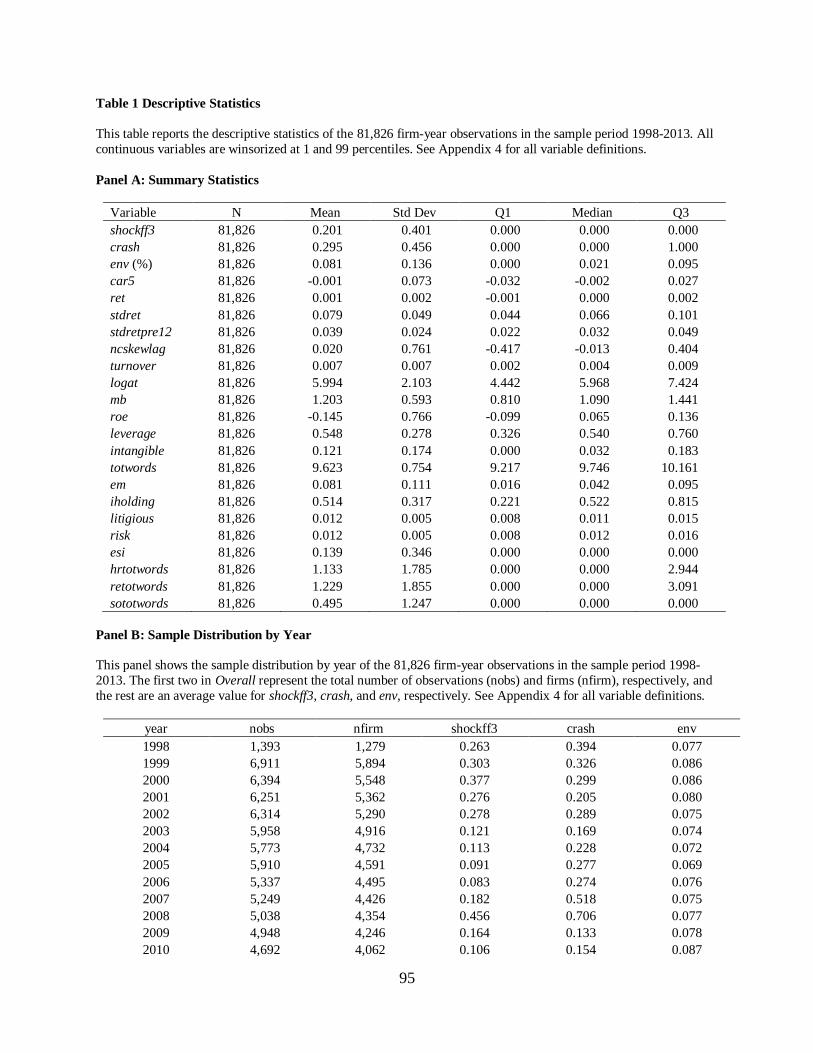
95

Table 1 Descriptive Statistics

This table reports the descriptive statistics of the 81,826 firm-year observations in the sample period 1998-2013. All

continuous variables are winsorized at 1 and 99 percentiles. See Appendix 4 for all variable definitions.

Panel A: Summary Statistics

Variable N Mean Std Dev Q1 Median Q3

shockff3 81,826 0.201 0.401 0.000 0.000 0.000

crash 81,826 0.295 0.456 0.000 0.000 1.000

env (%) 81,826 0.081 0.136 0.000 0.021 0.095

car5 81,826 -0.001 0.073 -0.032 -0.002 0.027

ret 81,826 0.001 0.002 -0.001 0.000 0.002

stdret 81,826 0.079 0.049 0.044 0.066 0.101

stdretpre12 81,826 0.039 0.024 0.022 0.032 0.049

ncskewlag 81,826 0.020 0.761 -0.417 -0.013 0.404

turnover 81,826 0.007 0.007 0.002 0.004 0.009

logat 81,826 5.994 2.103 4.442 5.968 7.424

mb 81,826 1.203 0.593 0.810 1.090 1.441

roe 81,826 -0.145 0.766 -0.099 0.065 0.136

leverage 81,826 0.548 0.278 0.326 0.540 0.760

intangible 81,826 0.121 0.174 0.000 0.032 0.183

totwords 81,826 9.623 0.754 9.217 9.746 10.161

em 81,826 0.081 0.111 0.016 0.042 0.095

iholding 81,826 0.514 0.317 0.221 0.522 0.815

litigious 81,826 0.012 0.005 0.008 0.011 0.015

risk 81,826 0.012 0.005 0.008 0.012 0.016

esi 81,826 0.139 0.346 0.000 0.000 0.000

hrtotwords 81,826 1.133 1.785 0.000 0.000 2.944

retotwords 81,826 1.229 1.855 0.000 0.000 3.091

sototwords 81,826 0.495 1.247 0.000 0.000 0.000

Panel B: Sample Distribution by Year

This panel shows the sample distribution by year of the 81,826 firm-year observations in the sample period 1998-

2013. The first two in Overall represent the total number of observations (nobs) and firms (nfirm), respectively, and

the rest are an average value for shockff3, crash, and env, respectively. See Appendix 4 for all variable definitions.

year nobs nfirm shockff3 crash env

1998 1,393 1,279 0.263 0.394 0.077

1999 6,911 5,894 0.303 0.326 0.086

2000 6,394 5,548 0.377 0.299 0.086

2001 6,251 5,362 0.276 0.205 0.080

2002 6,314 5,290 0.278 0.289 0.075

2003 5,958 4,916 0.121 0.169 0.074

2004 5,773 4,732 0.113 0.228 0.072

2005 5,910 4,591 0.091 0.277 0.069

2006 5,337 4,495 0.083 0.274 0.076

2007 5,249 4,426 0.182 0.518 0.075

2008 5,038 4,354 0.456 0.706 0.077

2009 4,948 4,246 0.164 0.133 0.078

2010 4,692 4,062 0.106 0.154 0.087

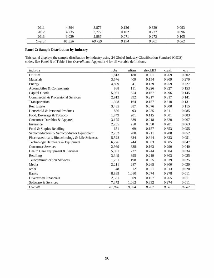
96

2011 4,394 3,876 0.126 0.329 0.093

2012 4,235 3,772 0.102 0.237 0.096

2013 3,029 2,886 0.071 0.273 0.105

Overall 81,826 69,729 0.194 0.301 0.082

Panel C: Sample Distribution by Industry

This panel displays the sample distribution by industry using 24 Global Industry Classification Standard (GICS)

codes. See Panel B of Table 1 for Overall, and Appendix 4 for all variable definitions.

industry nobs nfirm shockff3 crash env

Utilities 1,813 180 0.061 0.269 0.302

Materials 3,576 409 0.154 0.309 0.270

Energy 4,899 541 0.139 0.259 0.227

Automobiles & Components 868 111 0.226 0.327 0.153

Capital Goods 5,931 654 0.167 0.296 0.145

Commercial & Professional Services 2,913 392 0.217 0.317 0.141

Transportation 1,398 164 0.157 0.310 0.131

Real Estate 3,485 387 0.076 0.300 0.115

Household & Personal Products 856 93 0.235 0.311 0.085

Food, Beverage & Tobacco 1,749 201 0.115 0.301 0.083

Consumer Durables & Apparel 3,175 389 0.218 0.320 0.067

Insurance 2,235 250 0.090 0.281 0.063

Food & Staples Retailing 651 69 0.157 0.353 0.055

Semiconductors & Semiconductor Equipment 2,252 208 0.211 0.288 0.052

Pharmaceuticals, Biotechnology & Life Sciences 5,528 634 0.344 0.323 0.051

Technology Hardware & Equipment 6,226 744 0.303 0.305 0.047

Consumer Services 2,989 338 0.163 0.290 0.040

Health Care Equipment & Services 5,901 727 0.244 0.304 0.034

Retailing 3,349 395 0.219 0.303 0.025

Telecommunication Services 1,231 198 0.335 0.339 0.025

Media 2,211 287 0.265 0.300 0.020

other 48 12 0.521 0.313 0.020

Banks 8,839 1,080 0.074 0.278 0.011

Diversified Financials 2,331 309 0.157 0.265 0.011

Software & Services 7,372 1,062 0.332 0.274 0.011

Overall 81,826 9,834 0.207 0.301 0.087

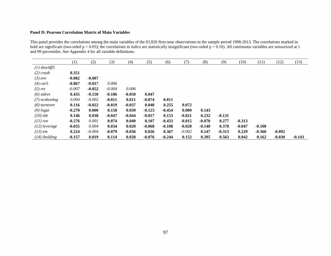
97

Panel D: Pearson Correlation Matrix of Main Variables

This panel provides the correlations among the main variables of the 81,826 firm-year observations in the sample period 1998-2013. The correlations marked in

bold are significant (two-sided p < 0.05); the correlations in italics are statistically insignificant (two-sided p > 0.10). All continuous variables are winsorized at 1

and 99 percentiles. See Appendix 4 for all variable definitions.

(1) (2) (3) (4) (5) (6) (7) (8) (9) (10) (11) (12) (13)

(1) shockff3

(2) crash 0.351

(3) env -0.082 -0.007

(4) car5 -0.067 -0.017 0.006

(5) ret -0.007 -0.052 -0.004 0.006

(6) stdret 0.435 -0.150 -0.106 -0.050 0.047

(7) ncskewlag 0.004 -0.002 -0.011 0.011 -0.074 0.011

(8) turnover 0.116 -0.022 -0.019 -0.037 0.040 0.255 0.072

(9) logat -0.270 0.000 0.158 0.039 -0.123 -0.454 0.089 0.143

(10) mb 0.146 0.038 -0.047 -0.044 -0.017 0.153 -0.021 0.232 -0.131

(11) roe -0.276 0.001 0.074 0.049 0.107 -0.433 -0.015 -0.070 0.277 -0.313

(12) leverage -0.035 0.004 0.034 0.020 -0.068 -0.108 -0.020 -0.140 0.378 -0.047 -0.100

(13) em 0.224 -0.004 -0.079 -0.036 0.026 0.367 -0.002 0.147 -0.313 0.229 -0.360 -0.092

(14) iholding -0.157 0.019 0.114 0.028 -0.076 -0.244 0.152 0.395 0.563 0.042 0.162 -0.030 -0.143

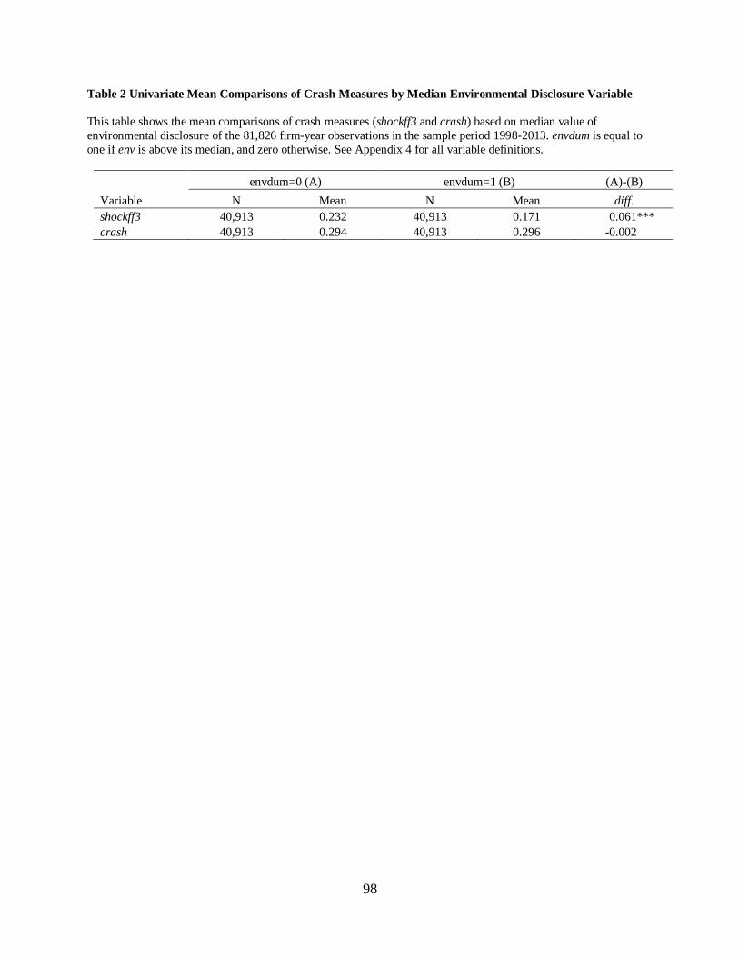
98

Table 2 Univariate Mean Comparisons of Crash Measures by Median Environmental Disclosure Variable

This table shows the mean comparisons of crash measures (shockff3 and crash) based on median value of

environmental disclosure of the 81,826 firm-year observations in the sample period 1998-2013. envdum is equal to

one if env is above its median, and zero otherwise. See Appendix 4 for all variable definitions.

envdum=0 (A) envdum=1 (B) (A)-(B)

Variable N Mean N Mean diff.

shockff3 40,913 0.232 40,913 0.171 0.061***

crash 40,913 0.294 40,913 0.296 -0.002

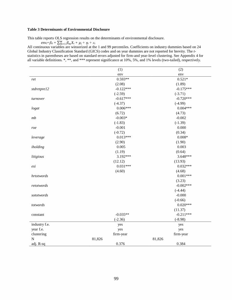
99

Table 3 Determinants of Environmental Disclosure

This table reports OLS regression results on the determinants of environmental disclosure.

envt=β0 + ∑ 𝛽𝑚𝑀𝑚=1 Xt + µ j + ŋt + εt

All continuous variables are winsorized at the 1 and 99 percentiles. Coefficients on industry dummies based on 24

Global Industry Classification Standard (GICS) codes and on year dummies are not reported for brevity. The t-

statistics in parentheses are based on standard errors adjusted for firm-and year-level clustering. See Appendix 4 for

all variable definitions. *, **, and *** represent significance at 10%, 5%, and 1% levels (two-tailed), respectively.

(1) (2)

env env

ret 0.593** 0.521*

(2.08) (1.89)

stdretpre12 -0.122*** -0.175***

(-2.59) (-3.71)

turnover -0.617*** -0.720***

(-4.37) (-4.99)

logat 0.006*** 0.004***

(6.72) (4.73)

mb -0.003* -0.002

(-1.83) (-1.39)

roe -0.001 0.000

(-0.72) (0.34)

leverage 0.013*** 0.008*

(2.90) (1.90)

iholding 0.005 0.003

(1.19) (0.64)

litigious 3.192*** 3.648***

(12.12) (13.93)

esi 0.031*** 0.032***

(4.60) (4.68)

hrtotwords 0.001***

(3.23)

retotwords -0.002***

(-4.44)

sototwords -0.000

(-0.66)

totwords 0.020***

(11.37)

constant -0.035** -0.211***

(-2.36) (-8.98)

industry f.e. yes yes

year f.e. yes yes

clustering firm-year firm-year

N 81,826 81,826

adj. R-sq 0.376 0.384

100

Table 4 Evidence of Environmental Disclosure as Bad News

Panel A: Correlation between Environmental Disclosure and Litigation

See Panel D of Table 1 for the correlation table and Appendix 4 for all variable definitions.

env

litigious 0.200

Panel B: Univariate Mean Comparisons of Environmental Disclosure by Median Litigation Variable

This panel shows the mean comparisons of environmental disclosure measure (env) based on median value of

litigation variable of the 81,826 firm-year observations in the sample period 1998-2013. litigiousdum is equal to one

if litigious is above its median, and zero otherwise. See Appendix 4 for all variable definitions.

litigiousdum=0 (A) litigiousdum=1 (B) (A)-(B)

Variable N Mean N Mean diff.

env 40,913 0.054 40,913 0.107 -0.053***

Panel C: Mean Reversal of Change in Environmental Disclosure

See Panel D of Table 1 for the correlation table. ∆envlag (∆envlead) is the difference between ∆env and previous

(next)-period ∆env. See Appendix 4 for all variable definitions.

Panel D: Summary Statistics of Negative vs. Positive Environmental Disclosure

See Appendix 4 for all variable definitions.

Variable N Mean Std Dev Q1 Median Q3

envneg 24,433 0.034 0.038 0.000 0.023 0.051

envpos 10,918 0.022 0.023 0.007 0.013 0.026

∆env ∆envlag

∆env

∆envlag -0.141

∆envlead -0.235 0.104

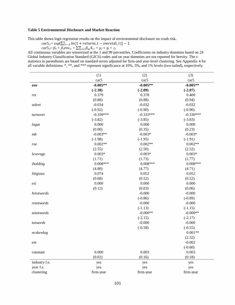
101

Table 5 Environmental Disclosure and Market Reaction

This table shows logit regression results on the impact of environmental disclosure on crash risk.

car5i,t= exp[∑ 𝑙𝑛(1 + 𝑟𝑒𝑡𝑢𝑟𝑛𝑖, 𝑡 − 𝑣𝑤𝑟𝑒𝑡𝑑𝑖, 𝑡)] − 12𝑡=−2

car5i,t=β0 + β1envi,t + ∑ 𝛽𝑚𝑀𝑚=2 Xi,t + µ j + ŋt + εt

All continuous variables are winsorized at the 1 and 99 percentiles. Coefficients on industry dummies based on 24

Global Industry Classification Standard (GICS) codes and on year dummies are not reported for brevity. The t-

statistics in parentheses are based on standard errors adjusted for firm-and year-level clustering. See Appendix 4 for all variable definitions. *, **, and *** represent significance at 10%, 5%, and 1% levels (two-tailed), respectively.

(1) (2) (3)

car5 car5 car5

env -0.005** -0.005** -0.005**

(-2.38) (-2.09) (-2.07)

ret 0.379 0.378 0.400

(0.88) (0.88) (0.94)

stdret -0.034 -0.032 -0.032

(-0.92) (-0.90) (-0.90)

turnover -0.339*** -0.333*** -0.330***

(-3.82) (-3.85) (-3.83)

logat 0.000 0.000 0.000

(0.00) (0.35) (0.23)

mb -0.003** -0.003* -0.003*

(-1.98) (-1.95) (-1.91)

roe 0.002** 0.002** 0.002**

(2.55) (2.50) (2.52)

leverage 0.003* 0.003* 0.003*

(1.71) (1.73) (1.77)

iholding 0.008*** 0.008*** 0.008***

(4.80) (4.77) (4.71)

litigious 0.074 0.052 0.052

(0.68) (0.52) (0.52)

esi 0.000 0.000 0.000

(0.12) (0.03) (0.06)

hrtotwords -0.000 -0.000

(-0.86) (-0.89)

retotwords -0.000 -0.000

(-1.13) (-1.15)

sototwords -0.000** -0.000**

(-2.15) (-2.17)

totwords -0.000 -0.000

(-0.58) (-0.55)

ncskewlag 0.001**

(2.32)

em -0.002

(-0.60)

constant 0.000 0.003 0.003

(0.02) (0.16) (0.18)

industry f.e. yes yes yes

year f.e. yes yes yes

clustering firm-year firm-year firm-year

102

N 81,826 81,826 81,826

adj. R-sq 0.007 0.007 0.007

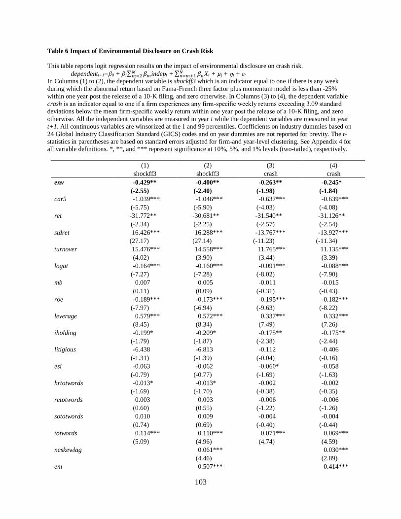
103

Table 6 Impact of Environmental Disclosure on Crash Risk

This table reports logit regression results on the impact of environmental disclosure on crash risk.

dependentt+1=β0 + β1∑ 𝛽𝑚𝑀𝑚=2 indept + ∑ 𝛽𝑛

𝑁𝑛=𝑚+1 Xt + µ j + ŋt + εt

In Columns (1) to (2), the dependent variable is shockff3 which is an indicator equal to one if there is any week

during which the abnormal return based on Fama-French three factor plus momentum model is less than -25%

within one year post the release of a 10-K filing, and zero otherwise. In Columns (3) to (4), the dependent variable

crash is an indicator equal to one if a firm experiences any firm-specific weekly returns exceeding 3.09 standard

deviations below the mean firm-specific weekly return within one year post the release of a 10-K filing, and zero

otherwise. All the independent variables are measured in year t while the dependent variables are measured in year

t+1. All continuous variables are winsorized at the 1 and 99 percentiles. Coefficients on industry dummies based on

24 Global Industry Classification Standard (GICS) codes and on year dummies are not reported for brevity. The t-

statistics in parentheses are based on standard errors adjusted for firm-and year-level clustering. See Appendix 4 for all variable definitions. *, **, and *** represent significance at 10%, 5%, and 1% levels (two-tailed), respectively.

(1) (2) (3) (4)

shockff3 shockff3 crash crash

env -0.429** -0.400** -0.263** -0.245*

(-2.55) (-2.40) (-1.98) (-1.84)

car5 -1.039*** -1.046*** -0.637*** -0.639***

(-5.75) (-5.90) (-4.03) (-4.08)

ret -31.772** -30.681** -31.540** -31.126**

(-2.34) (-2.25) (-2.57) (-2.54)

stdret 16.426*** 16.288*** -13.767*** -13.927***

(27.17) (27.14) (-11.23) (-11.34)

turnover 15.476*** 14.558*** 11.765*** 11.135***

(4.02) (3.90) (3.44) (3.39)

logat -0.164*** -0.160*** -0.091*** -0.088***

(-7.27) (-7.28) (-8.02) (-7.90)

mb 0.007 0.005 -0.011 -0.015

(0.11) (0.09) (-0.31) (-0.43)

roe -0.189*** -0.173*** -0.195*** -0.182***

(-7.97) (-6.94) (-9.63) (-8.22)

leverage 0.579*** 0.572*** 0.337*** 0.332***

(8.45) (8.34) (7.49) (7.26)

iholding -0.199* -0.209* -0.175** -0.175**

(-1.79) (-1.87) (-2.38) (-2.44)

litigious -6.438 -6.813 -0.112 -0.406

(-1.31) (-1.39) (-0.04) (-0.16)

esi -0.063 -0.062 -0.060* -0.058

(-0.79) (-0.77) (-1.69) (-1.63)

hrtotwords -0.013* -0.013* -0.002 -0.002

(-1.69) (-1.70) (-0.38) (-0.35)

retotwords 0.003 0.003 -0.006 -0.006

(0.60) (0.55) (-1.22) (-1.26)

sototwords 0.010 0.009 -0.004 -0.004

(0.74) (0.69) (-0.40) (-0.44)

totwords 0.114*** 0.110*** 0.071*** 0.069***

(5.09) (4.96) (4.74) (4.59)

ncskewlag 0.061*** 0.030***

(4.46) (2.89)

em 0.507*** 0.414***

104

(3.55) (2.99)

constant -1.971*** -1.976*** 0.695 0.695

(-3.60) (-3.65) (1.38) (1.37)

industry f.e. yes yes yes yes

year f.e. yes yes yes yes

clustering firm-year firm-year firm-year firm-year

N 81,826 81,826 81,826 81,826

Log likelihood -30075.527 -30049.609 -44693.934 -44678.691

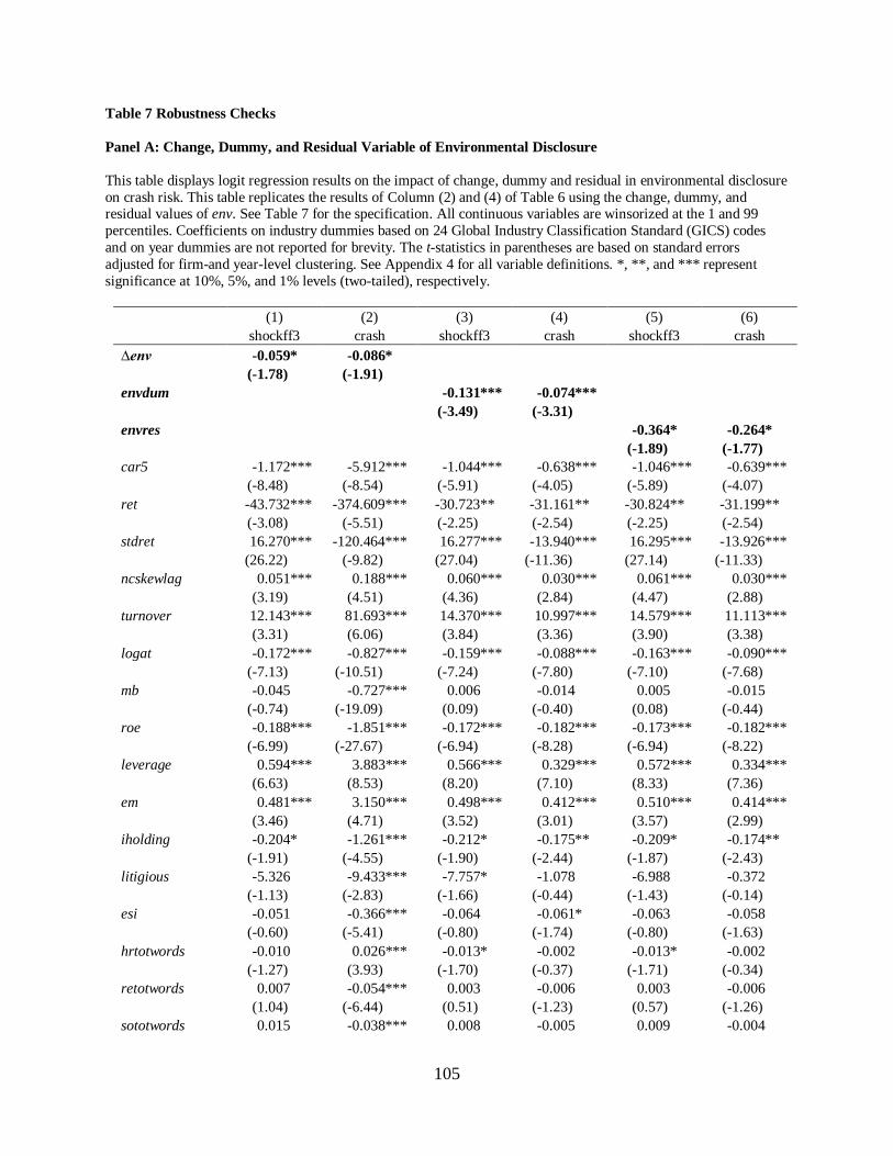
105

Table 7 Robustness Checks

Panel A: Change, Dummy, and Residual Variable of Environmental Disclosure

This table displays logit regression results on the impact of change, dummy and residual in environmental disclosure

on crash risk. This table replicates the results of Column (2) and (4) of Table 6 using the change, dummy, and residual values of env. See Table 7 for the specification. All continuous variables are winsorized at the 1 and 99

percentiles. Coefficients on industry dummies based on 24 Global Industry Classification Standard (GICS) codes

and on year dummies are not reported for brevity. The t-statistics in parentheses are based on standard errors

adjusted for firm-and year-level clustering. See Appendix 4 for all variable definitions. *, **, and *** represent

significance at 10%, 5%, and 1% levels (two-tailed), respectively.

(1) (2) (3) (4) (5) (6)

shockff3 crash shockff3 crash shockff3 crash

∆env -0.059* -0.086*

(-1.78) (-1.91)

envdum -0.131*** -0.074***

(-3.49) (-3.31)

envres -0.364* -0.264*

(-1.89) (-1.77)

car5 -1.172*** -5.912*** -1.044*** -0.638*** -1.046*** -0.639***

(-8.48) (-8.54) (-5.91) (-4.05) (-5.89) (-4.07)

ret -43.732*** -374.609*** -30.723** -31.161** -30.824** -31.199**

(-3.08) (-5.51) (-2.25) (-2.54) (-2.25) (-2.54)

stdret 16.270*** -120.464*** 16.277*** -13.940*** 16.295*** -13.926***

(26.22) (-9.82) (27.04) (-11.36) (27.14) (-11.33)

ncskewlag 0.051*** 0.188*** 0.060*** 0.030*** 0.061*** 0.030***

(3.19) (4.51) (4.36) (2.84) (4.47) (2.88)

turnover 12.143*** 81.693*** 14.370*** 10.997*** 14.579*** 11.113***

(3.31) (6.06) (3.84) (3.36) (3.90) (3.38)

logat -0.172*** -0.827*** -0.159*** -0.088*** -0.163*** -0.090***

(-7.13) (-10.51) (-7.24) (-7.80) (-7.10) (-7.68)

mb -0.045 -0.727*** 0.006 -0.014 0.005 -0.015

(-0.74) (-19.09) (0.09) (-0.40) (0.08) (-0.44)

roe -0.188*** -1.851*** -0.172*** -0.182*** -0.173*** -0.182***

(-6.99) (-27.67) (-6.94) (-8.28) (-6.94) (-8.22)

leverage 0.594*** 3.883*** 0.566*** 0.329*** 0.572*** 0.334***

(6.63) (8.53) (8.20) (7.10) (8.33) (7.36)

em 0.481*** 3.150*** 0.498*** 0.412*** 0.510*** 0.414***

(3.46) (4.71) (3.52) (3.01) (3.57) (2.99)

iholding -0.204* -1.261*** -0.212* -0.175** -0.209* -0.174**

(-1.91) (-4.55) (-1.90) (-2.44) (-1.87) (-2.43)

litigious -5.326 -9.433*** -7.757* -1.078 -6.988 -0.372

(-1.13) (-2.83) (-1.66) (-0.44) (-1.43) (-0.14)

esi -0.051 -0.366*** -0.064 -0.061* -0.063 -0.058

(-0.60) (-5.41) (-0.80) (-1.74) (-0.80) (-1.63)

hrtotwords -0.010 0.026*** -0.013* -0.002 -0.013* -0.002

(-1.27) (3.93) (-1.70) (-0.37) (-1.71) (-0.34)

retotwords 0.007 -0.054*** 0.003 -0.006 0.003 -0.006

(1.04) (-6.44) (0.51) (-1.23) (0.57) (-1.26)

sototwords 0.015 -0.038*** 0.008 -0.005 0.009 -0.004

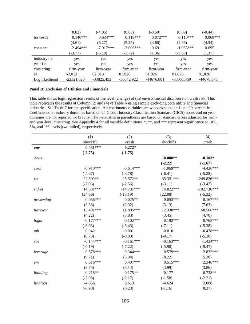
106

(0.82) (-4.05) (0.63) (-0.50) (0.69) (-0.44)

totwords 0.140*** 0.634*** 0.119*** 0.072*** 0.110*** 0.069***

(4.61) (6.27) (5.25) (4.86) (4.86) (4.54)

constant -2.494*** -7.917*** -2.006*** 0.691 -1.966*** 0.695

(-3.77) (-5.10) (-3.72) (1.36) (-3.63) (1.37)

industry f.e. yes yes yes yes yes yes

year f.e. yes yes yes yes yes yes

clustering firm-year firm-year firm-year firm-year firm-year firm-year

N 62,013 62,013 81,826 81,826 81,826 81,826

Log likelihood -22321.023 -33825.453 -30042.922 -44676.881 -30051.459 -44678.375

Panel B: Exclusion of Utilities and Financials

This table shows logit regression results of the level (change) of (in) environmental disclosure on crash risk. This

table replicates the results of Column (2) and (4) of Table 6 using sample excluding both utility and financial

industries. See Table 7 for the specification. All continuous variables are winsorized at the 1 and 99 percentiles.

Coefficients on industry dummies based on 24 Global Industry Classification Standard (GICS) codes and on year

dummies are not reported for brevity. The t-statistics in parentheses are based on standard errors adjusted for firm-

and year-level clustering. See Appendix 4 for all variable definitions. *, **, and *** represent significance at 10%,

5%, and 1% levels (two-tailed), respectively.

(1) (2) (3) (4)

shockff3 crash shockff3 crash

env -0.431*** -0.272*

(-2.75) (-1.75)

∆env -0.080** -0.103*

(-2.22) (-1.67)

car5 -0.910*** -0.614*** -1.069*** -4.426***

(-4.37) (-3.78) (-6.41) (-5.28)

ret -22.500** -25.572** -35.351*** -249.826***

(-2.06) (-2.56) (-3.11) (-3.42)

stdret 14.631*** -14.731*** 14.822*** -102.736***

(24.66) (-13.19) (22.08) (-5.32)

ncskewlag 0.056*** 0.025** 0.053*** 0.167***

(3.88) (2.32) (3.13) (7.63)

turnover 15.401*** 11.805*** 12.338*** 68.506***

(4.22) (3.83) (3.45) (4.70)

logat -0.177*** -0.102*** -0.192*** -0.765***

(-6.93) (-8.43) (-7.11) (-5.38)

mb 0.042 -0.001 -0.010 -0.478***

(0.73) (-0.03) (-0.17) (-5.38)

roe -0.144*** -0.161*** -0.163*** -1.424***

(-6.19) (-7.22) (-5.90) (-9.47)

leverage 0.578*** 0.344*** 0.579*** 2.832***

(9.71) (5.94) (8.22) (5.38)

em 0.516*** 0.407*** 0.515*** 2.346***

(3.75) (3.14) (3.99) (3.86)

iholding -0.218** -0.175** -0.177 -0.738**

(-2.03) (-2.17) (-1.58) (-2.21)

litigious -4.666 0.613 -4.624 2.088

(-0.98) (0.23) (-1.16) (0.37)

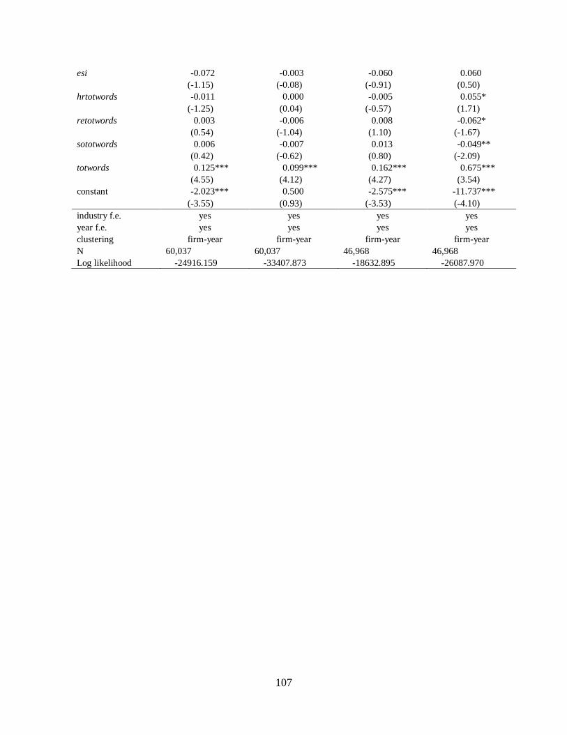
107

esi -0.072 -0.003 -0.060 0.060

(-1.15) (-0.08) (-0.91) (0.50)

hrtotwords -0.011 0.000 -0.005 0.055*

(-1.25) (0.04) (-0.57) (1.71)

retotwords 0.003 -0.006 0.008 -0.062*

(0.54) (-1.04) (1.10) (-1.67)

sototwords 0.006 -0.007 0.013 -0.049**

(0.42) (-0.62) (0.80) (-2.09)

totwords 0.125*** 0.099*** 0.162*** 0.675***

(4.55) (4.12) (4.27) (3.54)

constant -2.023*** 0.500 -2.575*** -11.737***

(-3.55) (0.93) (-3.53) (-4.10)

industry f.e. yes yes yes yes

year f.e. yes yes yes yes

clustering firm-year firm-year firm-year firm-year

N 60,037 60,037 46,968 46,968

Log likelihood -24916.159 -33407.873 -18632.895 -26087.970

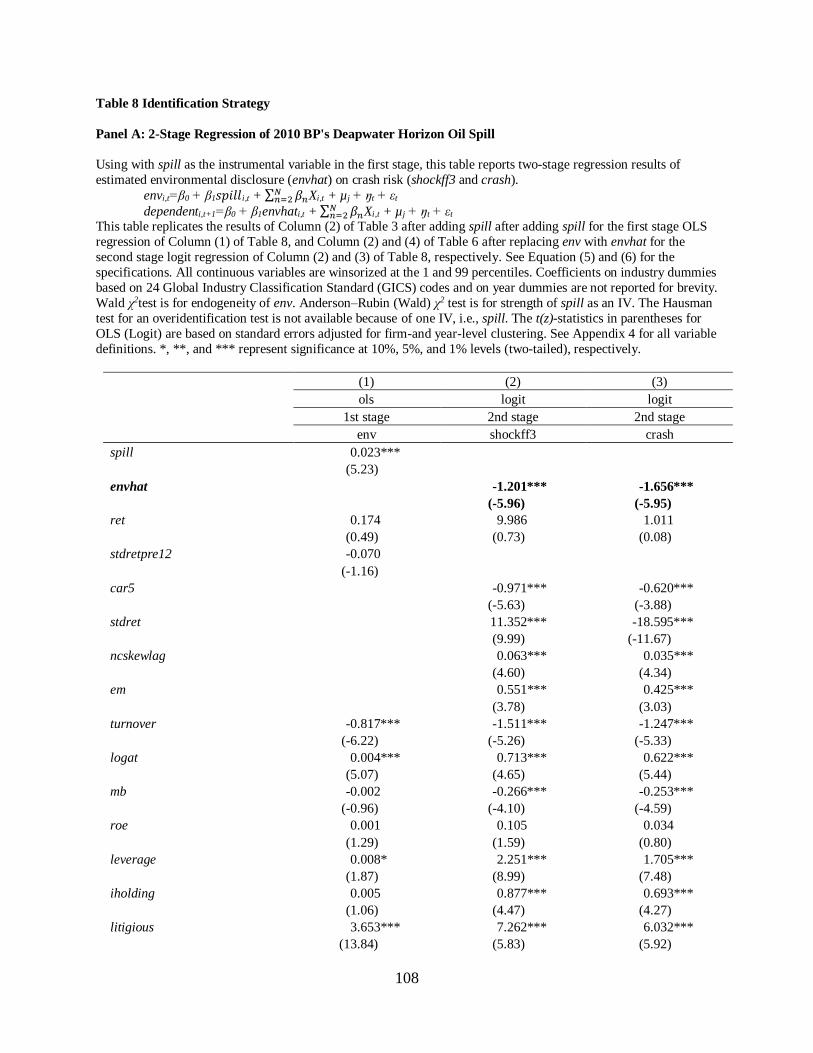
108

Table 8 Identification Strategy

Panel A: 2-Stage Regression of 2010 BP's Deapwater Horizon Oil Spill

Using with spill as the instrumental variable in the first stage, this table reports two-stage regression results of

estimated environmental disclosure (envhat) on crash risk (shockff3 and crash).

envi,t=β0 + β1𝑠𝑝𝑖𝑙𝑙i,t + ∑ 𝛽𝑛𝑁𝑛=2 Xi,t + µ j + ŋt + εt

dependenti,t+1=β0 + β1envhati,t + ∑ 𝛽𝑛𝑁𝑛=2 Xi,t + µ j + ŋt + εt

This table replicates the results of Column (2) of Table 3 after adding spill after adding spill for the first stage OLS

regression of Column (1) of Table 8, and Column (2) and (4) of Table 6 after replacing env with envhat for the

second stage logit regression of Column (2) and (3) of Table 8, respectively. See Equation (5) and (6) for the

specifications. All continuous variables are winsorized at the 1 and 99 percentiles. Coefficients on industry dummies

based on 24 Global Industry Classification Standard (GICS) codes and on year dummies are not reported for brevity.

Wald χ2test is for endogeneity of env. Anderson–Rubin (Wald) χ2 test is for strength of spill as an IV. The Hausman

test for an overidentification test is not available because of one IV, i.e., spill. The t(z)-statistics in parentheses for

OLS (Logit) are based on standard errors adjusted for firm-and year-level clustering. See Appendix 4 for all variable

definitions. *, **, and *** represent significance at 10%, 5%, and 1% levels (two-tailed), respectively.

(1) (2) (3)

ols logit logit

1st stage 2nd stage 2nd stage

env shockff3 crash

spill 0.023***

(5.23)

envhat -1.201*** -1.656***

(-5.96) (-5.95)

ret 0.174 9.986 1.011

(0.49) (0.73) (0.08)

stdretpre12 -0.070

(-1.16)

car5 -0.971*** -0.620***

(-5.63) (-3.88)

stdret 11.352*** -18.595***

(9.99) (-11.67)

ncskewlag 0.063*** 0.035***

(4.60) (4.34)

em 0.551*** 0.425***

(3.78) (3.03)

turnover -0.817*** -1.511*** -1.247***

(-6.22) (-5.26) (-5.33)

logat 0.004*** 0.713*** 0.622***

(5.07) (4.65) (5.44)

mb -0.002 -0.266*** -0.253***

(-0.96) (-4.10) (-4.59)

roe 0.001 0.105 0.034

(1.29) (1.59) (0.80)

leverage 0.008* 2.251*** 1.705***

(1.87) (8.99) (7.48)

iholding 0.005 0.877*** 0.693***

(1.06) (4.47) (4.27)

litigious 3.653*** 7.262*** 6.032***

(13.84) (5.83) (5.92)

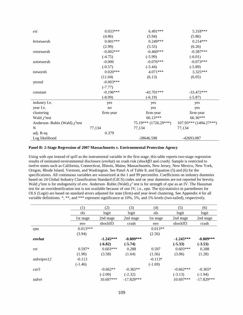
109

esi 0.033*** 6.491*** 5.318***

(4.86) (5.94) (5.86)

hrtotwords 0.001*** 0.249*** 0.214***

(2.99) (5.55) (6.26)

retotwords -0.002*** -0.460*** -0.387***

(-4.75) (-5.99) (-6.01)

sototwords -0.000 -0.076*** -0.073***

(-0.57) (-5.44) (-5.89)

totwords 0.020*** 4.071*** 3.325***

(11.04) (6.13) (6.05)

ytrend -0.003***

(-7.77)

constant -0.196*** -43.701*** -33.472***

(-8.09) (-6.19) (-5.87)

industry f.e. yes yes yes

year f.e. no yes yes

clustering firm-year firm-year firm-year

Wald χ2test 66.13*** 66.36***

Anderson–Rubin (Wald) χ2test 75.19*** (1726.29***) 107.95*** (1494.27***)

N 77,134 77,134 77,134

adj. R-sq 0.379

Log likelihood -28646.598 -42693.087

Panel B: 2-Stage Regression of 2007 Massachusetts v. Environmental Protection Agency

Using with epa instead of spill as the instrumental variable in the first stage, this table reports two-stage regression

results of estimated environmental disclosure (envhat) on crash risk (shockff3 and crash). Sample is restricted to twelve states such as California, Connecticut, Illinois, Maine, Massachusetts, New Jersey, New Mexico, New York,

Oregon, Rhode Island, Vermont, and Washington. See Panel A of Table 8, and Equation (5) and (6) for the

specifications. All continuous variables are winsorized at the 1 and 99 percentiles. Coefficients on industry dummies

based on 24 Global Industry Classification Standard (GICS) codes and on year dummies are not reported for brevity.

Wald χ2test is for endogeneity of env. Anderson–Rubin (Wald) χ2 test is for strength of epa as an IV. The Hausman

test for an overidentification test is not available because of one IV, i.e., epa. The t(z)-statistics in parentheses for

OLS (Logit) are based on standard errors adjusted for state (firm)-and year-level clustering. See Appendix 4 for all

variable definitions. *, **, and *** represent significance at 10%, 5%, and 1% levels (two-tailed), respectively.

(1) (2) (3) (4) (5) (6)

ols logit logit ols logit logit

1st stage 2nd stage 2nd stage 1st stage 2nd stage 2nd stage

env shockff3 crash env shockff3 crash

epa 0.013*** 0.013**

(3.94) (2.56)

envhat -1.245*** -0.809*** -1.245*** -0.809***

(-6.82) (-5.74) (-5.33) (-3.53)

ret 0.597* 0.603*** 0.288 0.597 0.603*** 0.288

(1.90) (3.58) (1.64) (1.56) (3.06) (1.28)

stdretpre12 -0.113 -0.113*

(-1.46) (-1.69)

car5 -0.662** -0.365** -0.662*** -0.365*

(-2.00) (-2.32) (-3.13) (-1.94)

stdret 10.697*** -17.829*** 10.697*** -17.829***

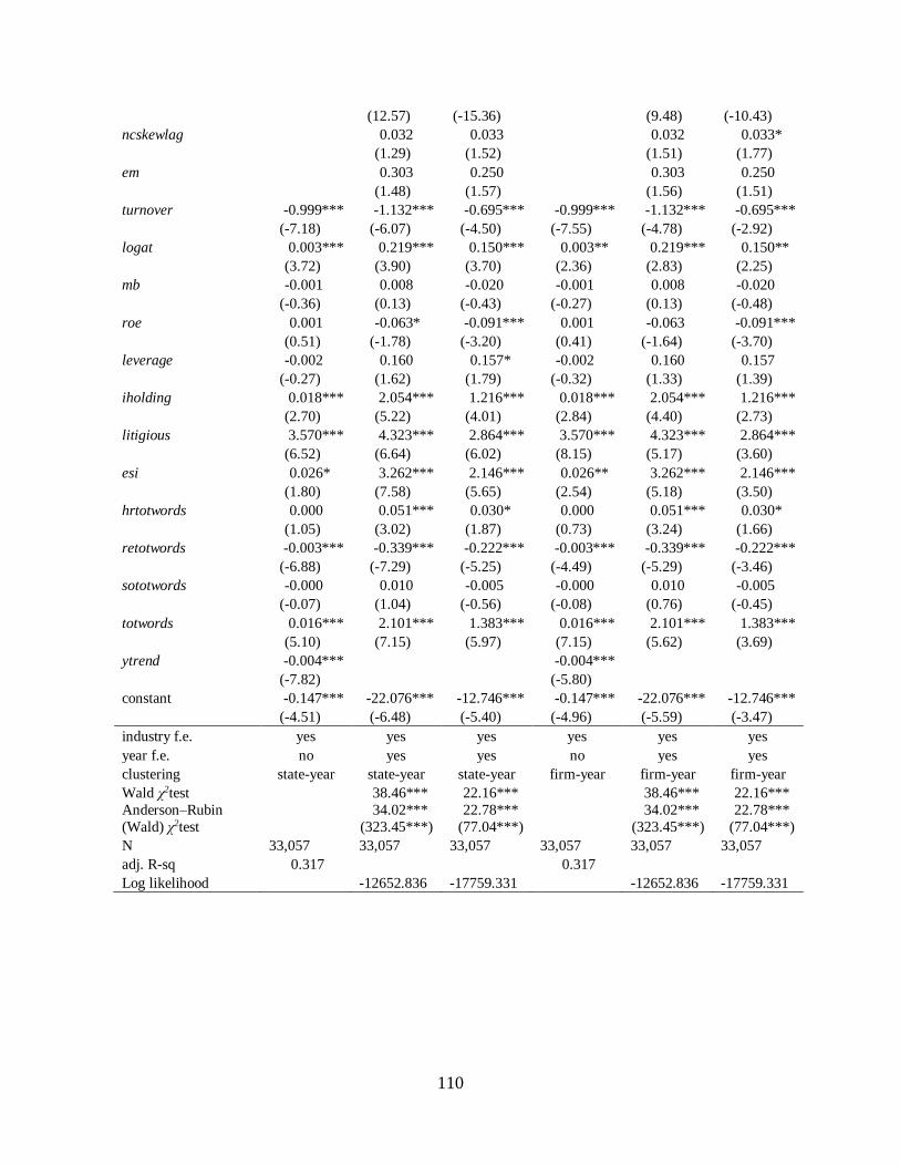
110

(12.57) (-15.36) (9.48) (-10.43)

ncskewlag 0.032 0.033 0.032 0.033*

(1.29) (1.52) (1.51) (1.77)

em 0.303 0.250 0.303 0.250

(1.48) (1.57) (1.56) (1.51)

turnover -0.999*** -1.132*** -0.695*** -0.999*** -1.132*** -0.695***

(-7.18) (-6.07) (-4.50) (-7.55) (-4.78) (-2.92)

logat 0.003*** 0.219*** 0.150*** 0.003** 0.219*** 0.150**

(3.72) (3.90) (3.70) (2.36) (2.83) (2.25)

mb -0.001 0.008 -0.020 -0.001 0.008 -0.020

(-0.36) (0.13) (-0.43) (-0.27) (0.13) (-0.48)

roe 0.001 -0.063* -0.091*** 0.001 -0.063 -0.091***

(0.51) (-1.78) (-3.20) (0.41) (-1.64) (-3.70)

leverage -0.002 0.160 0.157* -0.002 0.160 0.157

(-0.27) (1.62) (1.79) (-0.32) (1.33) (1.39)

iholding 0.018*** 2.054*** 1.216*** 0.018*** 2.054*** 1.216***

(2.70) (5.22) (4.01) (2.84) (4.40) (2.73)

litigious 3.570*** 4.323*** 2.864*** 3.570*** 4.323*** 2.864***

(6.52) (6.64) (6.02) (8.15) (5.17) (3.60)

esi 0.026* 3.262*** 2.146*** 0.026** 3.262*** 2.146***

(1.80) (7.58) (5.65) (2.54) (5.18) (3.50)

hrtotwords 0.000 0.051*** 0.030* 0.000 0.051*** 0.030*

(1.05) (3.02) (1.87) (0.73) (3.24) (1.66)

retotwords -0.003*** -0.339*** -0.222*** -0.003*** -0.339*** -0.222***

(-6.88) (-7.29) (-5.25) (-4.49) (-5.29) (-3.46)

sototwords -0.000 0.010 -0.005 -0.000 0.010 -0.005

(-0.07) (1.04) (-0.56) (-0.08) (0.76) (-0.45)

totwords 0.016*** 2.101*** 1.383*** 0.016*** 2.101*** 1.383***

(5.10) (7.15) (5.97) (7.15) (5.62) (3.69)

ytrend -0.004*** -0.004***

(-7.82) (-5.80)

constant -0.147*** -22.076*** -12.746*** -0.147*** -22.076*** -12.746***

(-4.51) (-6.48) (-5.40) (-4.96) (-5.59) (-3.47)

industry f.e. yes yes yes yes yes yes

year f.e. no yes yes no yes yes

clustering state-year state-year state-year firm-year firm-year firm-year

Wald χ2test 38.46*** 22.16*** 38.46*** 22.16***

Anderson–Rubin

(Wald) χ2test

34.02***

(323.45***)

22.78***

(77.04***)

34.02***

(323.45***)

22.78***

(77.04***)

N 33,057 33,057 33,057 33,057 33,057 33,057

adj. R-sq 0.317 0.317

Log likelihood -12652.836 -17759.331 -12652.836 -17759.331

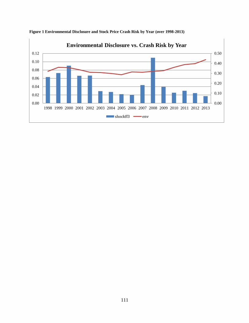
111

Figure 1 Environmental Disclosure and Stock Price Crash Risk by Year (over 1998-2013)

0.00

0.10

0.20

0.30

0.40

0.50

0.00

0.02

0.04

0.06

0.08

0.10

0.12

1998 1999 2000 2001 2002 2003 2004 2005 2006 2007 2008 2009 2010 2011 2012 2013

Environmental Disclosure vs. Crash Risk by Year

shockff3 env

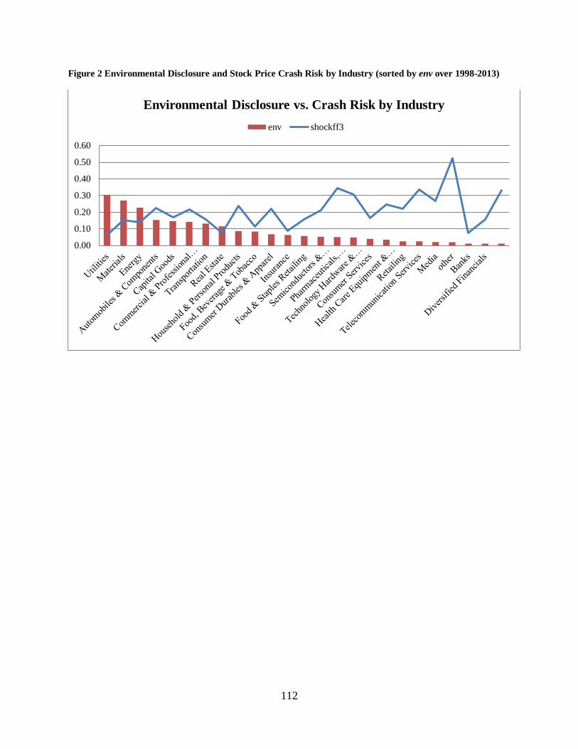
112

Figure 2 Environmental Disclosure and Stock Price Crash Risk by Industry (sorted by env over 1998-2013)

0.00

0.10

0.20

0.30

0.40

0.50

0.60

Environmental Disclosure vs. Crash Risk by Industry

env shockff3

113

Analyst Private Research Effort, Earnings Forecast Accuracy, and Market Reaction

Abstract

The study examines the relative value of private and public information sources in analysts’

earnings forecasts for U.S. firms. Using a pattern search algorithm (i.e., regular expression) on

the headlines of 81,762 forecasts during 2000-2014, the research significantly improves the

identification of information sources and finds that a forecast with an additional private source

has a higher accuracy and stronger market reaction. Moreover, the combination of a management

and non-management private source is more likely to generate the best accuracy and greatest

market reaction. Finally, more accurate and informative forecasts are made by analysts with

greater private research efforts even without information advantage. Overall, the study provides

new insight into the determinants of forecast properties.

Keywords: Private Research Effort, Private Information Source, Earnings Forecast Accuracy,

Market Reaction, Regular Expression

114

1. Introduction

“What is the source of that value-added?” Lo (2012) makes the question in that average

equity analysts are well-paid and thus, are expected to produce significant value-added outputs.23

24 The research answers the question, finding that it is an additional private information source.25

Depending on the availability of a public information source, equity analysts include

private (or proprietary) and/or public information as an input source of their research reports.

They are well equipped with the expertise to collect and process information into various types

of outputs for the report users, for example, stock recommendations, earnings forecasts, and

price targets. As such, analysts play an important intermediary role between a source and a user

of information.

Since those final products are potentially useful for the report users such as investors for

the investment decisions, the users demand more sophisticated information from analysts. For

instance, Coach, a U.S. luxury fashion firm, receives thousands of requests per year from

analysts whose clients ask them to attend the firm’s private events with management.26 This

anecdote suggests that proprietary information is highly regarded to be more informative by the

report users, and provides a possible answer to the question from Lo (2012). Thus, it is an

important empirical question on how a private information source influences analysts’

performance and how the stock market reacts to it compared to a public source.

23 According to Glassdoor.com, a U.S. company review site, the national average salary for an equity research

Analyst is $97,014 in United States. See http://www.glassdoor.ca/Salaries/us-equity-research-analyst-salary-

SRCH_IL.0,2_IN1_KO3,26.htm?countryRedirect=true. 24 Review papers (e.g., Ramnath, Rock, and Shane, 2008; Beyer, Cohen, Lys, and Walther, 2010; Bradshaw, 2011)

call for more studies to better understand the sources of analyst report value, 25 A private (or proprietary) information source, a private (or proprietary) source, private (or proprietary) source

information, private (or proprietary) information, and a private (or proprietary) research effort are interchangeably

used. 26 Refer to an article from U.S. News & World Report (https://money.usnews.com/investing/investing-

101/articles/2017-08-10/stock-analysts-are-more-biased-than-you-think).

115

It is known that previous studies cannot precisely identify private and public information

sources. To reduce the measurement error, the research employs a textual analysis technique, i.e.,

a regular expression for a pattern search on a headline of 81,762 analyst reports covered by 1,903

analysts from 10 global investment banks for 3,612 U.S. firms between 2000 and 2014.27 The

study finds that there is no significant difference between one private and one public information

source in terms of analysts’ earnings forecast error (or accuracy), but an additional proprietary

source is more likely to reduce (increase) forecast error (accuracy). Regardless of the level of a

private source, however, investors react more strongly to it relative to a public source. This

suggests that access to a private information source requires analysts to make more research

efforts (i.e., resources such as time and money) which in turn improve both their performance

and the value relevance of their forecasts. This is consistent with an analyst effort hypothesis that

the paper defines in Section 2.

Further analysis shows that the combination of two non-public information sources, i.e.,

one from management and one from non-management source, is more likely to reduce more

forecast errors and to induce a stronger market reaction than any other combination. This implies

that private information from non-management sources is as equally useful as that from

management ones. Section 3 summarizes the classification of sources. i.e., private vs. public, and

management vs. non-management. The findings are robust to different specifications using a

different measure of forecast errors as well as more control variables, and to mean value

regression of forecast errors.

27 Analyst reports are those of which analysts forecast firms’ earnings since the research question of interest is the

accuracy of their earnings forecasts.

116

Besides the negative association between analysts’ efforts on a private information source

and forecast errors, change analyses indicate their possible causal relationship, let alone

addressing an endogeneity issue due to a reverse causality as well as a time-invariant effect.

Different from the effort conjecture supported with a high effort sample (i.e., analysts

initially using 0, but 1 or 2 private information sources afterward), prior research proposes the

information advantage hypothesis to explain the superiority of proprietary sources relative to a

public one. For example, Brown, Call, and Clement (2015) argue that analysts who work at big

brokerage firms are more likely to make better forecasts because of information advantage from

private phone calls with management. Therefore, the research provides fresh insight (i.e., the

effort hypothesis) on the consequences of information that analysts discover from private sources

not available to the public.

Additional cross-sectional analyses investigate the determinants of analysts’ private

research efforts. Both analyst characteristics (i.e., size of brokerage house, firm- and industry-

experience, workload, forecast horizon, gender, country origin, education, and connection with

covered firms) and firm characteristics (i.e., size, market value, profitability, leverage, previous

return volatility, negative earnings experience, the number of analyst following, and the

proportion of institutional investors’ holding, trading volume, and readability of annual reports

(i.e. Form 10-Ks)) are tested. The analyses find most characteristics to be important explanatory

variables.

The research makes several important contributions as follows: First, the research uses a

novel measure to accurately identify information sources in analyst reports. Previous studies

(e.g., Ivkovic and Jegadeesh, 2004; Chen, Cheng, and Lo, 2010; Rubin and Segal, 2016) consider

earnings release as the only public information announced by a firm. They argue that analyst

117

reports written prior to an earnings announcement contain private information. Recent research

(e.g., Huang, Lehavy, Zang, and Zheng, 2017) uses a topic modeling technique to extract the

thematic content of texts. However, the sample of these studies is biased since they are likely to

misclassify private information as public information. Even though a few studies read the reports

per se for the classification, they either commit the same misclassification (Asquith, Mikhail, and

Au. 2005) or obtain incomplete findings (Daniel, Lee, and Naveen, 2015).

To address the classification issue, the study applies an advanced textual analysis

technique known as a regular expression for a pattern search on a headline of analyst reports.

This algorithm allows the research to explain a possible market reaction channel of forecasts in

terms of accuracy. Therefore, based on the better classification design, the research provides an

answer to the question from Lo (2012) and further adds to a growing literature on analysts’ roles

as an information intermediary by providing evidence that information from private research

efforts improves forecast accuracy which investors stronger react to.

More importantly, the study proposes a new explanation on the superiority of private

information by showing that forecasts written based on it are more accurate and informative

since analysts make more efforts for additional private information sources. This is different

from analysts’ information advantage hypothesis that previous literature argues based on their

better position to access to private information sources.

Second, besides the consequences, the research extensively explores the determinants of

the level of a private research effort by testing various characteristics of a firm as well as an

analyst since previous literature (e.g. Daniel, Lee, and Naveen, 2015) identifies the limited

number of the determinants of private efforts. Thus, the paper contributes to the literature by

identifying more explanatory variables.

118

Third, with help from textual analysis, the study has by far the largest sample possible to

examine the economic consequences and the determinants of private research efforts. The sizable

sample also helps to generalize the findings to a larger analyst report universe.

This paper proceeds as follows. Section 2 reviews the relevant literature and develops the

hypotheses. Section 3 explains the research design and the sample selection. Section 4 presents

the main empirical analyses. Section 5 describes the robustness checks. Section 6 discusses the

change analyses for the causality. Section 7 compares analyst effort vs. information advantage

hypothesis. Section 8 illustrates the determinants of analysts’ private research efforts. Section 9

concludes the paper.

2. Literature review and Hypotheses development

This section provides the relevant literature review on analysts’ information sources and

develops the hypotheses.

2.1 Literature on analysts’ information sources

Based on the availability of a public information source, the literature (e.g., Ivkovic and

Jegadeesh, 2004; Chen, Cheng, and Lo, 2010) identifies analysts’ two roles as an information

intermediary, where they provide value to investors; information discovery and interpretation

role.28 In other words, analysts discover information from sources not available to the public,

whereas they interpret information from sources available to the public. Alternately, they obtain

private information through private research efforts and public information by analyzing public

disclosures.

28 Huang, Lehavy, Zang, and Zheng (2017) argue that discovery represents analysts’ private research efforts to

produce new topics not readily available in the conference call, but the sources of the information include various

public and private channels. Given that the research explores the information sources, it does not use the following

terms: discovery and interpretation. Instead, the study uses private and public information sources. See footnote 3.

119

In light of this, recent research investigates the relative value of two information research

efforts. However, its findings are not complete since it is difficult to distinguish between private

and public information sources in analyst reports. Specifically, prior research (Ivkovic and

Jegadeesh, 2004; Asquith, Mikhail, and Au, 2005; Chen, Cheng, and Lo, 2010; Livnet and

Zhang, 2012; Rubin and Segal, 2016) uses the classification schemes based on an event date

such as an earnings announcement. For example, Ivkovic and Jegadeesh (2004) argue that

analyst reports include only public information if they are issued between week 1 and 6 relative

to two days after the earnings release date. They show that analysts’ earnings forecasts and

recommendations are more valuable based on private information than public information.

Similarly, Chen, Cheng, and Lo (2010) and Livnat and Zhang (2012) focus on earnings

announcements as the only significant corporate public information, but their findings are

opposite to each other. The former finds that private information is more valuable, whereas the

latter shows that public information is. Following on Livnat and Zhang (2012), Rubin and Segal

(2016) find the superiority of private information in terms of both forecast accuracy and

informativeness. Based on item 2.02 (Results of Operations and Financial Condition) of 8-K

filings, Rubin, Segal and Segal (2017) classify private source information if reports do not

include the item labeled as unanticipated 8-Ks. They find the negative (positive) association

between private information and forecast error (market reaction). However, the classification

based on either an earnings release date or 8-K filings cannot correctly identify which

information is because reports before the earnings release or after the 8-K release might contain

public information.

In addition to an earnings announcement, Asquith, Mikhail, and Au (2005) identify 10

more publicly announced events by reading analyst reports, and find that by definition, analyst

120

reports issued in a nine-day window (i.e., +/- 4 days) relative to the event dates contain only

public information. This design, however, could result in the same misclassification since these

reports might include private information that analysts collect from an information source not

open to the public.

To address the classification issues above, recent studies take advantage of textual

analysis in two different ways. Different from Asquith, Mikhail, and Au (2005), Daniel, Lee, and

Naveen (2015) directly read analyst reports to distinguish whether corporate events are publicly

announced or not. Specifically, they read each report and classify whether the report contains a

private or public information source, or both. They further identify whether a private information

source is from management or non-management: The management sources include personal

meetings, site visits/tours, conference calls, and investor/analyst meetings with management. The

non-management sources are surveys of customers, discussions with executives in the supply

chain (or channel checks), and industry contacts. Meanwhile, they define public information

source when the events such as an earnings announcement are publicly announced. However,

their findings are incomplete because using only over 3,500 reports, they show that private

information is more informative, but do not explain the channel.

More recently, topic models from computational linguistics gain popularity because they

provide their users with an overview of themes being discussed in texts. Huang, Lehavy, Zang,

and Zheng (2017) employ this topic modeling approach for a comparison of the underlying

topics between analyst reports issued right after earnings conference calls and the calls

themselves. They define private information when the reports do not contain the topics from the

calls, and public information otherwise. They claim that both private and public information

provide value to investors. However, they do not compare forecast accuracy between two

121

sources, which is an important link to market reaction. As they agree, moreover, their research

methodology has the same measurement error since their defined private information might be

from a publicly available information source.

2.2 Hypotheses development

Prior literature finds mixed evidence on the relative importance of private information

versus public information sources. Moreover, some previous studies do not investigate a major

channel (i.e., forecast accuracy) through which information sources affect investors’ behavior.

Even if they do, their findings might not be justified possibly due to the limitations in the

identification schemes described above.

To overcome the identification shortcomings, Daniel, Lee, and Naveen (2015)

differentiate between a private and public information source by reading a small size of analyst

reports. In contrast, to design more sophisticated classifications with a greater sample size than

theirs, the study employs textual analysis known as a regular expression for a pattern search on a

headline of analyst reports. This algorithm allows the research to identify information sources

with higher accuracy with more samples and thus, to explain a possible market reaction channel

which they cannot provide.

It is obvious that accurate forecasts are highly demanded by investors for their investment

decisions. To respond to this, analysts make more efforts to collect better information from

various sources. Contrarily to public information, private information needs more resources such

as time and money since analysts easily cannot access to the sources for the information with an

insignificant cost. In spite of a higher information cost, analysts make such efforts to better

understand the firm they cover, generating better forecasts in terms of accuracy (e.g., Rubin and

122

Segal, 2016; Rubin, Segal and Segal, 2017). They consistently find a higher accuracy of

forecasts made based on private information sources.

Nevertheless, public information might generate as many accurate forecasts as private

information. In other words, public information sources also can be useful for analyst

performance. Thus, to have less error in forecasts based on private information, analysts exert

more efforts to access more sources not available to the public (i.e., analyst effort hypothesis).

Compared to forecasts based on a public information source, such additional private information

source allows them to write more accurate forecasts. Accordingly, the first hypothesis is as

follows:

Hypothesis 1: Additional private research efforts are positively (negatively) associated with

earnings forecasts accuracy (error).

As discusses earlier, previous literature provides mixed evidence on the value relevance

of private sources relative to public sources. However, suggested by the effort hypothesis above,

forecasts with more accuracy through private research efforts tend to be more informative and

value relevant.

Specifically, Loh and Mian (2006) document that analysts with superior forecast

accuracy also issue more informative stock recommendations. Brown, Call, and Clement (2015)

find that writing accurate forecasts is analysts’ prior motivation, and analysts use such forecasts

as inputs into their corresponding stock recommendations. To the extent that analysts with higher

private research efforts issue more accurate forecasts, I expect a stronger market reaction to stock

recommendations issued by such analysts.

Hypothesis 2: Additional private research efforts are positively associated with market

reaction.

123

3. Research methodology and sample selection

3.1 Measurement of independent variable: analysts’ private research effort level

The research question of interest is how analysts gather/process information for their

reports, particularly, the more private research efforts they make, the better forecast and stronger

market reaction. The level of private research efforts is measured by the number of information

sources not available to the public that analysts utilize to make earnings forecasts in the reports.

Accordingly, private and public information sources need to be defined first.

Referring to recent research (Daniel, Lee, and Naveen, 2015), I define two sources of

information in analyst reports depending on its public availability, i.e., private (or proprietary)

and public information sources. Specifically, analysts collect private information from non-

publicly available sources such as a personal meeting with management (meeting), site visit/tour

(tour), conference call (call), investor/analyst day (invtday), customer survey (survey), supply

chain check (channel), and industry conference (conference). Broadly, the first four are from

management (mgt), whereas the last three are not engaged with management (nonmgt), but from

supply chains or industry contacts. More specifically, seven information source variables above

are a dummy variable, for instance, meeting equal to 1 when analysts describe a meeting with

management in person in their reports. However, since a conference call might be either open or

closed to the public (Bushee, Matsumoto, and Miller, 2003). I separately test sample excluding it

from private information sources.29 Appendix A defines the variables of information sources

whose examples from analysts’ research reports are shown in Appendix B with words in bold as

a part of regular expression.

29 The results do not change. Huang, Lehavy, Zang, and Zheng (2017) classify a conference call as a public

information source.

124

On the other hand, analysts gain public information from sources open to the public, i.e.,

firms’ event announcements mainly through U.S. Securities and Exchange Commission (SEC)

filings or news media, which is an intercept in a regression model below. They process public

information by interpreting it for their report users to clearly understand. Three public

information sources are defined as follows: ea is equal to 1 if the information source is post-

earnings announcements, preea equal to 1 if it is pre-earnings announcements, nonea equal to 1

if it is any public information other than earnings announcements and 0 otherwise.

Compared to public sources, analysts make more efforts to access to private information

process by spending more resources such as time and money. Accordingly, I define two main

independent variables if analysts use one (private1) or two (private2) private information sources

for the reports, which I predict affects their forecast accuracy and investors’ reaction.

3.2 Measurement of dependent variables: earnings forecast accuracy and market reaction

The first main dependent variable is forecast accuracy that analysts have in their reports.

Based on Hong and Kubik (2003), forecast accuracy in percentage is measured as follows:

afei,j,t = 100 x |forecasti,j,t – actualj,t|/pricej,t (1)

where afei,j,t is the absolute forecast error for analyst i, following firm j in year t,

forecasti,j,t is the last one-year-ahead forecast of annual earnings of firm j for fiscal year t issued

by analyst i, actualj,t is the actual annual earnings for firm j in year t, and pricej,t is the latest

monthly stock price from Compustat of firm j in fiscal year t. Earnings forecasts are from

Investext while actual earnings from I/B/E/S. The higher absolute forecast error, the lower

forecast accuracy.

Analysts make a positive (or upward) or negative (or downward) forecast error. The

question is which error is more reduced by analysts’ private research efforts. Accordingly, the

125

absolute value of a positive forecast error (afeup) is defined as the absolute value of earnings

forecast error when earnings forecast is greater than actual earnings, whereas that of a negative

forecast error (afedown) is opposite.

To test the informativeness of the reports issued by analysts with more private research

efforts, the second main independent variable, i.e., cumulative abnormal return (car), is

measured as the sum of daily market-adjusted abnormal return during three ([-1, +1]) (or seven

([-1, +5])) days starting from one day before an analyst earnings forecast date as day 0. Analyst

forecast dates are captured from the reports per se downloaded from Investext. The daily stock

return is based on the holding period return from CRSP, and the market return is the daily value-

weighted return including all distributions of U.S. stocks from CRSP.

3.3 Regression specification

I separately regress dependent variables of analysts’ earnings forecast error and investors’

reaction on analysts’ private research effort levels. The multiple linear regression model below

has three levels of private information sources which are coded as a categorical variable rather

than a continuous one, for which all the information concerning three levels is accounted for.

Again, private information that analysts discover for the forecasts through one of channels such

as meeting, tour, call, invtday, survey, channel, and conference is the variable of interest. Thus, I

create private0 whose value is equal to 1 if analyst reports have no private but public

information, and 0 otherwise. private1 has a value equal to 1 if the reports have a single private

information source, and 0 otherwise. Likewise, private2 is created for the reports with two

private information sources. To test the additional effect of private1 and private2, privatet0 is

included as an intercept in the model. I also control for various factors that might affect analysts’

forecast accuracy and stock market, including a year fixed effect to control for common time

126

trends, and an industry (a bank) fixed effect to account for cross-industry (bank) differences.

Baseline regression model is as follows:

dependent=β0 + β1private1 + β2private2 + β3Σanalyst + β4Σfirm + β5industry F.E.

+ β6bank F.E. + β7year F.E. + ε (2)

where the dependent variables (dependent) are the proxies for either absolute forecast

error (afe) in year t in a forecast error model or cumulative abnormal returns (car3 and car7) in

year t in a market reaction model. All the independent variables are measured in year t-1 or year

t. The key variables of interest (private1 and private2) are the proxies for analysts’ private

research effort levels measured as the number of the information sources (i.e., meeting, tour, call,

invtday, survey, channel, and conference) from which they privately discover information. The

rest of variables control for factors which influence dependent variables. Standard errors are

cluster-adjusted at firm and by year levels. Appendix A provides variable definitions.

I follow the previous literature to control for two sets (Σanalyst and Σfirm) of

characteristics that affect how accurately analysts make forecasts and how strongly investors

react to the forecasts, i.e., analyst and firm characteristics. According to prior research (e.g.,

Clement, 1999; Rubin, Segal, and Segal, 2017), analyst characteristics can explain analyst

performance such as forecast accuracy. Thus, I control for the following analyst-specific

variables in both forecast accuracy and market reaction models: analyst’s experience following

the firm (firmexp) and the industry (industryexp) measured as the number of years the analyst

covers the firm and the industry as of year t, respectively; analyst’s busyness calculated as the

number of firms (firm_covered) and industries (industry_covered) covered by the analyst in year

t, respectively; resources of the brokerage house (brsize) defined as the number of analysts

employed by the brokerage firm employing the analyst in year t. Clement (1999) finds that closer

127

forecasts to earnings announcements are more accurate. Similarly, I control for forecast

uncertainty (horizon) calculated as the number of days from the forecast date to fiscal year-end

since a longer time period between the dates increases forecast error (Richardson, Teoh, and

Wysocki, 2004). In a market reaction model, I additionally control for the levels (buy and sell)

and change (∆recom) of analyst recommendations and forecast accuracy (afe).

Then, I control for variables as a proxy for the firm’s financial and operating risk, and

information environment. These firm-specific variables are included in both forecast accuracy

and market reaction models. Specifically, I control for the growth opportunities of a firm such as

its size (logmv) measured as the natural logarithm of its market value of equity at year-end and

its market value (mb) calculated as a market value divided by a book value at year-end, its

profitability (roa) in terms of a ratio of income before extraordinary items to total assets at the

end of year t, its leverage (leverage) defined as total liabilities scaled by total assets at the end of

year t, and its previous return volatility (retstd12) measured as the standard deviation of its daily

stock return during 12 months prior to an analyst forecast date.

Finally, I also control for a firm’s information environment by including an indicator

variable (loss) equal to 1 if it has negative earnings during three fiscal years before an analyst

forecast, and 0 otherwise, the number of analyst following (lognanalyst) calculated as the natural

logarithm of the number of analysts following the firm in the previous year, and institutional

investors’ holding (iholding) defined as the total number of shares held by institutions divided by

shares outstanding at the end of the same quarter.30 All continuous variables are winsorized at 1

and 99 percentiles to reduce the effect of outliers.

3.4. Sample selection

30 The percentage holdings of institutional investors are zero if no institutional investors report positive holdings for

a firm-quarter.

128

To test the relative value of private and public information sources, analysts’ information

sources are first identified by reading the reports from 10 global investment banks downloaded

from Investext. Using a regular expression, a sequence of characters that define a search pattern,

I detect analyst reports including the headlines which describe information sources such as

management meetings with management, site visits/tours, conference calls, investor/analyst

days, customer surveys, supply chain checks, industry conferences, post-earnings

announcements, pre-earnings announcements, and non-earnings announcements.31 The first

seven are classified as private information sources while the rest three are public information

sources. Then, I drop the reports which have both private and public information sources from

the sample to ensure a clear comparison.

The identification accuracy on the headlines of analyst reports is more than 95% because

similar with news headlines, the report headlines are succinct but more importantly, contain

enough words relevant to information sources, which is appropriate for a sophisticated regular

expression.32

For instance, the regular expression (/(?<!meeting )(host(ed)?(?! investor)(?! bus)|me(e)?t

(with)?|(?<!investor )meet(ing|ings)?(with)?)\s(\S+\s){0,3}(chairman|management(?!investor)|m

gmt|ceo|cfo|coo|executives?|directors?|vp|head|president|sales|ir\b)/) correctly detects all

examples of personal meetings with management in Appendix B.

In contrast, the first (i.e., cover) page is not considered because it might contain both a

main event with discussion and an upcoming relevant event without it, e.g., both discussion on

earnings results and a schedule of an analyst meeting.

31 The research widely extends the classification designed by Daniel, Lee, and Naveen (2015), 32 The first 50 words of analyst reports are also used to identify information channels. The size of final sample

increases up to 200,729 reports with about 75 % of identification accuracy. The regression results in the study are

similar with those from the first 50 word sample.

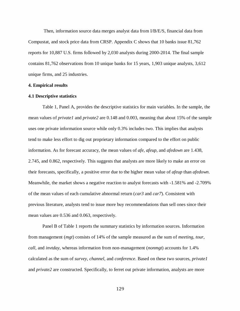
129

Then, information source data merges analyst data from I/B/E/S, financial data from

Compustat, and stock price data from CRSP. Appendix C shows that 10 banks issue 81,762

reports for 10,887 U.S. firms followed by 2,030 analysts during 2000-2014. The final sample

contains 81,762 observations from 10 unique banks for 15 years, 1,903 unique analysts, 3,612

unique firms, and 25 industries.

4. Empirical results

4.1 Descriptive statistics

Table 1, Panel A, provides the descriptive statistics for main variables. In the sample, the

mean values of private1 and private2 are 0.148 and 0.003, meaning that about 15% of the sample

uses one private information source while only 0.3% includes two. This implies that analysts

tend to make less effort to dig out proprietary information compared to the effort on public

information. As for forecast accuracy, the mean values of afe, afeup, and afedown are 1.438,

2.745, and 0.862, respectively. This suggests that analysts are more likely to make an error on

their forecasts, specifically, a positive error due to the higher mean value of afeup than afedown.

Meanwhile, the market shows a negative reaction to analyst forecasts with -1.581% and -2.709%

of the mean values of each cumulative abnormal return (car3 and car7). Consistent with

previous literature, analysts tend to issue more buy recommendations than sell ones since their

mean values are 0.536 and 0.063, respectively.

Panel B of Table 1 reports the summary statistics by information sources. Information

from management (mgt) consists of 14% of the sample measured as the sum of meeting, tour,

call, and invtday, whereas information from non-management (nonmgt) accounts for 1.4%

calculated as the sum of survey, channel, and conference. Based on these two sources, private1

and private2 are constructed. Specifically, to ferret out private information, analysts are more

130

likely to attend an investor/analyst day with the mean value of 0.082 (i.e., 8.2% of the sample)

followed by a personal meeting with management (0.028), conference call (0.023), and site tour

(0.007). On the other hand, 78% of the report sample describes earnings announcement (ea)

publicly made by a firm, suggesting what most high-paid analysts do, i.e., processing public

information. The overall average value of all information sources is 1.185 (i.e., 119% of the

sample) since some of them are duplicated.

Panel A of Table 2 shows the sample distribution by year during 2000-2014.33 Over the

years, analysts generally use more private information sources for forecasts, whereas forecast

error gradually decreases. This increases the informativeness of such forecasts, resulting in a

stronger market reaction to them. Specifically, the mean value of absolute forecast error (afe)

increases during two financial crisis periods (i.e., 2001, and 2007-2009).34 Following the crises

when they tend to conservative to incorporate new information, analysts make more efforts by

collecting/using more private information for forecasts, resulting in less afe compared to 1.473 of

its mean value. This suggests that research efforts to discover private information are likely to

reduce forecast error.

Panel B of Table 2 summarizes the distribution of the sample by 24 industry groups in

terms of the Global Industry Classification Standard (GICS) codes. Based on the sum of private1

and private2, Pharmaceuticals, Biotechnology & Life Sciences, Insurance, and Technology

Hardware & Equipment are top three industries which analysts collect information through

private channels rather than depend on a firm’s public information. These industries tend to hold

more investor/analyst days and industry conferences. Meanwhile, Banks has the highest forecast

33 The sample period starts on January 18, 2000 and ends on November 12, 2014. Thus, there are fewer observations

in both 2000 and 2014. 34 The National Bureau of Economic Research (NBER) reports that the recession periods are from March 15th, 2001

to November 15th, 2001, and from December 15th, 2007 to June 15th, 2009.

131

error with 2.735 of its mean value, followed by Real Estate with 2.643 and Telecommunication

Services with 2.623. Since they are likely to have more intangible assets, it is more difficult for

analysts to make accurate forecasts. Graphically, Panel B of Table 2 shows that the number of

private information sources is negatively related to the level of forecast error, but positively

associated with the market reaction. This hints that forecasts with private information sources

prone to have a fewer forecast error which investors value.

Table 3 displays the Pearson correlation matrix. As expected, the levels of private

information sources (private1 and private2) are significantly and negatively correlated with

forecast error (afe), but positively correlated with the level measures of market reaction (car3

and car7). This suggests that the more private research efforts, the better forecast accuracy and

the stronger market reaction. As expected, the level measures of market reaction (car3 and car7)

and afe are significantly and negatively correlated. Both private1 and private2 are significantly

and positively related to the size of analysts’ employer (brsize) and covering firm (logmv) where

analysts can access to more private information channels. On the other hand, private1 and

private2 are negatively related to the measures of an analyst’s busyness (firm_covered and

industry_covered). This implies that when analysts are busier with more firms and industries to

cover, they tend to count on more public information sources and thus make fewer efforts to find

private information sources.

Table 4, Panel A, shows how the sample is distributed by the levels of private

information sources. As in the descriptive statistics, private1 and private2 account for 15.13%

combined. Panel B of Table 4 summarizes that analysts overwhelmingly secure 1 private

information (private1) through management sources (mgt) among which investor/analyst day

(invstday) accounts for over 50%, followed by a personal meeting with management (meeting)

132

and a conference call (call). As for non-management sources (nonmgt), an industry contact such

as an industry conference (conference) is the number one source for private information. When it

comes to private2, analysts use two sources from management to discover proprietary

information over 61% of the time. Panel C of Table 4 explains the two sources in detail of which

40% (96/241*100) consists of the combination of a personal management meeting and an

investor/analyst day.

4.2 Univariate test

Table 5, Panel A, displays the mean comparisons by private research effort levels. As the

effort level increases, the forecast error (afe) significantly decreases, suggesting initial evidence

that the more private information sources, the higher forecast accuracy. Accordingly, market

reaction also becomes stronger, especially, significantly from non-private information (private0)

to one (private1). Panel B of Table 5 shows that when analysts take advantage of single private

information (private1) to make forecasts, management sources are more useful to reduce forecast

error (afe).

Given that there is one more proprietary information to use (private2), more accurate and

informative forecasts can be made by the combination of management and non-management

sources compared to that of management sources themselves. Overall, the univariate comparison

suggests that more private research efforts improve forecast quality in terms of its accuracy and

thus drives a stronger market reaction.

4.3 Main regression analyses

All previous analyses indicate that the number of private information sources has a

negative (positive) relationship with the level of forecast error (market reaction). In this section, I

investigate the multiple regression model specified in Section 3 with/without control variables.

133

4.3.1 Analysts’ private research effort and earnings forecast accuracy

Table 6 reports the linear regression results of the effect of the number of private

information sources on analysts’ earnings forecast error. First, coefficients on private1 are not

significant across the models since a single public information source influences forecast error as

much as a single private source does, implying that public sources are also useful for analyst

performance. In Columns (1) and (2), however, private2 is significantly and negatively related to

afe, suggesting that forecasts made with additional private information source are less (more)

likely to have forecast error (accuracy). The statistical significance of its coefficient is stronger

even with control variables than without. This is consistent with the first hypothesis.

Then, the question is which forecast error a private information source can reduce, i.e.,

positive or negative forecast error. Columns (3) to (6) have the answer, showing that proprietary

information is more likely to decrease positive forecast error (afeup) than its counterpart

(afedown), especially with control variables.

The results show that all coefficients on private2 but those in the negative forecast

models are negative and significant at p<0.01 while that of private1 is not. More importantly, the

results indicate the economic impact of an additional private information source. For instance,

the model 2 of Table 6 finds that the magnitude of private2 is large (i.e., -0.488 of its

coefficient), meaning that additional private information reduces forecast error (afe) by almost a

half dollar. Alternatively, a one standard deviation increase in private2 is associated with a

decrease of 0.03 in afe. This effect is economically significant as it represents a 2.1% decrease

below the mean afe of 1.438. This also leads to a 1% standard deviation reduction in afe, all else

equal. The results suggest that the negative association between private information and forecast

134

error is statistically and economically significant. Overall, Table 6 confirms the prediction that

extra information from private sources increases (reduces) forecast accuracy (error).

Meanwhile, all firm-specific variables except for the number of analyst following

(lognanalyst) are statistically significant at the 1% level across the models. Specifically, forecast

error (afe) is negatively related with a size (logmv), market value (mb), profitability (roa) and

institutional investor’s holding (iholding) of a firm, but positively related to its risk such as

previous return volatility (retstd12) and negative earnings experience (loss). On the other hand,

all analyst-specific variables are not significant except for horizon which is positively related to

afe, suggesting that with a longer horizon (i.e., more days to fiscal year-end from a forecast

date), analysts tend to have more forecast errors since they have less accurate information and

thus make more assumptions on the forecasts.

4.3.2 Analysts’ private research effort and market reaction to stock recommendations

In order to determine the usefulness of private information sources, I analyze their

information content. Given that analysts issue more accurate forecasts using private information

sources, I expect a stronger market reaction to stock recommendations issued by them. To test

the relative importance of information sources on market reaction to recommendations, I

estimate the market reaction model in Equation 2. Specifically, I regress car3 (or car7) on the

levels of private sources (private1 and private2), controlling for the characteristics of

recommendations (buy, sell, and ∆recom), forecast error (afe) and all variables from

specifications of Table 6.

Table 7 shows that across the models, all proxies (private1 and private2) for the number

of private information sources are significantly and positively related to those (car3 and car7) for

cumulative abnormal return. Specifically, all coefficients on private1 are positive and significant

135

at p<0.01. All coefficients on private2 except for that in Column (1) are at p<0.05, suggesting

their statistical significance. However, the magnitude of private2 is almost twice greater than

private1 because all coefficients on the former are bigger than those on the latter across the

models, suggesting that market reaction is higher for stock recommendations issued by analysts

with higher private research efforts. In other words, one unit increase in private2 (i.e., an

increase of additional two private information) will increase cumulative abnormal returns by 1%.

More specifically, in Column (2), a one standard deviation increase in private2 increases a

standard deviation in car3 by 1% compared to that in private1 by 0.26%. Overall, the results

suggest that in addition to its statistical significance, private information source have an

economic impact on stock returns if I fix all the other variables at a fixed value, implying that

investors value the hard work analysts make for forecasts, and recognize their accuracy and

informativeness.35

Consistent with previous literature on analysts’ signals, cumulative abnormal returns

(car3 and car7) are positively associated with both a buy recommendation (buy) and its change

(∆recom), whereas negatively with a sell recommendation (sell). As for control variables specific

to analysts, they also have a positive relationship with brokerage size (brsize), industry

experience (industryexp), and the number of days from a forecast date to fiscal year-end

(horizon). On the other hand, they are negatively correlated with forecast error (afe), and firm

experience (firmexp). In terms of firm-specific control variables, cumulative abnormal returns

are negatively related with a firm’s size (logmv), leverage (leverage), past return volatility

35 I run separate regressions on buy and sell recommendations due to asymmetric market reaction after controlling

for the change of recommendations along with all variables form Table 6. The untabulated reports show the similar

results with those of Table 7.

136

(retstd12), and the number of analyst following (lognanalyst). Only the market value (mb) of a

firm is positively associated with cumulative abnormal returns.

4.3.3 Analysts’ earnings forecast accuracy and market reaction based on the type of private

information sources

In the descriptive statistics section, Panel C of Table 4 displays the distribution of the

level of private research efforts equal to 2 (private2) based on two main information sources, i.e.,

management (mgt) and non-management (nonmgt) sources. In the main regression analysis

section, Table 6 and 7 show the negative effect of private2 on forecast error (afe) and its positive

consequence on market reaction (car3 and car7), respectively. In this section, I investigate the

impact of private2 in terms of two information sources in both the forecast error model and the

market reaction model since private1 is not significant in the first model.

Table 8, Panel A, includes two variables for two private information (private2), i.e.,

private2single (private2mix) equal to 1 if analysts collect information from two (at least one)

management (non-management) sources, and 0 otherwise. In Panel C of Table 4, there are two

types of the combination for private2mix, i.e., one from one management and one non-

management source (e.g., an investor/analyst day and an industry conference) and another from

two non-management sources (e.g., a channel check and an industry conference). Table 8 does

not include the latter since there is only one combination of two non-management sources.

Specifically, Panel A of Table 8 shows that all the coefficients on private2mix are negative and

significant at the 1% level except for that in model 3 at the 5% level. This implies that forecasts

made based on two private information for which analysts acquire from both one management

source and one non-management source are more likely to have the least errors across the source

types. This also suggests that private information from a supply chain analysis (channel) or an

137

industry meeting (conference) is as useful as management-source information for analysts to

produce more accurate forecasts since the information contains a big picture of the firm analysts

follow, which helps them better understand the firm. Meanwhile, the association between afe and

control variables is similar to that in Table 6.

Panel B of Table 8 reports that almost all types of source variables except for

private2single are positive and significant at p<0.01. This indicates that private information is

informative for investors to make their investment decisions. Especially, additional proprietary

information from each of management and non-management sources contributes to higher

cumulative abnormal returns (car3 and car7) since the coefficients on private2mix are bigger

than any other ones. As for control variables, their signs are similar to those in Table 7.

Collectively, private information from both management and non-management sources is

useful for analysts because they are able to make more accurate forecasts. Such information is

also beneficial for investors to make a better judgement on their investment.

5. Robustness checks

In this section, I implement a battery of robustness tests on the results of Table 6 and 7.

The results are robust to different specifications using a different measure of forecast errors as

well as more control variables, and to the mean value regression of forecast errors.

5.1 Additional control variables (i.e., Form 10-K readability and analyst connection), and a

new forecast error measure

First, I replicate the results of Table 6 and 7 using the readability level of annual reports

(i.e., Form 10-Ks) (readability) and analysts’ relationship with the covered firm (connection) as

additional control variables which may affect forecast accuracy and market reaction.

Specifically, referring to previous research (De Franco, Hope, Vyas, and Zhou, 2015), I first

138

create a measure of readability levels of 10-Ks (readability) defined as aggregate readability

measure of Gunning-Fog Unreadability Index, Kincaid Flesch-Kincaid Grade Level index,

Flesch Reading Ease Score, and Smog Readability Index by multiplying the first two and the last

one by negative one to ensure that all components are increasing in readability, ranking each

component into percentiles from 1 to 100, and then taking the average across the four

components.36 Interpretation of the 10-K readability measure is that the higher readability, the

easier it is to read.

On the other hand, analysts may have various relationships with the firm they follow, i.e.,

a client, investment banking, and/or brokerage; they even can own a share of the firm. These

connections with the covered firm might influence analysts’ ability on forecasts and thus the

informativeness of forecasts. Accordingly, I create a variable named connection equal to 1 when

analysts have any types of these relationships with the covered firm, and 0 otherwise.

Instead of forecast error divided by average monthly stock price in equation 1, I use

actual earnings as a scaler, create a variable named afeact, and include in Columns (2), (5), and

(6) of Table 9 for comparison with Columns (1), (3), and (4) of Table 9.

Consistent with the results of Table 6 and 7, private2 is significantly negatively related

with both afe and afeact, and has a significantly positive association with car3 and car7. This

suggests that more private information sources improve analyst performance in terms of forecast

accuracy and thus, strengthen investors’ belief in the forecast. The directions of the control

variable are similar to those in Table 6 and 7.

36 Fog index refers to Gunning-Fog Unreadability Index, calculated as -1 x ((0.4 x words per sentence) + (100 x

complex words per word)). Kincaid Flesch-Kincaid Grade Level index is calculated as -1 x ((0.39 x words per

sentence) + (11.8 x syllables per word) – 15.59)). Flesch Reading Ease Score is measured as 206.835 – (1.015 x

words per sentence) – (84.6 x syllables per word). Smog Readability Index is calculated as -1 * (1.043 x sqrt (#

complex words x 30/# sentences) + 3.1291).

139

5.2 Mean value regressions of earnings forecast error

To eliminate the undesirable effect from extreme values of variables, I repeat the models

in Table 6 using the mean values of all variables except for private information source variables.

This process reduces the number of observations to slightly more than 1,700 on average. Table

11 shows the results with a bank fixed effect included and standard errors cluster-adjusted at a

bank level. Consistent with the findings of Table 6, more private research efforts (private2)

significantly decrease average forecast errors across the models.

Meanwhile, the untabulated results of mean value regressions show that market reaction

is consistent with that of Table 7.

6. Change analyses

So far, the findings show the robust association of private information with forecast

accuracy and market reaction. Next, based on the panel data, I can implement time-series tests to

find a possible causal relationship by investigating a directional impact; and to eliminate a fixed

effect. Specifically, causality may be established by dealing with reverse causality by self-

selection since analysts making forecasts with more errors are more likely to exert more private

research efforts. To address this endogeneity issue, I conduct a change analysis on both forecast

error and market reaction models. Specifically, I examine whether an increase in the number of

private information sources (privateincrease) in analyst forecasts are negatively associated with

changes in forecast error (afechg) and positively related to changes in cumulative abnormal

returns (car3chg and car7chg). Table 9 shows the results. In Columns (1) and (2) of Table 10,

increase in proprietary information sources (privateincrease) is significantly negatively related to

change in forecast error (afechg) at p<0.01, consistent with the findings for the level of private

information sources in Table 6 and 9.

140

I further examine the change in market reaction in Columns (3) to (6) of Table 10.

Coefficients on an increase in input levels are positive and significant at the 1% level, suggesting

the informativeness of additional private information, in line with the results in Table 7 and 9.

In general, the results of the change analyses imply that more proprietary information

from a private source may cause decrease in forecast errors and increase in market reaction.

7. Analysts’ private research effort vs. information advantage

I find that analysts with more private research efforts tend to make superior forecasts. In

other words, forecasts by these analysts have better quality in terms of accuracy which investors

favorably react to. However, according to an analyst black box survey paper (Brown, Call, and

Clement, 2015), analysts, especially, those who work at big brokerage firms, are more likely to

make better forecasts because of information advantage from private phone calls with

management. Therefore, it is crucial to investigate whether analysts’ private research efforts also

produce better forecasts.

For this task, I construct a sample by identifying analysts who do not make any effort on

private information sources in the first place, but make efforts afterward. Specifically, if

forecasts from these analysts with high efforts (high_type) have less error and a stronger market

reaction, then the research is consistent with analyst effort hypothesis. Otherwise, it is based on

analyst information advantage explanation. high_type is an indicator variable equal to 1 if private

research efforts are greater than 0 after no effort in the first place.

Columns (1) and (2) of Table 12 show that high_type and afe are negatively related at

p<0.05, suggesting that generally, high efforts on additional private information is instrumental

for analysts to make more accurate forecasts. Based on a comparison of Columns (3) and (4)

141

with Columns (5) and (6), high effort analysts are less likely to make negative forecasts than

positive ones. Control variables have a similar pattern with that in Table 6.

Consequently, the results of Table 12 support the effort hypothesis in Section 2,

providing a new perspective on analyst performance, especially, in terms of forecast accuracy.

Meanwhile, market reaction is also investigated, and its untabulated results show a

similar pattern with the market reaction of Table 7.

8. Determinants of analysts’ private research efforts

To identify the determinants of the level of proprietary information (private) analysts

discover from private sources, I regress a categorical variable, private, on analyst and firm

characteristics using ordered logit regression. The specification includes all independent

variables of Panel A of Table 9. In addition, I add more analyst-specific variables: analyst gender

(female) equal to 1 if the analyst is a female, and 0 otherwise; analyst location (foreign) equal to

1 if analyst resides outside of U.S., and 0 otherwise; analyst education level (graduate) equal to 1

if analyst holds a graduate degree, and 0 otherwise. I also create one more firm-specific variable,

turnover, calculated as 100 times the number of shares traded for a firm deflated by the total

number of common shares outstanding in year t. Model 1 and 2 of Table 13 do not include any

fixed effect without any clustering, whereas Model 3 and 4 contain all three fixed effects with

firm clustering.

The results of Table 13 show that analysts from a large brokerage house (brsize), with

more days to fiscal year-end from forecast date (horizon), with a graduate degree (graduate), or

with more connections with the firm they follow (connection) are more likely to make more

efforts to dig out private sources for more proprietary information. On the contrary, analysts with

more firms to cover (firm_covered) or those residing in non-U.S. countries (foreign) tend to exert

142

less private research effort because they are busy or have fewer information sources outside of

the U.S..

Table 13 also finds that analysts following a firm in a bigger size (logmv), with higher

standard deviation in previous returns (retstd12), or with more percentage of institutional

investors (iholding) are more likely to be more efforts to secure more private information. On the

other hand, analysts covering a firm with higher profitably (roa) or less readable 10-Ks

(readability) are less likely to make an effort on the detective work to find private information

sources.

9. Conclusion and Future Direction

There is a little literature on what analysts do, that is, how they produce their research

reports. Put differently, we know little about what information source analysts use to make

forecasts, and which information source is more valuable. As an information intermediary,

analysts access to private and/or public information source of a firm to make forecasts for

investors. Previous studies consistently find a higher accuracy of forecasts made based on private

information sources. Two sources, however, might equally useful for analysts to reduce forecast

error. In terms of value relevance, prior research finds mixed evidence. This is because prior

studies cannot precisely identify private and public information sources.

To address the identification issue, the research implements advanced textual analysis

using a regular expression for a pattern search on a headline of 81,762 analyst reports during

2000-2014. The study finds that there is no significant difference between single private and

single public information source in terms of analysts’ earnings forecast error (or accuracy), but

an additional proprietary information source might cause a decrease (increase) in forecast errors

(accuracy). Given that an additional private source requires more efforts to get on the part of

143

analysts (even when they do not have an information advantage), investors highly appreciate the

efforts by reacting stronger to a recommendation issued based on forecasts containing the private

information. This new perspective makes the study to be differentiated from previous literature

supporting analysts’ information advantage hypothesis.

Further analysis shows that the combination of two private information from each of

management and non-management sources is more likely to reduce more forecast errors and to

stronger market reaction than any other combination. Additional cross-sectional analyses

investigate the determinants of the level of private information sources based on a variety of

analyst and firm characteristics, and find most of them to be significant explanatory variables.

The most significant contribution the research makes to the literature is developing a

novel measure to accurately identify information sources in analyst reports which previous

studies cannot. Specifically, the study employs advanced textual analysis known as a regular

expression for a pattern search on a headline of analyst reports. This algorithm allows the

research to explain a possible market reaction channel, i.e., forecast accuracy.

Institutional Investor (II) magazine selects the best research analysts every year. 37

However, it is a reasonable concern that their methodology might be highly subjective because

the weighting of votes is heavily skewed toward institutions with the most assets under

management and those that pay Wall Street the most commissions and thus, selected analysts

have an information advantage. Using a sample of the best analysts of the year from the

magazine, future research investigates whether these All-Star analysts make as much effort to

discover private information sources to live up to their reputation and compensation. If this is

37 The All-America team is selected by a survey of research directors and chief investment officers of major asset

management firms, including the largest U.S. money managers and significant U.S., European and Asian

institutional investors. Clients get into the mix and analysts themselves are asked to assess their peers. See the link

(https://www.institutionalinvestor.com/research/7394/Methodology) for more detail.

144

empirically true, then they deserve to be a star since they work hard rather than have information

advantage in access to proprietary sources.

It is important to note that my results might be subject to limitations. For example, while

I conduct textual analysis based on headlines and the first 50 words of analyst reports, I

acknowledge that such a decision can potentially lead to the issue of an incomplete sample. To

reduce this concern, I validate the accuracy of the keyword identification by applying the textual

analysis to 20 randomly selected analyst reports with full length. My result indicated that

although I am able to identify more matches using the entire report instead of focusing on only

the headline and top 50 words, the correlation of the keywords identified using my current

approach and the full report is close to 70%. This finding suggests that although the accuracy of

keyword identification can indeed increase using the full report, the focus on the headline and

first 50 words can represent a reasonable tradeoff between effort and efficiency given the large

number of analyst reports.

145

References

Asquith, P., Mikhail, M., and Au, A., 2005. Information content of equity analyst reports.

Journal of Financial Economics 75, 245-282.

Beyer A., Cohen D., Lys T., and Walther B., 2010. The financial reporting environment: Review

of the recent literature. Journal of Accounting and Economics 50, 296–343.

Bradshaw M., 2011. Analysts’ forecasts: What do we know after decades of work? Working

paper, Boston College, Chestnut Hill, MA.

Brown, L., Call, A., and Clement, M., 2015. Inside the “Black Box” of Sell-Side Financial

Analysts. Journal of Accounting Research 53, 1–47.

Bushee, B., Matsumoto, D., Miller, G., 2003. Open versus closed conference calls: the

determinants and effects of broadening access to disclosure. Journal of Accounting and

Economics 34, 149–180.

Chen, X., Cheng, Q., and Lo, K., 2010. On the relationship between analyst reports and

corporate disclosures: Exploring the roles of information discovery and interpretation.

Journal of Accounting and Economics 49, 206–226.

Clement, M., 1999. Analyst Forecast Accuracy: Do Ability, Resources, and Portfolio

Complexity Matter?. Journal of Accounting and Economics 27, 285–303.

Daniel, N., Lee, S., and Naveen, L., 2015. Information discovery by analysts. Working paper.

De Franco, G., Hope, O.K., Vyas, D., and Zhou, Y. 2015. Analyst report readability.

Contemporary Accounting Research 32, 76–104.

Hong, H., and Kubik, J. D., 2003. Analyzing the analysts: Career concerns and biased earnings

forecasts. The Journal of Finance 58, 313–51.

Huang, A., Lehavy, R., Zang, A., and Zheng, R., 2017. Analyst Information Discovery and

Interpretation Roles: A Topic Modeling Approach. Management science 63, 1–23

Ivkovic, Z. and Jegadeesh, N., 2004. The timing and value of forecast and recommendation

revisions. Journal of Financial Economics 73, 433-463.

Livnat, J., and Zhang, Y., 2012. Information interpretation or information discovery: Which role

of analysts do investors value more?. Review of Accounting Studies 17, 612-641.

Lo, K., 2012. What do analysts do? Discussion of “Information interpretation or information

discovery: which role of analysts do investors value more?”. Review of Accounting Studies

17, 642-648.

Loh, R. and Mian, G., 2006. Do accurate earnings forecasts facilitate superior investment

recommendations? Journal of Financial Economics 80, 455-483.

Ramnath, S., Rock, S., and Shane, P., 2008. The financial analyst forecast literature: A taxonomy

with suggestions for future research. International Journal of Forecasting 24, 34–75.

Richardson, S., Teoh, S., and Wysocki, P., 2004. The Walk-down to Beatable Analyst Forecasts:

The Role of Equity Issuance and Insider Trading Incentives. Contemporary Accounting

Research, 21, 885–924.

Rubin, A., Segal, B., and Segal, D., 2017. The interpretation of unanticipated news arrival and

analysts’ skill. Journal of Financial and Quantitative Analysis 52, 1491-1518.

Rubin, A., and Segal, D., 2016. The Discovery Role of Analysts. Working paper.

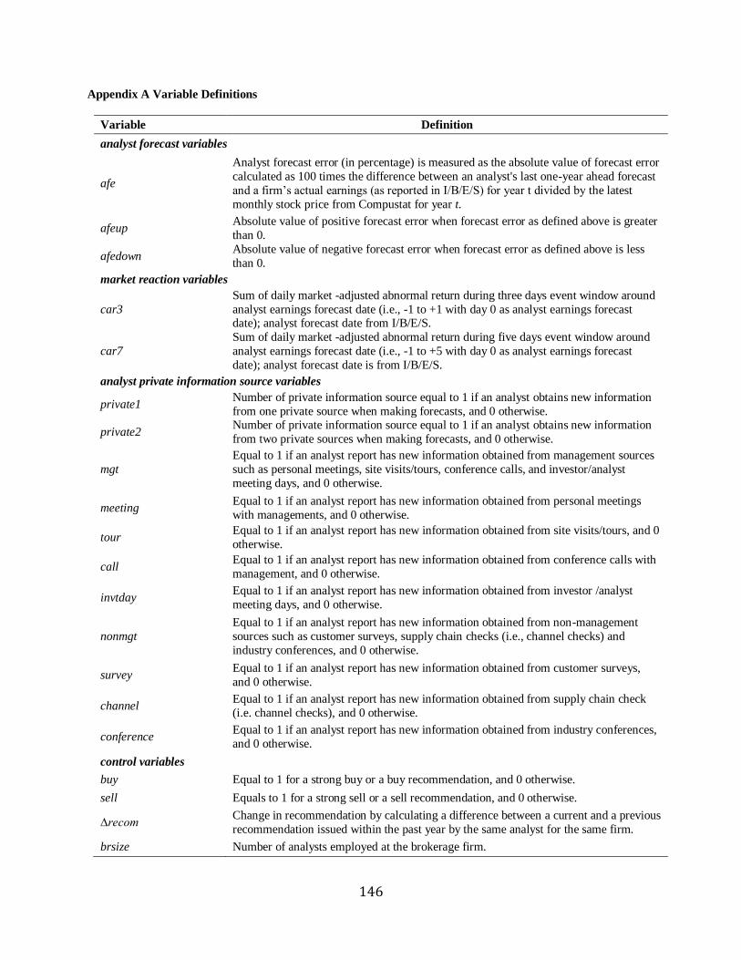
146

Appendix A Variable Definitions

Variable Definition

analyst forecast variables

afe

Analyst forecast error (in percentage) is measured as the absolute value of forecast error

calculated as 100 times the difference between an analyst's last one-year ahead forecast

and a firm’s actual earnings (as reported in I/B/E/S) for year t divided by the latest

monthly stock price from Compustat for year t.

afeup Absolute value of positive forecast error when forecast error as defined above is greater

than 0.

afedown Absolute value of negative forecast error when forecast error as defined above is less

than 0.

market reaction variables

car3

Sum of daily market -adjusted abnormal return during three days event window around

analyst earnings forecast date (i.e., -1 to +1 with day 0 as analyst earnings forecast date); analyst forecast date from I/B/E/S.

car7

Sum of daily market -adjusted abnormal return during five days event window around

analyst earnings forecast date (i.e., -1 to +5 with day 0 as analyst earnings forecast

date); analyst forecast date is from I/B/E/S.

analyst private information source variables

private1 Number of private information source equal to 1 if an analyst obtains new information

from one private source when making forecasts, and 0 otherwise.

private2 Number of private information source equal to 1 if an analyst obtains new information

from two private sources when making forecasts, and 0 otherwise.

mgt

Equal to 1 if an analyst report has new information obtained from management sources

such as personal meetings, site visits/tours, conference calls, and investor/analyst

meeting days, and 0 otherwise.

meeting Equal to 1 if an analyst report has new information obtained from personal meetings

with managements, and 0 otherwise.

tour Equal to 1 if an analyst report has new information obtained from site visits/tours, and 0

otherwise.

call Equal to 1 if an analyst report has new information obtained from conference calls with

management, and 0 otherwise.

invtday Equal to 1 if an analyst report has new information obtained from investor /analyst

meeting days, and 0 otherwise.

nonmgt

Equal to 1 if an analyst report has new information obtained from non-management

sources such as customer surveys, supply chain checks (i.e., channel checks) and

industry conferences, and 0 otherwise.

survey Equal to 1 if an analyst report has new information obtained from customer surveys,

and 0 otherwise.

channel Equal to 1 if an analyst report has new information obtained from supply chain check

(i.e. channel checks), and 0 otherwise.

conference Equal to 1 if an analyst report has new information obtained from industry conferences,

and 0 otherwise.

control variables

buy Equal to 1 for a strong buy or a buy recommendation, and 0 otherwise.

sell Equals to 1 for a strong sell or a sell recommendation, and 0 otherwise.

∆recom Change in recommendation by calculating a difference between a current and a previous

recommendation issued within the past year by the same analyst for the same firm.

brsize Number of analysts employed at the brokerage firm.

147

firmexp Firm experience, calculated as the number of years for which an analyst supplies a

forecast for the firm.

industryexp Industry experience, measured as the number of years since an analyst covered the

firm’s industry.

firm_covered Number of firms covered is defined as the number of firms an analyst follows.

industry_covered Number of industries covered is calculated as the number of industries an analyst

follows.

horizon Number of days between a forecast date and a forecast period end date (i.e., a fiscal

year-end date).

logmv Natural logarithm of firm's market capitalization in U.S. $ million, i.e., common shares outstanding multiplied by the fiscal year-end price.

mb Ratio of market value to book value of a firm at year-end.

roa Ratio of income before extraordinary items to total assets at the end of year t.

leverage Total liabilities divided by total assets at year-end

retstd12 Standard deviation of daily stock return for a firm during 12 months prior to an analyst

forecast date.

loss Equal to 1 if a firm has a negative earnings during three fiscal years prior to an analyst forecast, and 0 otherwise

lognanalyst Natural logarithm of the number of analysts following the firm in the previous year.

iholding

Institutional holding is measured as the total number of shares held by institutions

divided by shares outstanding at the end of the same quarter. The percentage holdings

of institutional investors are 0 if no institutional investor reports positive holdings for a

firm-quarter.

readability

Aggregate annual report (i.e., Form 10-K) readability measure of Fog, Flesch-Kincaid,

Flesch Reading Ease, and Smog Readability Index by multiplying the first two and the

last one by negative one to ensure that all components are increasing in readability, ranking each component into percentiles from 1 to 100, and then taking the average

across the four components. The higher readability, the easier to read.

connection Equal to 1 for the analyst has any of client, investment, brokerage, and/or ownership

relationship with the covered firm, and 0 otherwise.

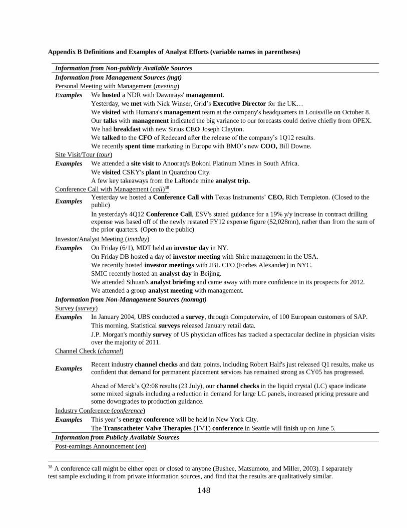
148

Appendix B Definitions and Examples of Analyst Efforts (variable names in parentheses)

Information from Non-publicly Available Sources

Information from Management Sources (mgt)

Personal Meeting with Management (meeting)

Examples We hosted a NDR with Dawnrays' management.

Yesterday, we met with Nick Winser, Grid’s Executive Director for the UK…

We visited with Humana's management team at the company's headquarters in Louisville on October 8.

Our talks with management indicated the big variance to our forecasts could derive chiefly from OPEX.

We had breakfast with new Sirius CEO Joseph Clayton.

We talked to the CFO of Redecard after the release of the company’s 1Q12 results.

We recently spent time marketing in Europe with BMO’s new COO, Bill Downe.

Site Visit/Tour (tour)

Examples We attended a site visit to Anooraq's Bokoni Platinum Mines in South Africa.

We visited CSKY's plant in Quanzhou City.

A few key takeaways from the LaRonde mine analyst trip.

Conference Call with Management (call)38

Examples Yesterday we hosted a Conference Call with Texas Instruments’ CEO, Rich Templeton. (Closed to the

public)

In yesterday's 4Q12 Conference Call, ESV's stated guidance for a 19% y/y increase in contract drilling expense was based off of the newly restated FY12 expense figure ($2,028mn), rather than from the sum of

the prior quarters. (Open to the public)

Investor/Analyst Meeting (invtday)

Examples On Friday (6/1), MDT held an investor day in NY.

On Friday DB hosted a day of investor meeting with Shire management in the USA.

We recently hosted investor meetings with JBL CFO (Forbes Alexander) in NYC.

SMIC recently hosted an analyst day in Beijing.

We attended Sihuan's analyst briefing and came away with more confidence in its prospects for 2012.

We attended a group analyst meeting with management.

Information from Non-Management Sources (nonmgt)

Survey (survey)

Examples In January 2004, UBS conducted a survey, through Computerwire, of 100 European customers of SAP.

This morning, Statistical surveys released January retail data.

J.P. Morgan's monthly survey of US physician offices has tracked a spectacular decline in physician visits

over the majority of 2011.

Channel Check (channel)

Examples Recent industry channel checks and data points, including Robert Half's just released Q1 results, make us

confident that demand for permanent placement services has remained strong as CY05 has progressed.

Ahead of Merck’s Q2:08 results (23 July), our channel checks in the liquid crystal (LC) space indicate

some mixed signals including a reduction in demand for large LC panels, increased pricing pressure and

some downgrades to production guidance.

Industry Conference (conference)

Examples This year’s energy conference will be held in New York City.

The Transcatheter Valve Therapies (TVT) conference in Seattle will finish up on June 5.

Information from Publicly Available Sources

Post-earnings Announcement (ea)

38 A conference call might be either open or closed to anyone (Bushee, Matsumoto, and Miller, 2003). I separately

test sample excluding it from private information sources, and find that the results are qualitatively similar.

149

Examples VMED has reported Q4 results.

Mitsui Fudosan announced 3Q FY2012 results after the close of trading on February 6.

3QFY12 results beat expectations.

EPS were in-line with our forecast.

Ipsos guided that FY 2003 results (due March 23 ) will show a further rise in operating margin.

In yesterday's 4Q12 conference call, ESV's stated guidance for a 19% y/y increase in contract drilling expense was based off of the newly restated FY12 expense figure ($2,028mn), rather than from the sum of

the prior quarters.

Pre-earnings Announcement (preea)

Examples We forecast revenue will grow 14% annually in both 2012 and 2013.

We expect F2Q results to be good enough.

We preview SIP ahead of the release of its FY12 result on 22 March 2012.

Non-Earnings Announcement (nonea)

Examples We believe the resignation of Carly Fiorina as Chairman and CEO signals that the board is ready to take

more aggressive actions to create shareholder value.

Devon Energy Announces Merger with Santa Fe Snyder.

MFC announced a hostile offer to acquire the CL shares.

GMR announced that it initiates a cash dividend policy and plans to declare its initial dividend following

the first quarter earnings results.

We initiate coverage of MCE with an Overweight (V) rating.

A tentative legal settlement reached earlier this month in U S District Court in Boston.

Gluskin Sheff Associates raised million for selling shareholders in an initial public offering (IPO) that

closed May.

In the last two weeks we have seen two major developments in US power emissions regulation.

In Nov., EDU launched a new product.

Renesas officially announced details of its restructuring plan including cutting its workforce by about

completely outsourcing mass production of advanced process technology products to overseas foundries.

VRTS shares are down over the last trading sessions largely attributable to concerns that a slowdown at

SUNW could have a material impact on VRTS's business in coming quarters.

This is a significant new customer win for MONI.

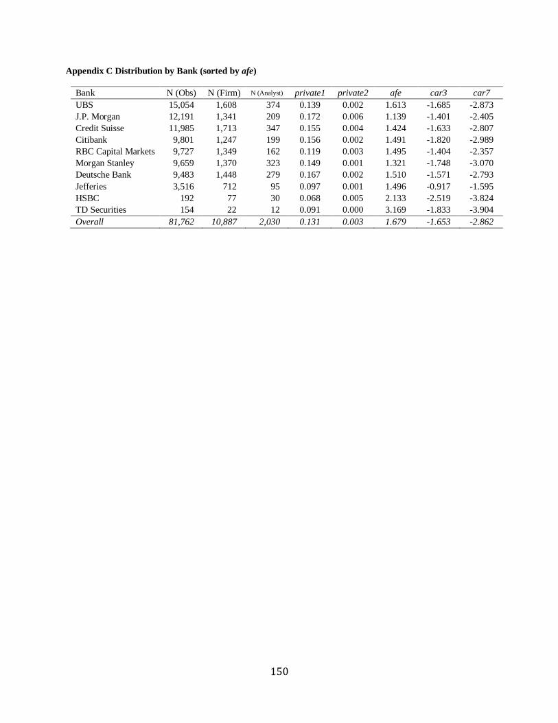
150

Appendix C Distribution by Bank (sorted by afe)

Bank N (Obs) N (Firm) N (Analyst) private1 private2 afe car3 car7

UBS 15,054 1,608 374 0.139 0.002 1.613 -1.685 -2.873

J.P. Morgan 12,191 1,341 209 0.172 0.006 1.139 -1.401 -2.405

Credit Suisse 11,985 1,713 347 0.155 0.004 1.424 -1.633 -2.807

Citibank 9,801 1,247 199 0.156 0.002 1.491 -1.820 -2.989

RBC Capital Markets 9,727 1,349 162 0.119 0.003 1.495 -1.404 -2.357

Morgan Stanley 9,659 1,370 323 0.149 0.001 1.321 -1.748 -3.070

Deutsche Bank 9,483 1,448 279 0.167 0.002 1.510 -1.571 -2.793

Jefferies 3,516 712 95 0.097 0.001 1.496 -0.917 -1.595

HSBC 192 77 30 0.068 0.005 2.133 -2.519 -3.824

TD Securities 154 22 12 0.091 0.000 3.169 -1.833 -3.904

Overall 81,762 10,887 2,030 0.131 0.003 1.679 -1.653 -2.862

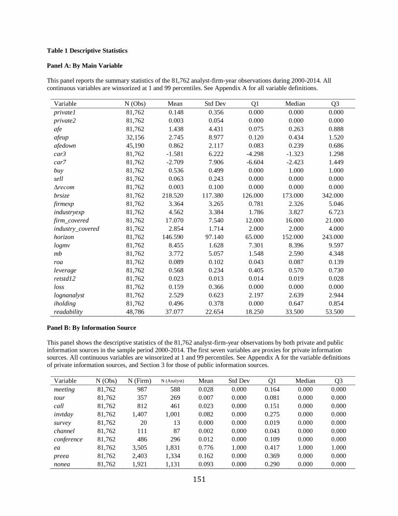
151

Table 1 Descriptive Statistics

Panel A: By Main Variable

This panel reports the summary statistics of the 81,762 analyst-firm-year observations during 2000-2014. All

continuous variables are winsorized at 1 and 99 percentiles. See Appendix A for all variable definitions.

Variable N (Obs) Mean Std Dev Q1 Median Q3

private1 81,762 0.148 0.356 0.000 0.000 0.000

private2 81,762 0.003 0.054 0.000 0.000 0.000

afe 81,762 1.438 4.431 0.075 0.263 0.888

afeup 32,156 2.745 8.977 0.120 0.434 1.520

afedown 45,190 0.862 2.117 0.083 0.239 0.686

car3 81,762 -1.581 6.222 -4.298 -1.323 1.298

car7 81,762 -2.709 7.906 -6.604 -2.423 1.449

buy 81,762 0.536 0.499 0.000 1.000 1.000

sell 81,762 0.063 0.243 0.000 0.000 0.000

∆recom 81,762 0.003 0.100 0.000 0.000 0.000

brsize 81,762 218.520 117.380 126.000 173.000 342.000

firmexp 81,762 3.364 3.265 0.781 2.326 5.046

industryexp 81,762 4.562 3.384 1.786 3.827 6.723

firm_covered 81,762 17.070 7.540 12.000 16.000 21.000

industry_covered 81,762 2.854 1.714 2.000 2.000 4.000

horizon 81,762 146.590 97.140 65.000 152.000 243.000

logmv 81,762 8.455 1.628 7.301 8.396 9.597

mb 81,762 3.772 5.057 1.548 2.590 4.348

roa 81,762 0.089 0.102 0.043 0.087 0.139

leverage 81,762 0.568 0.234 0.405 0.570 0.730

retstd12 81,762 0.023 0.013 0.014 0.019 0.028

loss 81,762 0.159 0.366 0.000 0.000 0.000

lognanalyst 81,762 2.529 0.623 2.197 2.639 2.944

iholding 81,762 0.496 0.378 0.000 0.647 0.854

readability 48,786 37.077 22.654 18.250 33.500 53.500

Panel B: By Information Source

This panel shows the descriptive statistics of the 81,762 analyst-firm-year observations by both private and public

information sources in the sample period 2000-2014. The first seven variables are proxies for private information sources. All continuous variables are winsorized at 1 and 99 percentiles. See Appendix A for the variable definitions

of private information sources, and Section 3 for those of public information sources.

Variable N (Obs) N (Firm) N (Analyst) Mean Std Dev Q1 Median Q3

meeting 81,762 987 588 0.028 0.000 0.164 0.000 0.000

tour 81,762 357 269 0.007 0.000 0.081 0.000 0.000

call 81,762 812 461 0.023 0.000 0.151 0.000 0.000

invtday 81,762 1,407 1,001 0.082 0.000 0.275 0.000 0.000

survey 81,762 20 13 0.000 0.000 0.019 0.000 0.000

channel 81,762 111 87 0.002 0.000 0.043 0.000 0.000

conference 81,762 486 296 0.012 0.000 0.109 0.000 0.000

ea 81,762 3,505 1,831 0.776 1.000 0.417 1.000 1.000

preea 81,762 2,403 1,334 0.162 0.000 0.369 0.000 0.000

nonea 81,762 1,921 1,131 0.093 0.000 0.290 0.000 0.000

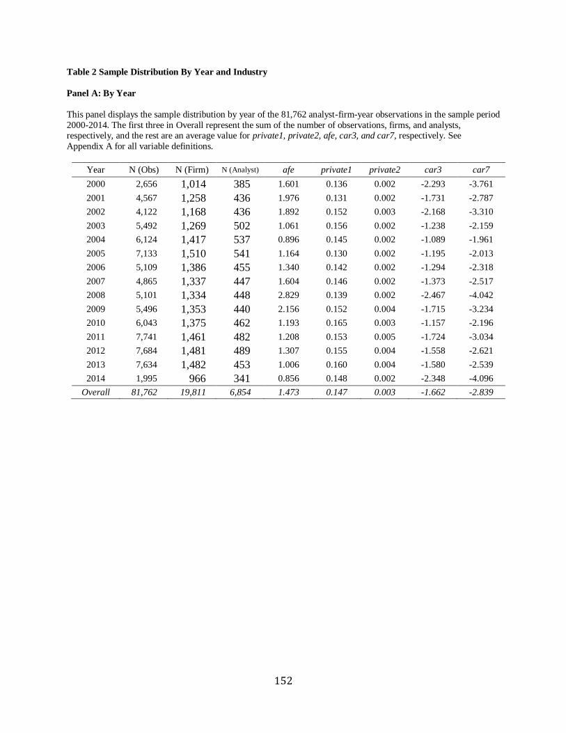
152

Table 2 Sample Distribution By Year and Industry

Panel A: By Year

This panel displays the sample distribution by year of the 81,762 analyst-firm-year observations in the sample period

2000-2014. The first three in Overall represent the sum of the number of observations, firms, and analysts, respectively, and the rest are an average value for private1, private2, afe, car3, and car7, respectively. See

Appendix A for all variable definitions.

Year N (Obs) N (Firm) N (Analyst) afe private1 private2 car3 car7

2000 2,656 1,014 385 1.601 0.136 0.002 -2.293 -3.761

2001 4,567 1,258 436 1.976 0.131 0.002 -1.731 -2.787

2002 4,122 1,168 436 1.892 0.152 0.003 -2.168 -3.310

2003 5,492 1,269 502 1.061 0.156 0.002 -1.238 -2.159

2004 6,124 1,417 537 0.896 0.145 0.002 -1.089 -1.961

2005 7,133 1,510 541 1.164 0.130 0.002 -1.195 -2.013

2006 5,109 1,386 455 1.340 0.142 0.002 -1.294 -2.318

2007 4,865 1,337 447 1.604 0.146 0.002 -1.373 -2.517

2008 5,101 1,334 448 2.829 0.139 0.002 -2.467 -4.042

2009 5,496 1,353 440 2.156 0.152 0.004 -1.715 -3.234

2010 6,043 1,375 462 1.193 0.165 0.003 -1.157 -2.196

2011 7,741 1,461 482 1.208 0.153 0.005 -1.724 -3.034

2012 7,684 1,481 489 1.307 0.155 0.004 -1.558 -2.621

2013 7,634 1,482 453 1.006 0.160 0.004 -1.580 -2.539

2014 1,995 966 341 0.856 0.148 0.002 -2.348 -4.096

Overall 81,762 19,811 6,854 1.473 0.147 0.003 -1.662 -2.839

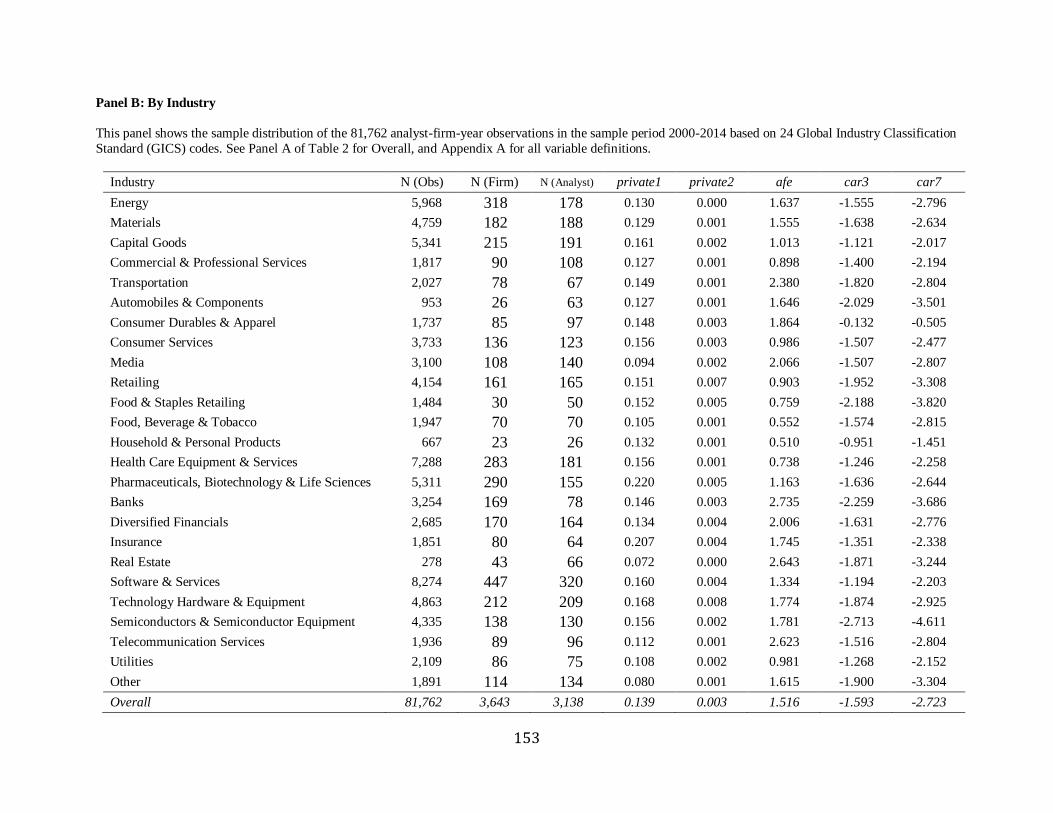
153

Panel B: By Industry

This panel shows the sample distribution of the 81,762 analyst-firm-year observations in the sample period 2000-2014 based on 24 Global Industry Classification

Standard (GICS) codes. See Panel A of Table 2 for Overall, and Appendix A for all variable definitions.

Industry N (Obs) N (Firm) N (Analyst) private1 private2 afe car3 car7

Energy 5,968 318 178 0.130 0.000 1.637 -1.555 -2.796

Materials 4,759 182 188 0.129 0.001 1.555 -1.638 -2.634

Capital Goods 5,341 215 191 0.161 0.002 1.013 -1.121 -2.017

Commercial & Professional Services 1,817 90 108 0.127 0.001 0.898 -1.400 -2.194

Transportation 2,027 78 67 0.149 0.001 2.380 -1.820 -2.804

Automobiles & Components 953 26 63 0.127 0.001 1.646 -2.029 -3.501

Consumer Durables & Apparel 1,737 85 97 0.148 0.003 1.864 -0.132 -0.505

Consumer Services 3,733 136 123 0.156 0.003 0.986 -1.507 -2.477

Media 3,100 108 140 0.094 0.002 2.066 -1.507 -2.807

Retailing 4,154 161 165 0.151 0.007 0.903 -1.952 -3.308

Food & Staples Retailing 1,484 30 50 0.152 0.005 0.759 -2.188 -3.820

Food, Beverage & Tobacco 1,947 70 70 0.105 0.001 0.552 -1.574 -2.815

Household & Personal Products 667 23 26 0.132 0.001 0.510 -0.951 -1.451

Health Care Equipment & Services 7,288 283 181 0.156 0.001 0.738 -1.246 -2.258

Pharmaceuticals, Biotechnology & Life Sciences 5,311 290 155 0.220 0.005 1.163 -1.636 -2.644

Banks 3,254 169 78 0.146 0.003 2.735 -2.259 -3.686

Diversified Financials 2,685 170 164 0.134 0.004 2.006 -1.631 -2.776

Insurance 1,851 80 64 0.207 0.004 1.745 -1.351 -2.338

Real Estate 278 43 66 0.072 0.000 2.643 -1.871 -3.244

Software & Services 8,274 447 320 0.160 0.004 1.334 -1.194 -2.203

Technology Hardware & Equipment 4,863 212 209 0.168 0.008 1.774 -1.874 -2.925

Semiconductors & Semiconductor Equipment 4,335 138 130 0.156 0.002 1.781 -2.713 -4.611

Telecommunication Services 1,936 89 96 0.112 0.001 2.623 -1.516 -2.804

Utilities 2,109 86 75 0.108 0.002 0.981 -1.268 -2.152

Other 1,891 114 134 0.080 0.001 1.615 -1.900 -3.304

Overall 81,762 3,643 3,138 0.139 0.003 1.516 -1.593 -2.723

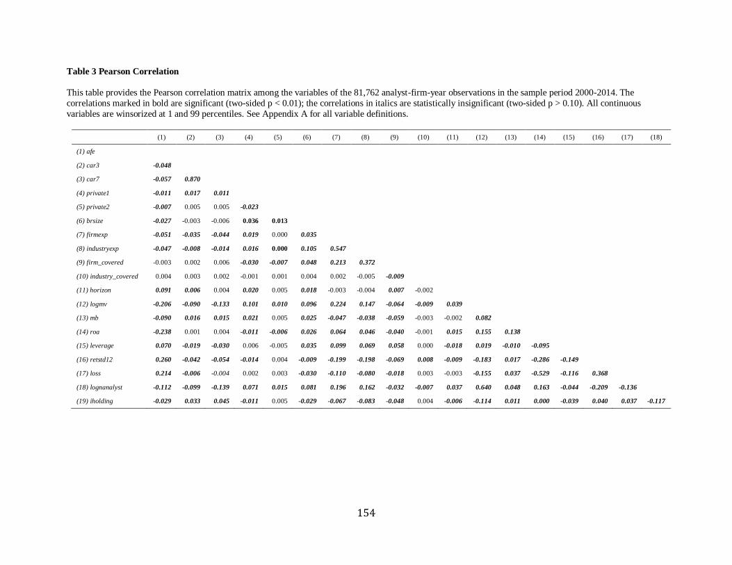
154

Table 3 Pearson Correlation

This table provides the Pearson correlation matrix among the variables of the 81,762 analyst-firm-year observations in the sample period 2000-2014. The

correlations marked in bold are significant (two-sided p < 0.01); the correlations in italics are statistically insignificant (two-sided p > 0.10). All continuous

variables are winsorized at 1 and 99 percentiles. See Appendix A for all variable definitions.

(1) (2) (3) (4) (5) (6) (7) (8) (9) (10) (11) (12) (13) (14) (15) (16) (17) (18)

(1) afe

(2) car3 -0.048

(3) car7 -0.057 0.870

(4) private1 -0.011 0.017 0.011

(5) private2 -0.007 0.005 0.005 -0.023

(6) brsize -0.027 -0.003 -0.006 0.036 0.013

(7) firmexp -0.051 -0.035 -0.044 0.019 0.000 0.035

(8) industryexp -0.047 -0.008 -0.014 0.016 0.000 0.105 0.547

(9) firm_covered -0.003 0.002 0.006 -0.030 -0.007 0.048 0.213 0.372

(10) industry_covered 0.004 0.003 0.002 -0.001 0.001 0.004 0.002 -0.005 -0.009

(11) horizon 0.091 0.006 0.004 0.020 0.005 0.018 -0.003 -0.004 0.007 -0.002

(12) logmv -0.206 -0.090 -0.133 0.101 0.010 0.096 0.224 0.147 -0.064 -0.009 0.039

(13) mb -0.090 0.016 0.015 0.021 0.005 0.025 -0.047 -0.038 -0.059 -0.003 -0.002 0.082

(14) roa -0.238 0.001 0.004 -0.011 -0.006 0.026 0.064 0.046 -0.040 -0.001 0.015 0.155 0.138

(15) leverage 0.070 -0.019 -0.030 0.006 -0.005 0.035 0.099 0.069 0.058 0.000 -0.018 0.019 -0.010 -0.095

(16) retstd12 0.260 -0.042 -0.054 -0.014 0.004 -0.009 -0.199 -0.198 -0.069 0.008 -0.009 -0.183 0.017 -0.286 -0.149

(17) loss 0.214 -0.006 -0.004 0.002 0.003 -0.030 -0.110 -0.080 -0.018 0.003 -0.003 -0.155 0.037 -0.529 -0.116 0.368

(18) lognanalyst -0.112 -0.099 -0.139 0.071 0.015 0.081 0.196 0.162 -0.032 -0.007 0.037 0.640 0.048 0.163 -0.044 -0.209 -0.136

(19) iholding -0.029 0.033 0.045 -0.011 0.005 -0.029 -0.067 -0.083 -0.048 0.004 -0.006 -0.114 0.011 0.000 -0.039 0.040 0.037 -0.117

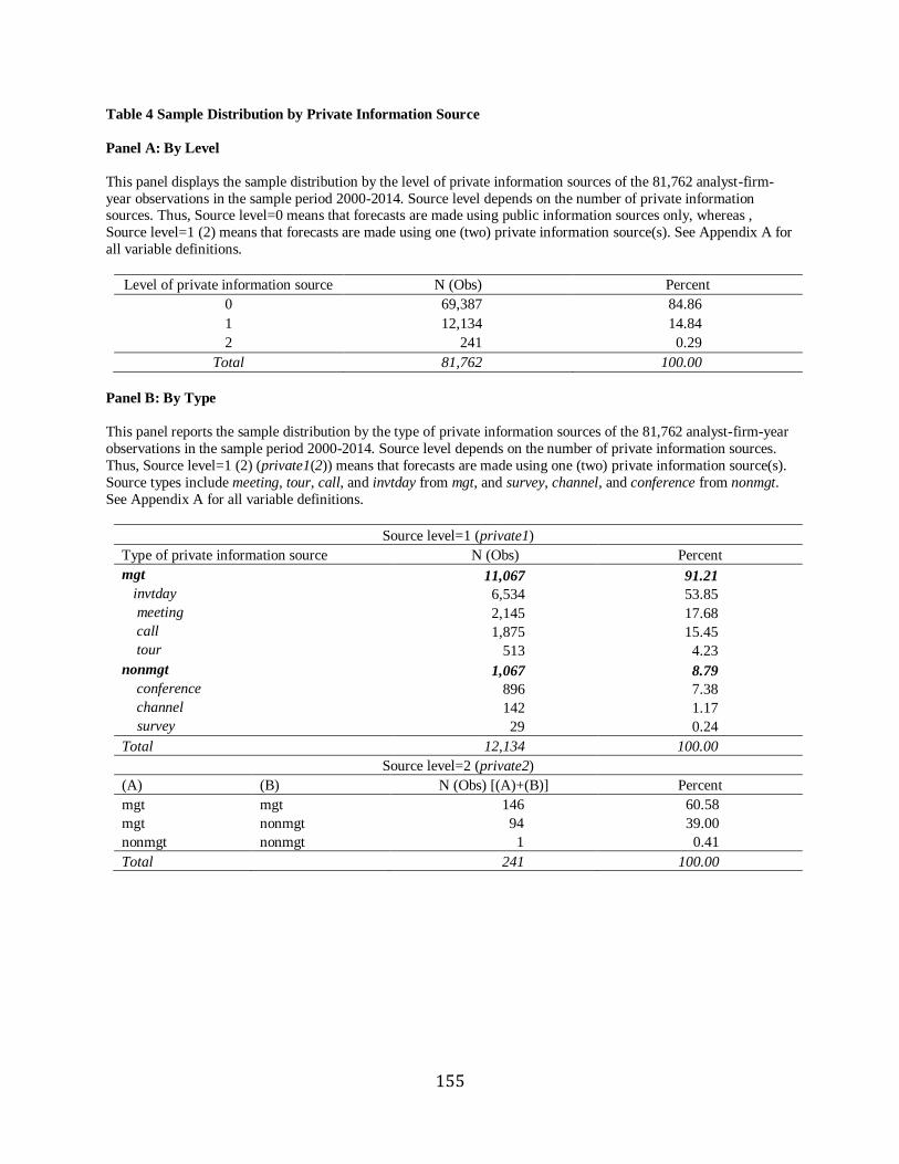
155

Table 4 Sample Distribution by Private Information Source

Panel A: By Level

This panel displays the sample distribution by the level of private information sources of the 81,762 analyst-firm-

year observations in the sample period 2000-2014. Source level depends on the number of private information sources. Thus, Source level=0 means that forecasts are made using public information sources only, whereas ,

Source level=1 (2) means that forecasts are made using one (two) private information source(s). See Appendix A for

all variable definitions.

Level of private information source N (Obs) Percent

0 69,387 84.86

1 12,134 14.84

2 241 0.29

Total 81,762 100.00

Panel B: By Type

This panel reports the sample distribution by the type of private information sources of the 81,762 analyst-firm-year

observations in the sample period 2000-2014. Source level depends on the number of private information sources.

Thus, Source level=1 (2) (private1(2)) means that forecasts are made using one (two) private information source(s).

Source types include meeting, tour, call, and invtday from mgt, and survey, channel, and conference from nonmgt.

See Appendix A for all variable definitions.

Source level=1 (private1)

Type of private information source N (Obs) Percent

mgt 11,067 91.21

invtday 6,534 53.85

meeting 2,145 17.68

call 1,875 15.45

tour 513 4.23

nonmgt 1,067 8.79

conference 896 7.38

channel 142 1.17

survey 29 0.24

Total 12,134 100.00

Source level=2 (private2)

(A) (B) N (Obs) [(A)+(B)] Percent

mgt mgt 146 60.58

mgt nonmgt 94 39.00

nonmgt nonmgt 1 0.41

Total 241 100.00

156

Panel C: Detailed Distribution by Source Level=2

This panel provides the detailed sample distribution by two sources of private information of the 81,762 analyst-firm-year observations in the sample period

2000-2014. Source level depends on the number of private information sources. Thus, Source level=2 (private2) means that forecasts are made using two private

information sources. Source types include meeting, tour, call, and invtday from mgt, and survey, channel, and conference from nonmgt. meetinginvtday

represents forecasts based on two management-related private information sources from both personal meetings with management and investor/analyst days. See Appendix A for all variable definitions.

Source level=2 (private2)

Variable Source N (obs) N (firm) N (analyst) Mean Std Dev Q1 Median Q3

meetinginvtday mgt+mgt 96 80 54 0.001 0.034 0.000 0.000 0.000

invtdayconference mgt+nonmgt 72 65 41 0.001 0.030 0.000 0.000 0.000

meetingtour mgt+mgt 17 14 16 0.000 0.014 0.000 0.000 0.000

tourinvtday mgt+mgt 12 12 11 0.000 0.012 0.000 0.000 0.000

callinvtday mgt+mgt 11 10 9 0.000 0.012 0.000 0.000 0.000

callconference mgt+nonmgt 11 8 7 0.000 0.012 0.000 0.000 0.000

meetingcall mgt+mgt 10 10 10 0.000 0.011 0.000 0.000 0.000

meetingconference mgt+nonmgt 4 4 4 0.000 0.007 0.000 0.000 0.000

invtdaychannel mgt+nonmgt 3 2 1 0.000 0.006 0.000 0.000 0.000

meetingchannel mgt+nonmgt 3 3 2 0.000 0.006 0.000 0.000 0.000

callchannel mgt+nonmgt 1 1 1 0.000 0.003 0.000 0.000 0.000

channelconference nonmgt+nonmgt 1 1 1 0.000 0.003 0.000 0.000 0.000

Overall 241 210 157 0.000 0.013 0.000 0.000 0.000

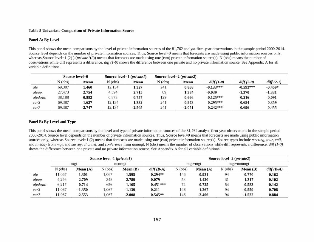
157

Table 5 Univariate Comparison of Private Information Source

Panel A: By Level

This panel shows the mean comparisons by the level of private information sources of the 81,762 analyst-firm-year observations in the sample period 2000-2014.

Source level depends on the number of private information sources. Thus, Source level=0 means that forecasts are made using public information sources only, whereas Source level=1 (2) ) (private1(2)) means that forecasts are made using one (two) private information source(s). N (obs) means the number of

observations while diff represents a difference. diff (1-0) shows the difference between one private and no private information source. See Appendix A for all

variable definitions.

Source level=0 Source level=1 (private1) Source level=2 (private2)

N (obs) Mean N (obs) Mean N (obs) Mean diff (1-0) diff (2-0) diff (2-1)

afe 69,387 1.460 12,134 1.327 241 0.868 -0.133*** -0.592*** -0.459*

afeup 27,473 2.754 4,594 2.715 89 1.384 -0.039 -1.370 -1.331

afedown 38,188 0.882 6,873 0.757 129 0.666 -0.125*** -0.216 -0.091

car3 69,387 -1.627 12,134 -1.332 241 -0.973 0.295*** 0.654 0.359

car7 69,387 -2.747 12,134 -2.505 241 -2.051 0.242*** 0.696 0.455

Panel B: By Level and Type

This panel shows the mean comparisons by the level and type of private information sources of the 81,762 analyst-firm-year observations in the sample period

2000-2014. Source level depends on the number of private information sources. Thus, Source level=0 means that forecasts are made using public information

sources only, whereas Source level=1 (2) means that forecasts are made using one (two) private information source(s). Source types include meeting, tour, call,

and invtday from mgt, and survey, channel, and conference from nonmgt. N (obs) means the number of observations while diff represents a difference. diff (1-0)

shows the difference between one private and no private information source. See Appendix A for all variable definitions.

Source level=1 (private1) Source level=2 (private2)

mgt nonmgt mgt+mgt mgt+nonmgt

N (obs) Mean (A) N (obs) Mean (B) diff (B-A) N (obs) Mean (A) N (obs) Mean (B) diff (B-A)

afe 11,067 1.301 1,067 1.595 0.294** 146 0.931 94 0.770 -0.162

afeup 4,246 2.709 348 2.789 0.079 58 1.420 31 1.317 -0.102

afedown 6,217 0.714 656 1.165 0.451*** 74 0.725 54 0.583 -0.142

car3 11,067 -1.350 1,067 -1.139 0.211 146 -1.267 94 -0.559 0.708

car7 11,067 -2.553 1,067 -2.008 0.545** 146 -2.406 94 -1.522 0.884

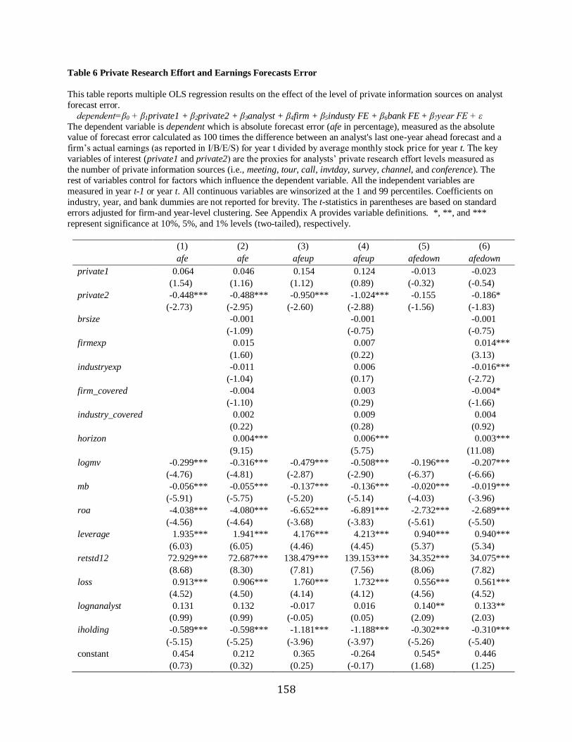
158

Table 6 Private Research Effort and Earnings Forecasts Error

This table reports multiple OLS regression results on the effect of the level of private information sources on analyst

forecast error.

dependent=β0 + β1private1 + β2private2 + β3analyst + β4firm + β5industy FE + β6bank FE + β7year FE + ε

The dependent variable is dependent which is absolute forecast error (afe in percentage), measured as the absolute value of forecast error calculated as 100 times the difference between an analyst's last one-year ahead forecast and a

firm’s actual earnings (as reported in I/B/E/S) for year t divided by average monthly stock price for year t. The key

variables of interest (private1 and private2) are the proxies for analysts’ private research effort levels measured as

the number of private information sources (i.e., meeting, tour, call, invtday, survey, channel, and conference). The

rest of variables control for factors which influence the dependent variable. All the independent variables are

measured in year t-1 or year t. All continuous variables are winsorized at the 1 and 99 percentiles. Coefficients on

industry, year, and bank dummies are not reported for brevity. The t-statistics in parentheses are based on standard

errors adjusted for firm-and year-level clustering. See Appendix A provides variable definitions. *, **, and ***

represent significance at 10%, 5%, and 1% levels (two-tailed), respectively.

(1) (2) (3) (4) (5) (6)

afe afe afeup afeup afedown afedown

private1 0.064 0.046 0.154 0.124 -0.013 -0.023

(1.54) (1.16) (1.12) (0.89) (-0.32) (-0.54)

private2 -0.448*** -0.488*** -0.950*** -1.024*** -0.155 -0.186*

(-2.73) (-2.95) (-2.60) (-2.88) (-1.56) (-1.83)

brsize -0.001 -0.001 -0.001

(-1.09) (-0.75) (-0.75)

firmexp 0.015 0.007 0.014***

(1.60) (0.22) (3.13)

industryexp -0.011 0.006 -0.016***

(-1.04) (0.17) (-2.72)

firm_covered -0.004 0.003 -0.004*

(-1.10) (0.29) (-1.66)

industry_covered 0.002 0.009 0.004

(0.22) (0.28) (0.92)

horizon 0.004*** 0.006*** 0.003***

(9.15) (5.75) (11.08)

logmv -0.299*** -0.316*** -0.479*** -0.508*** -0.196*** -0.207***

(-4.76) (-4.81) (-2.87) (-2.90) (-6.37) (-6.66)

mb -0.056*** -0.055*** -0.137*** -0.136*** -0.020*** -0.019***

(-5.91) (-5.75) (-5.20) (-5.14) (-4.03) (-3.96)

roa -4.038*** -4.080*** -6.652*** -6.891*** -2.732*** -2.689***

(-4.56) (-4.64) (-3.68) (-3.83) (-5.61) (-5.50)

leverage 1.935*** 1.941*** 4.176*** 4.213*** 0.940*** 0.940***

(6.03) (6.05) (4.46) (4.45) (5.37) (5.34)

retstd12 72.929*** 72.687*** 138.479*** 139.153*** 34.352*** 34.075***

(8.68) (8.30) (7.81) (7.56) (8.06) (7.82)

loss 0.913*** 0.906*** 1.760*** 1.732*** 0.556*** 0.561***

(4.52) (4.50) (4.14) (4.12) (4.56) (4.52)

lognanalyst 0.131 0.132 -0.017 0.016 0.140** 0.133**

(0.99) (0.99) (-0.05) (0.05) (2.09) (2.03)

iholding -0.589*** -0.598*** -1.181*** -1.188*** -0.302*** -0.310***

(-5.15) (-5.25) (-3.96) (-3.97) (-5.26) (-5.40)

constant 0.454 0.212 0.365 -0.264 0.545* 0.446

(0.73) (0.32) (0.25) (-0.17) (1.68) (1.25)

159

industry f.e. yes yes yes yes yes yes

year f.e. yes yes yes yes yes yes

bank f.e. yes yes yes yes yes yes

clustering firm-year firm-year firm-year firm-year firm-year firm-year

observations 81,762 81,762 32,156 32,156 45,190 45,190

adjusted R2 0.147 0.156 0.134 0.138 0.187 0.203

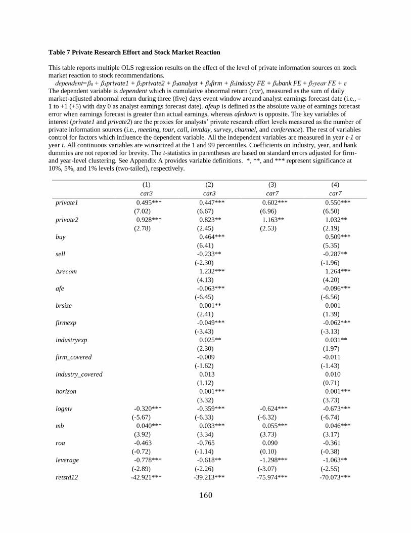
160

Table 7 Private Research Effort and Stock Market Reaction

This table reports multiple OLS regression results on the effect of the level of private information sources on stock

market reaction to stock recommendations.

dependent=β0 + β1private1 + β2private2 + β3analyst + β4firm + β5industy FE + β6bank FE + β7year FE + ε

The dependent variable is dependent which is cumulative abnormal return (car), measured as the sum of daily market-adjusted abnormal return during three (five) days event window around analyst earnings forecast date (i.e., -

1 to +1 (+5) with day 0 as analyst earnings forecast date). afeup is defined as the absolute value of earnings forecast

error when earnings forecast is greater than actual earnings, whereas afedown is opposite. The key variables of

interest (private1 and private2) are the proxies for analysts’ private research effort levels measured as the number of

private information sources (i.e., meeting, tour, call, invtday, survey, channel, and conference). The rest of variables

control for factors which influence the dependent variable. All the independent variables are measured in year t-1 or

year t. All continuous variables are winsorized at the 1 and 99 percentiles. Coefficients on industry, year, and bank

dummies are not reported for brevity. The t-statistics in parentheses are based on standard errors adjusted for firm-

and year-level clustering. See Appendix A provides variable definitions. *, **, and *** represent significance at

10%, 5%, and 1% levels (two-tailed), respectively.

(1) (2) (3) (4)

car3 car3 car7 car7

private1 0.495*** 0.447*** 0.602*** 0.550***

(7.02) (6.67) (6.96) (6.50)

private2 0.928*** 0.823** 1.163** 1.032**

(2.78) (2.45) (2.53) (2.19)

buy 0.464*** 0.509***

(6.41) (5.35)

sell -0.233** -0.287**

(-2.30) (-1.96)

∆recom 1.232*** 1.264***

(4.13) (4.20)

afe -0.063*** -0.096***

(-6.45) (-6.56)

brsize 0.001** 0.001

(2.41) (1.39)

firmexp -0.049*** -0.062***

(-3.43) (-3.13)

industryexp 0.025** 0.031**

(2.30) (1.97)

firm_covered -0.009 -0.011

(-1.62) (-1.43)

industry_covered 0.013 0.010

(1.12) (0.71)

horizon 0.001*** 0.001***

(3.32) (3.73)

logmv -0.320*** -0.359*** -0.624*** -0.673***

(-5.67) (-6.33) (-6.32) (-6.74)

mb 0.040*** 0.033*** 0.055*** 0.046***

(3.92) (3.34) (3.73) (3.17)

roa -0.463 -0.765 0.090 -0.361

(-0.72) (-1.14) (0.10) (-0.38)

leverage -0.778*** -0.618** -1.298*** -1.063**

(-2.89) (-2.26) (-3.07) (-2.55)

retstd12 -42.921*** -39.213*** -75.974*** -70.073***

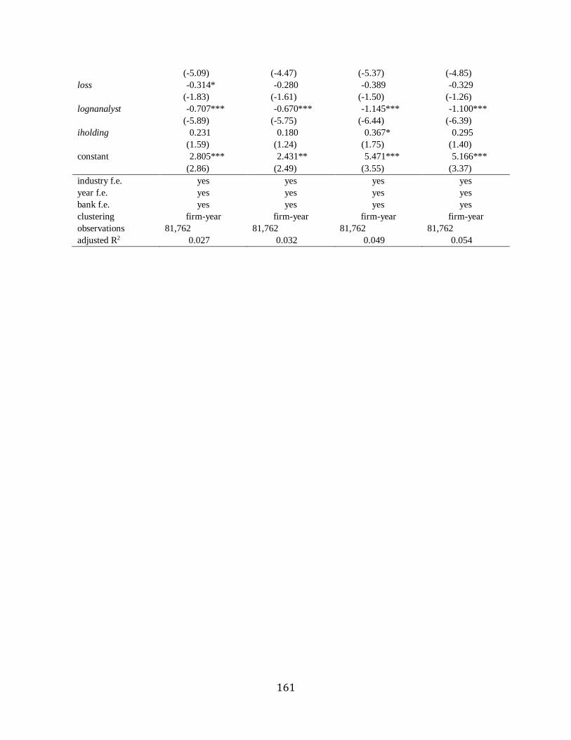
161

(-5.09) (-4.47) (-5.37) (-4.85)

loss -0.314* -0.280 -0.389 -0.329

(-1.83) (-1.61) (-1.50) (-1.26)

lognanalyst -0.707*** -0.670*** -1.145*** -1.100***

(-5.89) (-5.75) (-6.44) (-6.39)

iholding 0.231 0.180 0.367* 0.295

(1.59) (1.24) (1.75) (1.40)

constant 2.805*** 2.431** 5.471*** 5.166***

(2.86) (2.49) (3.55) (3.37)

industry f.e. yes yes yes yes

year f.e. yes yes yes yes

bank f.e. yes yes yes yes

clustering firm-year firm-year firm-year firm-year

observations 81,762 81,762 81,762 81,762

adjusted R2 0.027 0.032 0.049 0.054

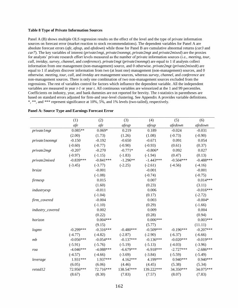
162

Table 8 Type of Private Information Sources

Panel A (B) shows multiple OLS regression results on the effect of the level and the type of private information

sources on forecast error (market reaction to stock recommendations). The dependent variables for Panel A are

absolute forecast errors (afe, afeup, and afedown) while those for Panel B are cumulative abnormal returns (car3 and

car7). The key variables of interest (private1mgt, private1nonmgt, private2mgt and private2mixed) are the proxies for analysts’ private research effort levels measured as the number of private information sources (i.e., meeting, tour,

call, invtday, survey, channel, and conference). private1mgt (private1nonmgt) are equal to 1 if analysts collect

information from one management (non-management) source, and 0 otherwise. private2mgt (private2mixedt) are

equal to 1 if analysts discover information from two (at least one) management (non-management) sources, and 0

otherwise. meeting, tour, call, and invtday are management sources, whereas survey, channel, and conference are

non-management sources. There is only one combination of two non-management sources excluded from the

regressions. The rest of variables control for factors which influence the dependent variable. All the independent

variables are measured in year t-1 or year t. All continuous variables are winsorized at the 1 and 99 percentiles.

Coefficients on industry, year, and bank dummies are not reported for brevity. The t-statistics in parentheses are

based on standard errors adjusted for firm-and year-level clustering. See Appendix A provides variable definitions.

*, **, and *** represent significance at 10%, 5%, and 1% levels (two-tailed), respectively.

Panel A: Source Type and Earnings Forecast Error

(1) (2) (3) (4) (5) (6)

afe afe afeup afeup afedown afedown

private1mgt 0.085** 0.069* 0.219 0.189 -0.024 -0.031

(2.00) (1.73) (1.26) (1.08) (-0.73) (-0.90)

private1nonmgt -0.150 -0.192 -0.650 -0.671 0.091 0.054

(-0.60) (-0.77) (-0.90) (-0.93) (0.61) (0.37)

private2mgt -0.207 -0.270 -0.771* -0.806* 0.092 0.027

(-0.97) (-1.15) (-1.83) (-1.94) (0.47) (0.13)

private2mixed -0.839*** -0.841*** -1.296** -1.443*** -0.504*** -0.488***

(-3.45) (-3.77) (-2.25) (-2.61) (-4.56) (-4.16)

brsize -0.001 -0.001 -0.001

(-1.08) (-0.74) (-0.75)

firmexp 0.015 0.007 0.014***

(1.60) (0.23) (3.11)

industryexp -0.011 0.006 -0.016***

(-1.04) (0.17) (-2.72)

firm_covered -0.004 0.003 -0.004*

(-1.10) (0.29) (-1.66)

industry_covered 0.002 0.009 0.004

(0.22) (0.28) (0.94)

horizon 0.004*** 0.006*** 0.003***

(9.15) (5.77) (11.11)

logmv -0.299*** -0.316*** -0.480*** -0.509*** -0.196*** -0.207***

(-4.77) (-4.82) (-2.87) (-2.90) (-6.37) (-6.66)

mb -0.056*** -0.054*** -0.137*** -0.136*** -0.020*** -0.019***

(-5.91) (-5.76) (-5.19) (-5.13) (-4.03) (-3.96)

roa -4.046*** -4.088*** -6.679*** -6.918*** -2.727*** -2.686***

(-4.57) (-4.66) (-3.69) (-3.84) (-5.59) (-5.49)

leverage 1.931*** 1.937*** 4.162*** 4.199*** 0.940*** 0.940***

(6.05) (6.06) (4.46) (4.45) (5.38) (5.34)

retstd12 72.956*** 72.716*** 138.547*** 139.222*** 34.350*** 34.075***

(8.67) (8.30) (7.83) (7.57) (8.07) (7.83)

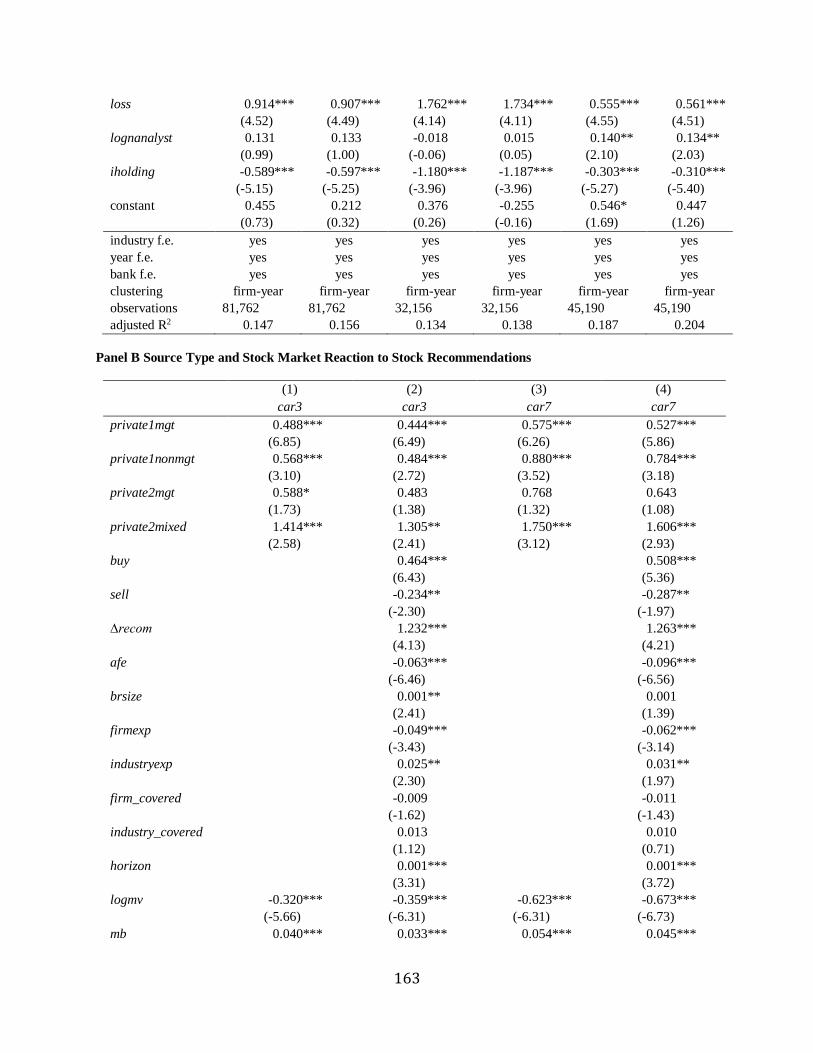
163

loss 0.914*** 0.907*** 1.762*** 1.734*** 0.555*** 0.561***

(4.52) (4.49) (4.14) (4.11) (4.55) (4.51)

lognanalyst 0.131 0.133 -0.018 0.015 0.140** 0.134**

(0.99) (1.00) (-0.06) (0.05) (2.10) (2.03)

iholding -0.589*** -0.597*** -1.180*** -1.187*** -0.303*** -0.310***

(-5.15) (-5.25) (-3.96) (-3.96) (-5.27) (-5.40)

constant 0.455 0.212 0.376 -0.255 0.546* 0.447

(0.73) (0.32) (0.26) (-0.16) (1.69) (1.26)

industry f.e. yes yes yes yes yes yes

year f.e. yes yes yes yes yes yes

bank f.e. yes yes yes yes yes yes

clustering firm-year firm-year firm-year firm-year firm-year firm-year

observations 81,762 81,762 32,156 32,156 45,190 45,190

adjusted R2 0.147 0.156 0.134 0.138 0.187 0.204

Panel B Source Type and Stock Market Reaction to Stock Recommendations

(1) (2) (3) (4)

car3 car3 car7 car7

private1mgt 0.488*** 0.444*** 0.575*** 0.527***

(6.85) (6.49) (6.26) (5.86)

private1nonmgt 0.568*** 0.484*** 0.880*** 0.784***

(3.10) (2.72) (3.52) (3.18)

private2mgt 0.588* 0.483 0.768 0.643

(1.73) (1.38) (1.32) (1.08)

private2mixed 1.414*** 1.305** 1.750*** 1.606***

(2.58) (2.41) (3.12) (2.93)

buy 0.464*** 0.508***

(6.43) (5.36)

sell -0.234** -0.287**

(-2.30) (-1.97)

∆recom 1.232*** 1.263***

(4.13) (4.21)

afe -0.063*** -0.096***

(-6.46) (-6.56)

brsize 0.001** 0.001

(2.41) (1.39)

firmexp -0.049*** -0.062***

(-3.43) (-3.14)

industryexp 0.025** 0.031**

(2.30) (1.97)

firm_covered -0.009 -0.011

(-1.62) (-1.43)

industry_covered 0.013 0.010

(1.12) (0.71)

horizon 0.001*** 0.001***

(3.31) (3.72)

logmv -0.320*** -0.359*** -0.623*** -0.673***

(-5.66) (-6.31) (-6.31) (-6.73)

mb 0.040*** 0.033*** 0.054*** 0.045***

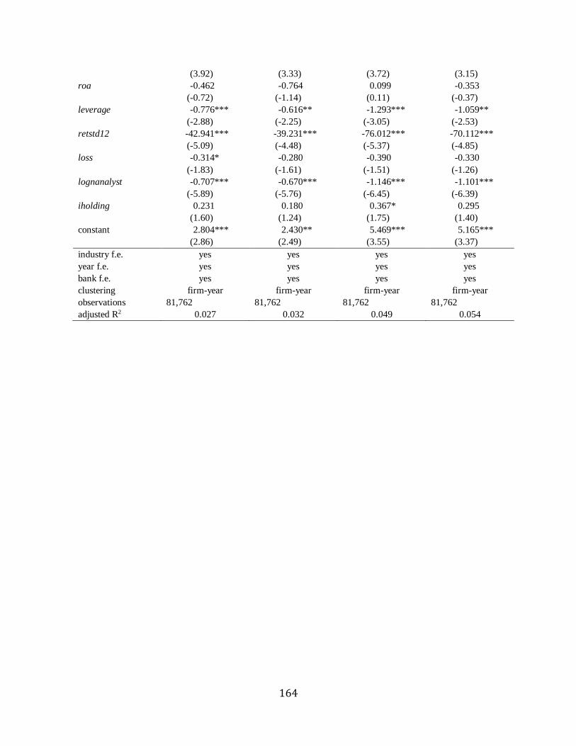
164

(3.92) (3.33) (3.72) (3.15)

roa -0.462 -0.764 0.099 -0.353

(-0.72) (-1.14) (0.11) (-0.37)

leverage -0.776*** -0.616** -1.293*** -1.059**

(-2.88) (-2.25) (-3.05) (-2.53)

retstd12 -42.941*** -39.231*** -76.012*** -70.112***

(-5.09) (-4.48) (-5.37) (-4.85)

loss -0.314* -0.280 -0.390 -0.330

(-1.83) (-1.61) (-1.51) (-1.26)

lognanalyst -0.707*** -0.670*** -1.146*** -1.101***

(-5.89) (-5.76) (-6.45) (-6.39)

iholding 0.231 0.180 0.367* 0.295

(1.60) (1.24) (1.75) (1.40)

constant 2.804*** 2.430** 5.469*** 5.165***

(2.86) (2.49) (3.55) (3.37)

industry f.e. yes yes yes yes

year f.e. yes yes yes yes

bank f.e. yes yes yes yes

clustering firm-year firm-year firm-year firm-year

observations 81,762 81,762 81,762 81,762

adjusted R2 0.027 0.032 0.049 0.054

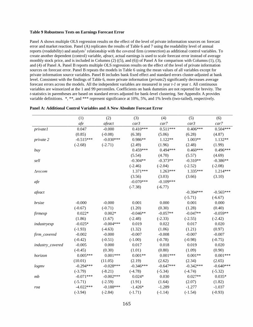
165

Table 9 Robustness Tests on Earnings Forecast Error

Panel A shows multiple OLS regression results on the effect of the level of private information sources on forecast

error and market reaction. Panel (A) replicates the results of Table 6 and 7 using the readability level of annual

reports (readability) and analysts’ relationship with the covered firm (connection) as additional control variables. To

create another dependent (control) variable, afeact, actual earnings is used to scale forecast error instead of average monthly stock price, and is included in Columns (2) ((5), and (6)) of Panel A for comparison with Columns (1), (3),

and (4) of Panel A. Panel B reports multiple OLS regression results on the effect of the level of private information

sources on forecast error. Panel B repeats the models in Table 6 using the mean values of all variables except for

private information source variables. Panel B includes bank fixed effect and standard errors cluster-adjusted at bank

level. Consistent with the findings of Table 6, more private information (private2) significantly decreases average

forecast errors across the models. All the independent variables are measured in year t-1 or year t. All continuous

variables are winsorized at the 1 and 99 percentiles. Coefficients on bank dummies are not reported for brevity. The

t-statistics in parentheses are based on standard errors adjusted for bank-level clustering. See Appendix A provides

variable definitions. *, **, and *** represent significance at 10%, 5%, and 1% levels (two-tailed), respectively.

Panel A: Additional Control Variables and A New Absolute Forecast Error

(1) (2) (3) (4) (5) (6)

afe afeact car3 car7 car3 car7

private1 0.047 -0.000 0.410*** 0.511*** 0.406*** 0.504***

(0.85) (-0.08) (6.38) (5.06) (6.28) (4.87)

private 2 -0.515*** -0.030*** 0.986** 1.122** 1.003** 1.132**

(-2.68) (-2.71) (2.49) (1.96) (2.48) (1.99)

buy 0.459*** 0.494*** 0.460*** 0.496***

(5.54) (4.70) (5.57) (4.69)

sell -0.304** -0.373** -0.310** -0.386**

(-2.46) (-2.04) (-2.52) (-2.08)

∆recom 1.371*** 1.263*** 1.335*** 1.214***

(3.56) (3.03) (3.66) (3.10)

afe -0.070*** -0.109***

(-7.38) (-6.77)

afeact -0.394*** -0.565***

(-5.71) (-6.67)

brsize -0.000 -0.000 0.001 0.000 0.001 0.000

(-0.67) (-0.71) (1.20) (0.30) (1.28) (0.40)

firmexp 0.022* 0.002* -0.046** -0.057** -0.047** -0.059**

(1.86) (1.67) (-2.48) (-2.33) (-2.55) (-2.42)

industryexp -0.025* -0.004*** 0.019 0.022 0.017 0.020

(-1.93) (-4.63) (1.32) (1.06) (1.21) (0.97)

firm_covered -0.002 -0.000 -0.007 -0.008 -0.007 -0.007

(-0.42) (-0.51) (-1.00) (-0.78) (-0.98) (-0.75)

industry_covered -0.005 0.000 0.017 0.018 0.019 0.020

(-0.45) (0.30) (1.01) (0.80) (1.09) (0.90)

horizon 0.005*** 0.001*** 0.001** 0.001*** 0.001** 0.001***

(10.01) (11.05) (2.19) (2.62) (2.34) (2.65)

logmv -0.294*** -0.028*** -0.346*** -0.647*** -0.342*** -0.640***

(-3.79) (-8.21) (-4.78) (-5.34) (-4.74) (-5.32)

mb -0.071*** -0.002*** 0.024* 0.030 0.027** 0.035*

(-5.71) (-2.59) (1.91) (1.64) (2.07) (1.82)

roa -4.022*** -0.188*** -1.426* -1.289 -1.277 -1.037

(-3.94) (-2.84) (-1.71) (-1.14) (-1.54) (-0.93)

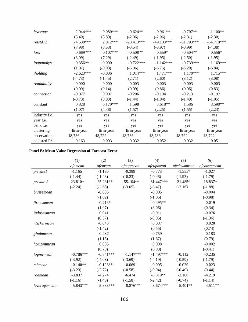
166

leverage 2.044*** 0.080*** -0.624** -0.961** -0.707** -1.100**

(5.40) (3.89) (-2.06) (-2.06) (-2.31) (-2.30)

retstd12 74.538*** 2.812*** -28.410*** -49.133*** -31.790*** -54.718***

(7.98) (8.53) (-3.54) (-3.97) (-3.99) (-4.38)

loss 0.669*** 0.107*** -0.508** -0.559* -0.504** -0.556*

(3.09) (7.29) (-2.49) (-1.95) (-2.50) (-1.95)

lognanalyst 0.356** -0.000 -0.722*** -1.142*** -0.739*** -1.169***

(1.97) (-0.03) (-5.06) (-5.75) (-5.20) (-5.84)

iholding -2.623*** -0.036 1.014*** 1.471*** 1.170*** 1.715***

(-4.73) (-1.45) (2.71) (2.60) (3.12) (3.08)

readability 0.000 0.000 0.003 0.003 0.003 0.003

(0.09) (0.14) (0.99) (0.86) (0.96) (0.83)

connection -0.077 0.007 -0.206 -0.194 -0.213 -0.197

(-0.73) (0.83) (-1.44) (-1.04) (-1.49) (-1.05)

constant 0.828 0.170*** 1.598 3.618** 1.586 3.590**

(1.07) (4.38) (1.57) (2.25) (1.55) (2.23)

industry f.e. yes yes yes yes yes yes

year f.e. yes yes yes yes yes yes

bank f.e. yes yes yes yes yes yes

clustering firm-year firm-year firm-year firm-year firm-year firm-year

observations 48,786 48,722 48,786 48,786 48,722 48,722

adjusted R2 0.163 0.093 0.032 0.052 0.032 0.051

Panel B: Mean Value Regression of Forecast Error

(1) (2) (3) (4) (5) (6)

afemean afemean afeupmean afeupmean afedownmean afedownmean

private1 -1.165 -1.180 -0.389 -0.773 -1.555* -1.027

(-1.44) (-1.43) (-0.23) (-0.48) (-1.93) (-1.79)

private 2 -23.810* -25.231** -55.104** -61.447*** -21.485* -18.837*

(-2.24) (-2.68) (-3.05) (-3.47) (-2.16) (-1.88)

brsizemean -0.006 -0.005 -0.004

(-1.62) (-1.05) (-0.98)

firmexmean 0.218* 0.495** 0.019

(1.97) (3.06) (0.34)

indusexmean 0.041 -0.011 -0.076

(0.37) (-0.05) (-1.36)

ntickermean -0.040 0.037 0.020

(-1.42) (0.55) (0.74)

gindnmean 0.487 0.759 0.183

(1.15) (1.67) (0.79)

horizonmean 0.005 0.008 -0.002

(0.78) (0.83) (-0.41)

logmvmean -0.786*** -0.841*** -1.147*** -1.497*** -0.112 -0.235

(-3.92) (-4.03) (-3.69) (-4.19) (-0.59) (-1.79)

mbmean -0.140** -0.128** -0.069 -0.005 -0.029 0.023

(-3.23) (-2.72) (-0.58) (-0.04) (-0.40) (0.44)

roamean -3.837 -4.274 -6.474 -8.319** -3.186 -4.219

(-1.16) (-1.43) (-1.58) (-2.42) (-0.74) (-1.14)

leveragemean 5.843*** 5.888*** 8.876*** 8.674*** 5.401** 4.511**

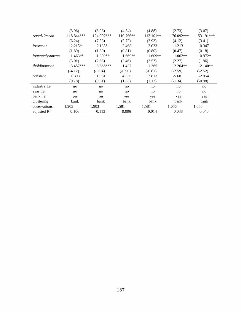
167

(3.96) (3.96) (4.54) (4.88) (2.73) (3.07)

retstd12mean 118.844*** 124.097*** 110.766** 112.101** 176.092*** 153.191***

(6.24) (7.58) (2.72) (2.93) (4.12) (3.41)

lossmean 2.215* 2.135* 2.468 2.033 1.213 0.347

(1.89) (1.89) (0.81) (0.80) (0.47) (0.18)

lognanalystmean 1.463** 1.399** 1.669** 1.609** 1.062** 0.972*

(3.01) (2.83) (2.46) (2.53) (2.27) (1.96)

iholdingmean -3.457*** -3.665*** -1.427 -1.365 -2.264** -2.140**

(-4.12) (-3.94) (-0.90) (-0.81) (-2.59) (-2.52)

constant 1.393 1.061 4.336 3.813 -5.681 -2.954

(0.78) (0.51) (1.63) (1.12) (-1.34) (-0.98)

industry f.e. no no no no no no

year f.e. no no no no no no

bank f.e. yes yes yes yes yes yes

clustering bank bank bank bank bank bank

observations 1,903 1,903 1,581 1,581 1,656 1,656

adjusted R2 0.106 0.113 0.006 0.014 0.038 0.040

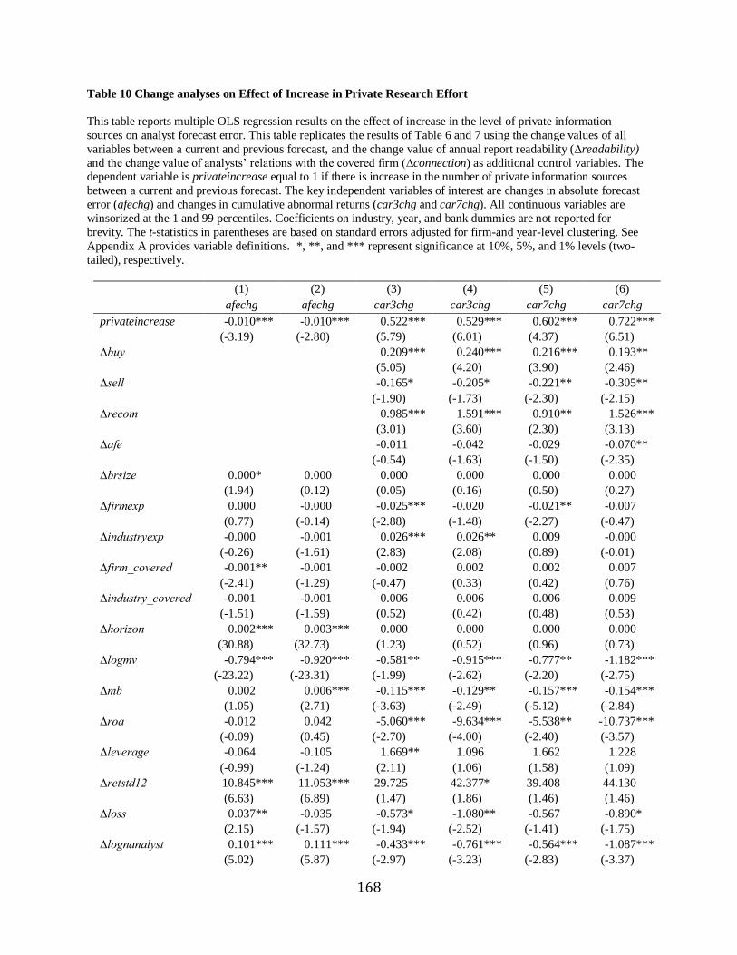
168

Table 10 Change analyses on Effect of Increase in Private Research Effort

This table reports multiple OLS regression results on the effect of increase in the level of private information

sources on analyst forecast error. This table replicates the results of Table 6 and 7 using the change values of all

variables between a current and previous forecast, and the change value of annual report readability (∆readability)

and the change value of analysts’ relations with the covered firm (∆connection) as additional control variables. The dependent variable is privateincrease equal to 1 if there is increase in the number of private information sources

between a current and previous forecast. The key independent variables of interest are changes in absolute forecast

error (afechg) and changes in cumulative abnormal returns (car3chg and car7chg). All continuous variables are

winsorized at the 1 and 99 percentiles. Coefficients on industry, year, and bank dummies are not reported for

brevity. The t-statistics in parentheses are based on standard errors adjusted for firm-and year-level clustering. See

Appendix A provides variable definitions. *, **, and *** represent significance at 10%, 5%, and 1% levels (two-

tailed), respectively.

(1) (2) (3) (4) (5) (6)

afechg afechg car3chg car3chg car7chg car7chg

privateincrease -0.010*** -0.010*** 0.522*** 0.529*** 0.602*** 0.722***

(-3.19) (-2.80) (5.79) (6.01) (4.37) (6.51)

∆buy 0.209*** 0.240*** 0.216*** 0.193**

(5.05) (4.20) (3.90) (2.46)

∆sell -0.165* -0.205* -0.221** -0.305**

(-1.90) (-1.73) (-2.30) (-2.15)

∆recom 0.985*** 1.591*** 0.910** 1.526***

(3.01) (3.60) (2.30) (3.13)

∆afe -0.011 -0.042 -0.029 -0.070**

(-0.54) (-1.63) (-1.50) (-2.35)

∆brsize 0.000* 0.000 0.000 0.000 0.000 0.000

(1.94) (0.12) (0.05) (0.16) (0.50) (0.27)

∆firmexp 0.000 -0.000 -0.025*** -0.020 -0.021** -0.007

(0.77) (-0.14) (-2.88) (-1.48) (-2.27) (-0.47)

∆industryexp -0.000 -0.001 0.026*** 0.026** 0.009 -0.000

(-0.26) (-1.61) (2.83) (2.08) (0.89) (-0.01)

∆firm_covered -0.001** -0.001 -0.002 0.002 0.002 0.007

(-2.41) (-1.29) (-0.47) (0.33) (0.42) (0.76)

∆industry_covered -0.001 -0.001 0.006 0.006 0.006 0.009

(-1.51) (-1.59) (0.52) (0.42) (0.48) (0.53)

∆horizon 0.002*** 0.003*** 0.000 0.000 0.000 0.000

(30.88) (32.73) (1.23) (0.52) (0.96) (0.73)

∆logmv -0.794*** -0.920*** -0.581** -0.915*** -0.777** -1.182***

(-23.22) (-23.31) (-1.99) (-2.62) (-2.20) (-2.75)

∆mb 0.002 0.006*** -0.115*** -0.129** -0.157*** -0.154***

(1.05) (2.71) (-3.63) (-2.49) (-5.12) (-2.84)

∆roa -0.012 0.042 -5.060*** -9.634*** -5.538** -10.737***

(-0.09) (0.45) (-2.70) (-4.00) (-2.40) (-3.57)

∆leverage -0.064 -0.105 1.669** 1.096 1.662 1.228

(-0.99) (-1.24) (2.11) (1.06) (1.58) (1.09)

∆retstd12 10.845*** 11.053*** 29.725 42.377* 39.408 44.130

(6.63) (6.89) (1.47) (1.86) (1.46) (1.46)

∆loss 0.037** -0.035 -0.573* -1.080** -0.567 -0.890*

(2.15) (-1.57) (-1.94) (-2.52) (-1.41) (-1.75)

∆lognanalyst 0.101*** 0.111*** -0.433*** -0.761*** -0.564*** -1.087***

(5.02) (5.87) (-2.97) (-3.23) (-2.83) (-3.37)

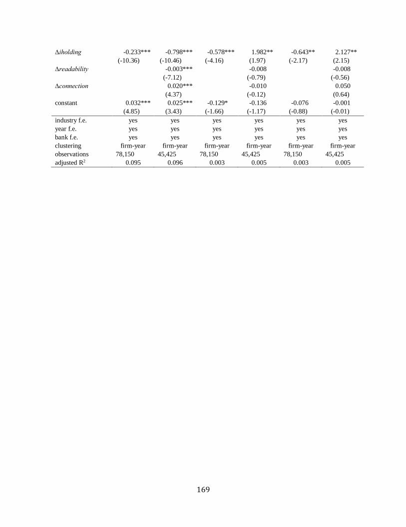
169

∆iholding -0.233*** -0.798*** -0.578*** 1.982** -0.643** 2.127**

(-10.36) (-10.46) (-4.16) (1.97) (-2.17) (2.15)

∆readability -0.003*** -0.008 -0.008

(-7.12) (-0.79) (-0.56)

∆connection 0.020*** -0.010 0.050

(4.37) (-0.12) (0.64)

constant 0.032*** 0.025*** -0.129* -0.136 -0.076 -0.001

(4.85) (3.43) (-1.66) (-1.17) (-0.88) (-0.01)

industry f.e. yes yes yes yes yes yes

year f.e. yes yes yes yes yes yes

bank f.e. yes yes yes yes yes yes

clustering firm-year firm-year firm-year firm-year firm-year firm-year

observations 78,150 45,425 78,150 45,425 78,150 45,425

adjusted R2 0.095 0.096 0.003 0.005 0.003 0.005

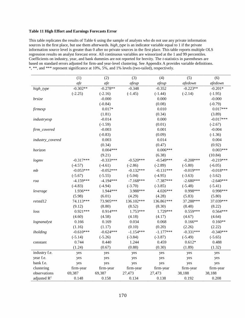
170

Table 11 High Effort and Earnings Forecasts Error

This table replicates the results of Table 6 using the sample of analysts who do not use any private information

sources in the first place, but use them afterwards. high_type is an indicator variable equal to 1 if the private

information source level is greater than 0 after no private sources in the first place. This table reports multiple OLS

regression results on analyst forecast error. All continuous variables are winsorized at the 1 and 99 percentiles. Coefficients on industry, year, and bank dummies are not reported for brevity. The t-statistics in parentheses are

based on standard errors adjusted for firm-and year-level clustering. See Appendix A provides variable definitions.

*, **, and *** represent significance at 10%, 5%, and 1% levels (two-tailed), respectively.

(1) (2) (3) (4) (5) (6)

afe afe afeup afeup afedown afedown

high_type -0.302** -0.278** -0.348 -0.352 -0.223** -0.201*

(-2.25) (-2.16) (-1.45) (-1.44) (-2.14) (-1.95)

brsize -0.000 0.000 -0.000

(-0.84) (0.08) (-0.79)

firmexp 0.017* 0.010 0.017***

(1.81) (0.34) (3.89)

industryexp -0.014 0.000 -0.017***

(-1.59) (0.01) (-2.67)

firm_covered -0.003 0.001 -0.004

(-0.83) (0.09) (-1.36)

industry_covered 0.003 0.014 0.004

(0.34) (0.47) (0.92)

horizon 0.004*** 0.006*** 0.003***

(9.21) (6.38) (10.84)

logmv -0.317*** -0.333*** -0.520*** -0.549*** -0.208*** -0.219***

(-4.57) (-4.61) (-2.86) (-2.89) (-5.80) (-6.05)

mb -0.053*** -0.052*** -0.132*** -0.131*** -0.019*** -0.018***

(-5.67) (-5.55) (-5.04) (-4.95) (-3.63) (-3.62)

roa -4.159*** -4.194*** -7.168*** -7.387*** -2.680*** -2.640***

(-4.83) (-4.94) (-3.70) (-3.85) (-5.48) (-5.41)

leverage 1.936*** 1.944*** 3.988*** 4.026*** 0.998*** 0.998***

(5.98) (6.01) (4.29) (4.28) (5.83) (5.80)

retstd12 74.113*** 73.905*** 136.102*** 136.861*** 37.288*** 37.039***

(9.12) (8.80) (8.52) (8.30) (8.48) (8.22)

loss 0.921*** 0.914*** 1.753*** 1.729*** 0.559*** 0.564***

(4.60) (4.58) (4.18) (4.17) (4.67) (4.64)

lognanalyst 0.166 0.169 0.034 0.068 0.166** 0.160**

(1.16) (1.17) (0.10) (0.20) (2.26) (2.22)

iholding -0.610*** -0.624*** -1.154*** -1.177*** -0.331*** -0.340***

(-5.14) (-5.26) (-3.84) (-3.87) (-5.49) (-5.65)

constant 0.744 0.440 1.244 0.459 0.612* 0.488

(1.24) (0.67) (0.88) (0.30) (1.89) (1.32)

industry f.e. yes yes yes yes yes yes

year f.e. yes yes yes yes yes yes

bank f.e. yes yes yes yes yes yes

clustering firm-year firm-year firm-year firm-year firm-year firm-year

observations 69,387 69,387 27,473 27,473 38,188 38,188

adjusted R2 0.148 0.158 0.134 0.138 0.192 0.208

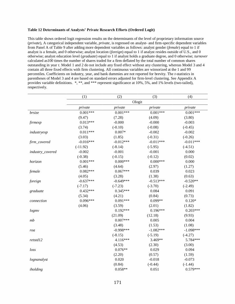
171

Table 12 Determinants of Analysts’ Private Research Efforts (Ordered Logit)

This table shows ordered logit regression results on the determinants of the level of proprietary information source

(private), A categorical independent variable, private, is regressed on analyst- and firm-specific dependent variables

from Panel A of Table 9 after adding more dependent variables as follows: analyst gender (female) equal to 1 if

analyst is a female, and 0 otherwise; analyst location (foreign) equal to 1 if analyst resides outside of U.S., and 0 otherwise; analyst education level (graduate) equal to 1 if analyst holds a graduate degree, and 0 otherwise; turnover

calculated as100 times the number of shares traded for a firm deflated by the total number of common shares

outstanding in year t. Model 1 and 2 do not include any fixed effect without any clustering, whereas Model 3 and 4

contain all three fixed effects with firm clustering. All continuous variables are winsorized at the 1 and 99

percentiles. Coefficients on industry, year, and bank dummies are not reported for brevity. The t-statistics in

parentheses of Model 3 and 4 are based on standard errors adjusted for firm-level clustering. See Appendix A

provides variable definitions. *, **, and *** represent significance at 10%, 5%, and 1% levels (two-tailed),

respectively.

(1) (2) (3) (4)

Ologit

private private private private

brsize 0.001*** 0.001*** 0.001*** 0.001***

(9.47) (7.28) (4.09) (3.80)

firmexp 0.013*** -0.000 -0.000 -0.003

(3.74) (-0.10) (-0.08) (-0.45)

industryexp 0.011*** 0.007* -0.002 -0.002

(3.03) (1.85) (-0.31) (-0.26)

firm_covered -0.016*** -0.012*** -0.011*** -0.011***

(-11.92) (-8.14) (-5.95) (-4.51)

industry_covered -0.002 -0.001 -0.001 0.000

(-0.38) (-0.15) (-0.12) (0.02)

horizon 0.001*** 0.000*** 0.000*** 0.000

(5.46) (4.64) (2.97) (1.27)

female 0.082*** 0.067*** 0.039 0.023

(4.05) (3.28) (1.38) (0.63)

foreign -0.637*** -0.649*** -0.513*** -0.520**

(-7.17) (-7.23) (-3.70) (-2.49)

graduate 0.432*** 0.345*** 0.084 0.091

(5.34) (4.21) (0.84) (0.73)

connection 0.096*** 0.091*** 0.099** 0.120*

(4.06) (3.59) (2.01) (1.82)

logmv 0.192*** 0.196*** 0.203***

(21.09) (12.18) (9.93)

mb 0.007*** 0.005 0.004

(3.48) (1.53) (1.08)

roa -0.998*** -1.082*** -1.098***

(-8.15) (-5.19) (-4.27)

retstd12 4.116*** 3.469** 5.784***

(4.53) (2.30) (3.00)

loss 0.076** 0.029 0.094

(2.20) (0.57) (1.59)

lognanalyst 0.020 -0.018 -0.073

(0.84) (-0.44) (-1.44)

iholding 0.058** 0.051 0.579***

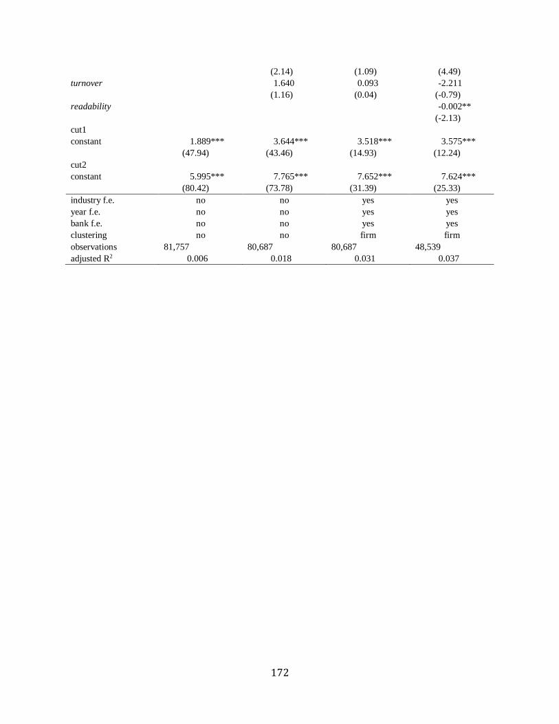
172

(2.14) (1.09) (4.49)

turnover 1.640 0.093 -2.211

(1.16) (0.04) (-0.79)

readability -0.002**

(-2.13)

cut1

constant 1.889*** 3.644*** 3.518*** 3.575***

(47.94) (43.46) (14.93) (12.24)

cut2

constant 5.995*** 7.765*** 7.652*** 7.624***

(80.42) (73.78) (31.39) (25.33)

industry f.e. no no yes yes

year f.e. no no yes yes

bank f.e. no no yes yes

clustering no no firm firm

observations 81,757 80,687 80,687 48,539

adjusted R2 0.006 0.018 0.031 0.037

173

Conclusion

This dissertation includes three different studies on the properties of analysts’ research

reports and firms’ annual reports.

Based on textual analysis of 351,629 analyst reports for US firms over 2000-2014, the

first essay investigates the determinants and consequences of analysts’ research report length.

Previous literature finds that management tends to write a longer annual report to hide/obfuscate

bad news. On the contrary, using textual analysis, I find that analysts tend to write a longer

analyst report to provide, not hide, more information to their investors, especially, when they

write stock recommendation upgrades which are perceived to be less credible than stock

recommendation downgrades. Previous studies argue that analysts tend to revise their

recommendation upward or at least maintain it, not revise downward due to keeping a good

relationship with management for private information and/or their conflict of interest. By

counting the number of pages in analyst research reports, I provide the first empirical evidence of

a stark contrast between a longer analyst report and a longer annual report.

Based on textual analysis of 81,826 10-Ks filed to the Securities and Exchange

Commission (SEC) by U.S. firms during 1998-2013, the second essay documents the positive

relationship of environmental disclosure with litigation risk which is another bad news. The

essay also finds that environmental disclosure is mean reverting since bad news is more likely to

be concealed relative to good news. Additionally, the essay shows that negative environmental

information is disclosed more than positive environmental information in 10-Ks. Overall, the

results identify disclosed environmental information as bad news that managers tend to hoard

inside their firm. If environmental disclosure is negative news, then it is expected that the stock

market negatively reacts to it around a 10-K filing date. The essay confirms this by documenting

174

a significantly negative association of environmental disclosure with cumulative abnormal

returns two days before and after the filing date. To the extent that disclosed environmental

information in 10-Ks is bad news, I am able to investigate the effect of environmental disclosure

on the future crash risk based on managers’ bad-news-hoarding hypothesis. I provide empirical

evidence that a firm with more environmental disclosure is less likely to experience major stock

price drops in the future because of less of the managers’ bad news hoarding tendency. The logit

regression shows that a one standard deviation increase of environmental disclosure reduces the

odds of a future crash risk by 10%, holding everything else constant. Further, using two

exogenous shocks as an instrumental variable, I identify a potential causality, over and above

mitigating potential endogeneity issues. Overall, the results are consistent with the idea that firms

benefit from non-financial information disclosure.

Using a pattern search algorithm (i.e., regular expression) on the headlines of 81,762

forecasts during 2000-2014, the third essay examines the relative value of private and public

information sources in analysts’ earnings forecasts for U.S. firms. As an information

intermediary, analysts access a private and/or public information source of a firm to make

forecasts for investors. Previous studies consistently find a higher accuracy of forecasts made

based on private information sources. Two sources, however, might equally be useful for

analysts to reduce forecast error. The essay finds no significant difference between a single

private and a single public information source in terms of analysts’ earnings forecast accuracy,

but an additional private information source might cause an increase in forecast accuracy. Given

that an additional private source requires more efforts by analysts even without information

advantage, investors highly appreciate the efforts by more strongly reacting to forecasts

containing the private information. This new perspective makes the essay to be differentiated

175

from previous literature supporting analysts’ information advantage hypothesis. Further analysis

shows that the combination of one management and one non-management private information

source tends to produce the highest forecast accuracy and the strongest market reaction.

Overall, three essays document that the stock market favorably reacts to the forecast

credibility-enhancing effort and the private information source-accessing effort by analysts. The

essay also shows that environmental disclosure in firms’ annual reports plays a role in reducing

the probability of future stock price crash risk.