ORIGINAL PAPER

The influence of DC stray current on pipeline corrosion

Gan Cui1 • Zi-Li Li1 • Chao Yang1 • Meng Wang1

Received: 4 February 2015 / Published online: 25 November 2015

� The Author(s) 2015. This article is published with open access at Springerlink.com

Abstract DC stray current can cause severe corrosion on

buried pipelines. In this study, firstly, we deduced the

equation of DC stray current interference on pipelines.

Next, the cathode boundary condition was discretized with

pipe elements, and corresponding experiments were

designed to validate the mathematical model. Finally, the

numerical simulation program BEASY was used to study

the corrosion effect of DC stray current that an auxiliary

anode bed generated in an impressed current cathodic

protection system. The effects of crossing angle, crossing

distance, distance of the two pipelines, anode output cur-

rent, depth, and soil resistivity were investigated. Our

results indicate that pipeline crossing substantially affects

the corrosion potential of both protected and unprotected

pipelines. Pipeline crossing angles, crossing distances, and

anode depths, our results suggest, have no significant

influence. Decreasing anode output current or soil resis-

tivity reduces pipeline corrosion gradually. A reduction of

corrosion also occurs when the distance between two par-

allel pipelines increases.

Keywords DC stray current � BEASY � Numerical

simulation � DC interference corrosion

1 Introduction

Stray current refers to the current that flows elsewhere

rather than along the intended current path. It is an

important cause of corrosion and leakage of underground

metal pipelines (Li et al. 2010; Guo et al. 2015). Stray

current corrosion is essentially electrochemical corrosion

(Bertolini et al. 2007). Because of the high electrical

conductivity of buried steel pipelines, potential differences

with the less conductive environment are formed when

stray current flows through the pipe (Brichau et al. 1996)

effectively creating a corrosion cell. The corrosion caused

by stray current is more serious than soil corrosion under

normal conditions (the potential difference of soil corro-

sion is only about 0.35 V without stray current, but the

pipe-to-soil potential can be as high as 8–9 V when a stray

current exists) (Brichau et al. 1996). The stray current has a

great effect on corrosion, and so affects the service life and

safe use of buried pipelines (Ding et al. 2010). Therefore, it

is important to better understand stray current corrosion.

There are three types of stray currents: direction current

(DC), alternating current (AC), and natural telluric current

in the earth. Among these, the DC stray current causes

most damage to a buried pipeline (Gao et al. 2010). The

DC stray current mainly originates from DC electrified

railways, DC electrolytic equipment grounding electrodes,

and the anode bed of cathodic protection systems (Wang

et al. 2010).

Numerical methods have been shown to be powerful

tools to analyze corrosion problems in the last two decades.

Numerical methods used for corrosion studies include the

finite difference method (FDM), the finite element method

(FEM) (Xu and Cheng 2013), and the boundary element

method (BEM) (Metwally et al. 2007; Boumaiza and Aour

2014; Bordon et al. 2014). The BEM was applied to model

& Zi-Li Li

cygcx@163.com

Gan Cui

chennacuigan@163.com

1 College of Pipeline and Civil Engineering, China University

of Petroleum (East China), Qingdao 266580, Shandong,

China

Edited by Yan-Hua Sun

123

Pet. Sci. (2016) 13:135–145

DOI 10.1007/s12182-015-0064-3

cathodic protection systems in the early 1980s (Wrobel and

Miltiadou 2004; DeGiorgi and Wimmer 2005; Lacerda

et al. 2007; Abootalebi et al. 2010; Lan et al. 2012; Liu

et al. 2013). Compared with FDM and FEM, BEM requires

the meshing of the boundary only. As a result, BEM needs

fewer equations resulting in a smaller matrix size than

FEM and can solve both finite and infinite domain prob-

lems (Jia et al. 2004; Parvanova et al. 2014). Last but not

least, the BEM has been specifically developed to calculate

the DC stray current induced in pipeline networks by

electric railways and can model the soil and the entire

traction system consisting of rails, traction stations, over-

head wires, and trains (Bortels et al. 2007; Poljak et al.

2010).

In this paper, the BEM is carried out to determine the

effect of DC interference corrosion on neighboring

pipelines (crossing or parallel with the cathodic protection

pipeline). It focuses on the DC current produced by the

auxiliary anode of the impressed current cathodic protec-

tion system.

2 Mathematical model

2.1 Governing equation

Some simplifications and assumptions are made here: the

solution around the pipeline is uniform and electroneutral,

and there is no concentration gradient in the solution.

Based on the above assumption and Ohm’s law, the

current density i can be expressed as follows (Metwally

et al. 2008):

i ¼ ree; ð1Þ

where re is the electrical conductivity of soil in S/m; i is

the current density in mA/m2; and e is the electric field in

V/m. Then, the static form of the equation of continuity can

be given as

ri ¼ rðreeÞ ¼ 0: ð2Þ

Under static conditions, the electric potential is defined

by the following equivalent equation:

r/ ¼ e: ð3Þ

Consequently, the governing equation for the electric

potential is the Laplace equation (Thamita 2012):

D/ ¼ 0: ð4Þ

2.2 Boundary conditions

Boundary conditions can be divided into the anode

boundary condition, the cathode boundary condition, and

the insulation boundary condition.

2.2.1 Anode and insulation boundary conditions

In this simulation, an impressed current cathodic protection

system is used and it is assumed that the output current of

the auxiliary anode is constant. Thus, the anode boundary

condition can be described as (Lan et al. 2012)

I ¼ I0: ð5Þ

The insulation boundary condition can be described as

o/on

¼ 0: ð6Þ

2.2.2 Cathode boundary condition

On the surface of the cathode, many complex electro-

chemical reactions occur. Polarization is one such conse-

quence of these reactions. The polarization data will be

used as the cathode boundary.

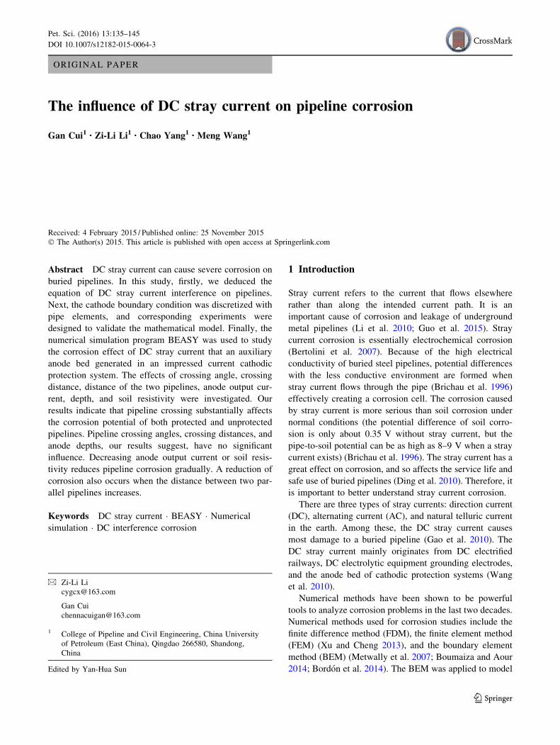
The polarization curve of steel was measured in the soil

environment using a conventional three-electrode cell

assembly. Rectangular platinum shapes were used as the

counter electrode and a saturated copper sulfate electrode

as reference. The working electrode was a cuboid, and its

material was Q235 steel. The steel electrode was embedded

in epoxy resin so that only a 1-cm2 area of the cuboid was

exposed to the soil. Before the experiment, the working

electrode was polished gradually using 600–1200 grid,

waterproof abrasive paper. It was then washed with dis-

tilled water, degreased with acetone, and washed with

ethanol. Finally, it was dried in an unheated air stream.

Electrochemical measurements were carried out using

electrochemical workstation Parstat 2273, which was spe-

cially designed for the study of the electrochemical cor-

rosion behavior. It can be used to test the open circuit

potential, electrochemical impedance spectroscopy (EIS),

Tafel polarization curve, cyclic voltammograms, etc. In

this paper, the Tafel curve was tested, and the polarization

measurement involved a scan starting from -400 to

-1200 mV at a scan rate of 0.3 mV/s.

The polarization curve is used as the cathode boundary

condition, but it is a nonlinear curve, so we have to use

polarization data in a piecewise linear interpolation

approach (Abootalebi et al. 2010; Liang et al. 2011; Liu

et al. 2013; Li et al. 2013). The polarization curve is shown

in Fig. 1, and we present it as a piecewise linear curve.

2.3 Boundary element method (BEM)

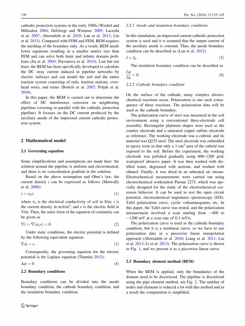
When the BEM is applied, only the boundaries of the

domain need to be discretized. The pipeline is discretized

using the pipe element method, see Fig. 2. The number of

nodes and elements is reduced a lot with this method and as

a result the computation is simplified.

136 Pet. Sci. (2016) 13:135–145

123

It should be noted that certain conditions need to be

met to use the pipe element method (Meng et al. 1998).

(1) The geometry of the protected body needs to be

suitable for cylinder unit subdivision. (2) The potential

everywhere on the same cylinder unit is considered

constant.

It is known that the fundamental solution of the

boundary integral equation is 14pr. Here ‘‘r’’ refers to the

distance between the boundary node and the source node.

Therefore, the integration will become a singularity when

the boundary node coincides with the source node.

2.3.1 Computation of the nonsingular coefficient

Based on the pipe element method above together with the

standard BEM formula, to make the boundaries discrete,

the coefficient matrix of each element is obtained by

integral transformation (Brichau and Deconinck 1994).

Gi;jmðtÞ ¼ 4RL

4pJj j/mðtÞ

4KðkÞ½ðRþ BÞ2 þ ðLt � ZrnÞ2�1=2

; ð7Þ

Hi;jmðtÞ ¼ Jj j/mðtÞ�RL

½ðRþ BÞ2 þ ðLt � ZrnÞ2�1=2ðLt � ZrnÞEðkÞ

p½ðR� BÞ2 þ ðLt � ZrnÞ2�2:

ð8Þ

In Eqs. (7) and (8), i = j. K(k) is the elliptic integral of

the first kind, while E(k) is the elliptic integral of the

second kind; J and B are the results of the coordinate

transformation; t is the local coordinate; and Zrn is the third

coordinate of the last pipe element node.

2.3.2 Computation of the singular coefficient

For the semi-infinite region (Wu 2008),

Hii ¼ �X

Hij; i 6¼ j: ð9Þ

The analytical method to solve Gii is

Gii ¼L

2p1� ln

L

16r

� �� �: ð10Þ

Finally, the standard BEM formula is represented by a

numerical integral, with the result

Gf g � Qf g ¼ Hf g � /� gðQÞf g: ð11Þ

3 Experimental

To validate the mathematical model, related experiments

were carried out in a controlled laboratory environment.

3.1 Experimental design

An experimental box was made of wood, 8000 mm 9

6000 mm 9 1500 mm (length 9 width 9 height), covered

0 20 40 60 80 100 120 140–1400

–1200

–1000

–800

–600

–400

Pot

entia

l E, m

V

Current density i, mA/m2

0 20 40 60 80 100 120 140–1400

–1200

–1000

–800

–600

–400

Current density i, mA/m2

Pot

entia

l E, m

V

a b

Fig. 1 The polarization curve. a Experimental polarization curve. b Piecewise linear polarization curve

A B C D E F

O Z

r

θ

Fig. 2 Pipe surface discretization

Pet. Sci. (2016) 13:135–145 137

123

with an insulating board. We also placed a PVC board under

it and around it. Two steel pipes were buried inside the box:

the protected pipe and the DC-interfered pipe. The parame-

ters of the protected pipe were material Q235 steel—no

coating, outside diameter 20 mm, wall thickness 3 mm,

length 6000 mm, and depth 1 m. The parameters of the DC-

interfered pipe were material Q235—no coating, outside

diameter 20 mm, wall thickness 3 mm, length 4000 mm,

depth 0.5 m. The parameters of the auxiliary anode with a

treated cylindrical surface were diameter 0.03 m, length

0.1 m, depth 1 m, distance from the pipe 0.3 m, no fillers,

and the output current 1 mA.

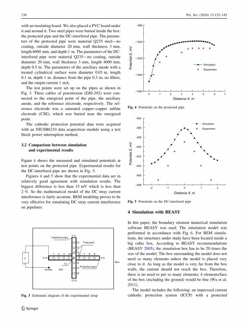
The test points were set up on the pipes as shown in

Fig. 3. Three cables of potentiostat (DJS-292) were con-

nected to the energized point of the pipe, the auxiliary

anode, and the reference electrode, respectively. The ref-

erence electrode was a saturated copper–copper sulfate

electrode (CSE), which was buried near the energized

point.

The cathodic protection potential data were acquired

with an NIUSB6210 data acquisition module using a test

block power interruption method.

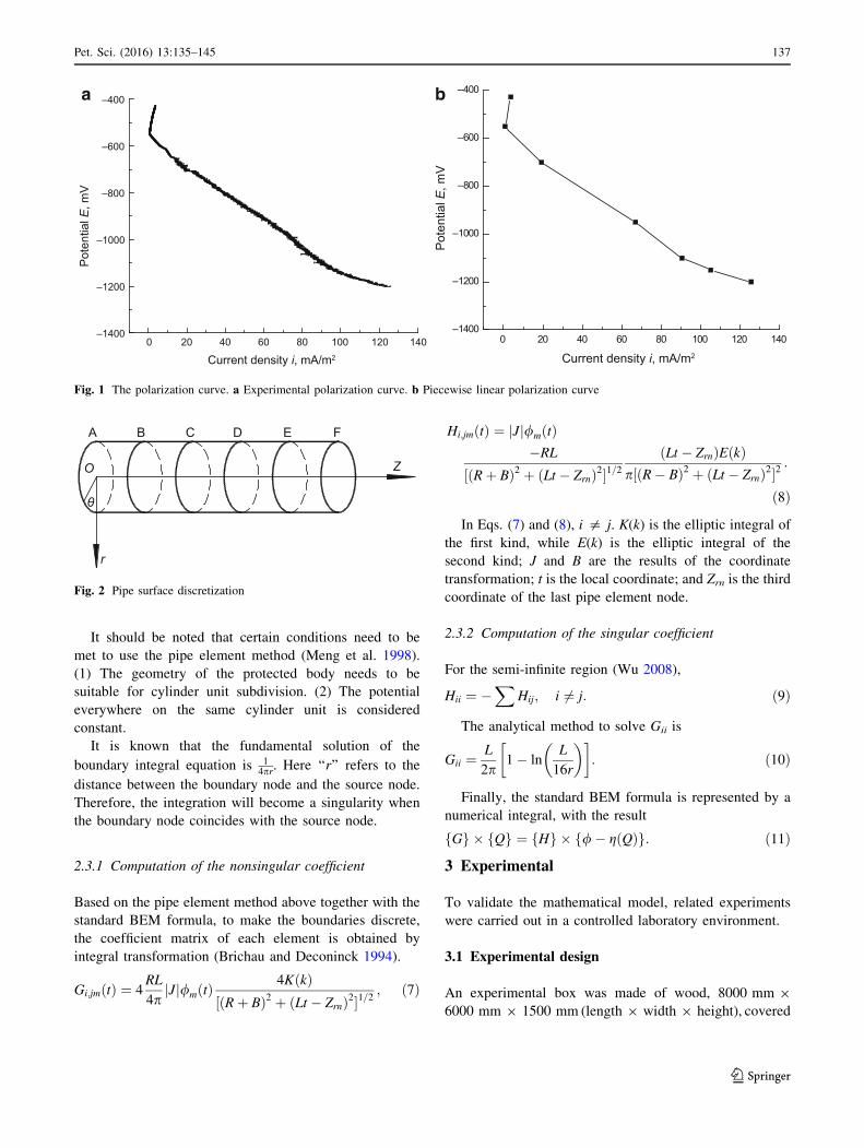
3.2 Comparison between simulation

and experimental results

Figure 4 shows the measured and simulated potentials at

test points on the protected pipe. Experimental results for

the DC-interfered pipe are shown in Fig. 5.

Figures 4 and 5 show that the experimental data are in

relatively good agreement with simulation results. The

biggest difference is less than 15 mV which is less than

2 %. So the mathematical model of the DC stray current

interference is fairly accurate. BEM modeling proves to be

very effective for simulating DC stray current interference

on pipelines.

4 Simulation with BEASY

In this paper, the boundary element numerical simulation

software BEASY was used. The simulation model was

performed in accordance with Fig. 6. For BEM simula-

tions, the structures under study have been located inside a

big cubic box. According to BEASY recommendations

(BEASY 2005), the simulation box has to be 20 times the

size of the model. The box surrounding the model does not

need so many elements unless the model is placed very

close to it. As long as the model is very far from the box

walls, the current should not reach the box. Therefore,

there is no need to put so many elements; 4 elements/face

of the box (including the ground) would be fine (Wu et al.

2011).

The model includes the following: an impressed current

cathodic protection system (ICCP) with a protected

Box

–2 m

2 m

Test point

6 m

Soil

+

−

V 0 m

Anode

Interfered pipe

Protected pipe

1 63 42 5

14

8 9

10

11

15

712

16

13

Fig. 3 Schematic diagram of the experimental setup

0 1 2 3 4 5 6 7–1060

–1040

–1020

–1000

–980

Distance X, m

Simulation

ExperimentPot

entia

l E, m

V

Fig. 4 Potentials on the protected pipe

–2 –1 0 1 2─608

–606

–604

–602

–600

–598

–596

–594

Simulation

Experiment

Distance X, m

Pot

entia

l E, m

V

Fig. 5 Potentials on the DC-interfered pipe

138 Pet. Sci. (2016) 13:135–145

123

pipeline (pipeline 1). Pipeline 2 is located near pipeline 1

and has no applied cathodic protection. Therefore, part of

the cathodic protection current that the auxiliary anode

carries to pipeline 1 will flow into pipeline 2 as stray

current and affects the corrosion of pipeline 2—see Fig. 6.

The origin is chosen as the intersection between the two

pipelines, and the parameters in the model are set as follows:

Pipeline 1: Two endpoint coordinates are (-800 m, 0 m,

-4 m) and (800 m, 0 m, -4 m), diameter is 0.762 m, and

the material is Q235; Pipeline 2: Two endpoints coordinate

are (0 m, -800 m, -2 m) and (0 m, 800 m, -2 m), diam-

eter is 0.4064 m, and the material is Q235. The coating on

both pipelines is assumed to have 5 %damage. The auxiliary

anode which is vertically buried has the following parame-

ters: two endpoint coordinates (-800 m, -100 m, -1 m)

and (-800 m, -100 m, -6 m), diameter 0.1 m, and con-

stant current 2400 mA. Soil conductivity in the area of the

buried pipelines is 0.005 S/m. It should be noted that all

simulated potential data below are with respect to the satu-

rated copper sulfate reference electrode.

5 Results and discussion

5.1 Effect of pipeline crossing

Considering the situation of two pipelines intersecting at an

angle of 90�, the setting of each parameter is the same as in

Sect. 4. Both potential distribution and current density

distribution of pipeline 2 are obtained by simulation, and

the results are shown in Fig. 7.

As shown in Fig. 7a, the change in the potential distri-

bution of pipeline 2 is very large where the two pipelines

intersect. The corrosion potential near the intersection is

higher than the self-corrosion potential, and the potential of

the intersection is then most positive. The potential at each

end of the pipeline is lower than the pipeline self-corrosion

potential. Considering the stray corrosion current density in

Fig. 7b, in this section, the current density is positive which

means that the current flows out of the pipeline. Therefore,

that section of the pipeline becomes an anode, and its

potential is higher than the self-corrosion potential which

makes corrosion more severe. The section that shows a

negative current density has current flowing into the

pipeline—in other words, it becomes a cathode. Its

potential is lower than the self-corrosion potential. It

receives some cathodic protection which reduces corrosion.

5.2 Effect of pipeline crossing on the cathodic

protection potential distribution

The following assumptions are made: Pipeline 2 also receives

applied impressed current cathodic protection. The coordi-

nates of the auxiliary anode of pipeline 2 are (100 m,-800 m,

-1 m) and (100 m, -800 m, -6 m). The current is also

2400 mA, and the rest of the parameters remain unchanged.

The distribution of the cathodic protection potential and cur-

rent density of two pipelines are shown in Fig. 8.

According to Fig. 8, a large change of the cathodic

protection potentials occurs near the intersection between

the two pipelines. There is a clear potential increase with

the maximum at the intersection. The current density,

TRU supplying constant current

ICCP anode

Pipe 1

Pipe 2

Stray currents

Current flowingin the return pathcircuit

(–800 m, 0 m, –4 m) (800 m, 0 m, –4 m)

(0 m, –800 m, –2 m)

(0 m, 800 m, –2 m)

Fig. 6 Schematic of the DC interference model. The anode ground bed produces the DC stray current. Pipeline 2 is rotated anticlockwise to

study four different crossing angles (30�, 45�, 60�, and 90�)

Pet. Sci. (2016) 13:135–145 139

123

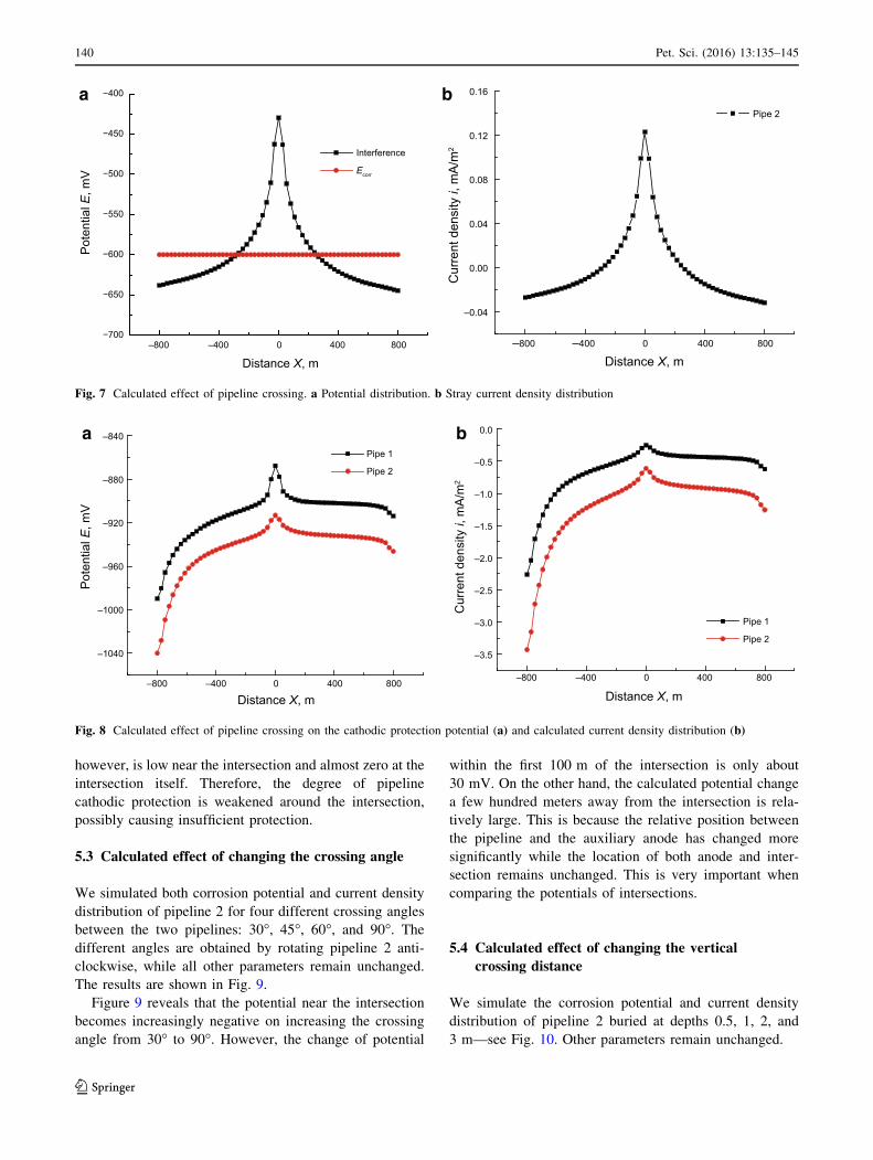
however, is low near the intersection and almost zero at the

intersection itself. Therefore, the degree of pipeline

cathodic protection is weakened around the intersection,

possibly causing insufficient protection.

5.3 Calculated effect of changing the crossing angle

We simulated both corrosion potential and current density

distribution of pipeline 2 for four different crossing angles

between the two pipelines: 30�, 45�, 60�, and 90�. Thedifferent angles are obtained by rotating pipeline 2 anti-

clockwise, while all other parameters remain unchanged.

The results are shown in Fig. 9.

Figure 9 reveals that the potential near the intersection

becomes increasingly negative on increasing the crossing

angle from 30� to 90�. However, the change of potential

within the first 100 m of the intersection is only about

30 mV. On the other hand, the calculated potential change

a few hundred meters away from the intersection is rela-

tively large. This is because the relative position between

the pipeline and the auxiliary anode has changed more

significantly while the location of both anode and inter-

section remains unchanged. This is very important when

comparing the potentials of intersections.

5.4 Calculated effect of changing the vertical

crossing distance

We simulate the corrosion potential and current density

distribution of pipeline 2 buried at depths 0.5, 1, 2, and

3 m—see Fig. 10. Other parameters remain unchanged.

–800 –400 0 400 800−700

−650

−600

−550

−500

−450

−400P

oten

tial E

, mV

Distance X, m

Interference

Ecorr

─800 ─400 0 400 800

–0.04

0.00

0.04

0.08

0.12

0.16

Cur

rent

den

sity

i, m

A/m

2

Distance X, m

Pipe 2

a b

Fig. 7 Calculated effect of pipeline crossing. a Potential distribution. b Stray current density distribution

–800 –400 0 400 800

–1040

–1000

–960

–920

–880

–840

Pote

ntia

l E, m

V

Distance X, m

Pipe 1

Pipe 2

–800 –400 0 400 800

–3.5

–3.0

–2.5

–2.0

–1.5

–1.0

–0.5

0.0

Cur

rent

den

sity

i, m

A/m

2

Distance X, m

Pipe 1

Pipe 2

a b

Fig. 8 Calculated effect of pipeline crossing on the cathodic protection potential (a) and calculated current density distribution (b)

140 Pet. Sci. (2016) 13:135–145

123

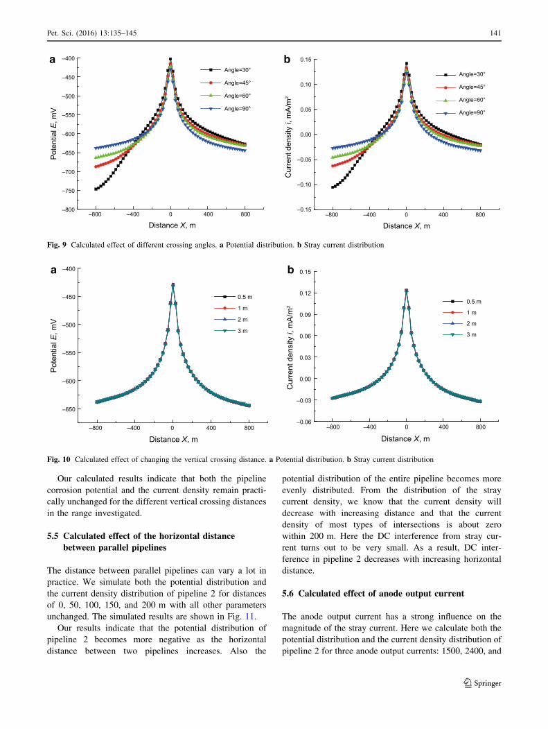
Our calculated results indicate that both the pipeline

corrosion potential and the current density remain practi-

cally unchanged for the different vertical crossing distances

in the range investigated.

5.5 Calculated effect of the horizontal distance

between parallel pipelines

The distance between parallel pipelines can vary a lot in

practice. We simulate both the potential distribution and

the current density distribution of pipeline 2 for distances

of 0, 50, 100, 150, and 200 m with all other parameters

unchanged. The simulated results are shown in Fig. 11.

Our results indicate that the potential distribution of

pipeline 2 becomes more negative as the horizontal

distance between two pipelines increases. Also the

potential distribution of the entire pipeline becomes more

evenly distributed. From the distribution of the stray

current density, we know that the current density will

decrease with increasing distance and that the current

density of most types of intersections is about zero

within 200 m. Here the DC interference from stray cur-

rent turns out to be very small. As a result, DC inter-

ference in pipeline 2 decreases with increasing horizontal

distance.

5.6 Calculated effect of anode output current

The anode output current has a strong influence on the

magnitude of the stray current. Here we calculate both the

potential distribution and the current density distribution of

pipeline 2 for three anode output currents: 1500, 2400, and

–800 –400 0 400 800–800

–750

–700

–650

–600

–550

–500

–450

–400

Distance X, m

Angle=30°

Angle=45°

Angle=60°

Angle=90°

Pot

entia

l E, m

V

–800 –400 0 400 800–0.15

–0.10

–0.05

0.00

0.05

0.10

0.15

Cur

rent

den

sity

i, m

A/m

2

Distance X, m

Angle=30°

Angle=45°

Angle=60°

Angle=90°

a b

Fig. 9 Calculated effect of different crossing angles. a Potential distribution. b Stray current distribution

–800 –400 0 400 800

–650

–600

–550

–500

–450

–400

Pot

entia

l E, m

V

0.5 m

1 m

2 m

3 m

Distance X, m

–800 –400 0 400 800–0.06

–0.03

0.00

0.03

0.06

0.09

0.12

0.15

Cur

rent

den

sity

i, m

A/m

2

Distance X, m

0.5 m

1 m

2 m

3 m

a b

Fig. 10 Calculated effect of changing the vertical crossing distance. a Potential distribution. b Stray current distribution

Pet. Sci. (2016) 13:135–145 141

123

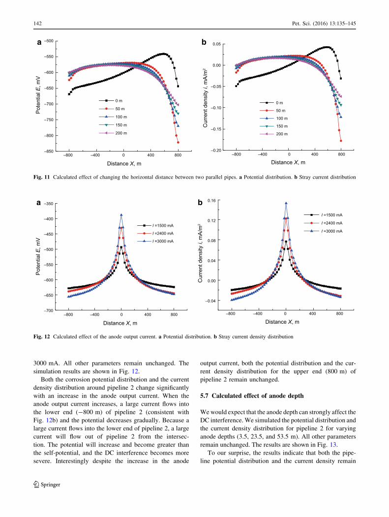
3000 mA. All other parameters remain unchanged. The

simulation results are shown in Fig. 12.

Both the corrosion potential distribution and the current

density distribution around pipeline 2 change significantly

with an increase in the anode output current. When the

anode output current increases, a large current flows into

the lower end (-800 m) of pipeline 2 (consistent with

Fig. 12b) and the potential decreases gradually. Because a

large current flows into the lower end of pipeline 2, a large

current will flow out of pipeline 2 from the intersec-

tion. The potential will increase and become greater than

the self-potential, and the DC interference becomes more

severe. Interestingly despite the increase in the anode

output current, both the potential distribution and the cur-

rent density distribution for the upper end (800 m) of

pipeline 2 remain unchanged.

5.7 Calculated effect of anode depth

Wewould expect that the anode depth can strongly affect the

DC interference.We simulated the potential distribution and

the current density distribution for pipeline 2 for varying

anode depths (3.5, 23.5, and 53.5 m). All other parameters

remain unchanged. The results are shown in Fig. 13.

To our surprise, the results indicate that both the pipe-

line potential distribution and the current density remain

–800 –400 0 400 800–850

–800

–750

–700

–650

–600

–550

–500P

oten

tial E

, mV

Distance X, m

0 m

50 m

100 m

150 m

200 m

–800 –400 0 400 800–0.20

–0.15

–0.10

–0.05

0.00

0.05

Cur

rent

den

sity

i, m

A/m

2

Distance X, m

0 m

50 m

100 m

150 m

200 m

a b

Fig. 11 Calculated effect of changing the horizontal distance between two parallel pipes. a Potential distribution. b Stray current distribution

–800 –400 0 400 800–700

–650

–600

–550

–500

–450

–400

–350

Pot

entia

l E, m

V

Distance X, m

I =1500 mA

I =2400 mA

I =3000 mA

–800 –400 0 400 800

–0.04

0.00

0.04

0.08

0.12

0.16C

urre

nt d

ensi

ty i,

mA

/m2

I =1500 mA

I =2400 mA

I =3000 mA

Distance X, m

a b

Fig. 12 Calculated effect of the anode output current. a Potential distribution. b Stray current density distribution

142 Pet. Sci. (2016) 13:135–145

123

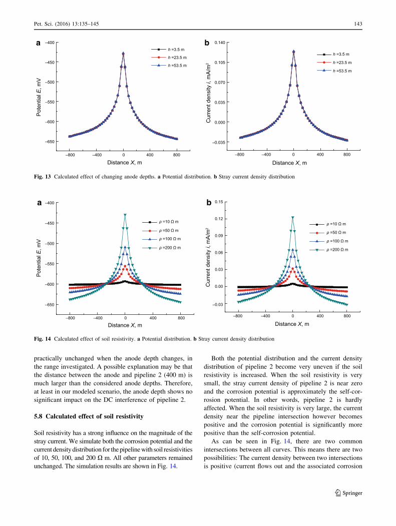
practically unchanged when the anode depth changes, in

the range investigated. A possible explanation may be that

the distance between the anode and pipeline 2 (400 m) is

much larger than the considered anode depths. Therefore,

at least in our modeled scenario, the anode depth shows no

significant impact on the DC interference of pipeline 2.

5.8 Calculated effect of soil resistivity

Soil resistivity has a strong influence on the magnitude of the

stray current. We simulate both the corrosion potential and the

current density distribution for thepipelinewith soil resistivities

of 10, 50, 100, and 200 X m. All other parameters remained

unchanged. The simulation results are shown in Fig. 14.

Both the potential distribution and the current density

distribution of pipeline 2 become very uneven if the soil

resistivity is increased. When the soil resistivity is very

small, the stray current density of pipeline 2 is near zero

and the corrosion potential is approximately the self-cor-

rosion potential. In other words, pipeline 2 is hardly

affected. When the soil resistivity is very large, the current

density near the pipeline intersection however becomes

positive and the corrosion potential is significantly more

positive than the self-corrosion potential.

As can be seen in Fig. 14, there are two common

intersections between all curves. This means there are two

possibilities: The current density between two intersections

is positive (current flows out and the associated corrosion

–800 –400 0 400 800

–650

–600

–550

–500

–450

–400P

oten

tial E

, mV

Distance X, m

h =3.5 m

h =23.5 m

h =53.5 m

–800 –400 0 400 800

–0.035

0.000

0.035

0.070

0.105

0.140

Cur

rent

den

sity

i, m

A/m

2

Distance X, m

h =3.5 m

h =23.5 m

h =53.5 m

a b

Fig. 13 Calculated effect of changing anode depths. a Potential distribution. b Stray current density distribution

–800 –400 0 400 800

–650

–600

–550

–500

–450

–400

ρ =10 Ω m

Pot

entia

l E, m

V

Distance X, m

ρ =50 Ω m

ρ =100 Ω m

ρ =200 Ω m

–800 –400 0 400 800

0.00

0.03

0.06

0.09

0.12

0.15

Cur

rent

den

sity

i, m

A/m

2

Distance X, m

ρ =10 Ω m

ρ =50 Ω m

ρ =100 Ω m

ρ =200 Ω m

–0.03

a b

Fig. 14 Calculated effect of soil resistivity. a Potential distribution. b Stray current density distribution

Pet. Sci. (2016) 13:135–145 143

123

of the pipeline is more severe) or the current density out-

side two intersections is negative (current flows in and the

pipeline has some cathodic protection).

As a consequence, the change of soil resistivity does not

result in the change of the location and length of affected

pipe sections. It only affects the degree of corrosion.

6 Conclusions

The following conclusions can be drawn based on our

experiments and simulation:

(1) The mathematical model of the DC stray current

interference in pipelines investigated in this paper is

accurate, and BEM is confirmed to simulate DC

stray current interference on pipelines very well.

(2) The potential distribution of the pipeline changes a

lot when the pipelines cross. The potential at the

intersection is about 200 mV higher than the self-

corrosion potential which renders the corrosion of

the pipeline in the intersection quite severe. The

potentials at the two ends are about 50 mV lower

than the self-corrosion potential. This part of the

pipeline appears to receive some cathodic protection.

(3) The variation of the pipeline crossing angle, vertical

crossing distance, and anode depth has little impact

on the potential and the current density distribution

of the DC-interfered pipeline.

(4) Upon increasing the horizontal distance between

parallel pipelines, the corrosion potential of the

affected section becomes negative, the potential

distribution becomes more uniform, and the degree

of the DC interference decreases.

(5) Upon increasing either the anode output current or

the soil resistivity, the corrosion potential of the DC-

interfered pipeline becomes very uneven. The cor-

rosion potential of the pipeline near the intersection

has a large positive offset, and pipeline corrosion

becomes worse. However, the corrosion potential

and the current density distribution at the far end

(800 m) of pipeline 2 remain unchanged after

increasing the anode output current. Change in

resistivity just changes the degree of corrosion of

the affected section but does not change the location

and length of the affected pipe sections.

Open Access This article is distributed under the terms of the Crea-

tive Commons Attribution 4.0 International License (http://creative

commons.org/licenses/by/4.0/), which permits unrestricted use,

distribution, and reproduction in any medium, provided you give

appropriate credit to the original author(s) and the source, provide a link

to the Creative Commons license, and indicate if changes were made.

References

Abootalebi O, Kermanpur A, Shishesaz MR, et al. Optimizing the

electrode position in sacrificial anode cathodic protection

systems using boundary element method. Corros Sci.

2010;52(3):678–87. doi:10.1016/j.corsci.2009.10.025.

BEASY software user guide, computational mechanics BEASY

Version 10. Southampton, UK, 2005. Available: http://www.

beasy.com.

Bertolini L, Carsana M, Pedeferri P. Corrosion behavior of steel in

concrete in the presence of stray current. Corros Sci.

2007;49(3):1056–68. doi:10.1016/j.corsci.2006.05.048.

Bordon JDR, Aznarez JJ, Maeso O. A 2D BEM–FEM approach for

time harmonic fluid–structure interaction analysis of thin elastic

bodies. Eng Anal Bound Elem. 2014;43(6):19–29. doi:10.1016/j.

enganabound.2014.03.004.

Bortels L, Dorochenko A, Bossche BV, et al. Three-dimensional

boundary element method and finite element method simulations

applied to stray current interference problems. A unique

coupling mechanism that takes the best of both methods.

Corrosion. 2007;63(6):561–76. doi:10.5006/1.3278407.

Boumaiza D, Aour B. On the efficiency of the iterative coupling

FEM–BEM for solving the elasto-plastic problems. Eng Struct.

2014;72(8):12–25. doi:10.1016/j.engstruct.2014.03.036.

Brichau F, Deconinck J. A numerical model for cathodic protection

of buried pipes. Corrosion. 1994;50(1):39–49. doi:10.5006/1.

3293492.

Brichau F, Deconinck J, Driesens T. Modeling of underground

cathodic protection stray currents. Corrosion. 1996;52(6):480–8.

doi:10.5006/1.3292137.

DeGiorgi VG, Wimmer SA. Geometric details and modeling accuracy

requirements for shipboard impressed current cathodic protec-

tion system modeling. Eng Anal Boundary Elem. 2005;29(1):

15–28. doi:10.1016/j.enganabound.2004.09.006.

Ding HT, Li LJ, Jiang MH, et al. Lab research of DC & AC stray

current for the failure effect of the gas pipelines buried

underground. Guizhou Chem Ind. 2010;35(5):9–12 (in Chinese).

Gao B, Shen LS, Meng XQ, et al. DC stray current corrosion and

protection of oil gas pipelines. Pipeline Technol Equip.

2010;4:42–3 (in Chinese).

Guo YB, Liu C, Wang DG, Liu SH. Effects of alternating current

interference on corrosion of X60 pipeline steel. Pet Sci.

2015;12(2):316–24. doi:10.1007/s12182-015-0022-0.

Jia JX, Song G, Atrens A, et al. Evaluation of the BEASY program

using linear and piecewise linear approaches for the boundary

conditions. Mater Corros. 2004;55(11):845–52. doi:10.1002/

maco.200403795.

Lacerda LAD, Silva JMD, Jose L. Dual boundary element formula-

tion for half-space cathodic protection analysis. Eng Anal Bound

Elem. 2007;31(6):559–67. doi:10.1016/j.enganabound.2006.10.

007.

Lan ZG, Wang XT, Hou BR, et al. Simulation of sacrificial anode

protection for steel platform using boundary element method.

Eng Anal Boundary Elem. 2012;36(5):903–6. doi:10.1016/j.

enganabound.2011.07.018.

Li YT, Wu MT, Zheng F, et al. Stray current monitoring for pipelines

and an application example in the Chuanxi gas field. Total

Corros Control. 2010;24(1):25–8 (in Chinese).

Li ZL, Cui G, Shang XB, et al. Defining cathodic protection potential

distribution of long distance pipelines with numerical simulation.

Corros Prot. 2013;34(6):468–71 (in Chinese).

Liang CH, Yuan CJ, Huang NB. Defining the voltage distribution of a

pipeline in frozen earth under cathodic protection with a

boundary element method. J Dalian Marit Univ. 2011;37(4):

109–16 (in Chinese).

144 Pet. Sci. (2016) 13:135–145

123

Liu C, Shankar A, Orazem ME, et al. Numerical simulations for

cathodic protection of pipelines. Undergr Pipeline Corros.

2014;63:85–126.

Liu GC, Sun W, Wang L, et al. Modeling cathodic shielding of

sacrificial anode cathodic protection systems in sea water. Mater

Corros. 2013;63(6):472–7. doi:10.1002/maco.201206726.

Meng XJ, Wu ZY, Liang XW, et al. Improvement of algorithms for a

regional cathodic protection model. J Chin Soc Corros Prot.

1998;9:221–6 (in Chinese).

Metwally IA, Al-Mandhari HM, Gastli A, et al. Factors affecting

cathodic-protection interference. Eng Anal Bound Elem.

2007;31(6):485–93. doi:10.1016/j.enganabound.2006.11.003.

Metwally IA, Al-Mandhari HM, Gastli A, et al. Stray currents of ESP

well casings. Eng Anal Bound Elem. 2008;32(1):32–40. doi:10.

1016/j.enganabound.2007.06.003.

Parvanova SL, Dineva PS, Manolis GD, et al. Dynamic response of a

solid with multiple inclusions under anti-plane strain conditions

by the BEM. Comput Struct. 2014;139(7):65–83. doi:10.1016/j.

compstruc.2014.04.002.

Poljak D, Sesnic S, Goic R. Analytical versus boundary element

modelling of horizontal ground electrode. Eng Anal Bound

Elem. 2010;34(4):307–14. doi:10.1016/j.enganabound.2009.10.

008.

Thamita SK. Modeling and simulation of galvanic corrosion pit as

a moving boundary problem. Comput Mater Sci. 2012;

65(12):269–75. doi:10.1016/j.commatsci.2012.07.029.

Wang Y, Yan YG, Dong CF, et al. Effect of stray current on corrosion

of Q235, 16Mn and X70 steels with damaged coating. Corros Sci

Prot Technol. 2010;22(2):117–9 (in Chinese).

Wrobel LC, Miltiadou P. Genetic algorithms for inverse cathodic

protection problems. Eng Anal Bound Elem. 2004;28(3):267–77.

doi:10.1016/S0955-7997(03)00057-2.

Wu HT. The application of boundary element method in heat transfer.

Beijing: National Defence Industry Press; 2008. p. 24–7 (in

Chinese).

Wu JH, Xing SH, Liang CH, et al. The influence of electrode position

and output current on the corrosion related electro-magnetic field

of ship. Adv Eng Softw. 2011;42(10):902–9. doi:10.1016/j.

advengsoft.2011.06.007.

Xu LY, Cheng YF. Development of a finite element model for

simulation and prediction of mechanoelectrochemical effect of

pipeline corrosion. Corros Sci. 2013;73(8):150–60. doi:10.1016/

j.corsci.2013.04.004.

Pet. Sci. (2016) 13:135–145 145

123