The Influence of End Conditions on Vortex Shedding from … · The Influence of End Conditions on Vortex Shedding from a Circular Cylinder in Sub-Critical Flow ... 2.2.4 Fast Fourier

The Influence of End Conditions on Vortex Shedding from a

Circular Cylinder in Sub-Critical Flow

by

Eric Khoury

A thesis submitted in conformity with the requirements

for the degree of Master of Applied Science in Engineering

Institute for Aerospace Studies

University of Toronto

© Copyright by Eric Khoury 2012

ii

The Influence of End Conditions on Vortex Shedding from a Circular

Cylinder in Sub-Critical Flow

Eric Khoury

Master of Applied Science in Engineering

Institute of Aerospace Studies

University of Toronto

2012

Abstract

The effect of end boundary conditions on the three-dimensionality of the vortex shedding from a

circular cylinder in sub-critical flow has been studied experimentally, with a focus on the unsteady

nature of the vortex filaments. Analysis of the near-wake of the cylinder was undertaken to

determine the dependency of the spanwise uniformity of the vortex shedding on the end conditions.

Flow visualization was performed downstream of the cylinder, and the temporal variation of the

vortex filament angle was observed. Vortex dislocations were found to occur in this Reynolds

Number regime regardless of the end boundary conditions. Having a cylinder bounded by two

elliptical leading edge geometry endplates at an L/D value of five yielded parallel shedding with a

reduction in the time-based variation of the vortex filament angle, and was shown to be the ideal end

conditions for modeling an infinite cylinder in a free-surface water channel.

iii

Acknowledgments

I would like to thank my supervisor Dr. Ekmekci for her guidance at my time at UTIAS. I would

also like to thank my research committee, Dr. Zingg, Dr. Lavoie, Dr. Steeves and Dr. Ekmekci for

their very useful advice throughout the entire thesis process. I also wish to thank all the students in

the office for creating a great work environment. Specifically I am very grateful for all the hours of

experimental setup help and explanation my lab mates Tayfun Aydin and Antrix Joshi gave me

during my time at UTIAS. Finally I wish to thank my family for all the support they have given me

during this process, if it was not for them I would not be in the position I am in today.

iv

Table of Contents

Contents

Acknowledgments.......................................................................................................................... iii

Table of Contents ........................................................................................................................... iv

List of Tables ................................................................................................................................. vi

List of Figures ............................................................................................................................... vii

Introduction .................................................................................................................................1 1

1.1 Motivation and Background ................................................................................................1

1.2 Literature Review.................................................................................................................2

1.2.1 Flow Past an Infinite Cylinder .................................................................................2

1.2.2 End Effects on the Spanwise Uniformity of the Cylinder Near Wake ....................4

Experimental Setup and Analysis Techniques ............................................................................9 2

2.1 Experimental Setup ..............................................................................................................9

2.1.1 Water Channel .........................................................................................................9

2.1.2 Test models ..............................................................................................................9

2.1.3 Particle Image Velocimetry ...................................................................................11

2.1.4 Constant Temperature Anemometry ......................................................................14

2.2 Analysis Techniques ..........................................................................................................16

2.2.1 Time-Averaged Recirculation Region ...................................................................16

2.2.2 Space-Time Plots ...................................................................................................17

2.2.3 Continuous Wavelet Transformation .....................................................................18

2.2.4 Fast Fourier Transform and Short-Time Fourier Transform .................................19

2.2.5 Time Evolution of Phase-Angle Difference Between Two Probes .......................20

v

Results .......................................................................................................................................27 3

3.1 Time-Averaged Characteristics of Vortex Shedding .........................................................27

3.2 Unsteady Nature of Vortex Filaments ...............................................................................29

3.2.1 Visualization of Vortex Filaments .........................................................................29

3.2.2 Effect of End Configuration on the Vortex Filament Orientation .........................31

3.2.3 Vortex Splitting ......................................................................................................34

Conclusion and Future Work ....................................................................................................60 4

Appendix A ....................................................................................................................................63

References ......................................................................................................................................66

vi

List of Tables

Table 1: Acquisition details for PIV measurements ........................................................................... 12

Table 2: Probe Characteristics ............................................................................................................ 15

Table 3: Error in calculated recirculation region as a function of Reynolds number ......................... 17

vii

List of Figures

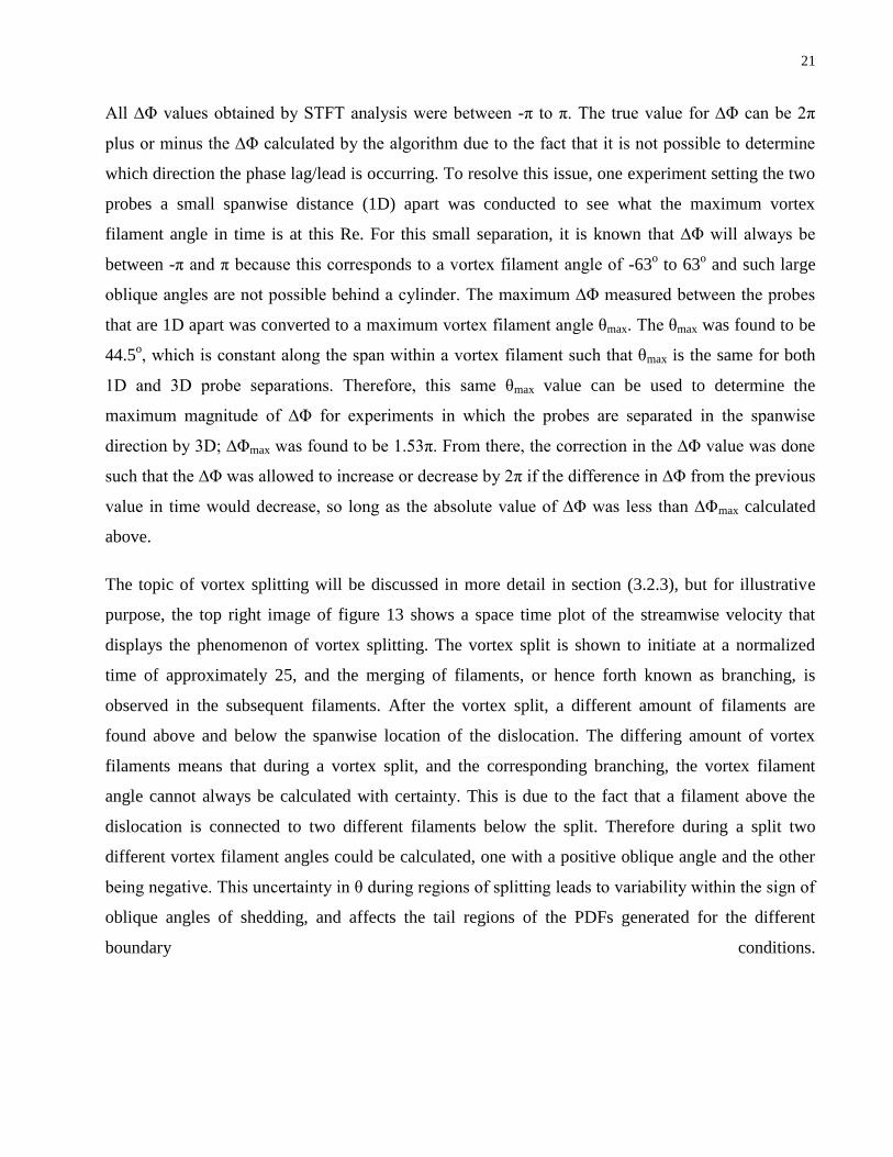
Figure 1: The various boundary conditions investigated. a) A cylinder bounded by the channel floor

and free-surface. b) A cylinder bounded by the channel floor and the channel cover. c) A cylinder

bounded by a sharp leading edge geometry endplate on the bottom and the free-surface on top. d) A

cylinder bounded an elliptical leading edge geometry endplate on the bottom and the free-surface on

top. e) A cylinder bounded by a sharp leading edge geometry endplate on both the top and bottom. f)

A cylinder bounded by an elliptical leading edge geometry endplate on both the top and bottom. ... 22

Figure 2: Schematic detailing the plane on which PIV experiments are being performed. ................ 23

Figure 3: Vortices shed off the shoulder of the cylinder induce positive and negative variations in the

free-stream velocity, allowing for visualization of the vortex filaments. The bottom image shows an

instantaneous streamwise velocity contour plot obtained via PIV on the side-plane. Positive sign

vortex filaments are seen as red, while negative sign filaments are seen as blue-green. .................... 23

Figure 4: Method to determine the length of the recirculation region along the span. ....................... 24

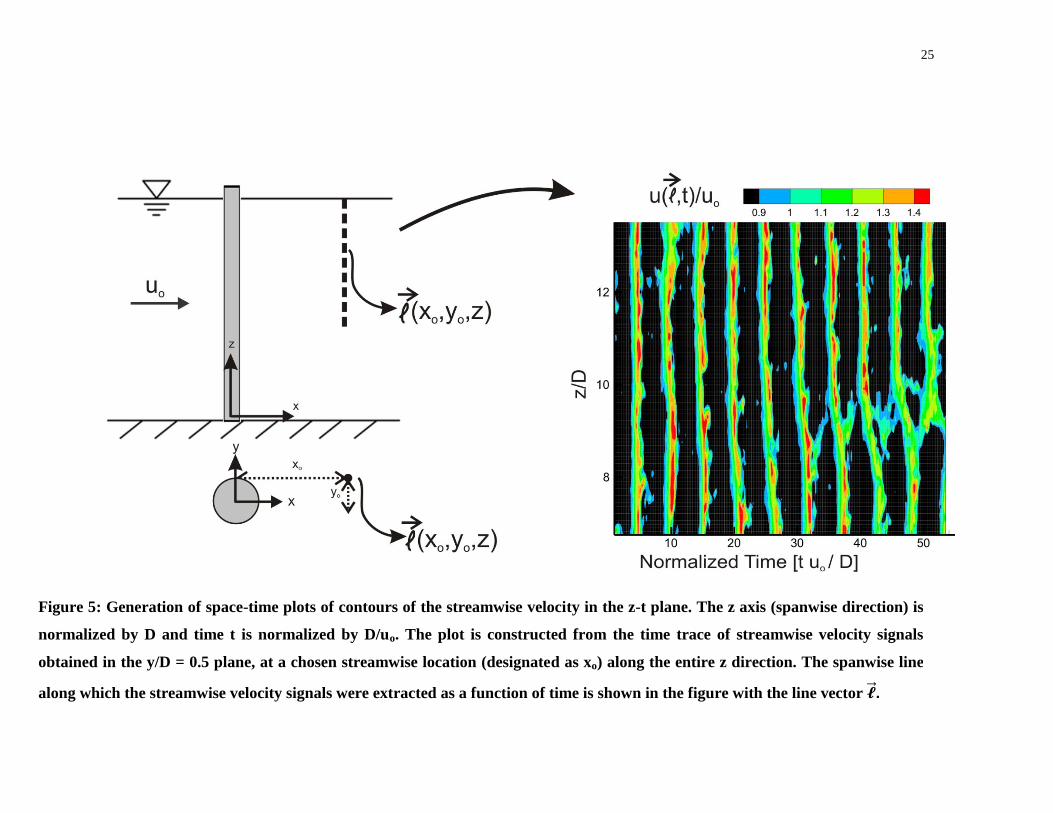
Figure 5: Generation of space-time plots of contours of the streamwise velocity in the z-t plane. The

z axis (spanwise direction) is normalized by D and time t is normalized by D/uo. The plot is

constructed from the time trace of streamwise velocity signals obtained in the y/D = 0.5 plane, at a

chosen streamwise location (designated as xo) along the entire z direction. The spanwise line along

which the streamwise velocity signals were extracted as a function of time is shown in the figure

with the line vector . .......................................................................................................................... 25

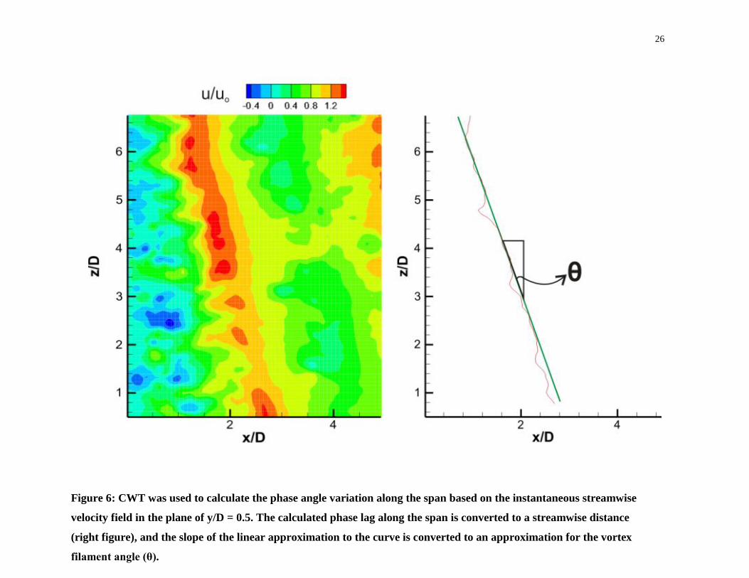
Figure 6: CWT was used to calculate the phase angle variation along the span based on the

instantaneous streamwise velocity field in the plane of y/D = 0.5. The calculated phase lag along the

span is converted to a streamwise distance (right figure), and the slope of the linear approximation to

the curve is converted to an approximation for the vortex filament angle (θ). ................................... 26

viii

Figure 7: Ensemble averaged results of the streamwise velocity yield a demarcation line between the

recirculation and positive velocity flow. Formation length as a function of spanwise location at

varying Re is shown for a cylinder bounded by the channel floor and the free-surface. As Re

increases free-surface effects are causing oblique shedding. .............................................................. 37

Figure 8: Formation length as a function of spanwise location at varying Re is shown for a cylinder

bounded by the channel floor and the channel top cover. As Re increases there is no major change to

shedding orientation. ........................................................................................................................... 37


bounded by sharp endplates at L/D of 2.5. As Re increases there is no major change to shedding

orientation. .......................................................................................................................................... 38


bounded by elliptical endplates at L/D of 2.5. As Re increases there is no major change to shedding

orientation. .......................................................................................................................................... 38

Figure 11: Free-surface effect causes a downward flow near the top, rear portion of the cylinder.

This leads to spanwise non-uniformities and introduces three-dimensionalities to the flow. The right

image shows the velocity vector map superimposed over the streamwise velocity contours. ........... 39

Figure 12: The velocity vector map is superimposed over the streamwise velocity contours for three

cases. A reduction in spanwise flow, and hence a decrease in three-dimensionalities is found if a top

cover or endplate is used. a) Cylinder is bounded on top by the channel cover. b) Cylinder is

bounded on top by a sharp leading edge geometry endplate. c) Cylinder is bounded on top by an

elliptical leading edge geometry endplate. .......................................................................................... 40

Figure 13: Space-time plots of the streamwise velocity and their corresponding vortex filament angle

plots for a cylinder bounded by the channel floor and the free-surface. Vortex splitting is seen in the

right most images of this figure. ......................................................................................................... 41

ix


plots for the top field of view of a cylinder bounded by the channel floor and channel cover. Minimal

variation in the vortex filament angles are found for this configuration. ........................................... 42


plots for the bottom field of view of a cylinder bounded by the channel floor and channel cover.

Slightly more variation is found than in the previous image, but it is still minimal compared to most

cases. ................................................................................................................................................... 43


plots for a cylinder bounded by a sharp leading edge endplate at L/D = 1 and the free-surface. ....... 44


plots for a cylinder bounded by a sharp leading edge endplate at L/D = 2.5 and the free-surface. .... 45


plots for a cylinder bounded by a sharp leading edge endplate at L/D = 5 and the free-surface. ....... 46


plots for a cylinder bounded by an elliptical leading edge endplate at L/D = 1.0 and the free-surface.

............................................................................................................................................................. 47



The fourth set of data for this configuration was corrupted. ............................................................... 48



............................................................................................................................................................. 49


plots for a cylinder bounded by a sharp leading edge endplate at L/D = 2.5 on the top and bottom. 50

x


plots for a cylinder bounded by a sharp leading edge endplate at L/D = 5 on the top and bottom. ... 51

Figure 24: Probability density function of the vortex filament angle for a cylinder bounded by a

sharp leading edge endplate and the free-surface for various L/D values. ......................................... 52

Figure 25: Probability density function of the vortex filament angle for a cylinder bounded by an

elliptical leading edge endplate and the free-surface for various L/D values. .................................... 53

Figure 26: Probability density function of the vortex filament angle for a cylinder bounded by the

channel floor and the free-surface. ...................................................................................................... 54

Figure 27: Probability density function of the vortex filament angle for a cylinder bounded by a

sharp leading edge endplate on top and bottom for two L/D values. ................................................. 55

Figure 28: Probability density function of the vortex filament angle for a cylinder bounded by an

elliptical leading edge endplate on top and bottom for two L/D values. ............................................ 56

Figure 29: Vortex Splitting was observed in the space-time plots for all boundary conditions

analyzed. ............................................................................................................................................. 57

Figure 30: Comparing the stream-wise velocity signals for a point in the flow where a split has

occurred and one that has undergone normal shedding. The vortex split causes attenuation of the

velocity signal. .................................................................................................................................... 58

Figure 31: The stream-wise velocity signal in a window where there is a reduction in the spectral

density of the Karman Strouhal number shows attenuation similar to that found when a vortex split is

present. ................................................................................................................................................ 59

Figure 32: Bar Graphs displaying the number of occurrences of each range of Vortex Filament

Angles prior to a vortex split for cases in which the end configuration does not promote parallel

shedding. Note that the most likely shedding orientation prior to a vorte .......................................... 64

xi

Figure 33: Bar Graphs displaying the number of occurrences of each range of Vortex Filament

Angles prior to a vortex split for cases in which the end configuration promotes parallel shedding.

Note that the vortex filament angle takes on nearly all values before a vortex split .......................... 65

1

Introduction 1

1.1 Motivation and Background

Due to their practical importance, flow dynamics related to vortex shedding behind a bluff body has

been the subject of intense research across a variety of engineering fields. The main model used to

represent bluff bodies is traditionally a cylinder. Early researchers characterized the flow around

cylinders for a range of upstream flow conditions. The alternate shedding of vortices on the cylinder

was shown to lead to large pressure imbalances and subsequent vortex-induced vibrations (VIVs) on

the body. VIVs have negative effects on the structure, and can lead to a loss of structural integrity,

threatening the fatigue life of the system. Therefore being able to understand and control the near-

wake of a cylinder, and hence suppress the VIVs, have been the goal of many researchers.

The majority of the bluff bodies in practical applications, such as riser tubes, cables, towers, bridges

and chimney stacks, have a length much greater than their diameter, and hence can be rendered as

infinitely long. For such bodies, the wakes and the resulting VIVs are not influenced by the end

boundaries. However, in a finite experimental setup, where the effects from the end boundaries of

the body cannot be underestimated, a method to minimize the end effects is deemed necessary for

the experimental work to ensure that any concepts developed would not be limited to the specific

laboratory arrangement, but would have universal effectiveness. Consequently the primary goal of

this thesis is to examine how different end conditions applied on a cylinder affect its near wake, and

to generate a method to properly model an infinite cylinder in a laboratory experiment.

The first chapter of the thesis will provide an introduction to the topic and a summary of the previous

work related to this field of study. Chapter two will discuss the experimental setup and the different

analysis techniques employed. Chapter three includes the results and findings on test models with

different end conditions. Finally, chapter four concludes the paper and presents recommendations for

future work on the subject.

2

1.2 Literature Review

1.2.1 Flow Past an Infinite Cylinder

The mechanism of vortex formation was qualitatively explained first by Gerrard [1]. He suggested

that as a vortex forms and increases its strength from one side of the cylinder, it draws the shear

layer from the opposite side, across the wake centerline. Eventually, this opposite shear layer cuts of

the supply of vorticity to the growing vortex. This process repeats alternately between the two shear

layers, leading to the alternate shedding of Karman vortices.

A few key definitions are needed before progressing in the literature review: The first definition is

the formation length, FL, which is the length of the mean recirculation region in the near-wake of a

cylinder. This is a bubble shaped region, which is symmetric with respect to near-wake centerline.

The formation length can be identified as the point downstream of the bluff body where the velocity

fluctuations make a maximum. The second key definition is the base suction coefficient, -Cpb, which

is defined as the negative value of the pressure coefficient at the back of the cylinder.

The characteristics of the flow past a cylinder are shown to greatly depend on the Reynolds number

of the flow. Following is a breakdown of the different regimes (based on the Reynolds number) [2].

For small Reynolds numbers (Re < ~49), the flow is said to be in the laminar steady regime. In this

regime, the flow is time independent, and the mean recirculation zone is two symmetrical fixed

eddies. As the Reynolds number increases (Re = ~49 to ~190), the flow becomes unsteady and the

flow enters the laminar vortex shedding regime. Due to instabilities in the near-wake, a von Karman

vortex street is developed in this regime. With increasing Reynolds number (Re ~190 to 260), the

flow enters the wake transition regime. Here, three-dimensional characteristics are introduced to the

wake. Also, two discontinuities in the wake formation are found. These discontinuities are due to

two different instabilities, called as mode A and mode B, which appear to have hysteretic

characteristic. Up to this point, as the Reynolds number increases, the base suction coefficient, and

the Strouhal frequency increases, while the formation length decreases. At a Reynolds number of

approximately 260, there is a peak in Reynolds stresses in the near wake and the trends mentioned

above all reverse with an increase in Reynolds number. As Reynolds number increases from 260

until about 1,000, three-dimensional fine scale streamwise vortex structures become increasingly

3

disordered in the near wake while the boundary layer stays laminar. The next regime, known as the

sub-critical regime (or shear-layer transition regime), encompasses the Reynolds number values of

Re = 1,000 to 200,000. The experiments in this thesis fall within this regime. The main

characteristics of this regime are that, with increasing Reynolds number, fluctuation increases, base

suction increases, Strouhal number decreases, and the formation length decreases. These trends are

caused by the increased unsteadiness of the shear layers, separating from the sides of the body. In

addition, in this regime, small-scale vortical structures in the separating shear layers due to the

Kelvin-Helmholtz instability (also known as shear-layer instability) develop and additionally

increase the base suction and the Reynolds stresses. As the Reynolds number increases in this sub-

critical regime, the turbulence transition point (i.e., the onset location of the shear-layer instability)

moves upstream toward the surface of the body. So the turbulent transition occurs somewhere within

the separating shear layers. In a narrow Reynolds number range past 200,000, the turbulent transition

point moves upstream such that it enters the boundary layer on the cylinder surface. The boundary

layer becomes turbulent at the separation point, but this occurs at only one side of the cylinder, while

the boundary-layer separation remains laminar on the other side. As a result, a separation-

reattachment bubble forms on the side where turbulent separation occurs, causing an asymmetric lift

vector that can have quite a large magnitude. Turbulent boundary-layer separation switches in this

regime from one side of the cylinder to the other, causing a change in the lift vector direction

occasionally. The flow with these characteristics is said to be in the critical (or lower transition) flow

regime. Both the base suction and the drag decrease drastically in this regime due to a phenomenon

known as drag crisis. Past the critical regime, the flow enters the symmetric reattachment regime,

also known as the supercritical regime. In this regime the flow is characterized by turbulent

boundary-layer separation on both sides of the cylinder and the flow is symmetric with two

symmetric separation-reattachment bubbles. In this regime, the transition point in the boundary layer

is somewhere between the stagnation point and the separation point, that is, the boundary layer is

partly laminar and partly turbulent. Finally, at higher Reynolds numbers, the entire boundary layer

on the surface of the cylinder becomes turbulent. This is known as the boundary-layer transition

regime, or the post-critical regime.

4

1.2.2 End Effects on the Spanwise Uniformity of the Cylinder Near Wake

Eisenlohr and Eckelmann [3] showed that in the laminar vortex shedding regime, the oblique angle

of vortex shedding can be as high as 30o

. As the oblique angle further increased, the vortex would

split, in a phenomenon known as vortex splitting. While attempting to cause vortex splitting by using

larger diameter cylinders at the end of the original cylinder, they discovered that the flow had

become more parallel. Eisenlohr and Eckelmann postulated that the original oblique shedding is due

to the end of the vortex axes being curved by the horseshoe vortex (HSV) formed by the boundary

layer of the wall. This curvature causes strain on the entire vortex axes and leads to an oblique angle

being formed. Upon placing larger diameter cylinders at the ends, the vortex splits before it can be

curved by the horseshoe vortex, preventing any strain on the initial axes.

Eisenlohr and Ecklemann were among the first to observe vortex dislocations. They showed that the

Strouhal number (St) is not always constant along the span of a cylinder. This can occur for a

multitude of reasons, but is most likely due to non-uniformities in the oncoming flow. If there is a

large difference in St along the span, oblique shedding is formed. This may cause a phenomenon

known as vortex dislocation to occur if the shedding at the interface of two cells of different

frequency is out of phase. Eisenlohr and Ecklemann placed cylinders of slightly larger diameters on

either end of the test cylinder to ensure that there would be a jump in the frequency of shedding.

They observed vortex dislocations occurring at the beat frequency between the cylinders of different

diameters. This led them to believe that as the phase angle between the two shedding cycles grows in

magnitude a dislocation of the vortex filament is found, and due to the conservation of circulation

the filament must either be short-circuited with its counterpart or divide up its circulation among

neighboring filaments of the same vorticity. The latter option is referred to as vortex splitting. At

lower Re, Re<300, vortex dislocations are found only when oblique shedding is present and there are

cells of different frequency along the span.

Also within the laminar vortex shedding regime, Williamson [4] was able to manipulate the end

conditions of the flow, by introducing slanted endplates, so as to create a quasi-two dimensional

flow. In the absence of endplates, the end cells of the cylinder have a higher base pressure than the

midspan, which enlarges the vortex formation region, in turn reducing the shedding frequency.

Parallel shedding can be induced by decreasing the base pressure at the end cells; increasing the

5

shedding frequency near the ends to match that of the midspan. This allowed for the development of

a continuous Strouhal-Reynolds curve, which was shown to be reproducible in other experimental

facilities.

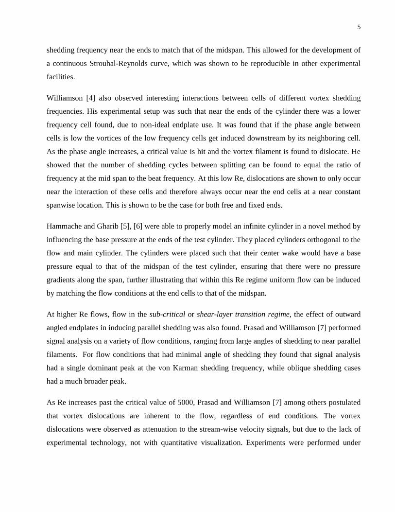
Williamson [4] also observed interesting interactions between cells of different vortex shedding

frequencies. His experimental setup was such that near the ends of the cylinder there was a lower

frequency cell found, due to non-ideal endplate use. It was found that if the phase angle between

cells is low the vortices of the low frequency cells get induced downstream by its neighboring cell.

As the phase angle increases, a critical value is hit and the vortex filament is found to dislocate. He

showed that the number of shedding cycles between splitting can be found to equal the ratio of

frequency at the mid span to the beat frequency. At this low Re, dislocations are shown to only occur

near the interaction of these cells and therefore always occur near the end cells at a near constant

spanwise location. This is shown to be the case for both free and fixed ends.

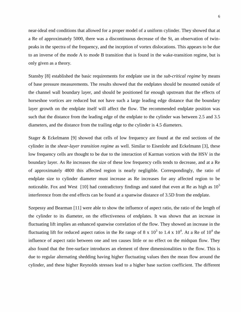
Hammache and Gharib [5], [6] were able to properly model an infinite cylinder in a novel method by

influencing the base pressure at the ends of the test cylinder. They placed cylinders orthogonal to the

flow and main cylinder. The cylinders were placed such that their center wake would have a base

pressure equal to that of the midspan of the test cylinder, ensuring that there were no pressure

gradients along the span, further illustrating that within this Re regime uniform flow can be induced

by matching the flow conditions at the end cells to that of the midspan.

At higher Re flows, flow in the sub-critical or shear-layer transition regime, the effect of outward

angled endplates in inducing parallel shedding was also found. Prasad and Williamson [7] performed

signal analysis on a variety of flow conditions, ranging from large angles of shedding to near parallel

filaments. For flow conditions that had minimal angle of shedding they found that signal analysis

had a single dominant peak at the von Karman shedding frequency, while oblique shedding cases

had a much broader peak.

As Re increases past the critical value of 5000, Prasad and Williamson [7] among others postulated

that vortex dislocations are inherent to the flow, regardless of end conditions. The vortex

dislocations were observed as attenuation to the stream-wise velocity signals, but due to the lack of

experimental technology, not with quantitative visualization. Experiments were performed under

6

near-ideal end conditions that allowed for a proper model of a uniform cylinder. They showed that at

a Re of approximately 5000, there was a discontinuous decrease of the St, an observation of twin-

peaks in the spectra of the frequency, and the inception of vortex dislocations. This appears to be due

to an inverse of the mode A to mode B transition that is found in the wake-transition regime, but is

only given as a theory.

Stansby [8] established the basic requirements for endplate use in the sub-critical regime by means

of base pressure measurements. The results showed that the endplates should be mounted outside of

the channel wall boundary layer, and should be positioned far enough upstream that the effects of

horseshoe vortices are reduced but not have such a large leading edge distance that the boundary

layer growth on the endplate itself will affect the flow. The recommended endplate position was

such that the distance from the leading edge of the endplate to the cylinder was between 2.5 and 3.5

diameters, and the distance from the trailing edge to the cylinder is 4.5 diameters.

Stager & Eckelmann [9] showed that cells of low frequency are found at the end sections of the

cylinder in the shear-layer transition regime as well. Similar to Eisenlohr and Eckelmann [3], these

low frequency cells are thought to be due to the interaction of Karman vortices with the HSV in the

boundary layer. As Re increases the size of these low frequency cells tends to decrease, and at a Re

of approximately 4800 this affected region is nearly negligible. Correspondingly, the ratio of

endplate size to cylinder diameter must increase as Re increases for any affected region to be

noticeable. Fox and West [10] had contradictory findings and stated that even at Re as high as 105

interference from the end effects can be found at a spanwise distance of 3.5D from the endplate.

Szepessy and Bearman [11] were able to show the influence of aspect ratio, the ratio of the length of

the cylinder to its diameter, on the effectiveness of endplates. It was shown that an increase in

fluctuating lift implies an enhanced spanwise correlation of the flow. They showed an increase in the

fluctuating lift for reduced aspect ratios in the Re range of 8 x 103 to 1.4 x 10

4. At a Re of 10

4 the

influence of aspect ratio between one and ten causes little or no effect on the midspan flow. They

also found that the free-surface introduces an element of three dimensionalities to the flow. This is

due to regular alternating shedding having higher fluctuating values then the mean flow around the

cylinder, and these higher Reynolds stresses lead to a higher base suction coefficient. The different

7

values of base suction coefficient lead to a span wise flow, and an increase in oblique shedding near

the free-surface

Szepessy [12] showed that any phase drift in the vortex shedding will cause instantaneous pressure

gradients along the span, disrupting the vortex shedding regularity. To generate ideal two-

dimensionality in shedding in the shear-layer transition regime a minimum leading edge distance

between the cylinder and endplate must be 1.5D while the trailing edge distance must be at least

3.5D. For different Re regimes, the trailing edge distance must always be longer then the vortex

formation region to ensure a uniform base pressure along the cylinder. Szepessy further shows that

for proper endplate use, there is a minimal pressure gradient two diameters downstream of the

cylinder in the spanwise direction.

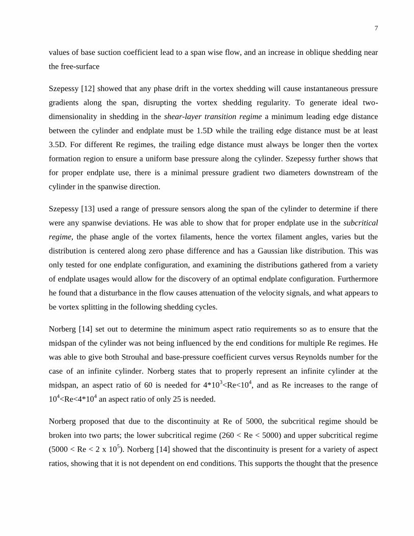
Szepessy [13] used a range of pressure sensors along the span of the cylinder to determine if there

were any spanwise deviations. He was able to show that for proper endplate use in the subcritical

regime, the phase angle of the vortex filaments, hence the vortex filament angles, varies but the

distribution is centered along zero phase difference and has a Gaussian like distribution. This was

only tested for one endplate configuration, and examining the distributions gathered from a variety

of endplate usages would allow for the discovery of an optimal endplate configuration. Furthermore

he found that a disturbance in the flow causes attenuation of the velocity signals, and what appears to

be vortex splitting in the following shedding cycles.

Norberg [14] set out to determine the minimum aspect ratio requirements so as to ensure that the

midspan of the cylinder was not being influenced by the end conditions for multiple Re regimes. He

was able to give both Strouhal and base-pressure coefficient curves versus Reynolds number for the

case of an infinite cylinder. Norberg states that to properly represent an infinite cylinder at the

midspan, an aspect ratio of 60 is needed for 4*103<Re<10

4, and as Re increases to the range of

104<Re<4*10

4 an aspect ratio of only 25 is needed.

Norberg proposed that due to the discontinuity at Re of 5000, the subcritical regime should be

broken into two parts; the lower subcritical regime (260 < Re < 5000) and upper subcritical regime

(5000 < Re < 2 x 105). Norberg [14] showed that the discontinuity is present for a variety of aspect

ratios, showing that it is not dependent on end conditions. This supports the thought that the presence

8

of vortex dislocations is a fundamental feature of the flow in this Re regime. Along with Prasad and

Williamson[7], both Norberg and Szepessy [13] showed the presence of dislocations in this Re range

for near uniform shedding.

This thesis will further examine the unsteady nature of vortex shedding in the sub-critical regime

proposed by Szepessy [13], by means of visualization of the near-wake. Furthermore multiple end

configurations will be analyzed as opposed to just the single case studied by Szepessy, allowing for

insight into how different end conditions impact the flow past a cylinder. Finally the ability to

quantitatively visualize the flow in the near-wake will allow for the confirmation of the presence of

vortex splitting in the sub-critical regime. This will help confirm the findings of previous authors

[7], [13], [14], as well as further the study into the formation and characteristics of the phenomenon.

9

Experimental Setup and Analysis Techniques 2

2.1 Experimental Setup

2.1.1 Water Channel

Data acquisition was undertaken in the experimental fluids research laboratory at the Institute for

Aerospace Studies at the University of Toronto. The experimental models were placed in a state-of

the-art recirculating water channel. The main test section extends 5 m in in the horizontal direction,

and has a cross-section of 610 mm by 686 mm. The channel has a flow speed controller, a returning

plenum, a settling chamber composed of a honeycomb and a set of screens, and a 6:1 contraction

section. This channel can provide continuous flow in the horizontal direction either in free-surface

mode or through the placement of top covers in fully-covered mode as a tunnel. In free-surface

mode, free-surface turbulence intensity was less than 0.5% and the flow uniformity was better than

0.3%. When the top covers of the channel were in place, it achieved a turbulence intensity of less

than 0.4% and a flow uniformity of better than 0.1%. The range of Reynolds numbers examined was

4x103

- 36x103 based on the cylinder diameter. The water temperature was shown to vary from 18 °C

to 24 °C, depending on the outside temperature. To avoid fluctuations in the value of the Reynolds

number due to such temperature changes, the temperature of the water was measured frequently over

the course of experiments and the free-stream velocity, uo, was adjusted accordingly.

2.1.2 Test models

The cylinders were mounted in the vertical orientation inside the water channel, equidistant from

both side walls. Each cylinder was fixed to a traverse outside of the water channel, which ensured

that there was no cylinder vibration. The length of the cylinder in which shed vortices will be

investigated is denoted as S and D represents the diameter. The cylinders used in the experiments

have a diameter of D = 50.8 mm. This gave a maximum aspect ratio S/D of 13.5 for the water

channel being used, which is below the minimum aspect ratio to be able to neglect end effects [14].

A cylinder of diameter of 50.8 mm is selected to ensure that the flow dynamics of the wake can

properly be visualized with the vector resolution available from PIV.

10

A right handed Cartesian coordinate system will be used for all the experiments presented in the

thesis. The origin of the axis will be at the center of the bottom of a cylinder with no endplate, and

the x, y and z axis represent the stream-wise, transverse and spanwise directions respectively.

To explore the effect of various end conditions on the wake three-dimensionality, different end

boundaries were designed for cylinder models. For those involving an endplate boundary,

consideration was given to two different leading-edge shapes: One involved a sharp leading edge

with a bevel angle of 23.6° and the other had a super-elliptical nose shape with an axes ratio of 6.

The latter shape adopted with an axes ratio of 6 and above was reported to result in laminar

boundary layer along the plate by Narasimha and Prasad [15]. All end plates had a thickness of 12.7

mm, a total length of 7.5D (following the recommendations of Stansby [6]) and a width equal to the

entire width of the channel 12D. The different end configurations considered in the present

investigation are sketched in figure 1. They are as detailed below:

a) A cylinder bounded by the channel floor at the bottom end and the free-surface at the top.

(S/D = 13.5)

b) A cylinder bounded by the channel floor at the bottom and a top-cover at the top. This is also

referred to, in the text, as the wall-wall boundary condition. The top-cover was designed to

have an opening for the cylinder to pass through. (S/D = 13.5)

c) A cylinder bounded by the endplate with a sharp leading edge at the bottom and the free-

surface at the top. As indicated above, the bevel angle of the sharp leading edge was 23.6o.

(S/D = 12.3)

d) A cylinder bounded by the endplate with an elliptical leading edge at the bottom and the free-

surface at the top. As indicated, the axes ratio of the elliptical nose shape was 6. This

elliptical leading edge was found to prevent flow separation at the leading edge of the

endplate by Blackmore [16] (S/D = 12.3)

e) A cylinder bounded by endplates at both ends. This scenario involved the use of two

endplates with the sharp leading edge, bevel angle of which was 23.6o. (S/D = 10.8)

f) A cylinder bounded by endplates at both ends. Both endplates used in this case had the

elliptical leading edge. (S/D = 10.8)

11

The cylinder was mounted approximately 21D downstream from the entrance of the test section in

each experiment. At this location, the boundary layer forming along the channel floor, with no

cylinder present, was determined to be 0.25D at a Reynolds number value of 104. For those

configurations where an end plate was used at the bottom end, the endplate was lifted such that the

bottom end of the cylinder was 1.25D way from the channel floor to ensure that there would be no

direct influence from the channel floor’s boundary layer. As for the configurations in which a top

plate was used, the end plate was placed such that the end of the cylinder had a distance of 1.5D

from the free-surface, which corresponds to a location of 0.87 z/S. This is a sufficient distance from

the free-surface as Farivar [17] found that the maximum in fluctuating pressure due to free-surface

effects occur closer to the free-surface, at a z/S value of 0.95.

Let L designate the distance between the leading edge of an endplate and the center of the cylinder.

For the configurations where endplates were employed, multiple L/D values were tested to

determine the significance of the cylinder location on the end plate. For situations in which the

cylinder was bounded by one endplate at the bottom and the free-surface at the top, L/D values range

from 1 to 6. For the case of the cylinder being bounded by endplates on both the top and the bottom,

the range of L/D values examined was 2 to 6 due to restrictions on the ability to properly fix the

cylinder between the two endplates.

2.1.3 Particle Image Velocimetry

Quantitative visualization of the flow in the wake region will be obtained via a cinema technique of

Particle Image Velocimetry (PIV). There are four main components of a PIV setup: a CCD camera, a

double-pulsed Nd:YAG laser system, a data acquisition computer equipped with the appropriate

frame grabber, and a synchronizer. Tracer particles that are made up of small glass beads with

neutral buoyancy and diameter of about 14 microns are mixed into the water channel. A set of lenses

(cylindrical and spherical) are used to transform the laser beam to a laser sheet to illuminate the

tracer particles as they pass through the visualization plane of interest. The thickness of the laser

sheet was kept constant for all experimental configurations. The camera is setup perpendicular to the

laser sheet. Both the digital camera and the laser system are connected to the synchronizer and the

computer. The camera provided a magnification factor of 4.7 pixels per millimeter and a spatial grid

resolution of 0.67D was used for all experiments. Particle images are captured in pairs, and the

12

cross-correlation of the images in each pair through software named INSIGHT provides the velocity

vector field. A recursive Nyquist grid algorithm compared the two images that were captured at a

specified time difference to develop a flow field in pixels per second for each pair. The Δt between

pairs was chosen carefully to optimize the output of the algorithm by ensuring there was the

appropriate average displacement of particles for each set of frames. After processing the images

with INSIGHT, a second program named CleanVec was used to remove any spurious vectors

produced by the algorithm. Finally, a post-processor was used to convert the units of the velocity

vectors to mm/s as well as positions to mm as opposed to pixels.

As outlined by Raffel et. al. [18] to compensate for the out-of-plane loss of particle pairs the laser

light sheet was arranged to have a thickness of 1 mm. The PIV system employed can provide only a

coarse frequency resolution as opposed to the constant temperature anemometers, which are

described in the following section. This bottleneck of the PIV system is due to both the limitation of

the capturing time over a sequence due to the available RAM memory of the computer, and the low

sampling rate. That is, the PIV system used has a maximum sampling frequency of 14.5 Hz, and is

limited to acquiring 200 sets of images per experiment. Hence, the frequency resolution of the data

acquired by this system is 0.07 Hz. Despite the disadvantage of coarse frequency resolution, PIV

measurements provide a non-intrusive method for quantitative visualization of the global flow

features. With the knowledge of the average shedding frequency at different Re, given by [14], an

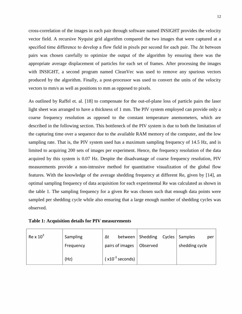
optimal sampling frequency of data acquisition for each experimental Re was calculated as shown in

the table 1. The sampling frequency for a given Re was chosen such that enough data points were

sampled per shedding cycle while also ensuring that a large enough number of shedding cycles was

observed.

Table 1: Acquisition details for PIV measurements

Re x 103

Sampling

Frequency

(Hz)

Δt between

pairs of images

( x10-3 seconds)

Shedding Cycles

Observed

Samples per

shedding cycle

13

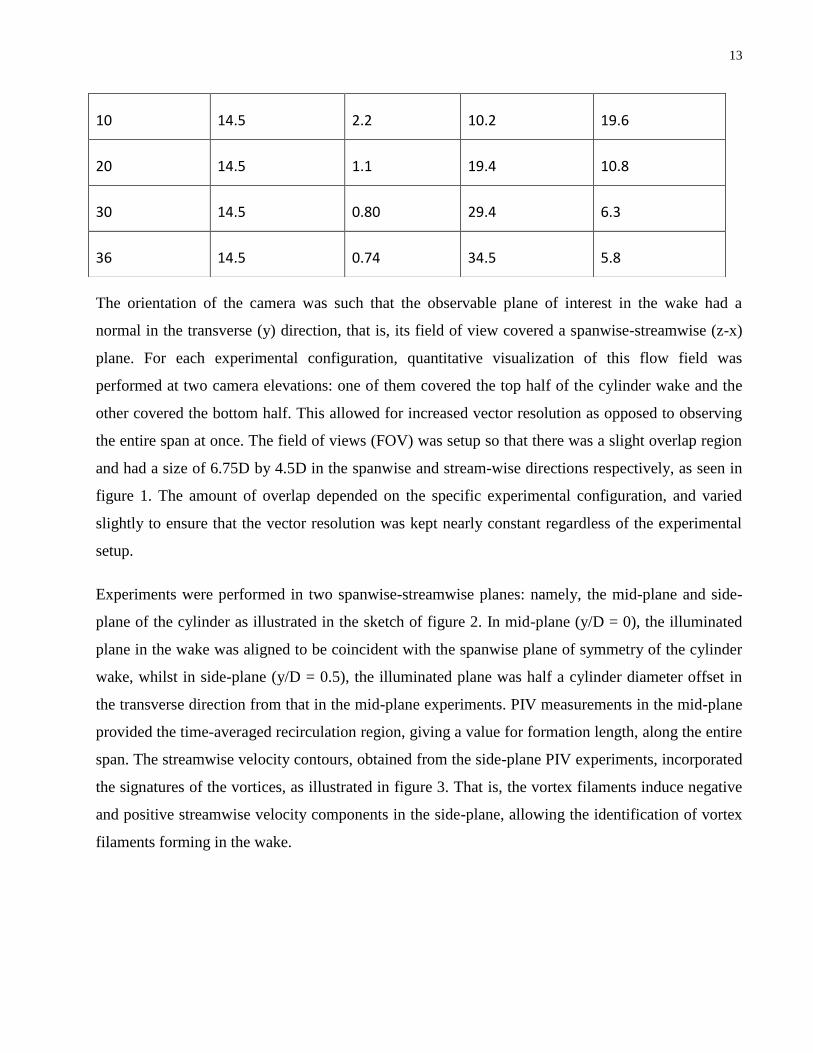
The orientation of the camera was such that the observable plane of interest in the wake had a

normal in the transverse (y) direction, that is, its field of view covered a spanwise-streamwise (z-x)

plane. For each experimental configuration, quantitative visualization of this flow field was

performed at two camera elevations: one of them covered the top half of the cylinder wake and the

other covered the bottom half. This allowed for increased vector resolution as opposed to observing

the entire span at once. The field of views (FOV) was setup so that there was a slight overlap region

and had a size of 6.75D by 4.5D in the spanwise and stream-wise directions respectively, as seen in

figure 1. The amount of overlap depended on the specific experimental configuration, and varied

slightly to ensure that the vector resolution was kept nearly constant regardless of the experimental

setup.

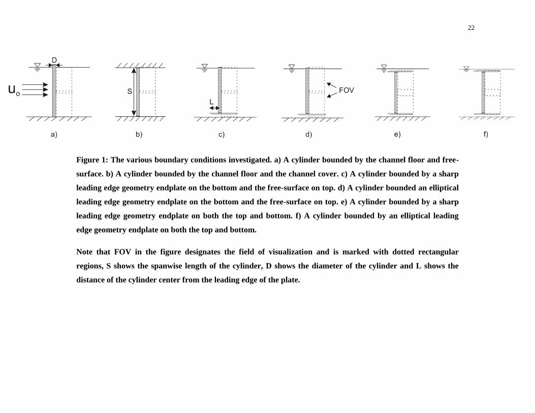
Experiments were performed in two spanwise-streamwise planes: namely, the mid-plane and side-

plane of the cylinder as illustrated in the sketch of figure 2. In mid-plane (y/D = 0), the illuminated

plane in the wake was aligned to be coincident with the spanwise plane of symmetry of the cylinder

wake, whilst in side-plane (y/D = 0.5), the illuminated plane was half a cylinder diameter offset in

the transverse direction from that in the mid-plane experiments. PIV measurements in the mid-plane

provided the time-averaged recirculation region, giving a value for formation length, along the entire

span. The streamwise velocity contours, obtained from the side-plane PIV experiments, incorporated

the signatures of the vortices, as illustrated in figure 3. That is, the vortex filaments induce negative

and positive streamwise velocity components in the side-plane, allowing the identification of vortex

filaments forming in the wake.

10 14.5 2.2 10.2 19.6

20 14.5 1.1 19.4 10.8

30 14.5 0.80 29.4 6.3

36 14.5 0.74 34.5 5.8

14

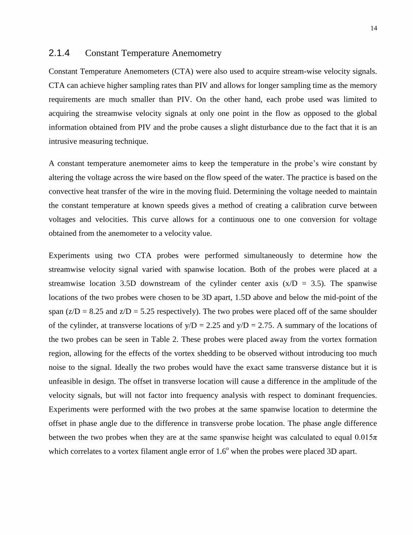
2.1.4 Constant Temperature Anemometry

Constant Temperature Anemometers (CTA) were also used to acquire stream-wise velocity signals.

CTA can achieve higher sampling rates than PIV and allows for longer sampling time as the memory

requirements are much smaller than PIV. On the other hand, each probe used was limited to

acquiring the streamwise velocity signals at only one point in the flow as opposed to the global

information obtained from PIV and the probe causes a slight disturbance due to the fact that it is an

intrusive measuring technique.

A constant temperature anemometer aims to keep the temperature in the probe’s wire constant by

altering the voltage across the wire based on the flow speed of the water. The practice is based on the

convective heat transfer of the wire in the moving fluid. Determining the voltage needed to maintain

the constant temperature at known speeds gives a method of creating a calibration curve between

voltages and velocities. This curve allows for a continuous one to one conversion for voltage

obtained from the anemometer to a velocity value.

Experiments using two CTA probes were performed simultaneously to determine how the

streamwise velocity signal varied with spanwise location. Both of the probes were placed at a

streamwise location 3.5D downstream of the cylinder center axis (x/D = 3.5). The spanwise

locations of the two probes were chosen to be 3D apart, 1.5D above and below the mid-point of the

span (z/D = 8.25 and z/D = 5.25 respectively). The two probes were placed off of the same shoulder

of the cylinder, at transverse locations of y/D = 2.25 and y/D = 2.75. A summary of the locations of

the two probes can be seen in Table 2. These probes were placed away from the vortex formation

region, allowing for the effects of the vortex shedding to be observed without introducing too much

noise to the signal. Ideally the two probes would have the exact same transverse distance but it is

unfeasible in design. The offset in transverse location will cause a difference in the amplitude of the

velocity signals, but will not factor into frequency analysis with respect to dominant frequencies.

Experiments were performed with the two probes at the same spanwise location to determine the

offset in phase angle due to the difference in transverse probe location. The phase angle difference

between the two probes when they are at the same spanwise height was calculated to equal 0.015π

which correlates to a vortex filament angle error of 1.6o when the probes were placed 3D apart.

15

The CTA systems used were from Dantec Dynamics. The probes were connected to a MiniCTA

system, which in turn was connected to the computer via a shielded connector block from national

instruments (NI BNC 2110). This allowed for acquisition of stream-wise velocity signals from

multiple probes. The characteristics of each probe are given in Table 2. The probes were placed in

probe holders supplied by Dantec Dynamics (part 55H22) that had a 90° bend to allow for

acquisition of streamwise velocity signals while being mounted to the same traverse that the cylinder

is mounted to. CTA data was not possible with the top channel covers in place because there was no

opening to mount the probe holders. Likewise, for end boundary configurations where a top end-

plate had a small leading-edge distance (L/D < 3), CTA measurements were not possible due to the

long trailing distance of the endplate preventing the probe from reaching the desired downstream

location.

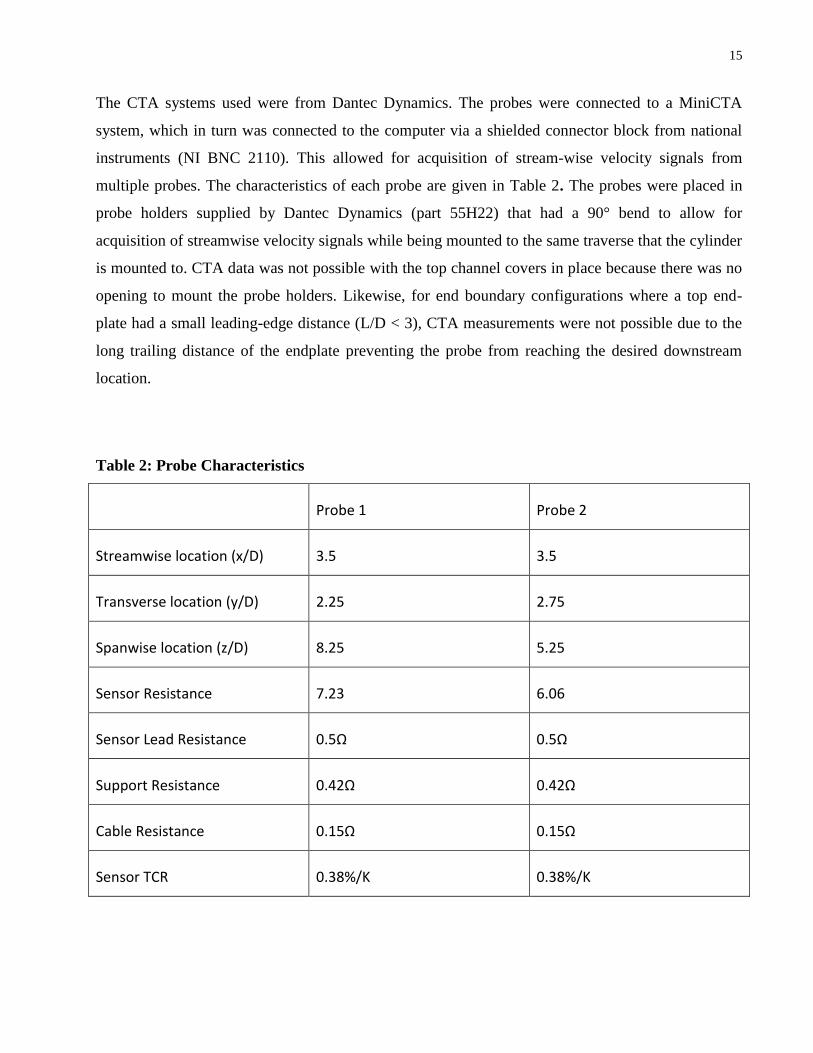
Table 2: Probe Characteristics

Probe 1 Probe 2

Streamwise location (x/D) 3.5 3.5

Transverse location (y/D) 2.25 2.75

Spanwise location (z/D) 8.25 5.25

Sensor Resistance 7.23 6.06

Sensor Lead Resistance 0.5Ω 0.5Ω

Support Resistance 0.42Ω 0.42Ω

Cable Resistance 0.15Ω 0.15Ω

Sensor TCR 0.38%/K 0.38%/K

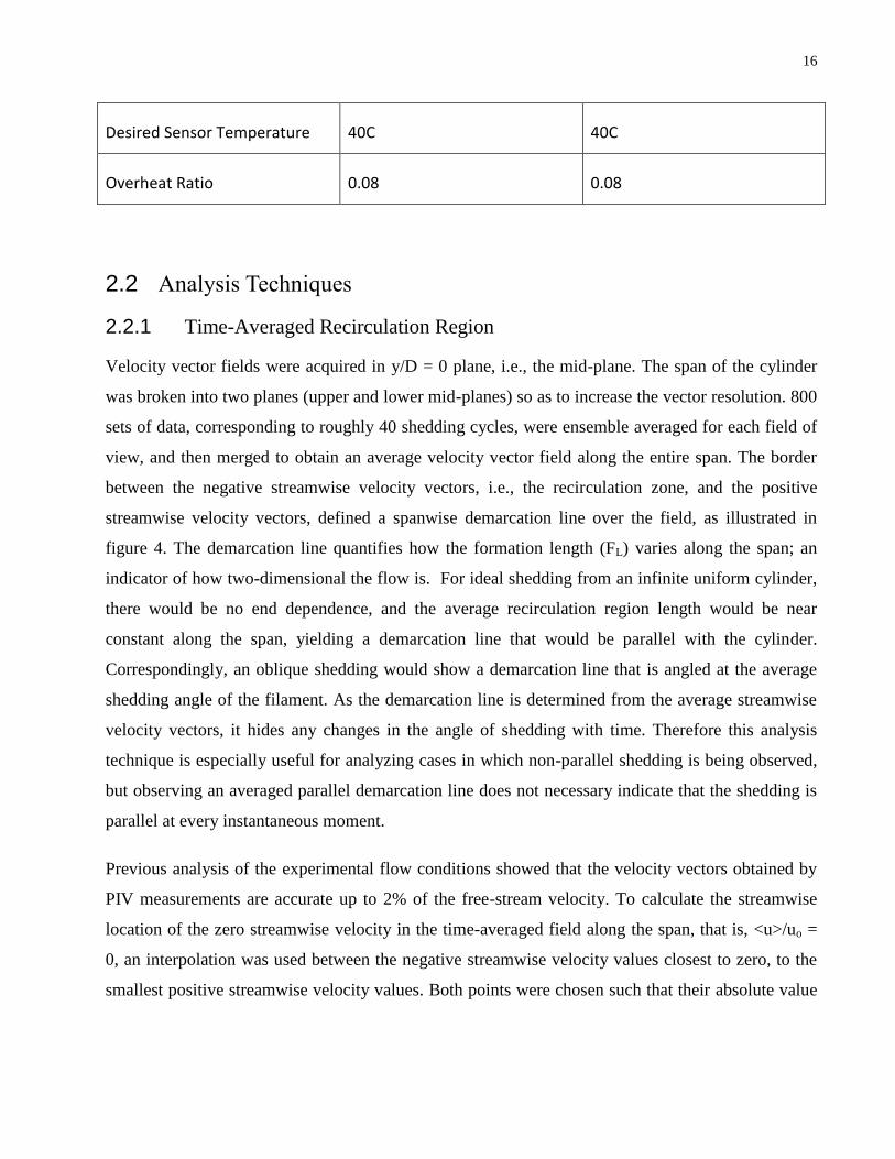
16

Desired Sensor Temperature 40C 40C

Overheat Ratio 0.08 0.08

2.2 Analysis Techniques

2.2.1 Time-Averaged Recirculation Region

Velocity vector fields were acquired in y/D = 0 plane, i.e., the mid-plane. The span of the cylinder

was broken into two planes (upper and lower mid-planes) so as to increase the vector resolution. 800

sets of data, corresponding to roughly 40 shedding cycles, were ensemble averaged for each field of

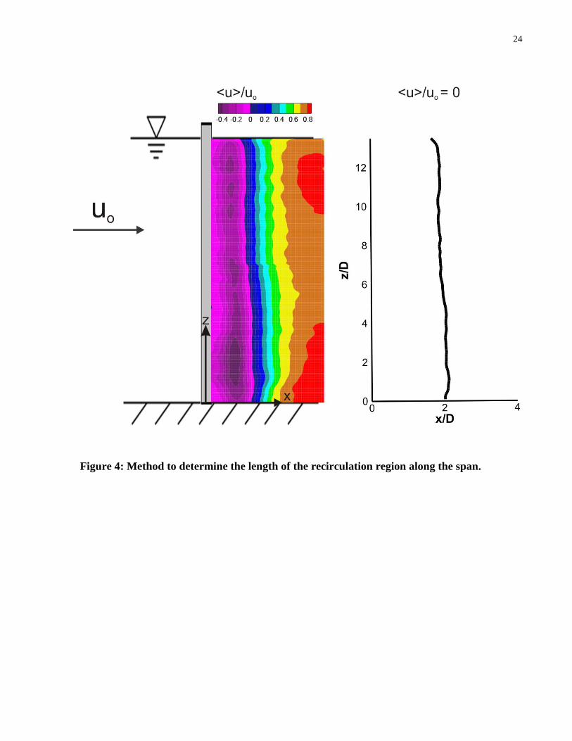
view, and then merged to obtain an average velocity vector field along the entire span. The border

between the negative streamwise velocity vectors, i.e., the recirculation zone, and the positive

streamwise velocity vectors, defined a spanwise demarcation line over the field, as illustrated in

figure 4. The demarcation line quantifies how the formation length (FL) varies along the span; an

indicator of how two-dimensional the flow is. For ideal shedding from an infinite uniform cylinder,

there would be no end dependence, and the average recirculation region length would be near

constant along the span, yielding a demarcation line that would be parallel with the cylinder.

Correspondingly, an oblique shedding would show a demarcation line that is angled at the average

shedding angle of the filament. As the demarcation line is determined from the average streamwise

velocity vectors, it hides any changes in the angle of shedding with time. Therefore this analysis

technique is especially useful for analyzing cases in which non-parallel shedding is being observed,

but observing an averaged parallel demarcation line does not necessary indicate that the shedding is

parallel at every instantaneous moment.

Previous analysis of the experimental flow conditions showed that the velocity vectors obtained by

PIV measurements are accurate up to 2% of the free-stream velocity. To calculate the streamwise

location of the zero streamwise velocity in the time-averaged field along the span, that is, <u>/uo =

0, an interpolation was used between the negative streamwise velocity values closest to zero, to the

smallest positive streamwise velocity values. Both points were chosen such that their absolute value

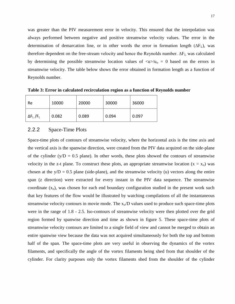
17

was greater than the PIV measurement error in velocity. This ensured that the interpolation was

always performed between negative and positive streamwise velocity values. The error in the

determination of demarcation line, or in other words the error in formation length (∆FL), was

therefore dependent on the free-stream velocity and hence the Reynolds number. ∆FL was calculated

by determining the possible streamwise location values of <u>/uo = 0 based on the errors in

streamwise velocity. The table below shows the error obtained in formation length as a function of

Reynolds number.

Table 3: Error in calculated recirculation region as a function of Reynolds number

Re 10000 20000 30000 36000

∆FL /FL 0.082 0.089 0.094 0.097

2.2.2 Space-Time Plots

Space-time plots of contours of streamwise velocity, where the horizontal axis is the time axis and

the vertical axis is the spanwise direction, were created from the PIV data acquired on the side-plane

of the cylinder (y/D = 0.5 plane). In other words, these plots showed the contours of streamwise

velocity in the z-t plane. To construct these plots, an appropriate streamwise location (x = xo) was

chosen at the y/D = 0.5 plane (side-plane), and the streamwise velocity (u) vectors along the entire

span (z direction) were extracted for every instant in the PIV data sequence. The streamwise

coordinate (xo), was chosen for each end boundary configuration studied in the present work such

that key features of the flow would be illustrated by watching compilations of all the instantaneous

streamwise velocity contours in movie mode. The xo/D values used to produce such space-time plots

were in the range of 1.8 - 2.5. Iso-contours of streamwise velocity were then plotted over the grid

region formed by spanwise direction and time as shown in figure 5. These space-time plots of

streamwise velocity contours are limited to a single field of view and cannot be merged to obtain an

entire spanwise view because the data was not acquired simultaneously for both the top and bottom

half of the span. The space-time plots are very useful in observing the dynamics of the vortex

filaments, and specifically the angle of the vortex filaments being shed from that shoulder of the

cylinder. For clarity purposes only the vortex filaments shed from the shoulder of the cylinder

18

closest to the plane of data acquisition are shown in the present work. Furthermore, the space-time

plots of streamwise velocity contours clearly illustrated where vortex splitting was present. This was

very helpful in creating detection algorithms for vortex splitting.

2.2.3 Continuous Wavelet Transformation

Continuous Wavelet Transformation (CWT) is a useful method for performing frequency analysis on

a signal that may not be consistent in time, either in dominant frequency or in amplitude. CWT aims

to match a specific wavelet to the signal in different windows in such a way that a very good

temporal and frequency resolution is obtained [19]. The wavelet is chosen such that it matches the

overall signal as much as possible. For analysis of the velocity signal, a complex Gaussian wavelet

of order three was used. Using a complex wavelet was beneficial in that it allowed for obtaining

phase angle values along the span of the cylinder in time.

CWT was performed on the streamwise velocity signals obtained via PIV on the side plane (i.e., y/D

= 0.5) in the present study. The phase angle variation (∆ϕ) of all the grid points were determined

along the span at the same xo coordinate where the space-time plots were constructed. This analysis

was done on instantaneous plots of the streamwise velocity for each filament observed in the space-

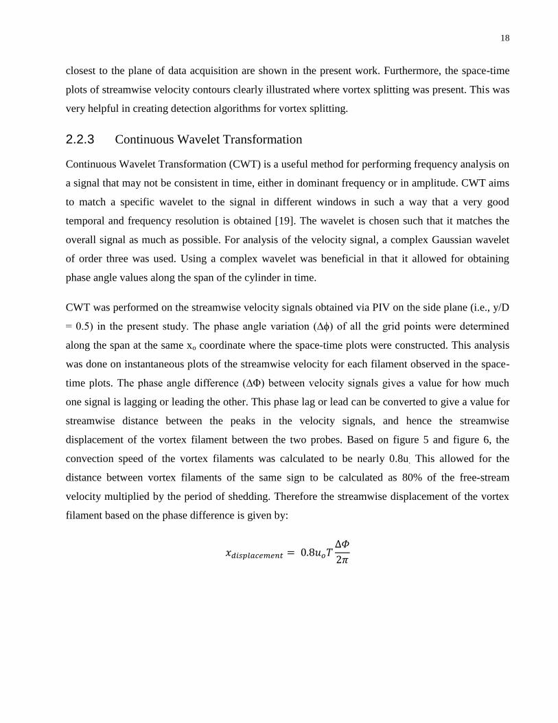
time plots. The phase angle difference (∆Φ) between velocity signals gives a value for how much

one signal is lagging or leading the other. This phase lag or lead can be converted to give a value for

streamwise distance between the peaks in the velocity signals, and hence the streamwise

displacement of the vortex filament between the two probes. Based on figure 5 and figure 6, the

convection speed of the vortex filaments was calculated to be nearly 0.8u. This allowed for the

distance between vortex filaments of the same sign to be calculated as 80% of the free-stream

velocity multiplied by the period of shedding. Therefore the streamwise displacement of the vortex

filament based on the phase difference is given by:

19

A line of best fit on the streamwise displacement of the vortex filament yields the average linear

shape of the filament, giving the average angle (θ) of the vortex filament (see the right side of figure

6). This gives a linear approximation for the angle of the filament, which may hide some of the

features of the filament orientation but gives a good indication of its shape. θ is defined as positive

for counter-clockwise rotations away from the vertical axis. The vortex filament angle was

calculated separately for each vortex filament in the near-wake, and as such the results are presented

for each filament observed.

2.2.4 Fast Fourier Transform and Short-Time Fourier Transform

Velocity signals, obtained from the two constant temperature anemometers in the wake, as explained

in the previous section, had a nearly sinusoidal shape due to the induced velocities from the alternate

shedding of vortices. Fast Fourier Transformation (FFT) of the signals converted this signal from the

time domain to the frequency domain. This was useful in illustrating which frequencies were

dominant in the shedding, as well as their respective amplitudes. The frequency resolution is given

by the ratio of the sampling frequency to the number of samples obtained. Due to the ability to

sample for extended time, 45000 data points were acquired at a sampling frequency of 50Hz, which

allowed for a frequency resolution of 1.1 x 10-3

in FFT analysis.

To observe if the dominant frequency was changing in time, Short-Time Fourier Transformations

(STFT) were applied to the stream-wise velocity signals. STFT breaks the signal into smaller

sections of signal, or windows, before performing the FFT analysis. This allows for observation of

how the frequencies and phases of the vortex shedding changes in time. The size of the window in

STFT, that is how many data points within the window are present, must be chosen to obtain

appropriate temporal and frequency resolution. To obtain high temporal resolution in STFT, a small

window size must be chosen. However, having a small window size reduces the frequency resolution

due to the fact that resolved frequencies are discrete values. Therefore, it is important to ensure that

the window size is chosen such that the dominant Karman frequency is resolved. Otherwise, the

frequency data will have noise that is contributed from the analysis technique.

20

2.2.5 Time Evolution of Phase-Angle Difference Between Two Probes

As explained in section 2.1.4, dual-CTA experiments were performed to acquire simultaneous

velocity signals from two different spanwise locations in the flow. By calculating the phase

difference between these points, it is possible to quantify how oblique the shedding is relative to the

span of the cylinder. The phase angle between the two signals was calculated as a function of time

by means of STFT. The window size for the STFT analysis was chosen such that two shedding

cycles were observed in a single window. The sampling frequency was determined such that the

Karman frequency would be resolved within the window, that is:

Where Fs is the sampling frequency (48Hz), N is the window size (128), Fk is the Karman shedding

frequency (0.75) and the factor 2 ensures that two shedding cycles are present within the window.

The phase angle difference (∆Φ) corresponding to FK between the signals within each window was

calculated and recorded. Due to the fact that ∆Φ was shown to change rapidly in time, each

successive window was chosen to overlap with the previous window. This overlap region covered

7/8 of the window size to yield more continuous phase angle variation in time.

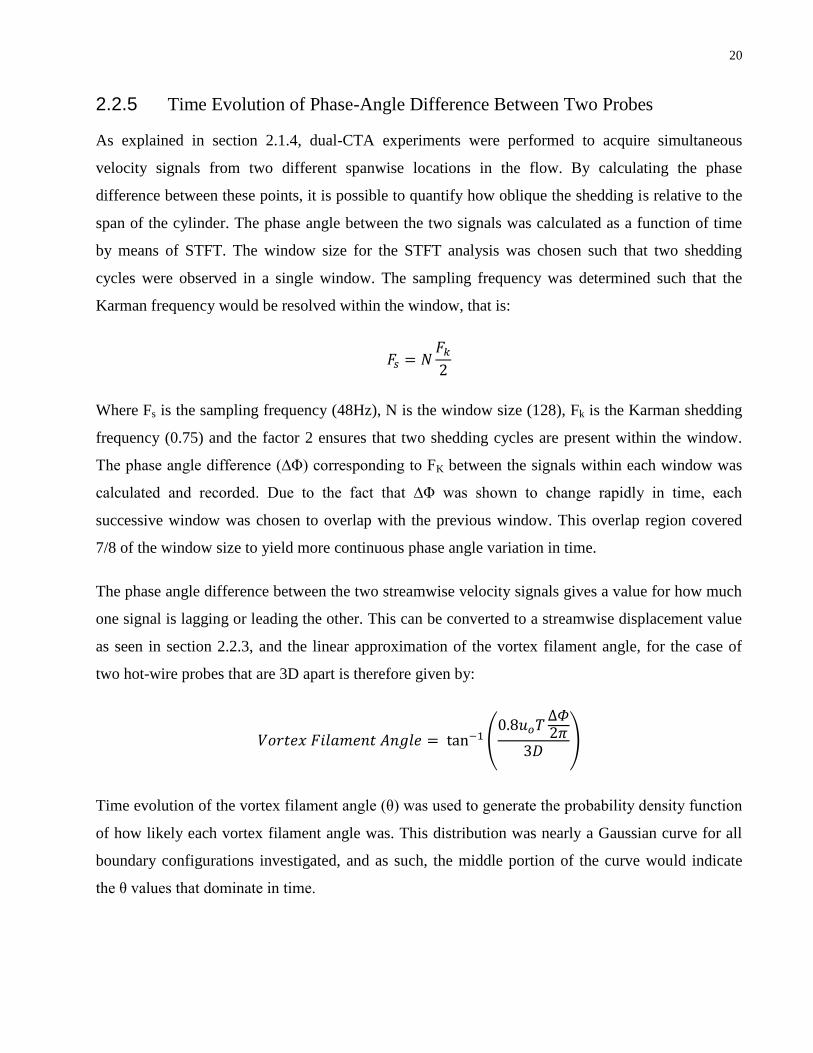
The phase angle difference between the two streamwise velocity signals gives a value for how much

one signal is lagging or leading the other. This can be converted to a streamwise displacement value

as seen in section 2.2.3, and the linear approximation of the vortex filament angle, for the case of

two hot-wire probes that are 3D apart is therefore given by:

(

)

Time evolution of the vortex filament angle (θ) was used to generate the probability density function

of how likely each vortex filament angle was. This distribution was nearly a Gaussian curve for all

boundary configurations investigated, and as such, the middle portion of the curve would indicate

the θ values that dominate in time.

21

All ∆Φ values obtained by STFT analysis were between -π to π. The true value for ∆Φ can be 2π

plus or minus the ∆Φ calculated by the algorithm due to the fact that it is not possible to determine

which direction the phase lag/lead is occurring. To resolve this issue, one experiment setting the two

probes a small spanwise distance (1D) apart was conducted to see what the maximum vortex

filament angle in time is at this Re. For this small separation, it is known that ∆Φ will always be

between -π and π because this corresponds to a vortex filament angle of -63o to 63

o and such large

oblique angles are not possible behind a cylinder. The maximum ∆Φ measured between the probes

that are 1D apart was converted to a maximum vortex filament angle θmax. The θmax was found to be

44.5o, which is constant along the span within a vortex filament such that θmax is the same for both

1D and 3D probe separations. Therefore, this same θmax value can be used to determine the

maximum magnitude of ∆Φ for experiments in which the probes are separated in the spanwise

direction by 3D; ∆Φmax was found to be 1.53π. From there, the correction in the ∆Φ value was done

such that the ∆Φ was allowed to increase or decrease by 2π if the difference in ∆Φ from the previous

value in time would decrease, so long as the absolute value of ∆Φ was less than ∆Φmax calculated

above.

The topic of vortex splitting will be discussed in more detail in section (3.2.3), but for illustrative

purpose, the top right image of figure 13 shows a space time plot of the streamwise velocity that

displays the phenomenon of vortex splitting. The vortex split is shown to initiate at a normalized

time of approximately 25, and the merging of filaments, or hence forth known as branching, is

observed in the subsequent filaments. After the vortex split, a different amount of filaments are

found above and below the spanwise location of the dislocation. The differing amount of vortex

filaments means that during a vortex split, and the corresponding branching, the vortex filament

angle cannot always be calculated with certainty. This is due to the fact that a filament above the

dislocation is connected to two different filaments below the split. Therefore during a split two

different vortex filament angles could be calculated, one with a positive oblique angle and the other

being negative. This uncertainty in θ during regions of splitting leads to variability within the sign of

oblique angles of shedding, and affects the tail regions of the PDFs generated for the different

boundary conditions.

22

Figure 1: The various boundary conditions investigated. a) A cylinder bounded by the channel floor and free-

surface. b) A cylinder bounded by the channel floor and the channel cover. c) A cylinder bounded by a sharp

leading edge geometry endplate on the bottom and the free-surface on top. d) A cylinder bounded an elliptical

leading edge geometry endplate on the bottom and the free-surface on top. e) A cylinder bounded by a sharp

leading edge geometry endplate on both the top and bottom. f) A cylinder bounded by an elliptical leading

edge geometry endplate on both the top and bottom.

Note that FOV in the figure designates the field of visualization and is marked with dotted rectangular

regions, S shows the spanwise length of the cylinder, D shows the diameter of the cylinder and L shows the

distance of the cylinder center from the leading edge of the plate.

23

Figure 2: Schematic detailing the plane on which PIV experiments are being

performed.

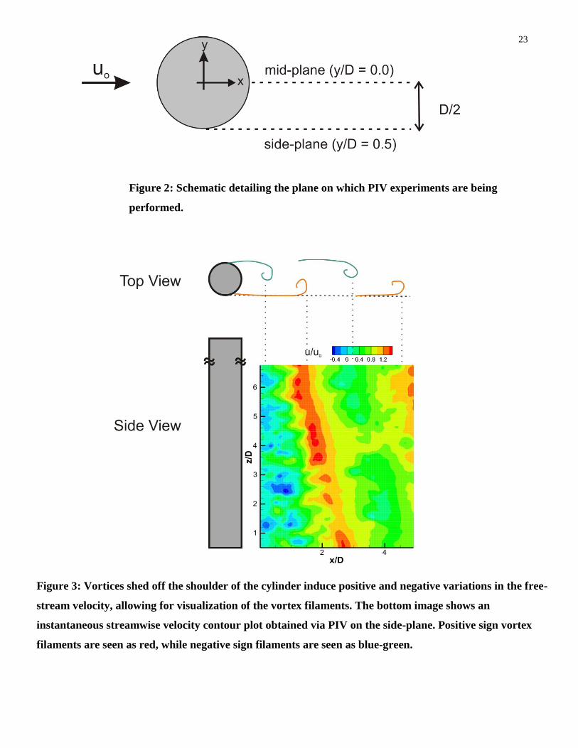
Figure 3: Vortices shed off the shoulder of the cylinder induce positive and negative variations in the free-

stream velocity, allowing for visualization of the vortex filaments. The bottom image shows an

instantaneous streamwise velocity contour plot obtained via PIV on the side-plane. Positive sign vortex

filaments are seen as red, while negative sign filaments are seen as blue-green.

24

Figure 4: Method to determine the length of the recirculation region along the span.

25

Figure 5: Generation of space-time plots of contours of the streamwise velocity in the z-t plane. The z axis (spanwise direction) is

normalized by D and time t is normalized by D/uo. The plot is constructed from the time trace of streamwise velocity signals

obtained in the y/D = 0.5 plane, at a chosen streamwise location (designated as xo) along the entire z direction. The spanwise line

along which the streamwise velocity signals were extracted as a function of time is shown in the figure with the line vector .

26

Figure 6: CWT was used to calculate the phase angle variation along the span based on the instantaneous streamwise

velocity field in the plane of y/D = 0.5. The calculated phase lag along the span is converted to a streamwise distance

(right figure), and the slope of the linear approximation to the curve is converted to an approximation for the vortex

filament angle (θ).

27

Results 3

3.1 Time-Averaged Characteristics of Vortex Shedding

To assess how different end boundary conditions affect the spanwise uniformity of the near wake of

a cylinder in time-averaged sense, velocity vector fields obtained via PIV on the mid-plane of the

cylinder (y/D =0 plane) were analyzed over the range of Reynolds numbers from 104 to 3.6x10

4. As

explained in the preceding chapter, the entire spanwise field of visualization was divided into two

separate regions with a slight overlap to obtain increased vector resolution (see section 2.1.3 for

details), and 4 sets of 200 image pairs were acquired and ensemble averaged for each region in order

to compute the time-averaged streamwise velocity distribution, from which the demarcation line

between the recirculation flow and the downstream flow was calculated along the length of the span

(see section 2.2.1 for details).

The demarcation lines at four different Reynolds numbers are given in figure 7 for the case of a

cylinder bounded by the channel floor at the bottom and the free-surface at the top. Inspection of

these lines show that, except for Re = 104, the demarcation lines at all Reynolds numbers depict

significant spanwise non-uniformity, degree of which increases as the flow Reynolds number

increases. The change in the time-averaged recirculation region becomes more dramatic toward the

free surface. It can, therefore, be concluded that the free-surface boundary condition influences the

spanwise uniformity of the flow greatly at higher Reynolds numbers. Taken as a whole, figure 7

suggests that the flow under the presence of free surface becomes more and more three-dimensional

as the Reynolds number increases.

For cases in which the top end of the cylinder is bounded by either a channel wall or an endplate, the

spanwise uniformity even at higher Reynolds numbers is greatly improved. This inference can

clearly be seen from an inspection of figures 8 to 10, where the time-averaged recirculation length

along the span are given at four different Reynolds numbers for the following end conditions: (i) a

cylinder bounded by the channel floor at the bottom and the channel cover at the top (figure 8), (ii) a

cylinder bounded at both ends by endplates having the sharp leading edge, where the distance

between the leading edge of the plate and the cylinder axis is L = 2.5D (figure 9), and (iii) a cylinder

bounded at both ends by endplates having the elliptical leading edge; for which again the distance

28

between the leading edge and the cylinder is kept at L = 2.5D (figure 10). These plots do not

demonstrate a significant increase in formation length near the top of the cylinder, unlike the free-

surface end condition.

What we have seen so far is that the free-surface boundary condition disturbs flow past a cylinder

significantly at high Reynolds numbers. In figure 11, for a cylinder at Re = 36x103 with free-surface

boundary condition, the time-averaged velocity vectors are superimposed over the time-averaged

streamwise-velocity contours near the free surface. Also, in figure 12 (a) to (c), corresponding plots

are shown for the cases where, at the top boundary of the cylinder, the channel wall, the endplate

with sharp the leading edge, and the endplate with the elliptical leading edge are employed

respectively. Note that for the cases where the top boundary is an endplate, a similar endplate was

also placed on the other side of the cylinder to keep symmetry in boundary condition, and the

cylinder axis is kept at a distance L = 2.5D from the leading edge of both the top and the bottom

endplates. For the case of a cylinder bounded by the free surface on its top (figure 11), there exists a

large downward flow from the water-air interface, while for the configurations where a top wall or a

top endplate is present (figure 12 (a) to (c)), there is no appreciable flow in the spanwise direction.

The downward flow observed in the case of the free-surface type boundary can be attributed to the

large pressure gradient between the suction region at the base of the cylinder and the ambient air. As

Re increases, the base suction at the rear of the cylinder increases, and causes a large dip in the water

height near the rear-top of the cylinder. This decrease in water height and the downward flow from

the free-surface were clearly observed even by bare eyes during the data acquisition process. It is this

downward flow that influences the time-averaged recirculation length near the free surface (i.e., the

demarcation line) and introduces a great spanwise non-uniformity in the near-wake, leading to a

condition that does not properly model an infinite cylinder. Therefore, at higher Reynolds numbers,

it is clear that either a top wall or a top endplate is needed to prevent free-surface effects.

It was observed that at a Reynolds number of 104 all experimental configurations studied in the

present work, even those with a free-surface condition, show a demarcation line that is nearly

parallel to the spanwise axis of the cylinder, implying that the time-averaged vortex shedding at this

Reynolds number is quasi-two dimensional. Although this may be the case, averaging the velocity

vectors in the near-wake greatly hides many of the key details of the flow. The next sections will

29

focus on the Reynolds number of 104 and show that the orientations of the vortex filaments at this

sub-critical Reynolds number have an unsteady nature, and vary in time from being near parallel to

largely oblique for the same boundary conditions. Acquisition of 4 sets of 200 image pairs via PIV

provides a total of 40 shedding cycles at this Reynolds number. As we will see in what follows, 40

shedding cycles do not cover all possible vortex-filament alignments, and as such the time-averaged

PIV results discussed in this section are not fully converged. Furthermore, even if a much larger

sample of PIV data were to be time-averaged, a nearly parallel demarcation line might result in if the

oblique angles in one direction cancel the angles in the opposite direction. Attention is, therefore,

directed in the following section towards the unsteady features of the vortex filaments in order to

investigate the variations of their alignment in time and how often the shedding is oblique compared

to being parallel.

3.2 Unsteady Nature of Vortex Filaments

3.2.1 Visualization of Vortex Filaments

To observe how the orientation of vortex filaments in the near wake changes in time under different

end boundary conditions, velocity vector fields were obtained by PIV on the side-plane of the

cylinder (y/D =0.5 plane) at a Reynolds numbers of 104

for a variety of end configurations. In a

similar manner to the mid-plane PIV experiments presented in the preceding section, the entire

spanwise near-wake field was divided into two separate visualization regions with a slight overlap to

obtain increased vector resolution, and 4 sets of 200 image pairs were acquired for each field of

view. The temporal evolution of the velocity vector fields on the side plane were then used to create

space-time plots of the streamwise velocity component and to estimate the variation of the vortex

filament angle (θ) for each end boundary configuration (see section 2.2.2 and 2.2.3 for details on the

construction of these plots). In figures 13 to 23, the space-time plots of streamwise velocity contours

for four separate sets of PIV data are provided on the top row, and the average vortex filament

angles (θ) corresponding to each filament are given on the bottom row. The space time plots in these

figures display a spanwise field of view only in the top half of the cylinder near wake. The spanwise

field of visualization in the bottom half of the near wake were also studied and were found to show

analogous characteristics. Hence, in order to avoid repetition, only the patterns from the top half of

30

the visualization field are reported in the present work. Nevertheless, the general characteristics

observed were pertinent over the entire spanwise near-wake region behind the cylinder.

Overall examination of figures 13 to 23 show that for all boundary conditions examined, the

orientation of the vortex filaments in the near wake is time dependent. For a given end condition, the

vortex filament is parallel to the cylinder span at one instant in time, while it becomes oblique at

another instant. Furthermore, the direction of obliqueness also largely differ in time, that is, θ values

plotted in the bottom row show a change in time from being positive to negative.

Interestingly, the trends observed for the vortex filament angle in figure 14 is different from the rest:

vortex filament angles are near θ = 0° and show little variability with time for the particular case

where the cylinder is bounded by the channel floor on its bottom end and the channel cover on its

top. To examine if this lack of variability in vortex filament angle is due to the low sample size of

PIV measurements, figure 15 shows the space-time plots of streamwise velocity and the average

angle θ of each filament as a function of time for the bottom half of the cylinder near wake. The θ

values show slightly larger variability in this visualization field, but not to the same level of

variations as shown in other end configurations. Due to the inability to place CTA probes through

the top channel cover however this boundary configuration was limited to only PIV measurements.

Therefore it was not possible to tell whether this lack of variability in vortex filament angle is due

purely to the low sample size obtained by PIV compared to the CTA results to be discussed in the

next section, or is a feature of the flow for this end configuration.

The space-time plots of streamwise velocity contours allowed the quantitative visualization of the

phenomenon called vortex dislocation, also known as vortex splitting, in the near-wake of the

cylinder. The vortex dislocations will be examined in more detail in section 3.2.3, but before closing

this section, we would like to point out how vortex dislocations can be distinguished on the space-

time plots of the streamwise velocity and the corresponding vortex filament θ angle versus

normalized time plots. For example, see the rightmost space-time plot in figure 13: nearly around the

normalized time of tuo/D = 20 the streamwise velocity contours that are indicative of vortex

filaments in the space-time plot show bifurcation between successive vortex filaments of same sign

and different number of vortex filaments above and below the bifurcation (vortex splitting) location.

The corresponding plot showing the variation of the vortex filament angle (θ) with time also shows

31

large angular changes between the two subsequent vortex filaments near the time a split initiates.

These jumps in θ value are due to the bifurcation of the filaments, and that for the same filament

before the branching two different θ values could be calculated, one for each branch. It should be

emphasized that vortex dislocation phenomenon has been observed before via the smoke or dye

visualization of the flow for smaller Reynolds numbers by previous researchers [3], [4]. However,

there have been no studies visually showing the existence of this low-Reynolds number phenomenon

at much higher (subcritical) Reynolds number values due partly to the inability to visualize flow

using such qualitative techniques at high Reynolds numbers. The presence of dislocations at high

Reynolds numbers was suggested from the modulations in pressure/velocity measurements along the

span [7], [13]. Hence, cinema technique of PIV and construction of space-time plots enable the first

visualization of this event at high Reynolds numbers.

The space-time plots of the streamwise velocity presented in the present section showed that

examination of 4 sets of 200 velocity vector fields, in other words roughly 40 shedding cycles, are

not sufficient to properly characterize if and how a given end condition affects the orientations in

which the vortex filaments are shed behind the cylinder or to generalize which shedding angles are

observed the most for different end boundary conditions. The need for acquisition of longer samples

of data necessitated the dual-CTA measurements that will be presented now.

3.2.2 Effect of End Configuration on the Vortex Filament Orientation

Dual-CTA experiments were performed at a Reynolds number of 104 to properly analyze the time

dependency of the vortex filament angles shed in the near-wake of the cylinder for all the end

conditions studied in the present investigation. The CTA probe locations and characteristics are

given in section 2.1.4. Short time Fourier Transformation (STFT) of the streamwise velocity signals,

measured simultaneously at two locations that are 3D apart in the spanwise direction, gave the time-

evolution of phase angle difference, from which the vortex filament angle (θ) was calculated as a

function of time (see section 2.2.5 for details). As the vortex filament angle was time dependent, the

probability density function (PDF) of θ was generated to evaluate the relative likelihood of shedding

orientations for a given end condition.

Figures 24 to 28 show the probability density functions of the vortex filament angle for various end

conditions. Ideal shedding would have a Gaussian like probability density function (PDF) of θ that is

32

centered on θ = 0° and have a distribution over a narrow band of θ values. The former would imply

that the most frequently occurring orientation of the vortex filament is parallel to the cylinder axis,

and the later would entail minimal variability in θ with time. Therefore, end conditions that promote,

quasi-two-dimensional shedding, can systematically be sorted out by examining the distribution of

the probability density function (PDF) of θ.

Figure 24 shows the PDFs of θ for the case of a cylinder bounded by the endplate having sharp

leading edge and the free-surface. Therein, three different leading edge distances (L/D = 1.5, 3 and

5) are compared. The largest leading edge distance considered (L/D = 5) results in a sharp peak at a

θ value of nearly -15o, with almost all the shedding being largely oblique. This clearly demonstrates

a boundary condition that should be avoided if quasi-parallel shedding is to be promoted. On the

other hand, shorter leading edge distances of L/D = 1.5 and 3 achieve a much better situation with

the shedding orientation mostly centered around a smaller θ value of about -5°. Nevertheless, the

shedding at these smaller L/D values is still slightly slanted most of the time.

Figure 25 shows the PDFs for a cylinder bounded by the endplate having elliptical nose on the

bottom and the free-surface on the top for three leading edge distances of L/D = 1.5, 3 and 5. For all

the L/D values considered, the PDF distributions look alike with the most probable θ values slightly

shifted toward negative oblique values.

Figure 26 shows the PDF of θ for the cylinder bounded by the channel floor on the bottom and the

free-surface on the top. The PDF is centered on a θ value of about -5° for this case. A comparison

with figures 24 and 25 shows that even the use of an endplate at the bottom end of the cylinder does

not improve the shedding orientation when the free-surface bounds the cylinder at the top. That is,

PDF distributions are all centered around -5° even when an endplate is used at the bottom at the L/D

value that achieves the most improved filament angle distribution in presence of the free-surface.

The observations so far suggest that to negate the free-surface affect, use of a top endplate might be

necessary. We, therefore, concentrate in the next figures on configurations where both ends of the

cylinder are bounded by endplates.

The probability density functions (PDFs) of θ corresponding to a cylinder bounded at both of its

ends by endplates having a sharp nose are shown in figure 27 for the leading edge distances of L/D =

33

3 and 5. For this case, the distribution of PDF strongly depends on which value of the leading edge

distance L/D is chosen. For L/D = 3, the PDF of θ shows a symmetric distribution about θ = 0°,

while for L/D = 5, the mean of the PDF is non-zero with a value centered on θ = -10°. Hence, in this

case, a leading edge distance of L/D = 3 achieves quasi-parallel shedding conditions and is favored

over L/D = 5.

Figure 28 shows PDFs of θ for a cylinder bounded at both ends by endplates having an elliptical

nose shape. Again, the effect of two leading edge distances are investigated (L/D = 3 and 5). It can

be seen that both L/D values achieve a probability density function that is roughly symmetric about a

mean value of θ = 0°, and hence show that the most probable shedding orientation is parallel.

However, the probably density function depicts a much tighter bound when the leading edge

distance is chosen to be L/D = 5, indicating lesser temporal variability in θ.

The key finding out of the results in the present section is the presence of free-surface influence,

even at a Re of 104. For all cases where the top of the cylinder is bounded by the water-air boundary,

there is a shift in the PDFs away from zero, that is the peak of the PDF is not at θ = 0, and the

distribution is not symmetric about parallel shedding conditions. This implies that it is most likely

that the filaments are being shed at a negative oblique angle. This is similar to the negative angle of

the demarcation line shown at higher Re for flow past a cylinder bounded by the free-surface.

Therefore at a Re of 104 or greater there is a need for either a top endplate or top wall cover to negate

the effect of the free-surface. Overall comparison of figures 24 to 28 shows that the use of endplates

at both the bottom and top ends of the cylinder at certain L/D values achieve a scenario where the

majority of the vortex filaments are shed parallel to the cylinder axis. Furthermore, the leading edge

distance L/D is found to have a much more critical influence on the orientation of vortex filaments

when an endplate with sharp leading edge is being employed (figures 24 and 27) as opposed to an

endplate with elliptical leading edge shape (figures 25 and 28). The use of an endplate having a

sharp leading-edge shape at high L/D values considerably worsened the shedding orientation

compared to the case with even no endplate at all (figure 26). As indicated in section 2.1.2,

Blackmore [16] showed that the nose shape of the endplate controls whether flow separation occurs

at the leading edge of the endplate or not. With an endplate having sharp leading edge, flow at the

leading edge of the endplate shows separation and then a reattachment further downstream, while the

34

elliptical leading edge shape prevents such a flow separation [16]. The location of the cylinder

relative to the separation at the leading edge of the endplates with a sharp nose therefore greatly

affects the two-dimensionality of the flow, while for the elliptical leading edge there is no such

phenomenon.

3.2.3 Vortex Splitting

Previous research shows that a vortex dislocation, or also known as a vortex split, occurs when a

vortex filament branches and merges with the neighboring filaments of same sign. This phenomenon

is thought to be an inherent feature of the flow at Reynolds numbers greater than 5x103 regardless of

end conditions [7]. Visualization of the phenomenon at high Reynolds numbers has not been

possible before due to the inability to use dye/smoke visualization studies at high flow speeds.

For all the different end configurations considered in the present work, examination of the space-

time plots of the streamwise velocity contours visually showed appearance of this phenomenon at

some instant in time at a high Reynolds number value of 104. A compilation of these plots is

presented for different end configurations in Figure 29. Occasional appearance of vortex splitting

phenomenon can be distinguished in all the space-time plots clearly, i.e., there are time intervals

when the vortex filament bifurcates and connects to the neighboring vortex filament of same sign. It

can also be seen in Figure 29 that the location along the span where the filament splits changes in

time for the cases. During the time when the vortex splitting persists a different number of vortex

filaments can be counted in space-time plots above and below the split. For example, let's consider

the left most plot in the top row of figure 29. The location of the split changes in time and it can be

seen that the filaments on top are splitting and merging to two of its neighboring filaments below.

Correspondingly, there are 11 filaments shown at locations below a z/D value of 8, and only 10 at a

z/D value of greater than 10. A further characteristic is that due to the bifurcation of the vortex

filaments, the vortex filament angle θ tends to vary suddenly near the instants when the vortex

splitting arises. Large phase angle variations along the span and consequent jumps in vortex filament

angle θ in time were observed to be key features of vortex splitting. Overall consideration of Figure

29 shows that splitting occurs in some cases when the vortex filament is being shed at a largely

oblique angle, while in other cases it occurs right after a filament shed parallel to the cylinder span.

35

Another common characteristic related to the vortex splitting phenomenon is represented in Figure

30, where time-traces of the streamwise velocity signals obtained via the PIV measurements on the

side-plane (y/D = 0.5 plane) are presented at two points in the flow. These points are selected from

the space-time plot of the streamwise velocity contours such that one of the points is located near the

split location while the other is far away from it. The velocity signals near the split location are

significantly attenuated and somewhat disturbed during the time when the vortex splitting

phenomenon occurs, while the signals away from the split show no significant sign of change in

amplitude during that time. From here, it can be concluded that highly distorted and attenuated

velocity signals distinguish points near the split location.

In order to study the distribution of spectral density of frequencies in the streamwise velocity signals,

time-frequency analysis using Short-Time Fourier transformation (STFT) was performed on

streamwise velocity signals acquired through CTA measurements. This provided the temporal

dependence of the frequencies in velocity signals. In figure 31, a representative time-frequency

spectrogram of a CTA signal for the streamwise velocity outside of the near-wake (as detailed in

section 2.1.4) is provided. A generic characteristic, observed for all the end configurations studied at

Re = 104 is that there exist periods with significant attenuation of the peak spectral amplitudes in the

time-frequency spectrograms (as can be seen in figure 31). Furthermore, in figure 31, the streamwise

velocity u/uo signal over a duration when the peak spectral amplitude is high is compared with the

signal over a duration when the peak spectral amplitude is attenuated. The streamwise velocity u/uo

signal during when the peak spectral amplitude attains high levels in figure 31 resembles the

streamwise velocity signal observed at a point away from the vortex splitting location given in figure

30, whilst the signal corresponding to the attenuation of peak spectral amplitude in figure 31 looks

similar to that by the split location shown in figure 30.

Taken as a whole, figures 29 to 31 imply that a sudden large change in vortex filament angle, a

disturbance in the velocity signal and a reduction in the peak spectral amplitude in time-frequency

spectrogram are all distinctive characteristics of vortex splits. These features can be used to identify

the presence of vortex splits in a flow without the visualization of the flow, such as performing CTA

measurements at two points separated a distance in the spanwise direction. Performing such dual-

CTA measurements, observations from figure 29 were confirmed. That is, splitting is inherent

36

feature of the flow regardless of the end condition used at a sub-critical Re = 104 and it occurs in

general whether the filament previously shed is parallel or oblique. However, evaluation of the

probability density functions of vortex filament angle θ for end configurations where the cylinder

was bounded by a free-surface on top showed higher likelihood of splitting when the filament angle

θ became greater than approximately a value of 25° in the negative direction. These splits were

preceded by a gradual decrease in θ until this largely negative oblique angle was found, after which a

sharp change in θ was observed. For end configurations that promoted parallel shedding there was

no distinct trend of θ value at which the vortex splitting occurred, although if shedding is to become

largely oblique than once again splitting is likely. This once again shows that in a water channel

there are clear free-surface effects even at a Re as low as 104 (see Appendix A for plots and details).

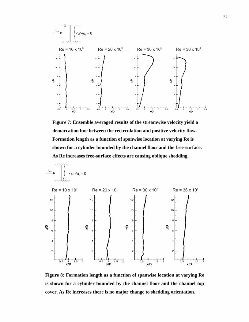
37

Figure 8: Formation length as a function of spanwise location at varying Re

is shown for a cylinder bounded by the channel floor and the channel top

cover. As Re increases there is no major change to shedding orientation.

Figure 7: Ensemble averaged results of the streamwise velocity yield a

demarcation line between the recirculation and positive velocity flow.

Formation length as a function of spanwise location at varying Re is

shown for a cylinder bounded by the channel floor and the free-surface.

As Re increases free-surface effects are causing oblique shedding.

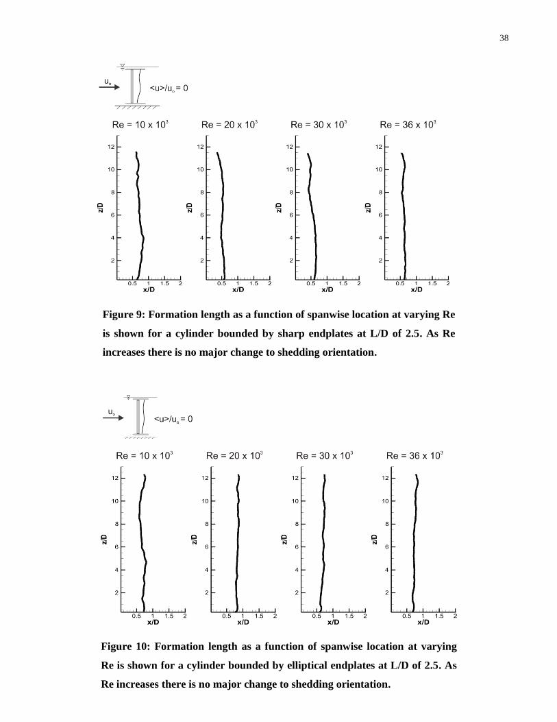
38

Figure 9: Formation length as a function of spanwise location at varying Re

is shown for a cylinder bounded by sharp endplates at L/D of 2.5. As Re

increases there is no major change to shedding orientation.

Figure 10: Formation length as a function of spanwise location at varying

Re is shown for a cylinder bounded by elliptical endplates at L/D of 2.5. As

Re increases there is no major change to shedding orientation.

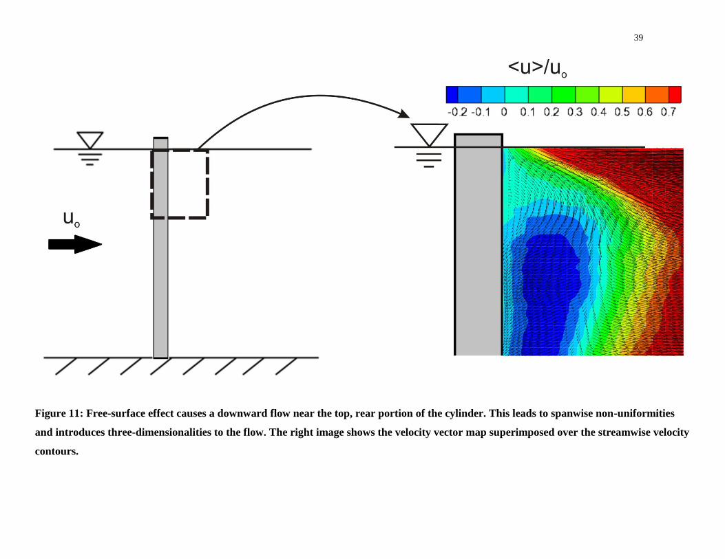
39

Figure 11: Free-surface effect causes a downward flow near the top, rear portion of the cylinder. This leads to spanwise non-uniformities

and introduces three-dimensionalities to the flow. The right image shows the velocity vector map superimposed over the streamwise velocity

contours.

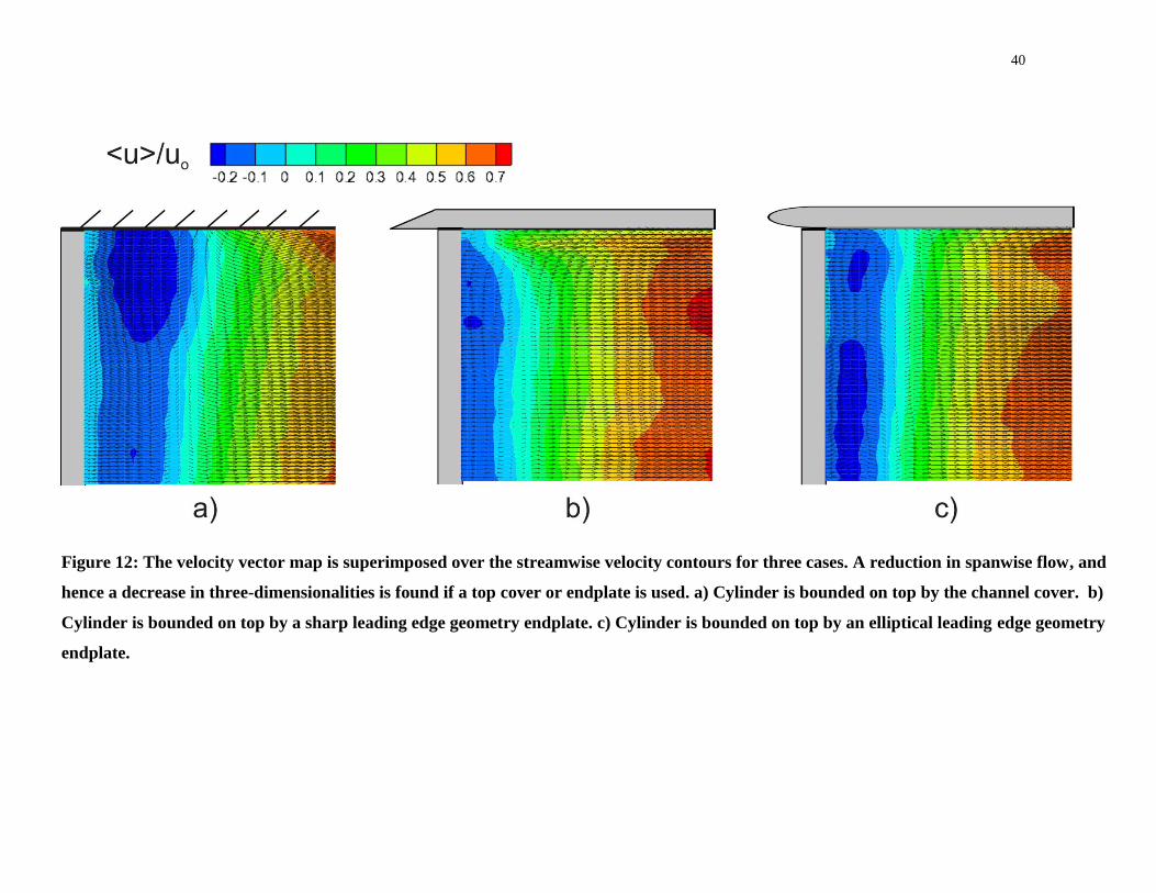
40

Figure 12: The velocity vector map is superimposed over the streamwise velocity contours for three cases. A reduction in spanwise flow, and

hence a decrease in three-dimensionalities is found if a top cover or endplate is used. a) Cylinder is bounded on top by the channel cover. b)

Cylinder is bounded on top by a sharp leading edge geometry endplate. c) Cylinder is bounded on top by an elliptical leading edge geometry

endplate.

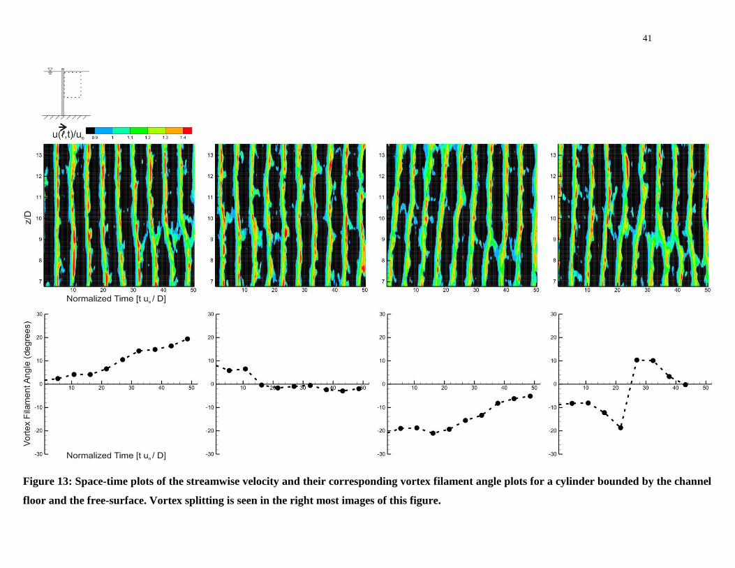
41

Figure 13: Space-time plots of the streamwise velocity and their corresponding vortex filament angle plots for a cylinder bounded by the channel

floor and the free-surface. Vortex splitting is seen in the right most images of this figure.

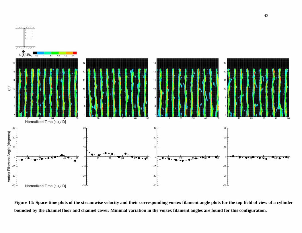
42

Figure 14: Space-time plots of the streamwise velocity and their corresponding vortex filament angle plots for the top field of view of a cylinder

bounded by the channel floor and channel cover. Minimal variation in the vortex filament angles are found for this configuration.

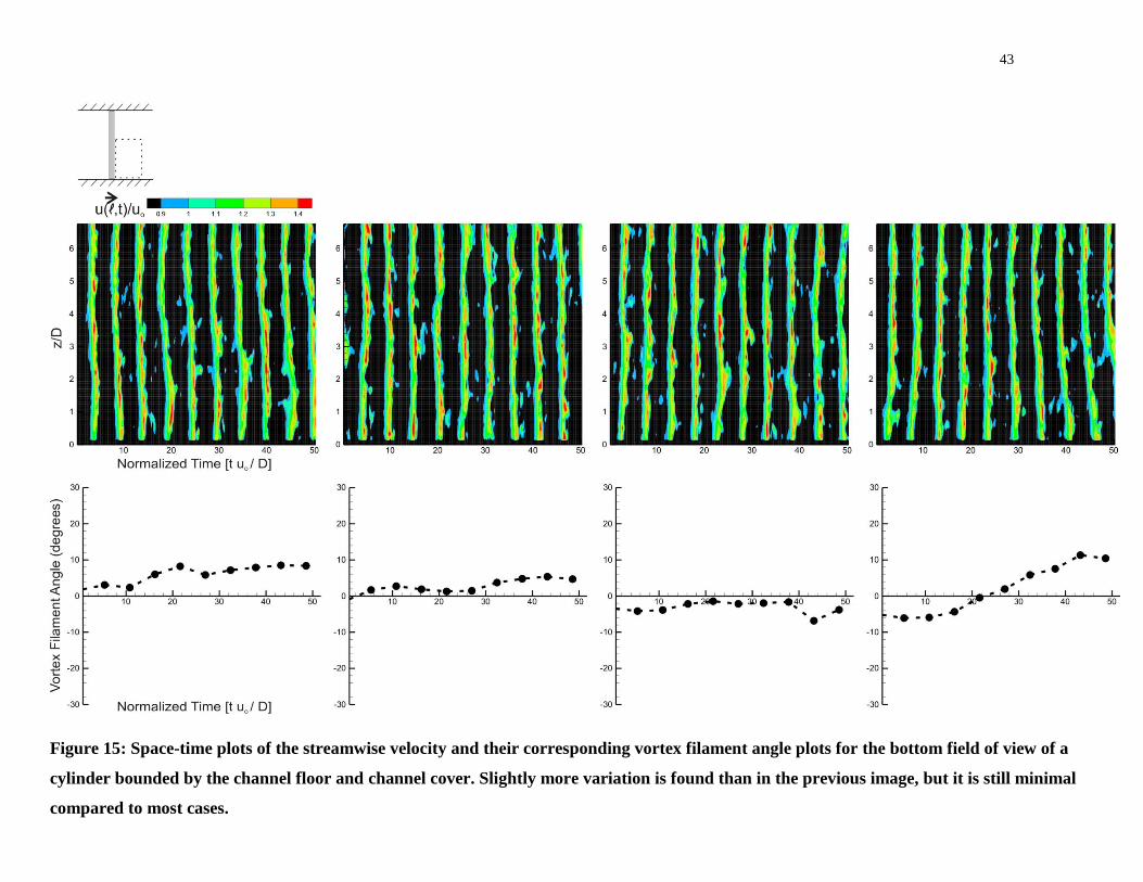
43

Figure 15: Space-time plots of the streamwise velocity and their corresponding vortex filament angle plots for the bottom field of view of a

cylinder bounded by the channel floor and channel cover. Slightly more variation is found than in the previous image, but it is still minimal

compared to most cases.

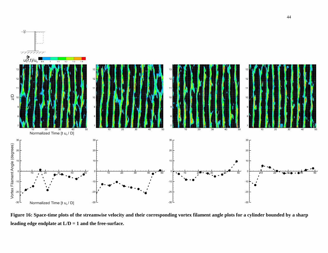
44

Figure 16: Space-time plots of the streamwise velocity and their corresponding vortex filament angle plots for a cylinder bounded by a sharp

leading edge endplate at L/D = 1 and the free-surface.

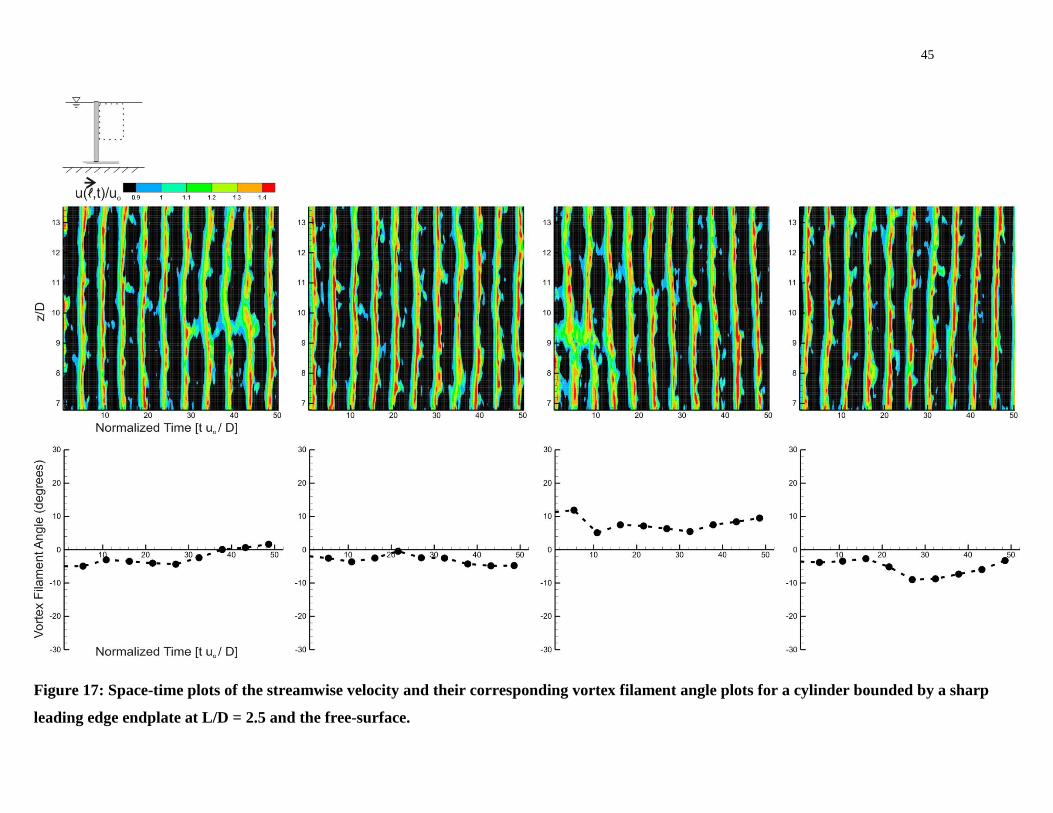
45


leading edge endplate at L/D = 2.5 and the free-surface.

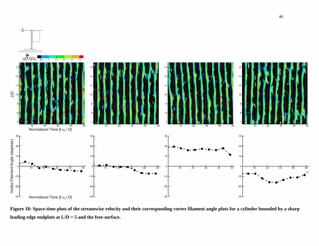
46


leading edge endplate at L/D = 5 and the free-surface.

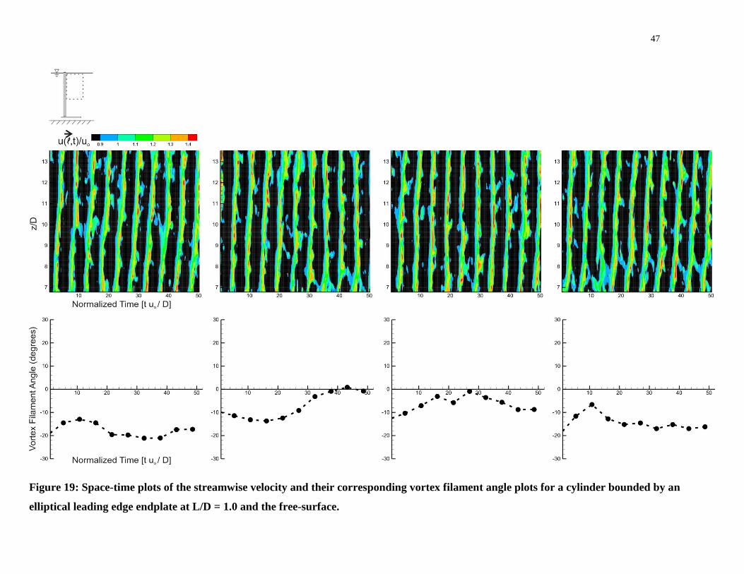
47

Figure 19: Space-time plots of the streamwise velocity and their corresponding vortex filament angle plots for a cylinder bounded by an

elliptical leading edge endplate at L/D = 1.0 and the free-surface.

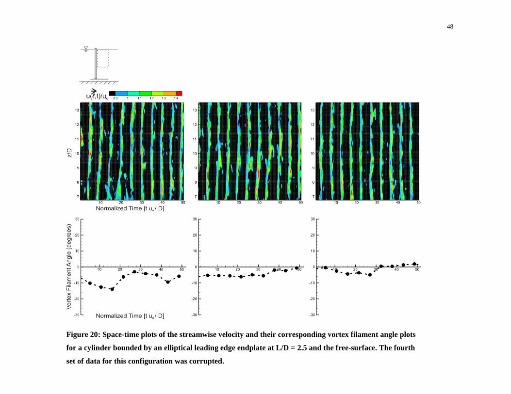
48

Figure 20: Space-time plots of the streamwise velocity and their corresponding vortex filament angle plots

for a cylinder bounded by an elliptical leading edge endplate at L/D = 2.5 and the free-surface. The fourth

set of data for this configuration was corrupted.

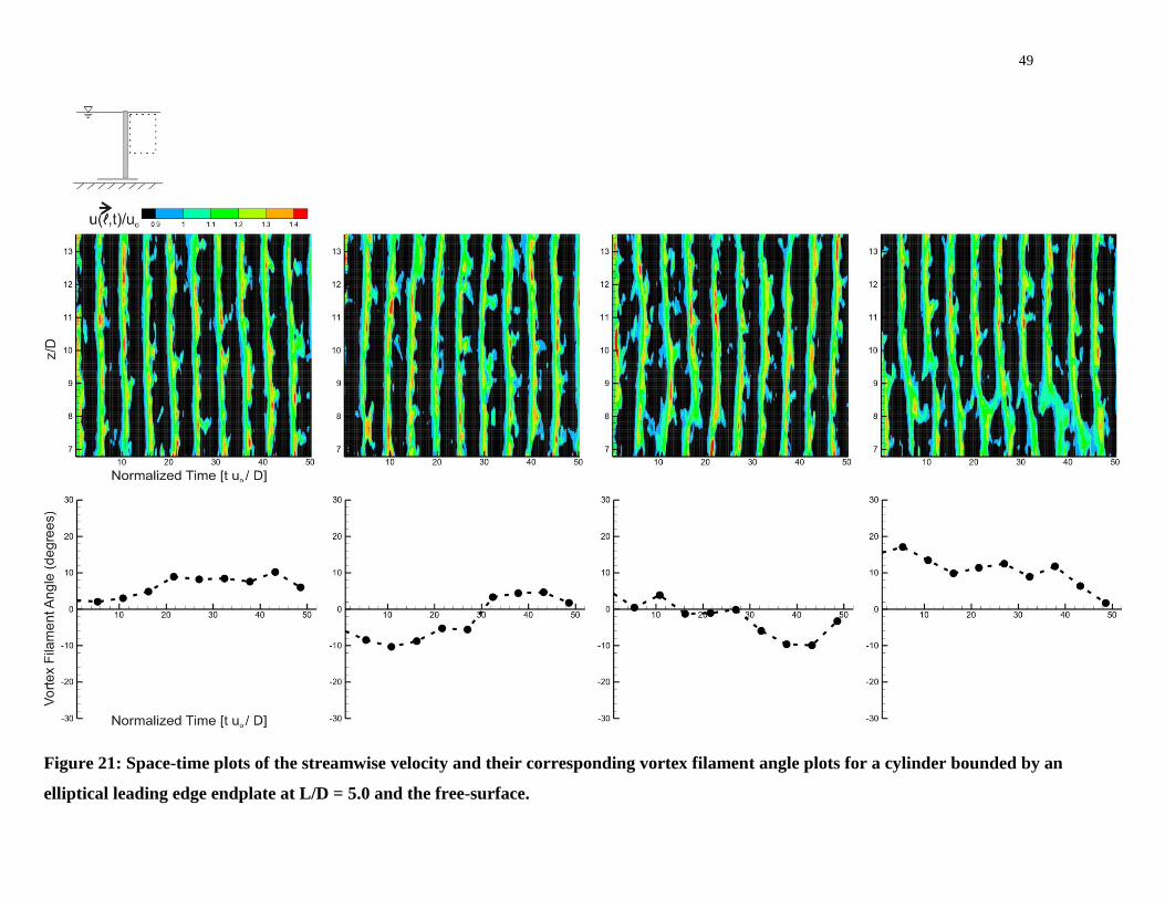
49

Figure 21: Space-time plots of the streamwise velocity and their corresponding vortex filament angle plots for a cylinder bounded by an

elliptical leading edge endplate at L/D = 5.0 and the free-surface.

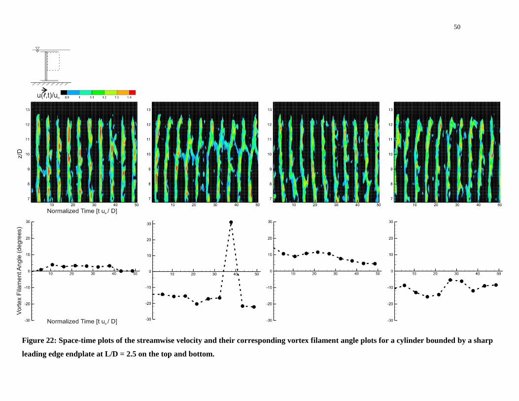
50


leading edge endplate at L/D = 2.5 on the top and bottom.

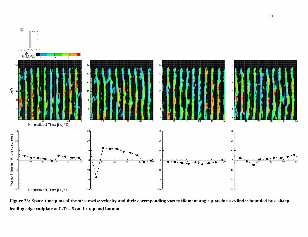
51


leading edge endplate at L/D = 5 on the top and bottom.

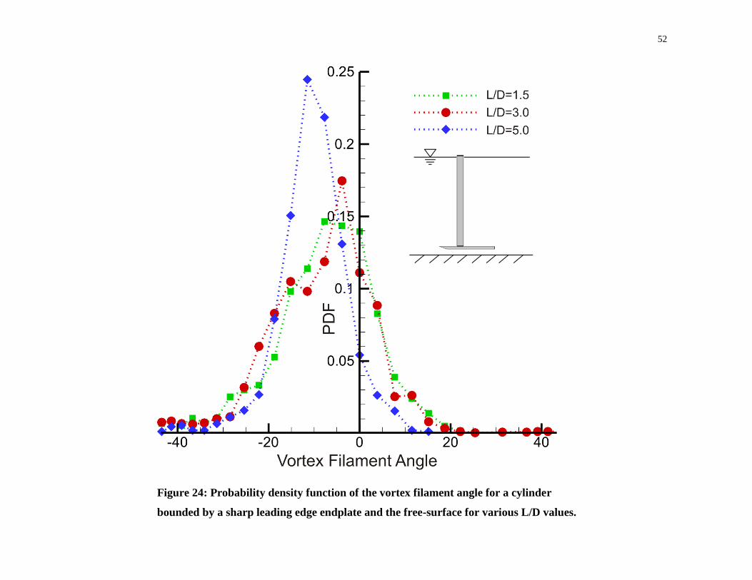
52

Figure 24: Probability density function of the vortex filament angle for a cylinder

bounded by a sharp leading edge endplate and the free-surface for various L/D values.

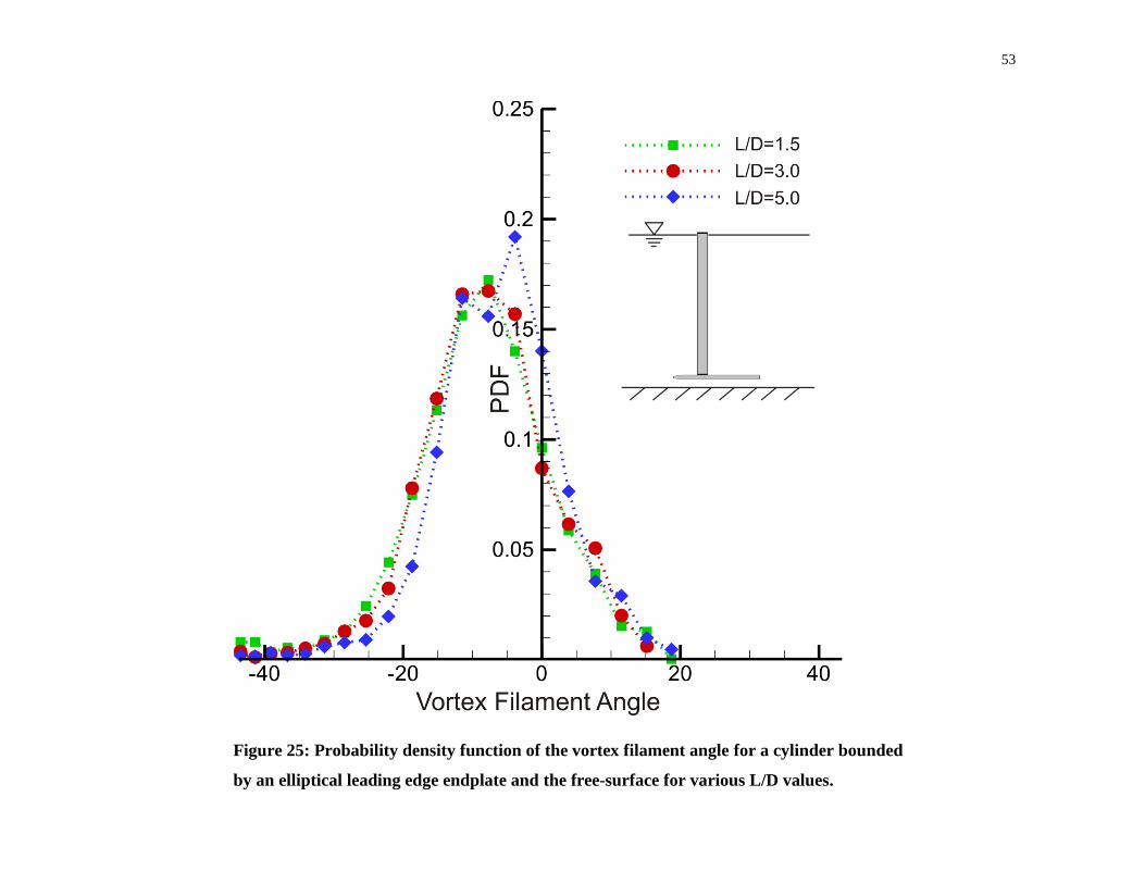
53

Figure 25: Probability density function of the vortex filament angle for a cylinder bounded

by an elliptical leading edge endplate and the free-surface for various L/D values.

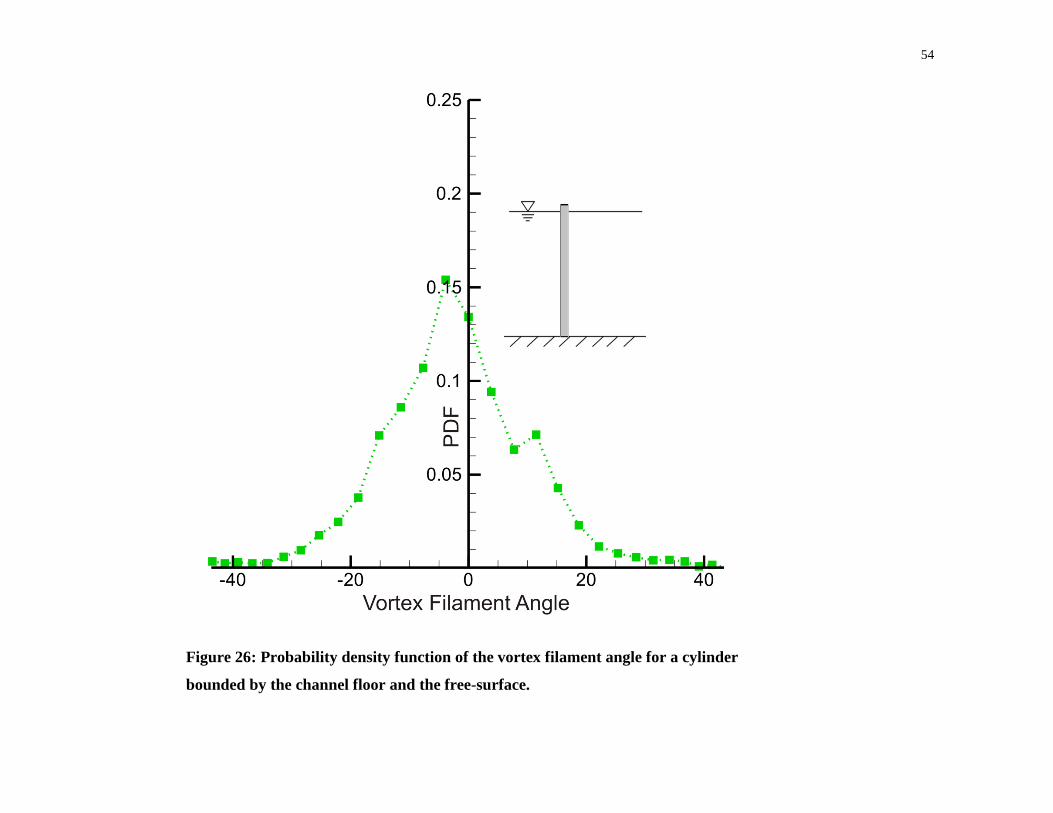
54


bounded by the channel floor and the free-surface.

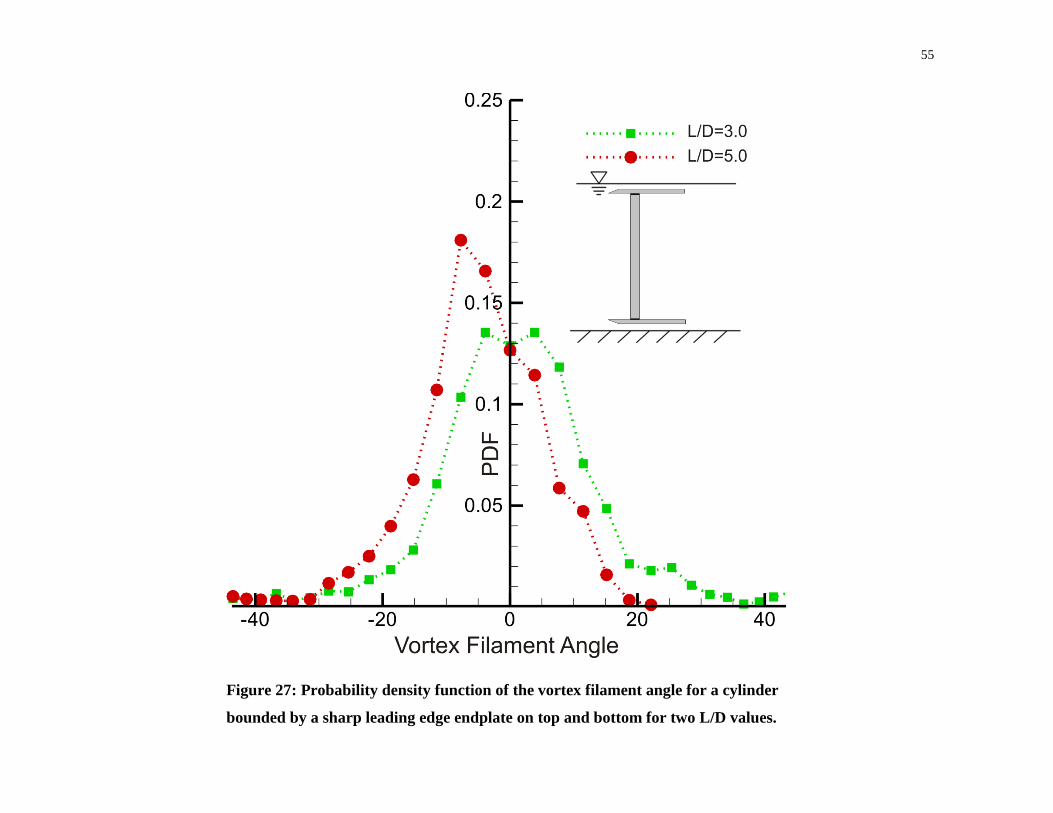
55


bounded by a sharp leading edge endplate on top and bottom for two L/D values.

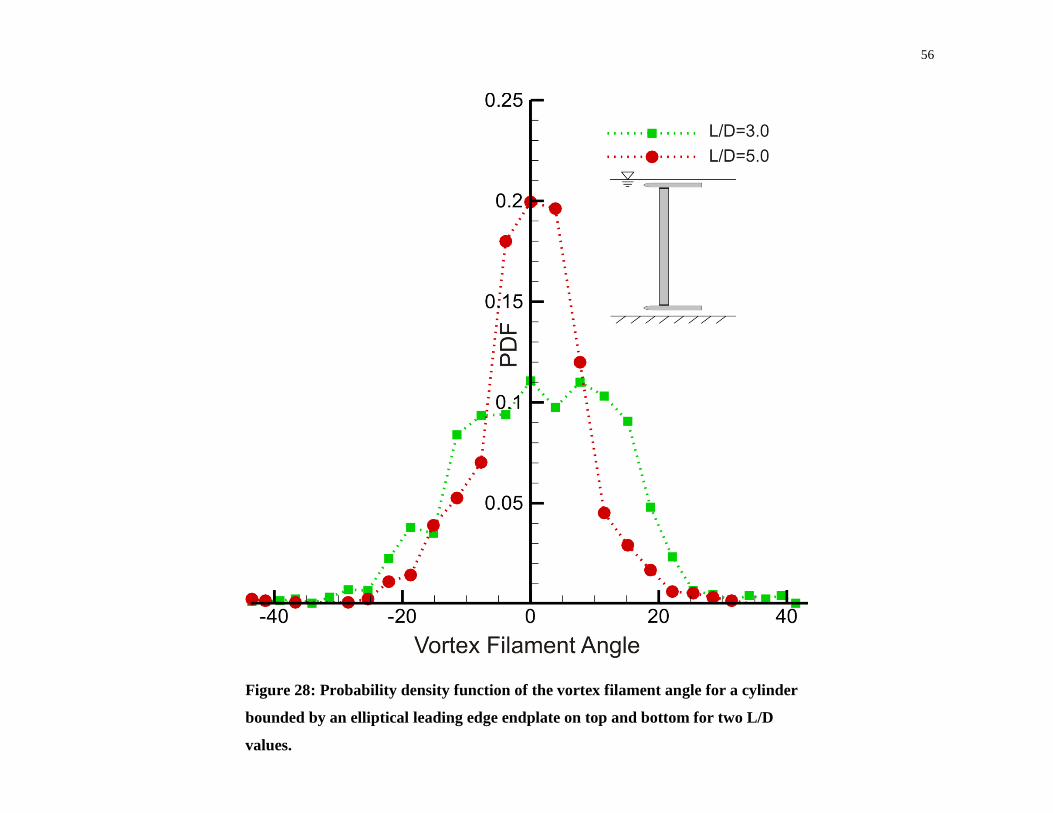
56


bounded by an elliptical leading edge endplate on top and bottom for two L/D

values.

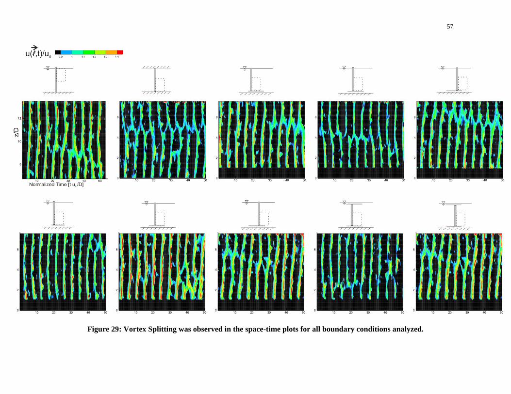
57

Figure 29: Vortex Splitting was observed in the space-time plots for all boundary conditions analyzed.

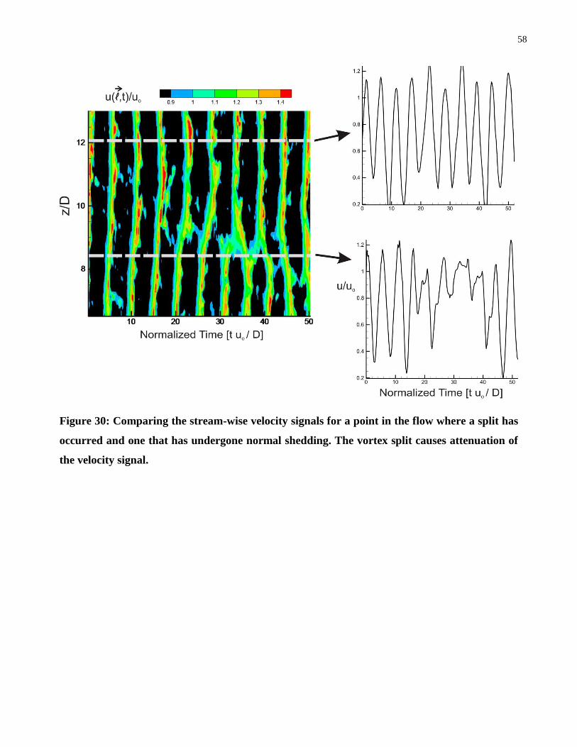
58

Figure 30: Comparing the stream-wise velocity signals for a point in the flow where a split has

occurred and one that has undergone normal shedding. The vortex split causes attenuation of

the velocity signal.

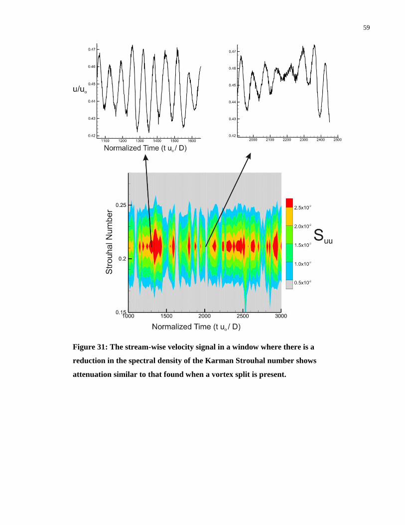
59

Figure 31: The stream-wise velocity signal in a window where there is a

reduction in the spectral density of the Karman Strouhal number shows

attenuation similar to that found when a vortex split is present.

60

Conclusion and Future Work 4

The purpose of this thesis was to develop a method for modeling an infinite cylinder in a finite

experimental setup. This was done by manipulating the boundary conditions of the cylinder to

remove any end effects, which in turn would get rid of any spanwise flow or non-uniformities along

the span. Having quasi-two dimensional flow would allow for researchers to develop near-wake flow

control techniques that would be effective in multiple practical applications, and not in specific

laboratory configurations. Experiments were performed in a free-surface, recirculation water channel

at Reynolds numbers in the sub-critical flow regime, also known as shear-layer transition regime.

Multiple boundary conditions were examined and their effectiveness in creating parallel shedding

was determined. The results obtained by the various experiments undertaken will be summarized in

this section.

Time-averaged analysis of the near-wake of the cylinder showed that as the Re increases, free-

surface effects become more pronounced. For cylinders that were not bounded on top by an endplate

or channel wall, an average negatively oblique angle of shedding was found for flows with a Re

greater than 104. Using a top boundary condition in the form of an endplate or channel wall created

time-averaged shedding that had increased spanwise uniformity, and displayed shedding that was

nearly parallel to the cylinder axis. This is attributed to a reduction in spanwise flow at the top, rear

most portion of the cylinder. When the cylinder is exposed to the free-surface there is a large

mismatch in pressure between the ambient air, and the base pressure of the cylinder, causing a large

spanwise flow behind the cylinder near the free surface. This spanwise flow influences the

formation length at the top of the cylinder and introduces three-dimensionalities in the near-wake.

Analysis of the unsteady nature of the vortex filament angle showed that a cylinder bounded on top

by a free-surface was more likely to have vortex filaments shed at oblique angles even at a Reynolds

number value of 104. Experimental configurations that had the cylinder bounded on top by an

endplate with an appropriate leading edge distance led to shedding orientations that had an average

vortex filament angle θ that was parallel to the cylinder axis, with probability density function of

shedding angles distributed symmetrically about θ = 0°. These results made it clear that free-surface

effects are present for Re greater or equal to 104

and a top endplate or channel cover is needed to

reduce the three-dimensionalities caused by the water-air boundary.

61

Quantitative visualization of the near-wake of the cylinder, with the use of PIV, showed that the

orientation of the vortex filaments varies in time for all the end configurations investigated herein. It

was shown however that using different end boundary configurations for a cylinder leads to different

probability density function (PDF) distributions of the vortex filament angle. Therefore, it was

important to not only determine the average shedding orientation for each boundary condition

examined, but also the variability of the vortex filament angles in time.

Analyzing the probability density functions of the vortex filament angle for different experimental

setups demonstrated how the boundary conditions influence the flow near the mid-span of the

cylinder. For cases in which an endplate with sharp leading edge geometry is used, the streamwise

distance between the leading edge of the endplate and the cylinder axis was shown to be a much

more influential factor than configurations where an elliptical leading edge endplate is employed.

The nose shape was shown to control the flow along the plate previously. According to the

investigation of Blackmore [16] a plate with the sharp nose causes separation at the leading edge,

whilst a plate with the elliptical leading edge removes flow separation. Due to the separation at the

leading edge, the flow at the base of the cylinder for cases in which a sharp endplate is being used is

considerably more dependent on the location of the cylinder along the endplate as opposed to the

endplate with the elliptical leading edge, as the flow over the endplate is less dependent on the

distance from the nose.

One of the most common end configurations used in literature is that of a cylinder bounded by

endplates on top and bottom, at a leading edge distance of three diameters; a configuration

developed by Stansby [8]. Regardless of the shape of the nose, this experimental setup was shown to

induce near parallel shedding, and had a probability distribution that was greatly improved from the

case of a cylinder bounded by the channel floor and free-surface. As the leading edge distance

increased to 5, the use of two elliptical endplates showed markedly improvements in creating

parallel flow while the same configuration with a sharp nose led to oblique shedding due to

separation at the nose of the endplates as mentioned above. It is important to note that all cases in

which the top of the cylinder is bounded by the free-surface show a mean shedding that is negatively

oblique, and the use of an endplate on the bottom does not show discernible improvement regardless

of leading edge distance.

62

Flow visualization showed that there are vortex splits for all boundary conditions examined at a Re

of 104. Vortex splitting is shown to occur regardless of whether the vortex filaments directly before

the split are parallel or oblique to the cylinder axis. This implies that vortex splitting is an inherent

feature of the flow in the sub-critical regime. Although this phenomenon can occur during quasi-two

dimensionality, splitting was found to happen most often when the shedding was largely oblique,

which is similar to what was found at lower Re flows by previous investigators [3], [4].

Future work on the topic can involve determination of the variation of the vortex filament angle for a

cylinder with a large aspect ratio. This would help in understanding how the vortex shedding behind

a near infinite cylinder would vary in time, assisting in creating a model for practical applications.

Furthermore having data for a near infinite cylinder would allow for the observation of vortex

splitting regardless of the aspect ratio.

Further future work can include taking a larger range of leading edge distances for the use of

elliptical leading-edge endplates. This would allow for an optimization of endplate position relative

to the cylinder in generating parallel flow.

Finally, varying the Re of the flow and repeating the experiments that provide the variation in vortex

filament angle would allow for greater insight into the flow dynamics. This would give a more exact

range of values for where the free-surface effects on the mid-span flow are found, as well as helping

to determine in what flow regimes vortex splitting is present.

63

Appendix A

One of the goals of performing the Dual-CTA experiments was to determine if vortex splitting is an

inherent feature of the flow in the sub-critical Reynolds number regime, or if it is due to disturbances

caused by the experimental setup. Section 3.2.3 shows that vortex splitting is found to occur for all

boundary conditions investigated, and also is found regardless of the previous orientation of the

vortex filaments, implying it is an intrinsic feature of this regime. Further analysis will be done in

this appendix to determine the relationship between the end configurations and the orientation of the

vortex filaments prior to shedding.

The PDFs shown in figures 24-28 display the likelihood of the vortex filament angle (θ) for each

boundary condition investigated. All but three of the cases had a PDF that was centered on a non-

zero negative value. Figure 32 shows the value of θ directly preceding a vortex split for all cases in

which the most likely shedding orientation is oblique. Although the data may not be fully converged,

due to a lack of splitting observations in the sample size, there is a clear trend for most cases of θ

being a large negative value before the vortex splits. Figure 33 shows the same results but for the

three cases in which the most likely shedding orientation was parallel. Once again the sample size is

low, but here there is no discernible trend of θ value before a split is found. Furthermore the number

of splits is shown to decrease for cases that promote quasi-two dimensional shedding. This shows

that vortex splitting can be created in the sub-critical regime by causing oblique shedding, but cannot

be removed entirely even if uniform shedding is induced.

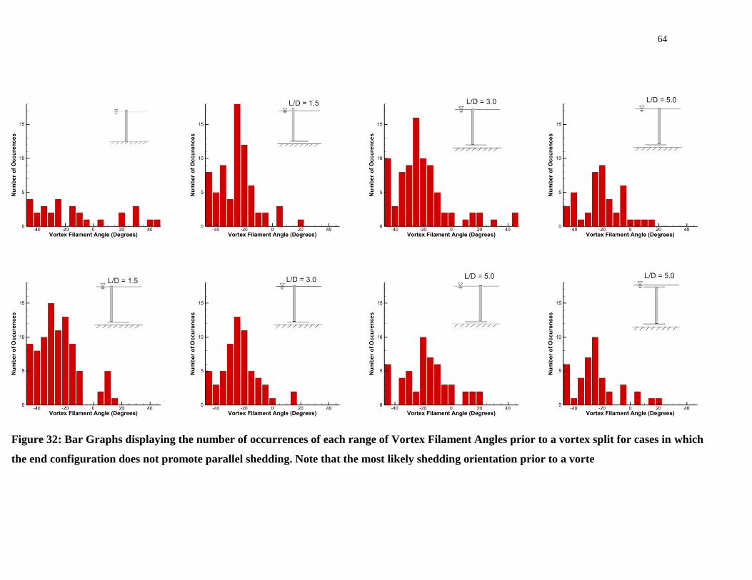
64

Figure 32: Bar Graphs displaying the number of occurrences of each range of Vortex Filament Angles prior to a vortex split for cases in which

the end configuration does not promote parallel shedding. Note that the most likely shedding orientation prior to a vorte

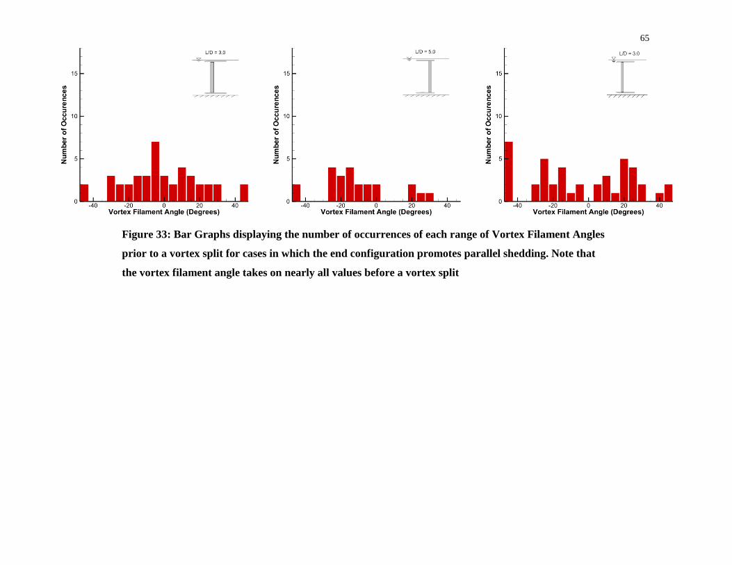
65

Figure 33: Bar Graphs displaying the number of occurrences of each range of Vortex Filament Angles

prior to a vortex split for cases in which the end configuration promotes parallel shedding. Note that

the vortex filament angle takes on nearly all values before a vortex split

66

References

[1] J. H. Gerrard, “The mechanics of the formation region of vortices behind bluff bodies,”

Journal of Fluid Mechanics, vol. 25, pp. 401-413, 1966.

[2] C. H. K. Williamson, “Vortex Dynamics in the Cylinder Wake,” Annual Review of Fluid

Mechanics, vol. 28, 1996.

[3] H. Eisenlohr and H. Eckelmann, “Vortex splitting and its consequences in the vortex street

wake of cylinders at low Reynolds number,” Physics of Fluids, vol. 1, pp. 189-192, 1989.

[4] C. H. K. Williamson, “Oblique and parallel modes of vortex shedding in the wake of a

circular cylinder at low Reynolds numbers,” Journal of Fluid Mechanics, vol. 206, pp. 579-

627, 1989.

[5] M. Hammache and M. Gharib, “A novel method to promote parallel vortex shedding in the

wake of circular cylinders,” Physics of Fluids A: Fluid Dynamics, vol. 1, no. 10, pp. 1611-

1614, 1989.

[6] M. Gharib and M. Hammache, “An experimental study of the parallel and oblique vortex

shedding from circular cylinders,” Journal of Fluid Mechanics, vol. 232, pp. 567-590, 1991.

[7] A. Prasad and C. H. K. Williamson, “Three-dimensional effects in turbulent bluff-body

wakes,” Journal of Fluid Mechanics, vol. 343, pp. 235-265, 1997.

[8] P. K. Stansby, “The effects of end plates on the base pressure coefficient of a circular

cylinder,” Aeronautical Journal, vol. 78, pp. 36-37, 1974.

[9] R. St ger and H. Eckelmann, “The effect of endplates on the shedding frequency of circular

cylinders in the irregular range,” Physics of Fluids, vol. 3, no. 9, pp. 2116-2121, 1991.

[10] T. A. Fox and G. S. West, “On the use of end plates with circular cylinders,” Experiments in

Fluids, vol. 9, pp. 237-239, 1990.

67

[11] S. Szepessy and P. W. Bearman, “Aspect ratio and end plate effects on vortex shedding from

a circular cylinder,” J. Fluid Mech, vol. 234, pp. 191-217, 1992.

[12] S. Szepessy, “On the control of circular cylinder flow by end plates,” European Journal of

Mechanics, B/Fluids, vol. 12, pp. 217-244, 1993.

[13] S. Szepessy, “On the spanwise correlation of vortex shedding from a circular cylinder at high

subcritical Reynolds number,” Physics of Fluids, vol. 6, no. 7, pp. 2406-2416, 1994.

[14] C. Norberg, “An experimental investigation of the flow around a circular cylinder: influence

of aspect ratio,” Journal of Fluid Mechanics, vol. 258, pp. 287-316, Apr. 1994.

[15] R. Narasimha and S. N. Prasad, “Leading edge shape for flat plate boundary layer studies,”

Experiments in Fluids1, vol. 17, no. 5, pp. 358-360, 1994.

[16] A. D. Blackmore, “The Use of End Plates for a Cylinder in Sub-critical Flow Regime,”

University of Toronto, 2011.

[17] D. Farivar, “Turbulent uniform flow around cylinders of finite length,” American Institute of

Aeronautics and Astronautics, vol. 19, pp. 275-281, 1981.

[18] M. Raffel, C. E. Willert, S. T. Wereley, and J. Kompenhans, Particle Image Velocimetry.

2007.

[19] M. Farge, “Wavelet transforms and their applications to turbulence,” Annual Review of Fluid

Mechanics, vol. 24, pp. 395-457, 1992.

Documents

The Influence of End Conditions on Vortex Shedding from … · The Influence of End Conditions on Vortex Shedding from a Circular Cylinder in Sub-Critical Flow ... 2.2.4 Fast Fourier