The Information Content of Dividend Decreases: Earnings or Risk News?

Doron Nissim Columbia University

Graduate School of Business 3022 Broadway, Uris Hall 604

New York, NY 10027 (212) 854-4249, dn75@columbia.edu

February 2005

I thank Geert Bekaert, Lawrence Glosten, Gur Huberman, Partha Mohanram, Stephen Penman, Douglas Skinner, Jacob Thomas, and seminar participants at Columbia University and the Interdisciplinary Center for helpful suggestions and comments.

The Information Content of Dividend Decreases: Earnings or Risk News?

Abstract

This paper demonstrates that dividend cut announcements convey new information

regarding earnings in the current and subsequent year. While dividend decreases are also associated with an increase in firm risk, the change in risk occurs prior to the dividend announcement. Consistent with these findings, the abnormal stock return during the three-day dividend cut announcement window is approximately equal to the present value of unexpected current and next year’s earnings.

1

I. Introduction

Dividend cut announcements trigger substantial negative returns (e.g., Aharony and

Swary (1980), Michaely et al. (1995)). Yet, prior research generally finds that dividend

reductions are unrelated to future earnings after controlling for current earnings (e.g., Healy and

Palepu (1988), Benartzi et al. (1997), Nissim and Ziv (2001)).1 Several recent studies interpret

this evidence as indicating that dividend decreases do not convey new information about future

earnings but rather imply an increase in firm risk (e.g., Benartzi et al. (1997), Allen and

Michaely (2002), Grullon et al. (2002), Grullon et al. (2003), Chen et al. (2004)). This study

provides new evidence on the earnings and risk implications of dividend cuts. In particular, I

show that essentially all of the market response to dividend cut announcements is due to new

information about current and next year’s earnings, and that little if any risk information is

conveyed by these announcements.

The differences between the findings of the current and prior studies are due primarily to

methodological choices. Specifically, I use alternative approaches for measuring earnings

expectations and examine changes in risk premiums using short rather than long intervals. While

these choices potentially involve trading-off one bias for another, I provide evidence that

supports my choices and demonstrate their impact on the results. In particular, I document the

sources and extent of bias associated with using different methodologies for measuring expected

earnings. I also show that using long intervals for estimating risk disguises the fact that

essentially all of the increase in the riskiness of dividend cut firms occurs before the dividend

announcement. Finally, I demonstrate that my estimates of the magnitudes of earnings and risk

news conveyed by dividend cut announcements are consistent with observed market responses.

1 One exception is DeAngelo et al. (1992). Focusing on firms with positive earnings and dividends in the prior ten years and a loss in the current year, DeAngelo et al. (1992) find that those firms that cut their dividends in the current year report lower next year earnings even after controlling for current year earnings.

2

The study proceeds as follows. Section II discusses difficulties and trade-offs involved in

measuring expected earnings for dividend decrease firms. Section III develops the methodology

used to examine the future earnings implications of dividend cuts. Section IV describes the

sample, and Section V presents the empirical findings of the earnings and risk analyses. Section

VI concludes the paper.

II. Issues in Measuring Earnings Expectations for Dividend Decrease Firms

To examine the future earnings implications of dividend change announcements,

previous studies regress future earnings on the dividend change, current earnings (i.e., earnings

in the year during which the dividend change occurs) and proxies for expected future earnings.

They then use the estimated coefficient of the dividend change as a measure of the information

content of dividends. Current earnings are included in the regression because they help explain

future earnings and are partially predictable at the time of the dividend change (e.g., using

information from intermediate quarterly reports or from the financial press). As many of these

studies recognize, however, this choice induces bias against finding information content in

dividends because current earnings, which are only partially known at the time of the dividend

announcement, are positively related to the dividend change. Thus, the decision to control for

current earnings potentially involves trading-off bias against versus towards accepting the

information content of dividends hypothesis.

How important is this choice? According to Miller and Rock (1985), this issue is at the

core of the information content of dividend hypothesis. Miller and Rock argue that dividend

changes convey information about future earnings indirectly by changing the market’s estimate

of current earnings, which in turn contributes to the estimate of future earnings. Thus, if dividend

decreases predict lower current earnings, which in turn imply lower future earnings, the negative

3

future earnings implications of the dividend change will be captured by the coefficient of current

earnings rather than by the dividend coefficient. In other words, controlling for current earnings

exposes the analysis to the risk of “throwing the baby out with the bathwater.”

The Miller and Rock argument applies both to dividend increases and decreases. But

controlling for current earnings may introduce an additional bias which is unique to dividend

decreases. To the extent that dividend cut firms are more likely to recognize negative “special

items,” their earnings will be less persistent than those of other firms.2 If this is not incorporated

in the analysis, the model will overstate the persistence of the negative shock to earnings in the

dividend decrease year, leading to an understatement of expected future earnings. Accordingly,

unexpected earnings (i.e., realized earnings minus expected earnings) of dividend decrease firms

will be overstated, and this bias may offset the negative earnings implications of dividend cuts.

Negative special items may be more prevalent for dividend decrease firms due to two

accounting phenomena: conservatism and “big bath.” Conservatism is an accounting convention

which requires the recognition of anticipated losses, such as those due to impairment of assets or

restructuring of operations. Thus, if dividend reductions signal lower future cash flows, they

should be associated with impairment losses, restructuring charges and other negative special

items. The big bath effect is related to management behavior. Theoretical, empirical and

anecdotal evidence suggests that in the presence of bad news (such as those causing a dividend

cut), managers often choose to take a “big bath;” that is, they overstate estimated liabilities such

as accrued restructuring costs or they write down assets.3 These charges are generally not

2 Skinner (2003) shows that the persistence of earnings is positively related to the level of dividends, especially for low levels of dividends. That is, low dividend firms have particularly low earnings persistence. This evidence suggests that dividend decrease firms may also have low earnings persistence. The current study examines this conjecture by focusing on the magnitude of transitory earnings.

4

expected to recur in future periods and are typically classified as “special items.” I next discuss

the methodology used in this study to mitigate these biases in measuring expected earnings.

III. Methodology

With a perfect measure of expected earnings immediately prior to the dividend

announcement, testing whether dividend cuts convey new earnings information is

straightforward; one only needs to calculate the t-statistic of the mean difference between

realized and expected earnings for a sample of dividend decrease firms. Equivalently, one could

run the following regression:

EPS(t)/P = E[EPS(t)]/P + λ DIV_DEC + ε, (1)

where EPS(t) is earnings per share in year t (t = 0, 1, 2, …), E[.] is the expected value operator

conditioned on publicly available information prior to the dividend announcement (in year 0), P

is price per share prior to the dividend announcement, and DIV_DEC is a qualitative variable

indicating a dividend decrease. Realized and expected earnings per share are deflated by price

per share to mitigate heteroscedasticity since the standard deviation of EPS is approximately

proportional to price (e.g., Baker and Ruback (1999)).

Unfortunately, E[EPS(t)] is unobservable. I therefore estimate this quantity using

information from two market-based proxies for expected earnings: analysts’ forecasts and price

per share. Specifically, I model expected EPS as follows:

E[EPS(t)] = β ECR(t) × P + δ AF(t), (2)

where ECR(t) (Earnings Capitalization Rate) is a proxy for the rate at which investors capitalize

expected EPS(t) into price, and AF(t) (Analysts’ Forecast) is a measure of available analysts’

3 For examples of anecdotal, empirical, and analytical evidence, see Jacksonth and Pitman (2001), Elliott and Hanna (1996) and Kirschenheiter and Melumad (2002), respectively.

5

EPS forecast for year t at the time of the dividend announcement. Both analysts’ forecasts and

price reflect expectations of market participants regarding future earnings. However, prior

research establishes that both measures are somewhat inefficient and biased, and that each

contains incremental information relative to the other.4 Thus, by incorporating information from

both measures, equation (2) may generate a more efficient estimate of expected earnings than

estimates based on price or analysts’ forecasts alone.

The rate at which investors capitalize expected earnings, ECR(t), is a function of

macroeconomic variables (e.g., interest rates, market risk premium) as well as firm-specific risk,

expected growth and payout.5 I therefore specify ECR(t) as a linear combination of the following

variables:

ECR(t) = αyear + αindustry + αdistance + α1 BETA + α2 VOLAT

+ α3 LEV + α4 SIZE + α5 BM + α6 GROWTH + α7 YIELD, (3)

where αyear is a year fixed effect, included to capture the average effect of macroeconomic

variables; αindustry is an industry (2-digit SIC) fixed effect, which controls for industry-specific

risk and growth prospects; and αdistance is a fixed effect which controls for the number of months

between the dividend announcement and the end of the fiscal year. This latter effect is important

because the present value of earnings depends on the length of time until their realization.

The continuous variables in equation (3) are commonly used measures of risk, expected

growth and payout. BETA is a measure of systematic risk, estimated from monthly stock returns

4 For a review of this literature, see Kothari (2001). Note that the precision of the price-based measure of expected earnings is affected by the quality of the empirical proxy for ECR(t) in addition to price efficiency. Similarly, analysts’ forecasts may contain error due to their discrete nature (i.e., they may be stale at the time of the dividend announcement) in addition to error due to analysts’ inefficiencies in processing information. 5 For example, under the Gordon (1962) model, ECR(1) = (r – g) / d, where r is the cost of equity capital, g is expected growth, and d is the dividend payout. For empirical specifications of ECR models, see Beaver and Morse (1978), Zarowin (1990), Fairfield (1994), and Greenspan (1997).

6

and the CRSP value-weighted returns during the five years that end in the month prior to the

dividend announcement. VOLAT reflects idiosyncratic risk and is measured as the root-mean-

squared error from the BETA regression. LEV, the ratio of total liabilities to the sum of total

liabilities and the market value of equity, is a proxy for financial risk. SIZE (log of market value

of equity) and BM (book-to-market ratio) capture risk and growth prospects. GROWTH is a

measure of analysts’ long-term earnings growth forecast available at the time of the dividend

announcement. YIELD is the ratio of the indicated annual dividend (the most recent quarterly

dividend times four) divided by closing price two days prior to the dividend announcement.6

I next substitute equation (3) into equation (2) and divide both sides by price:

E[EPS(t)]/P = γyear + γindustry + γdistance + γ1 BETA + γ2 VOLAT + γ3 LEV

+ γ4 SIZE + γ5 BM + γ6 GROWTH + γ7 YIELD + δ AF(t)/P (4)

Finally, I substitute equation (4) into equation (1):

EPS(t)/P = γyear + γindustry + γdistance + γ1 BETA + γ2 VOLAT + γ3 LEV+ γ4 SIZE

+ γ5 BM + γ6 GROWTH + γ7 YIELD + δ AF(t)/P + λ DIV_DEC + ε (5)

To test whether dividend decreases provide new information about current (t = 0) and future (t =

1, …,5) earnings, I estimate equation (5) for a sample of dividend paying firms which includes

dividend increases, dividend decreases, and no-change observations. Thus, the coefficient on the

DIV_DEC indicator variable reflects the incremental earnings associated with dividend

decreases. I focus on dividend paying firms because the magnitudes of bias and error in the

6 I use the yield rather than the payout because earnings are negative or close to zero for many dividend decrease firms. Moreover, to the extent that price is a proxy for “permanent earnings,” the yield is likely to be a better proxy for expected future payout than the actual payout due to the stability of dividend payments.

7

proxies for expected earnings may be different for these firms compared to firms that do not pay

dividends.7

While it is impossible to remove all error and bias from the proxies for expected earnings,

it is important to note that the ECR(t) variables (equation (3)) not only improve the precision of

the price-based proxy for expected earnings, but also mitigate potential biases due to

inefficiencies in analysts’ forecasts. For example, prior research documents that the bias in

analysts’ forecasts decreases as the earnings announcement date approaches. Thus, the inclusion

of αdistance in the regression (fixed effect for the number of months until the end of the fiscal year)

mitigates potential bias due to systematic variation in the relative frequency of dividend

decreases during the fiscal year.

Most firms pay dividends on a quarterly basis, so the same annual earnings may be

associated with up to four observations. The resulting overlap in observations has little effect on

the DIV_DEC coefficient because very few firms have more than one dividend reduction in any

given year (results are not sensitive to the exclusion of these observations). Also, even for

overlapping observations, the values of the dependent variable are not identical because price

(the deflator) is measured at different points in time (reflecting all information up to the

particular dividend announcement). In any case, to mitigate the effect of autocorrelation in the

residual due to overlapping information, I report Newey and West (1987) t-statistics with three

lags.

7 Firms that do not pay dividends are typically small with low profitability and strong growth opportunities (see Fama and French (2001)).

8

IV. Data

The initial sample includes all dividend events in the CRSP files that satisfy the following

criteria: (1) the company paid an ordinary cash dividend (U.S. dollars) in the current quarter and

in the previous quarter, (2) no other distributions were announced between the declaration of the

previous dividend and three days after the declaration of the current dividend, (3) there were no

ex-distribution dates between the ex-distribution dates of the previous and current dividends, and

(4) the indicated annual dividend yield prior to the dividend announcement is at least 0.5%.

Criteria (2) and (3) help ensure that only “clean” dividend changes that avoid confounding

effects from other distributions are identified. Criterion (4) is set to restrict the sample to firms

that pay significant dividends.

For each of the dividend events, I extract from CRSP the monthly stock returns in the

prior sixty months and calculate the BETA and VOLAT measures discussed above (at least 30

return observations are required). Next, I match the dividend event sample with forecast and

reported data extracted from the IBES Detail, Summary and Actual files. The Detail file contains

analyst-by-analyst estimates, while the Summary file contains the consensus (mean and median)

analysts’ forecasts in each month. According to IBES, the Detail file is a reconstruction of

archived data and may therefore contain errors and omissions. Individual analyst forecasts may

also be less precise than the consensus estimates. I therefore use the consensus (mean) forecasts

in the primary analysis, but check the sensitivity of the results to the use of individual forecasts.

Specifically, I rerun all analyses using the most recent EPS and growth forecasts available at

time of the dividend change and report the results of these tests in a robustness section below.

The Summary IBES file consists of chronological snapshots of consensus earnings

forecasts taken on the Thursday before the third Friday of every month. According to IBES, the

consensus forecasts are made available in the following week. I therefore match dividend

9

announcements occurring after the fourth Sunday of each month and before the fourth Monday

of the following month with the consensus forecasts for that month. I require that the following

variables be available from IBES: mean analysts’ EPS forecast for the current (AF(0)) and next

year (AF(1)), as well as mean long-term earnings growth forecast (GROWTH).8 According to

IBES, the long-term earnings growth forecast generally refers to a period of up to five years

ahead. I therefore generate forecasts for earnings in future years 2 through 5 by applying the

mean long-term growth forecast to the mean forecast for the prior year in the horizon; i.e.,

AF(t+s) = AF(t+s-1) × (1 + GROWTH), for s = 2, 3, 4, 5.

The resulting sample is then matched with the COMPUSTAT files by assigning each

dividend event to the earliest fiscal year for which earnings have not yet been disclosed. That

year is designated as year 0. Dividends are often announced simultaneously with quarterly

earnings, with a positive correlation between the two disclosures (e.g., firms are likely to

increase dividends following earnings increases; see, e.g., Benartzi et al. (1997)). To assure that

the dividend events reflect only dividend information, I exclude observations for which the

dividend announcement occurs within three calendar days before or after a quarterly earnings

announcement.9 I next extract the required financial statements information from COMPUSTAT

and delete observations with missing values for current earnings or for any of the explanatory

variables of equation (5) (observations with missing values for future earnings are retained, to

avoid survivorship bias). Finally, to mitigate the effect of influential observations, the variables

are winsorized at the 1th and 99th percentiles of their empirical distributions.10

8 To prevent duplication, I do not include forecasts with “secondary” flag. I adjust all per share numbers for stock splits and stock dividends using the IBES adjustment factor. If the firm is followed on a diluted basis, I use the IBES dilution factor to convert per share variables to a primary basis. 9 Earnings announcement dates are extracted from the quarterly COMPUSTAT files.

10

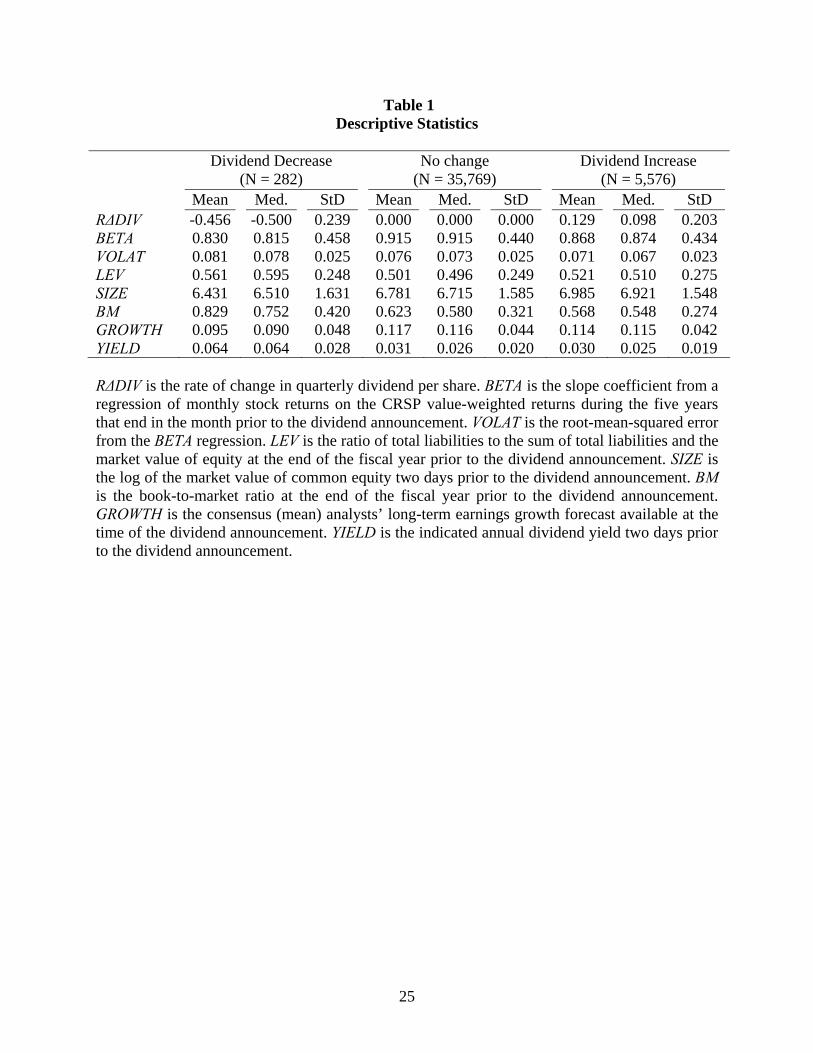
Table 1 presents descriptive statistics for the final sample. As reported, there are 282

dividend decreases, 5,576 dividend increases, and 35,769 no-change announcements that satisfy

all the above criteria. These dividend declarations occurred during the years 1982 through 2003

(IBES data are available since the early 1980s). While dividend reductions are much less

common than dividend increases, they are considerably larger in magnitude—the mean

percentage change in dividends per share is –45.6% for dividend decreases and 12.9% for

dividend increases. Dividend decrease firms are relatively small and have large book-to-market

ratios, financial leverage and residual volatility, suggesting that they are more risky than other

dividend paying firms. However, the average beta of dividend decrease firms is smaller than that

of other dividend paying firms. In addition, dividend decrease firms have substantially smaller

analysts’ long-term growth forecasts and higher dividend yields.

V. Empirical Findings

A. Time-series Behavior of Earnings and Special Items

Past levels of earnings provide natural benchmarks for current and future earnings. I thus

examine summary statistics from cross sectional distributions of EPS in the years surrounding

dividend decreases, and in particular test the significance of changes in these statistics

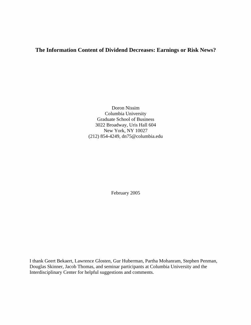
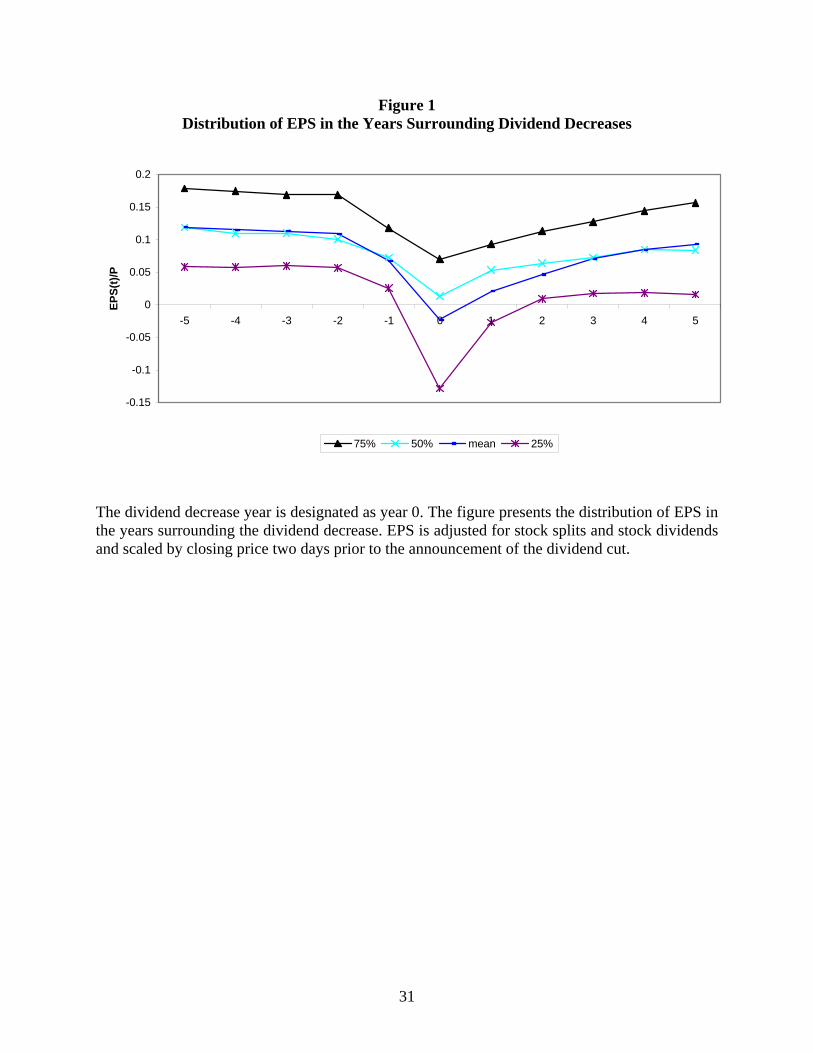
subsequent to the dividend cut.11 Figure 1 plots the distribution of EPS in each of the eleven

years surrounding the dividend decrease, scaled by closing price two days prior to the dividend

announcement (all per share data are adjusted for stock splits and stock dividends). The statistics

plotted are the 25th, 50th and 75th percentiles, and the mean. Panel A of Table 2 presents the mean

10 Qualitatively similar results are obtained without winsorizing, with trimming instead of winsorizing, and with alternative percentile cuts. 11 EPS is measured as COMPUSTAT’s data item #58 (basic earnings per share before extraordinary items and discontinued operations and adjusted for preferred dividends).

11

and median of earnings in the seven years surrounding the dividend decrease, as well as changes

in these quantities and the significance of the changes.12 As shown, current earnings (i.e.,

earnings in year 0) are considerably smaller than in the surrounding years, although the decrease

in earnings starts in year –1 (in years –5 through –2 earnings are relatively stable). Mean

earnings drops from 0.109 to 0.068 in year –1 (t-statistic for the change equals –7.5), and from

0.068 to –0.023 in year 0 (t-statistic for the change equals –10.7). From year 1 on, earnings

increase monotonically but at a slower pace than the rate of decline in year 0. Similar results are

obtained for median earnings, indicating that these trends are not due to outlier observations.

Consistent with the conjecture that firms are more likely to report negative special items

in dividend decrease years, the left tail of the earnings distribution flattens in year 0 (e.g., the

difference between the 50th and 25th percentiles in Figure 1 becomes substantially larger). The

flattening of the left tail is also reflected in the relationship between the mean and the median:

Mean earnings is similar to the median in years –5 through –1, but in year 0 the mean is

considerably smaller than the median. To verify the inference that firms report abnormal levels

of negative transitory items in dividend decrease years, I next examine the distribution of special

items.13

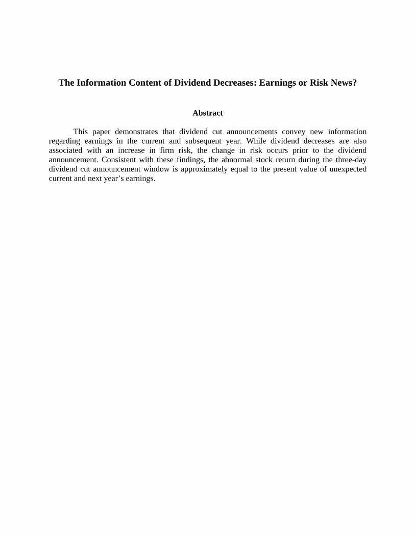
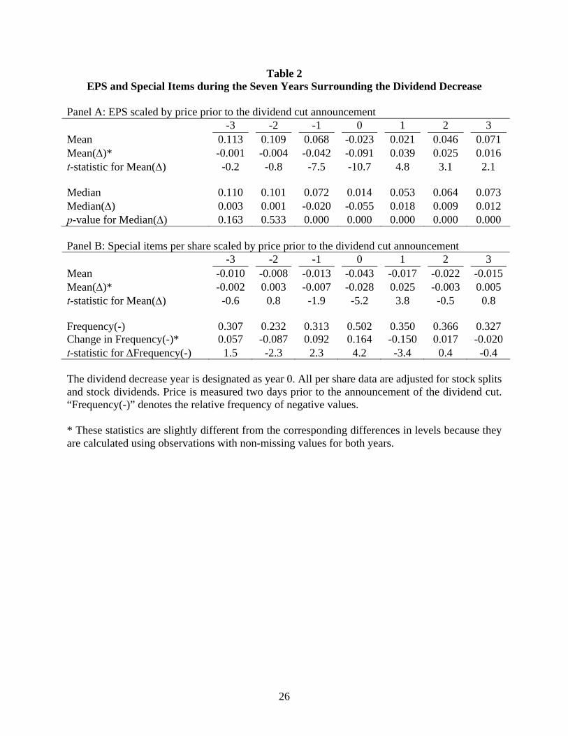
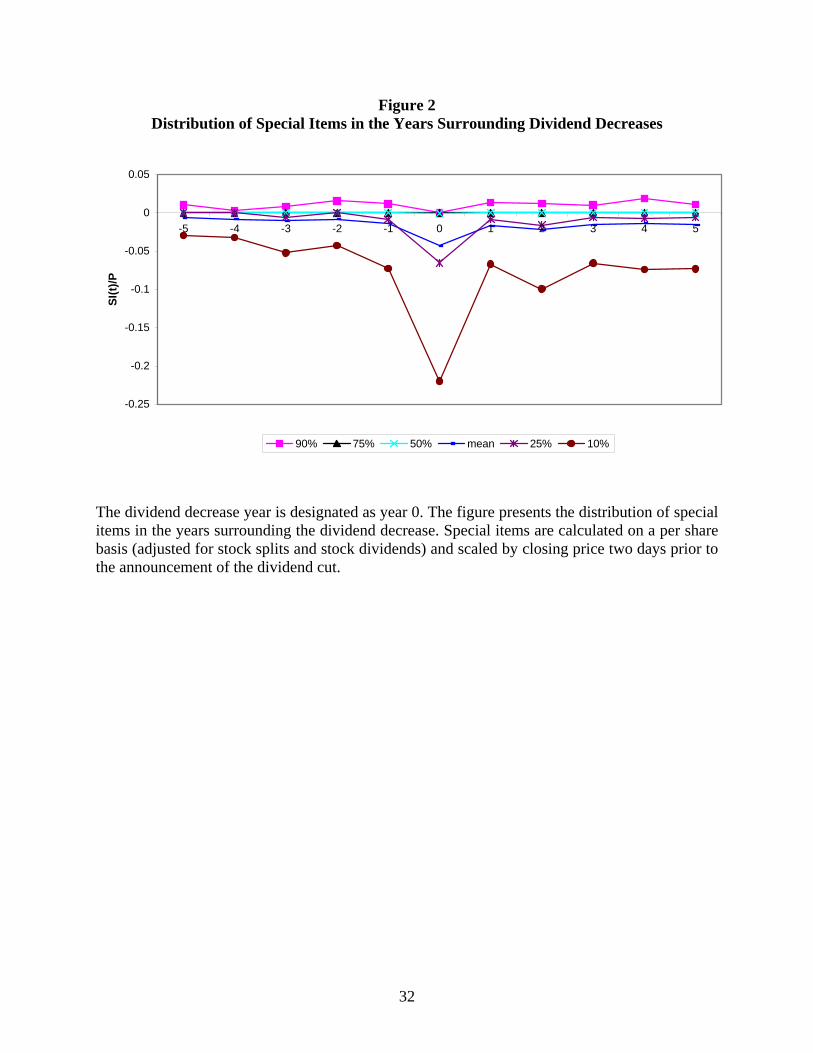
Figure 2 plots the cross-sectional distributions of special items per share in the years

surrounding the dividend cut, and Panel B of Table 2 presents summary and test statistics (mean,

frequency of negative values, changes in these statistics, and t-statistics for the changes). To hold

size constant, special items are scaled by closing price two days prior to the announcement of the 12 The change statistics are slightly different from the corresponding differences between the consecutive levels because they are calculated using observations with non-missing values for both years. 13 Special items are measured as COMPUSTAT’s data item #17. This item includes different types of revenues and expenses from continuing operations which are classified by firms as transitory (e.g., write-offs, impairments and restructuring charges). Special items are much more common and larger in magnitude than extraordinary items, which are rarely reported by companies. For a detailed discussion of special items, see Burgstahler et al. (2002).

12

dividend cut. Mean special items decreases from –0.013 in year –1 to –0.043 in year 0 (t-statistic

for the change equals –5.2) and increases back to –0.017 in year 1 (t-statistic equals 3.8). This

“V” shape pattern is especially apparent for the 10th percentile of the distribution (see Figure 2).

In addition, the frequency of negative special items increases from 31.3 percent in year –1 to

50.2 percent in year 0 (t-statistic for the change equals 4.2), and decreases back to 35.0 percent in

year 1 (t-statistic equals –3.4). After year 1, the frequency of negative special items remains

relatively stable.

To summarize, firms that cut their dividends report very low earnings in the year of the

dividend change, in large part due to the recognition of negative special items. Consistent with

the low persistence of special items (Burgstahler et al. (2002)), these firms report substantial EPS

increases in subsequent years. Yet, earnings reach their pre-dividend cut level only three years

after the dividend decrease. Although these results suggest that dividend decreases predict lower

current and future earnings, they do not indicate whether this information is revealed by the

dividend announcement rather than by prior disclosures such as interim earnings reports. I next

use market-based information to construct measures of expected earnings immediately prior to

the dividend change, which allow me to test whether dividend cut announcements convey new

earnings information.

B. Dividend Decreases and Unexpected Earnings

I start by examining the association between analysts’ forecast errors and dividend

changes. To the extent that analysts’ EPS forecasts reflect the market expectation of current and

future EPS, the average value of the forecast errors (i.e., the average difference between realized

and forecasted EPS) for dividend decrease firms should indicate whether dividend cuts convey

new earnings information to the market. Specifically, if the average value of analysts’ forecast

13

errors for dividend decrease firms is negative and significant, the inference would be that

dividend reductions convey negative earnings news.

This approach for testing the information content of dividends is straightforward

(analysts’ forecasts provide a direct measure of expected earnings) and simple to implement.

However, it has important shortcomings: Analysts’ forecasts are on average biased upward and

they do not reflect all available information (for a review of the literature documenting these

results, see Kothari 2001). I therefore compare the forecast errors of dividend cut firms with

those of other dividend paying firms rather than assume that the unconditional mean of the

forecast error is zero. In addition, I conduct multivariate analyses that mitigate the effect of

measurement error in the proxy for expected earnings by incorporating information from stock

prices and other variables in addition to analysts’ forecasts.

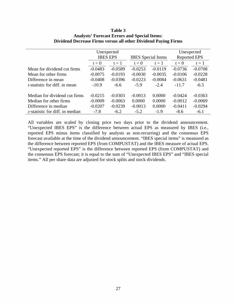
The results of the univariate analysis are reported in Table 3. This table presents the mean

and median analysts’ EPS forecast errors for dividend decrease firms and for all other dividend

paying firms. Analysts’ forecast errors (labeled “unexpected IBES EPS”) are measured as the

difference between the IBES measure of actual EPS and the consensus EPS forecast available at

the time of the dividend announcement. Actual EPS as measured by IBES is equal to reported

EPS minus items classified by analysts as non-recurring (“IBES special items”). The total

difference between reported and forecasted EPS (“unexpected reported EPS”) is equal to the sum

of “unexpected IBES EPS” and “IBES special items.”

Analysts’ forecast errors are negative for both dividend decrease firms and other dividend

paying firms, and are larger in magnitude in year 1 compared to year 0. Both results are

consistent with prior research, which demonstrates that analysts’ forecasts are biased upward

with the bias increasing in the forecast horizon. However, unexpected earnings are substantially

and significantly smaller for dividend decrease firms compared to other dividend paying firms.

14

Specifically, unexpected IBES earnings for dividend decrease firms are on average –4.83% of

price for year 0 and –5.89% for year 1, while the corresponding numbers for other dividend

paying firms are –0.75% and –1.93% respectively. These results are not due to outliers, as the

differences in median are also highly significant.

The magnitude of negative special items (middle two columns in Table 3) is substantially

larger for dividend decrease firms than for other dividend paying firms, especially in year 0 (–

2.53% of price for dividend decrease firms compared to –0.30% for other dividend paying

firms). These results are consistent with the statistics in Panel B of Table 2, which demonstrate

that firms report more negative special items in dividend decrease years than in other years.

Because special items are less persistent than other earnings items (e.g., Burgstahler et al.

(2002)), these findings imply that dividend decrease firms should experience earnings increases

in future years. Indeed, the results of prior research (e.g., Benartzi et al. (1997)) and this study

(Panel A of Table 2) indicate that dividend cuts are followed by earnings increases in subsequent

years. However, current earnings, the starting point of this earnings growth, are substantially

smaller than expected at the time of the dividend cut. Therefore, the level of future earnings may

still be lower than expected at the time of the dividend cut, in spite of the future earnings

increases. The statistics in Table 3 suggest that unexpected earnings in year t = 1 of dividend

decrease firms are indeed negative.

Thus far I have used analysts’ EPS forecasts to measure the market expectations of

current and future earnings. As discussed above, however, analysts’ forecasts contain error and

bias, which may be correlated with the characteristics of dividend decrease firms (e.g., small

size, low expected growth). Moreover, analysts’ forecasts may be stale, especially for dividend

decrease firms (given their small size and other less attractive characteristics). To mitigate these

effects, I next estimate regression model (5) which incorporates information from market prices

15

and other variables in addition to analysts’ forecasts. I start by replicating the results of prior

studies (e.g., Benartzi et al. (1997), Nissim and Ziv (2001)), which find that dividend reductions

are not associated with negative future earnings after controlling for current earnings. To this

end, I include in equation (5) the ratio of current earnings to price as an additional explanatory

variable.

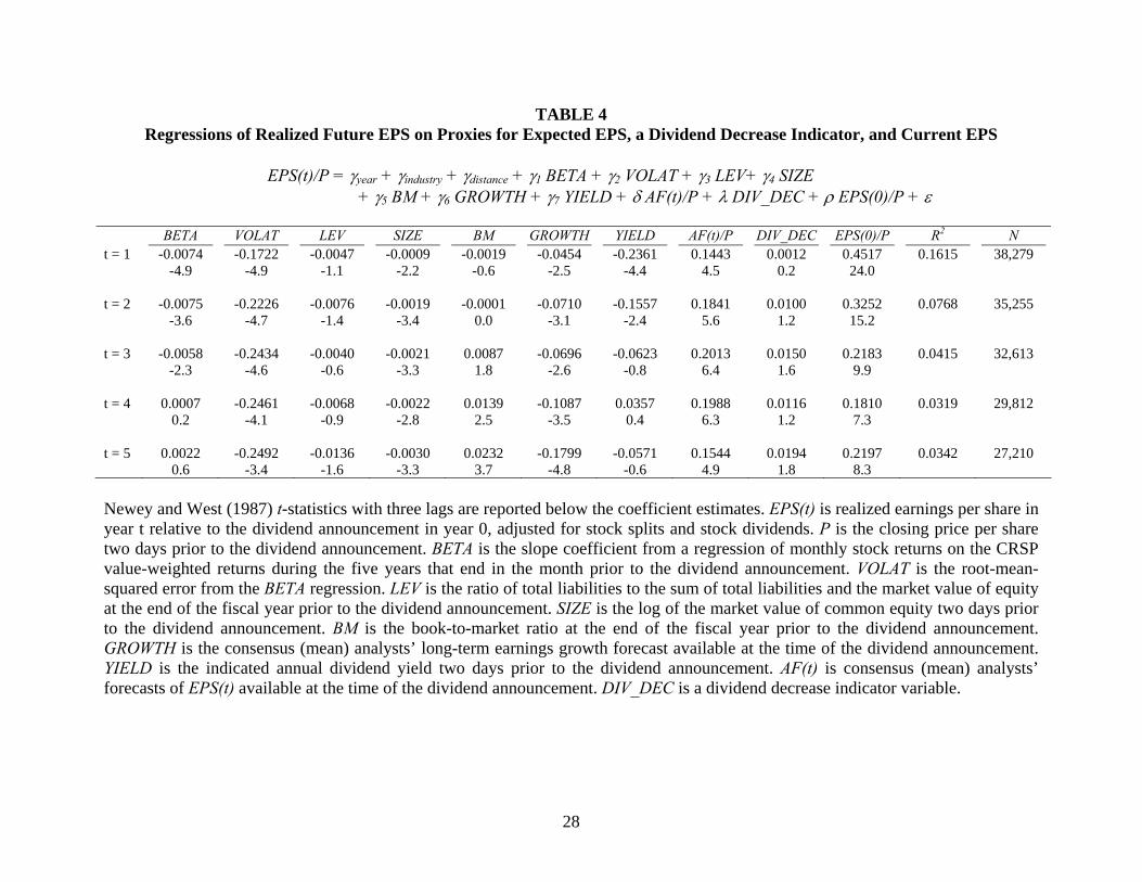
Table 4 presents the regression results. As shown, the coefficient of the dividend decrease

indicator variable (DIV_DEC) is non-negative in each of the five regressions (t = 1, 2, …, 5),

confirming that dividend decreases do not imply lower future earnings after controlling for

current earnings. But should one control for current earnings? As discussed above, if realized

current earnings of dividend decrease firms are smaller than expected at the time of the dividend

change, including them in the regression will bias the results against finding information content

in dividend decreases. The results in Tables 2 and 3 suggest that realized current earnings are

indeed smaller than expected at the time of the dividend change. Moreover, the high significance

of current earnings in explaining future earnings (Table 4), even after controlling for analysts’

forecasts, price and other earnings predictors, suggests that current earnings reflect information

about future earnings which is not available at the time of the dividend change.

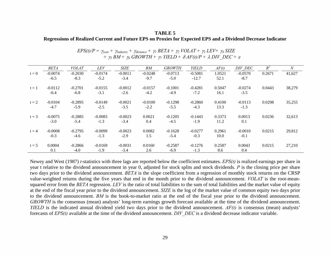
Miller and Rock (1985) predict the results of Table 4. They argue that dividend changes

convey information about future earnings indirectly by changing the market’s estimate of current

earnings, which in turn contributes to the estimate of future earnings. Thus, when current

earnings are included in the regression, the coefficient of the dividend change should be

insignificant, as I indeed find. In contrast, when the earnings expectation model reflects only

information which is available at the time of the dividend change, the coefficient of the dividend

change should be significant. I next examine this hypothesis by estimating equation (5), which

excludes current earnings. The estimates in Table 5 demonstrate that dividend decreases imply

16

lower current (t = 0) and next year (t = 1) earnings, but have no implications for earnings in later

years.

Assuming a discount rate between 10 to 20 percent, the dividend coefficients in Table 5

imply that dividend cut announcements should trigger negative stock returns between –7.8% (=

–0.0570/1.1.5 + –0.0274/1.11.5) and –7.3% (= –0.0570/1.2.5 + –0.0274/1.21.5). These estimates,

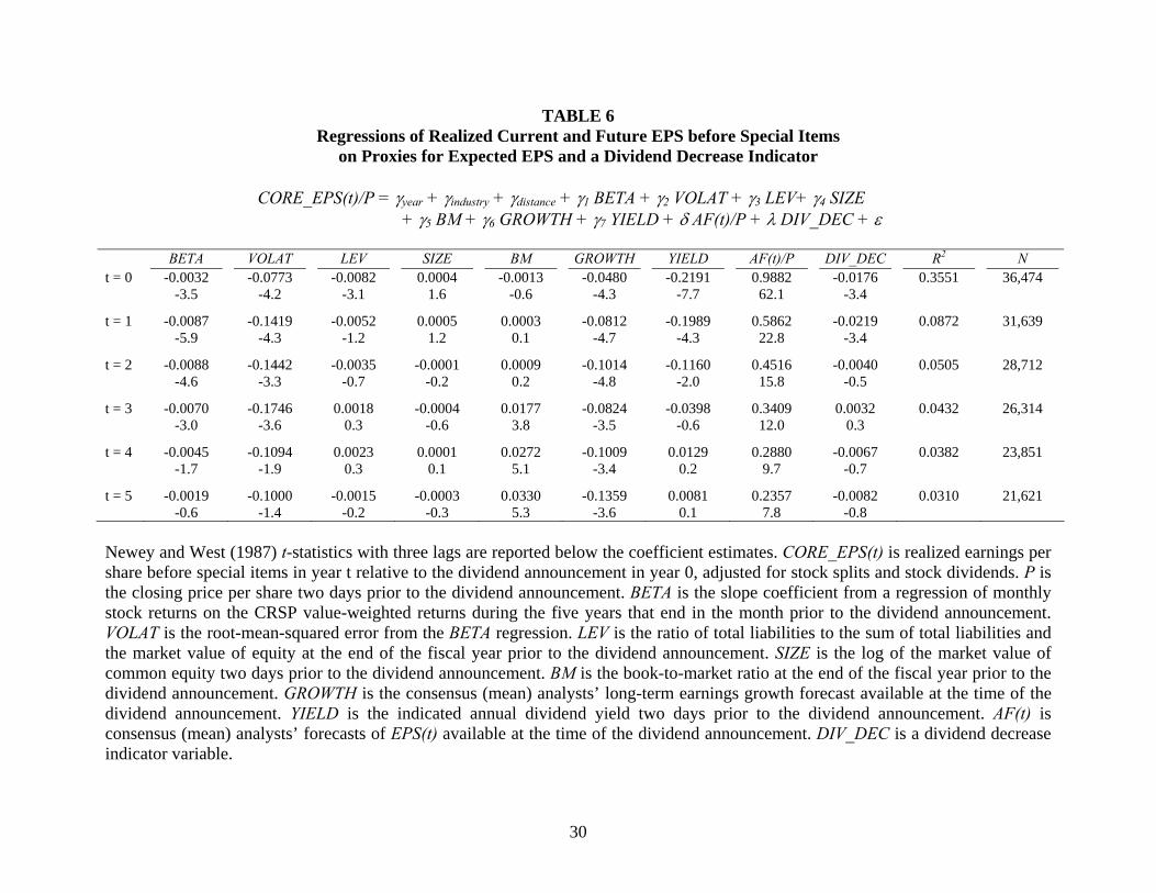
however, overstate the price impact of dividend cut announcements for two reasons. First, the

consensus analysts’ EPS forecast, which is the primary control variable, reflects analysts’

expectations of recurring earnings, while the dependent variable measures realized total earnings.

Thus, if dividend decrease firms are expected to report more negative special items than other

firms, the dividend decrease coefficient will be biased downward (it will capture expected

special items in addition to unexpected earnings and so overstate the negative implications of

dividend decreases). Second, negative special items which reduce reported earnings often reflect

“paper losses” with little cash flow consequences (e.g., impairment of goodwill). To address

these concerns, I next rerun equation (5) using CORE_EPS (EPS minus special items per share)

instead of reported EPS. The estimates in Table 6 suggest a substantially smaller value effect,

between –3.6% (= –0.0176/1.1.5 + –0.0219/1.11.5) and –3.3% (= –0.0176/1.2.5 + –0.0219/1.21.5),

assuming discount rate between 10 to 20 percent. Yet, similar to the results in Table 5, the

dividend coefficient is highly significant in both the t = 0 and t = 1 regressions.

C. Market Reaction to Dividend Cut Announcement

The estimates from the previous section suggest that dividend decrease announcements

should trigger an average stock decline of at least 3 percent, due to their negative earnings

implications. I next compare this estimate with the actual market response. I use the Fama and

French (FF, 1993) three-factor model to estimate the average abnormal stock return in each of

17

the 201 trading days centered at the dividend cut announcement. Specifically, for each relative

trading day (–100 through +100), I regress the following model using all firms that cut their

dividends in day 0:

teHMLγSMBγRMRFγγER ++++= 4321 , (6)

where ER is the daily excess stock return (raw return minus the risk-free return), RMRF is the

daily excess market return (market return minus the risk-free return), SMB is the daily return on a

portfolio long in small stocks and short in large stocks, and HML is the daily return on a portfolio

long in value stocks and short in growth stock.14 Under this approach, the intercept (γ1) of each

relative day regression measures the average abnormal stock return in that day for firms that

announce a dividend cut in day 0.

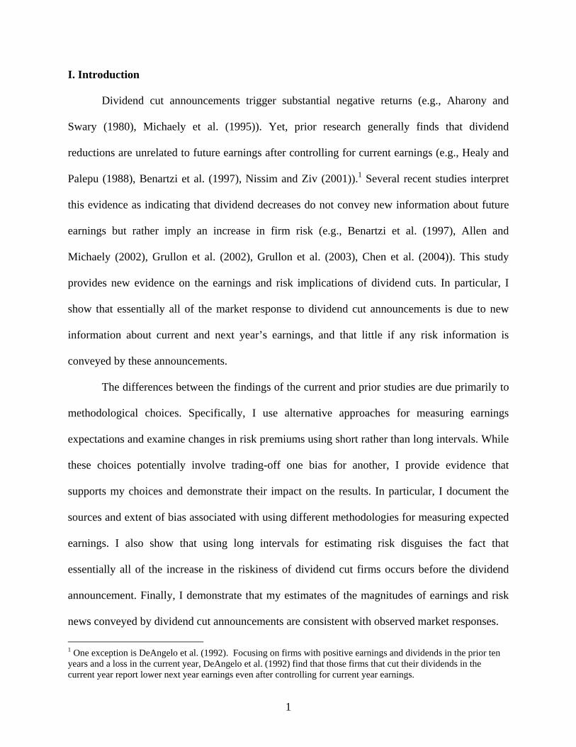
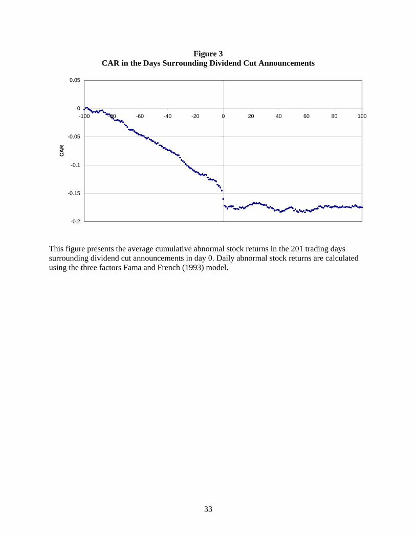
Figure 3 plots the cumulative average abnormal return for dividend decrease firms (i.e.,

the cumulative sum of the regression intercepts). Firms that cut their dividends in trading day 0

experience negative stock returns in the prior 100 trading days which sum up to a CAR of –14%

by the end of day –2. The three days announcement return (–1, 0, and 1) is equal to –3.2%, and it

is followed by a very slight drift in the following weeks. The overall market response is

approximately –3.5%, consistent with the estimates of the present value of unexpected earnings

reported in the previous subsection.15

14 Factor returns are obtained from WRDS. 15 The abnormal returns are slightly smaller than in prior studies (e.g., Aharony and Swary (1980)) due primarily to the requirement of availability of analysts’ forecasts (more recent sample period, larger firms). The small magnitude of the post announcement drift is consistent with the evidence in Grullon et al. (2002).

18

D. Dividend Decreases and Equity Risk

Grullon et al. (2002) find that dividend changes are associated with changes in equity

risk. In particular, they compare the FF factor loadings of dividend decrease firms in the three

years subsequent to the dividend change with the corresponding coefficients in the three prior

years and report significant increases in each of the three coefficients. They further estimate that

the annual risk premium increases by about 2% and argue that “changes in risk premium of this

magnitude are sufficient to generate the observed announcement-day price reactions” (page 388).

Indeed, changes of this magnitude should trigger very large negative returns if they are indicated

by the dividend announcement. In this section I examine the timeliness of the change in equity

risk.

I use the following procedure to examine changes over time in the risk premium of

dividend decrease firms. First, I calculate the average annualized return associated with each of

the three FF factors during the period July 1, 1963 through October 31, 2003.16 Second, I

estimate equation (6) for each of the relative trading days –1,250 through 1,250 for the sample of

dividend decrease firms. Third, I calculate the annualized risk premium associated with each

relative day using the factor loadings of equation (6) for that day and the average annualized

factor returns:

)()()(PremiumRisk Annualized 432 HMLAARγSMBAARγRMRFAARγ ++= (7)

where AAR(f) is the Average Annualized daily Return on factor f during 1963-2003, and γ2, γ3 and

γ4 are the estimated factor loadings for the particular trading day. Finally, I calculate the mean

16 The average annualized return on factor f is calculated as follows: AAR(f) = exp{252×mean[ln(1+f)]} – 1, where 252 is the average number of trading days per year and the mean is calculated over all daily observations during the period July 1, 1963 through October 31, 2003.

19

value of the annualized risk premium for groups of 50 consecutive trading days: (–1,250, –

1,201), (–1,200, –1,151), …, (–50, –1), (0, 49), …, (1,200, 1,249).

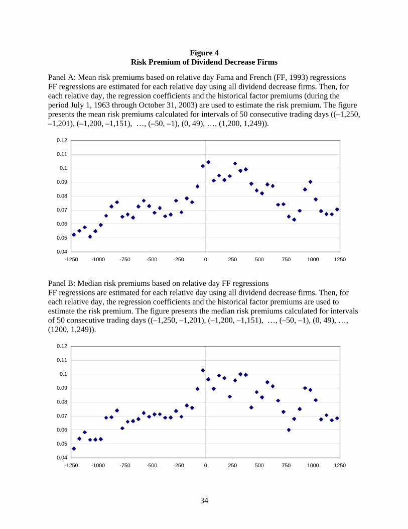
Panel A of Figure 4 plots the estimates. The x-axis displays the relative trading day while

the y-axis presents the mean value of the risk premium for each group of 50 consecutive trading

days. Consistent with Grullon et al. (2002), the average risk premium in the three years

subsequent to the dividend cut (trading days 0 through 750) is substantially larger than in the

prior three years. Specifically, the average risk premium in the three prior years is 7.4%

compared to 9.0% after the dividend cut (t-statistic for the difference equals 4.7). However, as is

evident from the figure, the increase in risk occurs gradually during the year preceding the

announcement of the dividend cut, and little if any additional increases occur after day –1. In

particular, during the intervals (–100, –51) and (–50, –1), the risk premium gradually increases

from less than 8% to more than 10%. It remains at this level for the next two years, and then

declines gradually to about 7%. This evidence suggests that dividend decreases follow rather

than signal increases in equity risk.

To examine the robustness of this result, I next use alternative approaches for calculating

the risk premium. First, I report the medians of the relative day risk premiums instead of the

means. The median estimates, plotted in Panel B of Figure 4, are very similar to the means

(Panel A). Second, instead of calculating means or medians for groups of consecutive trading

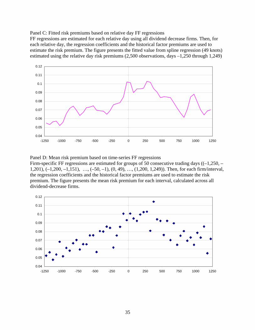
days, I fit a spline function with 49 knots (corresponding to 50 intervals) for the whole sample of

2,500 relative day risk premiums (days –1,250 through 1,249). Panel C of Figure 4 presents the

fitted value of the spline function. It is evident that all of the increase in the risk premium occurs

during the year preceding the announcement of the dividend cut.

The risk premium estimates in Panels A through C of Figure 4 are calculated by running

FF regressions for each relative trading day. Each regression includes all dividend decrease firms

20

with available stock returns for the particular relative day, and the estimates are based on the

assumption that all firms have the same factor loadings. The primary advantages of this approach

are that it allows the factor loadings to vary over relative time, and the factor loadings are

estimated using relatively large samples (up to 282 dividend decrease firms). Yet, dividend

decrease firms are not identical and may therefore have different factor loadings. To address this

concern, I rerun the analysis using time-series FF regressions. Specifically, for each firm, I

estimate time-series FF regressions for groups of 50 consecutive trading days ((–1,250, –1,201),

(–1,200, –1,151), …, (–50, –1), (0, 49), …, (1,200, 1,249)). I then calculate the firm/interval-

specific risk premium using the estimated factor loadings and the average annualized daily factor

returns over the period 1963-2003. Finally, for each interval, I calculate the mean and median

values of the risk premium across all firms. The resulting estimates are plotted in Panels D

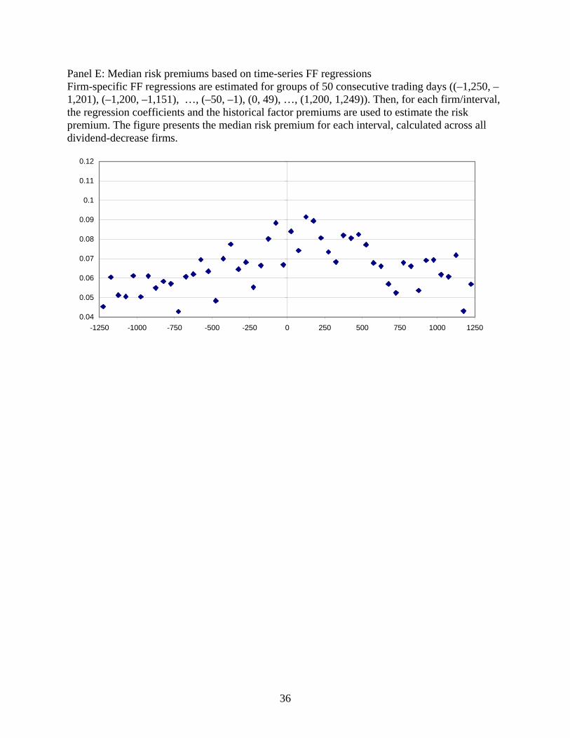
(means) and E (medians) of Figure 4.17

Consistent with the small number of observations per regression, the estimates in Panels

D and E of Figure 4 are more volatile than those in Panels A and B. Yet, in both Panels C and D,

the risk premium clearly increases prior to the dividend announcement and its average value in

the 150 trading days prior to the dividend change (the three points to the left of the y-axis) is

similar to the post-change values. Thus, the finding that dividend cut announcements follow

rather than signal an increase in risk is robust to the use of alternative approaches for measuring

risk premium.

17 To mitigate the impact of non-synchronous trading, I include in the FF regressions the one-day lag and lead values of each of the three factors and use the Scholes and Williams (1977) approach to adjust the estimated factor loadings.

21

E. Robustness Checks

I next conduct two robustness checks for the earnings analysis. First, I rerun all tests

involving analysts’ forecasts using the most recent analysts’ EPS and growth forecasts instead of

the respective consensus forecasts. I obtain qualitatively similar results to those reported above.

In particular, when regressing equation (5) with CORE_EPS as the dependent variable, I find

that the coefficient of the dividend decrease variable is –0.021 (t-statistic of –3.6) for year t = 0,

–0.029 (t-statistic of –4.4) for t = 1, and insignificant for t = 2, 3, 4, and 5. These estimates are

slightly larger in magnitude than those obtained with the consensus forecasts, suggesting that the

consensus forecasts are more precise than the most recent forecasts. The inference, however,

remains unchanged: Dividend cut announcements signal lower current and next year earnings.

Second, to evaluate the methodology, I estimate the regressions for large dividend

increases (greater than or equal to 20 percent) instead of dividend decreases.18 I find that the

dividend increase coefficient when explaining CORE_EPS is positive and significant for each of

the six years (t = 0, 1, …, 5), but its magnitude is relatively small (ranging between 0.007 and

0.013 with t-statistics ranging between 2.1 and 5.5). Thus, while both dividend decreases and

increases predict subsequent earnings, the information in dividend decreases relates primarily to

the near future while that in dividend increases is more permanent. This difference could be due

to accounting conservatism which requires that losses be recognized when anticipated while

profits should be recognized only when earned. Alternatively, the short duration of the negative

earnings implications of dividend cuts could be due to real options, such as the abandonment

option, which allow dividend decrease firms to improve or discontinue unsuccessful operations.

18 I focus on large dividend increases because, as shown in Table I, dividend decreases are substantially larger in magnitude than dividend increases.

22

VI. Conclusion

Extant research establishes that dividend decreases: (1) trigger negative stock returns, (2)

are unrelated to future earnings after controlling for current earnings, and (3) are associated with

an increase in firm risk. This evidence has been interpreted as suggesting that dividend cut

announcements signal an increase in risk, which in turn triggers a negative market response (e.g.,

Grullon et al. (2002)). I reexamine the information content of dividend decreases and find that

realized current earnings of dividend decrease firms contain negative special items and are

substantially smaller than expected at the time of the dividend change. These results imply that

controlling for current earnings in explaining future earnings biases the dividend coefficient

against finding information in dividend decreases.

I thus estimate an alternative model for expected earnings which extracts information

from analysts’ forecasts, price and other variables, but excludes current earnings. Using this

model, I find that dividend cut announcements are associated with negative unexpected earnings

in the subsequent year. I further show that the present value of unexpected earnings in the current

and next year is approximately equal to the dividend cut announcement return. Finally, I

demonstrate that the increase in the riskiness of dividend cut firms, which has been documented

by previous studies, occurs primarily in the year prior to the dividend announcement. I therefore

conclude that dividend decrease announcements convey earnings rather than risk information.

23

REFERENCES Aharony, Joseph, and Itzhak Swary, 1980, Quarterly dividend and earnings announcements and

stockholders’ returns: An empirical analysis, Journal of Finance 35, 1-12. Allen, Franklin, and Roni Michaely, 2002, Payout policy, Working paper, University of

Pennsylvania. Baker, Malcolm, and Richard S. Ruback, 1999, Estimating industry multiples, Working paper,

Harvard University. Beaver, William, and Dale Morse, 1978, What determines price-earnings ratios? Financial

Analysts Journal 34, 65-76. Benartzi, Shlomo, Roni Michaely, and Richard Thaler, 1997, Do changes in dividends signal the

future or the past? Journal of Finance 52, 1007-1034. Burgstahler, David, James Jiambalvo, and Terry Shevlin, 2002, Do stock prices fully reflect the

implications of special items for future earnings? Journal of Accounting Research 40, 585-612.

Chen, Shuping, Terry Shevlin, and Yen Hee Tong, 2004, What is the information content of

dividend changes? A new investigation of an old puzzle, Working paper, University of Washington.

DeAngelo, Harry, Linda DeAngelo, and Douglas J. Skinner, 1992, Dividends and losses, Journal

of Finance 47, 1837-1863. Elliott, John A., and Douglas J. Hanna, 1996, Repeated accounting write-offs and the

information content of earnings, Journal of Accounting Research 34, 135-155. Fairfield, Patricia M., 1994, P/E, P/B and the present value of future dividends, Financial

Analysts Journal 50, 23-31. Fama, Eugene F., and Kenneth R. French, 1993, Common risk factors in the returns on stocks

and bonds, Journal of Financial Economics 33, 3-56. Fama, Eugene F., and Kenneth R. French, 2001, Disappearing dividends: Changing firm

characteristics or lower propensity to pay, Journal of Financial Economics 60, 3-43. Gordon, Myron J., 1962, The Investment, Financing, and Valuation of the Corporation (Irwin,

Homewood, IL) Greenspan, Alan, 1997, Monetary Policy Report to Congress Pursuant to the Full Employment &

Balanced Growth Act of 1998, Superintendent of Documents.

24

Grullon, Gustavo, Roni Michaely, and Bhaskaran Swaminathan, 2002, Are dividend changes a sign of firm maturity? Journal of Business 75, 387-424.

Grullon, Gustavo, Shlomo Benartzi, Roni Michaely, and Richard H. Thaler, 2003, Dividend

changes do not signal changes in future profitability, Journal of Business (forthcoming). Healy, Paul M., and Krishna G. Palepu, 1988, Earnings information conveyed by dividend

initiations and omissions, Journal of Financial Economics 21, 149-175. Jacksonth, Scott B., and Marshall K. Pitman, 2001, Auditors and earnings management, The

CPA Journal 71, 38-44. Kirschenheiter, Michael, and Nahum Melumad, 2001, Can “big bath” and earnings smoothing

co-exist as equilibrium financial reporting strategies? Journal of Accounting Research 40, 761-96.

Kothari, S.P., 2001, Capital markets research in accounting, Journal of Accounting and

Economics 31, 105-231. Michaely, Roni, Richard H. Thaler, and Kent L. Womack, 1995, Price reactions to dividend

initiations and omissions: Overreaction or drift? Journal of Finance 50, 573-608. Miller, Merton H., and Kevin Rock, 1985, Dividend policy under asymmetric information,

Journal of Finance 40, 1031-1051. Newey, Whitney K., and Kenneth D. West, 1987, A simple positive semi-definite,

heteroskedasticity and autocorrelation consistent covariance matrix, Econometrica 55, 703-708.

Nissim, Doron, and Amir Ziv, 2001, Dividend changes and future profitability, Journal of

Finance 56, 2111-2134. Scholes, Myron, and Joseph Williams, 1977, Estimating beta from non-synchronous data,

Journal of Financial Economics 5, 309-327. Skinner, Douglas J., 2003, What do dividends tell us about earnings quality? Working paper,

University of Michigan. Zarowin, Paul, 1990, What determines earnings–price ratios: Revisited, Journal of Accounting,

Auditing & Finance 5, 439-457.

25

Table 1 Descriptive Statistics

Dividend Decrease

(N = 282) No change

(N = 35,769) Dividend Increase

(N = 5,576) Mean Med. StD Mean Med. StD Mean Med. StD R∆DIV -0.456 -0.500 0.239 0.000 0.000 0.000 0.129 0.098 0.203 BETA 0.830 0.815 0.458 0.915 0.915 0.440 0.868 0.874 0.434 VOLAT 0.081 0.078 0.025 0.076 0.073 0.025 0.071 0.067 0.023 LEV 0.561 0.595 0.248 0.501 0.496 0.249 0.521 0.510 0.275 SIZE 6.431 6.510 1.631 6.781 6.715 1.585 6.985 6.921 1.548 BM 0.829 0.752 0.420 0.623 0.580 0.321 0.568 0.548 0.274 GROWTH 0.095 0.090 0.048 0.117 0.116 0.044 0.114 0.115 0.042 YIELD 0.064 0.064 0.028 0.031 0.026 0.020 0.030 0.025 0.019 R∆DIV is the rate of change in quarterly dividend per share. BETA is the slope coefficient from a regression of monthly stock returns on the CRSP value-weighted returns during the five years that end in the month prior to the dividend announcement. VOLAT is the root-mean-squared error from the BETA regression. LEV is the ratio of total liabilities to the sum of total liabilities and the market value of equity at the end of the fiscal year prior to the dividend announcement. SIZE is the log of the market value of common equity two days prior to the dividend announcement. BM is the book-to-market ratio at the end of the fiscal year prior to the dividend announcement. GROWTH is the consensus (mean) analysts’ long-term earnings growth forecast available at the time of the dividend announcement. YIELD is the indicated annual dividend yield two days prior to the dividend announcement.

26

Table 2 EPS and Special Items during the Seven Years Surrounding the Dividend Decrease

Panel A: EPS scaled by price prior to the dividend cut announcement -3 -2 -1 0 1 2 3 Mean 0.113 0.109 0.068 -0.023 0.021 0.046 0.071 Mean(∆)* -0.001 -0.004 -0.042 -0.091 0.039 0.025 0.016 t-statistic for Mean(∆) -0.2 -0.8 -7.5 -10.7 4.8 3.1 2.1 Median 0.110 0.101 0.072 0.014 0.053 0.064 0.073 Median(∆) 0.003 0.001 -0.020 -0.055 0.018 0.009 0.012 p-value for Median(∆) 0.163 0.533 0.000 0.000 0.000 0.000 0.000 Panel B: Special items per share scaled by price prior to the dividend cut announcement -3 -2 -1 0 1 2 3 Mean -0.010 -0.008 -0.013 -0.043 -0.017 -0.022 -0.015 Mean(∆)* -0.002 0.003 -0.007 -0.028 0.025 -0.003 0.005 t-statistic for Mean(∆) -0.6 0.8 -1.9 -5.2 3.8 -0.5 0.8 Frequency(-) 0.307 0.232 0.313 0.502 0.350 0.366 0.327 Change in Frequency(-)* 0.057 -0.087 0.092 0.164 -0.150 0.017 -0.020 t-statistic for ∆Frequency(-) 1.5 -2.3 2.3 4.2 -3.4 0.4 -0.4 The dividend decrease year is designated as year 0. All per share data are adjusted for stock splits and stock dividends. Price is measured two days prior to the announcement of the dividend cut. “Frequency(-)” denotes the relative frequency of negative values. * These statistics are slightly different from the corresponding differences in levels because they are calculated using observations with non-missing values for both years.

27

Table 3 Analysts’ Forecast Errors and Special Items:

Dividend Decrease Firms versus all other Dividend Paying Firms Unexpected

IBES EPS

IBES Special Items Unexpected

Reported EPS t = 0 t = 1 t = 0 t = 1 t = 0 t = 1 Mean for dividend cut firms -0.0483 -0.0589 -0.0253 -0.0119 -0.0736 -0.0708 Mean for other firms -0.0075 -0.0193 -0.0030 -0.0035 -0.0106 -0.0228 Difference in mean -0.0408 -0.0396 -0.0223 -0.0084 -0.0631 -0.0481 t-statistic for diff. in mean -10.9 -6.6 -5.9 -2.4 -11.7 -6.5 Median for dividend cut firms -0.0215 -0.0303 -0.0013 0.0000 -0.0424 -0.0363 Median for other firms -0.0009 -0.0063 0.0000 0.0000 -0.0012 -0.0069 Difference in median -0.0207 -0.0239 -0.0013 0.0000 -0.0411 -0.0294 z-statistic for diff. in median -7.8 -6.2 -5.2 -1.9 -8.6 -6.1 All variables are scaled by closing price two days prior to the dividend announcement. “Unexpected IBES EPS” is the difference between actual EPS as measured by IBES (i.e., reported EPS minus items classified by analysts as non-recurring) and the consensus EPS forecast available at the time of the dividend announcement. “IBES special items” is measured as the difference between reported EPS (from COMPUSTAT) and the IBES measure of actual EPS. “Unexpected reported EPS” is the difference between reported EPS (from COMPUSTAT) and the consensus EPS forecast; it is equal to the sum of “Unexpected IBES EPS” and “IBES special items.” All per share data are adjusted for stock splits and stock dividends.

28

TABLE 4 Regressions of Realized Future EPS on Proxies for Expected EPS, a Dividend Decrease Indicator, and Current EPS

EPS(t)/P = γyear + γindustry + γdistance + γ1 BETA + γ2 VOLAT + γ3 LEV+ γ4 SIZE + γ5 BM + γ6 GROWTH + γ7 YIELD + δ AF(t)/P + λ DIV_DEC + ρ EPS(0)/P + ε BETA VOLAT LEV SIZE BM GROWTH YIELD AF(t)/P DIV_DEC EPS(0)/P R2 N t = 1 -0.0074 -0.1722 -0.0047 -0.0009 -0.0019 -0.0454 -0.2361 0.1443 0.0012 0.4517 0.1615 38,279

-4.9 -4.9 -1.1 -2.2 -0.6 -2.5 -4.4 4.5 0.2 24.0

t = 2 -0.0075 -0.2226 -0.0076 -0.0019 -0.0001 -0.0710 -0.1557 0.1841 0.0100 0.3252 0.0768 35,255

-3.6 -4.7 -1.4 -3.4 0.0 -3.1 -2.4 5.6 1.2 15.2

t = 3 -0.0058 -0.2434 -0.0040 -0.0021 0.0087 -0.0696 -0.0623 0.2013 0.0150 0.2183 0.0415 32,613

-2.3 -4.6 -0.6 -3.3 1.8 -2.6 -0.8 6.4 1.6 9.9

t = 4 0.0007 -0.2461 -0.0068 -0.0022 0.0139 -0.1087 0.0357 0.1988 0.0116 0.1810 0.0319 29,812

0.2 -4.1 -0.9 -2.8 2.5 -3.5 0.4 6.3 1.2 7.3

t = 5 0.0022 -0.2492 -0.0136 -0.0030 0.0232 -0.1799 -0.0571 0.1544 0.0194 0.2197 0.0342 27,210 0.6 -3.4 -1.6 -3.3 3.7 -4.8 -0.6 4.9 1.8 8.3 Newey and West (1987) t-statistics with three lags are reported below the coefficient estimates. EPS(t) is realized earnings per share in year t relative to the dividend announcement in year 0, adjusted for stock splits and stock dividends. P is the closing price per share two days prior to the dividend announcement. BETA is the slope coefficient from a regression of monthly stock returns on the CRSP value-weighted returns during the five years that end in the month prior to the dividend announcement. VOLAT is the root-mean-squared error from the BETA regression. LEV is the ratio of total liabilities to the sum of total liabilities and the market value of equity at the end of the fiscal year prior to the dividend announcement. SIZE is the log of the market value of common equity two days prior to the dividend announcement. BM is the book-to-market ratio at the end of the fiscal year prior to the dividend announcement. GROWTH is the consensus (mean) analysts’ long-term earnings growth forecast available at the time of the dividend announcement. YIELD is the indicated annual dividend yield two days prior to the dividend announcement. AF(t) is consensus (mean) analysts’ forecasts of EPS(t) available at the time of the dividend announcement. DIV_DEC is a dividend decrease indicator variable.

29

TABLE 5 Regressions of Realized Current and Future EPS on Proxies for Expected EPS and a Dividend Decrease Indicator

EPS(t)/P = γyear + γindustry + γdistance + γ1 BETA + γ2 VOLAT + γ3 LEV+ γ4 SIZE + γ5 BM + γ6 GROWTH + γ7 YIELD + δ AF(t)/P + λ DIV_DEC + ε BETA VOLAT LEV SIZE BM GROWTH YIELD AF(t) DIV_DEC R2 N t = 0 -0.0074 -0.2030 -0.0174 -0.0011 -0.0248 -0.0713 -0.5081 1.0521 -0.0570 0.2671 41,627

-6.5 -8.3 -5.2 -3.4 -9.7 -5.0 -12.7 52.1 -8.7

t = 1 -0.0112 -0.2701 -0.0155 -0.0012 -0.0157 -0.1001 -0.4281 0.5047 -0.0274 0.0443 38,279

-6.4 -6.8 -3.1 -2.6 -4.2 -4.9 -7.2 16.1 -3.5

t = 2 -0.0104 -0.2895 -0.0149 -0.0021 -0.0100 -0.1298 -0.2860 0.4100 -0.0113 0.0298 35,255

-4.7 -5.9 -2.5 -3.5 -2.2 -5.5 -4.3 13.3 -1.3

t = 3 -0.0075 -0.2885 -0.0083 -0.0023 0.0021 -0.1205 -0.1443 0.3373 0.0013 0.0236 32,613

-3.0 -5.4 -1.3 -3.4 0.4 -4.5 -1.9 11.2 0.1

t = 4 -0.0008 -0.2795 -0.0099 -0.0023 0.0082 -0.1628 -0.0277 0.2961 -0.0010 0.0215 29,812

-0.3 -4.6 -1.3 -2.9 1.5 -5.4 -0.3 10.0 -0.1

t = 5 0.0004 -0.2866 -0.0169 -0.0031 0.0160 -0.2587 -0.1276 0.2587 0.0043 0.0215 27,210 0.1 -4.0 -1.9 -3.4 2.6 -6.9 -1.3 8.6 0.4 Newey and West (1987) t-statistics with three lags are reported below the coefficient estimates. EPS(t) is realized earnings per share in year t relative to the dividend announcement in year 0, adjusted for stock splits and stock dividends. P is the closing price per share two days prior to the dividend announcement. BETA is the slope coefficient from a regression of monthly stock returns on the CRSP value-weighted returns during the five years that end in the month prior to the dividend announcement. VOLAT is the root-mean-squared error from the BETA regression. LEV is the ratio of total liabilities to the sum of total liabilities and the market value of equity at the end of the fiscal year prior to the dividend announcement. SIZE is the log of the market value of common equity two days prior to the dividend announcement. BM is the book-to-market ratio at the end of the fiscal year prior to the dividend announcement. GROWTH is the consensus (mean) analysts’ long-term earnings growth forecast available at the time of the dividend announcement. YIELD is the indicated annual dividend yield two days prior to the dividend announcement. AF(t) is consensus (mean) analysts’ forecasts of EPS(t) available at the time of the dividend announcement. DIV_DEC is a dividend decrease indicator variable.

30

TABLE 6 Regressions of Realized Current and Future EPS before Special Items

on Proxies for Expected EPS and a Dividend Decrease Indicator CORE_EPS(t)/P = γyear + γindustry + γdistance + γ1 BETA + γ2 VOLAT + γ3 LEV+ γ4 SIZE + γ5 BM + γ6 GROWTH + γ7 YIELD + δ AF(t)/P + λ DIV_DEC + ε BETA VOLAT LEV SIZE BM GROWTH YIELD AF(t)/P DIV_DEC R2 N t = 0 -0.0032 -0.0773 -0.0082 0.0004 -0.0013 -0.0480 -0.2191 0.9882 -0.0176 0.3551 36,474

-3.5 -4.2 -3.1 1.6 -0.6 -4.3 -7.7 62.1 -3.4

t = 1 -0.0087 -0.1419 -0.0052 0.0005 0.0003 -0.0812 -0.1989 0.5862 -0.0219 0.0872 31,639

-5.9 -4.3 -1.2 1.2 0.1 -4.7 -4.3 22.8 -3.4

t = 2 -0.0088 -0.1442 -0.0035 -0.0001 0.0009 -0.1014 -0.1160 0.4516 -0.0040 0.0505 28,712

-4.6 -3.3 -0.7 -0.2 0.2 -4.8 -2.0 15.8 -0.5

t = 3 -0.0070 -0.1746 0.0018 -0.0004 0.0177 -0.0824 -0.0398 0.3409 0.0032 0.0432 26,314

-3.0 -3.6 0.3 -0.6 3.8 -3.5 -0.6 12.0 0.3

t = 4 -0.0045 -0.1094 0.0023 0.0001 0.0272 -0.1009 0.0129 0.2880 -0.0067 0.0382 23,851

-1.7 -1.9 0.3 0.1 5.1 -3.4 0.2 9.7 -0.7

t = 5 -0.0019 -0.1000 -0.0015 -0.0003 0.0330 -0.1359 0.0081 0.2357 -0.0082 0.0310 21,621 -0.6 -1.4 -0.2 -0.3 5.3 -3.6 0.1 7.8 -0.8

Newey and West (1987) t-statistics with three lags are reported below the coefficient estimates. CORE_EPS(t) is realized earnings per share before special items in year t relative to the dividend announcement in year 0, adjusted for stock splits and stock dividends. P is the closing price per share two days prior to the dividend announcement. BETA is the slope coefficient from a regression of monthly stock returns on the CRSP value-weighted returns during the five years that end in the month prior to the dividend announcement. VOLAT is the root-mean-squared error from the BETA regression. LEV is the ratio of total liabilities to the sum of total liabilities and the market value of equity at the end of the fiscal year prior to the dividend announcement. SIZE is the log of the market value of common equity two days prior to the dividend announcement. BM is the book-to-market ratio at the end of the fiscal year prior to the dividend announcement. GROWTH is the consensus (mean) analysts’ long-term earnings growth forecast available at the time of the dividend announcement. YIELD is the indicated annual dividend yield two days prior to the dividend announcement. AF(t) is consensus (mean) analysts’ forecasts of EPS(t) available at the time of the dividend announcement. DIV_DEC is a dividend decrease indicator variable.

31

Figure 1 Distribution of EPS in the Years Surrounding Dividend Decreases

-0.15

-0.1

-0.05

0

0.05

0.1

0.15

0.2

-5 -4 -3 -2 -1 0 1 2 3 4 5

EPS(

t)/P

75% 50% mean 25%

The dividend decrease year is designated as year 0. The figure presents the distribution of EPS in the years surrounding the dividend decrease. EPS is adjusted for stock splits and stock dividends and scaled by closing price two days prior to the announcement of the dividend cut.

32

Figure 2 Distribution of Special Items in the Years Surrounding Dividend Decreases

-0.25

-0.2

-0.15

-0.1

-0.05

0

0.05

-5 -4 -3 -2 -1 0 1 2 3 4 5

SI(t)

/P

90% 75% 50% mean 25% 10%

The dividend decrease year is designated as year 0. The figure presents the distribution of special items in the years surrounding the dividend decrease. Special items are calculated on a per share basis (adjusted for stock splits and stock dividends) and scaled by closing price two days prior to the announcement of the dividend cut.

33

Figure 3 CAR in the Days Surrounding Dividend Cut Announcements

-0.2

-0.15

-0.1

-0.05

0

0.05

-100 -80 -60 -40 -20 0 20 40 60 80 100

CA

R

This figure presents the average cumulative abnormal stock returns in the 201 trading days surrounding dividend cut announcements in day 0. Daily abnormal stock returns are calculated using the three factors Fama and French (1993) model.

34

Figure 4 Risk Premium of Dividend Decrease Firms

Panel A: Mean risk premiums based on relative day Fama and French (FF, 1993) regressions FF regressions are estimated for each relative day using all dividend decrease firms. Then, for each relative day, the regression coefficients and the historical factor premiums (during the period July 1, 1963 through October 31, 2003) are used to estimate the risk premium. The figure presents the mean risk premiums calculated for intervals of 50 consecutive trading days ((–1,250, –1,201), (–1,200, –1,151), …, (–50, –1), (0, 49), …, (1,200, 1,249)).

0.04

0.05

0.06

0.07

0.08

0.09

0.1

0.11

0.12

-1250 -1000 -750 -500 -250 0 250 500 750 1000 1250

Panel B: Median risk premiums based on relative day FF regressions FF regressions are estimated for each relative day using all dividend decrease firms. Then, for each relative day, the regression coefficients and the historical factor premiums are used to estimate the risk premium. The figure presents the median risk premiums calculated for intervals of 50 consecutive trading days ((–1,250, –1,201), (–1,200, –1,151), …, (–50, –1), (0, 49), …, (1200, 1,249)).

0.04

0.05

0.06

0.07

0.08

0.09

0.1

0.11

0.12

-1250 -1000 -750 -500 -250 0 250 500 750 1000 1250

35

Panel C: Fitted risk premiums based on relative day FF regressions FF regressions are estimated for each relative day using all dividend decrease firms. Then, for each relative day, the regression coefficients and the historical factor premiums are used to estimate the risk premium. The figure presents the fitted value from spline regression (49 knots) estimated using the relative day risk premiums (2,500 observations, days –1,250 through 1,249)

0.04

0.05

0.06

0.07

0.08

0.09

0.1

0.11

0.12

-1250 -1000 -750 -500 -250 0 250 500 750 1000 1250

Panel D: Mean risk premium based on time-series FF regressions Firm-specific FF regressions are estimated for groups of 50 consecutive trading days ((–1,250, –1,201), (–1,200, –1,151), …, (–50, –1), (0, 49), …, (1,200, 1,249)). Then, for each firm/interval, the regression coefficients and the historical factor premiums are used to estimate the risk premium. The figure presents the mean risk premium for each interval, calculated across all dividend-decrease firms.

0.04

0.05

0.06

0.07

0.08

0.09

0.1

0.11

0.12

-1250 -1000 -750 -500 -250 0 250 500 750 1000 1250

36

Panel E: Median risk premiums based on time-series FF regressions Firm-specific FF regressions are estimated for groups of 50 consecutive trading days ((–1,250, –1,201), (–1,200, –1,151), …, (–50, –1), (0, 49), …, (1,200, 1,249)). Then, for each firm/interval, the regression coefficients and the historical factor premiums are used to estimate the risk premium. The figure presents the median risk premium for each interval, calculated across all dividend-decrease firms.

0.04

0.05

0.06

0.07

0.08

0.09

0.1

0.11

0.12

-1250 -1000 -750 -500 -250 0 250 500 750 1000 1250