The information content of short selling and put option

Tasmanian School of Business and Economics University of Tasmania

Discussion Paper Series N 2017-13

The information content of short selling and put option trading: When are they

substitutes?

Xiaohu Deng

University of Tasmania, Australia

Lei Gao

Iowa State University, USA

David M. Kemme

The University of Memphis, USA

ISBN 978-1-925646-05-04

1

The information content of short selling and put option trading: When

are they substitutes?*

This Draft: August, 2017

Abstract

Using January 2005 – June 2007 trading data for all NYSE stocks we identify the

informational patterns and impact of exogenous shocks in short sales and option trades

upon stock price changes. We find that short sales have more predictive power than put

option trades. However, if short selling volume is low put options trading does have

predictive power and thus may be a substitute used by informed investors.

Key words: Short selling; Put option trades; Informational patterns; Price discovery

JEL Codes: G12; G14

2

The information content of short selling and put option trading: When

are they substitutes?*

Xiaohu Deng

Tasmanian School of Business and Economics

The University of Tasmania

Hobart, TAS 7001, Australia

[email protected]

Lei Gao

Department of Finance

Iowa State University

Ames, IA 50011, USA

[email protected]

David M. Kemme

Department of Economics

The University of Memphis

Memphis, TN 38152, USA

[email protected]

* We would like to thank Alex Kurov, Lucjan Orlowski, Jacob Kleinow, Thomas Poppe,

and seminar participants at the University of Memphis, Midwest Finance Association

2015 Annual Meeting, and Financial Management Association 2015 Annual Meeting for

helpful comments. All mistakes and errors remain ours.

mailto:[email protected]



3

1. Introduction

Two major venues that mostly informed investors use, short sales and put options

trading, are both found to contain privileged and negative information (e.g. Chakravarty,

Gulen, and Mayhew, 2004; Cao, Chen, and Griffin, 2005; Diether, Lee, and Werner,

2009; Hao, Lee, and Piqueira, 2013; and etc). Nevertheless, whether short sellers and put

option traders are equally informed is not clear. Further, whether or not informed trading

in short sales and put option trades are essentially substitutes is also an open question. We

provide answers to these questions.

Early theory (Black, 1975; Easley, O’Hara, and Srinivas, 1998) suggested that

informed traders participate in both option and short equity markets. Subsequent

empirical studies supported to varying degrees the presence of informed trading in both

markets, which then in turn may be revealed in the equity market. However, the evidence

regarding which market is the primary venue for the most informed traders is still mixed.

Anthony (1988) analyzed the relationship between option and stock markets and shows

that call option trading volume predicts trading in the stock market on the next day. But

Chan, Chung, and Fong (2002) found that informed investors prefer to trade directly in

the stock market. Studies directly comparing the informativeness of option traders and

short sellers are few.

Short sales are driven by public and private information. However, put option

trades can be driven not only by information but also by liquidity shocks and hedging

needs (Chesney, Crameri, and Mancini, 2015). For this reason, we expect that a number

of short sales and put option trades are not made by the same group of investors.

Compared to put options trades, short sales, in turn, should contain different information

4

content. Moreover, as short sales are mostly information driven, and put options trades

are driven by different reasons, we conjecture that short selling contains more

information, i.e. predictive power, than put option trades, i.e. causality flows form short

selling to put option trading and stock price changes. We find this to be true in general,

but under certain circumstances put option trading has more predictive power. We

quantify the contribution to price discovery for these two groups of informed investors.

Using January 2005 – June 2007 trading data for all NYSE stocks, we determine

the information precedence of short sales and put option trading. We extend Hasbrouck’s

(1991) bivariate VAR model of stock market trades to also include put option trades and

short sales, and determine the optimal model by lag length tests on the independent

variables, and Wald tests of the vector of coefficients of each independent variable rather

than t-tests of individual coefficients. This approach confirms Granger causality tests and

combined, determines the direction of information flows, or predictability. Then, with

these orderings we specify a Choleski decomposition which allows us to identify the

VAR and calculate impulse response functions (IRFs). These responses to shocks in short

sales and put option trades and their persistence in each market allow us to compare the

informational patterns of short sales and put option trades. We repeat this for subsamples

based on short and put option trading intensity.

In general, the VAR results suggest short sales can predict future stock returns, yet

options cannot. This is consistent with the recent finding that option trades do not contain

as much information as short sales (see, Hao, Lee, and Piqueira, 2013; Muravyev,

Pearson, and Broussard, 2013). The impulse response functions indicate that stock prices

respond negatively to a shock in short sales for one to two days, and do not exhibit any

5

statistically significant response to the shock in put option trades. This then suggests that

short sales contain information that takes longer to incorporate into stock prices than put

option trading.

According to our finding and the empirical evidence from the recent literature (e.g.

Hao, Lee, and Piqueira, 2013), short sales contain more information. However, the

literature suggests put options can be informed under some circumstances, such as when

selling stock is expensive or there are some other restrictions to sell stocks short1. To test

whether market conditions influence whether put options and short sales can be

substitutes, we analyze several subsamples. We partition our sample by volume of short

sales and put option trades, re-estimate the VAR and IRFs. For heavily-shorted stocks,

short sales always have predictive power for future stock returns. However, we do not

find that put option trades of also heavily-shorted stocks has any significant predictive

power for future stock returns, regardless of the amount of put options traded on the same

underlying stocks. However, an important finding is that for lightly-shorted stocks, put

option trades show predictive power for future stock returns. This can be due to short

sales constraints so that most of informed traders reroute to put option trading venue

(Figlewski and Webb, 1993). This finding holds only when put option trading is intensive

and short selling is not.

The impulse responses further confirm that short sales contain more information.

The impulse responses for subsamples show the similar subsample variations. For

heavily-shorted stocks, stock returns to the shock in short sales exhibit a negative

1 Non-comprehensive list includes Figlewski and Webb (1993), Danielsen and Sorescu (2001), and Blau

and Wade (2011).

6

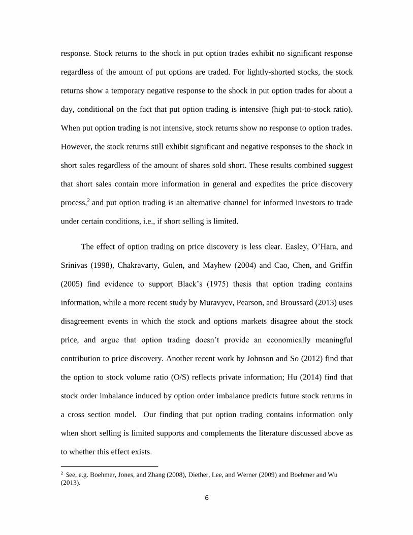
response. Stock returns to the shock in put option trades exhibit no significant response

regardless of the amount of put options are traded. For lightly-shorted stocks, the stock

returns show a temporary negative response to the shock in put option trades for about a

day, conditional on the fact that put option trading is intensive (high put-to-stock ratio).

When put option trading is not intensive, stock returns show no response to option trades.

However, the stock returns still exhibit significant and negative responses to the shock in

short sales regardless of the amount of shares sold short. These results combined suggest

that short sales contain more information in general and expedites the price discovery

process,2 and put option trading is an alternative channel for informed investors to trade

under certain conditions, i.e., if short selling is limited.

The effect of option trading on price discovery is less clear. Easley, O’Hara, and

Srinivas (1998), Chakravarty, Gulen, and Mayhew (2004) and Cao, Chen, and Griffin

(2005) find evidence to support Black’s (1975) thesis that option trading contains

information, while a more recent study by Muravyev, Pearson, and Broussard (2013) uses

disagreement events in which the stock and options markets disagree about the stock

price, and argue that option trading doesn’t provide an economically meaningful

contribution to price discovery. Another recent work by Johnson and So (2012) find that

the option to stock volume ratio (O/S) reflects private information; Hu (2014) find that

stock order imbalance induced by option order imbalance predicts future stock returns in

a cross section model. Our finding that put option trading contains information only

when short selling is limited supports and complements the literature discussed above as

to whether this effect exists.

2 See, e.g. Boehmer, Jones, and Zhang (2008), Diether, Lee, and Werner (2009) and Boehmer and Wu

(2013).

7

Our results extend and complement both streams of literature, by providing

evidence that short sales have predictive power for stock price revisions, the temporal

pattern of that predictive and under certain conditions put options trading does as well.

The VAR and IRF results suggest that the role short selling plays in the price discovery

process is much more important than put option trading.

The next section of the paper presents data and sample selection. Section 3 presents

our methodology. Section 4 discusses main empirical results. Section 5 analyzes the

subsamples and the cases in which put option trading may substitute for short selling.

Section 6 concludes.

2. Data and sample

The empirical analysis in this study employs several different data sources.

Because we are interested in how the markets adjust to shocks in fundamentals and the

equilibrating process may be lengthy, especially for smaller companies, we use daily data

rather than intra-day data. We employ 4 variables to proxy trading activity: daily short

ratio, daily stock turnover, daily stock returns, and daily put option volume scaled by

stock volume (P/S ratio). In order to calculate the daily short ratio, we first obtain

intraday short selling data from Reg SHO. The Reg SHO dataset provides intraday short

volume for all stocks traded on NYSE during January 3, 2005 to July 6, 2007. We

aggregate intraday short volume into daily volume for each stock in our sample, then we

calculate the daily short ratio as the daily short volume scaled by stock trading volume.

Daily stock returns and turnover are obtained from CRSP. Daily put option volume is

retrieved from Option Metrics, which contains data on all US exchange-listed equities

8

and market indices, as well as all US listed index and equity options. We require every

underlying stock in our sample to have at least 100 active trading days in any of the

venues, and our sample covers 442 NYSE listed stocks that have active trading in both

markets. Our sample is one of the largest in most relevant studies (comparable to 467

stocks in Grundy, Lim, and Verwijmeren (2012) and much larger than 45 NYSE stocks in

Hao, Lee, and Piqueira (2013) and 39 stocks in Muravyev, Pearson, and Broussard

(2013)). All the variables are defined in Appendix 1.

Table 1 provides a summary of descriptive statistics of all variables in our sample.

Panel A presents the summary statistics with a balanced sample, in which all the

observations are dropped if any variable is missing3. Panel B presents the summary

statistics for an unbalanced sample setting, in which each variable has its actual number

of observations during the sample period. The summary statistics in both panels provides

similar statistics. Consistent with prior literature, the average daily stock trading volume

is larger than the highest option daily put volume. In addition, the average daily short

volume is about 15.6% (15.2% for the balanced sample) of the average daily stock

trading volume, also as found in the prior literature (e.g. Hao, Lee, and Piqueira, 2013).

[Insert Table 1 about here]

3. Methodology and model

While existing studies have discussed the informational ordering of multiple

markets, they do not quantify the size or duration of adjustments to new information, and

do not provide formal Granger causality tests on the informational ordering of multiple

3 All variables in our study are truncated at 1% and 99% levels.

9

markets and the optimal lag length tests when employing the VAR model. Thus, our first

task in determining the informational ordering is to calculate pair-wise Granger causality

tests and block exogeneity tests on daily stock returns and daily trading volume of stock,

options, and short markets. The prerequisite for calculating the impulse response

functions is to identify the model, either with structural constraints or alternatively a

recursive ordering. Because theory does not provide guidance on structural constraints,

we identify the model via Choleski decomposition based on the recursive ordering

determined by the series of Granger causality tests. Given these, we then determine the

optimal lag length, estimate the VAR, and calculate the impulse response functions. We

present the model and the sample characteristics step by step in the following subsections.

3.1. Pre-analysis

3.1.1. Stationarity

Before all formal tests, it is important to understand the statistical properties of all

variables in our sample. Stationarity rules out spurious correlation and is a desirable

characteristic for the variables in a VAR model.

Therefore, for each of the four series we conduct panel unit root tests including

Levin; Lin; Chu, Pesaran and Shin; ADF-Fisher; and PP-Fisher unit root tests on all 4

variables. All unit root tests reject the null hypothesis of the existence of a unit root,

suggesting that all series in our sample are stationary (results are presented in Appendix

2).

3.1.2. Granger causality

10

After confirming the mean stationarity of all 4 variables, we conduct a series of

pair-wise Granger causality tests, a block exogeneity test and Wald tests to determine the

informational ordering of the equity trading, put option trades, and short sales.

Pair-wise Granger causality tests are presented in Appendix 3, and Table 2 reports

the results of the block exogeneity test. From pair-wise Granger causality tests, there is

bi-directional causality between all variables except P/S ratio. In addition, the exogeneity

tests reported in Table 2 suggests, at best, a weak linkage between put option and equity

trading. Therefore, we order the variables based on the relative significance of the

causality tests. According to the causality tests statistics, the informational ordering is

stock return, stock turnover, short ratio, and put ratio.


3.2. The model

In effect, we expand Hasbrouck’s (1991) bivariate VAR model to a four variable

VAR, identified via a Choleski decomposition and then estimate the impulse response

functions4. We may write the structural VAR as:

𝐵𝑥𝑡 = 𝛾0 + ∑ 𝛾1𝑝. 𝑥𝑡−𝑝

𝑝𝑖=1 + 𝜀𝑡 (1)

To identify the model we define the restricted B matrix as:

𝐵 = [

1 𝑏12 𝑏13 𝑏14

0 1 𝑏23 𝑏24

0 0 1 𝑏34

0 0 0 1

] ; and

4 Note we may also employ generalized IRFs which are invariant with respect to the ordering. But, to the

extent we can employ information from the Granger causality tests and the Wald Tests the Choleski

decomposition is preferred. We order variables based on the significance of the Granger causality statistics.

11

𝛾0 = [

𝑏10

𝑏20

𝑏30

𝑏40

] ; 𝑥𝑡 = [

𝑥1𝑡

𝑥2𝑡

𝑥3𝑡

𝑥4𝑡

] ;

𝛾1𝑝 = [

𝛾11 ⋯ 𝛾14

⋮ ⋱ ⋮𝛾41 ⋯ 𝛾44

]

𝑝

𝑎𝑛𝑑 𝜀𝑡 = [

𝜀1𝑡

𝜀2𝑡

𝜀3𝑡

𝜀4𝑡

] ; where

𝑝 is the lag length and 𝑥1𝑡 is daily P/S ratio, 𝑥2𝑡 is daily short ratio, 𝑥3𝑡 is daily

stock turnover, and 𝑥4𝑡 is daily stock return for a particular stock on day t. (See variable

definitions in Appendix 1).

The order of the individual variables in this vector is determined as above and

correspondingly, we then impose the restrictions of the Choleski decomposition that

defines the individual elements of the B matrix:

𝑏21 = 𝑏31 = 𝑏32 = 𝑏41 = 𝑏42 = 𝑏43 = 0.

Multiplying by 𝐵−1 provides the reduced form VAR

𝑥𝑡 = 𝐴0 + ∑ 𝛾1𝑖𝑥𝑡−1

𝑝𝑖=1 + 𝑒𝑡 (2),

where

𝐴0=𝐵−1 𝛾0, 𝐴𝑖=𝐵−1𝛾1𝑝, and 𝑒𝑡 = 𝐵−1𝜀𝑡.

From Enders (2009), equation (2) can be estimated by OLS. The results confirm

the Granger causality tests, and we can then determine the system optimal lag length. By

employing optimal lag length tests and comparing AIC (Akaike Information Criterion)

12

and SIC (Schwartz Information Criteria), we find that the optimal lag length for

estimating our VAR is 10.

Impulse response functions allow us to examine the dynamic response of 𝑥𝑡 to the

shock in 𝜀𝑡. Assuming the stability conditions are met we can rewrite equation (2), the

VAR, as a vector moving average equivalent (e.g. Swanson and Granger, 1997):

𝑥𝑡 = �̅� + ∑ 𝐴𝑖𝑝𝑖=0 𝑒𝑡−𝑖 (3),

and since 𝑒𝑡 = 𝐵−1𝜀𝑡 we can write

𝑥𝑡 = �̅� + ∑ 𝐴𝑖𝑝𝑖=0 𝐵−1𝜀𝑡 (4).

Letting ∅𝑖 = 𝐴𝑖𝐵−1 we can write

𝑥𝑡 = �̅� + ∑ ∅𝑖𝑝𝑖=0 𝜀𝑡 (5).

The sixteen elements of ∅0 are the impact multipliers of a shock, or the

instantaneous responses to a change in 𝜀𝑡 , and the elements of ∅1 are the one period

response of a change in 𝜀𝑡. Similarly, for i = 2, 3, …, p. Plotting these provides the

impulse response functions, which depict the response of any element of 𝑥𝑡 to a shock in

any of the other elements. We assume analytic standard errors to calculate the +/-2s

bounds for the impulse response functions.

4. Empirical results

4.1. Baseline results

13

The estimated coefficients of the VAR with an optimal lag length of 10 lagged

trading days confirm the Granger causality tests and the informational roles of short

selling and put option trading. Then, and more importantly, by identifying the VAR via

Choleski decomposition we can calculate the impulse response functions and know the

magnitude, statistical significance, and duration of the impact of an informational or

unexpected shock in one market on the others. In the following subsections, we provide

the VAR results, the identified VAR, and impulse response functions.

From the prior literature (e.g., Diamond and Verrecchia, 1987; Boehmer, Jones,

and Zhang, 2008; Diether, Lee, and Werner, 2009; inter alia) and our Granger causality

and block exogeneity test results, short sales have greater predictive power for stock

returns, i.e., contain more information, than put options. Regarding the informational role

of put option markets, the pair-wise Granger causality tests, and block exogeneity tests

above do not provide clear evidence of predictive power. Now we provide additional

evidence as to whether informed trading is present in put options markets.

Table 3 presents the VAR results of estimating equation (2) with optimal lag length

of 10 days. Panel A presents the estimates of the VAR model, and Panel B reports the

Wald tests of coefficients in the daily stock returns equation.


In Panel A, each column presents a model of each variable in the VAR as the

dependent variable. For space reasons the coefficients of only the first three lags are

reported even though our Wald tests are for 10 lags.5 In column 1, we find that the lagged

5 Full results are reported in Appendix 4.

14

short ratios have predictive power for future returns to the extent that the coefficients of

some individual lags are statistically significant. However, lagged put ratios are not

statistically significant. This is consistent with the previous Granger causality tests.

While examining individual coefficients is informative, a more appropriate test of

an individual variable’s predictive power in any equation is the Wald test for the vector

of lagged coefficients. These results are presented in Panel B. We find that in the daily

stock returns equation the vectors of coefficients of daily stock returns, daily stock

turnover, and daily short ratio lagged 10 periods are statistically significantly different

than 0, confirming the presence of informed trading in the short selling market. However,

the vector of coefficients for put option trades 10 lagged periods is not significantly

different from zero, consistent with Panel A results. The combined results in this

subsection suggest that the information content of short selling is greater than put options

trading to the extent that short selling has significant predictive power for future stock

prices and put options does not.

To summarize, the identified VAR together with Wald test results in this

subsection indicate the presence of informed trading in short selling market, which is

consistent with prior research (see, e.g. Chan, Chung, and Fong, 2002; Boehmer, Jones,

and Zhang, 2008; Diether, Lee, and Werner, 2009; Boehmer and Wu, 2013; Hao, Lee,

and Piqueira, 2013; and etc). However, baseline results in this subsection do not find

evidence of informed trading in the option markets (strong evidence as defined by the

Wald test). To examine the nature of informed trading in short selling and put option

trading, we now calculate impulse response functions based on the identified VARs in the

following subsection.

15

4.2. Impulse response functions

To better understand the strength and significance of the informational flows

between both markets we now examine the effect of exogenous informational shocks that

occur in one market upon all other markets, i.e., the impulse response functions. These

provide an explicit measure of the magnitude and duration of the responses to the

informational shocks. The results illustrate the temporal nature of the market adjustments

and the significance of short selling are important to the price discovery process. The

role of put options trading on price discovery is negligible.

Figure 1 reports the impulse responses of stock returns to a one standard deviation

shock in short selling and put option trading. We find that stock prices exhibit a

statistically significant and negative response to the shock in short selling around the first

two trading days, and then becoming statistically insignificant. This is consistent with the

finding of Diether, Lee, and Werner (2009) that increased short selling activities can

predict negative abnormal future returns. The persistence of the response is evidence that

short sellers have access to superior information ahead of the market.

[Insert Figure 1 about here]

In contrast to the response of stock prices to the shock in short selling, the response

to the shock in put option trades does not show any significant response. The literature

relating informational flows from options markets to the stock market is not conclusive.

Easley, O’Hara, and Srinivas (1998) shows that informed traders trade in both equity and

option markets. Several empirical studies such as Chakravarty, Gulen, and Mayhew

(2004), and Cao, Chen, and Griffin (2005) also find supporting evidence on the presence

16

of informed trading in option markets. However, Chan, Chung, and Fong (2002) do not

find evidence that option trading volume has predictive power on future returns. The

more recent study from Muravyev Pearson and Broussard (2013) finds that the option

trading does not contribute to the equity price discovery process. So far our findings, in

general, support the latter stream of literature.

Together with the results in previous sections, it appears that short selling contains

more information, and the information content of put options seems negligible. We

understand that informed trading might happen at an intra-daily frequency. While it

might be the case, it cannot change our general findings as our findings suggest that short

selling still has predictive power for future stock returns for days.6 In the next section, we

qualify our general results by examining subsamples defined by trading intensity in short

selling and put options.

5. Can put option trading substitute for short selling in price discovery?

So far we find no evidence that put options have significant predictive power for

future stock prices, but as noted above many authors suggest put options can be informed

under some circumstances such as when selling stock is expensive or there are

restrictions to short selling. Yet Grundy, Lim, and Verwijmeren (2012) find evidence that

the short selling ban in 2008 restricts put option trading, suggesting that put options may

not provide a substitute for short sales in the transmission of information to stock price

revisions.

6 We also include contemporaneous variables in our model to control the intraday effect of informed

trading, and the results don’t change.

17

To examine this possibility we partition our sample by short selling (short ratio)

and put option trades (put ratio), and we conduct the same analysis for different

subsamples. We assign stocks with average daily short ratio above median short ratio to

high short group, and those stocks below median to low short group. We employ the

same approach to assign stocks to high and low put group. Table 4 reports the VAR

results for different subsamples. Panel A reports one-way sorting VAR results for four

different sample: stocks with high put ratios, stocks with low put ratios, stocks with high

short ratios, and stocks with low short ratios. The coefficients of lagged short ratios are

statistically significant for all subsamples, but the coefficients of lagged put ratios are

significant only for the low short group. Thus in most cases short sales contain more

information than put options regardless whether put option buyers are involved or not.

However, when short sales are not heavily present, put options trading may serve as a

substitute for short selling.

Double sorting results from Panel B are consistent with this finding. In Panel B,

lagged put options variables are not significant for most subsamples but are significant

for the high put/low short sample, and the magnitude of the coefficients are larger than

those for lagged short sales. This further explains the interaction between informed short

selling and put options, as put options have no predictive power for future returns even if

a stock is lightly shorted when put options are low for a particular stock.


The impulse response functions for each put/short subsamples formed by double

sorting are depicted in Figure 2. As expected, stock prices exhibit a statistically

18

significant response to the shock in short sales for all subsamples although the persistence

differs for different subsamples. The only case in which stock prices exhibit a statistically

significant response to the shock in put options is the high put/low short subsample,

which reflects the VAR results. In Panel B of Figure 2, stock prices exhibit a statistically

significant response to the shock in put options trading on about the fifth day after the

shock and then dissipate permanently. Compared to the response to the shock in short

sales lasting more than a few days for all subsamples, the response to the shock in put

options is only significant conditional on lightly shorted stocks.

[Insert Figure 2 about here]

In sum, the results in this section provide one explanation for the different

findings in the literature regarding the substitutability of short selling and put option

trading. For the full sample we find that put options trading is not a substitute for short

sales regardless of short selling constraints, which is consistent with Grundy, Lim, and

Verwijmeren (2012). However, under certain circumstances, when put options traders are

heavily involved but short sellers are not7, put options do have predictive power for

future stock prices and thus likely contribute to the price discovery process (consistent

with Figlewski and Webb, 1993; Danielsen and Sorescu, 2001; and Blau and Wade,

2011).8

6. Summary and conclusion

7 This can be due to short selling constraints or stock characteristics, and we are not examining the

underlying reason for these. 8 As shown in IRFs results for low short/high put subsample, the response of stock prices to the shock in

put option trading is only significant for one day.

19

In this paper we use January 2005 – June 2007 trading data on short selling and

option markets to identify (1) the presence of informed trading across markets, (2) the

size and significance of the length of time that specific information shocks prevail in each

market, and (3) how two trading venues and informed traders interact with each other in

each market..

Existing studies find mixed evidence on the presence of informed trading in short

selling and options markets. By employing Granger causality and block exogeneity tests

and a VAR, we find evidence of informed trading in short selling and evidence of

informed trading in the put options market when short ratio is low. The impulse response

functions show the exact magnitude and length of time for the responses to exogenous

hypothetical shocks to dissipate. In general, we find that stock prices respond negatively

to the shock in short selling for the first one to three days and then become insignificant.

Our results suggest that put options trading may play a role in stock price discovery

process to the extent that short selling is limited. Options are mostly used as hedging

purposes rather than arbitrage for both companies and institutional traders. While noise

traders might use options to arbitrage as if they have the private information on the

underlying stocks, our results suggest informed investors do trade in both short selling

and the put options market. Informed trading present in short selling is more pervasive

vis-a-vis trading in the put options markets.

20

Reference

Anthony, J. H., 1988. The interrelation of stock and options market trading volume data.

Journal of Finance, 43(4), 949-964.

Ayers, B. C., Li, O. Z., Yeung, P. E., 2011. Investor trading and the post-earnings-

announcement drift. The Accounting Review, 86(2), 385-416

Barber, Brad M., Terrance Odean, Ning Zhu., 2009. Do retail trades move markets?

Review of Financial Studies, 22(1), 151-186.

Black, F., 1975. Fact and fantasy in the use of options. Financial Analysts Journal, 31,

36-4161-72.

Blau, B.M., Wade, C., 2013. Comparing the information in short sales and put

options. Review of Quantitative Finance and Accounting, 41(3), 567-583.

Boehmer, E., Jones, C.M., Zhang, X., 2008. Which shorts are informed?. Journal of

Finance, 63, 491–527.

Boehmer, E., Wu, J. J., 2013. Short selling and the price discovery process, Review of

Financial Studies, 26, 287-322.

Cao, C., Chen, Z., Griffin, J., 2005. Informational content of option volume prior to

takeovers. Journal of Business, 78, 1073–1109.

Chakravarty, S., Gulen, H., Mayhew, S., 2004. Informed trading in stock and option

markets. Journal of Finance, 59, 1235–1257.

Chan, K., Chung, Y.P., Fong, W., 2002. The informational role of stock and option

volume. Review of Financial Studies, 15, 1049-1075.

Chesney, M., Crameri, R., Mancini, L., 2015. Detecting abnormal trading activities in

option markets. Journal of Empirical Finance, 33, 263-275.

Cohen, L., C. Malloy, L. Pomorski., 2012. Decoding inside information. Journal of

Finance, 68(3), 1009–1043.

Diamond, D.W., Verrecchia, R. E., 1987. Constraints on short-selling and asset price

adjustment to private information. Journal of Financial Economics, 18, 277–311.

Diether, K., Lee, K., Werner, I., 2009. Short-sale strategies and return predictability.

Review of Financial Studies, 22, 2531-2570.

Danielsen, B. R., Sorescu, S. M., 2001. Why do option introductions depress stock prices?

An empirical study of diminishing short-sale constraints. Journal of Financial and

Quantitative Analysis, 36, 451–484.

21

Easley, D., O’Hara, M., Srinivas, P. S., 1998. Option volume and stock prices: evidence

on where informed traders trade. Journal of Finance, 53, 431–465.

Enders, W., 2009. Applied econometric time series (11e). John Wiley Sons.

Figlewski, S., Webb, G.,1993. Options, short sales, and market completeness. Journal of

Finance, 48, 761–777.

Grundy, B. D., Lim, B., Verwijmeren, P., 2012. Do option markets undo restrictions on

short sales? Evidence from the 2008 short-sale ban. Journal of Financial

Economics, 106(2), 331-348.

Gervais, S., Odean, T., 2001. Learning to be overconfident. The Review of Financial

Studies, 14(1), 1-27.

Hao, X., Lee, E., Piqueira, N., 2013. Short sales and put options: Where is the bad news

first traded?. Journal of Financial Markets, 16(2), 308-330.

Hu, J., 2014. Does option trading convey stock price information?. Journal of Financial

Economics, 111(3), 625-645.

Johnson, Travis L., and Eric C. So., 2012. The option to stock volume ratio and future

returns. Journal of Financial Economics, 106(2), 262-286.

Kaniel, R., Saar, G., Titman, S., 2008. Individual investor trading and stock returns. The

Journal of Finance, 63(1): 273-310.

Kumar, A., Lee, C., 2006. Retail investor sentiment and return co-movements. The

Journal of Finance, 61(5): 2451-2486.

Muravyev, D., Pearson, N. D., Broussard, J. P. 2013. Is there price discovery in equity

options? Journal of Financial Economics, 107, 259-283.

Odean, Terrance. 1998a. Volume, volatility, price, and profit when all traders are above

average. Journal of Finance, 53(6), 1887-1934.

Pan, J., Poteshman, A.M., 2006. The information in option volume for future stock prices.

Review of Financial Studies, 19(3), 871–908.

Swanson, N. R., Granger, C. W., 1997. Impulse response functions based on a causal

approach to residual orthogonalization in vector autoregressions. Journal of the

American Statistical Association, 92(437), 357-367.

22

Tables

Table 1: Descriptive statistics

This table reports summary statistics for all traded call/put options volume, the underlying stock

return, the underlying stock trading volume, and short volume across all trading days during

January 2005 – June 2007. Panel A reports the summary statistics for the variables with a

balanced sample. Panel B reports the summary statistics for the variables with an unbalanced

sample.

Panel A: Balanced sample

Variables N Unit Mean Median Max Min STD

Rt 184,924 basis points 4.751 2.309 400.0 -376.5 135.8

STOCKVOLt 184,924 1,000 shares 2,021 1,318 13,497 39.69 2,039

SHORTVOLt 184,924 1,000 shares 315.6 216.4 1,789 13.20 292.5

PUTVOLt 184,924 1,000 shares 1.053 0.236 14.26 0.002 1.950

TURNt 184,924

0.009 0.007 0.467 0.000 0.008

PUTt 184,924

0.001 0.000 0.196 0.000 0.003

SHORTt 184,924

0.156 0.164 0.133 0.333 0.143

Panel B: Unbalanced sample

Rt 191,997 basis points 4.854 2.262 400.0 -376.5 136.0

STOCKVOLt 195,385 1,000 shares 2,096 1,346 13,497 39.69 2,153

SHORTVOLt 197,050 1,000 shares 325.8 221.1 1,789 13.20 305.2

PUTVOLt 200,723 1,000 shares 1.142 0.251 14.26 0.002 2.094

TURNt 200,723

0.010 0.007 0.467 0.000 0.010

PUTt 195,385

0.001 0.000 0.196 0.000 0.003

SHORTt 195,385

0.155 0.164 0.133 0.333 0.142

23

Table 2: Block Exogeneity Wald Test

This table reports the Block exogeneity Wald test results for daily stock return, stock turnover,

short ratio, call to stock ratio, and put to stock ratio. Each column represents the results when

dependent variables are daily stock returns, stock turnover, short ratio, call to stock ratio, and put

to stock ratio. *, **, and *** indicate significance at the 1%, 5%, and 10% levels.

Rt TURNt SHORTt PUTt

Chi-sq Chi-sq Chi-sq Chi-sq

Rt

185.3*** 114.8*** 81.32***

TURNt 77.32***

139.0*** 35.36***

SHORTt 43.70*** 50.15*** 70.15***

PUTt 8.68 49.09*** 75.60***

24

Table 3: Vector autoregressive results

This table reports the results of VAR model for daily stock return, stock trading turnover, put

ratio, and short ratio. The results are estimated with 10 lags. Panel A reports the estimates of first

3 lags. Panel B reports the Wald test of coefficients for the full ten lags on all independent

variables. *, **, and *** indicate significance at 10%, 5%, and 1% level.

Panel A: VAR results

Lagged Variables

1 2 3 4


Rt-1 -0.009*** -0.006*** 0.13*** -0.001**

Rt-2 -0.022*** -0.004*** 0.233*** 0.000

Rt-3 -0.001 -0.004*** -0.083* 0.000

TURNt-1 0.037*** 0.355*** 0.718*** 0.001

TURNt-2 -0.022*** 0.118*** -0.396*** -0.001

TURNt-3 0.002 0.066*** -0.224* -0.001

SHORTt-1 -0.001** -0.000 0.357*** 0.001***

SHORTt-2 0.000 -0.001*** 0.059*** 0.000

SHORTt-3 0.000 0.000 0.145*** 0.001***

PUTt-1 -0.009 0.045*** 1.431*** 0.175***

PUTt-2 -0.033 0.014 3.496*** 0.130***

PUTt-3 -0.026 0.012 -7.449*** 0.056***

Adj R-squared 0.002 0.548 0.682 0.525

F-statistic 6.495 3,038 5,380 2,768

Akaike AIC -5.917 -7.882 -0.288 -10.30

25

Panel B: Wald tests of coefficients

Null Hypotheses Chi-sq P-value

Rt-i (i=1,2,…,10)

all coefficients of daily stock return from lag

1 to lag 10 are zero.

247.7 0.000

TURNt-i (i=1,2,…,10)

all coefficients of daily stock trading volume

from lag 1 to lag 10 are zero.

58.17 0.000

SHORTt-i (i=1,2,…,10)

all coefficients of daily short volume from

lag 1 to lag 10 are zero.

34.71 0.000

PUTt-i (i=1,2,…,10)

all coefficients of daily put volume from lag

1 to lag 10 are zero.

10.15 0.427

Note: the optimal lag length for VAR is between 10 and 15 based on the optimal lag length tests

and AIC/SIC test statistics. The results are similar when we employ the VAR when the lag length

is allowed to vary between 10 and 15.

26

Table 4: Vector autoregressive results portioned by short selling and put option

trading

This table reports the results of VAR model for daily stock return, stock trading turnover, put

ratio, and short ratio partitioned by short ratio and put ratio with the dependent variables as daily

stock return. Panel A reports the results based on one-way sorting on short selling and put option

trading, and Panel B reports the results based on two-way sorting on short selling and put option

trading. The results are estimated with 10 lags and we report the estimates of first 3 lags. *, **, and *** indicate significance at 10%, 5%, and 1% level.

Panel A: One-way sorting results

Lagged variables High put Low put High short Low short

Rt-1 0.003 -0.022*** -0.005 -0.023***

Rt-2 -0.012*** -0.032*** -0.015*** -0.038***

Rt-3 0.000 -0.002 0.002 -0.009**

TURNt-1 0.015 0.076*** 0.012 0.061***

TURNt-2 -0.011 -0.033*** -0.015 -0.044***

TURNt-3 -0.021* 0.028** -0.009 0.014

SHORTt-1 -0.001* -0.001* -0.001*** -0.013***

SHORTt-2 0.000 0.000 0.000 -0.002**

SHORTt-3 0.000 0.000 0.000 -0.001

PUTt-1 0.002 0.002 -0.022 -0.198***

PUTt-2 -0.014 -0.035 0.001 -0.227***

PUTt-3 -0.038 0.139 -0.013 -0.127

Adj R-squared 0.002 0.005 0.004 0.019

F-statistic 3.817 7.758 5.533 32.27

Akaike AIC -5.827 -6.013 -5.822 -6.064

27

Panel B: Two-way sorting results

Lagged variables High put Low put

High short Low short High short Low short

Rt-1 0.004 -0.004 -0.015** -0.039***

Rt-2 -0.008 -0.025*** -0.021*** -0.049***

Rt-3 -0.001 -0.004 0.007 -0.014***

TURNt-1 -0.002 0.032* 0.043*** 0.094***

TURNt-2 -0.004 -0.040** -0.023 -0.049***

TURNt-3 -0.029* -0.014 0.013 0.046**

SHORTt-1 -0.001** -0.016*** -0.005*** -0.011***

SHORTt-2 0.000 -0.002* -0.001 -0.002**

SHORTt-3 0.000 0.000 -0.001 -0.003**

PUTt-1 0.023 -0.167* -0.123 0.255

PUTt-2 -0.000 -0.166* 0.023 -0.001

PUTt-3 -0.021 -0.167* 0.155 0.229

Adj R-squared 0.003 0.017 0.007 0.024

F-statistic 3.051 13.43 5.844 21.36

Akaike AIC -5.738 -5.983 -5.926 -6.141

28

Figures

Figure 1: Accumulated impulse responses of stock return to a Choleski one standard

deviation shocks in the activities of short selling/put options

This figure exhibits the impulse responses of daily stock return to one standard deviation shocks

in daily short ratio and put to stock ratio based on the VAR estimation in Table 3. The solid line

denotes the impulse-response function and the dotted lines are +/- 2s bands.

-.0002

-.0001

.0000

.0001

.0002

.0003

5 10 15 20 25 30

Response of RETURN to SHORTRATIO

-.0002

-.0001

.0000

.0001

.0002

.0003

5 10 15 20 25 30

Response of RETURN to PUTRATIO

29

Figure 2: Impulse responses of stock return to a Choleski one standard deviation

shocks in the trading activities of short selling/put options: partitioned by shorts

selling and put option trading

Panel A: Impulse responses for the stocks with both high put and high short ratios

-.0004

-.0002

.0000

.0002

.0004

5 10 15 20 25 30


-.0004

-.0002

.0000

.0002

.0004

5 10 15 20 25 30


30

Figure 2, cont’d

Panel B: Impulse responses for the stocks with both high put and low short ratios

-.0006

-.0004

-.0002

.0000

.0002

.0004

5 10 15 20 25 30


-.0006

-.0004

-.0002

.0000

.0002

.0004

5 10 15 20 25 30


31

Panel C: Impulse responses for the stocks with both low put and high short ratios

-.0005

-.0004

-.0003

-.0002

-.0001

.0000

.0001

.0002

5 10 15 20 25 30


-.0005

-.0004

-.0003

-.0002

-.0001

.0000

.0001

.0002

5 10 15 20 25 30


32

Panel D: Impulse responses for the stocks with both low put and low short ratios

This figure exhibits the impulse responses of daily stock return to one standard deviation shocks

in daily short ratio and put to stock ratio based on the VAR estimation in Table 4, partitioned by

put-to-stock ratio and short ratio. Panel A exhibits the responses for the stocks with both high put

and short ratios, Panel B exhibits the responses for the stocks with high put and low short ratios,

Panel C exhibits the responses for the stocks with low put and high short ratios, and Panel D

exhibits the responses for the stocks with low put and low short ratios. The solid line denotes the

impulse-response function and the dotted lines are +/- 2s bands.

-.0005

-.0004

-.0003

-.0002

-.0001

.0000

.0001

5 10 15 20 25 30


-.0005

-.0004

-.0003

-.0002

-.0001

.0000

.0001

5 10 15 20 25 30


33

Appendix

Appendix 1: Variable Definitions

Variable name Definition Data source

Rt Daily return (basis point) CRSP

STOCKVOLt Daily stock trading volume CRSP

SHORTVOLt Daily short volume NYSE Reg SHO

PUTVOLt Daily put option trading volume Option Metrics

PUTt

Put to stock ratio, defined as daily put volume

scaled by daily stock trading volume

SHORTt

Short ratio, defined as aggregate daily short

volume scaled by daily stock trading volume

TURNt Daily stock turnover

34

Appendix 2: Panel unit root tests

This appendix presents the results of panel unit root tests for all key variables used in VAR

estimation. Each row presents the results of the unit root tests for the indicated variable. Levin,

Lin, Chu test is used for testing common unit root processes; Pesaran and Shin, ADF-Fisher, and

PP-Fisher tests are used for testing the individual unit root processes. The numbers in parentheses

are p-values.

Levin, Lin

Chu t-stats

Pesaran and

Shin W-stat

ADF-Fisher

Chi-sq

PP-Fisher Chi-

sq

Rt -165.1 -236.7 41,126 63,318

p-value (0.000) (0.000) (0.000) (0.000)

STOCKVOLt -159.4 -125.2 25,199 51,648

p-value (0.000) (0.000) (0.000) (0.000)

SHORTVOLt -156.8 -117.1 24,149 50,490

p-value (0.000) (0.000) (0.000) (0.000)

PUTVOLt -119.5 -124.8 28,657 50,993

p-value (0.000) (0.000) (0.000) (0.000)

Note: The null hypothesis for each unit root test here is the data follows a unit root process. For

each variable every test can reject the null hypothesis.

35

Appendix 3: Pair-wise Granger causality tests

This appendix presents the results of Pair-wise Granger causality tests for all key variables used

in VAR. The first column states the null hypothesis of the underlying Granger causality of each

pair of variables. Test statistics and p-value are reported in the last two columns.

Null hypothesis Obs F-Statistic Prob.

TURN does not Granger Cause R 190,787 8.950 <0.001

R does not Granger Cause TURN 22.06 <0.001

SHORT does not Granger Cause TURN 235,861 5.221 <0.001

TURN does not Granger Cause SHORT 84.32 <0.001

SHORT does not Granger Cause R 179,769 7.055 <0.001

R does not Granger Cause SHORT 25.59 <0.001

PUT does not Granger Cause R 93,356 0.674 0.749

R does not Granger Cause PUT 2.714 0.003

PUT does not Granger Cause STOCKVOL 124,061 32.82 <0.001

STOCKVOL does not Granger Cause PUT 45.05 <0.001

PUTVOL does not Granger Cause SHORT 123,246 40.94 <0.001

SHORT does not Granger Cause PUT 47.37 <0.001

36

Appendix 4: Vector autoregressive results

This appendix reports the results of VAR model for daily stock return, stock trading turnover, put

ratio, and short ratio. The results are estimated with 10 lags. *, **, and *** indicate significance at

10%, 5%, and 1% level.

1 2 3 4


Lagged Variables

Rt-1 -0.009*** -0.006*** 0.13*** -0.001**

Rt-2 -0.022*** -0.004*** 0.233*** 0.000

Rt-3 -0.001 -0.004*** -0.083* 0.000

Rt-4 -0.014*** -0.003*** -0.073 -0.000

Rt-5 -0.015*** -0.001 -0.081* 0.000

Rt-6 -0.016*** -0.001* 0.174*** 0.001***

Rt-7 -0.009*** -0.000 -0.117** -0.000

Rt-8 0.007** 0.001 -0.064 -0.000

Rt-9 0.009*** -0.000 -0.240*** -0.000

Rt-10 0.016*** -0.001 -0.184*** -0.000

TURNt-1 0.037*** 0.355*** 0.718*** 0.001

TURNt-2 -0.022*** 0.118*** -0.396*** -0.001

TURNt-3 0.002 0.066*** -0.224* -0.001

TURNt-4 -0.006 0.073*** -0.030 0.001*

TURNt-5 -0.001 0.058*** 0.015 0.000

TURNt-6 0.019** 0.047*** 0.016 -0.000

TURNt-7 0.003 0.034*** 0.175 -0.001

TURNt-8 -0.012 0.047*** 0.092 0.000

TURNt-9 0.003 0.036*** -0.315** -0.001*

TURNt-10 0.012* 0.057*** 0.066 0.003***

SHORTt-1 -0.001** -0.000 0.357*** 0.001***

SHORTt-2 0.000 -0.001*** 0.059*** 0.000

SHORTt-3 0.000 0.000 0.145*** 0.001***

SHORTt-4 -0.000 -0.000 0.072*** -0.000**

SHORTt-5 0.000*** -0.000 0.034*** -0.000***

SHORTt-6 0.000 0.000* 0.005 -0.000

37

Appendix 4, cont’d

1 2 3 4


Lagged Variables

SHORTt-7 -0.002 0.000** 0.046*** 0.000***

SHORTt-8 -0.001 -0.000 0.088*** -0.000***

SHORTt-9 -0.001 -0.000** 0.051*** 0.000***

SHORTt-10 -0.001 0.000* 0.083*** -0.000***

PUTt-1 -0.009 0.045*** 1.431*** 0.175***

PUTt-2 -0.033 0.014 3.496*** 0.130***

PUTt-3 -0.026 0.012 -7.449*** 0.056***

PUTt-4 -0.001 -0.021** -2.569*** 0.068***

PUTt-5 0.013 0.007 0.053 0.066***

PUTt-6 -0.032 0.002 3.355*** 0.048***

PUTt-7 0.031 0.024** 1.861*** 0.064***

PUTt-8 -0.030 -0.030*** 2.548*** 0.048***

PUTt-9 -0.009 -0.001 1.201*** 0.087***

PUTt-10 0.037 -0.004 0.398 0.037***

Adj R-squared 0.002 0.548 0.682 0.525

F-statistic 6.495 3,038 5,380 2,768

Akaike AIC -5.917 -7.882 -0.288 -10.30

Documents

The information content of short selling and put option