The Ins and Outs of Unemployment: aconditional analysis∗

Fabio CanovaICREA-UPF

David Lopez-SalidoFederal Reserve Board

Claudio Michelacci†

CEMFI

This version: December, 2008

Abstract

We analyze how unemployment, job finding and job separation rates reactto neutral and investment-specific technology shocks. Neutral shocks increaseunemployment and explain a substantial portion of unemployment volatility;investment-specific shocks expand employment and hours worked and mostlycontribute to hours worked volatility. Movements in the job separation rates areresponsible for the impact response of unemployment. Movements in the jobfinding rates account for its adjustment path. Our evidence qualifies the conclu-sions by Hall (2005) and Shimer (2007) and warns against using search modelswith exogenous separation rates to analyze the effects of technology shocks.

JEL classification: E00, J60, O33.Key words: Unemployment, technological progress, labor market flows, businesscycle models.

∗We thank Jason Cummins, Gianluca Violante, Robert Shimer, Pau Rabanal, Sergio Rebelo, GarySolon and Ryan Michaels for kindly making their data available to us. We also appreciate commentsfrom Marios Angeletos, Roc Armenter, Robert Barro, Olivier Blanchard, Jesus Fernandez-Villaverde,Robert Hall, Jim Nason, Ivan Werning, Tao Zha, and participants at the 2006 CEPR-ESSIM confer-ence, and seminar audiences at MIT, Universitat Pompeu Fabra, New York Fed, Philadelphia Fed,Richmond Fed, and Atlanta Fed. The opinions expressed here are solely those of the authors and donot necessarily reflect the views of the Board of Governors of the Federal Reserve System or of anyoneelse associated with the Federal Reserve System. A previous version of this paper has circulated underthe title The labor market effects of technology shocks.

†Authors are also affiliated with CREI, AMeN, and CEPR; CEPR; and CEPR, respectively. Ad-dress for correspondence: CEMFI, Casado del Alisal 5, 28014 Madrid, Spain. Tel: +34-91-4290551.Fax: +34-91-4291056. Email: c.michelacci@cemfi.es.

1 Introduction

Since the pioneering contributions of Darby et al. (1985, 1986), Jackman et al. (1989),

and Blanchard and Diamond (1990), the literature has recognized the importance of

characterizing cyclical employment adjustment in terms of workers flows in and out of

unemployment. The conventional wisdom has generally been that recessions, defined

as periods of sharply rising unemployment, typically begin with a wave of layoffs and

persist over time because unemployed workers have hard time to find new jobs. Hall

(2005) and Shimer (2007) have recently challenged this view by showing that in the

US there are substantial fluctuations in the job finding rate (the rate at which unem-

ployed workers find a job), while the job separation rate (the rate at which employed

workers lose their job) is comparatively acyclical. However, Fujita and Ramey (2006),

Elsby et al. (2007), and Yashiv (2007), looking at the same evidence, attribute to

the separation rate a larger role in characterizing US unemployment fluctuations. The

conclusions these authors reach are based on simple unconditional correlation analysis,

whose interpretation is problematic for at least three reasons: it does not explain what

drives fluctuations in finding and separation rates; it raises questions about whether

conclusions hold true following any important business cycle shock; it leaves unex-

plained the direction of causality, since adjustments in job separation rates could, in

principle, be responsible for cyclical variations in finding rates.

To address these issues, this paper analyzes the dynamics of the ins and outs of

unemployment during technology induced recessions. We focus attention investment-

neutral and investment-specific technology shocks. These shocks are identified as in

Altig et al. (2005), Fisher (2006), and Michelacci and Lopez Salido (2007), by imposing

that investment specific technological progress is the unique driving force for the secular

trend in the relative price of investment goods, while neutral and investment specific

technological progress explain long-run movements in labor productivity. We analyze

the dynamics these shocks induce along the intensive margin (hours per employee) and

the extensive margin (number of employed workers) and characterize unemployment

dynamics in terms of the job separation rate and the job finding rate.

1

As in Blanchard and Quah (1989) and in Fernald (2007), we recognize that low

frequency movements could give a misleading representation of the effects of shocks.

This is a relevant concern since in the sample the growth rate of both labor productivity

and the relative price of investment goods exhibit significant long run swings which have

gone together with important changes in labor market conditions. These patterns have

been greatly emphasized in the literature on growth and wage inequality (see Violante

(2002) and Greenwood and Yorokoglu (1997) among others). The productivity revival

of the late 90’s has also been heralded as the beginning of a new era in productivity

growth and it has been a matter of extensive independent research, see for example

Gordon (2000) and Jorgenson and Stiroh (2000).

We show that neutral technology shocks, who have positive long run effects on

labour productivity, substantially increase unemployment in the short run and affect

labor market variables primarily along the extensive margin. Positive investment spe-

cific technology shocks, on the other hand, expand aggregate hours, both because

hours per worker increase and because unemployment falls, but the intensive margin

contributes most to the adjustments. For both shocks, the impact response of unem-

ployment is almost entirely due to the instantaneous response of the separation rate;

movements in the finding rate account for the subsequent unemployment dynamics.

Thus, positive neutral shocks can cause recessions and the workers flows they induce

are in line with the conventional wisdom.

The practical relevance of these findings depends on how important technology

shocks are for labor market fluctuations and how accurately they represent important

historical episodes. We show that technology shocks explain around 30 per cent of the

cyclical fluctuations in labor market variables with neutral technology shocks mattering

primarily for the volatility of unemployment and investment specific technology shocks

mainly for hours worked volatility. We also show that neutral technology shocks explain

the recession of the late 80’s and the subsequent recovery of the early 90’s. They initially

cause a rise in the job separation and in the unemployment rate; subsequently output

builds up until it reaches its new higher long run value, but over the transition path

employment remains below normal levels because the job finding rate is persistently

below its long run level, making the recovery appear to be “jobless”– a distinctive

feature of this business cycle episode.

2

Our conclusions differ from those of Hall (2005) and Shimer (2007) for three reasons.

First, our analysis is conditional on technology shocks, rather than unconditional.

Second, our setup allows us to separately measure the contribution of the ins and

outs of unemployment on impact and over the adjustment path, rather then at generic

business cycle frequencies. Third, our empirical model permits feedbacks in response

to technology shocks. This is important since shocks that drive the separation rate

up on impact may affect worker reallocation. In fact, this effect is likely to cause an

increase in the cost of posting vacancies which can thereby reduce the job finding rate;

see Michelacci and Lopez Salido (2007) for a model which produces this effect. Our

results thus provides a healthy warning to the ongoing tendency to analyze the effects

of technology shocks in search models with exogenous separation rates.

Our evidence also challenges the standard sticky-price explanation for why hours

fall in response to neutral technology shocks, see for example Galí (1999). In these

models, when technology improves and monetary policy is not accommodating enough,

demand is sluggish to respond and firms take advantage of technology improvements

to economize on labor input. This mechanism applies most naturally to the intensive

margin since displacing workers is likely to be more costly than changing prices–

due to both the direct cost of firing and the value of the sunk investment in training

and in job specific human capital that is lost with workers displacement. We find

instead that the extensive margin plays a key role in the adjustments and the fall in

hours is related to the time consuming process of reallocation of workers across jobs.

This finding is consistent with the Schumpeterian view that the introduction of new

neutral technologies causes the destruction of technologically obsolete productive units

and the creation of new technologically advanced ones. As shown by Caballero and

Hammour (1994, 1996), when the labor market is characterized by search frictions,

these adjustments can cause unemployment.

Our work complements the one of Michelacci and Lopez-Salido (2007) in a number

of ways. First, while that paper is primarily theoretical, we investigate the dynamics of

labor market flows to technology shocks empirically. Second, instead of using job cre-

ation and job destruction rates, which are only contaminated proxies of the ins and outs

of unemployment and noisy indicators of labor market conditions, we consider workers

flow data. Third, the labor market flows we use are representative of the whole US

3

economy while in Michelacci and Lopez-Salido they represent only the manufacturing

sector. Finally, this paper uses a longer and more informative data set and analyzes

the robustness of the conclusions to changes in a number of auxiliary assumptions.

The rest of the paper is structured as follows. Section 2 discusses the data, the

empirical model, and the consequences of low frequency comovements in the variables.

Section 3 presents basic results. Section 4 quantifies the relative contribution of job

separation rates to the dynamics of unemployment. Section 5 measures the contribution

of technology shocks to labor market fluctuations. Section 6 interprets the results in

light of existing work. Section 7 examines robustness. Section 8 concludes.

2 The empirical model

Let Xt be a n× 1 vector of variables and let X1t and X2t be the first difference of the

price of investment, qt, and labor productivity ynt, respectively. Let Xt = D(L)ηt be

the (linear) Wold representation of Xt whereD(L) has all its roots inside the unit circle

and E (ηtη0t) = Ση. In general, ηt is a combination of several structural shocks, which

we denote by t. We assume that the relationship between ηt and t is ηt = S t where

S is a full rank matrix. We also assume that the structural shocks t are uncorrelated

and normalize their variance so that E ( t0t) = I. Under this normalization, impulse

responses represent the effects of shocks of one-standard deviation of magnitude. The

restrictions we use to identify investment specific and neutral technology shocks are

that the nonstationarities in qt originate exclusively from investment specific technol-

ogy shocks and that the non-stationarities in ynt are entirely produced by investment

specific and neutral technology shocks. In other words, a neutral technology shock (a

z-shock) is the disturbance having zero long-run effects on the relative price of invest-

ment goods and non-negligible long-run effects on labor productivity; an investment

specific technology shock (a q-shock) affects the long-run level of both labor productiv-

ity and the price of investment; and no other shock has long-run effects on these two

variables. These restrictions imply that the first row of G = D(1)S is a zero vector

except in the first position, while the second row is a zero vector except in the first and

second position.

These restrictions can be derived from a simple neoclassical growth model where

4

technological progress is non-stationary (see Fisher, 2006 and Michelacci and Lopez

Salido, 2007). Note that, in general models with variable capital utilization and ad-

justment costs, the short run marginal cost of producing capital is increasing and the

price of investment goods responds in the short run to change in investment demand.

Since the restrictions we impose concern the long run determinants of the price of in-

vestment, our identification strategy is robust to the existence of short run increasing

marginal costs to produce investment goods.

There is controversy on how the price of investment and GDP should be deflated.

Fisher (2006) and Michelacci and Lopez-Salido (2007) deflate both of them by the CPI

index. Altig et al. (2005) appear to deflate the relative price of investment with the

CPI index, and output with the output deflator (although they are not entirely clear

about the issue). In a closed economy, and if we exclude indirect taxes and discount

the fact that the CPI only includes a subset of the consumption goods and that its

weights measures the prices paid by urban consumers, the CPI and the output deflator

are similar. However, in an open economy important differences arise because some

consumption goods are produced abroad. In our baseline specification, we deflate both

variables using a output deflator. In the robustness section we show that this choice

has no consequences for the conclusions we reach.

2.1 The data

Our benchmark model has six variables X = (∆q, ∆yn, h, u, s, f)0, where ∆ denotes

the first difference operator. All variables are in logs (and multiplied by one hundred):

q is equal to the inverse of the relative price of a quality-adjusted unit of new equipment,

yn is labor productivity, h is the number of per-capita hours worked (thereafter simply

hours), u is the unemployment rate and s and f are the job separation rate and the

job finding rate, respectively. The dynamics of hours per worker in response to shocks

can be obtained assuming that the labor force participation is insensitive to the shocks

–we show below that this is a reasonable assumption; those of output per-capita can

be derived from the responses of labor productivity and hours. We use 8 lags in the

model and stochastically restrict their decay toward zero. We analyze the sensitivity

of the results to the choice of lags in the robustness section.

The series for labor productivity, unemployment, and hours are from the USECON

5

database commercialized by Estima and are all seasonally adjusted; q is from Cum-

mins and Violante (2002), who extend the Gordon (1990) measure of the quality of

new equipment till 2000:4. The availability of data for q restricts the sample period to

1955:1-2000:4. The original series for q is annual; we use Galí and Rabanal (2004) quar-

terly interpolated values. Real output (mnemonics LXNFO) and the aggregate number

of hours worked (LXNFH) correspond to the non-farm business sector. The relative price

of investment is expressed in output units by subtracting to the (log of the ) original

Cummings and Violante series the (log of) the output deflator (LXNFI) and then adding

the log of the consumption deflator ln((CN+CS)/(CNH+CSH)). CN and CS are nominal

consumption of non-durable and services while CNH and CSH are the analogous values

of consumption in real terms. The aggregate number of hours worked per capita is

calculated as the ratio of LXNFH to the working age population (P16).

The series for the job separation and the job finding rates are from Shimer (2007).

They are quarterly averages of monthly rates. Shimer calculates two different series

for the job separation and job finding rates. The first two are available from 1948

up to 2004. Their construction uses data from the Bureau of Labor Statistics for

employment, unemployment, and unemployment duration to obtain the instantaneous

(continuous time) rate at which workers move from employment to unemployment and

viceversa. The two rates are calculated under the assumption that workers move be-

tween employment to unemployment and viceversa. Since they abstract from workers’

labor force participation decisions, they are an approximation to the true labor market

rates. Starting from 1967:2, the monthly Current Population Survey public microdata

can be used to directly calculate the flow of workers that move in and out of the three

possible labor market states (employment, unemployment, and out of the labor force).

With this information Shimer calculates exact instantaneous rates at which workers

move from employment to unemployment and viceversa. We use both measures in the

analysis: the first two are termed approximated rates, the others exact rates.

2.2 The low frequency comovements on the VAR

The first graph in the first row of Figure 1 plots hours and the unemployment rate to-

gether with NBER recessions (the grey areas). Hours display a clear U-shaped pattern

and are highly negatively correlated with unemployment (-0.8). Whether the two series

6

are stationary or exhibit persistent low frequency movements, is matter of controversy

in the literature, see for example Francis and Ramey (2005) and Fernald (2007). The

second graph plots hours worked per employee (measured as hours over aggregate em-

ployment). Clearly, the series exhibit some low frequency changes, primarily at the

beginning of the 1970s.

Hours and Unem ploy m ent rate

1955 1959 1963 1967 1971 1975 1979 1983 1987 1991 1995 1999-350

-300

-250

-200

-768

-760

-752

-744

uh

Labor P roduc tivity

1955 1958 1961 1 964 1967 1970 1973 1976 1979 1982 1985 1988 1991 1994 1997 2000-2.4

-1.2

0.0

1.2

2.4

3.6

F inding Rates

1955 1959 1963 1967 1971 1975 1979 1983 1987 1991 1995 1999-100

-75

-50

-25

0

-150

-125

-100

-75

-50S himerU E

Hou rs per em pl oy ee

1955 1958 1961 1964 1967 1 970 1973 1976 1979 1982 1985 1988 1991 1994 1997 2000-733.5

-729.0

-724.5

-720.0

-715.5

Rel at ive Pri c e of Inve s tm ent

1955 1958 1961 1964 1967 1970 1973 1 976 1979 1982 1985 1988 1991 1994 1997 2000-3.6

-1.8

0.0

1.8

3.6

Sep arat ion R ates

1955 1959 1963 1967 1971 1975 1979 1983 1987 1991 1995 1999-380

-360

-340

-320

-300

-432

-416

-400

-384

-368

-352S himerE U

Figure 1: First graph: the dashed line is the aggregate number of hours worked per capita; the con-tinuous line is civilian unemployment both series in logs. Second graph: (logged) hours per employee.Third graph: rate of growth of labor productivity in the non-farm business sector. Fourth graph:growth rate of the relative price of investment goods. Fifth and sixth graph: job finding rate and jobseparation rate (both in logs), respectively. The solid line corresponds to the approximated rate, the

dashed to the exact rate. Shaded areas are NBER recessions.

The two graphs in the second row of Figure 1 plot the first difference of yn and of

the relative price of investment (equal to minus q), respectively. There is a dramatic fall

in the value of q in 1974 and its immediate recovery in the following years. Cummins

and Violante (2002) attribute this to the introduction of price controls during the

Nixon era. Since price controls were transitory, they do not affect the identification of

investment specific shocks, provided that the sample includes both the initial fall in q

and its subsequent recovery. The two panels in the third row of Figure 1 display the

job finding rate and the job separation rate. Each graph plots approximated and exact

7

rates. The two job finding rate series move quite closely. The exact job separation rate

has a lower mean in the 1968-1980 period, higher volatility but tracks the approximated

series well. The job finding rate is relatively more persistent than the separation rate

(AR1 coefficient is 0.86 vs. 0.73). Given that recessions are typically associated with

a persistent fall in the job finding rate, the higher persistence of job finding rate is

consistent with Hall (2005) and Shimer (2007) observation that cyclical fluctuations in

the unemployment rate are highly correlated with those in the job finding rate.

The low frequency co-movements of the series are highlighted in Figure 2. We follow

the growth literature and choose 1973:2 and 1997:1 as a break points, two dates that

many consider critical to understand the dynamics of technological progress and of the

US labor market (see Greenwood and Yorokoglu, 1997, Violante, 2002, Hornstein et

al. 2002). The rate of growth of the relative price of investment goods was minus 0.8

per cent per quarter over the period 55:1 to 73:1 and moved to minus 1.2 per cent per

quarter in the period 73:2-97:1. This difference is statistically significant. During the

productivity revival of the late 90’s the price of investment goods was falling at even a

faster rate. The rate of growth of labor productivity exhibits an opposite trend. It was

higher in the 55:1 to 73:1 period than in the 73:2-97:1 period, and recovered in the late

90’s. Also in this case, differences are statistically significant. Shifts in technological

progress occurred together with changes in the average value of the unemployment

rate, see the first row of Figure 2.

The graphs in the second row of Figure 2 plot the trend component of labor pro-

ductivity growth, hours and unemployment obtained by using a Hodrick Prescott filter

with smoothing coefficient equal to 1600. The trends are related: there appears to be a

negative comovement between productivity growth and the unemployment rate and a

positive comovement between productivity growth and hours. The third row of Figure

2 shows that the separation rate exhibits low frequency movements that closely mimic

those present in the unemployment rate. The opposite is true for the finding rate.

2.3 The effects of low-frequencies comovements on impulseresponses

To show why these comovements are problematic when analyzing the responses to

technology shocks, we plot the point estimates of the responses obtained for three dif-

8

Relative Price of Investment and Unemployment

1955 1958 1961 1964 1967 1970 1 97 3 1976 1979 1982 1985 1988 1991 1994 1997 20000.04

0.05

0.06

0.07

-1.8

-1.6

-1.4

-1.2

-1.0

-0.8

ur el. pr ice

Labor Productivity and Hours

1955 1958 1961 1964 1967 1970 1973 1976 1979 1982 1985 1988 1991 1994 1997 2000-759

-756

-753

-750

-747

-744

0.16

0.32

0.48

0.64

0.80

hour slabor pr od.

Finding and Unemployment

1955 1958 1961 1964 1967 1970 1973 1976 1979 1982 1985 1988 1991 1994 1997 2000-325

-300

-275

-250

-70

-60

-50

-40

-30

unemp. f inding

Labor Productivity and Unemployment

1955 1958 1961 1964 1967 1970 1973 1976 1979 1982 1985 1988 1991 1994 1997 20000.04

0.05

0.06

0.07

0.12

0.24

0.36

0.48

0.60

0.72

ulabor pr od.

Labor Productivity and Unemployment

1955 1958 1961 1964 1967 1970 1973 1976 1979 1982 1985 1988 1991 1994 1997 2000-325

-300

-275

-250

0.16

0.32

0.48

0.64

0.80

unemp.labor pr od.

Separation and Unemployment

1955 1958 1961 1964 1967 1970 1973 1976 1979 1982 1985 1988 1991 1994 1997 2000-325

-300

-275

-250

-352

-344

-336

-328

-320

-312

unemp.separ at ion

Figure 2: First graph: average quarterly growth rate of the relative price of investment (dottedline) and unemployment rate (solid line). Second graph: average quarterly growth rate of labour

productivity (dotted line) and unemployment rate (solid line). Third graph: Hodrick Prescott trendof labor productivity growth (dotted line) and hours per capita (solid line). Fourth graph: HodrickPrescott trend of labor productivity growth (dotted line) and unemployment rate (solid line). Fifth andsixth graph: Hodrick Prescott trend of finding and separation rates (dotted lines) and unemploymentrate (solid line). The smoothing coefficient is λ = 1600.

ferent samples: 1955:I-2000:IV, 1955:I-1973:I, and 1973:II-1997:I. Panel (a) in Figure

3 displays the responses of labor productivity, the relative price of investment, unem-

ployment, hours, hours per employee, the separation rate, and the finding rate to a

neutral shock. Panel (b) deals with the responses to an investment specific shock. The

responses of labor productivity and output to either shock in the full sample are similar

to those in Fisher (2006) 1.

When considering panel (a), it is apparent that estimated responses to neutral

shocks in the two subsamples are similar. Yet, they look quite different from the

responses for the full sample. In the full sample, the relative price of investment and

the separation rate fall, while they increase in the two subsamples. Moreover the fall

in hours and in the job finding rate and the increase in unemployment are much less

pronounced in the full sample than in each sub-sample. Finally, output and labor

1We have a slight initial fall in hours and in the price of investment in response to a neutral shockthat Fisher does not have. The presence of additional variables in the VAR explains these differences.

9

productivity respond faster in the full sample.

Differences in the estimates can be related to the low frequency correlations pre-

viously discussed. In the full sample, a permanent change in the rate of productivity

growth is at least partly identified as a series of neutral technology shocks. Thus, over

the period 1973:II-1997:I when productivity growth is on average lower, the full sample

specification finds a series of negative neutral technology shocks. Since in this period

the unemployment rate and the separation rate are above their full sample average,

while hours and the finding rate are below, biases emerge leading, for example, to

a lower response of the unemployment rate and of the separation rate, and a higher

response of hours and the job finding rate.

Neutral Shock55:I-00:IV (continuous), 55:I-73:I (dotted), 73:II-97:I (dash-dotted)

Relative Price of Investment

5 10 15 20 25-0.08

0.00

0.08

0.16

0.24

Labor Productivity

5 10 15 20 250.18

0.36

0.54

0.72

0.90

Unemployment

5 10 15 20 25-1.8

0.0

1.8

3.6

5.4

Hours

5 10 15 20 25-0.6

-0.4

-0.2

-0.0

0.2

Finding Rate

5 10 15 20 25-4.2

-2.8

-1.4

0.0

1.4

Separation Rate

5 10 15 20 25-2

-1

0

1

2

Hours per Employee

5 10 15 20 25-0.32

-0.24

-0.16

-0.08

0.00

0.08

Output

5 10 15 20 25-0.25

0.00

0.25

0.50

0.75

1.00

Investment Specific Shock55:I-00:IV (continuous), 55:I-73:I (dotted), 73:II-97:I (dash-dotted)

Relative Price of Investment

5 10 15 20 25-1.25

-1.00

-0.75

-0.50

-0.25

Labor Productivity

5 10 15 20 25-0.4

-0.3

-0.2

-0.1

-0.0

0.1

Unemployment

5 10 15 20 25-1.8

-1.2

-0.6

0.0

0.6

1.2

Hours

5 10 15 20 25-0.2

0.0

0.2

0.4

0.6

Finding Rate

5 10 15 20 25-3

-2

-1

0

1

Separation Rate

5 10 15 20 25-2.0

-1.5

-1.0

-0.5

0.0

0.5

Hours per Employee

5 10 15 20 25-0.16

0.00

0.16

0.32

0.48

Output

5 10 15 20 25-0.36

-0.18

0.00

0.18

0.36

0.54

(a) Neutral technology shock (b) Investment specific technology shock

Figure 3: Responses to a one-standard deviation shocks. Each line corresponds to a six variableVAR(8) with the rate of growth of the relative price of investment, the rate of growth of labourproductivity, the (logged) unemployment rate, and the (logged) aggregate number of hours workedper capita, the log of separation and finding rates, estimated over a different sample period.

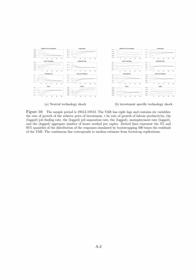
In discussing the results for panel (b), one should bear in mind two important

facts (see Figures 10 and 11 in the Appendix): i) the estimated responses in the

first subsample are almost never significant (with the exception of the response of the

relative price of investment) and ii) investment specific technology shocks contribute

10

little to the volatility of all variables in the first subsample (again leaving aside the

price of investment). In the second sub-period the contribution of investment specific

shocks instead becomes important. Hence, it is appropriate to compare estimates for

the full sample and the 1973:2-1997:1 sub-period. The bias in the estimated responses

for the full sample is in line with the low frequency correlations previously discussed.

In the full sample, a permanent change in the rate of growth of the relative price of

investment is at least partly identified as a series of investment specific technology

shocks. Thus, over the period 1973:II-1997:I when the price of investment falls at a

faster rate on average, the full sample specification tends to identify a series of positive

investment specific technology shocks. Since over the period, the unemployment rate

and the separation rate are also higher than their full sample average, while hours, the

job finding rate, and productivity growth are lower, the full sample specification biases

estimates towards a higher response of the unemployment rate and of the separation

rate, and a lower response of hours, the job finding rate, and productivity.

2.4 Discussion

The above results are robust to a number of standard modifications. For example,

they are unaffected if the second subsample is 1973:II-2000:IV (see panels (a) and (b)

in Figure 12 in the Appendix) or if we use the population-adjusted hours of Francis

and Ramey (2005) instead of the standard per-capita hours series.

Commentators have sometimes questioned our choice of break points. Some have

suggested that taking a break point as known (when in fact it is not) may bias results,

while others have suggested that a perhaps more relevant break point would be, as in

the Great Moderation literature, somewhere around the beginning of 1980. Figures 13

and 14 in the Appendix show that moving backward or forward by one year the two

chosen break dates does not change the conclusion that, over subsamples, the responses

of the variables are similar and different from those of the full sample. Concerning the

break around the beginning of the 1980s, visual inspection of Figure 1 clearly indicates

that none of the series we consider displays any unusual behavior around that date.

One interpretation of this evidence is that, if the events driving the rise and fall of

inflation, its volatility and persistence matter for labor market variables, they must

matter at much longer run frequencies.

11

The evidence in Figure 3 indicates that the dynamic responses of the variables of

the VAR to the two shocks are very much homogeneous over subsamples. Therefore,

the low frequency variations we have highlighted imply that the constant of the VAR

needs to be adjusted and this is what we do in this paper. In Canova et al. (2006),

we elaborate on this issue and present cases where unaccounted level breaks within a

sample produce sign switches or an extreme pattern of persistence in the responses. It

could be argued that a simple way to eliminate the low frequency comovements is to

estimate the VAR over sub-samples, but this would be inefficient, since the dynamics

are roughly unchanged, and it may cause biases, since imposing long run restrictions

in a system estimated over a small sample distorts structural estimates (see Erceg et

al. 2005).

It goes without saying that low frequency movements in the data are the object

of controversial discussion and our choice of eliminating them could be criticized in,

at least, two ways. It could be argued, for example, that after a prolonged period

of low productivity growth and in anticipation that productivity will pick up, labor

input could be lower in the low productivity period, making low frequency movements

informative about business cycle fluctuations. One way to rationalize our decision of

removing low frequency fluctuations is that breaks can not be forecasted so anticipatory

effects are not present. It could also be argued that changes in productivity growth also

affect agents decisions rule. This would imply that one can get mistaken conclusions

from estimating the model for the full sample, just allowing changes in the intercept.

This argument is theoretically correct but it does not appear to hold in the data.

The dynamics in response to the shocks are very similar in the two subsamples (and

different from the full sample where no adjustment for low frequency movements is

made) so agent’s decision rules appear to be unaffected by the breaks. Furthermore,

we will show below that, once breaks in the intercepts are considered, the full sample

evidence coincides with the sub-sample one.

12

3 The results

3.1 Evidence using the approximated rates

Panel (a) in Figure 4 plots the response of the variables of interest to a neutral tech-

nology shock when the VAR includes the approximated job finding and job separation

rates and the intercept is deterministically broken at 1973:2 and 1997:1. The reported

bands correspond to 90 percent confidence intervals. A neutral shock leads to an in-

crease in unemployment and to a fall in the aggregate number of hours. The effects

on hours worked per employee are small and, generally, statistically insignificant. The

impact increase in unemployment is the result of a sharp rise in the separation rate

and of a significant fall in the job finding rate. In the quarters following the shock,

Neutral ShockRelative Price of Investment

5 10 15 20 250.00

0.05

0.10

0.15

0.20

Labor Productivity

5 10 15 20 250.18

0.36

0.54

0.72

0.90

Unemployment

5 10 15 20 250.0

1.6

3.2

4.8

Hours

5 10 15 20 25-0.6

-0.4

-0.2

-0.0

0.2

Finding Rate

5 10 15 20 25-4.8

-3.2

-1.6

-0.0

Separation Rate

5 10 15 20 25-0.5

0.0

0.5

1.0

1.5

2.0

Hours per Employee

5 10 15 20 25-0.36

-0.27

-0.18

-0.09

-0.00

0.09

Output

5 10 15 20 25-0.25

0.00

0.25

0.50

0.75

1.00

Investment Specific ShockRelative Price of Investment

5 10 15 20 25-1.12

-0.96

-0.80

-0.64

-0.48

-0.32

Labor Productivity

5 10 15 20 25-0.32

-0.24

-0.16

-0.08

0.00

0.08

Unemployment

5 10 15 20 25-2.4

-1.6

-0.8

-0.0

0.8

Hours

5 10 15 20 250.00

0.25

0.50

0.75

Finding Rate

5 10 15 20 25-1.8

-0.9

0.0

0.9

1.8

Separation Rate

5 10 15 20 25-2.5

-2.0

-1.5

-1.0

-0.5

0.0

Hours per Employee

5 10 15 20 250.0

0.2

0.4

0.6

Output

5 10 15 20 25-0.35

0.00

0.35

0.70

(a) Neutral technology shock (b) Investment specific technology shock

Figure 4: Responses to a one-standard deviation shocks. Full sample with intercept deterministi-cally broken at 1973:II and 1997:I. Six variables VAR(8). Dotted lines are 5% and 95% quantiles ofthe distribution of the responses simulated by bootstrapping 500 times the residuals of the VAR. Thecontinuous line is the median estimate.

the separation rate returns to normal levels while the job finding rate takes up to fif-

teen quarters to recover. Hence, the dynamics of the job finding rate explains why

unemployment responses are persistent. Output takes about 5 quarters to significantly

13

respond but then gradually increases until it reaches its new higher long-run value.

Note that the dynamic responses for the full sample in Figure 4 now look like those of

the two subsamples we reported in Figure 3.

Panel (b) in Figure 4 plots responses to an investment specific shock. The responses

are very similar to those obtained in the 1973:2-1997:1 sub-sample presented in Figure

3. An investment specific technology shock leads to a short run increase in output and

hours per capita and a fall in unemployment. The fall of unemployment on impact

is due to a sharp drop in the separation rate. Since this effect is partly compensated

by a fall in the job finding rate, the initial fall in unemployment rate is small in

absolute terms and statistically insignificant. Consequently, the increase in hours is

primarily explained by the sharp and persistent increase in the number of hours worked

per employee. Hence, while labor market adjustments to neutral technology shocks

occur mainly along the extensive margin, those in response to an investment specific

technology shock mainly occur along the intensive margin.

3.2 Evidence using the exact rates

We next use exact job finding and separation rates in the VAR. Panel (a) in Figure

5 presents the responses to a neutral technology shock with the exact rate (dotted

line) together with the previously discussed responses obtained with the approximated

rates (solid line). The sign and shape of the responses are similar with both specifi-

cations. There are however two important quantitative differences. When considering

the exact rates, the separation rate rises on impact twice as much, while the finding

rate falls slightly less and, over the adjustment path, the separation rate exhibits more

persistence when exact rates are used.

Panel (b) in Figure 5 reports responses to an investment specific technology shock

when exact and approximated rates are used. Also in this case, the two specifications

agree on the sign and shape of the responses. However, there are two significant

quantitative differences. When the exact rates are used, the response of the separation

rate is more pronounced and falls on impact twice as much. Instead, the job finding rate

is now unaffected on impact and remains above normal levels all along the adjustment

path. As a result, the fall in the unemployment rate is more pronounced both on

impact and during the transition — the extensive margin plays a more important role

14

Neutral ShockRelative Price of Investment

5 10 15 20 25-0.025

0.000

0.025

0.050

0.075

0.100

Labor Productivity

5 10 15 20 250.4

0.5

0.6

0.7

0.8

0.9

Unemployment

5 10 15 20 250

1

2

3

4

5

Hours

5 10 15 20 25-0.64

-0.48

-0.32

-0.16

0.00

Finding Rate

5 10 15 20 25-4.2

-2.8

-1.4

0.0

Separation Rate

5 10 15 20 250.0

1.2

2.4

3.6

Hours per Employee

5 10 15 20 25-0.36

-0.24

-0.12

0.00

Output

5 10 15 20 25-0.25

0.00

0.25

0.50

0.75

1.00

Investment Specific ShockRelative Price of Investment

5 10 15 20 25-1.4

-1.2

-1.0

-0.8

-0.6

-0.4

Labor Productivity

5 10 15 20 25-0.36

-0.24

-0.12

0.00

Unemployment

5 10 15 20 25-2.1

-1.4

-0.7

0.0

Hours

5 10 15 20 250.0

0.2

0.4

0.6

Finding Rate

5 10 15 20 25-1.0

-0.5

0.0

0.5

1.0

1.5

Separation Rate

5 10 15 20 25-3

-2

-1

0

Hours per Employee

5 10 15 20 250.00

0.16

0.32

0.48

Output

5 10 15 20 25-0.32

-0.16

0.00

0.16

0.32

0.48

(a) Neutral technology shock (b) Investment specific technology shock

Figure 5: Exact rates (dotted lines) and approximated rates (solid lines). Both VAR includesdummies corresponding to the breaks in technology growh. Each VAR has 8 lags and six variables.Reported are point estimates of the responses.

in accounting for the rise in hours when exact rates are used.

3.3 Omitted variables

Our VAR has enough lags to make the residuals clearly white noises. Yet, it is possible

that omitted variables play a role in the results. For example, Evans (1992) showed

that Solow residuals are correlated with a number of policy variables, therefore making

responses to Solow residuals shocks uninterpretable. To check for this possibility we

have correlated our two estimated technology shocks with variables which a large class

of general equilibrium models suggest as being jointly generated with neutral and

investment specific shocks. We compute correlations up to 6 leads and lags between

each of our technology shocks and the consumption to output ratio, the investment to

output ratio, and the inflation rate. The point estimates of these correlations together

with an asymptotic 95 percent confidence tunnel around zero are in Figure 6. The

shocks we use are those obtained in the VAR with the approximated rates, but the

results are similar when exact rates are used.

15

Correlation with omitted variablesNeutral shock

c/y ratio

-6 -4 -2 0 2 4 6-0.50

-0.25

0.00

0.25

0.50

i/y ratio

-6 -4 -2 0 2 4 6-0.50

-0.25

0.00

0.25

0.50

inflation

-6 -4 -2 0 2 4 6-0.50

-0.25

0.00

0.25

0.50

Investment shockc/y ratio

-6 -4 -2 0 2 4 6-0.50

-0.25

0.00

0.25

0.50

i/y ratio

-6 -4 -2 0 2 4 6-0.50

-0.25

0.00

0.25

0.50

inflation

-6 -4 -2 0 2 4 6-0.50

-0.25

0.00

0.25

0.50

Figure 6: Left column corresponds to neutral technology shocks; right column to investment specifictechnology shocks. The first row plots the correlation with the consumption-output ratio, the secondwith the investment-output ratio, the third with the inflation rate. The shocks are estimated from

the six variables VAR with approximated rates in the dummy specification. The horizontal linescorrespond to an asymptotic 95 percent confidence interval for the null of zero correlation.

The consumption to output and the investment to output ratios help to predict

neutral technology shocks at some horizon, while none of the three potentially omitted

variables significantly correlate with investment specific shocks. Hence, we investigate

what happens when we enlarge the system to include these three new variables. Panels

(a) and (b) in Figure 15 in the Appendix present the responses in VAR which includes

the original six variables (approximate rates are used) plus the consumption to output

and the investment to output ratios and the inflation rate. None of our previous

conclusions regarding the dynamics of labor market variables is affected.

4 The role of separation rates

Hall (2005) and Shimer (2007) have challenged the conventional view that recessions–

defined as periods of sharply rising unemployment–are the result of higher job-loss

rates. They argue that recessions are mainly explained by a fall in the job finding rate.

Our responses suggest instead that the separation rate plays a major role in determining

16

the impact effect of technology shocks on unemployment. This is consistent with the

evidence of Fujita and Ramey (2006) that the separation rate leads the cycle (by about

one quarter) while the finding rate lags it (by about two months).

To further evaluate the role of the separation rate for unemployment fluctuations,

we use a simple two state model of the labor market (see Jackman et al. (1989) and

Shimer (2007) and (2008)) and assume that the stock of unemployment evolves as:

ut = S(lt − ut)− Fut (1)

where lt and ut are the size of the labor force and the stock of unemployment, respec-

tively; while S and F are the separation and finding rates in levels, respectively. The

unemployment rate tends to converge to the following fictional unemployment rate:

u =S

S + F≡ exp(s)

exp(s) + exp(f).

Shimer (2007) shows that the fictional unemployment rate u tracks quite closely the

actual unemployment rate series, so that one can fully characterize the evolution of the

stock of unemployment just by characterizing the dynamics of labor market flows. After

linearizing the log of u, we can calculate its response using the information contained

in the response of (the log of) the separation rate s and the finding rate f. This

simple setup allows to measure the contribution of finding and separation rates to the

cyclical fluctuations of fictional unemployment u and evaluate how accurately fictional

unemployment approximates actual unemployment (if it does workers movements in

and out of the labor force play a minor role for unemployment fluctuations).

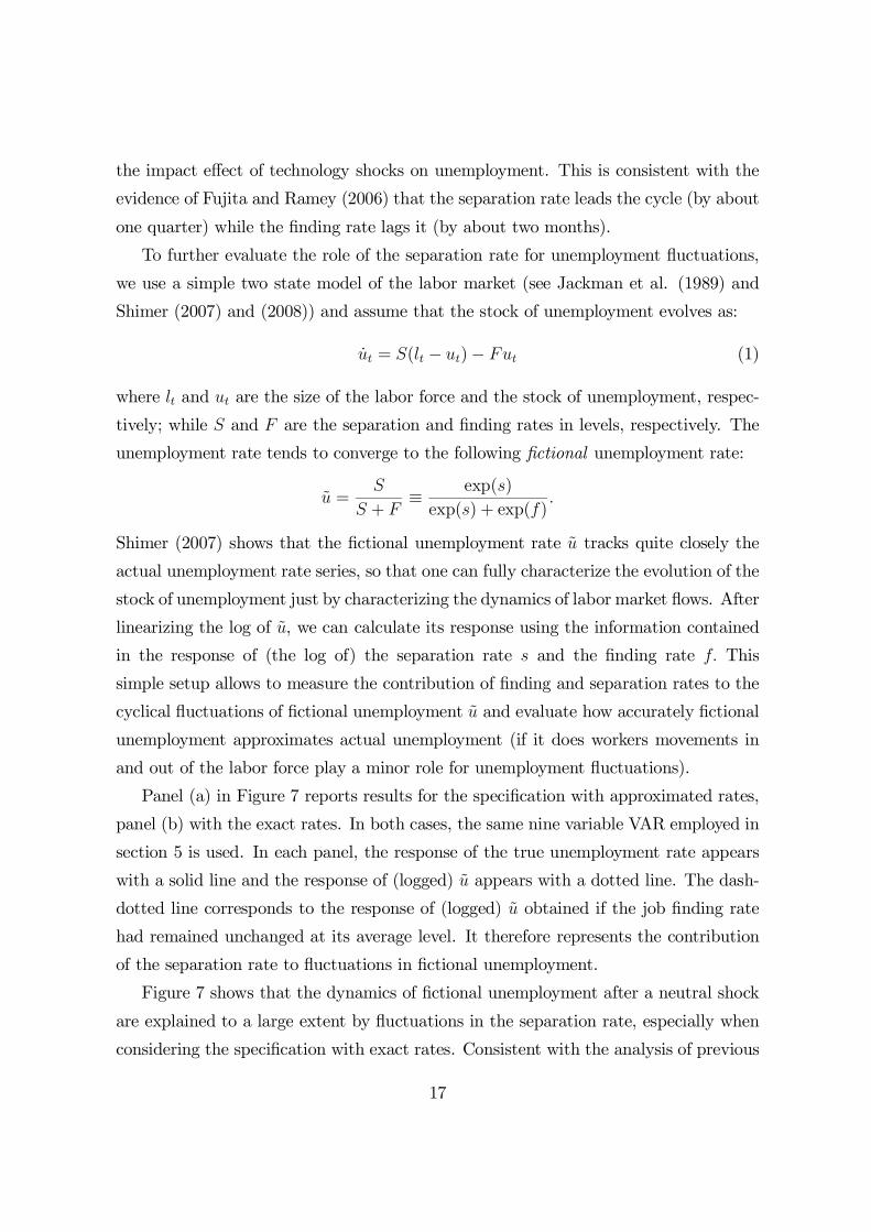
Panel (a) in Figure 7 reports results for the specification with approximated rates,

panel (b) with the exact rates. In both cases, the same nine variable VAR employed in

section 5 is used. In each panel, the response of the true unemployment rate appears

with a solid line and the response of (logged) u appears with a dotted line. The dash-

dotted line corresponds to the response of (logged) u obtained if the job finding rate

had remained unchanged at its average level. It therefore represents the contribution

of the separation rate to fluctuations in fictional unemployment.

Figure 7 shows that the dynamics of fictional unemployment after a neutral shock

are explained to a large extent by fluctuations in the separation rate, especially when

considering the specification with exact rates. Consistent with the analysis of previous

17

section, the separation rate explains almost 90 per cent of the impact effect on fictional

unemployment. However, its contribution falls to 40 per cent after one quarter and

drops to 20 per cent one year after the shock. There are some differences in the impact

response of actual and fictional unemployment. Hence, workers movements in and out

of the labor force play some role in characterizing the response of the unemployment

rate, at least on impact.

Contribution of Separation rateu (continuous), u-fictional (dotted), Separation only (dash-dotted)

Neutral Shock

5 10 15 20 25-0.9

0.0

0.9

1.8

2.7

Investment Specific Shock

5 10 15 20 25-0.96

-0.80

-0.64

-0.48

-0.32

-0.16

Contribution of Separation rateu (continuous), u-fictional (dotted), Separation only (dash-dotted)

Neutral Shock

5 10 15 20 25-0.9

0.0

0.9

1.8

2.7

Investment Specific Shock

5 10 15 20 25-1.25

-1.00

-0.75

-0.50

-0.25

0.00

(a) Approximated rates (b) Exact rates

Figure 7: Nine variables VAR with approximated or exact rates. Full sample with deterministictime dummies. Reported are median estimates from 500 bootstrap replications.

Following an investment specific shock, when approximated rates are used, unem-

ployment falls little on impact because the fall in the separation rate makes unem-

ployment decrease while the fall in the job finding rate makes unemployment increase.

When considering the specification with exact rates, unemployment falls substantially

on impact and this is mainly due to the fall in the separation rate. Since the differ-

ences between the response of fictional and actual unemployment are minimal, both

with approximated and with exact rates, adjustments in others labor market flows are

small in responses to these shocks.

5 The contribution of technology shocks

To put our findings in the right perspective, it is necessary to show that the contribu-

tion of technology shocks to fluctuations in the variables of interest is non-negligible.

Otherwise, what we uncover is an interesting intellectual curiosity without practical

implications. Table 1 reports the forecast error variance decomposition using either

18

the approximated rates or the exact rates. We present results for the VAR with nine

variables for the full sample and for the subsample 1973:II-2000:IV. If the consumption

and the investment to output ratio, and the inflation rate are omitted, the contribution

of technology shocks is marginally larger (on average by about ten percentage points).

In the specification with approximated rates, neutral technology shocks explain

about 20 per cent of unemployment fluctuations at time horizons between 4 and 8

years while the contribution to the forecast error variance of hours per worker is only

five per cent. Investment specific technology shocks instead account for a substantial

proportion of the volatility of hours worked: around 20 per cent of the volatility of hours

per capita and 30 per cent of the volatility of hours per worker. Their contribution to

unemployment volatility is instead small (generally smaller than 10 per cent). Taken

together, technology shocks explain a relevant proportion of the labor market volatility:

at horizons between 2 and 8 years they explain around 30 per cent of the volatility of

unemployment and hours.

The importance of technology shocks is somewhat larger when exact rates are used

(see panel C). This is however due to the greater importance of technology shocks in

the 1973:II-2000:IV sample period. When we estimate the VAR with approximated

rates in the 1973:II-2000:IV sample, we find that technology shocks explain roughly

the same amount with approximated and exact rates (see panel B). The main exception

is in the contribution of neutral technology shocks to the volatility of the separation

rate, which is three times larger with exact rates.

Further evidence on the role of technology shocks in generating cyclical fluctua-

tions can be obtained looking at the historical contribution of technology shocks to

fluctuations in the log of unemployment, hours, job finding and job separation rates.

The graphs in Figure 8 represent with a solid line the original series and with a dotted

line its component due to technology shocks (either neutral or investment specific), as

recovered from the nine variables VAR with the exact rates. All series are detrended

with a Hodrick Prescott filter with smoothing parameter equal to 1600. The areas in

grey correspond to the NBER recessions.

It is apparent that technology shocks are an important driving force of cyclical fluc-

tuations in labor market variables, probably more so for unemployment than for hours.

They account for several important business cycle episodes, including the recession of

19

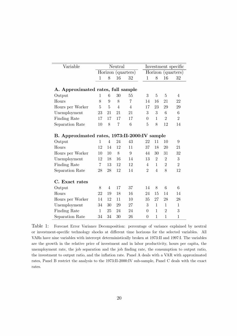
Variable Neutral Investment specificHorizon (quarters) Horizon (quarters)1 8 16 32 1 8 16 32

A. Approximated rates, full sampleOutput 1 6 30 55 3 5 5 4Hours 8 9 8 7 14 16 21 22Hours per Worker 5 5 4 4 17 23 29 29Unemployment 23 21 21 21 3 3 6 6Finding Rate 17 17 17 17 0 1 2 2Separation Rate 10 8 7 6 5 8 12 14

B. Approximated rates, 1973:II-2000:IV sampleOutput 1 4 24 43 22 11 10 9Hours 12 14 12 11 37 18 20 21Hours per Worker 10 10 8 9 44 30 31 32Unemployment 12 18 16 14 13 2 2 3Finding Rate 7 13 12 12 4 1 2 2Separation Rate 28 28 12 14 2 4 8 12

C. Exact ratesOutput 8 4 17 37 14 8 6 6Hours 22 19 18 16 24 15 14 14Hours per Worker 14 12 11 10 35 27 28 28Unemployment 34 30 29 27 3 1 1 1Finding Rate 1 25 24 24 0 1 2 3Separation Rate 34 34 30 26 0 1 1 1

Table 1: Forecast Error Variance Decomposition: percentage of variance explained by neutralor investment-specific technology shocks at different time horizons for the selected variables. All

VARs have nine variables with intercept deterministically broken at 1973:II and 1997:I. The variablesare the growth in the relative price of investment and in labor productivity, hours per capita, theunemployment rate, the job separation and the job finding rate, the consumption to output ratio,the investment to output ratio, and the inflation rate. Panel A deals with a VAR with approximatedrates, Panel B restrict the analysis to the 1973:II-2000:IV sub-sample, Panel C deals with the exact

rates.

20

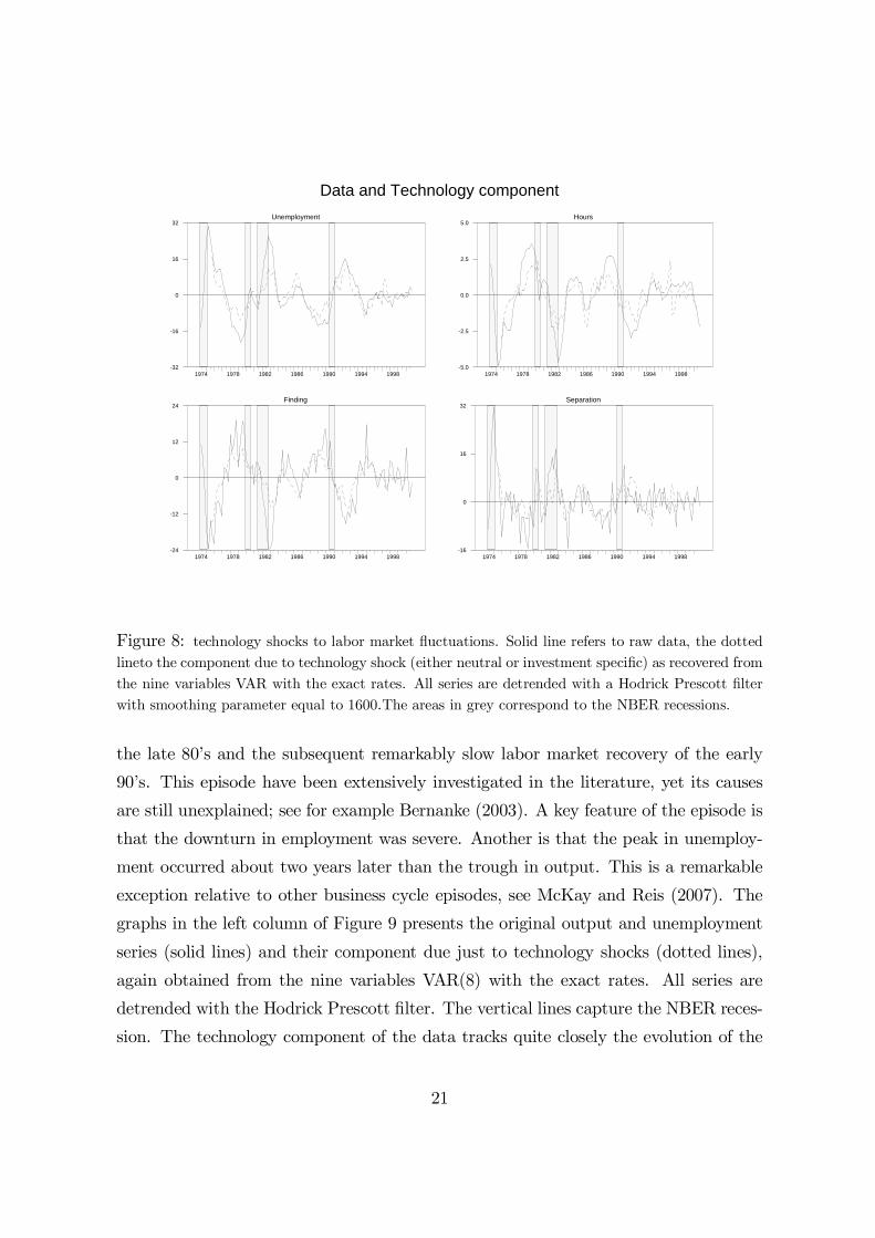
Data and Technology componentUnemployment

1974 1978 1982 1986 1990 1994 1998-32

-16

0

16

32

Finding

1974 1978 1982 1986 1990 1994 1998-24

-12

0

12

24

Hours

1974 1978 1982 1986 1990 1994 1998-5.0

-2.5

0.0

2.5

5.0

Separation

1974 1978 1982 1986 1990 1994 1998-16

0

16

32

Figure 8: technology shocks to labor market fluctuations. Solid line refers to raw data, the dottedlineto the component due to technology shock (either neutral or investment specific) as recovered fromthe nine variables VAR with the exact rates. All series are detrended with a Hodrick Prescott filterwith smoothing parameter equal to 1600.The areas in grey correspond to the NBER recessions.

the late 80’s and the subsequent remarkably slow labor market recovery of the early

90’s. This episode have been extensively investigated in the literature, yet its causes

are still unexplained; see for example Bernanke (2003). A key feature of the episode is

that the downturn in employment was severe. Another is that the peak in unemploy-

ment occurred about two years later than the trough in output. This is a remarkable

exception relative to other business cycle episodes, see McKay and Reis (2007). The

graphs in the left column of Figure 9 presents the original output and unemployment

series (solid lines) and their component due just to technology shocks (dotted lines),

again obtained from the nine variables VAR(8) with the exact rates. All series are

detrended with the Hodrick Prescott filter. The vertical lines capture the NBER reces-

sion. The technology component of the data tracks quite closely the evolution of the

21

Figure 9: The jobless recovery of the 90s. Solid lines are raw data (either unemployment, findingrates, separation rates or output), the dotted lines the component due to technology shocks (eitherneutral or investment specific) as recovered from the nine variables VAR with the exact rates. Allseries are detrended with a Hodrick Prescott filter with smoothing parameter equal to 1600. Thevertical lines identifies the NBER recession.

raw data. This is mainly due to the evolution of neutral shocks that naturally tend to

induce jobless recoveries: following the initial rise in job separation and unemployment,

output increases to its new higher long run value, while unemployment remains above

trend because of the low job finding rate, which induces a remarkably slow recovery in

the labor market, see the right column of figure 9.

6 An interpretation

Our findings indicate that the separation rate is important in characterizing the labor

market response to technology shocks. We also find that labor market adjustments to

different types of technology shocks are different. Neutral shocks exercise their effects

primarily along the extensive margin of the labor market; investment specific shocks

along the intensive margin. Moreover, neutral shocks create unemployment, while

investment specific shocks increase labor input. These results have important implica-

tions for both empirical analysis concerning sources of business cycle fluctuations and

theoretical models designed to explain them.

First, failure to empirically distinguish between the two types of disturbances may

lead to nonsensical representation of the dynamics following unexpected technological

22

improvements. Second, our results qualify the conclusions by Hall (2005) and Shimer

(2007) and show the importance of using search models with endogenous separation for

business cycle analysis. The difference in conclusions is due to our focus on correlations

conditional on technology shocks, rather than on unconditional correlations at generic

business cycle frequencies. Third, for interpretation purposes, it is very important

to separate the extensive from the intensive margin of labor market and just using

total hours may lead to distortions in the analysis. For example, it is well known

that hours fall in response to neutral technology shocks and starting with Galí (1999)

it is common to interpret this evidence using sticky prices models. In sticky-price

models, when technology improves and monetary policy is not accommodating enough,

demand is sluggish to respond to the shocks and firms take advantage of technology

improvements to economize on labor input. While this mechanism has its own appeal,

it most naturally applies to the intensive margin of the labor market since displacing

workers must be more costly than changing prices when cost of displacement includes

both the direct cost of firing and the value of the sunk investment in training and in job

specific human capital that is lost with firing (see e.g. Mankiw, 1985 and Hamermesh,

1993 for a review of the literature). Admittedly, no formal model analyzing the trade-

off between changing prices and displacing workers exists in the literature but one can

conjecture that when the decision of changing prices is endogenous and menu cost a-la

Caballero and Engel (2007) are used, this is the expected outcome. The evidence we

have provided indicates instead that labor market adjustments to neutral shocks occur

primarily at the extensive margin and the fall in hours is mostly caused by the time

consuming process of reallocation of workers across productive units.

A possible alternative interpretation of our finding is that investment specific tech-

nological progress has standard neoclassical features, while the transmission of neutral

shocks is consistent with the Schumpeterian view that the introduction of new neutral

technologies causes the destruction of technologically obsolete productive units and the

creation of new technologically advanced ones. When the labor market features search

frictions, this process leads to a temporary rise in unemployment. Schumpeterian cre-

ative destruction matters for productivity dynamics at the micro level, see Foster et

al. (2001) and it is a prominent paradigm in the growth literature, see Aghion and

Howitt (1994), Mortensen and Pissarides (1998), Violante (2002) and Hornstein et al.

23

(2005). Caballero and Hammour (1994, 1996) and Michelacci and Lopez-Salido (2007)

show how such a paradigm may also be relevant for business cycle analysis.

7 Robustness

This section briefly describes some robustness exercises we have undertaken. The

conclusion is that our technology shocks are unlikely to stand in for other sources

of disturbances and that our conclusions remain when we change i) the lag length

of the VAR, ii) the way we remove low frequency fluctuations, iii) the timing of the

identification restrictions, iv) the price deflator, and v) the labor market data and the

series for the relative price of investment.

Other disturbances Despite the fact that our technology shocks do not proxy

for omitted variables, it is still possible that they stand in for other sources of dis-

turbances. To check for this possibility, we have correlated the estimated technology

shocks obtained from the nine variables VAR with the approximated rates with oil

prices (mnemonics PZTEXP) deflated by the consumption deflator and federal fund rate

shocks (FFED), the latter computed filtering FFED with an AR(1). Figure 16 in the

Appendix shows that correlations are insignificant.

VAR lag length The issue of the length of VAR has been recently brought back

to the attention of applied researchers by Giordani (2004) and Chari et al. (2008),

who show that the aggregate decision rules of a subset of the variables of a model

may have not always be representable with a finite order VAR. This issue is unlikely

to be important in our context since we have checked that the residuals of a VAR(8)

are white noise and do not stand-in for other potential sources of shocks. To further

investigate whether this is an issue, we have reestimated our VAR using 4 and 12 lags.

The results using approximated rates are in Figure 18 in the Appendix. The pattern of

responses is unchanged. Our results are independent of the chosen lag length because

the stochastic decay restriction we use effectively removes the noise that longer lags

tend to produce in the VAR.

24

Alternative treatments of trends We have considered two alternatives to re-

move low frequency movements in the variables of the VAR: we have allowed up to a

fifth order polynomial in time as intercept in the VAR; we filtered all the variables,

before entering them in the VAR, with the Hodrick Prescott filter with a smoothing

parameter λ = 10000. Figure 17 in the Appendix show that responses have the same

shape and approximately the same size as with our benchmark specification.

Medium versus long-run identifying restrictions Uhlig (2004) has argued

that disturbances other than neutral technology shocks may have long run effects on

labor productivity and that, in theory, there is no horizon at which neutral (and invest-

ment specific) shocks fully account for the variability of labor productivity. Literally,

this implies the neutral shocks we have extracted may not be structural. To take care

of this problem Uhlig suggests to check if conclusions change when medium term re-

strictions are used. In Panel (a) and (b) of Figure 19 in the Appendix we report the

responses obtained when the restrictions that the two shocks are the sole source of

fluctuations in labor productivity and the price of investment is imposed at the time

horizon of 3 years rather than in the long-run. The sign and the shape of responses

are almost unchanged. Similar results are obtained if the restrictions are imposed at

any horizon of at least one year.

Price deflators In our benchmark VAR, labor productivity and the relative price

of investment are deflated with the output deflator. Intuitively, using this deflator is

equivalent to use domestic consumption as a numeraire. As we previously mentioned,

other authors have either used the CPI deflator or combination of output and CPI

deflators. Such choice is potentially problematic since the identifying assumptions we

employ are no longer valid using such deflators.

To see this recall that when the price of investment and total factor productivity

have unit roots, a standard Solow economy evolves around the (stochastic) trend

X ≡ Z1

1−α Qα

1−α

where Z is the TFP component and Q the price of investment component (see e.g.

Michelacci and Lopez-Salido (2007)) and that the quantities Y ≡ Y / (XN) , and K ≡

25

K/ (XQN) converge to Y ∗ = (s/δ)α

1−α andK∗ = (s/δ)1

1−α , respectively. Consequently,

the logged level of aggregate productivity, yn ≡ ln Y /N , evolves according to

yn = y∗ + v + x = y∗ + v +1

1− αz +

α

1− αq (2)

where small letters denote the log of the corresponding quantities in capital letters and

v is a stationary term which accounts for transitional dynamics. Hence, in this case,

the long run component of labour productivity is entirely due to the neutral and the

investment specific shock.

Now, let qc and ycn denote the inverse of the relative price of investment and labor

productivity (both in logs), when deflated with the Consumer Price Index , Pc, defined

as Pc =³PHc

a

´a ³PFc

1−a

´1−a, where PH

c and PFc are the prices of consumption goods

produced in the US and abroad; and a represents the share of domestic consumption

goods. Tedious calculations show that

ycn = cte+1

1− α− βz +

α + β

1− α− βqc +

1

1− α − β(1− a)

¡pHc − pFc

¢(3)

where α and β are the output elasticities to domestic and foreign capital, respectively.

Hence, with this choice of numeraire, a permanent change in the real exchange rate

could affect long run labor productivity and confused with “neutral” technology shocks

(see also Kehoe and Ruhl (2007)). Since the real exchange rate exhibits remarkable

persistence, one should worry about mixing neutral and real exchange rate shocks.

When we deflate the relative price of investment with the CPI index and output

with the GDP deflator we obtain

yn = cte+1

1− α− βz +

α + β

1− α− βqc +

α+ β

1− α − β(1− a)

¡pHc − pFc

¢,

and, again, a permanent change in pHc − pFc has long run effects on productivity.

Our choice of deflator is the right one, in the sense that it implies a well defined

balanced growth path in an open economy version of the Solow model, and does not

suffer from misspecification issues. Nevertheless, it is worth investigating whether the

results we obtain would be strongly altered if these alternatively deflators would be

used. We have therefore computed responses for the VAR with approximated rates

deflating output and the price of investment by the CPI (see Figures 20 in the Ap-

pendix). Responses are roughly similar to our benchmark ones. The main difference

26

concerns the response of the price of investment to a neutral technology shock, which

is more pronounced in this latter case.

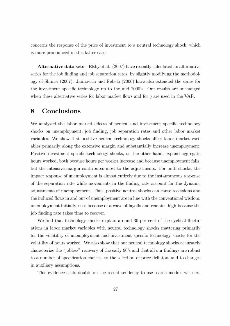
Alternative data sets Elsby et al. (2007) have recently calculated an alternative

series for the job finding and job separation rates, by slightly modifying the methodol-

ogy of Shimer (2007). Jaimovich and Rebelo (2006) have also extended the series for

the investment specific technology up to the mid 2000’s. Our results are unchanged

when these alternative series for labor market flows and for q are used in the VAR.

8 Conclusions

We analyzed the labor market effects of neutral and investment specific technology

shocks on unemployment, job finding, job separation rates and other labor market

variables. We show that positive neutral technology shocks affect labor market vari-

ables primarily along the extensive margin and substantially increase unemployment.

Positive investment specific technology shocks, on the other hand, expand aggregate

hours worked, both because hours per worker increase and because unemployment falls,

but the intensive margin contributes most to the adjustments. For both shocks, the

impact response of unemployment is almost entirely due to the instantaneous response

of the separation rate while movements in the finding rate account for the dynamic

adjustments of unemployment. Thus, positive neutral shocks can cause recessions and

the induced flows in and out of unemployment are in line with the conventional wisdom:

unemployment initially rises because of a wave of layoffs and remains high because the

job finding rate takes time to recover.

We find that technology shocks explain around 30 per cent of the cyclical fluctu-

ations in labor market variables with neutral technology shocks mattering primarily

for the volatility of unemployment and investment specific technology shocks for the

volatility of hours worked. We also show that our neutral technology shocks accurately

characterize the “jobless” recovery of the early 90’s and that all our findings are robust

to a number of specification choices, to the selection of price deflators and to changes

in auxiliary assumptions.

This evidence casts doubts on the recent tendency to use search models with ex-

27

ogenous separation rates to analyze the effects of technology shocks and qualifies the

conclusions by Hall (2005) and Shimer (2007). It also challenges the standard sticky

price explanation for why hours fall in response to neutral technology shocks, since

the mechanism emphasized in these models primarily applies to the intensive mar-

gin, while we find that the extensive margin plays a key role in the adjustment. The

evidence may instead be consistent with the idea that investment specific technologi-

cal progress has standard neoclassical features, while neutral technological progress is

Schumpeterian. According to this view the introduction of new neutral technologies

causes the destruction of technologically obsolete productive units and the creation of

new technologically advanced ones. When the labor market is characterized by search

frictions, these adjustments lead to a temporary rise in unemployment.

28

References[1] Aghion, P. and Howitt, P. (1994): “Growth and Unemployment,” Review of Eco-

nomic Studies, 61, 477-494.

[2] Altig, D. Christiano, J. Eichenbaum, M. and Linde, J. (2005): “Firm-SpecificCapital, Nominal Rigidities and the Business Cycle,” NBERWorking Paper 11034.

[3] Bernanke, B. (2003): “The Jobless Recovery. Remarks by Governor BenBernanke,” speech at the Global Economic and Investment Outlook Conference.Available at www.federalreserve.gov/boarddocs/speeches.

[4] Blanchard, O. and Diamond, P. (1990): “The Cyclical Behavior of the Gross Flowsof U.S. Workers,” Brookings Papers on Economic Activity, 2, 85—143.

[5] Blanchard, O. and Quah, D. (1989): “The Dynamic Effects of Aggregate Demandand Supply Disturbances,” American Economic Review, 79, 655-673.

[6] Caballero, R. and Hammour, M. (1994): “The Cleansing Effect of Recessions,”American Economic Review, 84, 1350-1368.

[7] Caballero, R. and Hammour, M. (1996): “On the Timing and Efficiency of Cre-ative Destruction,” Quarterly Journal of Economics, 111, 805-852.

[8] Caballero, R. and Engel, E. (2007): “Price Stickiness in Ss Models: New Interpre-tations of Old Results,” Mimeo, MIT and Yale University.

[9] Canova, F. López-Salido, D. and Michelacci, C. (2006): “On the Robust Effectsof Technology Shocks on Hours worked and Output,” mimeo UPF.

[10] Chari, V. , Kehoe, P. and McGrattan, E. (2008): “A critique of SVAR using RealBusiness Cycle theory,” Journal of Monetary Economics, forthcoming.

[11] Cummins, J. and Violante, G. (2002): “Investment Specific Technical Change inthe US (1947-2000): Measurement and Macroeconomic Consequences,” Review ofEconomic Dynamics, 5, 243-284.

[12] Darby, M., J. Haltiwanger, and Plant, M. (1985): “Unemployment Rate Dynamicsand Persistent Unemployment under Rational Expectations,” American EconomicReview, 75(4): 614—637.

[13] Darby, M., J. Haltiwanger, and Plant, M. (1986): “The Ins and Outs of Unem-ployment: The Ins Win,” NBER Working Paper.

[14] Elsby, M., Michaels, R. and Solon, G. (2007): “The Ins and Outs of CyclicalUnemployment,” AEJ: Macroeconomics, forthcoming.

29

[15] Fernald, J. (2007): “Trend Breaks, Long Run Restrictions, and ContractionaryTechnology Improvements,” Journal of Monetary Economics, forthcoming.

[16] Fisher, J. (2006): “The Dynamic Effects of Neutral and Investment-Specific Tech-nology Shocks,” Journal of Political Economy, 114, 413-451.

[17] Foster, L., Haltiwanger, J. and Krizan, C. (2001): “Aggregate ProductivityGrowth: Lessons from Microeconomic Evidence,” in New Developments in Pro-ductivity Analysis, University of Chicago Press.

[18] Francis, N. and Ramey, V. (2005): “Is the Technology-Driven Real Business Cy-cle Hypothesis Dead? Shocks and Aggregate Fluctuations Revisited,” Journal ofMonetary Economics, 52, 1379-1399.

[19] Fujita, S. and Ramey, G. (2006): “The Cyclicality of Job Loss and Hiring,” Mimeo,Federal Reserve Bank of Philadelphia.

[20] Galí, J. (1999): “Technology, Employment, and the Business Cycle: Do Technol-ogy Shocks Explain Aggregate Fluctuations?,” American Economic Review, 89,249-271.

[21] Galí, J. and Rabanal, P. (2004): “Technology Shocks and Aggregate Fluctuations:How Well Does the RBC Model Fit Postwar U.S. Data?”, NBER MacroeconomicsAnnual, 19, 225-288.

[22] Giordani, P. (2004): “An Alternative Explanation of the Price Puzzle,” Journalof Monetary Economics, 51, 1271-1296.

[23] Gordon, R. (2000): “Does the ‘New Economy’ Measure Up To The Great Inven-tions of the Past?,” Journal of Economic Perspectives, 14, 49-74.

[24] Greenwood, J. and Yorokoglu, M. (1997): “1974,” Carnegie-Rochester ConferenceSeries on Public Policy 46, 49-95.

[25] Hall, R. (2005): “Job Loss, Job Finding, and Unemployment in the US Economyover the past Fifty Years,” NBER Macroeconomic Annual, Vol. 20, Mark Gertlerand Kenneth Rogoff (editors).

[26] Hamermesh, D. (1993): Labour Demand, Princeton University Press.

[27] Hornstein, A. Krusell, P. and Violante, G. (2005): “The Replacement Problem inFrictional Economies: An Equivalence Result,” Journal of the European EconomicAssociation, 3, 1007-1057.

[28] Jackman, R., Layard, R., and Pissarides, C (1989): “On Vacancies,” Oxford Bul-letin of Economics and Statistics, 51, 377-394.

30

[29] Jaimovich, N. and Rebelo S. (2006): “Can News about the Future Drive theBusiness Cycle?,” American Economic Review, forthcoming

[30] Jorgenson, D. and Stiroh, K. (2000): “Raising the Speed Limit: U.S. EconomicGrowth in the Information Age,” Brookings Papers on Economic Activity, 31:1,125-210.

[31] Kehoe, T. and Ruhl, K. (2007): “Are Shocks to the Terms of Trade Shocks toProductivity?,” NBER Working Paper 13111.

[32] McKay, A. and Reis, R. (2007): “The Brevity and Violence of Contractions andExpansions,” Journal of Monetary Economics, forthcoming.

[33] Michelacci, C. and Lopez-Salido, D. (2007): “Technology Shocks and Job Flows,”Review of Economic Studies, 74, 1195-1227.

[34] Mortensen, D. and Pissarides, C. (1998): “Technological Progress, Job Creation,and Job Destruction,” Review of Economic Dynamics, 1, 733-753.

[35] Pissarides, C. (2000): Equilibrium Unemployment Theory, 2nd Edition, MITPress.

[36] Shimer, R. (2007): “Reassessing the Ins and Outs of Unemployment,” NBERWorking Paper 1342.

[37] Shimer, R. (2008): “Labor Markets and Business Cy-cles,” CREI Lectures in Macroeconomics, available athttp://robert.shimer.googlepages.com/workingpapers

[38] Uhlig, H. (2004): “Do Technology Shocks Lead to a Fall in total Hours Worked?,”Journal of the European Economic Association, 2, 361-371.

[39] Violante, G. (2002): “Technological Acceleration, Skill Transferability and theRise of Residual Inequality,” Quarterly Journal of Economics, 117, 297-338.

[40] Yashiv, E. (2007): “U.S. labor market dynamics revisited,” Scandinavian Journalof Economics, 109 (4): December.

31

THIS APPENDIX CONTAINS ADDITIONAL EMPIRICALRESULTS. IT IS PROVIDED FOR BACKING UP STATEMENTSMADE IN THE PAPER AND IT IS NOT INTENDED FOR

PUBLICATION.

A-1

Relative Price of Investment

5 10 15 20 25-0.050.000.050.100.150.20

Labor Productivity

5 10 15 20 25-0.18

0.00

0.18

0.36

0.54

Unemployment

5 10 15 20 25-101234

Hours

5 10 15 20 25-0.4

-0.2

0.0

0.2

Finding Rate

5 10 15 20 25-3.6-2.7-1.8-0.9-0.00.9

Separation Rate

5 10 15 20 25-0.8

0.0

0.8

1.6

Hours per Employee

5 10 15 20 25-0.2

-0.1

0.0

0.1

0.2

Output

5 10 15 20 25-0.36-0.180.000.180.360.54

Relative Price of Investment

5 10 15 20 25-0.35

-0.28

-0.21

-0.14

-0.07

Labor Productivity

5 10 15 20 25-0.3-0.2-0.1-0.00.10.2

Unemployment

5 10 15 20 25-1.8

-0.9

0.0

0.9

1.8

Hours

5 10 15 20 25-0.18-0.090.000.090.180.27

Finding Rate

5 10 15 20 25-2.4

-1.2

0.0

1.2

Separation Rate

5 10 15 20 25-1.2

-0.6

0.0

0.6

1.2

Hours per Employee

5 10 15 20 25-0.18

-0.09

0.00

0.09

0.18

Output

5 10 15 20 25-0.36

-0.18

0.00

0.18

0.36

(a) Neutral technology shock (b) investment specific technology shock

Figure 10: The sample period is 1955:I-1973:I. The VAR has eight lags and contains six variables:the rate of growth of the relative price of investment, t he rate of growth of labour productivity, the(logged) job finding rate, the (logged) job separation rate, the (logged), unemployment rate (logged),and the (logged) aggregate number of hours worked per capita. Dotted lines represent the 5% and95% quantiles of the distribution of the responses simulated by bootstrapping 500 times the residualsof the VAR. The continuous line corresponds to median estimate from bootstrap replications.

A-2

Relative Price of Investment

5 10 15 20 25-0.16

-0.08

0.00

0.08

0.16

Labor Productivity

5 10 15 20 250.18

0.36

0.54

0.72

Unemployment

5 10 15 20 25-1

0

1

2

3

Hours

5 10 15 20 25-0.48-0.36

-0.24-0.120.000.12

Finding Rate

5 10 15 20 25-2.4-1.8-1.2-0.60.00.6

Separation Rate

5 10 15 20 25-0.5

0.0

0.5

1.0

1.5

Hours per Employee

5 10 15 20 25-0.27

-0.18

-0.09

-0.00

0.09

Output

5 10 15 20 25-0.25

0.00

0.25

0.50

0.75

Relative Price of Investment

5 10 15 20 25-1.00

-0.75

-0.50

-0.25

0.00

Labor Productivity

5 10 15 20 25-0.1

0.0

0.1

0.2

0.3

Unemployment

5 10 15 20 25-2.4

-1.6

-0.8

-0.0

0.8

Hours

5 10 15 20 250.18

0.36

0.54

0.72

0.90

Finding Rate

5 10 15 20 25-1.6

-0.8

0.0

0.8

Separation Rate

5 10 15 20 25-2.4-2.0-1.6-1.2-0.8-0.4

Hours per Employee

5 10 15 20 250.2

0.4

0.6

0.8

Output

5 10 15 20 250.180.36

0.540.720.901.08

(a) Neutral technology shock (b) Investment specific technology shock

Figure 11: The sample period is 1973:II-1997:II. The VAR has eight lags and contains six variables:the rate of growth of the relative price of investment, the rate of growth of labour productivity, the(logged) job finding rate, the (logged) job separation rate, the (logged), unemployment rate (logged),and the (logged) aggregate number of hours worked per capita. Dotted lines represent the 5% and95% quantiles of the distribution of the responses simulated by bootstrapping 500 times the residualsof the VAR. The continuous line corresponds to median estimate from bootstrap replications.

A-3

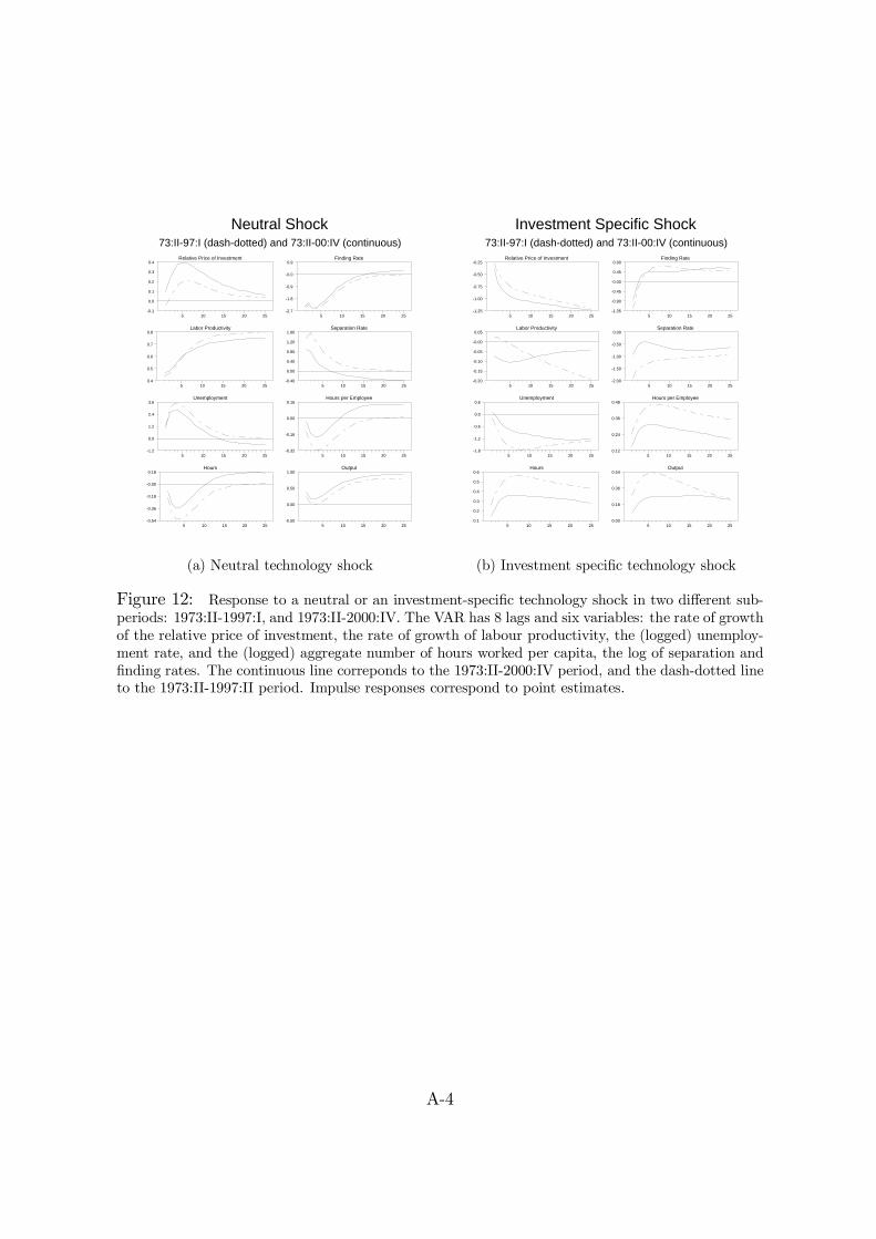
Neutral Shock73:II-97:I (dash-dotted) and 73:II-00:IV (continuous)

Relative Price of Investment

5 10 15 20 25-0.1

0.0

0.1

0.2

0.3

0.4

Labor Productivity

5 10 15 20 250.4

0.5

0.6

0.7

0.8

Unemployment

5 10 15 20 25-1.2

0.0

1.2

2.4

3.6

Hours

5 10 15 20 25-0.54

-0.36

-0.18

-0.00

0.18

Finding Rate

5 10 15 20 25-2.7

-1.8

-0.9

-0.0

0.9

Separation Rate

5 10 15 20 25-0.40

0.00

0.40

0.80

1.20

1.60

Hours per Employee

5 10 15 20 25-0.32

-0.16

0.00

0.16

Output

5 10 15 20 25-0.50

0.00

0.50

1.00

Investment Specific Shock73:II-97:I (dash-dotted) and 73:II-00:IV (continuous)

Relative Price of Investment

5 10 15 20 25-1.25

-1.00

-0.75

-0.50

-0.25

Labor Productivity

5 10 15 20 25-0.20

-0.15

-0.10

-0.05

-0.00

0.05

Unemployment

5 10 15 20 25-1.8

-1.2

-0.6

0.0

0.6

Hours

5 10 15 20 250.1

0.2

0.3

0.4

0.5

0.6

Finding Rate

5 10 15 20 25-1.35

-0.90

-0.45

-0.00

0.45

0.90

Separation Rate

5 10 15 20 25-2.00

-1.50

-1.00

-0.50

0.00

Hours per Employee

5 10 15 20 250.12

0.24

0.36

0.48

Output

5 10 15 20 250.00

0.18

0.36

0.54

(a) Neutral technology shock (b) Investment specific technology shock

Figure 12: Response to a neutral or an investment-specific technology shock in two different sub-periods: 1973:II-1997:I, and 1973:II-2000:IV. The VAR has 8 lags and six variables: the rate of growthof the relative price of investment, the rate of growth of labour productivity, the (logged) unemploy-ment rate, and the (logged) aggregate number of hours worked per capita, the log of separation andfinding rates. The continuous line correponds to the 1973:II-2000:IV period, and the dash-dotted lineto the 1973:II-1997:II period. Impulse responses correspond to point estimates.

A-4

Neutral Shock55:I-00:IV (continuous), 55:I-74:II (dotted), 74:III-97:I (dash-dotted)

Relative Price of Investment

5 10 15 20 25-0.15

-0.10

-0.05

0.00

0.05

0.10

Labor Productivity

5 10 15 20 250.2

0.4

0.6

0.8

1.0

Unemployment

5 10 15 20 25-1.2

0.0

1.2

2.4

3.6

4.8

Hours

5 10 15 20 25-0.54

-0.36

-0.18

-0.00

0.18

Finding Rate

5 10 15 20 25-4.2

-2.8

-1.4

0.0

1.4

Separation Rate

5 10 15 20 25-1.4

-0.7

0.0

0.7

1.4

Hours per Employee

5 10 15 20 25-0.3

-0.2

-0.1

-0.0

Output

5 10 15 20 25-0.25

0.00

0.25

0.50

0.75

1.00

Investment Specific Shock55:I-00:IV (continuous), 55:I-74:II (dotted), 74:III-97:I (dash-dotted)

Relative Price of Investment

5 10 15 20 25-1.35

-0.90

-0.45

-0.00

Labor Productivity

5 10 15 20 25-0.48

-0.36

-0.24

-0.12

0.00

0.12

Unemployment

5 10 15 20 25-1.8

-0.9

0.0

0.9

1.8

Hours

5 10 15 20 25-0.2

0.0

0.2

0.4

0.6

Finding Rate

5 10 15 20 25-1.6

-0.8

0.0

0.8

1.6

Separation Rate

5 10 15 20 25-1.6

-0.8

0.0

0.8

1.6

2.4

Hours per Employee

5 10 15 20 25-0.16

0.00

0.16

0.32

0.48

Output

5 10 15 20 25-0.60

-0.30

0.00

0.30

0.60

(a) Neutral technology shock (b) Investment specific technology shock

Figure 13: Responses to a one-standard deviation shocks in thre different subsamples. The subsam-ples are: 1955:I-2000:IV, 1955:I-1974:II, and 1974:III-1997:I. Each line corresponds to a six variableVAR(8) with the rate of growth of the relative price of investment, the rate of growth of labour pro-ductivity, the (logged) unemployment rate, and the (logged) aggregate number of hours worked percapita, the log of separation and finding rates, estimated over a different sample period.

A-5

Neutral Shock55:I-00:IV (continuous), 55:I-75:IV (dotted), 76:I-97:I (dash-dotted)

Relative Price of Investment

5 10 15 20 25-0.14

0.00

0.14

0.28

Labor Productivity

5 10 15 20 250.18

0.36

0.54

0.72

0.90

Unemployment

5 10 15 20 25-1.8

0.0

1.8

3.6

5.4

Hours

5 10 15 20 25-0.54

-0.36

-0.18

-0.00

0.18

Finding Rate

5 10 15 20 25-4.8

-3.2

-1.6

-0.0

1.6

Separation Rate

5 10 15 20 25-1.6

-0.8

0.0

0.8

1.6

Hours per Employee

5 10 15 20 25-0.27

-0.18

-0.09

-0.00

0.09

Output

5 10 15 20 25-0.25

0.00

0.25

0.50

0.75

1.00

Investment Specific Shock55:I-00:IV (continuous), 55:I-75:IV (dotted), 76:I-97:I (dash-dotted)

Relative Price of Investment

5 10 15 20 25-1.35

-0.90

-0.45

-0.00

Labor Productivity

5 10 15 20 25-0.4

-0.2

0.0

0.2

Unemployment

5 10 15 20 25-3

-2

-1

0

1

Hours

5 10 15 20 25-0.16

0.00

0.16

0.32

0.48

0.64

Finding Rate

5 10 15 20 25-2

-1

0

1

2

Separation Rate

5 10 15 20 25-2.0

-1.5

-1.0

-0.5

0.0

0.5

Hours per Employee

5 10 15 20 25-0.16

0.00

0.16

0.32

0.48

Output

5 10 15 20 25-0.45

0.00

0.45

0.90

(a) Neutral technology shock (b) Investment specific technology shock

Figure 14: Responses to a one-standard deviation shocks in thre different subsamples. The subsam-ples are: 1955:I-2000:IV, 1955:I-1975:IV, and 1976:I-1997:I. Each line corresponds to a six variableVAR(8) with the rate of growth of the relative price of investment, the rate of growth of labour pro-ductivity, the (logged) unemployment rate, and the (logged) aggregate number of hours worked percapita, the log of separation and finding rates, estimated over a different sample period.

A-6

Neutral ShockRelative Price of Investment

5 10 15 20 25-0.08

0.00

0.08

0.16

0.24

0.32

Labor Productivity

5 10 15 20 250.18

0.27

0.36

0.45

0.54

Unemployment

5 10 15 20 25-1

0

1

2

3

Hours

5 10 15 20 25-0.32

-0.24

-0.16

-0.08

0.00

0.08

Finding Rate

5 10 15 20 25-2.7

-1.8

-0.9

-0.0

0.9

Separation Rate

5 10 15 20 25-0.45

0.00

0.45

0.90

1.35

1.80

Hours per Employee

5 10 15 20 25-0.15

-0.10

-0.05

0.00

0.05

0.10

Output

5 10 15 20 25-0.2

0.0

0.2

0.4

0.6

Investment Specific ShockRelative Price of Investment

5 10 15 20 25-0.84

-0.70

-0.56

-0.42

-0.28

-0.14

Labor Productivity

5 10 15 20 25-0.27

-0.18

-0.09

-0.00

0.09

Unemployment

5 10 15 20 25-2

-1

0

1

Hours

5 10 15 20 250.00

0.25

0.50

0.75

Finding Rate

5 10 15 20 25-1.4

-0.7

0.0

0.7

1.4

Separation Rate

5 10 15 20 25-1.60

-1.20

-0.80

-0.40

-0.00

0.40

Hours per Employee

5 10 15 20 250.0

0.2

0.4

0.6

Output

5 10 15 20 25-0.2

0.0

0.2

0.4

0.6

(a) Neutral technology shock (b) Investment specific technology shock

Figure 15: Response to a neutral or an investment-specific technology shock in a nine variables VARwith approximated rates. 1955:I-2000:IV sample with intercept deterministically broken at 1973:II and1997:I. Dotted lines represent the 5% and 95% quantiles of the distribution of the responses simulatedby bootstrapping 500 times the residuals of the VAR. The continuous line corresponds to medianestimate.

A-7

Correlation with Oil prices and FED rate

Neutral shockOil price

-6 -4 -2 0 2 4 6-0.50

-0.25

0.00

0.25

0.50

FED rate

-6 -4 -2 0 2 4 6-0.50

-0.25

0.00

0.25

0.50

Investment-specific shockOil price

-6 -4 -2 0 2 4 6-0.50

-0.25

0.00

0.25

0.50

FED rate

-6 -4 -2 0 2 4 6-0.50

0.00

0.50

1.00

Figure 16: Left column corresponds to neutral technology shocks; right column to investment specifictechnology shocks. The first row plots the correlation of the corresponding technology shock withrelative oil price shocks (i.e. relative to consumption). The second row with Federal fund rate shocks

at different time horizons. The shocks are estimated from the nine variables VAR, approximatedrates, full sample with deterministic dummies. The horizzontal lines correspond to an asymptotic 95percent confidence interval centered around zero.

A-8

Neutral ShockDummy (continuous), Polynomial (dotted), HP (dashed)

Relative Price of Investment

5 10 15 20 250.000

0.040

0.080

0.120

0.160

Labor Productivity

5 10 15 20 250.4

0.6

0.8

1.0

Unemployment

5 10 15 20 250

1

2

3

4

Hours

5 10 15 20 25-0.5

-0.4

-0.3

-0.2

-0.1

-0.0

Finding Rate

5 10 15 20 25-4.2

-2.8

-1.4

0.0

Separation Rate

5 10 15 20 25-0.6

0.0

0.6

1.2

1.8

2.4

Hours per Employee

5 10 15 20 25-0.3

-0.2

-0.1

-0.0

Output

5 10 15 20 25-0.30

0.00

0.30

0.60

0.90

Investment Specific ShockDummy (continuous), Polynomial (dotted), HP (dashed)

Relative Price of Investment

5 10 15 20 25-1.2

-1.0

-0.8

-0.6

-0.4

Labor Productivity

5 10 15 20 25-0.240

-0.200

-0.160

-0.120

-0.080

Unemployment

5 10 15 20 25-1.50

-1.00

-0.50

0.00

0.50

1.00

Hours

5 10 15 20 25-0.14

0.00

0.14

0.28

0.42

Finding Rate

5 10 15 20 25-1.0

-0.5

0.0

0.5

1.0

Separation Rate

5 10 15 20 25-1.80

-1.35

-0.90

-0.45

-0.00

0.45

Hours per Employee

5 10 15 20 25-0.09

0.00

0.09

0.18

0.27

0.36

Output

5 10 15 20 25-0.24

-0.12

0.00

0.12

0.24

0.36

(a) Neutral technology shock (b) Investment specific technology shock

Figure 17: The continous line corresponds to dummy specification, the dotted line to the case wherethe intercept is a 3rd order polynomial in time. The dashed lines are the responses after detrendingthe original series with an Hodrick Prescott filter with smoothing parameter λ = 10000. VAR withapproximated rates, with 8 lags, and six variables. Plotted impulse responses correspond to pointestimates.

A-9

Neutral Shock8-lags (continuous), 4-lags (dotted), 12-lags (dashed)

Relative Price of Investment

5 10 15 20 25-0.030

0.000

0.030

0.060

0.090

Labor Productivity

5 10 15 20 250.4

0.5

0.6

0.7

0.8

0.9

Unemployment

5 10 15 20 250

1

2

3

4

Hours

5 10 15 20 25-0.6

-0.4

-0.2

-0.0

Finding Rate

5 10 15 20 25-4.8

-3.2

-1.6

-0.0

Separation Rate

5 10 15 20 250.0

0.5

1.0

1.5

2.0

Hours per Employee

5 10 15 20 25-0.36

-0.24

-0.12

0.00

Output

5 10 15 20 25-0.30

0.00

0.30

0.60

0.90

Investment Specific Shock8-lags (continuous), 4-lags (dotted), 12-lags (dashed)

Relative Price of Investment

5 10 15 20 25-1.2

-1.0

-0.8

-0.6

-0.4

Labor Productivity

5 10 15 20 25-0.270

-0.225

-0.180

-0.135

-0.090

-0.045

Unemployment

5 10 15 20 25-1.60

-1.20

-0.80

-0.40

-0.00

Hours

5 10 15 20 250.00

0.09

0.18

0.27

0.36

0.45

Finding Rate

5 10 15 20 25-1.5

-1.0

-0.5

0.0

0.5

1.0

Separation Rate

5 10 15 20 25-2.1

-1.4

-0.7

0.0

Hours per Employee

5 10 15 20 250.00

0.12

0.24

0.36

Output

5 10 15 20 25-0.2

0.0

0.2

0.4

(a) Neutral technology shock (b) Investment specific technology shock

Figure 18: Dummy specification with different lags in the VAR: continous line corresponds to 8lags, dotted line to 4 lags, dashed line to 12 lags. VAR with approximated rates, with 8 lags, and sixvariables. Plotted impulse responses correspond to point estimates.

A-10

Neutral ShockLong-run (continuous), Medium-run (dotted)Relative Price of Investment

5 10 15 20 250.000

0.025

0.050

0.075

0.100

Labor Productivity

5 10 15 20 250.4

0.5

0.6

0.7

0.8

0.9

Unemployment

5 10 15 20 250

1

2

3

4

Hours

5 10 15 20 25-0.5

-0.4

-0.3

-0.2

-0.1

-0.0

Finding Rate

5 10 15 20 25-4.2

-2.8

-1.4

0.0

Separation Rate

5 10 15 20 250.0

0.5

1.0

1.5

Hours per Employee

5 10 15 20 25-0.3

-0.2

-0.1

-0.0

Output

5 10 15 20 25-0.30

0.00

0.30

0.60

0.90

Investment Specific ShockLong-run (continuous), Medium-run (dotted)Relative Price of Investment

5 10 15 20 25-1.2

-1.0

-0.8

-0.6

-0.4

Labor Productivity

5 10 15 20 25-0.25

-0.20

-0.15

-0.10

-0.05

Unemployment

5 10 15 20 25-1.50

-1.00

-0.50

0.00

0.50

Hours

5 10 15 20 250.00

0.14

0.28

0.42

Finding Rate

5 10 15 20 25-1.0

-0.5

0.0

0.5

1.0

Separation Rate

5 10 15 20 25-2.0

-1.5

-1.0

-0.5

0.0

Hours per Employee

5 10 15 20 250.00

0.12

0.24

0.36

Output

5 10 15 20 25-0.2

0.0

0.2

0.4

(a) Neutral technology shock (b) Investment specific technology shock

Figure 19: Dummy specification with identifying restrictions imposed at different time horizons:continous line corresponds to long run restriction, dotted line corresponds to the specification whererestrictions are imposed at an horizon of 3 years. VAR with approximated rates, with 8 lags, and sixvariables. Plotted impulse responses correspond to point estimates.

A-11

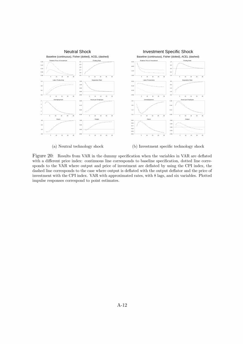
Neutral ShockBaseline (continuous), Fisher (dotted), ACEL (dashed)

Relative Price of Investment

5 10 15 20 250.00

0.05

0.10

0.15

0.20

Labor Productivity

5 10 15 20 250.4

0.6

0.8

1.0

Unemployment

5 10 15 20 250

1

2

3

4

Hours

5 10 15 20 25-0.6

-0.4

-0.2

-0.0

Finding Rate

5 10 15 20 25-4.5

-3.6

-2.7

-1.8

-0.9

-0.0

Separation Rate

5 10 15 20 25-0.50

0.00

0.50

1.00

1.50

Hours per Employee

5 10 15 20 25-0.36

-0.24

-0.12

0.00

Output

5 10 15 20 25-0.50

0.00

0.50

1.00

Investment Specific ShockBaseline (continuous), Fisher (dotted), ACEL (dashed)

Relative Price of Investment

5 10 15 20 25-1.60

-1.20

-0.80

-0.40

Labor Productivity

5 10 15 20 25-0.54

-0.36

-0.18

-0.00

Unemployment

5 10 15 20 25-1.5

-1.0

-0.5

0.0

Hours

5 10 15 20 250.00

0.09

0.18

0.27

0.36

0.45

Finding Rate

5 10 15 20 25-1.0

-0.5

0.0

0.5

1.0

Separation Rate

5 10 15 20 25-2.0

-1.5

-1.0

-0.5

0.0

Hours per Employee

5 10 15 20 250.00

0.12

0.24

0.36

Output

5 10 15 20 25-0.50

-0.25

0.00

0.25

0.50

(a) Neutral technology shock (b) Investment specific technology shock

Figure 20: Results from VAR in the dummy specification when the variables in VAR are deflatedwith a different price index: continuous line corresponds to baseline specification, dotted line corre-sponds to the VAR where output and price of investment are deflated by using the CPI index, thedashed line corresponds to the case where output is deflated with the output deflator and the price ofinvestment with the CPI index. VAR with approximated rates, with 8 lags, and six variables. Plottedimpulse responses correspond to point estimates.

A-12