The interaction between fiscaland macroprudential policy in

emerging countries

Ketkaew KulprapaStudent no. 51-188045

A Thesis Submitted to

Graduate School of Public Policy

University of Tokyo

In Partial Fulfillment of the Requirements for the Degree

Master of Public Policy

December 2, 2019

Contents

Abstract 2

1 Introduction 3

2 Related Literature 8

3 The Model 103.1 Patient Households . . . . . . . . . . . . . . . . . . . . . . . . 113.2 Impatient Households . . . . . . . . . . . . . . . . . . . . . . . 123.3 Entrepreneurs . . . . . . . . . . . . . . . . . . . . . . . . . . . 133.4 Government . . . . . . . . . . . . . . . . . . . . . . . . . . . . 143.5 Market Equilibrium . . . . . . . . . . . . . . . . . . . . . . . . 153.6 Shock and Policy rule . . . . . . . . . . . . . . . . . . . . . . . 17

4 Numerical Experiment 174.1 The effect of fiscal policy shock without macroprudential pol-

icy rules . . . . . . . . . . . . . . . . . . . . . . . . . . . . . . 184.2 The effect of fiscal policy shock with macroprudential policy

rules . . . . . . . . . . . . . . . . . . . . . . . . . . . . . . . . 20

5 Welfare Analysis 24

6 Conclusion 28

7 Appendix 29

References 32

1

Abstract

A continuously increasing credit growth in these recent decadesurges emerging countries to pay more attention on financial stabilitybesides economic growth. According to some academic literature andcountries’ examples, one of the factors that accelerate credit growth isfiscal policy. However, fiscal policy is an important economic stimulustool that every emerging country needs and cannot refrain from usingit. This paper focuses on the interaction between fiscal and macropru-dential policy from the financial stability viewpoint. It, first, investi-gates the negative effect of fiscal policy on financial stability in emerg-ing countries. Next, it examines whether macroprudential policy canmitigate the negative effect from fiscal policy or not. Finally, the paperproposes some policy suggestions that help emerging countries main-tain financial stability without restricting the implementation of fiscalpolicy. The paper is a theoretical study and uses DSGE frameworkin the analysis. Three main results are found. First, fiscal policy caninduce financial instability through the credit market. Second, macro-prudential policy can help stabilizing the volatilities in the economyincluding households and corporates credit. Lastly, implementing thepolicy combination between fiscal and macroprudential policy can en-able emerging countries to achieve financial stability besides economicgrowth, and it also improves the social welfare.

2

1 Introduction

In these recent decades, emerging countries have experienced a continuouslyincreasing economic and credit growth. The world GDP share of emergingcountries has been increasing since 1990s and finally exceeded the share ofdeveloped countries in 2007. In 2018, the world GDP share of emergingand developing countries is 59.24%. One of the factors that contributes toemerging countries’ economic growth is the implementation of fiscal policiessuch as public spending and tax policy. Along with the economic growth,emerging countries are also facing an increasing credit growth. Especially,corporate credit contributes the most to the overall credit growth in everycountry. The increasing credit growth can be either a good or a bad situation.In good case, it implies the development of the country. We can observe apositive correlation between economic growth and credit growth in emergingcountries. Economic and credit growth has a positive influence on each other(Townsend and Ueda (2010), Garcia et al. (2015)). However, at the sametime, credit growth is an index used to measure financial instability, and itis the best predictor of financial crises (Freixas et al. (2015)).

Many international institutions and central banks in emerging countriesstart to be aware of the increasing credit growth issue. For example, Bank ofThailand (BOT) 2017 financial report states that loans to corporate, espe-cially to small and medium enterprises (SMEs), account the biggest share ofthe total loan in Thailand. However, loans to SMEs are likely to become thenon-performing loans (NPL). It is difficult to restrict the amount of loans toSMEs because SMEs performances account a large part of Thailand GDP. In2017, 42.4% of Thailand GDP comes from SMEs. Therefore, BOT insteadmonitors the loan quality in order to control NPL ratio. Another example isChina. Chen and Kang (2018) explains that China has been experiencing arapid credit growth since 2008 (after the Global Financial Crisis). This creditgrowth has supported China economy, but many international institutionsbelieve that this credit growth is not sustainable. Most of the credit goesto industrial and service sectors, but it is ineffectively used. The relianceon infrastructure investment is also another factor that accelerates creditgrowth. A rapid increase in debt raises the concerns about financial stabil-ity in China. Emerging countries are more exposed to domestic and foreignshocks than developed countries. When bad situations happen, for example,currency depreciation, foreign interest rate cut, or changes in demand, it isdifficult to repay the high level of debt. As a response to the increasing creditgrowth in emerging countries, AMRO (2018) suggests that emerging coun-tries’ policymakers should prioritize financial stability over economic growthin the near future. In addition, the combination of fiscal, monetary, and

3

macroprudential policy should be well organized depending on the currentbusiness and credit cycle of each country. One cannot deny that besides eco-nomic growth, financial stability is an upcoming issue that policymakers inemerging countries should consider.

This paper aims to find a policy solution that can maintain financial sta-bility without restricting the economic growth promoting policy, and helpsemerging countries achieve a sustainable development. It focuses on the in-teraction between fiscal and macroprudential policy because the objective offiscal policy is economic growth, and the objective of macroprudential pol-icy is financial stability. Previous studies about financial policies focus onmacroprudential policy itself or its interaction with monetary policy. Thestudy about fiscal and macroprudential policy is relatively scare. There ex-ist some empirical studies that show the negative effect of fiscal policy onfinancial stability (Afonso & Sousa (2012), Hodula (2018)). Some confirmthat macroprudential policy, tightening LTV rate, can cool down the creditgrowth (Alpanda & Zubairy (2017), Erlend & Heedon (2016)). As far as Iknow, the theoretical studies about fiscal and macroprudential policy definefiscal policy as tax system such as mortgage tax deduction regime. Thispaper is new to the extent that it is a theoretical paper that defines fiscalpolicy as government spending. The paper also explains the mechanism thatfiscal policy negatively affects financial stability and the policy solution tothis problem. I hope the implications from the results of this paper willcontribute to the limited study about fiscal and macroprudential policy inemerging countries and help the policymakers figure out the way to maintainfinancial stability and achieve economic growth at the same time.

We can see the example of government spending affecting credit growthin the real world. Thailand, which is a trade partner of many developedcountries and attracts many foreign investors, is carrying out a train con-struction project supported by the government. The government spendsa huge amount of expenditure on the construction and operation. As theconstruction proceeds, the demand for land and houses, mainly condomini-ums, along the railways increases because people expect a higher value of thecondominiums. Same as land and houses, people use condominiums as collat-eral. An increase in condominium price allows people to borrow more. As aconsequence, household credit of Thailand increases. At the same time, con-struction firms borrow and build a massive number of condominiums to meetthe demand. However, the supply seems to be too much and has low quality.Now, there are many condominiums left unsold and many construction plansare called off. The price of condominium falls and creates a serious situationfor both households and firms. Households who carry a large amount of debthave lower ability to repay because of the fall in asset value. Firms also face

4

the difficulty to repay the debt because they cannot sale the condominiums.As a result, the non-performing loans of Thailand increases and becomes aserious issue for BOT. From Thailand case, we can conclude that an increasein government expenditure on infrastructure can increase household and cor-porate loans. With a bad situation, the loans can turn to the non-performingloans, which accelerate the fragility in credit market and financial system.For empirical evidence, Afonso & Sousa (2012) confirms that government ex-penditure can increase house price. In addition, according to the literatureabout credit friction, a rise in house price can be interpreted as an increasein collateral value, which finally increases the amount of credit.

Even though government spending on infrastructure has a side effect onfinancial stability, it is still an important fiscal policy tool that every emerg-ing country needs to promote the economic growth. Infrastructure invest-ment has been an economic stimulus tool since the beginning of the GlobalFinancial Crisis. Even now, Infrastructure demand in emerging countries, es-pecially the demand for transportation infrastructure, continues to increase.The infrastructure spending, mostly supported by the government, also hasan upward trend. According to UBS (2018), emerging countries’ infrastruc-ture spending share will become two-third of the world in 2025. Infrastruc-ture can increase not only the output and productivity of the country, butit also attracts foreign businesses. Many developed countries’ multinationalcompanies suggest that the current infrastructure in emerging countries arestill insufficient, which lessen their incentives to start the businesses despitethe low labor cost. Emerging countries’ governments are aware of this insight.Therefore, they tend to launch many infrastructure construction projectsand are likely to ignore the side effects such as fiscal deficit and rapid creditgrowth.

To maintain the stability in credit market and financial system, macro-prudential policy is needed. Macroprudential policy has financial stability asa prior objective, while fiscal policy’s target is to promote economic growth.When there are some trade-offs between economic growth and financial sta-bility, there is no guarantee that the fiscal policymakers will take financialstability into account. In addition, fiscal policy, especially in emerging coun-try, is influenced by some political factors and may not be optimally used.Dumicic (2019) claims that the optimal fiscal policy is difficult to achievedue to election cycle. Hence, we need another policy that has an objective tocontain the risks and stabilize the financial system. Macroprudential policyis the policy that aims to achieve financial stability and has gathered theinterest since the Global Financial Crisis. Many emerging countries have al-ready introduced macroprudential policy. According to Cerutti et al. (2017),the use of macroprudential policy in emerging country is the highest among

5

other country groups, but the studies about its effects and the interactionwith other policies is still limited.

Some emerging countries have succeeded in curbing financial instabilityby using macroprudential policy. Turkey has faced a rapid credit growthsince the early 2000s, it finally experiences the highest credit growth amongemerging countries during 2010 to 2012 (Garcia et al. (2015)). As a conse-quence, Turkey has implemented a sequence of macroprudential policies since2011. Turkey establishes Financial Stability Committee (FSC) as a formalauthority that is responsible for macroprudential policy. The FSC uses var-ious packages of policies to contain credit growth and household debt. Con-cretely, the FSC puts higher risk weights for consumer loan, higher minimumpayments for credit card debt, and introduces loan-to-value (LTV) caps forhousing loans. After implementing the policies, consumer loans vividly de-crease. However, corporate loans do not change much because the introducedpolicy tools target only household indebtness. To conclude, macroprudentialpolicy helps Turkey contain the risks in credit market. A well study aboutthe effect of each policy tool and choosing the right policy at the right timeis important.

This paper explores the effect of fiscal policy and macroprudential policyon emerging market economy, focusing especially on the financial stabilityviewpoint, and provides some policy suggestions. In this paper, fiscal pol-icy refers to government spending on infrastructure, macroprudential policyrefers to loan-to-value (LTV) ratio, and financial instability refers to the in-crease in household and corporate credit-to-GDP from steady state level.The paper is a theoretical study and uses DSGE framework. It, first, ex-amines whether fiscal policy can induce financial instability or not. Next,it investigates whether macroprudential policy can help mitigate the nega-tive effect of fiscal policy. Finally, the paper does the welfare analysis of thepolicies in order to find out what kind of policy combination benefits theeconomy.

In order to study the above 3 research questions, I construct a modelthat has infrastructure as a factor of production and the credit marketwhere agents in the economy can directly lend and borrow the money sub-ject to some borrowing constraints. There is no bank in this model. Thelender is patient households, and the borrowers are impatient householdsand entrepreneurs. Household credit is the amount of borrowing impatienthouseholds borrow from patient households. Corporate credit is the amountof borrowing entrepreneurs borrow from patient households. I use DSGEframework to capture the effect of fiscal policy shock, which is a positiveinfrastructure spending shock. I call the situation when there exists a fiscalpolicy shock, but the LTV rates are fixed at a certain value as a benchmark

6

case. After that, I study the effect of macroprudential policy by adding themacroprudential policy rules to the simulation and compare the result withthe benchmark case. Under macroprudential policy rules, the LTV rates areallowed to change responding to the changes in household and corporate bor-rowings. Since there are 2 kinds of credit (household and corporate), thereare 2 kinds of macroprudential policy tools; household LTV rate and cor-porate LTV rate. Each tool targets different agents. Lastly, I compute thesteady state value of the social welfare and the welfare of each agent. ThenI observe how the values change when I tighten the LTV rates. With thismethod, I can capture the welfare effect of macroprudential policy.

Three main findings are found. First, fiscal policy can induce financialinstability. An increase in government spending on infrastructure increasesboth household and corporate credit. Second, macroprudential policy canhelp stabilizing the volatilities of the variables in the economy includinghousehold and corporate credit. The introduction of household LTV raterule decreases the volatility of impatient households’ borrowing. CorporateLTV rate rule has a wider effect. It decreases not only the volatility of en-trepreneurs’ borrowing but also the volatilities of all variables in the economy.Lastly, using fiscal and macroprudential policy together can improve the so-cial welfare, which is defined as a weighted average welfare of the agents inthe economy. However, there are welfare trade-offs between agents.

This paper is most related to Iacoviello (2005) to the extent that it modelsthe economy with credit market, and the agents are subject to the borrow-ing constraints. The difference is that this paper does not consider inflationbecause it wants to focus on fiscal and macroprudential policy. Iacoviello(2005), on the other hand, focuses on monetary policy, and incorporate in-flation and nominal interest rate into the model. This paper also related toMendicino and Punzi (2014) in the sense that it introduces LTV rate as themacroprudential policy tool. However, the paper defines financial instabilityas the fragility in domestic credit market, while Mendizino and Punzi (2014)takes current account as the financial instability index.

In the next section, I introduce some related literature to prepare somebackground information relevant to this study and support the argumentsin this paper. Section 3 presents the model. Section 4 discusses about theparameters used in the numerical experiment and shows the results. Section5 analyzes the welfare effect of the policies introduced in the model. Section6 concludes.

7

2 Related Literature

International institutions and central banks in emerging countries start toworry about an increasing credit growth because credit growth is a sign offinancial crises and can cause some risks in financial system. According toFreixas et al. (2015), a rapid credit growth, or in other words, credit boomin emerging markets increases the interest rate, which attracts the foreigncapital. The inflow of foreign capital, then, accelerates the domestic creditgrowth and asset bubbles. The situation can develop to a systemic risk andthreaten the stability of the financial system. The rises in credit and assetprice, as we can see in many emerging countries, are signs of credit boomsand asset price bubbles, and sequentially the crises. Monitoring credit growthis one way to maintain financial stability and prevent the country from thecrises. (Jorda et al. (2011), (2013))

There are several factors that can accelerate the credit cycle in an un-healthy way, for example, monetary policy and fiscal policy. Claessens (2014)summarizes 6 channels that monetary policy can affect financial stability.Among these 6 channels, there are both positive and negative relationshipbetween interest rate and financial stability. A rise in interest rate may im-prove financial stability in some channels but deteriorate in the others. Thepaper also proposes some macroprudential policy tools that can reduce theside effects of monetary policy and suggests that the combination betweenthese two policies can enhance the economy.

Fiscal policy such as tax system can increase the risk in credit cycle.According to IMF (2013), corporate tax system can create debt bias. Thesystem makes the corporates choose debt rather than equity as a fundingmethod. Since debt interest payment is deductible in the taxable profit cal-culation, while equity dividend is not, the corporates prefer to issue debt andpay more interest, so that they can pay less corporate tax. This results in ahigh level of corporate credit, which is a source of fragility in financial system.In addition, housing-related tax policy such as mortgage interest deductioncan increase household debt and lead to output losses of the economy (Al-panda & Zubairy (2016)). In order to decrease household credit, tighteningLTV rate and reducing mortgage interest deduction are the effective and lesscostly tools (Alpanda & Zubairy (2017)).

Government expenditure, another fiscal policy tool, also affects financialstability. According to the empirical work of Hodula (2018), an increasein government expenditure raises the demand for credit. The paper arguesthat the credit increases through the housing market because house price hasan upward response to the government expenditure shock. Because peopleuse houses as collateral, the credit demand leads to an increase in housing

8

demand and, hence, the rise in house price.A tool that can stabilize financial system and has gained attentions af-

ter Asian financial crisis is macroprudential policy. Some empirical studiesshare the same view that borrower-based macroprudential policy tools suchas LTV rate can significantly reduce household credit growth and improvethe social welfare (Morgan et al. (2019), Cerutti et al. (2015), Kuttner andShim (2013)). Theoretical study has also been done. Garbers and Liu (2018)generates a model of small open economy to investigate the effect of macro-prudential policy on the economy when there is a positive foreign interestrate shock, which decreases the supply of foreign funds. They use 2 macro-prudential policy tools, namely caps on LTV rate and capital requirement.They conclude that both macroprudential policy tools benefit the stabilityof financial sector and the economy.

Another strand of literature about macroprudential policy is the studyabout its interaction with other policies. Most of the studies mainly focuson the interaction between monetary and macroprudential policy. Erlend &Heedon (2016) empirically tests whether the effect of macroprudential policyis enhanced when altogether used with monetary policy, but the result is in-significant. For theoretical study, Aoki et al. (2018) constructs a small openeconomy model with international financial market to explore the effect ofmacroprudential policy when there is an external shock and its interactionwith monetary policy. They define the external financial shock as a positiveforeign interest rate shock, which leads to local currency depreciation and,then, results in high inflation and high nominal value of foreign debt. Themacroprudential policy tool used in their paper is tax on foreign currency.The result states that the combination of both monetary and macropruden-tial policy is effective to mitigate the effect of foreign shock, while usingmonetary policy solely decreases the welfare. Mendicino and Punzi (2014)builds a 2-country DSGE model with foreign and domestic shocks. For ex-ample, risk premium shock and housing preference shock are incorporated inthe model. They investigate the shock transmission toward house price andhousehold credit. Then, they examine the effect of macroprudential policy,defined as LTV rate, and its interaction with monetary policy. The resultsays that using 2 policies altogether can reduce macroeconomic and financialfluctuation and is Pareto-improving.

There is also a literature that studies the interaction between fiscal policyand macroprudential policy. Carvalho and Castro (2017) constructs a modelto examine the effect of macroprudential policy and the optimal combinationof macroprudential, fiscal, and monetary policy in Brazilian economy whenthere are external shocks. One of their results suggests that fiscal policy iseffective if the implementation of macroprudential policy is allowed.

9

3 The Model

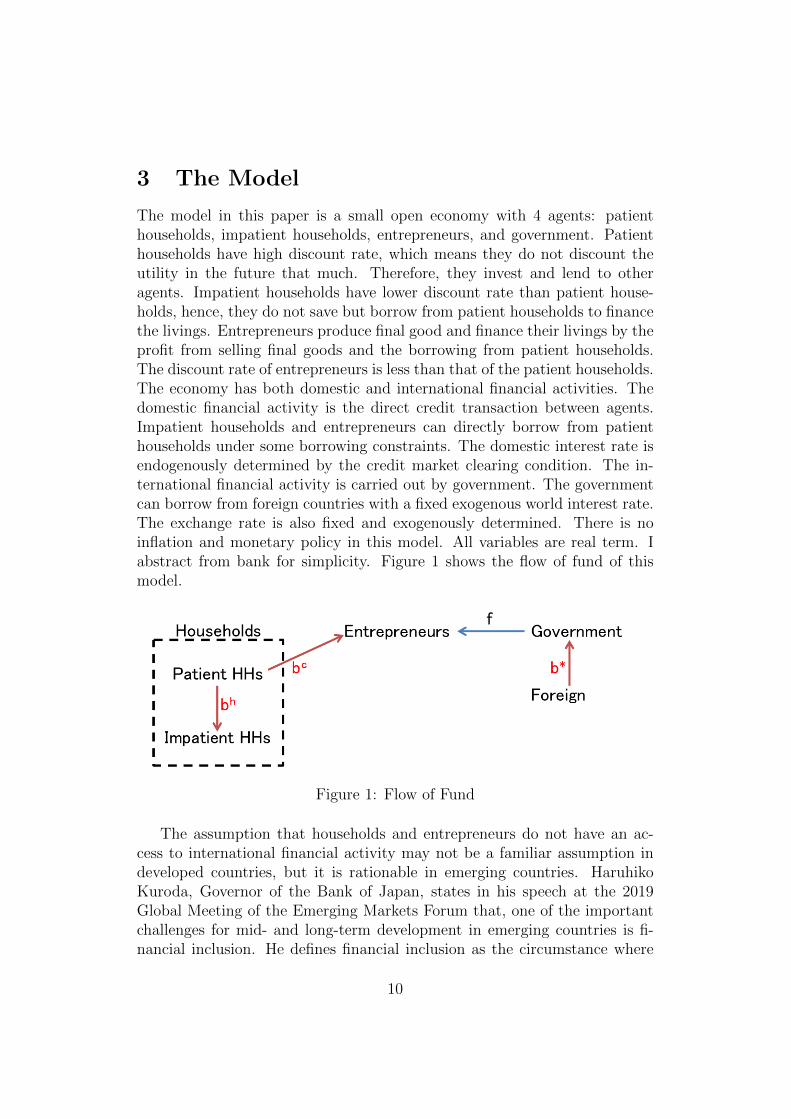
The model in this paper is a small open economy with 4 agents: patienthouseholds, impatient households, entrepreneurs, and government. Patienthouseholds have high discount rate, which means they do not discount theutility in the future that much. Therefore, they invest and lend to otheragents. Impatient households have lower discount rate than patient house-holds, hence, they do not save but borrow from patient households to financethe livings. Entrepreneurs produce final good and finance their livings by theprofit from selling final goods and the borrowing from patient households.The discount rate of entrepreneurs is less than that of the patient households.The economy has both domestic and international financial activities. Thedomestic financial activity is the direct credit transaction between agents.Impatient households and entrepreneurs can directly borrow from patienthouseholds under some borrowing constraints. The domestic interest rate isendogenously determined by the credit market clearing condition. The in-ternational financial activity is carried out by government. The governmentcan borrow from foreign countries with a fixed exogenous world interest rate.The exchange rate is also fixed and exogenously determined. There is noinflation and monetary policy in this model. All variables are real term. Iabstract from bank for simplicity. Figure 1 shows the flow of fund of thismodel.

Figure 1: Flow of Fund

The assumption that households and entrepreneurs do not have an ac-cess to international financial activity may not be a familiar assumption indeveloped countries, but it is rationable in emerging countries. HaruhikoKuroda, Governor of the Bank of Japan, states in his speech at the 2019Global Meeting of the Emerging Markets Forum that, one of the importantchallenges for mid- and long-term development in emerging countries is fi-nancial inclusion. He defines financial inclusion as the circumstance where

10

”households and businesses have access to appropriate financial services andare able to use them effectively”. By promoting financial inclusion, it canhelp improve poverty, inequality, and also support economic growth. How-ever, according to the World Bank, about 40% of the adult population inemerging countries does not have a bank account. Based on his speech, onemay conclude that the access to financial activities even the domestic oneis still limited in emerging countries. Therefore, the access to internationalfinancial activities, such as foreign borrowing, is a difficult issue.

The assumption that government cannot borrow from households is alsoa doubtful assumption in developed countries, but it is a reasonable one inemerging countries. In developed countries such as Japan, the governmentborrows the money by issuing government bond, and the government bondholders are the households in that country. On the other hand, in emerg-ing countries, the domestic agents have little opportunity to buy governmentbond due to the lack of financial inclusion mentioned in the previous para-graph. In order to buy government bond, an agent needs a bank account oran access to a brokerage. Considering the current level of financial inclusionin emerging countries, issuing government bond toward the domestic marketis still difficult. In addition, the data from IMF says that in most emergingcountries, a large proportion of government debt is held by foreign agentssuch as foreign official sector, foreign bank, and foreign non-bank. This datasupports the argument that domestic agents in emerging countries do nothold government bond. Hence, the assumption that there is no governmentbond in this model is a justified assumption for emerging countries.

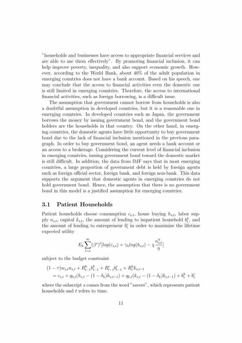
3.1 Patient Households

Patient households choose consumption cs,t, house buying hs,t, labor sup-ply ns,t, capital ks,t, the amount of lending to impatient household bht , andthe amount of lending to entrepreneur bct in order to maximize the lifetimeexpected utility

E0

∞∑t=o

(βs)t[log(cs,t) + γhlog(hs,t)− χnηs,tη

]

subject to the budget constraint

(1− τ)ws,tns,t +Rht−1b

ht−1 +Rc

t−1bct−1 +Rk

t ks,t−1

= cs,t + qh,t(hs,t − (1− δh)hs,t−1) + qk,t(ks,t − (1− δk)ks,t−1) + bht + bct

where the subscript s comes from the word ”savers”, which represents patienthouseholds and t refers to time.

11

βs is patient households’ discount rate, γh is house preference, χ is laborpreference, η is labor inverse, τ is labor income tax rate, ws,t is patienthouseholds’ wage, Rh

t−1 is the return from lending to impatient households,Rct−1 is the return from lending to entrepreneurs, Rk

t−1 is the return fromcapital investment, δh is the depreciation rate of house, δk is the depreciationrate of capital, qh,t is house price, and qk,t is capital price. House price andcapital price are endogenously determined by the house and capital marketconditions, respectively.

Patient households earn income from after-taxed income, return fromlending to impatient households and entrepreneurs, and return from capital.Patient households, then, spend the income on consumption, house buying,capital investment, and lending to impatient households and entrepreneurs.

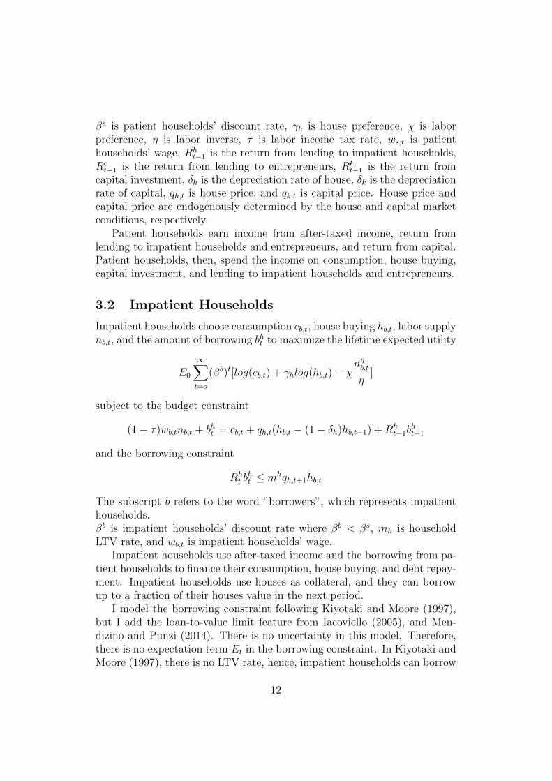
3.2 Impatient Households

Impatient households choose consumption cb,t, house buying hb,t, labor supplynb,t, and the amount of borrowing bht to maximize the lifetime expected utility

E0

∞∑t=o

(βb)t[log(cb,t) + γhlog(hb,t)− χnηb,tη

]

subject to the budget constraint

(1− τ)wb,tnb,t + bht = cb,t + qh,t(hb,t − (1− δh)hb,t−1) +Rht−1b

ht−1

and the borrowing constraint

Rht bht ≤ mhqh,t+1hb,t

The subscript b refers to the word ”borrowers”, which represents impatienthouseholds.βb is impatient households’ discount rate where βb < βs, mh is householdLTV rate, and wb,t is impatient households’ wage.

Impatient households use after-taxed income and the borrowing from pa-tient households to finance their consumption, house buying, and debt repay-ment. Impatient households use houses as collateral, and they can borrowup to a fraction of their houses value in the next period.

I model the borrowing constraint following Kiyotaki and Moore (1997),but I add the loan-to-value limit feature from Iacoviello (2005), and Men-dizino and Punzi (2014). There is no uncertainty in this model. Therefore,there is no expectation term Et in the borrowing constraint. In Kiyotaki andMoore (1997), there is no LTV rate, hence, impatient households can borrow

12

up to a level that the repayment does not exceed the market value of thehouses in the next period. With mh (0 < mh < 1) in the borrowing con-straint, impatient households can borrow only a fraction of their collateralvalue. In reality, central banks use LTV rate as a macroprudential policytool to control the amount of borrowing. At steady state, the borrowingconstraint is always binding. 1

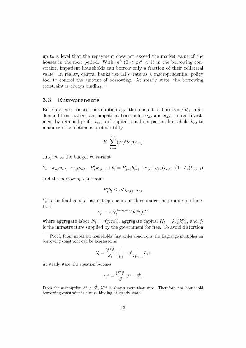
3.3 Entrepreneurs

Entrepreneurs choose consumption cc,t, the amount of borrowing bct , labordemand from patient and impatient households ns,t and nb,t, capital invest-ment by retained profit kc,t, and capital rent from patient household ks,t tomaximize the lifetime expected utility

E0

∞∑t=o

(βc)tlog(cc,t)

subject to the budget constraint

Yt−ws,tns,t−wb,tnb,t−Rkt ks,t−1+bct = Rc

t−1bct−1+cc,t+qk,t(kc,t−(1−δk)kc,t−1)

and the borrowing constraint

Rctbct ≤ mcqk,t+1kc,t

Yt is the final goods that entrepreneurs produce under the production func-tion

Yt = AN1−αk−αft Kαk

t fαft

where aggregate labor Nt = n0.5s,tn

0.5b,t , aggregate capital Kt = k0.5s,t k

0.5c,t , and ft

is the infrastructure supplied by the government for free. To avoid distortion

1Proof: From impatient households’ first order conditions, the Lagrange multiplier onborrowing constraint can be expressed as

λ′t =(βb)t

Rt{ 1

cb,t− βb 1

cb,t+1Rt}

At steady state, the equation becomes

λ′ss =(βb)t

cssb{βs − βb}

From the assumption βs > βb, λ′ss is always more than zero. Therefore, the householdborrowing constraint is always binding at steady state.

13

within labor and capital market, and for simplicity, I assume the share ofpatient and impatient households labor, and also the share of entrepreneursowned-capital and rent capital are 0.5 equally.The subscript c comes from the word ”corporates”, which represents en-trepreneurs. βc is entrepreneurs’ discount rate where βc < βs, and mc iscorporate LTV rate.

Entrepreneurs use the profit from selling final goods and the borrowingfrom patient households to repay the debt, consume, and invest in capi-tal. The borrowing constraint is the same as impatient households but en-trepreneurs use owned-capital instead of houses as collateral. Same as impa-tient households, the entrepreneurs borrowing constraint is always bindingat steady state. 2

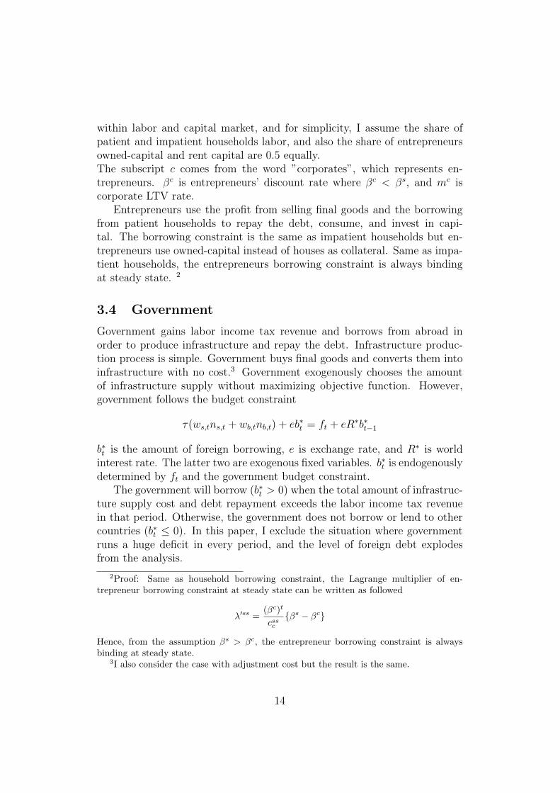
3.4 Government

Government gains labor income tax revenue and borrows from abroad inorder to produce infrastructure and repay the debt. Infrastructure produc-tion process is simple. Government buys final goods and converts them intoinfrastructure with no cost.3 Government exogenously chooses the amountof infrastructure supply without maximizing objective function. However,government follows the budget constraint

τ(ws,tns,t + wb,tnb,t) + eb∗t = ft + eR∗b∗t−1

b∗t is the amount of foreign borrowing, e is exchange rate, and R∗ is worldinterest rate. The latter two are exogenous fixed variables. b∗t is endogenouslydetermined by ft and the government budget constraint.

The government will borrow (b∗t > 0) when the total amount of infrastruc-ture supply cost and debt repayment exceeds the labor income tax revenuein that period. Otherwise, the government does not borrow or lend to othercountries (b∗t ≤ 0). In this paper, I exclude the situation where governmentruns a huge deficit in every period, and the level of foreign debt explodesfrom the analysis.

2Proof: Same as household borrowing constraint, the Lagrange multiplier of en-trepreneur borrowing constraint at steady state can be written as followed

λ′ss =(βc)t

cssc{βs − βc}

Hence, from the assumption βs > βc, the entrepreneur borrowing constraint is alwaysbinding at steady state.

3I also consider the case with adjustment cost but the result is the same.

14

The supply of infrastructure in this model is a fiscal policy tool, by whichthe government can directly control output and indirectly control the agents’income. I model the change in infrastructure supply as a fiscal policy shockin the economy. Details about the fiscal policy shock will be explained insection 3.6.

3.5 Market Equilibrium

The final goods are used for consumption, infrastructure production, andexport. Export is the amount of period t− 1 foreign debt repayment minusthe amount of new foreign borrowing in period t. The good market clearingcondition is as follows.

Yt = cs,t + cb,t + cc,t + ft + e(R∗b∗t−1 − b∗t )

Following Iacoviello (2005), the total amount of house and capital is fixed.Hence, the house and capital market clearing conditions are

hs,t + hb,t = H

ks,t + kc,t = K

H and K are, respectively, the total amount of house and capital.I derive the first order conditions of each agent and substitute the la-

bor market clearing conditions into other equations to get the reduced formversion of the model. The competitive equilibrium is a sequence of 11 endoge-nous quantity variables {cs,t, hs,t, cb,t, hb,t, cc,t, Yt, bht , bct , b∗t , ks,t, kc,t}, 4 endoge-nous price variables {qh,t, qk,t, Rt, R

kt }, and 14 parameters {βs, βb, βc, χ, η, γh,mh,mc, δh, δk, αk,

αf , e, R∗} which satisfies the following 15 equations.

1

cs,t= βs

1

cs,t+1

Rt (1)

where Rt ≡ Rht = Rc

t

qh,tcs,t

=γh

hs,t+ βs

qh,t+1

cs,t+1

(1− δh) (2)

Rt =1

qk,tEt[R

kt+1 + qk,t+1(1− δk)] (3)

cbt+qh,t(hb,t−(1−δh)hb,t−1)+Rt−1bht−1 = (1−τ)(0.5)(1−αk−αf )Yt+bht (4)

15

Rtbht = mhqh,t+1hb,t (5)

qh,tcb,t

=γh

hb,t+ βb

qh,t+1

cb,t+1

(1− δh) +mhqh,t+1

Rt

{ 1

cb,t− βb Rt

cb,t+1

} (6)

Yt = At[(ns,t)0.5(nb,t)

0.5]1−αk−αf [(kc,t−1)0.5(ks,t−1)

0.5]αkfαft (7)

where ni,t = { Ytci.t

0.5(1−αk−αf )(1−τ)χ

}1η i = s, b

Rctbct = mcqk,t+1kc,t (8)

βc1

cc,t+1

{(0.5)αkYt+1

kc,t+qk,t+1(1−δk)}+

1

Rt

(1

cc,t−βc Rt

cc,t+1

)mcqk,t+1 =qk,tcc,t

(9)

(0.5)αkYt+1

ks,t= Rk

t+1 (10)

Rct−1b

ct−1+cc,t = Yt−ws,tns,t−wb,tnb,t−qk,t(kc,t−(1−δk)kc,t−1)−Rk

t ks,t−1+bct(11)

τ(ws,tns,t + wb,tnb,t) + eb∗t = ft + eR∗b∗t−1 (12)

where ws,tns,t = wb,tnb,t = 0.5(1− αk − αf )Yt

Yt = cs,t + cb,t + cc,t + ft + e(R∗b∗t−1 − b∗t ) (13)

hs,t + hb,t = H (14)

ks,t + kc,t = K (15)

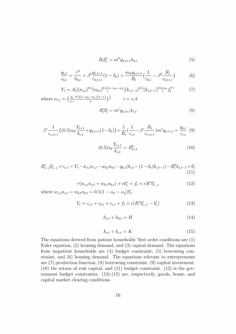
The equations derived from patient households’ first order conditions are (1)Euler equation, (2) housing demand, and (3) capital demand. The equationsfrom impatient households are (4) budget constraint, (5) borrowing con-straint, and (6) housing demand. The equations relevant to entrepreneursare (7) production function, (8) borrowing constraint, (9) capital investment,(10) the return of rent capital, and (11) budget constraint. (12) is the gov-ernment budget constraints. (13)-(15) are, respectively, goods, house, andcapital market clearing conditions.

16

3.6 Shock and Policy rule

The shock in this model is a fiscal policy shock that follows an AR(1) processwith coefficient 0.9. A positive fiscal shock occurs when the governmentarbitrarily increases the supply of infrastructure for some reasons. In reality,the governments in emerging countries usually use fiscal policy as a tool togain the approval rating from the people, especially before the election.

The macroprudential policy rules to stabilize the credit market are asfollows.

mht = mhss(

bhtbhss

)−φh

mct = mcss(

bctbcss

)−φc

where superscript ss means the steady state value of each variable. φh andφc are the parameters that show how strongly the policymakers will responseto the volatility in household and entrepreneur borrowing respectively. TheLTV rates are tightened when the amount of borrowing deviate from thesteady state value. In the next section, I report the simulation result of thepositive fiscal policy shock.

4 Numerical Experiment

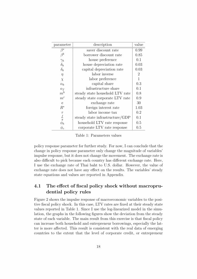
Table 1 reports the parameter values. Most of them follow the previous stud-ies and the values are standard in macroeconomics. I set the steady statevalue of household and entrepreneur LTV rates based on the actual ratesdata of emerging countries. Between 2 types of LTV rate, corporate LTVrate is relatively higher than household LTV rate because entrepreneurs areone of the main sources of economy growth and many emerging countries’governments have the policies that encourage entrepreneurs to produce. Inaddition to high LTV rate, entrepreneurs also have other credit privilegessuch as loose borrowing conditions and an extension of debt repayment. Thevalue of infrastructure share in this model is lower than the value in pre-vious literature because the previous literature uses the data of developedcountry in the computation. However, according to UNECE (2016), the con-tribution of infrastructure on output is different because of the deficiency inpublic investment. Calderon et al. (2014) uses the data of 88 industrial anddeveloping countries to estimate the contribution of infrastructure on out-put. They conclude that 10% increase in infrastructure may raise output perworker by 0.7% to 1%. Macroprudential policy response is difficult to choosebecause of the lack of literature about this topic. I leave the realistic value of

17

parameter description value

βs saver discount rate 0.99βb borrower discount rate 0.85γh house preference 0.1δh house depreciation rate 0.03δk capital depreciation rate 0.03η labor inverse 2χ labor preference 1αk capital share 0.3αf infrastructure share 0.1mh steady state household LTV rate 0.8mc steady state corporate LTV rate 0.9e exchange rate 30R∗ foreign interest rate 1.03τ labor income tax 0.2fy

steady state infrastructure/GDP 0.1

φh household LTV rate response 0.5φc corporate LTV rate response 0.5

Table 1: Parameters values

policy response parameter for further study. For now, I can conclude that thechange in policy response parameter only change the magnitude of variables’impulse response, but it does not change the movement. The exchange rate isalso difficult to pick because each country has different exchange rate. Here,I use the exchange rate of Thai baht to U.S. dollar. However, the value ofexchange rate does not have any effect on the results. The variables’ steadystate equations and values are reported in Appendix.

4.1 The effect of fiscal policy shock without macropru-dential policy rules

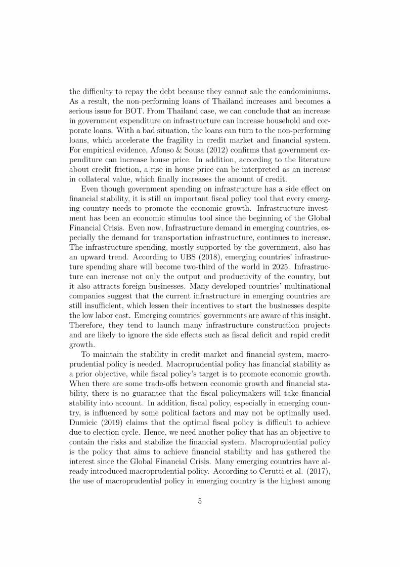
Figure 2 shows the impulse response of macroeconomic variables to the posi-tive fiscal policy shock. In this case, LTV rates are fixed at their steady statevalues reported in Table 1. Since I use the log-linearized model in the simu-lation, the graphs in the following figures show the deviation from the steadystate of each variable. The main result from this exercise is that fiscal policycan increase both household and entrepreneur borrowings, especially the lat-ter is more affected. This result is consistent with the real data of emergingcountries to the extent that the level of corporate credit, or entrepreneur

18

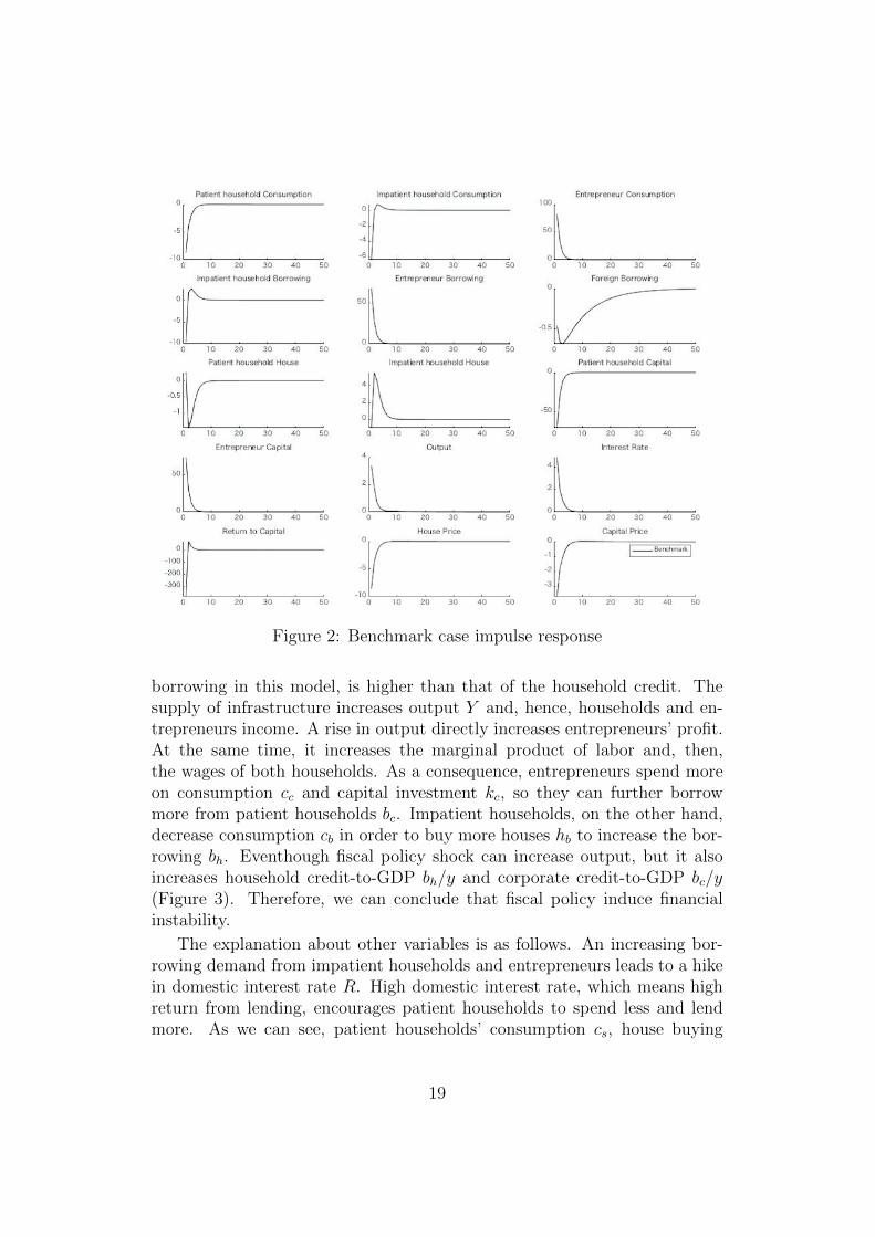
Figure 2: Benchmark case impulse response

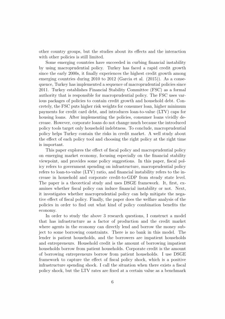
borrowing in this model, is higher than that of the household credit. Thesupply of infrastructure increases output Y and, hence, households and en-trepreneurs income. A rise in output directly increases entrepreneurs’ profit.At the same time, it increases the marginal product of labor and, then,the wages of both households. As a consequence, entrepreneurs spend moreon consumption cc and capital investment kc, so they can further borrowmore from patient households bc. Impatient households, on the other hand,decrease consumption cb in order to buy more houses hb to increase the bor-rowing bh. Eventhough fiscal policy shock can increase output, but it alsoincreases household credit-to-GDP bh/y and corporate credit-to-GDP bc/y(Figure 3). Therefore, we can conclude that fiscal policy induce financialinstability.

The explanation about other variables is as follows. An increasing bor-rowing demand from impatient households and entrepreneurs leads to a hikein domestic interest rate R. High domestic interest rate, which means highreturn from lending, encourages patient households to spend less and lendmore. As we can see, patient households’ consumption cs, house buying

19

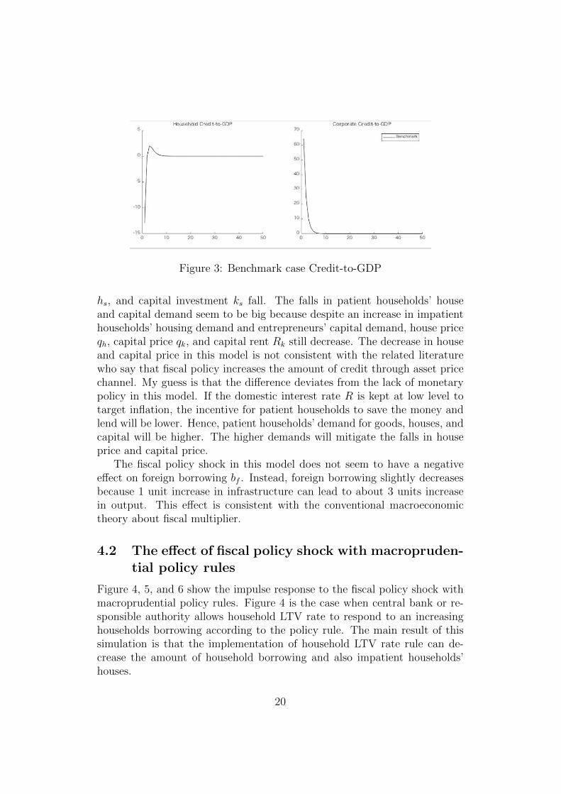
Figure 3: Benchmark case Credit-to-GDP

hs, and capital investment ks fall. The falls in patient households’ houseand capital demand seem to be big because despite an increase in impatienthouseholds’ housing demand and entrepreneurs’ capital demand, house priceqh, capital price qk, and capital rent Rk still decrease. The decrease in houseand capital price in this model is not consistent with the related literaturewho say that fiscal policy increases the amount of credit through asset pricechannel. My guess is that the difference deviates from the lack of monetarypolicy in this model. If the domestic interest rate R is kept at low level totarget inflation, the incentive for patient households to save the money andlend will be lower. Hence, patient households’ demand for goods, houses, andcapital will be higher. The higher demands will mitigate the falls in houseprice and capital price.

The fiscal policy shock in this model does not seem to have a negativeeffect on foreign borrowing bf . Instead, foreign borrowing slightly decreasesbecause 1 unit increase in infrastructure can lead to about 3 units increasein output. This effect is consistent with the conventional macroeconomictheory about fiscal multiplier.

4.2 The effect of fiscal policy shock with macropruden-tial policy rules

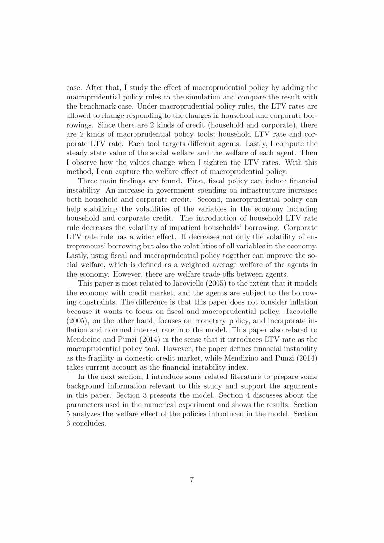
Figure 4, 5, and 6 show the impulse response to the fiscal policy shock withmacroprudential policy rules. Figure 4 is the case when central bank or re-sponsible authority allows household LTV rate to respond to an increasinghouseholds borrowing according to the policy rule. The main result of thissimulation is that the implementation of household LTV rate rule can de-crease the amount of household borrowing and also impatient households’houses.

20

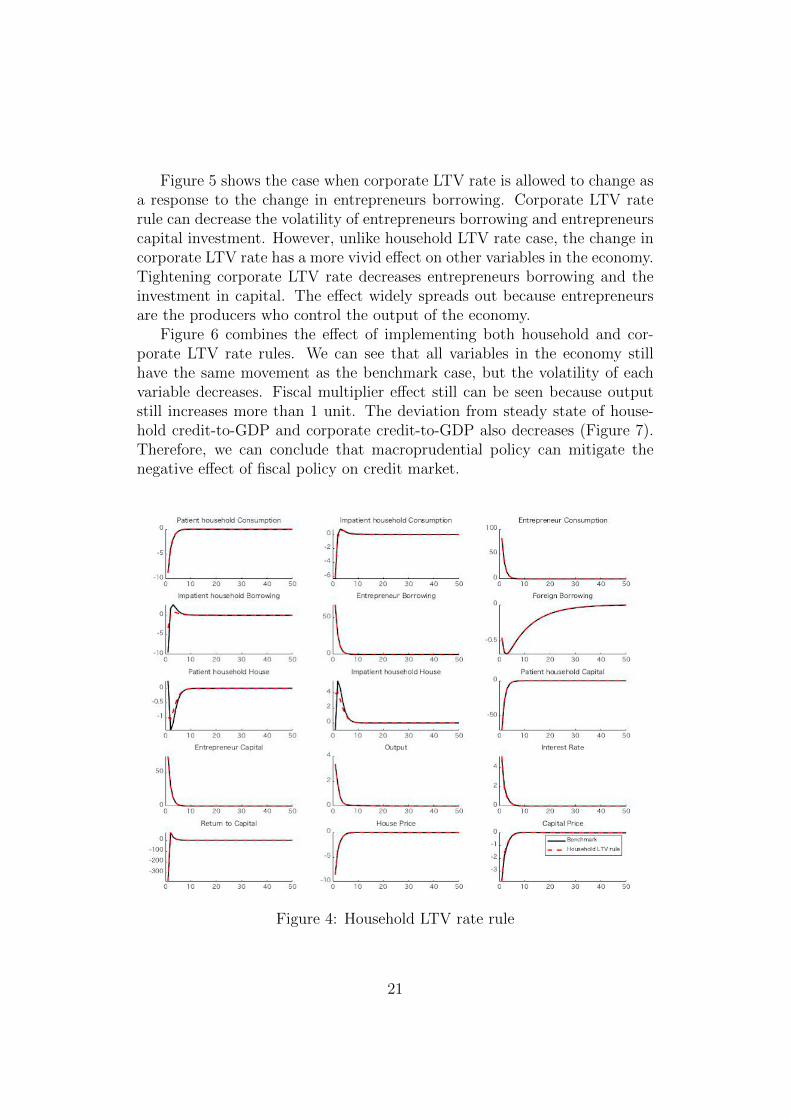
Figure 5 shows the case when corporate LTV rate is allowed to change asa response to the change in entrepreneurs borrowing. Corporate LTV raterule can decrease the volatility of entrepreneurs borrowing and entrepreneurscapital investment. However, unlike household LTV rate case, the change incorporate LTV rate has a more vivid effect on other variables in the economy.Tightening corporate LTV rate decreases entrepreneurs borrowing and theinvestment in capital. The effect widely spreads out because entrepreneursare the producers who control the output of the economy.

Figure 6 combines the effect of implementing both household and cor-porate LTV rate rules. We can see that all variables in the economy stillhave the same movement as the benchmark case, but the volatility of eachvariable decreases. Fiscal multiplier effect still can be seen because outputstill increases more than 1 unit. The deviation from steady state of house-hold credit-to-GDP and corporate credit-to-GDP also decreases (Figure 7).Therefore, we can conclude that macroprudential policy can mitigate thenegative effect of fiscal policy on credit market.

Figure 4: Household LTV rate rule

21

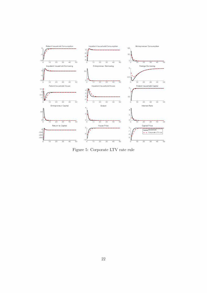
Figure 5: Corporate LTV rate rule

22

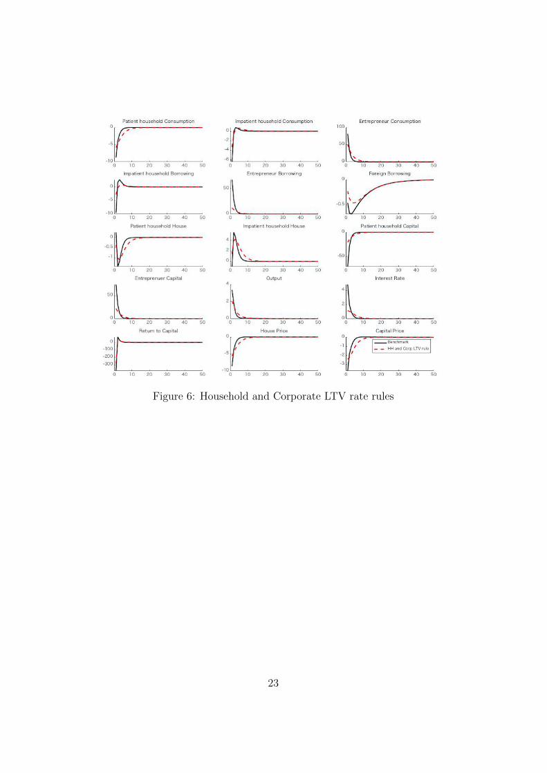
Figure 6: Household and Corporate LTV rate rules

23

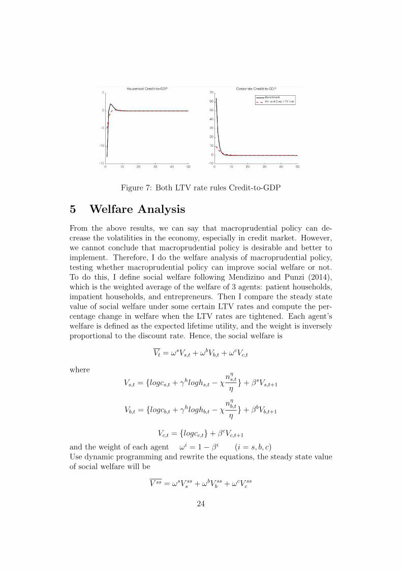
Figure 7: Both LTV rate rules Credit-to-GDP

5 Welfare Analysis

From the above results, we can say that macroprudential policy can de-crease the volatilities in the economy, especially in credit market. However,we cannot conclude that macroprudential policy is desirable and better toimplement. Therefore, I do the welfare analysis of macroprudential policy,testing whether macroprudential policy can improve social welfare or not.To do this, I define social welfare following Mendizino and Punzi (2014),which is the weighted average of the welfare of 3 agents: patient households,impatient households, and entrepreneurs. Then I compare the steady statevalue of social welfare under some certain LTV rates and compute the per-centage change in welfare when the LTV rates are tightened. Each agent’swelfare is defined as the expected lifetime utility, and the weight is inverselyproportional to the discount rate. Hence, the social welfare is

Vt = ωsVs,t + ωbVb,t + ωcVc,t

where

Vs,t = {logcs,t + γhloghs,t − χnηs,tη}+ βsVs,t+1

Vb,t = {logcb,t + γhloghb,t − χnηb,tη}+ βbVb,t+1

Vc,t = {logcc,t}+ βcVc,t+1

and the weight of each agent ωi = 1− βi (i = s, b, c)Use dynamic programming and rewrite the equations, the steady state valueof social welfare will be

V ss = ωsV sss + ωbV ss

b + ωcV ssc

24

where

V sss = {logcsss + γhloghsss − χ

nsssη

η}+ βsV ss

s

V ssb = {logcssb + γhloghssb − χ

nssbη

η}+ βbV ss

b

V ssc = {logcssc }+ βcV ss

c .

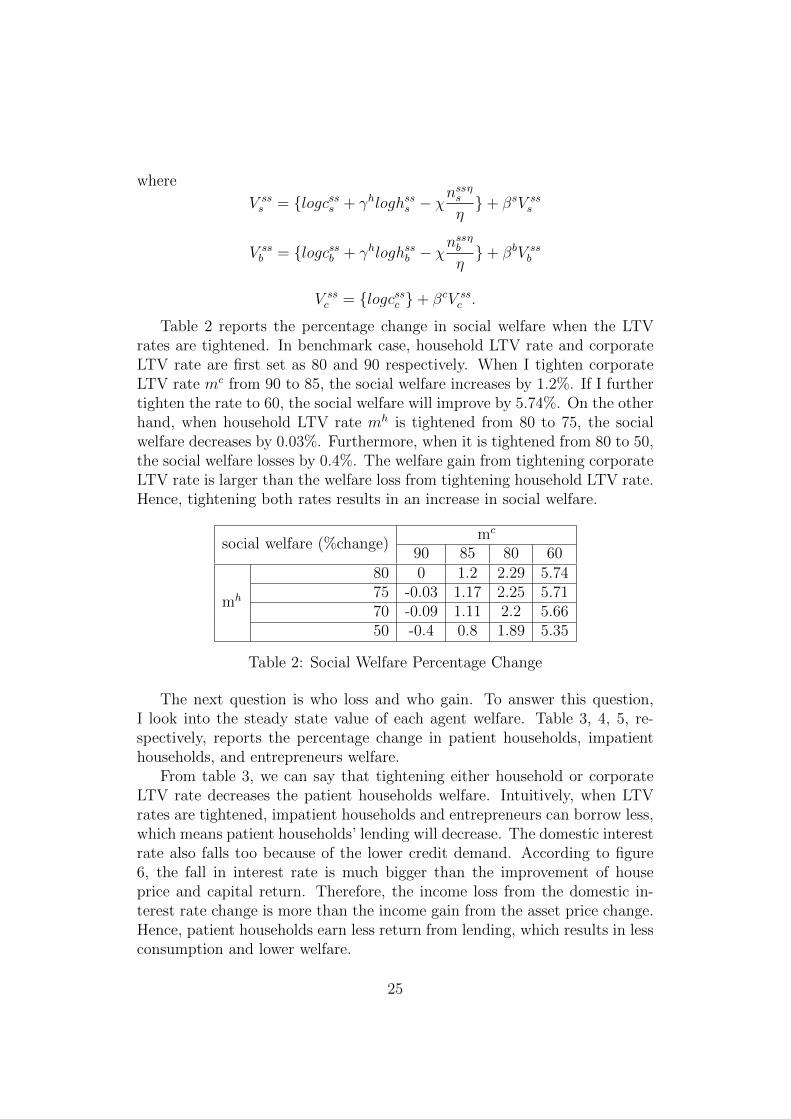
Table 2 reports the percentage change in social welfare when the LTVrates are tightened. In benchmark case, household LTV rate and corporateLTV rate are first set as 80 and 90 respectively. When I tighten corporateLTV rate mc from 90 to 85, the social welfare increases by 1.2%. If I furthertighten the rate to 60, the social welfare will improve by 5.74%. On the otherhand, when household LTV rate mh is tightened from 80 to 75, the socialwelfare decreases by 0.03%. Furthermore, when it is tightened from 80 to 50,the social welfare losses by 0.4%. The welfare gain from tightening corporateLTV rate is larger than the welfare loss from tightening household LTV rate.Hence, tightening both rates results in an increase in social welfare.

social welfare (%change)mc

90 85 80 60

mh

80 0 1.2 2.29 5.7475 -0.03 1.17 2.25 5.7170 -0.09 1.11 2.2 5.6650 -0.4 0.8 1.89 5.35

Table 2: Social Welfare Percentage Change

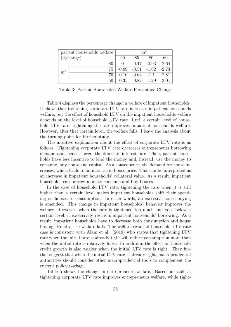
The next question is who loss and who gain. To answer this question,I look into the steady state value of each agent welfare. Table 3, 4, 5, re-spectively, reports the percentage change in patient households, impatienthouseholds, and entrepreneurs welfare.

From table 3, we can say that tightening either household or corporateLTV rate decreases the patient households welfare. Intuitively, when LTVrates are tightened, impatient households and entrepreneurs can borrow less,which means patient households’ lending will decrease. The domestic interestrate also falls too because of the lower credit demand. According to figure6, the fall in interest rate is much bigger than the improvement of houseprice and capital return. Therefore, the income loss from the domestic in-terest rate change is more than the income gain from the asset price change.Hence, patient households earn less return from lending, which results in lessconsumption and lower welfare.

25

patient households welfare(%change)

mc

90 85 80 60

mh

80 0 -0.47 -0.93 -2.6475 -0.09 -0.51 -1.02 -2.7370 -0.16 -0.64 -1.1 -2.8150 -0.35 -0.82 -1.29 -3.01

Table 3: Patient Households Welfare Percentage Change

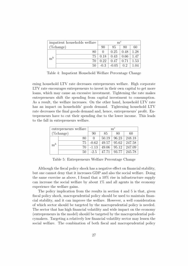
Table 4 displays the percentage change in welfare of impatient households.It shows that tightening corporate LTV rate increases impatient householdswelfare, but the effect of household LTV on the impatient households welfaredepends on the level of household LTV rate. Until a certain level of house-hold LTV rate, tightening the rate improves impatient households welfare.However, after that certain level, the welfare falls. I leave the analysis aboutthe turning point for further study.

The intuitive explanation about the effect of corporate LTV rate is asfollows. Tightening corporate LTV rate decreases entrepreneurs borrowingdemand and, hence, lowers the domestic interest rate. Then, patient house-holds have less incentive to lend the money and, instead, use the money toconsume, buy house and capital. As a consequence, the demand for house in-creases, which leads to an increase in house price. This can be interpreted asan increase in impatient households’ collateral value. As a result, impatienthouseholds can borrow more to consume and buy houses.

In the case of household LTV rate, tightening the rate when it is stillhigher than a certain level makes impatient households shift their spend-ing on houses to consumption. In other words, an excessive house buyingis amended. This change in impatient households’ behavior improves thewelfare. However, when the rate is tightened too much and goes below acertain level, it excessively restricts impatient households’ borrowing. As aresult, impatient households have to decrease both consumption and housebuying. Finally, the welfare falls. The welfare result of household LTV ratecase is consistent with Alam et al. (2019) who states that tightening LTVrate when the initial rate is already tight will reduce consumption more thanwhen the initial rate is relatively loose. In addition, the effect on householdcredit growth is also weaker when the initial LTV rate is tight. They fur-ther suggest that when the initial LTV rate is already tight, macroprudentialauthorities should consider other macroprudential tools to complement thecurrent policy package.

Table 5 shows the change in entrepreneurs welfare. Based on table 5,tightening corporate LTV rate improves entrepreneurs welfare, while tight-

26

impatient households welfare(%change)

mc

90 85 80 60

mh

80 0 0.25 0.48 1.2875 0.18 0.43 0.66 1.4770 0.22 0.47 0.71 1.5350 -0.3 -0.05 0.2 1.04

Table 4: Impatient Household Welfare Percentage Change

ening household LTV rate decreases entrepreneurs welfare. High corporateLTV rate encourages entrepreneurs to invest in their own capital to get moreloans, which may cause an excessive investment. Tightening the rate makesentrepreneurs shift the spending from capital investment to consumption.As a result, the welfare increases. On the other hand, household LTV ratehas an impact on households’ goods demand. Tightening household LTVrate decreases the final goods demand and, hence, entrepreneurs’ profit. En-trepreneurs have to cut their spending due to the lower income. This leadsto the fall in entrepreneurs welfare.

entrepreneurs welfare(%change)

mc

90 85 80 60

mh

80 0 50.19 96.23 248.1875 -0.62 49.57 95.62 247.5870 -1.13 49.06 95.12 247.0950 -2.5 47.71 93.77 245.78

Table 5: Entrepreneurs Welfare Percentage Change

Although the fiscal policy shock has a negative effect on financial stability,but one cannot deny that it increases GDP and also the social welfare. Doingthe same exercise as above, I found that a 10% rise in infrastructure supplycan increase the social welfare by about 1% and all agents in the economyexperience the welfare gains.

The policy implication from the results in section 4 and 5 is that, givenfiscal policy shock, macroprudential policy should be used to maintain finan-cial stability, and it can improve the welfare. However, a well considerationof which sector should be targeted by the macroprudential policy is needed.The sector that has high financial volatility and wide impact on the economy(entrepreneurs in the model) should be targeted by the macroprudential poli-cymakers. Targeting a relatively low financial volatility sector may lessen thesocial welfare. The combination of both fiscal and macroprudential policy

27

makes it possible to maintain financial stability without restricting economicgrowth. In addition, it also improves the social welfare.

6 Conclusion

Along with economic growth, emerging countries are facing a rapid creditgrowth. Many international institutions and central banks start to be awareof the financial instability diverting from the increasing credit. It is timefor emerging countries to give more importance to financial stability besideseconomic growth and reconsider the policy packages.

This paper argues that fiscal policy, which is a famous economic stimuluspolicy, can induce financial instability. Concretely, the paper shows that anincrease in government spending on infrastructure, or the fiscal policy shockin the model, can lead to an increase in households and entrepreneurs bor-rowing from the steady state. The infrastructure contributes to an increasein output of the economy, and also the households’ and entrepreneurs’ in-comes. Households and entrepreneurs, then, buy more houses and capital,which are the assets that can be used as collateral, to get more loans. As aresult, households and entrepreneurs borrowings rise.

Even though the government spending on infrastructure has a side effect,the government cannot refrain from using this fiscal tool because infrastruc-ture is a main source of economic growth, and the infrastructure demand iscontinuously high in emerging countries. To solve this problem, I proposethe use of macroprudential policy. The macroprudential policy tools used inthis paper are rules on household LTV rate and corporate LTV rate. Whenthe LTV rates are allowed to respond to the change in households and en-trepreneurs borrowings, the rise in borrowings after the fiscal policy shockdecreases. In addition, tightening corporate LTV rate has a wider effect thantightening household LTV rate to the extent that it can reduce the volatilityof all variables in the economy. Even though macroprudential policy lessensthe effect of fiscal policy on output, we can still see a more-than-one fiscalmultiplier effect. The use of macroprudential policy under a given fiscal pol-icy improves the social welfare because it gives the incentives for householdsand entrepreneurs to shift their spending from houses and capital buyingto consumption. Tightening LTV rates prevent the excess collateral assets’buying behavior of households and entrepreneurs.

Based on the results, I suggest that macroprudential policy should be usedtogether with fiscal policy. The combination of fiscal and macroprudentialpolicy helps emerging countries to maintain financial stability and achieveeconomic growth at the same time, and it also improves the social welfare.

28

7 Appendix

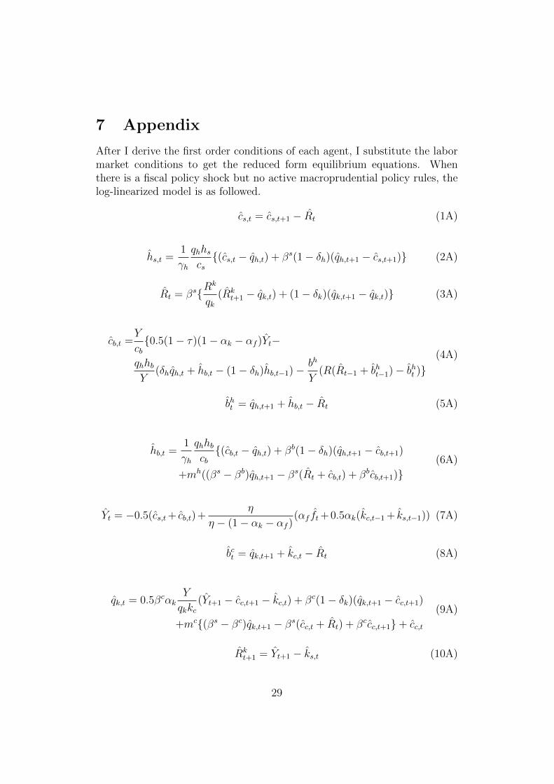
After I derive the first order conditions of each agent, I substitute the labormarket conditions to get the reduced form equilibrium equations. Whenthere is a fiscal policy shock but no active macroprudential policy rules, thelog-linearized model is as followed.

cs,t = cs,t+1 − Rt (1A)

hs,t =1

γh

qhhscs{(cs,t − qh,t) + βs(1− δh)(qh,t+1 − cs,t+1)} (2A)

Rt = βs{Rk

qk(Rk

t+1 − qk,t) + (1− δk)(qk,t+1 − qk,t)} (3A)

cb,t =Y

cb{0.5(1− τ)(1− αk − αf )Yt−

qhhbY

(δhqh,t + hb,t − (1− δh)hb,t−1)−bh

Y(R(Rt−1 + bht−1)− bht )}

(4A)

bht = qh,t+1 + hb,t − Rt (5A)

hb,t =1

γh

qhhbcb{(cb,t − qh,t) + βb(1− δh)(qh,t+1 − cb,t+1)

+mh((βs − βb)qh,t+1 − βs(Rt + cb,t) + βbcb,t+1)}(6A)

Yt = −0.5(cs,t+ cb,t) +η

η − (1− αk − αf )(αf ft+ 0.5αk(kc,t−1 + ks,t−1)) (7A)

bct = qk,t+1 + kc,t − Rt (8A)

qk,t = 0.5βcαkY

qkkc(Yt+1 − cc,t+1 − kc,t) + βc(1− δk)(qk,t+1 − cc,t+1)

+mc{(βs − βc)qk,t+1 − βs(cc,t + Rt) + βccc,t+1}+ cc,t

(9A)

Rkt+1 = Yt+1 − ks,t (10A)

29

cc,t =Y

cc{(αk + αf )Yt −

qkkcY

(δkqk,t + kc,t − (1− δk)kc,t+1)

−RkksY

(Rkt + ks,t−1) +

bc

Y(bct −R(Rc

t−1 + bct−1))}(11A)

b∗t =Y

eb∗{ fYft − τ(1− αk − αf )Yt}+R∗b∗t−1 (12A)

Yt =csYcs,t +

cbYcb,t +

f

Yft +

eb∗

Y(R∗b∗t−1 − b∗t ) (13A)

hs,t = −hbhshb,t (14A)

ks,t = −kckskc,t (15A)

ft = ρf ft−1 + εf (16A)

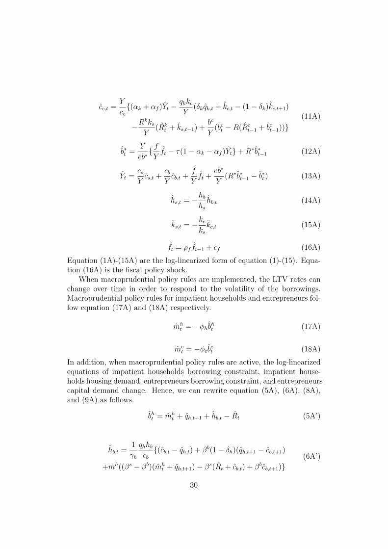
Equation (1A)-(15A) are the log-linearized form of equation (1)-(15). Equa-tion (16A) is the fiscal policy shock.

When macroprudential policy rules are implemented, the LTV rates canchange over time in order to respond to the volatility of the borrowings.Macroprudential policy rules for impatient households and entrepreneurs fol-low equation (17A) and (18A) respectively.

mht = −φhbht (17A)

mct = −φcbct (18A)

In addition, when macroprudential policy rules are active, the log-linearizedequations of impatient households borrowing constraint, impatient house-holds housing demand, entrepreneurs borrowing constraint, and entrepreneurscapital demand change. Hence, we can rewrite equation (5A), (6A), (8A),and (9A) as follows.

bht = mht + qh,t+1 + hb,t − Rt (5A’)

hb,t =1

γh

qhhbcb{(cb,t − qh,t) + βb(1− δh)(qh,t+1 − cb,t+1)

+mh((βs − βb)(mht + qh,t+1)− βs(Rt + cb,t) + βbcb,t+1)}

(6A’)

30

bct = mct + qk,t+1 + kc,t − Rt (8A’)

qk,t = 0.5βcαkY

qkkc(Yt+1 − cc,t+1 − kc,t) + βc(1− δk)(qk,t+1 − cc,t+1)

+mc{(βs − βc)(mct + qk,t+1)− βs(cc,t + Rt) + βccc,t+1}+ cc,t

(9A’)

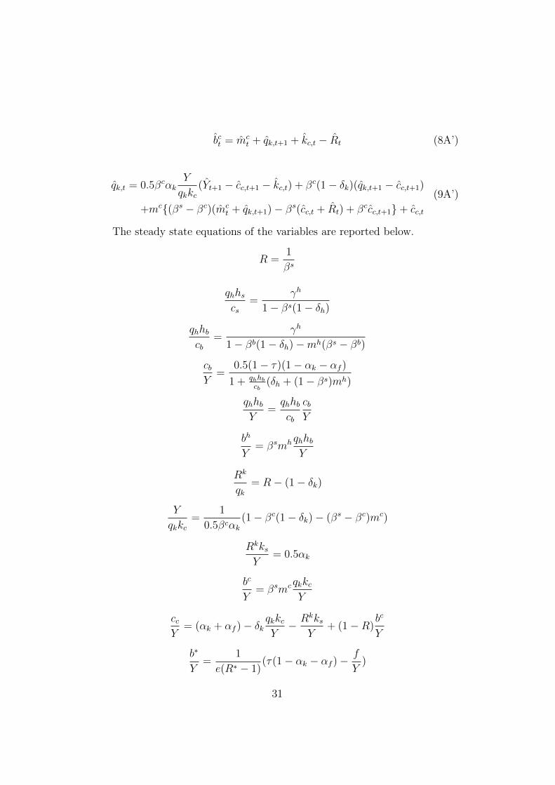
The steady state equations of the variables are reported below.

R =1

βs

qhhscs

=γh

1− βs(1− δh)

qhhbcb

=γh

1− βb(1− δh)−mh(βs − βb)

cbY

=0.5(1− τ)(1− αk − αf )

1 + qhhbcb

(δh + (1− βs)mh)

qhhbY

=qhhbcb

cbY

bh

Y= βsmh qhhb

Y

Rk

qk= R− (1− δk)

Y

qkkc=

1

0.5βcαk(1− βc(1− δk)− (βs − βc)mc)

RkksY

= 0.5αk

bc

Y= βsmc qkkc

Y

ccY

= (αk + αf )− δkqkkcY− Rkks

Y+ (1−R)

bc

Y

b∗

Y=

1

e(R∗ − 1)(τ(1− αk − αf )−

f

Y)

31

csY

= 1− cbY− ccY− f

Y− e(R∗ − 1)

b∗

Y

hbhs

=qhhbY

/(qhhscs

csY

)

kcks

= (qkkcY

Rk

qk)/RkksY

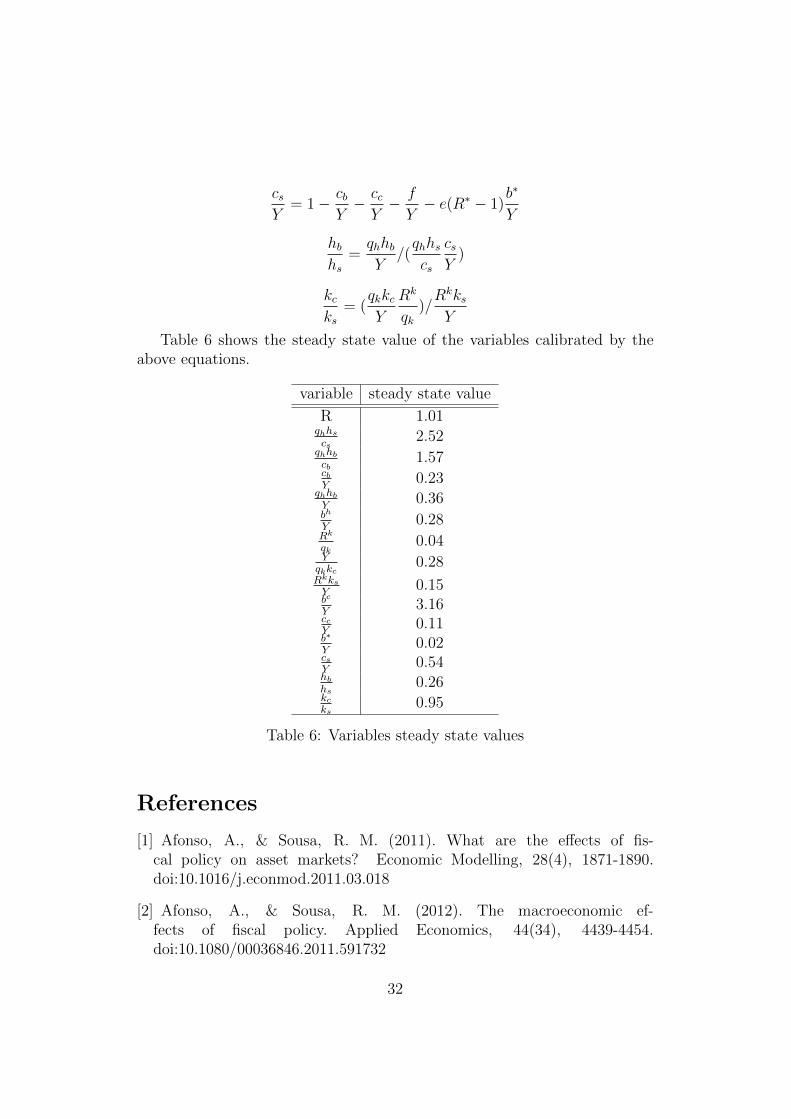
Table 6 shows the steady state value of the variables calibrated by theabove equations.

variable steady state value

R 1.01qhhscs

2.52qhhbcb

1.57cbY

0.23qhhbY

0.36bh

Y0.28

Rk

qk0.04

Yqkkc

0.28RkksY

0.15bc

Y3.16

ccY

0.11b∗

Y0.02

csY

0.54hbhs

0.26kcks

0.95

Table 6: Variables steady state values

References

[1] Afonso, A., & Sousa, R. M. (2011). What are the effects of fis-cal policy on asset markets? Economic Modelling, 28(4), 1871-1890.doi:10.1016/j.econmod.2011.03.018

[2] Afonso, A., & Sousa, R. M. (2012). The macroeconomic ef-fects of fiscal policy. Applied Economics, 44(34), 4439-4454.doi:10.1080/00036846.2011.591732

32

[3] Agnello, L., & Schuknecht, L. (2011). Booms andbusts in housing markets: Determinants and implicationsdoi:https://doi.org/10.1016/j.jhe.2011.04.001

[4] Alam, Z., Alter, A., Eiseman, J., G Gelos, R., Kang, H., Narita,M., . . . Wang, N. (2019). Digging deeper–evidence on the effects ofmacroprudential policies from a new database. ().International MonetaryFund. doi:DOI: Retrieved from https://ideas.repec.org/p/imf/imfwpa/19-66.html

[5] Alpanda, S., & Zubairy, S. (2016). Housing and tax policy. Journal ofMoney Credit and Banking, 48(2-3), 485-512. doi:10.1111/jmcb.12307

[6] Alpanda, S., & Zubairy, S. (2017). Addressing household indebtedness:Monetary, fiscal or macroprudential policy? European Economic Review,92, 47-73. doi:10.1016/j.euroecorev.2016.11.004

[7] AMRO. (2018). ASEAN+3 regional economic outlook 2018. Retrievedfrom https://amro-asia.org/wp-content/uploads/2018/05/AMRO-AREO-Report-2018 Full-Report.pdf

[8] Aoki, K., Benigno, G. and Kiyotaki, N. (2018). Monetary and financialpolicies in emerging markets. Mimeo, Princeton University

[9] Bank of Thailand. (2017). Financial Stability Report 2017. Retrievedfrom https://www.bot.or.th/English/FinancialInstitutions/Publications/FSR Doc/FSR2017e.pdf

[10] Calderon, C., Moral-Benito, E., & Serven, L. (2015). Is infrastructurecapital productive? A dynamic heterogeneous approach. Journal of Ap-plied Econometrics, 30(2), 177-198. doi:10.1002/jae.2373

[11] Carvalho, F. A., & Castro, M. R. (2017). Macroprudential pol-icy transmission and interaction with fiscal and monetary policyin an emerging economy: A DSGE model for brazil. Macroeco-nomics and Finance in Emerging Market Economies, 10(3), 215-259.doi:10.1080/17520843.2016.1270982

[12] Cerutti, E., Claessens, S., & Laeven, L. (2017). The useand effectiveness of macroprudential policies: New evidencedoi:https://doi.org/10.1016/j.jfs.2015.10.004

[13] Chen, S., & Kang, J. (2018). Credit booms-is china different? IMFWorking Papers, 18, 1. doi:10.5089/9781484336762.001

33

[14] Claessens, S. (2014). An overview of macroprudential policytools. ().International Monetary Fund. doi:DOI: Retrieved fromhttps://ideas.repec.org/p/imf/imfwpa/14-214.html

[15] Croce, M. M., Kung, H., Nguyen, T. T., & Schmid, L. (2012). Fiscalpolicies and asset prices. Review of Financial Studies, 25(9), 2635-2672.doi:10.1093/rfs/hhs060

[16] Dumicic, M. (2019). Linkages between fiscal policy and financial(in)stability. Journal of Central Banking Theory and Practice, 8(1), 97-109. doi:10.2478/jcbtp-2019-0005

[17] Freixas, X., Laeven, L., & Peydro, J. (2015). Systemic risk,crises, and macroprudential regulation Mit Press. Retrieved fromhttp://www.jstor.org/stable/j.ctt17kk82g

[18] Galati, G. (2018). What do we know about the effects of macroprudentialpolicy? Economica (London), 85(340), 735; 735-770; 770.

[19] Garbers, C., & Liu, G. (2018). Macroprudential policy and foreigninterest rate shocks: A comparison of loan-to-value and capital re-quirements. International Review of Economics & Finance, 58, 683-698.doi:10.1016/j.iref.2018.07.008

[20] Garcia-Escribano, Mercedes,Han, Fei,. (2015). Credit expansion inemerging markets propeller of growth?

[21] Haldane, A. G., & May, R. M. (2011). Systemic risk in banking ecosys-tems. Nature, 469(7330), 351-355. doi:10.1038/nature09659

[22] Hallett, A. H., Libich, J., & Stehlik, P. (2011). Macroprudentialpolicies and financial stability*. Economic Record, 87(277), 318-334.doi:10.1111/j.1475-4932.2010.00692.x

[23] Haruhiko, Kuroda. (2019). For Sustainable Development of EmergingEconomies. Bank of Japan

[24] Hodula, M. (2018). Fiscal-monetary-financial stability interactions in adata-rich environment. Review of Economic Perspectives, 18(3), 195; 195-224; 224.

[25] Iacoviello, M. (2005). House prices, borrowing constraints, and mone-tary policy in the business cycle. American Economic Review, 95(3), 739-764.doi:DOI: ,

34

[26] JORDA, O., SCHULARICK, M., & TAYLOR, A. M. (2013). Whencredit bites back. Journal of Money, Credit and Banking, 45, 3-28.doi:10.1111/jmcb.12069

[27] Kara, H. (2016). Turkey’s experience with macroprudential policy. (pp.123-139) Bank for International Settlements. doi:DOI: Retrieved fromhttps://ideas.repec.org/h/bis/bisbpc/86-17.html

[28] Kenneth, N. K., & Shim, I. (2013). Can non-interest rate poli-cies stabilise housing markets? evidence from a panel of 57economies. ().Bank for International Settlements. doi:DOI: Retrieved fromhttps://ideas.repec.org/p/bis/biswps/433.html

[29] IMF. (2013). Key aspects of macroprudential policy. Policy Papers,2013(82)

[30] Kiyotaki, N., & Moore, J. (1997). Credit cycles. Journal of PoliticalEconomy, 105(2), 211-248. doi:10.1086/262072

[31] Lambertini, L., Mendicino, C., & Punzi, M. T. (2017). Expectations-driven cycles in the housing market. Economic Modelling, 60, 297-312.doi:10.1016/j.econmod.2016.10.004

[32] Mendicino, C., & Punzi, M. T. (2014). House prices, capital inflowsand macroprudential policy. Journal of Banking Finance, 49, 337-355.doi:10.1016/j.jbankfin.2014.06.007

[33] Morgan, P. J., Regis, P. J., & Salike, N. (2019). LTV policy as a macro-prudential tool and its effects on residential mortgage loans. Journal ofFinancial Intermediation, 37, 89-103. doi:10.1016/j.jfi.2018.10.001

[34] Nier, E., & Kang, H. (2016). Monetary and macroprudential poli-cies exploring interactions. In B. f. I. Settlements (Ed.), Macropruden-tial policy (pp. 27-38) Bank for International Settlements. Retrieved fromhttps://EconPapers.repec.org/RePEc:bis:bisbpc:86-05

[35] Oscar Jorda, Schularick, M., & Alan, M. T. (2011). Financial crises,credit booms, and external imbalances: 140 years of lessons. IMF Eco-nomic Review, 59(2), 340-378. doi:DOI: ,

[36] Punzi, M. T., & Rabitsch, K. (2018). Effectiveness of macroprudentialpolicies under borrower heterogeneity. Journal of International Money andFinance, 85, 251-261. doi:10.1016/j.jimonfin.2017.11.008

35

[37] Townsend, R., & Ueda, K. (2010). Welfare gains from finan-cial liberalization*. International Economic Review, 51(3), 553-597.doi:10.1111/j.1468-2354.2010.00593.x

[38] UBS. (2018). Longer Term Investment: Emerg-ing market infrastructure–update. Retrieved fromhttps://www.ubs.com/content/dam/WealthManagementAmericas/documents/em-infrastructure.pdf

[39] UNECE. (2016). No.3 Sustainable developmentbrief : Infrastructure and Growth. Retrieved fromhttps://www.unece.org/fileadmin/DAM/Brief No 3

Infrastructure and Growth.pdf

36