The Interaction of High-Power Lasers with Plasmasastro · comprehensive and useful presentation of laser–plasma interaction. The book describes the laser absorption and propagation

The Interaction of High-Power Lasers with Plasmas

Series in Plasma Physics

Series Editors:

Steve Cowley, Imperial College, UKPeter Stott, CEA Cadarache, FranceHans Wilhelmsson, Chalmers University of Technology, Sweden

Other books in the series

Introduction to Dusty Plasma Physics

P K Shukla and A A Mamum

The Theory of Photon Acceleration

J T Mendonca

Laser Aided Diagnostics of Plasmas and Gases

K Muraoka and M Maeda

Reaction-Diffusion Problems in the Physics of Hot Plasmas

H Wilhelmsson and E Lazzaro

The Plasma Boundary of Magnetic Fusion Devices

P C Stangeby

Non-Linear Instabilities in Plasmas and Hydrodynamics

S S Moiseev, V N Oraevsky and V G Pungin

Collective Modes in Inhomogeneous Plasmas

J Weiland

Transport and Structural Formation in Plasmas

K Itoh, S-I Itoh and A Fukuyama

Tokamak Plasmas: A Complex Physical System

B B Kadomstev

Forthcoming titles in the series

Microscopic Dynamics of Plasmas and Chaos

Y Elskens and D Escande

Nonlinear Plasma Physics

P K Shukla

Series in Plasma Physics

The Interaction of High-Power Lasers

with Plasmas

Shalom Eliezer

Plasma Physics Department, Soreq N.R.C.,Yavne, IsraelandInstitute of Nuclear Fusion,Madrid Polytechnic University, Madrid, Spain

Institute of Physics PublishingBristol and Philadelphia

# IOP Publishing Ltd 2002

All rights reserved. No part of this publication may be reproduced, stored ina retrieval system or transmitted in any form or by any means, electronic,mechanical, photocopying, recording or otherwise, without the priorpermission of the publisher. Multiple copying is permitted in accordancewith the terms of licences issued by the Copyright Licensing Agency underthe terms of its agreement with Universities UK (UUK).

British Library Cataloguing-in-Publication Data

A catalogue record of this book is available from the British Library.

ISBN 0 7503 0747 1

Library of Congress Cataloging-in-Publication Data are available

Commissioning Editor: John NavasProduction Editor: Simon LaurensonProduction Control: Sarah PlentyCover Design: Victoria Le BillonMarketing: Nicola Newey and Verity Cooke

Published by Institute of Physics Publishing, wholly owned byThe Institute of Physics, London

Institute of Physics Publishing, Dirac House, Temple Back,Bristol BS1 6BE, UK

US Office: Institute of Physics Publishing, The Public Ledger Building,Suite 929, 150 South Independence Mall West, Philadelphia,PA 19106, USA

Typeset by Academic þ Technical, BristolPrinted in the UK by J W Arrowsmith Ltd, Bristol

Preface

This book covers the physics of high-power laser interaction with plasmas,a subject related to both fundamental physics and the applied sciences.The book covers high-power laser irradiation, from low-laser intensityIL � 109 W/cm2 up to extremely high intensities IL � 1020 W/cm2, and forlaser pulse duration between �L � 10 nanoseconds to as short as �L � 10femtoseconds. The plasma medium varies from low densities (dilute gases)to very high densities (highly-compressed solid state). The relevant tempera-tures can change over many orders of magnitude, and electric and magneticfields can reach enormously high values.

The interaction of high-power lasers with matter should be of interestto people from different branches of science who may be unfamiliar withplasma science. Therefore, the relevant basic plasma physics is developedand explained in detail. Three basic approaches to plasma physics areconsidered, namely the two fluids model, the Boltzmann–Vlasov equationsand the particle simulation method.

This book is not a summary of research results, but rather it is apedagogical presentation where the basic physics issues are addressed andsimple models are used wherever appropriate. The material covered couldserve as a good foundation on which the undergraduate as well as thegraduate student can build an understanding of the past and present researchin this field. For the experienced researcher, I hope that this book is acomprehensive and useful presentation of laser–plasma interaction.

The book describes the laser absorption and propagation by a plasmamedium, the electron transport phenomenon and the analysis of the relevantplasma waves. The physics of the electric and magnetic fields in a laser-induced plasma medium is comprehensively described. The subjects oflaser-induced shock waves, rarefaction waves, heat waves and the relatedhydrodynamic instabilities (Rayleigh–Taylor, Richtmyer–Meshkov andKelvin–Helmholtz) are developed and discussed. The very important subjectof applications was purposely omitted as it merits a volume of its own.

v

A prerequisite in plasma physics is to know and master both systems ofunits: the m.k.s., known as the SI (International System) units, and the c.g.s.–Gaussian units. Furthermore, one of the most useful physical quantities is thelaser intensity (energy flux) IL, which is usually given in mixed units (Watts/cm2). Although most of the time the c.g.s.–Gaussian units are chosen, bothsystems of units are used, in addition to the practical units such as electron-volt (eV) for energy or temperature.

I would like to thank my colleagues from the plasma physics departmentat Soreq in Yavne, Israel, and from the Institute of Nuclear Fusion at thePolytechnic University in Madrid, Spain, for the fruitful discussions whichwere very inspiring, stimulating and useful. I am grateful to D. Fisher forhis critical reading of the manuscript and to Y. Paiss for the valuablediscussions regarding the first chapter of this book. I greatly acknowledgethe help from A. Borowitz, E. Dekel and M. Fraenkel for their help withthe technical problems in preparing the manuscript. My thanks are alsoextended to R. Naem for the preparation of the figures. Last, but notleast, my deep appreciation to my wife Yaffa for her encouragement towrite the book and to bear with me to its successful completion.

vi Preface

Contents

1 High Power Lasers, from Nanoseconds to Femtoseconds 1

1.1 Basics 21.2 A Stroll through a Glass Laser System 7

1.2.1 The oscillator 81.2.2 The amplifiers 91.2.3 Spatial filters 101.2.4 Isolators 101.2.5 Diagnostics 10

1.3 Highlights of the Femtosecond Laser 11

2 Introduction to Plasma Physics for Electrons and Ions 14

2.1 Ionization 142.2 Cross Section, Mean Free Path and Collision Frequency 172.3 Transport Coefficients 22

2.3.1 Electrical conductivity 222.3.2 Thermal conductivity 232.3.3 Diffusion 242.3.4 Viscosity 26

2.4 Radiation Conductivity 272.4.1 Bound–bound (bb) transitions 272.4.2 Bound–free (bf ) transitions 282.4.3 Free–free (ff ) transitions 282.4.4 Energy transport 28

2.5 Debye Length 332.6 Plasma Oscillations and Electron Plasma Waves 362.7 The Dielectric Function 402.8 The Laser-Induced Plasma Medium 42

3 The Three Approaches to Plasma Physics 47

3.1 Fluid Equations 473.1.1 Mass conservation 47

vii

3.1.2 Momentum conservation 483.1.3 Energy conservation 49

3.2 Eulerian and Lagrangian Coordinates 513.3 ‘Femtosecond’ Laser Pulses 543.4 Boltzmann–Vlasov Equations 55

3.4.1 Liouville’s theorem 553.4.2 Vlasov equation 563.4.3 Boltzmann equation 573.4.4 The moment equations 58

3.5 Particle Simulations 61

4 The Ponderomotive Force 65

4.1 The Landau–Lifshitz Ponderomotive Force 654.2 The Single-Particle Approach to Ponderomotive Force in

Plasma 684.3 The Effect of Ponderomotive Force on Wave Dispersion 69

4.3.1 The electron wave dispersion 694.3.2 The ion wave dispersion 71

5 Laser Absorption and Propagation in Plasma 74

5.1 Collisional Absorption (Inverse Bremsstrahlung) 745.2 The Electromagnetic Wave Equation in a Plasma Medium 795.3 Slowly Varying Density—the WKB Approximation 815.4 Linear Varying Density—the Airy Functions 845.5 Obliquely Incident Linearly Polarized Laser 88

5.5.1 s-polarization 905.6 p-Polarization: the Resonance Absorption 915.7 Femtosecond Laser Pulses 96

6 Waves in Laser-Produced Plasma 105

6.1 Foreword to Parametric Instabilities 1056.2 The Forced Harmonic Oscillator 1106.3 Landau Damping 1126.4 Parametric Decay Instability 1156.5 Stimulated Brillouin Scattering 1206.6 A Soliton Wave 124

6.6.1 A historical note 1246.6.2 What is a soliton? 1266.6.3 What is a solitary wave? 1266.6.4 The wave equation 1266.6.5 Ion plasma wave and the KdV equation 127

7 Laser-Induced Electric Fields in Plasma 134

7.1 High- and Low-Frequency Electric Fields 134

viii Contents

7.2 Expansion of Plasma into the Vacuum 1357.3 Double Layers 1387.4 Charged Particle Acceleration 140

7.4.1 A static model 1407.4.2 A dynamic model 141

8 Laser-Induced Magnetic Fields in Plasma 144

8.1 The rn�rT Toroidal Magnetic Field 1458.2 Magneto-Hydrodynamics and the Evolution of the

Magnetic Field 1468.2.1 The generalized Ohm’s law 1478.2.2 The magnetic Reynolds number 1518.2.3 Magnetic Reynolds numbers Rm � 1 1518.2.4 Magnetic Reynolds numbers Rm � 1 152

8.3 Faraday and Inverse Faraday Effects 1538.3.1 The Faraday effect 1538.3.2 The inverse Faraday effect 1578.3.3 Angular momentum considerations 159

8.4 Waves in the Presence of the Steady-State Magnetic Field 1628.4.1 Ordinary and Extraordinary Waves 1628.4.2 Electromagnetic waves propagating parallel to B0 1658.4.3 Alfven waves 168

8.5 Resonance Absorption in a Magnetized Plasma 169

9 Thermal Conduction and Heat Waves 175

9.1 The Scenario 1759.2 The Rocket Model 1809.3 Relaxation Rates 1839.4 The Fokker–Planck Equation 1899.5 The Spitzer–Harm Conductivity 1959.6 Hot Electrons 1989.7 Heat Waves 205

10 Shock Waves and Rarefaction Waves 213

10.1 A Perspective 21310.2 Sound Waves 21610.3 Rarefaction Waves 21910.4 Shock Waves 22110.5 Shock Waves in the Presence of Magnetic Fields 23310.6 The Study of High-Pressure Physics 23710.7 Studies of Equations of State 24110.8 Studies of Dynamic Strength of Materials 249

Contents ix

11 Hydrodynamic Instabilities 254

11.1 Background 25411.2 Rayleigh–Taylor Instability, Linear Analysis 26011.3 Ablation-Surface Instability 26411.4 The Magnetic Field Effect 26611.5 Bubbles from Rayleigh–Taylor Instability 26911.6 Richtmyer–Meshkov Instability 272

11.6.1 The differential equation for the pressure in regions 1and 2 275

11.6.2 The boundary conditions on the interface 27611.6.3 The boundary conditions at the shock-wave surfaces 276

11.7 Kelvin–Helmholtz Instability 279

Appendix A: Maxwell Equations 284

Appendix B: Prefixes 290

Appendix C: Vectors and Matrices 291

Appendix D: A Note on the Maxwell Distribution 297

Bibliography 300

Index 309

x Contents

Chapter 1

High Power Lasers, from Nanoseconds

to Femtoseconds

This chapter is an introduction to high power lasers and it is intended topresent the principles and the parameters of such systems. Lasers (acronymof light amplification by stimulated emission of radiation) are devices thatgenerate or amplify electromagnetic radiation, ranging from the longinfrared region up through the visible region and extending to the ultravioletand recently even to the x-ray region (Ross 1968, Sargent et al. 1974, Svelto1976, Thyagarajan and Ghatak 1981, Siegman 1986, Elton 1990, Dielsand Rudolph 1996 and Robieux 2000). The 1964 Nobel Prize for physicswas shared between Charles Townes, Nikolai Basov and AlexanderProkhorov for their fundamental work in the 1950s that led to the construc-tion of the laser.

Maiman demonstrated the first laser in 1960; the lasing medium wasa ruby crystal, pumped by xenon flash discharge, and the pulse durationwas between 1ms and 1 ms (Maiman 1960). In 1961 Hellwarth invented theconcept of Q switching and put it into practice with a ruby laser by using aKerr cell shutter. Hellwarth reported (Hellwarth 1961) a pulse duration ofabout 10 nanoseconds (1 nanosecond¼ 1 ns¼ 10�9 s).

The first active mode locking was achieved in 1964 for a helium–neonlaser yielding a laser with pulse duration above 1 ns. The mode lockingwas achieved by modulating the index of refraction acoustically at theperiod that the light travels (a round trip) in the cavity (Hargrove et al.1964). Using a saturable absorber, the idea of passive mode locking wassuggested (Mocker and Collins 1965), and in 1966 a neodymium glass laserpulse shorter than a nanosecond was first obtained (DeMaria et al. 1966).Today pulses of the order of 10 picosecond (1 picosecond¼ 1 ps¼ 10�12 s)duration are common in many laboratories around the world. In the pastdecade 10 femtosecond (1 femtosecond¼ 1 fs¼ 10�15 s) pulses were achievedfrom a Ti–sapphire laser (Zhou et al. 1994, Glezer 1997). The chirped pulse

amplification technique (used in microwave devices for many years) wasfirst suggested for the lasers in 1985 (Strickland and Mourou 1985) in

1

order to amplify short laser pulses. In this scheme the femtosecond laser pulseis first stretched in time (chirped in frequency), then amplified and finallyrecompressed (Perry and Mourou 1994, Gibbon and Forster 1996, Backuset al. 1997). An interesting brief review of how the development of laserpulse duration, from nanosecond to femtosecond, has changed many fieldsof science and technology is given by Bloembergen (Bloembergen 1999).

1.1 Basics

Although it is assumed that the reader is familiar with the basics of laserphysics, it is inconceivable not to mention the Einstein coefficients. In 1917Einstein postulated that an atom in an excited level (2) could decay to lowerenergetic level (1) either spontaneously or by stimulated emission. In order toprove this statement, Einstein studied a system of atoms at a temperature Tin thermal equilibrium with electromagnetic radiation (Einstein 1917).

Let n1 and n2 represent the number of atoms per unit volume of levels 1and 2 having energies E1 and E2 respectively. Regarding these two levels, anatom can emit or absorb a photon with an energy h� (! ¼ 2��), given by

�h! ¼ E2 � E1: ð1:1Þh is the Plank constant and �h ¼ h=2�.

The spectral distribution of the photons in thermal equilibrium is givenby black body radiation, as suggested by Planck’s law,

Upð!Þ ¼��h!3

�2c3

��exp

��h!

kBT

�� 1

��1

ð1:2Þ

where c is the speed of light, kB is Boltzmann’s constant and Upð!Þ d! isthe radiation energy per unit volume within the frequency interval[!; !þ d!]. Upð!Þ is in J � s/m3 in m.k.s. (note that Upð�Þ ¼ 2�Upð!Þsince Upð�Þ d� ¼ Upð!Þ d!).

The populations of the upper level 2 and the lower level 1 obey thefollowing rate equations:

dn2dt

¼ �An2 � B21Upð!Þn2 þ B12Upð!Þn1 ¼ 0

dn1dt

¼ þAn2 þ B21Upð!Þn2 � B12Upð!Þn1 ¼ 0:

ð1:3Þ

The quantities A (in s�1), B12 and B21 [in m3/(J � s2)] are known as Einsteincoefficients, and in thermal equilibrium the populations are constant, imply-ing dn1=dt ¼ 0, dn2=dt ¼ 0. An2 is the rate of spontaneous emission ofphotons from the upper level, B21n2Upð!Þ is the rate of stimulated emissionfrom the upper level to the lower level, and B12n1Upð!Þ is the rate ofstimulated absorption from the lower level to the upper level.

2 High Power Lasers, from Nanoseconds to Femtoseconds

In thermal equilibrium the levels 1 and 2 are related by the Boltzmann

distribution

n2n1

¼ g2g1

exp

�� hðE2 � E1Þ

kBT

�ð1:4Þ

where g1 and g2 are the degeneracy of the atomic levels 1 and 2 accordingly.Equations (1.1)–(1.4) yield

B12

�g1g2

�¼ B21 � B;

A

B¼ �h!3

�2c3;

A

BUpð!Þ¼ exp

��h!

kBT

�� 1: ð1:5Þ

From the last equation of (1.5) and the rate equations (1.3), one can seethat for �h!� kBT the number of stimulated emissions is much largerthan the number of spontaneous emissions, while for �h!� kBT thenumber of spontaneous emissions exceeds the number of stimulatedemissions. For example, for typical light sources the temperature is lessthan T � 3000K, implying kBT=�h < 4� 1014 s�1, and for the opticalspectrum ! � 4� 1015 s�1; therefore, the emission in the optical spectrumfrom usual light sources is incoherent (i.e. it is due mainly to spontaneousemissions, A=ðBUpÞ � e10).

The Einstein coefficients can also be understood by analysing the rateequations (1.3). A�1 and ðBUpÞ�1 have dimensions of time; therefore, onecan define the spontaneous emission lifetime �sp (of the excited level, denotedabove by 2) and the induced emission lifetime �i of the excited level by

�sp ¼ 1

A; �i ¼

1

BUp

;1

�¼ 1

�spþ 1

�i: ð1:6Þ

The physical quantity 1=� is the transition probability per unit time for theexcited state under consideration.

It is important to note that the ratio A=B given in the first two relationsof (1.5) is correct not only in thermal equilibrium but is valid in general. Aand B are describing atomic physics, and atomic physics does not dependon temperature. The ratio between the probabilities of induced transitionsand spontaneous transitions as given by (1.5) is independent of the particularcase for which it was calculated.

Einstein’s genius idea, as described above, shows how dynamic physicalquantities, such as ‘lifetimes’, transport coefficients, etc., can be related fromanalysing a system in thermodynamic equilibrium.

In the above analysis only one laser frequency was considered, theresonant frequency, with the energy difference between the two levels(E2 � E1). In general, the atom transition from the exited level to the lowerlevel (from level 2 to level 1) can be induced by radiation over a range offrequencies around the resonant frequency. The probability of theinteraction is a function of frequency. Therefore, the laser beam is not a

Basics 3

delta function in frequency (i.e. one single frequency) but a function gð!Þ,known as the line shape function, normalized by

ðgð!Þ d! ¼ 1: ð1:7Þ

The change in the total number of stimulated emissions per unit time per unitvolume is changed according to the following (using (1.5) and (1.6)):

B21Upð!Þn2 ) n2

ðB21Upð!Þgð!Þ d! ¼ �2c3n2

�h�sp

ðUpð!Þgð!Þ d!

!3: ð1:8Þ

The natural line shape is given by a Lorentzian profile

gnð!Þ ¼2�sp�

�1

1þ 4�2spð!� !0Þ2�; ð�!ÞFWHM ¼ 1

�spð1:9Þ

where �sp is the natural lifetime of the excited state, !0 ¼ ðE2 � E1Þ=�h is thecentre frequency, the normalization (1.7) is satisfied for !0�sp � 1, and thenatural full width at half maximum of gð!Þ is ð�!ÞFWHM ¼ ð�spÞ�1.

The line shape changes because of collisions. In a solid, the interactionof the atom with the lattice causes line broadening. In a gas, the collisionsare between the atoms; in plasma, there are collisions between ions (notfully ionized) and other ions or electrons. For example, in a gas medium,random collisions occur and an atom sees an electromagnetic field thatchanges its phase at each collision. If the average time between two colli-sions is �c, the line shape broadening due to collisions is also of a Lorentzian

profile

gcð!Þ ¼�c�

�1

1þ ð!� !0Þ2�2c

�

ð�!ÞFWHM ¼ 2

�c¼ 1

P4�3R2

��MkBT

16

�1=2:

ð1:10Þ

The normalization condition (1.7) is satisfied for !0�c � 1. The right-handside of the second equation is satisfied for an ideal gas with a temperatureT and pressure P, and this medium contains atoms of mass M and radiusR. For the general case this expression is considerably more complicated.

The Doppler effect also changes the line shape, since resonance absorp-tion at !0 is possible even for a non-resonant frequency !, if the atommovingwith a velocity v satisfies

!½1� ðv=cÞ� ¼ !0 ð1:11Þ

where c is the speed of light.


The Doppler broadening produces a Gaussian profile, given by

gDð!Þ ¼1

!0

�Mc2

2�kBT

�1=2exp

�� Mc2

2kBT

�ð!� !0Þ2

!20

��

ð�!ÞFWHM ¼ 2!0

�2kBT ln 2

Mc2

�:

ð1:12Þ

Equations (1.9), (1.10) and (1.12) consider the broadening produced bydifferent mechanisms separately. In general, all mechanisms may be presentsimultaneously. In this case the line shape is a convolution of the differentline shapes.

The various spectral line-broadening mechanisms are also classified ashomogeneous and inhomogeneous. If the spectrum of each atom isbroadened in the same way, like the natural and the collisional broadening,then it is considered as homogeneous broadening. On the other hand, if localinhomogeneities, as in Doppler broadening or inhomogeneities in a lasermedium (for example, the inhomogeneity in a solid crystal lattice), producethe broadening then it is considered as inhomogeneous broadening. If theeffects which cause the inhomogeneous broadening are occurring atrandom then the broadened line has a Gaussian shape. On the other hand,in homogeneous broadening there is a Lorentzian profile. The propagation,in the x direction, of a monochromatic electromagnetic beam in a mediumis described to a good approximation by the following equation for theenergy flux Ið!Þ (dimension of energy/area second)

dIð!Þdx

¼ ðG� �ÞIð!Þ; G ¼ �2c2~nnðn2 � n1Þgð!Þ!2�sp

ð1:13Þ

where ~nn is the refractive index of the medium, so that c=~nn is the phase velocityof the electromagnetic field in this medium. G is the gain for a system withpopulation inversion satisfying n2 > n1, and � is the dissipation (losses) duemainly to collisions. In order to achieve a population inversion it is requiredto pump energy into the laser medium. However, pumping is necessary butnot sufficient. In thermal equilibrium the Boltzmann distribution doesnot permit population inversion, independent of the power of the pump.Therefore, population inversion is required ‘to violate’ thermodynamicequilibrium. For example, this is possible for three (or more) atomic levelswhere the pumping excites atoms from level 1 (ground level) to level 2,which is energetically higher than some level 3. In this case it might bepossible to achieve a population inversion between levels 3 and 2.

There are various ways to insert energy into the laser medium. Forexample, a solid state laser can be pumped with flash lamps or with otherlaser devices such as a laser diode. A gas laser can receive its energy fromvarious electrical discharges and also from different particle beams. One ofthe important issues for a large laser system is the quality and the uniformity

Basics 5

of the energy input, and for some applications the overall efficiency of thelaser pumping is crucial (e.g. for the use of inertial confining fusion in anenergy reactor).

Assuming that n1 � n2 is independent of Ið!Þ, i.e. the laser intensity isnot very large, and G and � do not change with x, then the solution of(1.13) is

Ið!; xÞ ¼ Ið!; 0Þ exp½ðG� �Þx�: ð1:14Þ

If the medium is in thermal equilibrium, i.e. n1 > n2, there are fewer atoms inthe excited level than in the lower level (see (1.4)), then the energy of theradiation beam decreases exponentially as it propagates through themedium. On the other hand, if there are more atoms in the excited levelthan in the lower level, n2 > n1 (population inversion), and also G > �,then the intensity of the radiation increases exponentially. This is the effectof light amplification.

In the oscillator, the medium is placed between twomirrors. Defining theenergy reflectivity of the mirrors by R1 and R2 and the medium length by L,then the laser oscillation begins if the following relation is satisfied:

R1R2 exp½2LðG� �Þ� 1: ð1:15Þ

In comparison with other radiation sources the laser is characterized by thefollowing properties: the laser is monochromatic, coherent in time and inspace, is directional and has a high brightness.

The laser is monochromatic since the amplification is done for frequen-cies satisfying equation (1.1). Moreover, the two mirrors form a resonantcavity, causing the natural line-width (of the spontaneous transition 2 to 1)to be narrowed by many orders of magnitude.

The spatial coherence of the laser is defined by the phase change of theelectric field (and magnetic field) of two separated points in space. If thephase difference of two points separated at a distance L is constant intime, then these two points are coherent. The maximum value of L, denotedby Lcoh, is the laser coherent length.

The temporal coherence is defined by the phase change of the electricfield (and magnetic field) in time at a point in space. If the phase of thispoint is equal at time t and at time tþ � for all times t, then this point iscoherent during the time � . The maximum value of � , denoted by �coh, isthe temporal coherence of the laser.

In general, the spatial coherence and the temporal coherence areindependent concepts. The above definitions are only qualitative. For a moreaccurate definition of coherence, one has to analyse the appropriate correlationfunctions: hFðr; tþ �ÞFðr; tÞi for temporal coherence and hFðrþ L; tÞFðr; tÞifor spatial coherence, where F denotes the laser electric or magnetic field.

The small divergence of the laser beam is due to the fact that only apropagating wave along the cavity direction can be sustained. However,


due to diffraction from a finite aperture there is always a beam divergence.For a perfect spatial coherent wave, with a wavelength � and a beamdiameter D, the diffraction limited divergence �d is given by

�d ¼��

Dð1:16Þ

where � is a numerical coefficient of order 1. For example, � ¼ 1:22 for aplane wave beam with a constant intensity over its circular cross section.

Last but not least, the laser is a very bright light source. The brightness,defined as the power emitted per unit surface area per unit solid angle, of thelaser is usually many orders of magnitude brighter than any conventionalsources.

There are two classes of high power lasers: solid state lasers (Nakai et al.1995) and gas lasers (Key et al. 1995). The term solid state laser is usually usedfor the lasers having an insulating crystal or a glass as their medium. Theselasers use impurity ions as their active medium. The neodymium dopedglass (Nd:glass) lasers are the most popular type of solid state laser. Neody-mium lasers can oscillate on several lines; the strongest and therefore themost commonly used have a wavelength of � ¼ 1:06mm.

At present there are five different laser media which are of interest tohigh power laser interactions: the neodymium glass with a wavelength� ¼ 1:06 mm, the CO2 with � ¼ 10:6 mm, the iodine (I2) with � ¼ 1:3 mm,KrF with � ¼ 0:249 mm and titanium sapphire with � ¼ 0:8 mm. In the follow-ing section the glass laser (Holzrichter 1980) is schematically discussed.

1.2 A Stroll through a Glass Laser System

The laser–target interaction system consists of oscillator, amplifiers, propa-gation and isolator devices, a target system and diagnostics. The purposeof this system is to deposit energy in an appropriate time interval on varioustargets. The laser input to the target must be well controlled, repeatable andpredictable, in order to study the laser–target interaction physics or to oper-ate laser-induced plasma devices. To investigate the laser–target interactionthe ‘target response’ parameters such as plasma density and temperature,x-ray productions, nuclear reaction yields, particle accelerations, shockwaves, heat waves, etc. are measured.

The components of the laser system are:

1. The oscillator creates the laser pulse with output energy of about 10�3–10�1 J. The output energy of the oscillator is kept small in order tocontrol the laser pulses.

2. The telescope system magnifies the laser beam radius emerging from theoscillator and projects it into the amplifiers.

A Stroll through a Glass Laser System 7

3. The amplifiers amplify the oscillator pulse to energies in the domain of10–105 J. Thus the amplifier gains are in the range of 104–108. Inorder to obtain maximum energy one requires about 10 amplifiers in aseries. The diameter of the amplifiers increases from about 1 cm toabout 50 cm, in order to avoid glass damage, while increasing theenergy in the beam. Using state of the art technology and design, mega-joule lasers are now under construction in the USA and France.

4. The isolating elements prevent target reflections returning and damagingthe oscillator. These isolators also prevent the amplifiers from self-oscillating off the target (i.e. precluding an undesired resonance betweenthe target and one of the optical surfaces). With a gain of 104–108 eventhe smallest reflection from the target through the amplifiers can totallydamage the oscillator and many other small optical components at thebeginning of the laser line. To avoid destruction, isolation is a necessity.

5. The mirror and focusing lens system directs the laser light along the lineinto the target.

6. The target.7. Last but not least, the diagnostics that analyse the laser beam and mea-

sure the parameters of the laser–target interaction.

To comprehend and get a feeling for such laser systems the relevant orders ofmagnitude are summarized in table 1.1.

In order to build a laser system, it is necessary to understand the physicalconstraints and the performance of the individual components.

1.2.1 The oscillator

The oscillator must generate the desired pulse shape in space and in time withthe appropriate bandwidth.

Consider a volume (V) of the laser medium that has a constant gain forfrequencies � ��=2. The number of electromagnetic modes N in the laser

Table 1.1. Orders of magnitude for an Nd:glass laser.

Laser on target energy 10–105 J

Laser pulse duration 10�10–10�8 s (0.1–10 ns)

Laser medium pumping time 10�6–10�3 s

Capacitor charging time 1–102 s

Beam diameters 5–50 cm

Laser energy fluency (limited by breakdown thresholds

and self-focusing)

1–20 J/cm2

Typical beam intensities (before focusing on the target) 109–1010 W/cm2

Beam (peak) electric field (before focusing on the target) 106–3� 106 V/cm

Beam (peak) magnetic field (before focusing on the target) 3000–9000Gauss


medium is

N

V¼ 8��2��

c3ð1:17Þ

where c is the velocity of light. The number of possible modes available for alaser with wavelength � ¼ 1 mm is obtained from (1.17) using the typicalvalues of � ¼ 3� 1014 s�1, �� ¼ 3� 1010 s�1, yielding N=V ¼ 2:5� 109

modes/cm3. For an oscillator with a rod of 10 cm long and 1 cm diameter,the number of free space modes are N ¼ 2:5� 1010. The purpose of theoscillator is to select only a few modes for amplification and propagation.

The mirrors are added around the gain medium to form a ‘cavity’ inorder to limit the spatial direction of the oscillation and to obtain standingwaves in the cavity. Due to the mirrors, stable electric field modes occuronly at frequency intervals �� ¼ nðc=2LÞ, where n ¼ 1, 2, 3, . . . , and L isthe cavity length of the oscillator. Furthermore, an aperture is added inorder to obtain the lowest transverse mode (called TEM00) which is Gaussianin its spatial profile.

Finally, a stationary mode is obtained in the oscillator when the desiredfield builds up relative to all transient modes. This is obtained with the help ofa time-variable loss element. By modulating the loss element at a rate equal tothe round trip cavity time 2L=c, the build-up of the pulses that cycle throughthe oscillator are forced to follow the periodicity of the time-dependent loss.Modes that are very close in frequency are ‘locked’ together and thereforethis is called ‘mode-locking’.

Another technique that allows the generation of high-power laser iscalled ‘Q switching’. An electro-optical shutter (e.g. a Pockels cell or a Kerr

cell which change their index of refraction when a suitable voltage is applied)is opened in a short time compared with the build-up time of the laser pulse,after the cavity has gained energy in excess of the losses. This technique iscalled ‘Q switching’ since it switches the cavity Q factor (the ratio of storedenergy in a volume to the dissipated energy in that volume, during a roundtrip of the photons in the cavity) from a high to a low value so that the accu-mulated energy in the cavity is released in a short time.

The oscillator pulse, Q switched or mode locked, can be coherentlyamplified through a set of amplifiers to very high energies (as given intable 1.1). In addition, the oscillator pulse can be shaped in time in orderto achieve the desired time-dependent profile (Jackel et al. 1982).

1.2.2 The amplifiers

Amplifiers increase the beam radiance from the oscillator to the levelrequired for target experimentation or for suitable application. They operateon the principle that their medium has been pumped and a populationinversion was created before the oscillator output enters the medium of the

A Stroll through a Glass Laser System 9

amplifier. The medium gain should have a good optical quality in order to getphase uniformity and gain uniformity.

The Nd:glass laser is based on the lasing properties of neodymium in anamorphous glass host. The concentration of the Nd ion in the glass is about2%. The Nd:glass is excited by photons from broadband xenon flash-lamps.The energy storage time of this medium is long, about 300 ms, thus allowingthe use of electrical pulse discharge technology (flash lamps). The pumping isdone from the periphery of the medium and the Nd population that can beexcited is limited by the radiance of the xenon flash lamps. The efficiencyof the conversion of energy from flash lamps to stored energy and finallyto laser energy is about 1–2%, thus making it a low-efficiency conversiondevice. However, new technology pumping with diode lasers increases thisefficiency up to about 40%.

1.2.3 Spatial filters

Spatial filters are needed in order to ‘clean’ the laser beam front from thediverging modes caused by the inhomogeneity of the optical system. In alaser chain of amplifiers the diameters of the laser beams are increasingthrough the line, and therefore imaging elements, such as ‘astronomicaltelescopes’, are required to control the divergence and the diameter of thelaser beam. When an aperture is added to the focus between two lenses,the system behaves as a spatial filter relay. In constructing the filter, onehas to avoid the creation of plasma in a pinhole. This is usually achievedby inserting the aperture into a vacuum system.

1.2.4 Isolators

Optical isolators act as ‘diodes’, allowing the laser light to pass only in onedirection. The isolators are used to prevent back-reflected light from destroy-ing the ‘source’ from which the laser originally came. The main opticalisolators are based on either the Faraday effect or the Pockels effect. In theFaraday rotation system, the polarization plane of the laser is rotated byan amount proportional to the magnetic field applied along the directionof propagation. For example, linear polarized light can be rotated 458 withrespect to the magnetic field so that the back-reflected light will be perpendi-cular to the original beam and therefore rejected by a polarizer.

1.2.5 Diagnostics

The laser beam diagnostics should provide a complete description of the laserinput on target in order to define the initial conditions in laser–plasma inter-action. Measurements are made to determine the oscillator pulse-shape inspace and time, its intensity and output energy. The amplifier performance


is known by measuring the input and output energies and beam profiles.Finally, the laser incident on target is diagnosed by directly imaging a frac-tion of the incoming beam and analysing it spatially and temporally. Theinput energy on target, the pulse shape and the existence of pre-pulses arechecked routinely. Besides the laser beam diagnostics, a comprehensive setof spectrometers, optical and x-ray streak cameras, charge particle collectors,etc. is used to measure the laser–target interaction.

1.3 Highlights of the Femtosecond Laser

Usually a ‘femtosecond laser’ is a laser with a pulse duration less than 1 ps,and a state of the art laser can be as short as a few femtoseconds(1 fs¼ 10�15 s). What is so exciting about these ‘femtosecond’ lasers? First,their short duration; second the extremely high power achieved today,about petawatt (¼ 1015 W); and last but not least is the fact that a terawatt(1012 W) laser can be a tabletop system and available also to small labora-tories. By focusing these lasers, power flux densities up to 1020 W/cm2 wereattained.

The first constraint on the femtosecond lasermedium is the requirement ofa large bandwidth, ��L. Since ��L�L � 1 (the uncertainty principle), onerequires a laser wavelength bandwidth of ��L � 18nm (1nm¼ 10�9 m) for alaser with �L ¼ 0:8 mm to have a pulse duration �L � 100 fs ð�L � �2L=ðc��LÞÞ.Since the temporal and spectral behaviour of the electromagnetic fields arerelated through the Fourier transform, the laser bandwidth ��L and thelaser pulse duration �L are related by

��L�L K : ð1:18ÞThe equality in (1.18) is known as ‘bandwidth limited’ or ‘Fourier limited’and is satisfied for pulses without frequency modulation (such as chirping).K is a numerical constant depending on the field pulse shape, for example(Diels and Rudolph 1996)

Gaussian pulse: E / exp½�1:385ðt=�LÞ2� K ¼ 0:44

Lorentzian pulse: E / ½1þ 1:656ðt=�LÞ2��1 K ¼ 0:14

sech-pulse: E / sech½1:763ðt=�LÞ� K ¼ 0:32:

ð1:19Þ

One of the most practical media for very short laser pulses is the Ti–sapphirecrystal. The spectrum emission of this crystal is very broad with a maximum atabout 800nm. Taking the optics of the cavity into account, a Ti–sapphireoscillator output can achieve a wavelength band [at full width half maximum(FWHM)] of about 25nm. The Ti–sapphire crystal can produce ‘spontaneous’mode locking without using a saturable absorber (Spence et al. 1991). Thenonlinear index of refraction ~nn2 (note that ~nn and ~nn0 are dimensionless while

Highlights of the Femtosecond Laser 11

~nn2 is in cm2/W) causes self-focusing with the increasing of the laser irradianceIL (dimensions of power/area):

~nn ¼ ~nn0 þ ~nn2IL: ð1:20Þ

This effect, together with a suitable aperture, increases the round trip gainwhen the laser is focused to pass through the aperture in the resonator. Inorder to obtain the very short pulses it is also necessary to compensate forthe dispersion of the group velocity. The Ti–sapphire femtosecond oscillatorsare today available in many laboratories around the world.

The dramatic increase in power of the femtosecond laser pulses becamepossible (Strickland and Mourou 1985) thanks to the chirped pulse amplifica-

tion (CPA) technique (developed more than 40 years ago for radar devices).In a chirped pulse the frequency of the electromagnetic wave varies with time.The time-dependence of the laser electric field E can be described by

EðtÞ ¼ 12 fEenvðtÞ exp½i’ðtÞ� expði!LtÞ þ c:c:g ð1:21Þ

where Eenv is the field envelope, c.c. is the complex conjugate,!L ¼ 2��L ¼ 2�c=�L is the angular frequency at the peak of the laserpulse, and ’ðtÞ is the time-dependent phase so that the time-dependentlaser frequency ! is

!ðtÞ ¼ !L þ d’ðtÞdt

� !L þ f ðtÞ: ð1:22Þ

If f ðtÞ 6¼ constant, then the laser pulse is frequency modulated, or in otherwords it is chirped. For example, consider a Gaussian pulse with a linearchirp, i.e. f ðtÞ ¼ at, then the laser electric field is given by

EðtÞ ¼ E0 exp

��ð1þ iaÞ

�t

ffiffiffiffiffiffiffiffiffiffiffi2 ln 2

p

�L

�2�ð1:23Þ

and the product of �L with the bandwidth is

��L�L ¼ 2 ln 2

�

ffiffiffiffiffiffiffiffiffiffiffiffiffi1þ a2

p: ð1:24Þ

Without chirp (a ¼ 0), the bandwidth times the pulse duration is equal to theFourier limited value, 2 ln 2=� ¼ 0:44 (see (1.19)), while with chirping thisvalue is increased by a factor of

ffiffiffiffiffiffiffiffiffiffiffiffiffi1þ a2

p.

In the CPA scheme, the output femtosecond laser pulse from theoscillator is first stretched in time (chirped in frequency), then amplifiedand finally recompressed (see figure 1.1).

Before the oscillator output is injected into the amplifier it is stretched intime by a factor 104. The pulse duration is increased in order to avoiddamage to the crystal and to the optics, and to avoid nonlinear distortionsto the spatial and temporal beam profile (maximum 10GW/cm2). Theintensity dependent index of refraction, equation (1.20), creates a nonlinear


phase retardation given by the B integral

B ¼ 2�

�

ðLz¼0

~nn2ILðzÞ dz ð1:25Þ

where ILðzÞ is the peak value of ILðz; tÞ and L is the propagation length of thebeam. The nonlinear index of refraction for sapphire is ~nn2 � 2:5� 10�16 cm2/W. For B > 1, this nonlinear phase retardation causes wave-front distortionand filamentation that can damage the amplifiers’ medium.

A frequency-chirped pulse could be easily obtained by propagating itthrough an optical fibre. However, the high-order phase terms introducedby a fibre make it unsuitable for stretching and compressing a femtosecondpulse. The stretching and the compression are obtained by using a pair ofgratings (or prisms). The grating pairs can be arranged to separate theoutput pulse spectrum from the oscillator in such a way that the differentwavelengths follow different paths through the optical system. This enablespulse compression by using the reverse procedure.

The sub-nanojoule output from the oscillator is stretched in time by afactor of 104, and then its energy is amplified by a factor of 106 in a smallersystem and up to 1010 in the larger systems. After that the laser pulse durationis recompressed to almost its initial value. In this way one can achieve a table-top laser system with peak power >1012 W (terawatts¼TW) and for largersystems (Wharton et al. 1998, Norreys et al. 1999 and Perry et al. 1999) apeak power >1015 W (petawatts¼PW) was obtained. By focusing thelasers, power flux densities up to 1020 W/cm2 were attained. These lasersystems have opened up many scientific fields and new technological possi-bilities, and in particular it became possible to investigate a domain ofplasma physics not available before in the laboratory.

Figure 1.1. Principle of chirped pulse amplification.

Highlights of the Femtosecond Laser 13

Chapter 2

Introduction to Plasma Physics for

Electrons and Ions

This chapter reviews the important features of a plasma medium and sets thebackground for the next chapters. An introductory and popular book onplasma physics is by Eliezer and Eliezer (2001). For more serious studiesof basic plasma physics, books by the following authors are recommended:Ginzburg (1961), Spitzer (1962), Schmidt (1966), Shkarofsky et al. (1966),Clemmow and Dougherty (1969), Krall and Trivelpiece (1973), Chen(1974), Nicholson (1983), Kruer (1988), Tajima (1989), Stix (1992), Dendy(1993), Ichimaru (1994), Goldston and Rutherford (1995), Hazeltine andWaelbroeck (1998), Salzmann (1998) and Hora (2000).

2.1 Ionization

The word ion, in Greek ‘to go’, was introduced by the famous Englishscientist Michael Faraday in 1830 to describe the state of an electricallycharged particle. Ionization is the process where a neutral atom becomesan ion, or more generally, an atom that lost j (¼ 0, 1, 2, . . .) electrons(denoted by Aj) is converted to an atom that lost j þ 1 electrons (Ajþ1). Inthermal dynamic equilibrium this process is described by

Aj $ Ajþ1 þ e�; j ¼ 0; 1; 2 . . . ð2:1Þ

�Nj ¼ ��Njþ1 ¼ ��Ne ð2:2Þwhere N is the number of particles per unit mass of the ions Aj , Ajþ1 and theelectrons accordingly and � is the appropriate variation on the number of par-ticles. The thermodynamic state can be described by the free energy F (dimen-sion energy/mass). The variables of F are the plasma temperatureT , the specificvolume V and the number of particles N. V is related to the density � by

V ¼ 1

�: ð2:3Þ

14

In a thermal dynamic equilibrium the free energy FðT ;V ;NÞ is minimized:

FðT ;V ;NÞ ¼ �Xj

NjkBT lneQj

Nj

�NekBT lneQe

Ne

ð2:4Þ

�F ¼Xj

�F

�Nj

�Njþ�F

�Ne

�Ne ¼ 0: ð2:5Þ

kB is the Boltzmann constant and Qj and Qe are the partition functions for theions and electrons appropriately, defined by

Q ¼Xi

exp

�� "ikBT

�ð2:6Þ

where "i are the energy eigenstates of the Hamiltonian describing the plasmasystem. Solving equations (2.2), (2.4) and (2.5) yields

Njþ1Ne

Nj

¼Qjþ1Qe

Qj

; j ¼ 0; 1; 2 . . . ð2:7Þ

implying the famous Saha equations

njþ1ne

nj¼

2Ujþ1

Uj

�2�mekBT

h2

�3=2exp

��Ij ��Ij

kBT

�; j ¼ 1; 2; . . . ; ðZ � 1Þ

ð2:8Þ

where n ¼ N=V , i.e. njþ1 and nj are the densities of the ( j þ 1)th and jthionization state and ne is the electron density, Ujþ1 and Uj are the internalparts of the ionic partition function, me is the electron mass and h is Planck’sconstant, Ij is the ionization energy of the ground state and Ij ¼ "jþ1;0 � "j;0.�Ij is the reduction of the ionization potential due to local electrostatic fieldsin the plasma. The density of the ionization states nj includes all possibleexcited states, whose partial densities njm satisfy

nj ¼Xm

njm: ð2:9Þ

The sum over m extends over all bound levels for which "jm < Ij ��Ij.Equation (2.8) is subject to the following constraints:

nt ¼XZj¼0

nj ð2:10Þ

ne ¼XZj¼0

jnj ¼ Zint ð2:11Þ

where nt is the total ion number density, Z is the atomic number and Zi is theaverage degree of ionization.

Ionization 15

The ionization energy I of a partial ionized atom can be estimated by the‘hydrogen-like’ model

IðeVÞ � 13:6ðZi þ 1Þ2

n2ð2:12Þ

where n is the principal quantum number of the outermost bound electron(see table 2.1).

The Saha equations are satisfied for plasma in local thermodynamic

equilibrium (LTE). LTE is characterized by the fact that the dynamic proper-ties of the plasma particles, such as electron and ion velocities, populationpartition among the excited atomic states and ionization state densities,follow Boltzmann distributions

njm / exp

��"jmkBT

�ð2:13Þ

where "jm is the level energy above the ground state.In contrast to complete thermodynamic equilibrium, in LTE the radia-

tion may escape from the plasma; therefore the radiation is not necessarily inequilibrium with the plasma particles. More generally, in this case all laws ofthermodynamic equilibrium are valid except Planck’s radiation law. LTEmay also be valid when there are temperature gradients in the plasma, i.e.rT 6¼ 0, in which case complete thermodynamic equilibrium cannot occur.

LTE is valid mainly for high-density plasmas, where the frequentcollisions between electrons and ions or between the electrons themselves

Table 2.1. A few examples of the approximation (2.12) in comparison with the exact

results (Cowan 1981). The last column is the absolute difference between the

approximation and the exact result divided by the exact result (in %). H is

hydrogen, He is helium, Li is lithium, etc.

Zi n

Equation (2.12)

(eV)

Cowan (1981)

(eV)

Accuracy

(%)

Z ¼ 13, Al H-like 12 1 2298 2304 0.26

Z ¼ 13, Al He-like 11 1 1958 2086 6

Z ¼ 13, Al Li-like 10 2 411 442 7

Z ¼ 13, Al Be-like 9 2 340 399 14.8

Z ¼ 26, Fe H-like 25 1 9194 9277.7 0.9

Z ¼ 26, Fe He-like 24 1 8500 8828 3.7

Z ¼ 26, Fe Li-like 23 2 1958 2045 4.2

Z ¼ 26, Fe Be-like 22 2 1799 1950 7.7

Z ¼ 26, Fe B-like 21 2 1646 1799 8.5

Z ¼ 26, Fe C-like 20 2 1499 1689 11.2

Z ¼ 26, Fe Ar-like 8 3 122.4 233.6 47.6

16 Introduction to Plasma Physics for Electrons and Ions

produce equilibrium. For this to happen it is necessary that the electron andion densities must be high enough for collisional processes to be more impor-tant than the dissipative radiative processes.

As a simple example of the Saha equation (2.8) consider the case j ¼ 0in (2.1), i.e. the first ionization of a neutral atom. Denoting the degree ofionization in this case by Z1,

Z1 ¼nen0

¼ n1n0

ð2:14Þ

the Saha equation (2.8) can be written as (Zeldovich and Raizer 1966)

Z21

1� Z1

� 2

n0

�2�mekBT

h2

�3=2exp

�� I

kBT

�: ð2:15Þ

For I=ðkBTÞ � 1, one getsZ1 � 1; that is, most of the atoms are neutral andonly a few have been ionized. Moreover, in this case n0 is proportional to thedensity �, and therefore equation (2.15) yields

Z1 /1ffiffiffi�

p exp

�� I

2kBT

�ð2:16Þ

implying that the degree of ionization increases very rapidly with increasingtemperature and increases slowly with decreasing density. The first ionizationenergy, I , for the majority of atoms and molecules varies between 7 and 15 eV(an exception is the alkali metals, which have a lower I). For example, theionization of an oxygen atom, an oxygen molecule, a nitrogen atom and anitrogen molecule are accordingly: IO ¼ 13:6 eV, IO2

¼ 12:1 eV, IN ¼ 13:6 eVand IN2

¼ 12:1 eV. For air at standard density (�0 ¼ 1:29� 10�3 g/cm3), theSaha equation yields ne=n0 � 0:24 for T � 20 000K, ne=n0 � 1:5 forT � 50 000K and ne=n0 � 5:0 for T � 250 000K.

The Saha equations, which are valid only in LTE, were derived usinggeneral thermodynamic consideration without considering the dynamicsof ionization. However, if LTE is not satisfied then one has to write ingeneral a complete set of rate equations for all ions and their respectivequantum levels, taking into account all possible collision processes causingionization and recombination (opposite of ionization). In this case one hasto know the different cross sections and collision frequencies for the relevantprocesses.

2.2 Cross Section, Mean Free Path and Collision Frequency

The cross section is one of the most important concepts of basic physics. Asimple explanation of this concept is now described. Consider a beam ofparticles a, such as electrons, ions or photons, with a flux of Fa particles

Cross Section, Mean Free Path and Collision Frequency 17

per unit area per unit time (the dimension of Fa is in cm�2 s�1 in c.g.s.). Theseparticles collide with the particles of a medium b of density nb (in cm�3). Thebeam flux crossing a thickness dl of the medium, containing nb dl particlesper unit area, is attenuated by an amount dFa, that is proportional to Fand n dl,

dFa ¼ ��abFanb dl: ð2:17Þ

The proportionality factor �ab has the dimension of area and is called thecross section for the collision between a and b. From the geometrical pictureof this collision one can see that �ab is the effective area of one collision.

The integration of (2.17) for constant �ab and nb yields

FaðlÞ ¼ Fað0Þ expð�nb�ablÞ ð2:18Þ

where Fa(0) is the incident flux and l is the thickness of the medium b that a hastraversed. Equation (2.18) is not always correct since �ab can be effectively afunction of the distance l and therefore the integration of (2.17) is not assimple as above. This usually happens when the particles lose energy duringcollisions, and in general the cross section is a function of the energy.

The physical quantity �a (in cm�1), defined as the absorption coefficient,is given by

�a ¼Xb

nb�ab ¼1

lað2:19Þ

where the sum is over all species of the medium. The reciprocal of �a,sometimes defined as the attenuation, is the mean free path la. If (2.18) isnot correct then it is necessary to define the absorption coefficient andthe mean free path in a more sophisticated way (for example, by makingappropriate averages with respect to the energy of the projectile).

The cross section is not only a function of energy but it may also dependon the direction in which the particles are scattered. When �abðE; �; �Þ is afunction of the centre of mass energy E of the colliding particles and thedirection in spherical coordinates ð�; �Þ of the scattered particle, one has todefine the differential scattering cross section, d2�ab=ðdE d�Þ, where d� isthe infinitesimal solid angle in the direction ð�; �Þ. In this case, equation(2.17) for the flux change of the particles due to collisions dFa is replaced by

dFa [into d� in direction ð�; �Þ; in energy interval dE]

¼�d2�abdE d�

dE d�

�Fanb dl ð2:20Þ

and the total cross section �ab is

�ab ¼ðð

dE d�d2�abdE d�

: ð2:21Þ


The cross section for elastic scattering between an electron (not very energetic)and a neutral atom (or molecule) in a gas, �e0, can be described in goodapproximation by the effective area of the atom (or the molecule). Denotingby R0 the radius of the neutral particle, the cross section is

�e0 � �R20: ð2:22Þ

For most atoms and molecules in a gas, �e0 is in the range 10�16–10�15 cm2.Themean free path, i.e. the average length between two collisions of a particle(electron, ion, photon, etc.) with the background particles, was introduced byClausius as early as 1858. The concept of the mean free path is useful forirreversible processes and is also important for problems where ordinarythermodynamics is not applicable. As one can see from (2.19), the informa-tion obtained from the mean free path is equivalent to the informationcontained in the appropriate total cross section.

The collision frequency �ab between a particle a with a velocity va and thebackground is defined as the number of collisions per second of the particleunder consideration (sometimes called the test particle) with the backgroundparticles b:

�ab ¼ nb�abva ¼valab: ð2:23Þ

�ab is also the probability per unit time for the collision to occur.For the air density, n0 � 3� 1019 cm�3, the mean free path of an

electron at room temperature (ve � 6:7� 106 cm/s) is about 3 mm (for across section of 10�16 cm2) and its collision frequency is about 2� 1010 s�1.

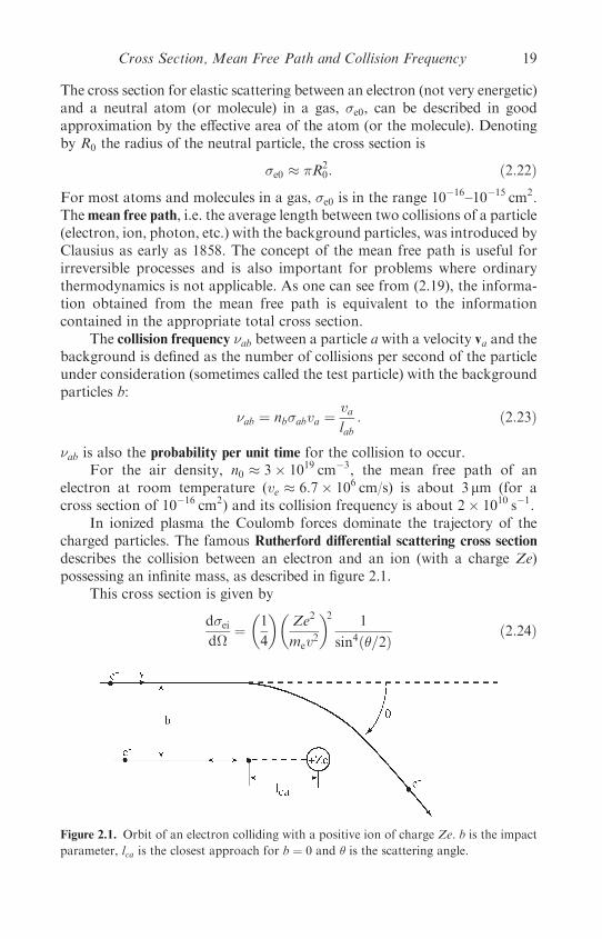
In ionized plasma the Coulomb forces dominate the trajectory of thecharged particles. The famous Rutherford differential scattering cross section

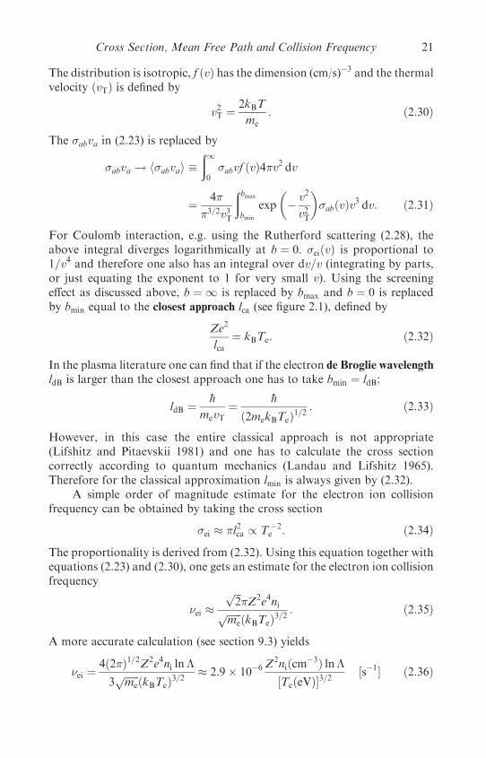
describes the collision between an electron and an ion (with a charge Ze)possessing an infinite mass, as described in figure 2.1.

This cross section is given by

d�eid�

¼�1

4

��Ze2

mev2

�2 1

sin4ð�=2Þð2:24Þ

Figure 2.1. Orbit of an electron colliding with a positive ion of charge Ze. b is the impact

parameter, lca is the closest approach for b ¼ 0 and � is the scattering angle.


where me and v are the mass and the velocity of the electron accordingly, � isthe scattering angle and d� is the differential solid angle. In sphericalcoordinates with an azimuthal symmetry, d� is related to the scatteringangle � by

d� ¼ 2� sin � d�: ð2:25Þ

The impact parameter b, defined asymptotically before the Coulomb interac-tion is effective, is related to the scattering angle � by

b tan�

2¼ Ze2

mev2: ð2:26Þ

Although equations (2.24)–(2.26) are given for an electron–ion collision inthe laboratory system of reference, these equations are also valid for the colli-sion of any two charged particles with masses m1 and m2 and charges q1 andq2 appropriately. For this general collision the following changes are to bedone in the above equations to be valid in the centre of mass:

(a) �Ze2 is replaced by q1q2.(b) The electron mass is replaced by the reduced mass mr defined by

1

mr

¼ 1

m1

þ 1

m2

: ð2:27Þ

(c) v is the relative velocity between the colliding particles.(d) The scattering angle � is given in the centre of mass of the colliding

particles.

The (total) cross section �ei is defined by

�ei ¼ðd�

d�eid�

¼ �

2

�Ze2

mev2

�2 ð�0d�

sin �

sin4ð�=2Þ: ð2:28Þ

The above integral diverges at � ¼ 0, or equivalently (using equation (2.26))for b ! 1. However, the very distant interactions are screened by thesurrounding charged particles so that there is an effective bmax instead ofb ! 1. In general bmax is taken as the Debye length (section 2.4).

In calculating the collision frequency in (2.23) for electron–ioncollisions, one has to take into account the velocity distribution of theparticles, i.e. �abva has to be replaced by h�abvai, an average over all possiblevelocities. For ions at rest and electrons in LTE (for Ti ¼ 0 and an electrontemperature Te), the electron velocity distribution f (v) is given by theMaxwell distribution,

f ðvÞ ¼ 1

ð ffiffiffi�

pvTÞ3

exp

�� v2

v2T

�;

ð10

dv4�v2

ð ffiffiffi�

pvTÞ3

exp

�� v2

v2T

�¼ 1: ð2:29Þ


The distribution is isotropic, f ðvÞ has the dimension (cm/s)�3 and the thermalvelocity ðvTÞ is defined by

v2T ¼ 2kBT

me

: ð2:30Þ

The �abva in (2.23) is replaced by

�abva ! h�abvai �ð10�abvf ðvÞ4�v2 dv

¼ 4�

�3=2v3T

ðbmax

bmin

exp

�� v2

v2T

��abðvÞv3 dv: ð2:31Þ

For Coulomb interaction, e.g. using the Rutherford scattering (2.28), theabove integral diverges logarithmically at b ¼ 0. �eiðvÞ is proportional to1=v4 and therefore one also has an integral over dv=v (integrating by parts,or just equating the exponent to 1 for very small v). Using the screeningeffect as discussed above, b ¼ 1 is replaced by bmax and b ¼ 0 is replacedby bmin equal to the closest approach lca (see figure 2.1), defined by

Ze2

lca¼ kBTe: ð2:32Þ

In the plasma literature one can find that if the electron de Broglie wavelength

ldB is larger than the closest approach one has to take bmin ¼ ldB:

ldB ¼ �h

mevT¼ �h

ð2mekBTeÞ1=2: ð2:33Þ

However, in this case the entire classical approach is not appropriate(Lifshitz and Pitaevskii 1981) and one has to calculate the cross sectioncorrectly according to quantum mechanics (Landau and Lifshitz 1965).Therefore for the classical approximation lmin is always given by (2.32).

A simple order of magnitude estimate for the electron ion collisionfrequency can be obtained by taking the cross section

�ei � �l2ca / T �2e : ð2:34Þ

The proportionality is derived from (2.32). Using this equation together withequations (2.23) and (2.30), one gets an estimate for the electron ion collisionfrequency

�ei �ffiffiffi2

p�Z2e4niffiffiffiffiffiffi

mep ðkBTeÞ3=2

: ð2:35Þ

A more accurate calculation (see section 9.3) yields

�ei ¼4ð2�Þ1=2Z2e4ni ln�

3ffiffiffiffiffiffime

p ðkBTeÞ3=2� 2:9� 10�6 Z

2niðcm�3Þ ln�½TeðeVÞ�3=2

½s�1� ð2:36Þ


� ¼ bmax

bmin

: ð2:37Þ

In the right-hand side of (2.36), ni is the ion density in cm�3 and Te(eV) is theelectron temperature in electronvolt (eV).

2.3 Transport Coefficients

2.3.1 Electrical conductivity

TheDrude model is used to get a simple estimate on the electrical conductivityof a plasma gas. The same formalism is a good approximation for solids(Ashcroft and Mermin 1976). The definition of the electrical conductivityis given by

je ¼ �neeve ¼ �EE ð2:38Þ

where ve is the electron velocity, je is the electric current, ne is the electrondensity and �E is the electric conductivity. The relation between the electriccurrent and the electric field is known as Ohm’s law. Due to the local electricfield E, assumed constant (d.c.) in this model, an electron is acceleratedbetween any two collisions with the background particles. Newton’s lawyields

dvedt

¼ � eE

me

: ð2:39Þ

It is assumed that the collisions are instantaneous and suddenly alter theelectron velocity. In this picture the electrons are bumping from particle toparticle. Denoting by t the time that passed since the last collision of theelectron, the solution of (2.39) is vðt¼0Þ � eEt=me. Since in this model anelectron emerges from a collision in a random direction, vðt¼0Þ does notcontribute to the average velocity. Therefore, assuming that the averagetime between collisions is the relaxation time , the velocity in (2.38) is

ve ¼ � eE

me

; ¼ 1

�ei: ð2:40Þ

An electron in the plasma collides with the ions, the other electrons and if theplasma is not fully ionized it collides also with the neutral atoms. In equation(2.40) it is assumed that this frequency is dominated by electron–ioncollisions. Substituting the velocity from (2.40) into (2.38) one gets theelectrical conductivity

�E ¼ nee2

me�eið2:41Þ


where �E is in s�1 in c.g.s. units, (�m)�1 in m.k.s. (standard units) and therelation between the units is: 1 (�m)�1 ¼ 9� 109 s�1. Using equation(2.36), in (2.41) the electrical conductivity can be written as

�EðeiÞ ¼ 2:7� 1017Z

�Te

keV

�3=2½s�1� ð2:42Þ

where the electron temperature is in keV. It is worthwhile to compare thisnumerical result (equation (2.42)) with the conductivity of a very goodconductor such as copper, �EðcopperÞ ¼ 5:5� 1017 s�1.

For comparison between plasma (known as a good conductor) and a gas(known as a very bad conductor), it is interesting to calculate the d.c. electricalconductivity of air. The first question is how many free electrons are inair at standard conditions. Using the Saha equation (2.16) one getsne � expð�I=ð2TðeVÞÞÞ; I � 15 eV and the room temperature is T � 1=40 eV,therefore the exponential factor is exp(�300), implying practically a zerone. However, due to cosmic radiation the number of induced electrons is ofthe order � 1

2(statcoulomb)/(year cm3)� 30 electrons/(cm3 s) (this numberchanges for different locations on Earth). These free electrons are attachedto the air molecules; taking a lifetime of about 10ns for these electrons, onegets a steady state number of free electrons about ne � 3� 10�7 cm�3.Using this electron density, the electron cross section for colliding with aneutral molecule (2.22), and using the collision frequency (2.23), in (2.41)one gets �EðairÞ � 3� 10�9 s�1, a number that is about 26 orders of magni-tude smaller than the electrical conductivity of copper.

2.3.2 Thermal conductivity

Consider a medium in which the temperature is not uniform, i.e. T is a func-tion of space T ¼ T(r). The tendency to reach equilibrium requires a flow ofheat from the region of higher temperature to that of lower temperature.Defining qH as the energy crossing a unit area per unit time in the directionorthogonal to this area, the heat flux (in erg/(cm2 s)) can be defined by

qH ¼ �rT : ð2:43Þ

The value of can be easily estimated in a simple model. We assume that thetemperature is a function of x, the particles have an average energy "ðxÞ, adensity n and a velocity v. This simplification does not affect the calculationssince does not depend on the model that is calculated. The flux of theparticles in the þx direction, normal to the y–z plane, is 1

6 ðnvÞ (the factor 16

can be understood by considering three dimensions x–y–z and each dimen-sion has two directions). The heat flux qHðxÞ in the direction of þx is

qH ¼ 1

6ðnvÞ½"ðx� lÞ � "ðxþ lÞ� � � 1

3nvl

@"

@x¼ � 1

3nvl

@"

@T

@T

@xð2:44Þ

Transport Coefficients 23

where l is the mean free path discussed in the previous section. Since theenergy derivative with respect to the temperature is the heat capacity (atconstant volume for a process that the density is constant), one gets

qH ¼ � 1

3nvlcV

@T

@x: ð2:45Þ

l is the mean free path of the particles that are transporting the heat (forexample, the molecules in a gas and the electrons in a plasma), cV is theheat capacity per particle at constant volume, and assuming that v equalsthe thermal velocity vT, one gets

¼ 1

3ncVlvT ¼ necVev

2T

3�ei/ T

5=2e ½erg=ðcm s KÞ�: ð2:46Þ

The second equality was obtained using (2.23). For the last proportionalityit was assumed that the electrons are transporting the heat, �ei � Te

�3=2,v2T � Te, and taking for the plasma under consideration a constant cV.

It is worth mentioning that the heat transport in a gas is done by the gasmolecules; and in this case (to a first approximation) the cross section istemperature-independent, the collision frequency is proportional to thetemperature square root, and therefore

ðgasÞ / T1=2 ð2:47Þ

where T is the gas temperature.Comparing the electrical conductivity �E, equation (2.41), with the

thermal conductivity (2.46) and using the ideal gas equation of state(Eliezer et al. 1986), cV ¼ 3

2 kB and (2.30) we get theWiedemann and Franz law

�E¼ 3

2

�kBe

�2T : ð2:48Þ

2.3.3 Diffusion

In equilibrium the electrons are distributed uniformly throughout the plasmaso that ne is independent of position. Suppose that a disturbance causes theelectron density to depend on position ne(r). In this case the electrons willmove in such a way as to restore equilibrium. This motion is described bythe diffusion equation

@ne@t

¼ r ðDrneÞ ð2:49Þ

where D is the diffusion coefficient, defined by the relation

jn ¼ �Drn: ð2:50Þ

jn ¼ nv is the particle current density.


The diffusion coefficient can be calculated using the simple model usedabove (to calculate the thermal conductivity coefficient). The density is a func-tion of one space dimension, nðxÞ, and the particle flux in the þx direction is

jn ¼ 1

6½vTneðx� lÞ � vTneðxþ lÞ� � � 1

3vTl

@ne@x

: ð2:51Þ

The right-hand side of the equation was obtained by the first-order Taylorexpansion. From this equation the diffusion coefficient is

D ¼ 1

3vTl /

T5=2e

ne½cm2=s�: ð2:52Þ

In the presence of a magnetic field in a fully ionized plasma the diffusion coef-ficient in a direction perpendicular to the magnetic field, D?, is a function ofthe magnetic field. In this case, for a steady-state plasma the Ohm law (2.38)(in c.g.s. units) is generalized to

j ¼ �E

�Eþ v� B

c

�ð2:53Þ

where c is the speed of light. The magnetic force (force/volume) J� B=c isbalanced by the pressure gradient (force/volume) rP

j� B

c¼ rP: ð2:54Þ

The plasma velocity in the perpendicular direction to the magnetic field isobtained by taking the cross-product of the generalized Ohm’s law withthe magnetic field [(2.53)�B] and using (2.54) for an ideal gas pressurewith constant temperature, rP ¼ kBTrn. The derived perpendicularvelocity v? is

v? ¼ cE� B

B2� c2kBT

�EB2rn � vdrift þ vdiffusion: ð2:55Þ

Therefore, the diffusion coefficient D? is (�nvdiffusion=rn)

D? ¼ c2nkBT

�EB2

½cm2=s�: ð2:56Þ

This value for D? is known as the classical diffusion. However, it appeared inmany experiments that the 1/B2 scaling law of D? is not satisfied and insteada 1=B dependence was derived (Bohm et al 1949). Bohm, Burhop andMassey, who were using an arc discharge in the presence of a magneticfield for uranium isotope separation, first noted this anomalous diffusion in1946. Bohm suggested the semi-empirical formula

D? ¼ ckBTe

16eB� DB ½cm2=s�: ð2:57Þ

Transport Coefficients 25

The diffusion following this law is called the Bohm diffusion. Note that DB,unlikeD?, does not depend on the density. It was found that (2.57) is satisfiedin a surprisingly large number of experiments.

2.3.4 Viscosity

The pressure is in general a tensor Pij , the first index designating the orienta-tion of the plane and the second index the component of the force exertedacross this plane. In Cartesian coordinates, i or j is equal to x, y, z. Viscosityarises when adjacent fluid elements flowing with different velocities exchangemomentum. The tensor Pij is given by

Pij ¼ P�ij þ �vivj � �

�@vi@xj

þ@vj@xi

� 2

3

X3k¼1

@vk@xk

�ij

�� &

X3k¼1

@vk@xk

�ij: ð2:58Þ

The Navier–Stokes equation of ordinary fluid dynamics can be written in theform (Landau and Lifshitz 1987)

@ð�viÞ@t

¼ �X3k¼1

@Pik

@xk: ð2:59Þ

In general the coefficients of viscosity � (the first coefficient) and � (the secondcoefficient) are positive numbers that are functions of temperature and density.P is the scalar pressure given by the equation of state (Eliezer et al. 1986)

P ¼ Pð�;TÞ ð2:60Þwhere � is the density of the plasma fluid. For an incompressible fluid the diver-gence of the velocity vanishes,r v ¼ 0, and the second coefficient of viscosity� does not contribute to the pressure tensor. In many plasma systems theeffects of viscosity are negligible since the first two terms in (2.58) are muchlarger than the viscous terms. However, we shall estimate the coefficients ofviscosity � in a simple model, as described above for the coefficients of diffu-sion and conductivity. We take an x dependence only and a flow velocityv ¼ ð0; 0; vzÞ, so that the only off-diagonal tensor element of the pressure is

Pxz ¼ �� @vz@x

: ð2:61Þ

Pxz, known as the stress, is the mean increase of the momentum flux in the zdirection transported by the fluid particles per unit time and per unit area inthe x direction (the y–z plane). In this model Pxz is defined by

Pxz ¼ 16 ðnvTÞm½vzðx� lÞ � vzðxþ lÞ� ð2:62Þ

where m is the mass of the particle fluid under consideration. A first-orderTaylor expansion of vz yields

Pxz ¼ ��1

3nmvTl

�@vz@x

� �� @vz@x

: ð2:63Þ


In the calculation of the transport coefficients derived above, the coefficientfactors are not to be taken too seriously. However, the scaling laws with themass m, the mean free path l, the density n and the average velocity (denotedby vT) of the particles under consideration give a reasonable approach for thebehaviour of the transport coefficients: �E, , D and �.

2.4 Radiation Conductivity

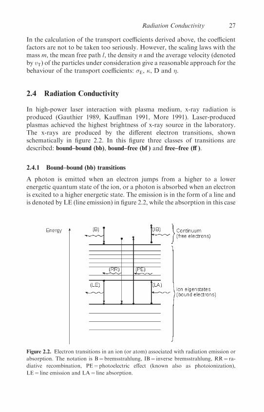
In high-power laser interaction with plasma medium, x-ray radiation isproduced (Gauthier 1989, Kauffman 1991, More 1991). Laser-producedplasmas achieved the highest brightness of x-ray source in the laboratory.The x-rays are produced by the different electron transitions, shownschematically in figure 2.2. In this figure three classes of transitions aredescribed: bound–bound (bb), bound–free (bf ) and free–free (ff ).

2.4.1 Bound–bound (bb) transitions

A photon is emitted when an electron jumps from a higher to a lowerenergetic quantum state of the ion, or a photon is absorbed when an electronis excited to a higher energetic state. The emission is in the form of a line andis denoted by LE (line emission) in figure 2.2, while the absorption in this case

Figure 2.2. Electron transitions in an ion (or atom) associated with radiation emission or

absorption. The notation is B¼ bremsstrahlung, IB¼ inverse bremsstrahlung, RR¼ ra-

diative recombination, PE¼ photoelectric effect (known also as photoionization),

LE¼ line emission and LA¼ line absorption.

Radiation Conductivity 27

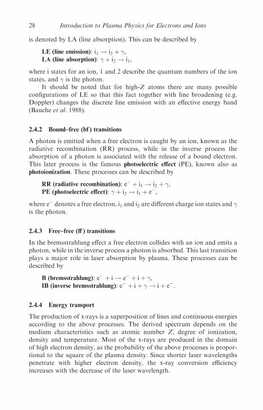
is denoted by LA (line absorption). This can be described by

LE (line emission): i1 ! i2 þ ,LA (line absorption): þ i2 ! i1,

where i states for an ion, 1 and 2 describe the quantum numbers of the ionstates, and is the photon.

It should be noted that for high-Z atoms there are many possibleconfigurations of LE so that this fact together with line broadening (e.g.Doppler) changes the discrete line emission with an effective energy band(Bauche et al. 1988).

2.4.2 Bound–free (bf ) transitions

A photon is emitted when a free electron is caught by an ion, known as theradiative recombination (RR) process, while in the inverse process theabsorption of a photon is associated with the release of a bound electron.This later process is the famous photoelectric effect (PE), known also asphotoionization. These processes can be described by

RR (radiative recombination): e� þ i1 ! i2 þ ,PE (photoelectric effect): þ i2 ! i1 þ e�,

where e� denotes a free electron, i1 and i2 are different charge ion states and is the photon.

2.4.3 Free–free (ff ) transitions

In the bremsstrahlung effect a free electron collides with an ion and emits aphoton, while in the inverse process a photon is absorbed. This last transitionplays a major role in laser absorption by plasma. These processes can bedescribed by

B (bremsstrahlung): e� þ i ! e� þ iþ ,IB (inverse bremsstrahlung): e� þ iþ ! iþ e�.

2.4.4 Energy transport

The production of x-rays is a superposition of lines and continuous energiesaccording to the above processes. The derived spectrum depends on themedium characteristics such as atomic number Z, degree of ionization,density and temperature. Most of the x-rays are produced in the domainof high electron density, as the probability of the above processes is propor-tional to the square of the plasma density. Since shorter laser wavelengthspenetrate with higher electron density, the x-ray conversion efficiencyincreases with the decrease of the laser wavelength.


Detailed studies of the conversion of laser light into x-rays wereperformed for a wide parameter range of laser intensity, wavelength andpulse duration for targets of various atomic numbers. The x-ray generationefficiency (x-ray energy/absorbed laser energy) for soft x-rays, between 0.1 to1 keV of energy, reaches the high value of 80% for a gold target irradiatedwith a 263 nm laser pulse of the order of 1 ns duration.

Since for high-Zmaterials a significant part of the laser energy is convertedinto x-rays, the transport of these x-rays plays an important role in these plasmamedia. In this section the transport of energy by radiation is analysed. Theradiation can be treated classically by electromagnetic fields or quantummechanically by the description of particles called photons. The equation ofradiative transfer can be generally stated as the conservation of a physical quan-tity X (such as the number of photons or the energy density) with a givenfrequency � and direction � in an arbitrary volume V bounded by a closedsurface �. Schematically this statement can be written in the following way:

change of Xð�;�Þ ¼ Xðflow out of volume V via surface �Þ

þ Xðabsorption in the volume VÞ

þ Xðscattering ‘out’ from ð�;�Þ to ð�0;�0Þ within VÞ

þ Xðscattering ‘in’ from ð�0;�0Þ to ð�;�Þ within VÞ:ð2:64Þ

There are many ways to formulate quantitatively this statement of radiationtransport (Zeldovich and Raizer 1966, Pomraning 1973, Mihalas and Mihalas1984, Minguez 1993). We shall follow the simplest approach given byZeldovich and Raizer. For this purpose we introduce a variety of quantitiesusually used to describe the radiation energy transport.

The wavelength � or the frequency � (at which the electromagnetic fieldsoscillate) characterizes the radiation that can also be considered as photonparticles with energy E� and momentum p�. �, �, p� and E� are related bythe Planck constant h and the speed of light c:

� ¼ c

�; E� ¼ h�; p� ¼

h�

c: ð2:65Þ

The distribution function of the photon particles f ([cm�3 s]), where f is afunction of the photon frequency �, the photon position r and direction �at a time t, is described by

f ð�; r;�; tÞ d� d3r d� ¼ number of photons with frequency � at ðr; tÞ ð2:66ÞThe speed of light in the plasma medium is equal to c=nR, where nR is theindex of refraction for photons with a frequency � and is given by

nR ¼�1�

�2pe

�2

�1=2ð2:67Þ


where �pe is the electron oscillation frequency in the plasma. In the domain ofthe critical density, where the incident laser beam is reflected because itcannot penetrate into higher densities, one has for a laser with photonenergy �1 eV and an x-ray photon �100 eV a refractive index nR � 0:99995.Therefore, it is conceivable to assume that in the domain of the criticaldensity and lower densities the x-ray photons move with the speed oflight in vacuum. Hence, one can define the spectral radiation intensity I�[erg/cm2] as the radiation energy per frequency between � and � þ d�,crossing a unit area per unit time in the direction �, within the solid angled�, by

I�ðr;�; tÞ d� d� ¼ h�cf ðr;�; tÞ d� d�; I

�erg

cm2 s

�¼

ðI�ðr;�; tÞ d�:

ð2:68Þ

The radiation field is defined either by f or by I� (both scalar quantities). Twomore useful functions are defined in order to describe the radiation transport,the spectral energy density scalar U� [erg s/cm3] and the spectral energy flux

vector S� [erg s/cm2]

U�ðr; tÞ ¼1

c

ðI� d�; U½erg=cm3� ¼

ð10U�ðr; tÞ d�

S�ðr; tÞ ¼ðI�� d�; S½erg=cm3� ¼

ð10S� r; tð Þ d�;

ðd� ¼ 4�

ð2:69Þ

where � is the unit vector in the direction of the photon motion.In a state of thermodynamic equilibrium, the number of photons in a unit

volume emitted per unit time by the medium in the interval (d�, d�) is equalto the number of absorbed photons in the same interval. The equilibriumradiation field is isotropic and depends only on frequency and the mediumtemperature T . In this case the Planck functions are given for the spectral

radiation intensity I�p [erg/cm2] and the spectral energy density scalar U�p

[erg s/cm3]:

I�p ¼cU�p

4�

U�p ¼�8�h�3

c3

��exp

�h�

kBT

�� 1

��1

Up½erg=cm3� ¼ð10U�p d� ¼

�4�SBc

�T4

�SB ¼ 2�5k4B15h3c2

¼ 5:6705� 10�5 ½ergı=ðcm2 s deg4Þ�

ð2:70Þ


where �SB is the Stefan–Boltzmann constant. The Planck functionU�p, whichdescribes the energy distribution for radiative equilibrium, has a maximum ata photon energy h�max ¼ 2:822kBT . The isotropic equilibrium radiationimplies that the spectral energy flux vector S� is zero. However, it is possibleto define the one-sided spectral energy flux S�p, by integrating I�p cos � (see(2.69) and (2.70)) over a hemisphere, where � is the angle between � andthe flux vector direction:

S�p �ð2�0

d�

ð�=20

d� sin �ðI�p cos �Þ ¼ �I�p ¼cU�p

4

Sp½erg=ðcm2 sÞ� ¼ð10S�p d� ¼ �SBT

4:

ð2:71Þ

Before writing the transport equation, a few more variables have to bedefined. The emissivity j� (erg/cm3) describes the spontaneous emission ofthe medium, and it depends on the medium atoms, the degree of ionizationand the temperature, but it is independent of the existence of radiation.The spontaneous emission is defined by

j� d� d� ¼ [energy/(volume� time)] of spontaneous emission: ð2:72Þ

In order to calculate the total emission of the medium one has to add theinduced emission, given by

j�

�c2I�2h�3

�d� d� ¼ [energy/(volume� time)] of induced emission: ð2:73Þ

The term in the brackets is the number of photons in the same phase spacecell as the emitted photon (with a definite polarization). The total emissionis given by the sum of (2.72) and (2.73).

A transport equation in the form of (2.64) requires the knowledge ofabsorption and scattering. This can be written in the form

�I� d� d� ¼ [energy/(volume� time)] absorbed or scattered

by the medium

� ¼1

l�¼

Xj

nj��j

ð2:74Þ

where � (cm�1) is the opacity (occasionally in the literature, the value

�=� (cm2/g) where � ¼ density is defined as the opacity), the appropriate

mean free path is l� (cm), nj (cm�3) is the density of particles of type j and

��j is the appropriate cross section for absorption or scattering of theprocesses under consideration, as described in figure 2.2. For example


(More 1991), the inverse bremsstrahlung cross-section is given by

�IBff �ð Þ ¼�28��

3ffiffiffi3

p�ðnea3BÞ

�IHkBT

�1=2�IHh�

�3Z2

i a2B

� � 2�e2

hcffi 1

137:036

aB � h2

4�e2me

ffi 0:529� 10�8 cm

IH � e2

2aBffi 13:6 eV

ð2:75Þ

where Zi is the effective ion charge. For h� ¼ kBT ¼ 100 eV andne ¼ 1020 cm�3 one gets a cross section of 4:34� 10�25Z2

i (cm2).

For a hydrogen-like atom the photoelectric cross-section is given by(Zeldovich and Raizer 1966)

�PEbf ð�Þ ¼

�64�4emeZ

4i

3ffiffiffi3

ph6cn5

�1

�3� 7:9� 10�18

�n

Z2i

��Inh�

�3½cm2�

0

for h� > In

for h� < In

8><>:

ð2:76Þ

where In � IH=n2 and n is the quantum level of the electron.

Finally, combining equations (2.72), (2.73) and (2.74) with ‘the change’(in an equation like (2.64)) given by the total derivative of the intensity withrespect to time, one gets the transport equation

1

c

�@I�@t

þ c� rI�

�¼ j�

�1þ c2I�

2h�3

�� I�: ð2:77Þ

Since the value of j� does not depend on the character of the radiation, butis a property of the medium under consideration, one can estimate thisquantity in a thermal equilibrium system. In thermal equilibrium the ratioof the spontaneous emission to the absorption is a universal function ofthe frequency and temperature and is given by (see section 1.1)

j��

¼ 2h�3

c2exp

�� h�

kBT

�¼ I�p

�1� exp

�� h�

kBT

��

j� ¼ 0�I�p

0� � �

�1� exp

�� h�

kBT

��:

ð2:78Þ

Equation (2.78), known as Kirchhoff’s law, is based on the general law ofdetailed balance between emission and absorption of a physical process,


where T is the temperature of the medium. For this equation to be valid, it isnot mandatory for the radiation to be in equilibrium with the matter, but it isrequired that a local temperature can be defined for the atoms and ions of themedium.

Substituting (2.70) into (2.78), one finds that the right-hand side of(2.77) equals j� � �f1� exp½�h�=ðkBTÞ�gI�. Using again the relations(2.78), the transport equation (2.77) can be rewritten as

@I�c @t

þ � rI� ¼ 0�ðI�p � I�Þ: ð2:79Þ

Integrating this equation over the solid angle and using the relations (2.69)and (2.71), one gets another equivalent form of the transport equation

@U�

@tþr S� ¼ c0�ðU�p �U�Þ: ð2:80Þ

This transport equation describes the radiation energy conservation of afrequency �. In order to use this equation the matter of the mediumshould be in local thermodynamic equilibrium (LTE).

2.5 Debye Length

In plasma the Coulomb interaction range is reduced due to the screening

effect. In order to calculate the screening scale length, called the Debyelength and denoted by �D, imagine a charge Ze at rest at the origin of thecoordinates surrounded by plasma electrons. The vector position fromthe ion is given by r. The plasma system is neutral, i.e. one can look atthe ions as a neutralizing background for the plasma electrons having atemperature Te.

The equation of motion of the electron fluid in this case is given by

neeEþrPe ¼ 0 ð2:81Þ

where E is the electric field and Pe the electronic pressure. Assuming an idealgas equation of state

Pe ¼ nekBTe ð2:82Þ

with a constant electron temperature, Te, and defining the electrostaticpotential ’, E ¼ �r’, one gets from the electron equation of motion (2.81)

neer’ ¼ kBTerne ð2:83Þ

the following electron distribution

ne ¼ n0e exp

�e’

kBTe

�ð2:84Þ

Debye Length 33

where n0e is initial uniform density of the electrons. The electron potential ’is obtained by solving the Poisson equation (in c.g.s. units):

r2’ ¼ �4�Ze�ðrÞ þ 4�eðne � n0eÞ ð2:85Þ

where �(r) is the Dirac function and it takes care that for r ! 0, ’! Ze=r.Substituting (2.84) into (2.85) and expanding the exponential for

e’=ðkBTeÞ � 1, one gets the differential equation�r2 � 1

�2De

�’þ 4�Ze �ðrÞ ¼ 0 ð2:86Þ

where the electron Debye length �De is

�De ¼�

kBTe

4�e2n0e

�1=2� 743

�TeðeVÞ

n0eðcm�3Þ

�1=2: ð2:87Þ

The solution of equation (2.86) is

’ ¼ Ze

rexp

�� r

�De

�: ð2:88Þ

This solution shows that the screening effect, namely the Coulomb interac-tion 1=r law of the electrostatic potential, is changed according to equation(2.88), implying that the effective infinite range of the Coulomb interactionis shortened to a distance of the order of �De.

At this stage let us compare the characteristic lengths of a plasmamedium with the Debye length �De. In discussing the binary collisionsbetween charged particles, the closest approach was introduced, i.e. (2.32).For an ion with a charge Z ¼ 1 one has

lcaðcmÞ � 1:44� 10�7

TðeVÞ : ð2:89Þ

The cross section for close collisions between charged particles is of the orderof �l2ca; therefore the mean free path l, equation (2.19), is of the order of

lðcmÞ ¼ 1

n�¼ 1

n�l2ca� 4:89� 1012

TðeVÞ2

nðcm�3Þ: ð2:90Þ

Taking the scale of length as the average distance between charged particles,a0 ¼ n�1=3, we get

�De

a0� 0:29

�lcaa0

��1=2

� 0:50

�l

a0

�1=4: ð2:91Þ

For example, for a laser plasma interaction with n ¼ 1021 cm�3, T ¼ 100 eV,one gets a0 ¼ 10:0� 10�8 cm, �D=a0 ¼ 2:37, lca=a0 ¼ 0:014 and l=a0 ¼ 490,so that in this case l > �D > a0 > lca.


Another scale length is introduced by the gyro motion of chargedparticles in the presence of a magnetic field B. The electron gyroradius re,known as the Larmor radius, is given by

re ¼mevec

eB� 2:38

TeðeVÞ1=2

BðgaussÞ ½cm�: ð2:92Þ

The evaluation of the right-hand side of (2.92) was done with ve equal to thethermal velocity. In the above numerical example, the gyroradius re is of theorder of the mean free path l for a magnetic field of about 0.5megagauss(MG), a value achieved easily in laser plasma interactions. For re to beequal to the Debye length, a magnetic field of 100MG is needed.

Assume that, in a plasma with dimension L large in comparison to �De,a local charge fluctuation is created or an external potential is introduced.In this case the created electric fields are shielded for a distance smallerthan L. However, within dimensions of the order of �De the plasma is notneutral and the electric forces do not vanish there, although the plasma isneutral on the large scale, L � �De. This situation is described by sayingthat the plasma is quasineutral.

The Debye shielding is effective only if the number of electrons in thecloud surrounding the ion is large enough. If on average there are only oneor two electrons in a sphere with a radius �De, known as a Debye sphere,then the Debye shielding is not a statistically valid concept. Therefore,defining the number of electrons, NDe, in a sphere with a radius �De by

NDe ¼ 43�ne�

3De ð2:93Þ

the effective Debye shielding requires NDe � 1. NDe is usually called theplasma parameter.

For example, in a typical plasma created in laser solid interaction withan electron temperature of 1 keV and an electron density of 1021 cm�3, onehas �De ¼ 7:5� 10�8 cm and NDe ¼ 170. Note that the typical laser wave-length �L, of the order of 1 mm, is about 103 larger than �De.

For plasmas where the ion temperature, Ti, is not zero the ions alsocontribute to the Debye shielding. The ion fluid equation of motion, similarto equation (2.81), is

ZeniE�rPi ¼ 0 ð2:94Þ

and the ion pressure, Pi, is given by the ideal gas equation of state

Pi ¼ nikBTi: ð2:95Þ

Similarly, to the derivation of (2.84) for the ion distribution; one gets

ni ¼ ni0 exp

�� Ze’

kBTi

�: ð2:96Þ

Debye Length 35

The initial uniform ion density ni0 is related to the electron undisturbeddensity ne0 by

ne0 ¼ Zni0: ð2:97Þ

Instead of (2.86), the Poisson equation (2.85) yields the equation�r2 � 1

�2De

� 1

�2Di

�’þ 4�Ze�ðrÞ ¼ 0 ð2:98Þ

where Ze’=ðkBTeÞ � 1 has been assumed and the ion Debye length isdefined by

�Di ¼�

kBTi

4�e2ni0

�1=2: ð2:99Þ

In the solution of the Poisson equation (2.88) one has to substitute �De with�D defined by

1

�2D¼ 1

�2De

þ 1

�2Di

: ð2:100Þ

2.6 Plasma Oscillations and Electron Plasma Waves

In this section the equations describing the plasma oscillations and theelectron plasma waves are derived from a set of very simple equations,based on the hydrodynamic theory without a magnetic field in the plasma.The plasma is assumed to be cold, that is, the plasma temperature is zero,and therefore the thermal velocities of the electrons and the ions vanish. Inhydrodynamic theory this means that no pressure forces exist in theplasma. Also, as is usually done with the simplest models, it is assumedthat the ions are a stationary background of charge which neutralizes theunperturbed plasma at each point. In this case a perturbation is applied inspace only to the electrons and due to this disturbance an electric field iscreated in the plasma. The question is how the electrons move in this case.

Although the mathematics of this model are quite simple, the solutionillustrates a general behaviour of the plasma. For this problem the followingMaxwell equation is of interest (in c.g.s.):

r E ¼ 4��e ð2:101Þ

where �e is the electric charge density related to the local current densityje, given in (2.38). The equation of charge conservation is given by (seeappendix A)

r je þ@�e@t

¼ 0: ð2:102Þ


Substituting into (2.102) the density current from (2.38), taking the timederivative of this equation and using (2.101), one gets the following equationfor �e:

@2�e@t2

þ�4�e2neme

��e ¼ 0: ð2:103Þ

The quantity in the brackets of (2.103) has the dimensions of the square of anangular frequency known as the plasma frequency !pe:

!pe ¼�4�e2neme

�1=2� 5:64� 104

ffiffiffiffiffine

p ðrad=sÞ ð2:104Þ

where the electron density ne is given in cm�3. This result can be easily under-stood in one dimension by considering a slab of plasma. A perturbation is setup to displace the electrons through a small distance x in a direction normalto the slab, while the positive ions are fixed and at rest (i.e. assuming aninfinite mass for the positive ions). This translation of the electrons inducesan effective surface charge density þneex on the faces of the original slaband�neex on the faces of the shifted electrons. The charge separation createsa uniform electric field equal to 4�enex that applies a restoring force on eachelectron. Newton’s law of motion gives a simple harmonic motion of theelectrons at the plasma frequency. From this picture one can conclude thatthe mechanism of plasma oscillations is an expression of the plasma topreserve its electrical neutrality.

Equation (2.103) does not describe a wave, that is, the oscillations donot propagate. In order to get a wave the plasma should have a nonzerotemperature. We shall analyse the case where the electrons have a tempera-ture Te and the ions are at rest, i.e. Ti ¼ 0. The two hydrodynamic equationsin this case are the mass conservation

@ne@t

þr ðneveÞ ¼ 0 ð2:105Þ

and the momentum conservation

mene

�@ve@t

þ ðve rÞve�¼ �eneE�rPe ð2:106Þ

where ne and ve are the electron density and velocity respectively, �e and me

are the appropriate charge and mass of the electron, E is the electric field inthe plasma and Pe is the electronic pressure. The relation between thepressure and the temperature is known as the equation of state. The idealgas equation of state for the electrons in the plasma is

Pe ¼ nekBTe: ð2:107Þ

Plasma Oscillations and Electron Plasma Waves 37

Moreover, an isentropic (constant entropy) equation for the ideal gas isassumed with constant specific heats and a constant number of electrons

Pe ¼ Cn e ð2:108Þ

where C is a function of the entropy and is constant for the isentropicprocess. The adiabatic exponent is defined by

¼ cPcV

¼ gþ 2

gð2:109Þ

where cP and cV are the specific heats at constant pressure and volume respec-tively and g is the number of degrees of freedom. In one dimension ¼ 3(g ¼ 1) while in three dimensions ¼ 5=3 (g ¼ 3) for free moving particles.From (2.107) and (2.108) one gets

rPe ¼ Pe

�rnene

�¼ kBTerne: ð2:110Þ

Equations (2.106), (2.107) and (2.110) are to be solved together with theMaxwell equation

r E ¼ 4�eðni � neÞ: ð2:111Þ

These equations are nonlinear and therefore it is not easy to get a solution inthe general case. However, if all the amplitudes of oscillations are small andhigher-order terms of the amplitude factors can be neglected, then the equa-tions can be easily solved by the procedure of linearization. We denote theequilibrium part by a subscript 0 and the oscillating amplitudes by thesubscript 1:

ne ¼ ne0 þ ne1; ve ¼ ve0 þ ve1; E ¼ E0 þ E1: ð2:112Þ

The equilibrium conditions for the simple model discussed here is

ne0 ¼ ni ¼ const:; ve0 ¼ 0; E0 ¼ 0;@

@tfne0; ve0;E0g ¼ 0: ð2:113Þ

As already mentioned, the linearization approach requires (ne1=ne0Þ2 �ðne1=ne0Þ, ðve1 rÞve1 � @ve1=@t, etc., therefore reducing equations (2.105),(2.106), (2.110) and (2.111) to

@ne1@t

þ ne0r ve1 ¼ 0

me

@ve1@t

¼ �eE1 � kBTerne1;

r E1 ¼ �4�ene1:

ð2:114Þ

For further simplicity a one-dimension model is assumed so that all variablesare functions of time t and space x, and the adiabatic exponent is ¼ 3.


Substituting a monochromatic wave solution with a frequency ! and a wave

number k ¼ 2�=� where � is the wavelength

ne1 ¼ n exp½iðkx� !tÞ�

ve1 ¼ v exp½iðkx� !tÞ�

E1 ¼ E exp½iðkx� !tÞ�

ð2:115Þ

into (2.114), a set of linear algebraic equations is obtained

!n� ne0kv ¼ 0

�i!mevþ eE þ 3ikkBTen ¼ 0

ikE þ 4�en ¼ 0:

ð2:116Þ

The solution of (2.116) is the following dispersion relation for the electronplasma wave, known also as a plasmon:

!2 ¼ !2p þ 3k2v2th: ð2:117Þ

The thermal velocity vth in the one-dimension model is

vth ¼

ffiffiffiffiffiffiffiffiffiffikBTe

me

s: ð2:118Þ

The two velocities related to the wave, the phase velocity v� and the groupvelocity vg (the velocity that energy is transferred), defined by

v� ¼ !

k; vg ¼

d!

dkð2:119Þ

are connected to the thermal velocity by the dispersion relation (2.117)

vgv� ¼ 6v2th: ð2:120Þ

Laser light can interact directly with the plasma particles and also with theplasma waves (Kruer 1988, Liu and Tripathi 1995). The plasma waves maybe of an electromagnetic nature, i.e. transverse waves, or of an electrostaticor acoustic nature, i.e. longitudinal waves, like the one described above (theplasmon).

In the presence of magnetic fields a large zoo of plasma waves are possible(Stix 1992).

In a plasma state of equilibrium it is important to know what happens ifone of the plasma parameters is slightly disturbed. If the disturbance grows,the plasma is unstable, while if the small disturbance decays and disappears,the plasma is in a stable equilibrium. Plasma instabilities are classified in twolarge categories: macroinstabilities are associated with a departure fromequilibrium of a large part of the plasma system, and microinstabilities are

Plasma Oscillations and Electron Plasma Waves 39

associated with small disturbances in the velocity of the plasma particles,which can increase and cause the plasma to be unstable.

It is worth mentioning some of the colourful descriptive names givento plasma wave instabilities: sausage, kink, banana, firehose, flute, inter-change, two-stream, tearing, loss-cone, mirror, ion-acoustic, Brillouin,Raman, parametric, two-plasmon, Rayleigh–Taylor, Richtmyer–Meshkov,Kelvin–Helmholtz, etc. We shall encounter some of these instabilities (inbold letters) in the following chapters.

Every wave has its own dispersion relation, namely a relation betweenthe wave number k and the frequency ! described by some functionFð!; kÞ ¼ 0. Denoting the plasma wave amplitude for any parameter (suchas density, temperature, electric field, magnetic field, pressure, etc.) by ,one can write

/ exp½iðkx� !tÞ�: ð2:121Þ

There are two ways to analyse the different domains of the dispersion relationin !–k space:

(a) The wave instability in time at a given x. The solution of the disper-sion relation Fð!; kÞ ¼ 0 may yield a complex frequency ! ¼ !R þ i!I, where!R and !I are the real and imaginary values of !. If !2 < 0 then !I 6¼ 0, andfrom (2.121) one gets

/ expð!ItÞ: ð2:122Þ

For t ! 1 the amplitude goes to infinity for !I > 0, namely the domain in!–k space where !I > 0 is unstable, and if the wave is ‘allowed’ to be there bythe dispersion relation then we get an instability.

The nonzero imaginary part of the frequency, !I, plays an importantrole in the physical phenomenon of collisionless damping, known also asLandau damping. This effect describes the damping of a plasma wave as itpropagates away from its point of origination, even though there are nobinary collisions in the plasma.

(b) If instead we want to know how a disturbance develops in space fora fixed frequency, then one must solve Fð!; kÞ ¼ 0 for k in terms of !.A complex k ¼ kR þ ikI implies

/ expð�kIxÞ ð2:123Þ

and for a very large plasma system with kI < 0 the amplitude goes toinfinity for x ! 1, and an instability arises.

2.7 The Dielectric Function

In this section it is shown that the plasma medium can also be described as adielectric medium with a scalar function ". In the general case " is a tensor.


The Maxwell equations are summarized in Appendix A. The plasma isdescribed there as a vacuum with electromagnetic sources, given by theelectric charge density �e and electric current density Je. In Gaussian unitsthe two Maxwell equations that include the sources are

r E ¼ 4��e; r B ¼ 1

c

@E

@tþ 4�

cJe: ð2:124Þ

These equations are equivalent to the following two equations of a dielectricmedium:

r "Eð Þ ¼ 0; r B ¼ 1

c

@ "Eð Þ@t

: ð2:125Þ

The other two Maxwell equations are identical in vacuum and in a dielectricmedium. For simplicity we shall prove the equivalence of equations (2.124)and (2.125) for the following sources:

�e ¼ �ene þ qn0; Je ¼ �eneve: ð2:126Þ

Equations (2.126) assume that the ions are stationary and serve as a charge-neutralizing background (i.e. qn0 ¼ constant) to the electron motion. More-over, we assume a monochromatic electromagnetic field

Eðr; tÞ ¼ EðrÞ expð�i!tÞ; Bðr; tÞ ¼ BðrÞ expð�i!tÞ: ð2:127Þ

The electron velocity ve in the electric current is calculated from Newton’slaw:

@ve@t

þ �eve ¼ � e

me

EðrÞ expð�i!tÞ ð2:128Þ

where �e is the electron collision frequency, for example the electron–ioncollision frequency. The solution of (2.128) for constant �e is

veðr; tÞ ¼�ieEðr; tÞmeð!þ i�eÞ

: ð2:129Þ

Substituting this solution into the electric current density (2.126), one gets

Jeðr; tÞ ¼ �EEðr; tÞ; �E ¼i!2

pe

4�ð!þ i�eÞð2:130Þ

where �E is the (complex) electrical conductivity and !pe is the plasmaangular frequency as defined in (2.104). Substituting Je and using@=@t ¼ �i! (note that this relation is correct only for linear equations)into the second equation of (2.124), one gets the second equation of(2.125) if the dielectric function of the plasma medium is defined by

" ¼ 1�!2pe

!ð!þ i�Þ ¼ 1þ i4��E!

: ð2:131Þ

The Dielectric Function 41

The proof of the equivalence of the first equation of (2.124) and (2.125) isgiven as

r ð"EÞ ¼ r Eþr ½ð"� 1ÞE� ¼ 4��e þr ½ð"� 1ÞE�

¼ 4��e �4�e2

!ð!þ i�eÞme

r neEð Þ ¼ 4��e �4�

i!r �eneveð Þ

¼ 4��e �4�

i!r Je ¼ � 4�

i!

�@�e@t

þr Je�

¼ 0: ð2:132Þ

In the third equality, equation (2.131) and !2pe / ne were used; the fourth

equality was obtained with the help of equation (2.129); the next equalityuses the current density definition; and the last step is the continuityequation.

In summary, we have seen that a plasma can be described as a dielectricmedium with a dielectric function, as given in equation (2.131) (for theelectromagnetic sources of (2.126)).

Assuming a spatial dependence expðik rÞ for the electric and magneticfields, one gets from Maxwell equations the following dispersion relation forthe electromagnetic field:

k2 ¼ !2"

c2, !2 ¼ !2

pe þ k2c2: ð2:133Þ

In this case, the index of refraction for the electromagnetic wave propagatingin the plasma medium is given by

~nn ¼ffiffiffi"

p¼ ~nnR þ i~nnI: ð2:134Þ

2.8 The Laser-induced Plasma Medium

The purpose of this section is to define some of the nomenclature used in thefollowing chapters and to get some orders of magnitude for the plasma systemsto be discussed. In this book we consider high-power laser irradiation, fromIL � 109 W/cm2 up to IL � 1020 W/cm2, with laser pulse duration betweenL � 10ns and as short as L � 10 fs. Practically, up to about IL�

2L �

1016 (W=cm2)mm2 has been experimentally achieved with the long laserpulse duration ðL � 1 nsÞ, while values as high as IL�

2L � 1020 (W/cm2)mm2

have been achieved with the so-called femtosecond lasers (L between 10and 500 fs).

The maximum electric (Emax) and magnetic (Bmax) fields of the laser invacuum are related to the laser irradiance IL (in Gaussian units) by

IL ¼ cE2max

8�¼ cB2

max

8�ð2:135Þ


and in practical units one has

Emax

��V

cm

��ffi 2:75� 109

�IL

1016 W=cm2

�1=2

Bmax½Gauss� ffi 9:2� 106�

IL

1016 W=cm2

�1=2:

ð2:136Þ

For the long laser pulses a corona is created, while the laser–plasma system isdescribed schematically in figure 2.3. This figure is relevant for the long laserpulses (typically �1 ns). As an order of magnitude for low and high densitiesin figure 2.3, the following values can give an indication about the plasmasystems: absorption domain: density <0.01 g/cm3, temperature �1000 eV (inenergy units); transport domain: density between �0.01 g/cm3 and the solidtarget density �0, temperature �30 eV to 1000 eV; compression domain:density � �0 up to 10�0, temperature �1 eV to 30 eV.

The laser propagates up to the critical density nc, about 1021 cm�3 for a

laser with a wavelength of 1 mm. Note that the critical density is inverselyproportional to the square of the laser wavelength

nc½cm�3� ¼ 1:1� 1021�1 mm�L

�2: ð2:137Þ

Figure 2.3. A schematic description of laser–plasma interaction.

The Laser-induced Plasma Medium 43

The plasma system from the critical density outwards (towards the laserirradiation) is defined as the corona. The electrons in the corona absorbthe laser. The absorbed energy is transported from the critical density tothe area where the plasma is created, defined as the ablation surface infigure 2.3. The blow-off velocity of the plasma (towards the laser) is aboutequal to the sound speed cT (at constant temperature) at the critical density

ublow-off½cm=s� � cT ¼�ZkBTe

mi

�1=2� 3� 107

��Z

A

�1=2� Te

keV

�1=2�ð2:138Þ

and the size of the corona is about few times cTL. Therefore, for the femto-second laser pulses the corona is extremely small, and practically it does notexist. In this case the laser is absorbed in the skin depth � of the solid target

� ¼ c

!p

� 1:68� 10�6

�1023 cm�3

ne

�1=2½cm�: ð2:139Þ

For high laser irradiance, IL�2L > 1014 (W/cm2) mm2, two (or more) types

of electrons are produced: the ‘cold’ electrons, with a temperature Te ofthe order of 1 keV; and the ‘hot’ electrons, with a typical temperatureTH > 10 keV. Occasionally the situation is more complicated since a localthermodynamic equilibrium for the electrons cannot be defined for the twospecies of electrons (‘cold’ and ‘hot’). The ‘cold’ electrons carry energyaway from the point of absorption by the diffusion process (thermal conduc-tion). The ‘hot’ electrons deposit their energy ahead of the thermal conduction

front induced by the ‘cold’ electrons, causing ‘hot’ electron preheating. ForIL�

2L > 1014 (W/cm2) mm2 the transport of energy inside the undisturbed

target seems to be inhibited in comparison with the classical diffusionprocess.

There are a few kinds of pressure in laser produced plasma. First, thelight pressure PL caused by the direct laser radiation

PL ¼ ILcð1þ RÞ � 3:3Mbar

�IL

1016 W=cm2

�ð1þ RÞ ð2:140Þ

where R is the laser reflectivity (0 < R < 1) and c is the speed of light. Onecan see that for very high laser irradiance, of the order of 3� 1018 W/cm2,one can get a radiation pressure of 1Gbar, an extremely high pressure.One of the effects of PL is to steepen the density gradient near the criticaldensity.

The second kind of pressure in the corona is the thermal pressure ofplasma particles: the ‘cold’ electron pressure Pe, the ‘hot’ electron pressure

PH and the ion pressure Pi, associated with the different temperatures Te,TH and Ti accordingly. The two electron temperatures are obtained if theelectrons in the corona have two distinct velocity distributions. To a good


approximation, the ideal gas equations of state may be used, namely

Pe ¼ nekBTe � 1:6Mbar

�ne

1021 cm�3

��Te

keV

�

PH ¼ nHkBTH

Pi ¼ nikBTi:

ð2:141Þ

The third kind of pressure is the ablation pressure Pa associated with theflow of heated plasma from the solid target. The ablation pressure drives ashock wave into the solid target and causes it to compress. The inhibition ofenergy transport and the creation of ‘hot’ electrons reduce the value of theablation pressure. A very important feature related to the ablation pressureis related to hydrodynamic instability. Since the ablation pressure acts bya lower density (hot plasma) on a higher density (cold plasma), theRayleigh–Taylor instability occurs.

Between the critical and the ablation surfaces the plasma might bestrongly coupled. In ideal plasma, like in the corona, the Coulomb inter-actions are weak in comparison with the thermal energy. Defining the ratiobetween the Coulomb and thermal energies by �,

� ¼ Coulomb interaction energy

Thermal interaction energy

)�� > 1 for strongly coupled plasmas

� < 1 for ideal plasmas

�: ð2:142Þ

It is convenient to use the mean spacing between particles by the radius of thesphere that each particle occupies:

ak ¼�

3

4�nk

�1=3; k ¼ e or i: ð2:143Þ

The strongly coupled parameters, �ii for ions (with a charge Ze), �ee for elec-trons and �ei for the electron–ion coupling, can be defined by

�ii ¼Z2e2

aikBTi

; �ee ¼e2

aekBTe

; �ei ¼Ze2

aekBTe

: ð2:144Þ

In ideal plasma, unlike in strongly coupled plasma, a large number ofparticles participate in the screening, namely many particles are in theDebye sphere. In a strongly coupled plasma the electrons are degenerate(like in a solid) so that the Fermi–Dirac distribution describes the electrons,while the ideal electrons in plasma are described by theMaxwell distribution.A good review of strongly coupled plasma can be found in More (1986).

Last but not least, for very high laser irradiances relativistic effects mightbecome important. In the relativistic regime, the relativistic factor is relatedto the quiver energy Eq and the quiver velocity vq of the electrons (in the

The Laser-induced Plasma Medium 45

electromagnetic field of the laser) by

Eq ¼ mec2 ¼ ½ð mevqÞ2c2 þm2

ec4�1=2

vq ¼eEL

me!L

!L ¼ 2��Lc

:

ð2:145Þ

Using (2.135) we get

¼�1þ IL�

2L

�0

�1=2�

�1þ IL�

2L

1:4� 1018 ðW=cm2Þ mm2

�1=2

�0 ¼��

2

�m2

ec5

e2½erg=s�:

ð2:146Þ

Therefore, the relativistic effects for the electrons are important forIL�

2L > 1018 (W/cm2) mm2.


Chapter 3

The Three Approaches to Plasma Physics

There are three basic approaches to plasma physics: the hydrodynamic theory,the kinematic theory and the particle theory. The particle theory approach isusing the equations of motion for the individual plasma particles, and withthe help of particle simulation codes and appropriate averages the plasmaphysics is analysed. The kinematic theory is based on a set of equationsfor the distribution functions of the plasma particles, together with Maxwellequations. In the hydrodynamic model the conservation laws of mass,momentum and energy are coupled to Maxwell equations. In addition, fora fluid model, a local thermodynamic equilibrium is assumed and the knowl-edge of the equations of state (relations between pressure, temperature,energy, entropy, etc.) is mandatory for solving the problem.

3.1 Fluid Equations

3.1.1 Mass conservation

We define �(r, t) as the mass density and u(r, t) its velocity for a mass elementpositioned at r at time t. Denoting the differential volume and surface vectorby dV and dA accordingly, the mass conservation can be written in anintegral form by

@

@t

ð�� dV þ

þS�u � dA ¼ 0: ð3:1Þ

The first term, the change of mass in a volume �, is balanced by the mass flowacross surface S enclosing the volume � (the second term). Using Gauss’theorem, one gets for equation (3.1)

@

@t

ð�� dV þ

ð�r � ð�uÞ dV ¼ 0: ð3:2Þ

47

Since the last relation is true for any arbitrary volume �, one obtains thefollowing equation (known also as the equation of continuity) which describesthe conservation of mass:

@�

@tþr � ð�uÞ ¼ 0: ð3:3Þ

3.1.2 Momentum conservation

It is convenient to consider the frame of reference of a moving volume whosesurface encloses a constant amount of fluid. This fluid mass � dV , called a‘fluid particle’, has a vector velocity u. D/Dt describes the change in time(total derivative) of a moving fluid volume and is related to the partial timederivative by

D

Dt¼ @

@tþ u � r: ð3:4Þ

Denoting the surface forces by a tensor f, with dimension of (force/area), andthe volume forces by a vector F, with dimensions of (force/volume), one canwrite Newton’s second law asð

��Du

DtdV ¼

þSf � dAþ

ð�FdV : ð3:5Þ

Neglecting viscosity, the tensor f is given by

fij ¼ �P�ij ð3:6Þwhere P is the pressure and i; j ¼ 1; 2; 3 denotes three orthogonal directionsin space, e.g. x–y–z directions. The first term on the right-hand side of (3.5)can be transformed into a volume integral by using Gauss’ theorem

þS

X3j¼1

fij dAj ¼ �þSP dAi ¼�

ð�

@P

@xidV : ð3:7Þ

Using this relation in (3.5), one getsð��Du

DtdV ¼ �

ð�rPdV þ

ð�FdV : ð3:8Þ

Since the last equation is satisfied for any arbitrary volume �, the followingdifferential equation is valid:

�Du

Dt¼ �rPþ F: ð3:9Þ

Using (3.4) the momentum conservation equation is derived in the formsuggested by Euler:

�@u

@tþ �ðu � rÞu ¼ �rPþ F: ð3:10Þ

48 The Three Approaches to Plasma Physics

The volume forces F are acting on the fluid and differ from one problem toanother. For example, the electromagnetic force due to the motion of freecharges is equal to (in m.k.s. units)

F ¼ �eEþ J� B ð3:11Þ

where E and B are the electric and magnetic fields respectively, J is the sum ofthe current flow due to the transport of charges and �e is the electric chargedensity. In a similar way, the polarization force, the magnetization force, thegravitational force or any other force acting on the volume elements can betaken into account.

3.1.3 Energy conservation

The energy conservation (units of [energy/second]) in the frame of referenceof the moving fluid element is

ð��Dðu2=2Þ

DtdV þ

ð��D"

DtdV ¼ Qext þQH þWF þWf: ð3:12Þ

The first term and the second term on the left-hand side of the equation arethe rate of change of the kinetic energy and the internal energy accordingly. "is the energy of the fluid per unit mass (energy/mass). The increase of the fluidparticle energy (left-hand side of the equation) is balanced by the externalenergy sources Qext, the heat conduction QH, the work per unit time doneby the volume forces WF, and the surface forces Wf. The rate of workdone by the surface forces is obtained by integrating u � f over the surfaceof the fluid particle. Neglecting viscosity, one gets

Wf ¼þSu � f � dA ¼ �

þSPu � dA ¼ �

ð�r � ðPuÞ dV : ð3:13Þ

Again, Gauss’ theorem was applied in the last equality. The rate of workdone by the volume forces is

WF ¼ð�F � u dV : ð3:14Þ

The energy entering the fluid particle per unit time by heat conduction is

QH ¼ð�qH dV ¼ �

ð�r � ð�rTÞ dV : ð3:15Þ

The rate at which external energy enters the fluid particle depends on thesystem under consideration. In particular for the electric (Ohm) depositionof energy

Qext ¼ð�qext dV ¼

ð�E � JdV : ð3:16Þ

Fluid Equations 49

Substituting (3.13)–(3.16) into (3.12), one gets

�D

Dtð"þ 1

2 u2Þ þ r � ðPuÞ

¼ F � u�r � ð�rTÞ þ E � J�

energy

volume� second

�: ð3:17Þ

Using (3.4), the first term on the left-hand side of (3.17) is

�D

Dtð"þ 1

2 u2Þ ¼ �

@

@tð"þ 1

2 u2Þ þ �u � rð"þ 1

2 u2Þ

¼ @

@tð�"þ 1

2 �u2Þ � ð"þ 1

2 u2Þ @�@t

þr � ½�uð"þ 12 u

2Þ�

� ð"þ 12 u

2Þr � ð�uÞ

¼ @

@t½�ð"þ 1

2 u2Þ� þ r � ½�uð"þ 1

2 u2Þ�: ð3:18Þ

The mass conservation (3.3) was used to obtain the last relation. Substituting(3.18) into (3.17), the differential equation that describes the energy conser-vation is derived in its known form:

@

@t½�ð"þ 1

2 u2Þ� þ r � ½�uð"þ 1

2 u2Þ þ Pu� ¼ F � u�r � ð�rTÞ þ E � J: ð3:19Þ

The differential equations describing a fluid system are: mass conservation

(3.3), momentum conservation (3.10) and the energy conservation (3.19). Forthese equations one has to define initial conditions and boundary values.Moreover, it is necessary to know the relations between �–P–T–", knownas the equations of state. Furthermore, the knowledge of the transportcoefficients such as � is required. Last but not least, for a plasma systemthe fluid equations are coupled to the Maxwell equations (given in AppendixA) since the volume forces F and also the pressure may be a function of theelectromagnetic fields. For the external energy deposition we took the Ohmicheating term, E � J; however, for a laser plasma system this source of energymight need a ‘special treatment’.

The fluid equations for the laser-induced plasma system are given below.We consider the general case where the electron temperature Te is not equalto the ion temperature Ti. The ideal equations of state are taken separatelyfor the ion fluid and the electron fluid, i.e.

Pe ¼ nekBTe; Pi ¼ nikBTi

Ee ¼ 32 nekBTe; Ei ¼ 3

2 nikBTi

ð3:20Þ

where me, mi and ve, vi are the masses and the velocities of the electron andthe ion accordingly, and nj and Ej ( j ¼ e or i) are the particle and the energydensities. The fluid equations (3.3), (3.10) and (3.19) for the electrons and the


ions are obtained by using the definitions of the densities �j ¼ mjnj and"j ¼ Ej=�j for j ¼ e or i for the ideal equations of state.

Moreover, the following assumptions are used in deriving the two fluidenergy equations:

(a) The electron fluid is coupled to the ion fluid through the electron–ioncollisions described by the term �(Te � Ti).

(b) The volume force is given only by the electric field in the plasma E.(c) As usually happens the external source term (energy/(volume � time)),

denoted by qL, contributes only to the electron fluid, i.e. the electronsabsorb the laser energy.

(d) Since the ion is much heavier than the electron only the electrons do theheat transport.

(e) Ideal gas equations of state were taken for both fluids (see (3.20)).

The two temperature fluid equations are

@ne@t

þr � ðneveÞ ¼ 0;@ni@t

þr � ðniviÞ ¼ 0 ð3:21Þ

mene

�@ve@t

þ ðve � rÞve�

¼ �rPe � eneE

mini

�@vi@t

þ ðvi � rÞvi�

¼ �rPi þ ZeniE

ð3:22Þ

@

@t

�ne

�3

2kBTe þ

mev2e

2

��þr �

�neve

�5

2kBTe þ

mev2e

2

��

¼ qL � �ðTe � TiÞ � eneE � ve �r � ð�rTeÞ

@

@t

�ni

�3

2kBTi þ

miv2i

2

��þr �

�nivi

�5

2kBTi þ

miv2i

2

��

¼ �ðT e � TiÞ þ eniE � vi:

ð3:23Þ

Equations (3.21) describe the mass conservation, (3.22) the momentumconservation and (3.23) the energy conservation. It is worth mentioningthat both m.k.s. and c.g.s. units can be used (in a consistent way) in equations(3.23). If a magnetic field is introduced, e.g. in the momentum equation,then E ! Eþ v� B in m.k.s. and E ! Eþ v� B=c in c.g.s. units. Thefluid equations are coupled to the electromagnetic Maxwell equations.

3.2 Eulerian and Lagrangian Coordinates

The fluid equation variables (velocity, pressure, energy, entropy, etc.),described by functions of space coordinates and time, are called the Euleriancoordinates. In contrast to the Eulerian coordinates, which determine the

Eulerian and Lagrangian Coordinates 51

fluid variables at a given point in space for all times, the Lagrangian

coordinates describe in time the fluid variables of a given fluid particle.Mathematically the time derivative in Lagrangian coordinates is equal to thetotal derivative D/Dt, which is related to the usual Eulerian time derivative@=@t by equation (3.4) (r is the usual Eulerian space derivative). TheLagrangian coordinates are useful in general for problems with plane, cylind-rical or spherical symmetry. The fluid particle is described either by its positionat time t ¼ 0 or by the total mass from the first particle to the particle underconsideration. In a one-dimensional plane geometry with Eulerian coordinates

(x; t), the Lagrangian coordinate a or m is defined by

m � �0a ¼ðxx1

� dx;@

@x¼ �

@

@m¼ �

�0

@

@a: ð3:24Þ

The following notation is used here: u is the fluid velocity, � is the densityrelated to the specific volume V ¼ 1=�, m is the mass of a column of fluidof unit cross-section in plane geometry and P is the pressure. The first fluidparticle is located at x1 and the fluid particle under consideration is locatedat x. The initial density is defined by �0 ¼ �ðx; t ¼ 0Þ. For the followingEulerian mass and momentum conservation (Newton second law) theappropriate Lagrangian equations are given:

Eulerian:@�

@tþ @

@xð�uÞ ¼ 0;

@u

@tþ u

@u

@x¼ � 1

�

@P

@x

Lagrangian:@V

@t¼ @u

@m;

@u

@t¼ � @P

@m:

ð3:25Þ

Note that in one dimension with a planar geometry, m has the dimensions of(mass/area). The x coordinate does not enter explicitly in the Lagrangianequations and therefore the Eulerian position x of the particle is obtainedfrom the Lagrangian solution Vðm; tÞ:

xðm; tÞ ¼ðm0Vðm; tÞ dmþ x1: ð3:26Þ

We end this section with a set of equations (a model) in a Lagrangiancoordinate describing the laser–plasma interactions with two temperatures,the electron temperature Te and the ion temperature Ti, where Te 6¼ Ti.The density of the fluid is � ¼ nimi (since neme � nimi) and its velocity is u.The two temperatures (Te;Ti), the two appropriate pressures (Pe;Pi) andtheir associated energies (Ee;Ei) (energy/mass) are related by the equationsof state, e.g. (3.20). In this model we have one equation for the massconservation, one equation for the momentum conservation and twoenergy equations, one for electrons and one for ions. The electrons absorbthe laser energy and they also transport the heat energy. The two physicalquantities describing these phenomena are the IL and the heat energy fluxIe, both with dimension of (energy/(area � time)). There is a coupling


energy term between the ions and the electrons proportional to Te � Ti. Thefluid equations of this model, in Lagrangian coordinates, are

@V

@t� @u

@m¼ 0

@u

@tþ @ðPe þ PiÞ

@m¼ 0

@Ee

@tþ Pe

@u

@m¼ @IL@m

� @Ie@m

� gðTe � TiÞ

@Ei

@tþ Pi

@u

@m¼ gðTe � TiÞ:

ð3:27Þ

The dimensions of the above equations are: (energy/(mass � second)) for theenergy equations, (length/second2) for the momentum equation and(length3/(mass � second)) for the continuity equation. The energy equationsin (3.23) have the dimension of (energy/(volume � second)) and thereforehave to be divided by the density � in order to obtain the energy equationsin (3.27). For example, the values of the electron ion energy coupling in(3.23) and (3.27) are related by g ¼ �=�.

We end this section with a generalization of equations (3.25) forproblems with plane, cylindrical or spherical symmetry. One fluid is assumedwhere the body forces, heat conduction and energy sources are absent. Inthe following equations, r denotes the spatial coordinate: r ¼ x for planesymmetry, r2 ¼ x2 þ y2 for cylindrical symmetry, and r2 ¼ x2 þ y2 þ z2 forthe spherical symmetry, and u ¼ @r=@t.

Eulerian:@�

@tþ u

@�

@rþ �

rk�1

@ðrk�1uÞ@r

¼ 0;@u

@tþ u

@u

@rþ 1

�

@P

@�¼ 0

Lagrangian:@V

@t� @ðrk�1uÞ

@m¼ 0;

@u

@tþ rk�1 @P

@m¼ 0:

ð3:28Þ

Equations (3.28) describe the mass conservation and the momentumconservation for the following cases: k ¼ 1 for plane symmetry; k ¼ 2 forcylindrical symmetry; and k ¼ 3 for spherical symmetry.

The energy equation for the above fluid is

Eulerian:@E

@tþ u

@E

@rþ P

�rk�1

@ðrk�1uÞ@r

¼ 0

Lagrangian:@E

@tþ P

@V

@t¼ 0

ð3:29Þ

and as usual, the knowledge of the equations of state P ¼ PðE; �Þ is needed inorder to solve the problem.

Eulerian and Lagrangian Coordinates 53

3.3 ‘Femtosecond’ Laser Pulses

The word ‘femtosecond’ stands for very short laser pulse duration or, moreaccurately, the laser–target interaction is during a time so short that thehydrodynamics are not important. For example, for a 50 fs laser pulse theplasma motion is about �r � cs�t � 106 (cm/s) � 5� 10�14 (s) ¼ 5A, whichis much smaller than the laser penetration (skin) depth � � c=!p � 100A(where 1A¼ 10�8 cm). cs and c are the speed of sound and the speed oflight accordingly and !p is the plasma frequency for a solid density. It isconceivable to assume in this case that during the laser–target interactionthe solid target density does not change and the flow velocity is negligible.Therefore, during this short time the system is described mainly by theenergy equations.

In a metal irradiated by fs-laser pulse the temperature Te of theelectrons in the conduction band and the temperature Ti of the ion lattice(i.e. of the phonons) can differ by orders of magnitude. The reason for thiseffect is that the electrons absorb the laser energy and the relaxation timefor electron–ion collision is much larger than the laser pulse duration. Thishappens because the heat capacity of electrons is significantly smaller thanthe heat capacity of the lattice. In the following we assume that Te and Ti

are well defined. If the laser spot (x–y direction on the target) dimensionis much larger than the energy deposition (z direction) depth, then onehas a one-dimensional problem and the energy equation (3.19) for theelectrons and the ions are (Anisimov et al. 1974)

CeðTeÞ@Te

@t¼ @

@z

��ðTeÞ

@Te

@z

��UðTe;TiÞ þQðz; tÞ

CiðTiÞ@Ti

@t¼ UðTe;TiÞ:

ð3:30Þ

The dimension of these equations in c.g.s. units is (erg/(cm3 s)). Ce and Ci arethe electron and ion heat capacities (dimension (erg/(cm3 K))), � is theelectron heat conductivity (dimension (erg/(cm s))), U is the energy transferrate from electrons to ions and can also be written as

U ¼ �ðTe � TiÞ ð3:31Þ

and Q is the laser energy deposition rate that can be approximated by

Qðz; tÞ ¼ AILðtÞ2

�exp

�� 2z

�

�ð3:32Þ

where AIL is the absorbed laser irradiance (dimension erg/(cm2 s)), A is theabsorption coefficient and � is the skin depth.


Ce and Ci are derived from knowledge of the equations of state (Eliezeret al. 1986):

CeðlowÞ ¼�2nek

2BTe

2EF

for kBTe � EF

CeðhighÞ ¼ 1:5kBne for kBTe � EF

ð3:33Þ

where EF is the Fermi energy (equals about 11.7 eV for aluminium), kB is theBoltzmann constant and ne is electron density (equals about 1:8� 1023 cm�3

for solid aluminium). Ci can be approximated by the Dulong–Petit law

Ci ¼ 3kBni ð3:34Þ

where the ion density satisfies ni ¼ ne=Z, and Z is the number of ionizedelectrons, including the number of electrons in the conduction band (Z ¼ 3for aluminium).

In order to calculate U and � as functions of Te and Ti, one has totake into account the electron–phonon interactions, as explained insection 5.7.

3.4 Boltzmann–Vlasov Equations

The fluid theory given in previous sections, which is considered to be thesimplest description of a plasma system, is a good approximation for manyphenomena in laser–plasma interaction. However, the fluid model is notalways adequate. All the variables (including the fluid velocity) in the fluidequations are functions of time and position, and each species in an LTEplasma has a Maxwellian distribution of the velocities everywhere. Physicalquantities such as temperature and pressure can be defined only in localthermal equilibrium (LTE). Systems that are not in LTE cannot be describedby fluid equations. For example, in a laser plasma corona LTE is not alwayssatisfied, and in this case the fluid model is not suitable.

3.4.1 Liouville’s theorem

For a very large number of interacting particles, as in a plasma system, astatistical description is required. In this case the starting point is the phase

space of the particles: qk, pk, k ¼ 1, . . . ,K , where the qk are the coordinatesfor all the degrees of freedom and the pk are the corresponding momenta. Nidentical particles with s degrees of freedom for each one satisfy K ¼ sN.The fundamental physical quantity is the probability density Fðqk; pk; tÞ,where F dq1; . . . ; dqK dp1; . . . ; dpK is the probability of finding the system attime t in the phase space domain ðq1; q1 þ dq1Þ; ðp1; p1 þ dp1Þ; . . . ;ðqK ; qK þ dqKÞ; ðpK ; pK þ dpKÞ. By analogy with the continuity equation in

Boltzmann–Vlasov Equations 55

the fluid theory, the conservation equation for the probability density is

@F

@tþ

XKk¼1

@ðFqk;tÞ@qk

þXKk¼1

@ðFpk;tÞ@pk

¼ 0 ð3:35Þ

where qk;t and pk;t are the time derivative of qk and pk accordingly. Thesystem is described by a Hamiltonian Hðqk; pk; tÞ, satisfying the followingequations of motion:

qk;t ¼@H

@pk; pk;t ¼ � @H

@qk: ð3:36Þ

From these equations one gets @qk;t=@qk ¼ �@pk;t=@pk (¼ @2H=@pk @qk).Using this result in (3.35), the Liouville theorem is obtained:

@F

@tþ

XKk¼1

qk;t@F

@qkþXKk¼1

pk;t@F

@pk� DF

Dt¼ 0 ð3:37Þ

where D/Dt is the time derivative in the frame of the appropriate phase spaceelement (i.e. movingwith the phase space element). From theLiouville theoremone can conclude that F is invariant (i.e. F ¼ constant) on a phase spacetrajectory of the system. From this theorem the basic assumption of statisticalmechanics is justified, namely that equal volumes of phase space have equal apriori probability. However, for non-LTE processes a general solution isequivalent to solving the equations of motion for all the particles (i.e. solving(3.36)), a task that is usually impossible (and if possible it is useless) for anextremely large number of particles, e.g. of the order of Avogadro’s number(1023). In this case approximations of the Liouville equation are required.

3.4.2 Vlasov equation

For identical particles the phase space of a single particle is consideredinstead of the phase space of all the particles. We use the Cartesian co-ordinates ½x ¼ ðx; y; zÞ; v ¼ ðvx; vy; vzÞ�, where x and v are respectively theposition and the velocity of a particle. A function f ðx; v; tÞ is definedto replace the probability density of the whole phase space F . In thisapproach, f d3x d3v is equal to the number of particles in the domain½ðx; xþ dxÞ; ðv; vþ dvÞ�. For the electron and ion particles in the plasma,two (or more, if there are many species of ions) distribution functions fj,for j ¼ e or i, are defined to describe the electrons and the ions accordingly.In analogy with the Liouville theorem (3.37) the distribution functions fjsatisfy the equations

@fj@t

þ ðv � rÞ fj þ ða � rVÞ fj ¼ 0 ð3:38Þ

r ¼�@

@x;@

@y;@

@z

�� @

@x; rV ¼

�@

@vx;@

@vy;@

@vz

�� @

@vð3:39Þ


where v is the velocity and a is the acceleration. For an electromagnetic fieldthe equations of motion are (in c.g.s.)

v ¼ dx

dt; a ¼ dv

dt¼ q

m

�Eþ v� B

c

�ð3:40Þ

where q and m are the charge and mass of e or i. Equations (3.38) coupled toMaxwell equations are known as the Vlasov equations. The statistical contentof the Vlasov equations is expressed by assuming that fj is a smooth function(i.e. differentiable) describing an average quantity over a phase space volumed3x d3v containing a large number of particles. The electromagnetic fields, Eand B, are also ‘local’ smooth averaged quantities. In this picture fj isregarded as a density of a continuous ‘fluid’ in phase space. The forceacting on any plasma particle, describing the effect of all the other particles,is assumed to be a continuous and slowly varying function of space. This is agood approximation only if the collective effect is larger than the ‘direct’collisions with nearby particles; therefore, the Vlasov equations are consid-ered to be ‘collisionless’. If the ‘direct’ collisions are important then theVlasov equations (3.38) are replaced by the Boltzmann equations.

3.4.3 Boltzmann equation

Taking short-range collisions into account, equations (3.38) are replaced by

@fj@t

þ ðv � rÞfj þ ða � rVÞfj ¼�@fj@t

�c

: ð3:41Þ

The collisions are described formally by the term (@fj=@t)c. One of thesimplest models for the collision term, known as the BGK (Bhatnagar,Gross and Krook 1956) model, is given by

�@fj@t

�c

¼Xk

�jkð fj � fjkÞ ð3:42Þ

where fj is assumed to be a Maxwellian distribution in velocity space and �jkis an empirical collision frequency taken as a constant in the simplest model.��jk fjk represents the rate of loss of particles in the phase space underconsideration described by fj, while �jk fj is the rate of gain. �jk is proportionalto the particle density nk, therefore �jk ¼ Cjknk and Cjk ¼ Ckj.

The BGK model is appropriate for collisions between charged andneutral particles. However, this model is not a good approximation forcollisions between charged particles (the Coulomb interactions) since thecollisions are not predominantly binary. In the Coulomb interactions,the cumulative effect of many small collisions between particles at largedistances is more important than a nearby binary collision. The major


contribution to ð@fj=@tÞc comes from electron and ion collisions within theDebye sphere (radius �D) and not from the collision of nearby particles (atthe distance n

�1=3j ), for plasmas where �D � n

�1=3j . Suppressing the subscript

j of the distribution function, the following Fokker–Planck collision term isappropriate (see section 9.4):

�@f

@t

�c

¼X3i¼1

@

@vi

��Fi f þ

1

2

X3k¼1

@

@vkðDik f Þ

�ð3:43Þ

where Fi and Dik are the friction and diffusion ‘coefficients’ respectively. Thesubscripts i and k denote the x–y–z components in Cartesian coordinates. Ingeneral, these ‘coefficients’ are not only functions of (x; v; t) but also of fitself. For simplicity it can be assumed that

Fi ¼ ��ðvi � uiÞ; Dik ¼ D�ik ð3:44Þ

where u is the local drift velocity, D is the diffusion coefficient and � is aconstant describing the effective collision frequency.

3.4.4 The moment equations

In this section we suppress the subscript j on the distribution fj ; however, it isunderstood that the following equations and relations are obtained for eachspecies of the plasma particles (e.g. electrons and ions). The moment hQi isdefined by

hQi ¼ðQðvÞf ðx; v; tÞ d3v ð3:45Þ

where the distribution function f ðx; v; tÞ is given by the Boltzmann equation,which we rewrite in the following way (equations (3.40) and (3.41)):

@f

@tþ v � @f

@xþ q

m

�Eþ v� B

c

�� @f@v

¼�@f

@t

�c

: ð3:46Þ

For example, for Q ¼ 1, v and v2, the moments correspond to themacroscopic quantities of density, momentum and energy respectively. ForQ ¼ equation (3.46), the zero moment, one has to average the equationover the velocity in order to obtain the continuity equation (mass conserva-tion). The integral over d3v of the first term of (3.46) gives @n=@t. The integralof the second term gives the space derivative of the integral of vf . One can seethat the integral of the third term vanishes after integration by parts andusing the property that f goes to zero as v tends to infinity. Last but notleast, the integral of ð@f =@tÞc vanishes since the collisions do not changethe number of particles. This last statement is not correct if there is ionization


or some other process, e.g. fusion, such that the collision can change thenumber of particles of the species under consideration. Thus, the zeromoment of the Boltzmann equation yields the following continuity equation(mass conservation):

@n

@tþ @

@x� ðnuÞ ¼ 0 ð3:47Þ

where n is the particle density and u is the average velocity defined by

n ¼ðf ðx; v; tÞ d3v; nu ¼

ðvf ðx; v; tÞ d3v : ð3:48Þ

Taking the first moment of the Boltzmann equation (3.46), one gets themomentum equation. The first term gives

ðd3vv

@f

@t¼ @

@tðnuÞ: ð3:49Þ

The integral of the second term yields

ðd3vvv � @f

@x¼ @

@x�ðd3vvvf � @

@x�ðd3vðv� uþ uÞðv� uþ uÞf

¼ @

@x�ðd3vðv� uÞðv� uÞ f þ @

@x�ðd3vuuf

� @

@x� �mþ @

@x� nuu ð3:50Þ

where � (with components �jk) is the pressure tensor, and we have used(3.48) to calculate the ðv� uÞf integral. The integral of the third termgives, after integrating by parts,

ðd3vv

q

m

�Eþ u� B

c

�� @f@v

¼ � nq

m

�Eþ u� B

c

�: ð3:51Þ

Using the following procedure:

(a) assuming the pressure to be isotropic, �jk ¼ P�jk,(b) defining

ðd3vv

�@f

@t

�c

¼�@ðnuÞ@t

�c

ð3:52Þ

(c) collecting (3.49)–(3.52),(d) using the continuity equation, and(e) introducing the subscripts e and i for electrons and ions,


the following momentum conservation equations are derived (a generaliza-tion of the momentum equations (3.22)):

ne@ue@t

þ neue �@ue@x

¼ � eneme

�Eþ ue � B

c

�� 1

me

@Pe

@xþ�@ðneueÞ@t

�i! e

ni@ui@t

þ niui �@ui@x

¼ Zenimi

�Eþ ui � B

c

�� 1

mi

@Pi

@xþ�@ðniuiÞ@t

�e! i

ð3:53Þ�@ðniuiÞ@t

�e! i

¼ ��@ðneueÞ@t

�i! e

where Ze is the ion charge and �e the electron charge. The last equation of(3.53) represents the conservation of the momentum exchange by collisionsbetween electrons and ions. The momentum equations for electrons andions can be combined together to yield an equation for one species byusing the following relations:

U ¼ nimiui þ nemeue

nimi þ neme

[centre of mass velocity]

� ¼ nimi þ neme ffi nimi [mass density]

J ¼ eðZniui � neueÞ [current density]

�e ¼ eðZni � neÞ [charge density]:

ð3:54Þ

In a similar way as above, by taking the moment of Q ¼ v2 times theBoltzmann equation (3.46), the following energy equation is derived:

@

@tðnhv2iÞ þ @

@x� ðnhv2viÞ � 2nq

mE � u ¼

�@

@tðnhv2iÞ

�c

ð3:55Þ

where hv2i and hv2vi are defined in (3.45) for Q ¼ v2 and Q ¼ v2vrespectively.

In taking the moment of Q ¼ vk times the Boltzmann equation (3.46), avkþ1 term is introduced. For k ¼ 0 the mean velocity appears (a k ¼ 1 term),for k ¼ 1 the pressure tensor (a k ¼ 2 term) is introduced, for k ¼ 2 a tensorof rank 3 appears (i.e. a k ¼ 3 term) describing the energy flow, etc. There-fore, the moment equations are an infinite set of equations and a truncationis required in order to solve these equations. For example, by using theequations of motion, defining the pressure and assuming an isotropicprocess, then the energy equation is no longer required and the momentequations are truncated in such a way that the mass and momentum fluidequations are practically derived. If the diffusion and the heat transportare important, then the moment equations have to be truncated after theenergy equation is considered. In this case a knowledge of the transport


coefficients is necessary besides the full equations of state. However, theequations of state are well defined only in local thermodynamic equilibrium,so if LTE is not satisfied other ideas of truncation are required.

3.5 Particle Simulations

The particle theory approach uses the equations of motion for the individualplasma particles, and with the help of particle simulation codes (some knownas ‘particle in cell’ (PIC) codes) the plasma physics is analysed. In thisapproach the plasma is described by electrons and ions moving under theinfluence of the electric and magnetic fields due to their own charge, andof the laser fields (Dawson 1962, Hockney and Eastwood 1981, Adam1982, Birdsall and Langdon 1985, Evans 1986, Kruer 1988, Pert 1989).The equations of motion for the particles are

drjdt

¼ vj

dðvjÞdt

¼qj

mj

�Eþ

vj � B

c

�

�Maxwell equations, where

�e ¼Xj

qj�ðrj � rÞ

J ¼Xj

qjvj�ðrj � �Þ

ð3:56Þ

where qj, mj, rj, vj are respectively the charge, mass, position and velocity fora particle denoted by index j. c is the speed of light, � is the Dirac deltafunction, and E, B, �e and J are the electric field, the magnetic field, thecharge density and the electric current respectively.

Defining the positions and velocities of the particles at a given time, theelectric charge and current are determined on a spatial grid. Using theseelectric charges and currents in the Maxwell equations, the self-consistentelectric and magnetic fields are calculated. The electric and magnetic fieldsare inserted into Lorentz’s equation of motion (the first two equations of(3.56)) to calculate the new positions and velocities of the particles, wherethey are used to calculate the electric charge and current, and so on. Thebasic cycle of a particle code is described schematically by

frj ; vjg ! ð�e; JÞ ! ðE;BÞ ! frj; vjg ! etc: ð3:57Þ

The time step of this procedure should be small enough in order to resolvethe shortest time scale in the problem. This time scale, �t, in many cases is

Particle Simulations 61

determined by the plasma frequency

�t � 2�

!p

¼��me

e2n

�1=2ð3:58Þ

where e and me are the charge and the mass of the electron accordingly and nis the particle density.

The spatial grid �x should be small enough to resolve the collectivebehaviour of the plasma. This scale length is of the order of the electronDebye length �De rather than the smaller-scale length determined by directparticle collisions. The large-angle collisions can be ignored in collisionlessplasmas, i.e. when the number of particles in a Debye sphere is muchlarger than one. If the plasma is not collisionless then the particle simulationapproach is not realistic since it is extremely difficult to use a grid with adimension smaller than the spacing between the particles.

For practical reasons, computer simulation of plasma using particle codesis limited to 106 particles ¼ NC (equal also to the number of cells). In a realplasma there are N ¼ nV particles, where n is the particle density and V theplasma volume. For some typical laboratory laser–plasma systems one hasn � 1020 cm�3 and V � 10�5 cm3, implyingN � 1015. Therefore, each simula-tion particle represents a large number of real electrons and ions. In the aboveexample the simulation mass and charge of ‘a particle’ is 109 times that of anelectron (or an ion). However, in the simulation it is necessary to keep themass-to-charge ratio of the ‘electron particle’ equal to e=me (and similarlyfor the ions), although the mass of each electron can be equal to 109me.Moreover, the plasma frequency in the simulation must be equal to the realplasma frequency. Therefore, from equation (3.58), if the charge and massof the ‘electron’ is 109e and 109me accordingly, then the electron density inthe simulation is 10�9ne. In a particle in cell (PIC) simulation,

qe ¼�N

NC

�e; me ¼

�N

NC

�me; ne ¼

�N

NC

��1

ne: ð3:59Þ

Let us consider now a one-dimensional problem. In this case the particles aresurfaces of charge in the y–z plane (sheets) and the ions are positioned at agrid defined by xk ¼ k�x ðk ¼ 1; 2; 3; . . .Þ.

For the one-dimensional problem,Maxwell equations are reduced to thePoisson equation

@E

@x¼ 4��e: ð3:60Þ

The grid spacing�x is chosen to be uniform and the indices k, j and n denotethe cell, the particle and the order of the numerical time step respectively. Thefinite-difference approach to the Poisson equation (3.60) gives

Enkþ1=2 ¼ En

k�1=2 þ 4��nk�x; Enk ¼ 1

2 ðEnkþ1=2 þ En

k�1=2Þ: ð3:61Þ


The second equation of (3.61) gives the electric field on the grid points. Theelectric field Ej at the particle position xj and the electric charge density �k atthe grid position xk (¼ k�x) are given by interpolation with a shape function�k(xj):

Enj ¼

Xk

Enk�kðxnj Þ; �nk ¼

Xk

nee�kðxnj Þ: ð3:62Þ

Two shape functions that are popular in these simulations are the ‘nearestgrid point’ model

�kðxjÞ ¼�1

0

if jxj � xkj < �x=2

otherwiseð3:63Þ

and the ‘cloud in cell’ model

�kðxjÞ ¼�1� jxj � xkj=�x

0

if jxj � xkj=�x < 1

otherwise:ð3:64Þ

The position and velocity of the particles are advanced in time by usingNewton’s law (3.56):

vnþ1=2j ¼ v

n�1=2j þ

eEnj �t

me

; xnþ1j ¼ xnj þ v

nþ1=2j �t: ð3:65Þ

The numerical equations (3.61), (3.62), (3.63) (or (3.64)) and (3.65) arestarted by defining the grid and by giving the particles a random Gaussianvelocity distribution (or an average zero velocity with a mean squaredvelocity equal to the thermal velocity). The numerical stability of theseequations requires a time step �t < 2=!p, while a reasonable time accuracyfor the plasma wave motion implies !p�t < 0:2. The high-frequency spatialmodes cannot be distinguished because of the finite grid spacing, i.e. theFourier components (of xj) kj and kj þ 2�=�x are identical (aliasing). There-fore, it is necessary to damp the high-frequency spatial modes. This is doneby Landau damping kj�De > 0:2 and choosing a grid spacing �x < �De.

Table 3.1. The dimensionality and the appropriate variables for the particle simulations.

Dimension

Particle

position

Particle

velocity Electric field Magnetic field Notes

3D r ¼ ðx; y; zÞ v ¼ ðvx; vy; vzÞ E ¼ ðEx;Ey;EzÞ B ¼ ðBx;By;BzÞ –

2.5D r ¼ ðx; y; 0Þ v ¼ ðvx; vy; vzÞ E ¼ ðEx;Ey;EzÞ B ¼ ðBx;By;BzÞ @=@z ¼ 0

2D r ¼ ðx; y; 0Þ v ¼ ðvx; vy; 0Þ E ¼ ðEx;Ey; 0Þ B ¼ ðBx;By;BzÞ @=@z ¼ 0

1.5D r ¼ ðx; 0; 0Þ v ¼ ðvx; vy; 0Þ E ¼ ðEx;Ey; 0Þ B ¼ ð0; 0;BzÞ @=@z ¼ 0;

@=@y ¼ 0

1D r ¼ ðx; 0; 0Þ v ¼ ðvx; 0; 0Þ E ¼ ðEx; 0; 0Þ B ¼ ð0; 0; 0Þ @=@z ¼ 0;

@=@y ¼ 0

Particle Simulations 63

The general problem described by equations (3.56) is three-dimensional;however, since the computer programs in this case are very large andcomplex, simpler systems with lower dimensionality are used, as describedin table 3.1.

The step time for solving these numerical equations is very small(10�15 s) and therefore the particle theory simulation can be done onlyfor periods of time much shorter than the typical laser plasma lifetime.Moreover, this approach is suitable only for plasmas where the ratio betweenthe plasma dimension (L) and the Debye length (�De) is not very large.Nevertheless, it turns out that the particle computer simulation of plasmais a very useful and enlightening tool to study and understand nonlinearplasma effects.


Chapter 4

The Ponderomotive Force

For normal laser light incidence on plasma the ponderomotive force fp perunit volume is given by (the proof of this equation is given at the end ofsection 4.1 and in section 4.2)

fp ¼ �!2p

16�!2L

rE2s ¼ �

!2p

8�!2L

rhE2i ð4:1Þ

where !2p ¼ 4�nee

2=me is the plasma frequency, !L is the angular laserfrequency, Es is the space-dependent electric field of E, given by

E ¼ EsðrÞ cos!Lt ð4:2Þand the time average over one laser oscillating period (i.e. over one wave-length) is denoted by h i. The ponderomotive force is a nonlinear force

where a high-frequency electromagnetic laser field induces a slow timescale force. This force is involved in many physical phenomena, such as:

(a) momentum transfer to the target (Hora 1969,Arad et al. 1980,Hora 1981);(b) self-focusing and filamentation of the laser beam (Kaw et al. 1973, Max

1976);(c) plasma profiles density changes such as the formation of cavitons and

solitons (Morales and Lee 1977, Mulser and van Kessel 1977, Evelyand Morales 1978);

(d) parametric instabilities (Chen 1977);(e) second harmonic generation (Jackel et al. 1981);(f ) magnetic field generation (Stamper and Tidman 1973, Lehner 1994,

Horovitz et al. 1997, Horovitz et al. 1998).

4.1 The Landau–Lifshitz Ponderomotive Force

More than 150 years ago the ponderomotive force, fKelv, was introduced byKelvin in order to describe the force applied by a static electric field E on a

65

dielectric medium with a polarization p:

fKelv ¼ ðp � rÞE: ð4:3Þ

One hundred and twenty years ago Helmholtz (Helmholtz 1881) usedthermodynamics to obtain the ponderomotive force, fHelm, exerted on adielectric material with permittivity " and density �:

fHelm ¼ �E2r"8�

þr��E2

8�

@"

@�

�: ð4:4Þ

Equations (4.3) and (4.4) are given in c.g.s. units. At the turn of the lastcentury it was realized that these two equations are wrong (Pavlov 1979,Kentwell and Jones 1987). Landau and Lifshitz (Landau and Lifshitz1975) achieved the correct expression only in the 1950s. For a homogeneousmedium, without free electric charges and current (J ¼ 0; �e ¼ 0) with time-independent dielectric function " and magnetic permeability �, the twoMaxwell equations relevant for this discussion are

r� E ¼ ��

c

@H

@t; r�H ¼ "

c

@E

@t: ð4:5Þ

Using these Maxwell equations, Landau and Lifshitz calculated the force perunit volume f from the derivative of the stress tensor �jk:

fj ¼X3k¼1

@�jk@xk

� 1

4�c

@ðE�HÞj@t

j and k ¼ ðx; y; zÞ: ð4:6Þ

The last term on the right-hand side of (4.6) is the rate of change of theelectromagnetic field momentum per unit volume. This term is subtractedfrom the derivative of the stress tensor since �jk includes the momentumof both the medium and the electromagnetic field, while f is the forceper unit volume on the medium only. The stress tensor for the abovemedium is

�jk ¼ �P0ð�;TÞ�jk þ �Ejk þ �Hjk

�Ejk ¼ �E2

8�

�"� �

�@"

@�

�T

��jk þ

"EjEk

4�

�Hjk ¼ �H2

8�

��

�@�

@�

�T

��jk þ

�HjHk

4�

ð4:7Þ

where P0ð�;TÞ is the pressure as a function of density � and temperature Tthat exists in the medium in the absence of the electromagnetic fields (E;H).Substituting equations (4.7) into equation (4.6) and using the Maxwellequations (4.5), one gets the total force acting on the medium f per unit

66 The Ponderomotive Force

volume:

f ¼ �rP0 þ fp

fp ¼ �E2r"8�

þr��

�@"

@�

�T

�E2

8�

��H2r�

8�

þr��

�@�

@�

�T

�H2

8�

��þ ð"�� 1Þ

4�c

@ðE�HÞ@t

ð4:8Þ

where fp is the correct (Landau and Lifshitz) ponderomotive force acting onthe medium defined above.

Assuming a dielectric medium with � ¼ 1, relevant for plasma physics,and an " as in a plasma without collisions,

" ¼ 1�!2p

!2L

¼ 1� �ðrÞ�c

ð4:9Þ

then � @"=@� ¼ ��=�c ¼ "� 1 and equation (4.8) yields the ponderomotiveforce given in equation (4.1). In general, for a dielectric medium satisfying

" ¼ �þ �� ð4:10Þ

one gets that the first term on the right-hand side of (4.8) is equal toð"� �ÞrðE2=8�Þ. The second term on the right-hand side of (4.8) vanishesfor � ¼ 1. Regarding the third term on the right-hand side of (4.8), weassume an electric field given by (4.2), and using the Maxwell equation(4.5) the magnetic field is

H ¼ ��

c

�!L

�ðr � EsÞ sin!Lt � Hs sin!Lt: ð4:11Þ

Thus, the third term on the right-hand side of (4.8) is zero because its timeaverage over a laser period time scale is proportional to

�@

@tðcos!Lt sin!LtÞ

�¼ !Lð�hsin2 !Lti þ hcos2 !LtiÞ ¼ 0 ð4:12Þ

where the relations hsin2 !Lti ¼ hcos2 !Lti ¼ 12 have been used. Therefore, in

a dielectric medium satisfying equations (4.9) or (4.10), the ponderomotiveforce is

fp ¼ �!2p

!2L

�rE2

s

16�

�for " given by (4.9)

fp ¼ ð"� �Þ�rE2

s

16�

�for " given by (4.10).

ð4:13Þ

The Landau–Lifshitz Ponderomotive Force 67

4.2 The Single-Particle Approach to PonderomotiveForce in Plasma

The ponderomotive force per unit volume is related to the gradient of theradiation pressure PL. If the laser propagates in vacuum with irradiance ILand hits a sharp boundary, then the radiation pressure is

PL ¼ ILcð1þ RÞ ð4:14Þ

where R is the reflection from the boundary. However, for a laser in inhomo-geneous plasma this relation is meaningless, since the electromagnetic field inthe plasma cannot be determined only from knowledge of IL, and therefore thelight pressure is not known. In this case, knowledge of the electromagneticfields in the plasma is required in order to calculate the radiation pressure,related directly to the ponderomotive force per unit volume.

In this section we calculate the ponderomotive force, analysing themotion of a single particle in a given electromagnetic field in the plasma(Schmidt 1966, Chen 1974). Assuming a monochromatic electric field as in(4.2) and a plasma with a magnetic permeability � ¼ 1, we have (see(4.11)) in c.g.s. units (H ¼ B, etc.)

Eðr; tÞ ¼ EsðrÞ cos!t

Bðr; tÞ ¼ BsðrÞ sin!t ¼ � c

!r� EsðrÞ sin!t:

ð4:15Þ

The electromagnetic angular frequency ! in the plasma medium, as derivedfrom the dispersion relation, can differ from the laser frequency !L invacuum. The equation of motion (Lorentz equation) for an electronmoving in these fields is

me

dv

dt¼ �e

�Es cos!tþ

v

c� Bs sin!t

�; v ¼ dr

dt: ð4:16Þ

For non-relativistic electrons the v� B=c term is smaller than the E term;therefore, to first order (v ¼ v1, r ¼ r1), the electron oscillates in the directionof Es and in this case one has to solve

me

dv1dt

þ eEsðr0Þ cos!t ¼ 0; v1 ¼dr1dt: ð4:17Þ

The solution of these equations is

v1 ¼ � eEsðr0Þ sin!tme!

; r1 ¼eEsðr0Þ cos!t

me!2

: ð4:18Þ

To second order one has to consider

v ¼ v1 þ v2; Es ¼ Esðr0Þ þ ðr1 � rÞEsðr ¼ r0Þ; Bs ¼ Bsðr0Þ: ð4:19Þ


Substituting (4.17) and (4.19) into (4.16), we get the second order equation:

me

dv2dt

¼ �e

�ðr1 � rÞEsðr0Þ cos!tþ

v1 � Bsðr0Þ sin!tc

�: ð4:20Þ

The nonlinear force FNL acting on an electron is given by substituting (4.18)and (4.15) into (4.20) and averaging over time (note that hsin2 !ti ¼hcos2 !ti ¼ 1

2 and hsin!t cos!ti ¼ 0):

FNL ¼ me

�dv2dt

�¼ � e2

2me!2½ðEs � rÞEs þ Es � ðr � EsÞ�: ð4:21Þ

The first term on the right-hand side of (4.21) is the force which causes theelectron to move in a linear trajectory, while the second term on the right-hand side is the E� B force acting on the electron and distorts the linearmotion into a figure 8 trajectory. Using the identity

Es � ðr � EsÞ ¼ ðrEsÞ � Es � ðEs � rÞEs ¼ 12r � E2

s � ðEs � rÞEs ð4:22Þ

in (4.21) and multiplying with the electron density ne to get the ponderomotiveforce per unit volume, the following equation is obtained:

fp ¼ neFNL ¼ � nee2

4me!2rE

2s ¼ �

!2p

16�!2rE

2s : ð4:23Þ

This equation is identical to (4.1).From equation (4.23) one can see that the ratio of the ponderomotive force

exerted on the ions, fpi, to that applied on the electrons, fpe � fp, is equal tofpi=fpe ¼ me=mi, where mi is the ion mass; therefore, the ponderomotive forceon the ions is negligible. However, the ponderomotive force exerted on theelectrons is transmitted to the ions by the electric fields in the plasma. Due tothe force described in (4.23) the electrons are separated from the ions, andan electric charge separation is created in the plasma which induces an extraelectric field Ecs between the ion and the electrons, so that

fe ¼ fp � eneEcs; fi ¼ qiniEcs; qini ¼ ene ) fe þ fi ¼ fp ð4:24Þwhere fe and fi are the forces (due to the above interactions) applied on theelectron and ion fluids accordingly, and the last equation in (4.24) is due tothe charge neutrality of the plasma, which is correct on a scale lengthlarger than the above charge separation length (or in any case larger thanthe Debye length).

4.3 The Effect of Ponderomotive Force on Wave Dispersion

4.3.1 The electron wave dispersion

The dispersion relation for electron plasma waves was derived in chapter 2(section 2.6) without taking into account the ponderomotive force. We

The Effect of Ponderomotive Force on Wave Dispersion 69

shall repeat that derivation with an added ponderomotive force. It isassumed that:

(a) the problem is one-dimensional;(b) the ions are immobile;(c) the ponderomotive force in (4.23) is denoted by f ; and(d) the charge separation electric field is E.

The electron is assumed to be an ideal gas where the oscillations areadiabatic, so that the electron pressure Pe and the electron density ne arerelated through the following equations of state:

Pen�3e ¼ const:; Pe ¼ nekBTe: ð4:25Þ

The electron continuity and momentum equations are

@ne@t

þ @ðnevÞ@x

¼ 0; mene

�@v

@tþ v

@v

@x

�¼ � @Pe

@x� eneE þ ne f ð4:26Þ

and the appropriate Maxwell equations are reduced to the following Gaussequation (sometimes referred to as Poisson’s equation):

@E

@x¼ �4�eðne � n0Þ: ð4:27Þ

From equation (4.25) the pressure derivative is calculated,@Pe=@x ¼ 3ðPe=neÞ@ne=@x ¼ 3kBTe@ne=@x. Equations (4.26) and (4.27) aresolved by using the linearization procedure about the steady state ne ¼ n0,v0 ¼ 0, E0 ¼ 0. Assuming first-order variations of the form ne ¼ n0 þ n1,v ¼ v1 and E ¼ E1, where

n1

v1

E1

9>=>; / exp½iðkx� !tÞ� ð4:28Þ

the following first-order equations are derived:

�i!n1 þ in0kv1 ¼ 0

ði3kBTek� f Þn1 � imen0!v1 þ en0E1 ¼ 0

4�en1 þ ikE1 ¼ 0:

ð4:29Þ

Note that for a constant density n0, one has f ¼ 0 (since in this caserE2s ¼ 0);

therefore, the ponderomotive force in this notation is (ne � n0)f . A solutionfor (n1, v1, E1) is possible only if the determinant of the coefficients ofequations (4.29) vanishes, i.e.

�i!

3ikBTek� f

4�e

in0k

�imen0!

0

0

en0

ik

��

��¼ 0: ð4:30Þ


Equation (4.30) gives the dispersion relation for the electron wave (knownalso as plasmon)

!2 ¼ !2p þ

3kBTek2

me

þ ifk

me

: ð4:31Þ

The last term on the right-hand side of (4.31) gives the ponderomotive forcecontribution to the wave dispersion. Due to this term !2 is complex, so thatwave growth, fed by the imposed ponderomotive force, is possible. In thelimit of zero Te, or when the ponderomotive force dominates the plasmapressure, the real ð!R) and the imaginary ð!I) parts of ! are

!R ¼�!2p þ

f 2k2

4m2e!

2p

�1=2; !I ¼

fk

2me!R

: ð4:32Þ

It is interesting that even for Te ¼ 0 wave propagation occurs, unlike in thecase without ponderomotive force. The phase velocity (v�) and the groupvelocity (vg) for a zero electron temperature are given by

v� ¼ !

k¼

ffiffiffiffiffiffiffiffiffiffiffiffiffiffiffiffiffiffiffi!2p

k2þ if

mek

s; vg ¼

@!

@k¼ if

2me

�!2p þ

ifk

me

��1=2

: ð4:33Þ

In the usual case of no imposed ponderomotive force, the group velocityvanishes for a zero electron temperature and wave propagation ceases.

4.3.2 The ion wave dispersion

Next we consider ion waves. In this case we are looking for a solution that theelectrons and the ions oscillate together with an angular frequency !. Thesystem is specified by the electron continuity and momentum equations,the ion continuity and momentum equations, the Poisson equation, and anisothermal (Te ¼ const:) electron equation of state:

@ne@t

þ @ðneveÞ@x

¼ 0

me

dvedt

¼ 0 ¼ � @Pe

@x� eneE þ ne f

@ni@t

þ @ðniviÞ@x

¼ 0

mi

@vi@t

¼ eZE

@E

@x¼ 4�eðZni � neÞ

Pe ¼ nekBTe; Te ¼ const:

ð4:34Þ


where mi and Z are the ion mass and charge accordingly and quasineutralityni0 ¼ Zne0 is assumed. Electron inertia has been neglected in the electronmomentum equation and ion pressure has been ignored in the ion momen-tum equation. The linearization approximation is

ne ¼ ne0 þ ne1

ni ¼ ni0 þ ni1

ve ¼ ve1; vi ¼ vi1; E ¼ E1:

ð4:35Þ

We are looking for a wave where the electrons and ions have a commonangular frequency of oscillations, i.e. the perturbations behave like

ne1

ni1

ve1

vi1

E1

9>>>>>>=>>>>>>;

/ exp½iðkx� !t�: ð4:36Þ

Substituting (4.35) and (4.36) into (4.34), one gets the following set ofequations, written in matrix form:

�i! ine0k 0 0 0

�ikkBTe þ f 0 0 0 �ene0

0 0 �i! ini0k 0

0 0 0 �i!mi �eZ

4�e 0 �4�eZ 0 ik

0BBBBBB@

1CCCCCCA

ne1

ve1

ni1

vi1

E1

0BBBBBB@

1CCCCCCA

¼

0

0

0

0

0

0BBBBBB@

1CCCCCCA: ð4:37Þ

A solution is possible only if the determinant of the matrix in (4.37) is zero,implying the following dispersion relation:

!2 ¼�Z

mi

�ðkBTek

2 þ ikf Þ

1� ðkBTek2 þ ikf Þ

4�e2ne0

0B@

1CA �

�Z

mi

�ðkBTek

2 þ ikf Þ: ð4:38Þ

The approximate equality in (4.38) is obtained for

ðkBTek2 þ ikf Þ

4�e2ne0¼ v2Tek

2 þ ikfme

!2pe

� 1: ð4:39Þ

If the ponderomotive pressure is much smaller than the thermal electronpressure, then the ratio of (4.39) is about ½ðvTe=Þ=pe�2 � ½ion=pe�2 � 1.v2Te � kBTe=me, ¼ 2�=k is the wavelength of the ion wave, ion is of theorder of the oscillation frequency of the ion wave under consideration andpe ¼ !pe=2� is the electron plasma oscillation frequency, which is of the


order of the electron wave frequency. Since the ion wave frequency is muchsmaller than the electron wave frequency the above approximation isjustified.

For f ¼ 0 the approximated equation (4.38) gives the standard disper-sion relation for an ion wave, while for Te ¼ 0 the real and imaginary partof ! are

!R ¼

ffiffiffiffiffiffiffiffiffiffiffiffiZj fkj2mi

s; !I ¼

Zfk

2mi!R

: ð4:40Þ

Here too, ion waves (also called acoustic waves) can propagate even for azero temperature, unlike in the case without the ponderomotive force.

Considering the imaginary parts of the dispersion relations of equations(4.32) and (4.40), one can see that the dependence of the perturbationsðne1; ni1; ve1; vi1;E1Þ � expð�i!tÞ ¼ expð!ItÞ implies that the growth of bothelectron waves and ion waves occurs for !I > 0. From these equations onegets that !I > 0 corresponds to waves with k > 0, !R > 0, i.e. propagatingout of the plasma (towards the laser beam). In this case the inward propagating(k < 0) waves are damped and therefore do not build up out of any initiallypresent noise.

In the examples given in this section, the wave growth can occur only attimes and domains where the imposed ponderomotive force exists. In thesecases the wave energy is taken from the electromagnetic wave energy throughthe work done by the ponderomotive force. This may limit or dampen theponderomotive force.

With the invention of very high power lasers, in particular the femto-second lasers, the radiation pressure, as expressed by the ponderomotiveforce, plays an important role not only in astrophysics but also in laboratoryplasmas.


Chapter 5

Laser Absorption and Propagation

in Plasma

5.1 Collisional Absorption (Inverse Bremsstrahlung)

The radiation emitted by a charged particle during the collision with anotherparticle is customarily called bremsstrahlung (in German ‘braking radiation’)because it was first detected when high-energy electrons were stopped in athick metallic target. Inverse bremsstrahlung is the process in which an electronabsorbs a photon while colliding with an ion or with another electron. A rigor-ous calculation of the inverse bremsstrahlung absorption can be made by usingthe kinetic theory (e.g. theVlasov equation) to take into account the distributionfunction of the electrons and the positions of the ions (Dawson 1968). In thiscase the absorption coefficient depends on the correlation function of the ions.

Here we consider a simple model where the plasma is infinite andhomogeneous, the ions are infinitely heavy (i.e. their motion is neglected)and no static magnetic or electric fields interfere. Since the electromagneticwaves have a phase velocity much higher than the thermal velocity of theelectrons it is justifiable to neglect their thermal motion. Thus the equationof motion for the electrons is

dv

dt¼ � eE

me

� v

�cð5:1Þ

where�e,me and v are the electron charge, mass and velocity, respectively, Eis the electric field and �c is the effective time between electron–ion collisions(we neglect here the electron–electron collisions). ��1

c is equal to the electron–ion collision frequency �ei, which in general depends on ion density ni, thedegree of the plasma ionization, Zi, and the electron temperature, Te (Spitzer1962), and is given by (see sections 2.2 and 9.3)

�c ¼ ��1ei ¼ 3

4

ðkBTeÞ3=2m1=2e

ð2�Þ1=2Z2i e

4ni ln�ffi 3:44� 105

TeðeVÞ3=2

Z2i ni ln�

½s�; � � �Dlmin

ð5:2Þ

74

where �D is the Debye length and lmin is the minimum impact parameter,defined by the classical distance of closest approach between an electronand an ion lca (see section 2.2).

In order to get the dispersion relation in the simple plasma model, onehas to solve equation (5.1), together with the Maxwell equations in freespace containing the electric charge and the electric current:

r� E ¼ � 1

c

@B

@tð5:3Þ

r � B ¼ 1

c

@E

@t� 4�enev

cð5:4Þ

r � E ¼ �4�ene ð5:5Þ

r � B ¼ 0: ð5:6Þ

The above equations are given in Gaussian units. Since the above model isdescribed by charges and currents imbedded in free space, there is no distinc-tion between the magnetic field strength H and the magnetic induction B;H ¼ B and also the electric field strength E equals the electric induction(displacement) D; E ¼ D.

Solving equations (5.1) and (5.3)–(5.6) for a monochromatic wave(constant !) with a frequency !L, propagating in a homogeneous medium(i.e. the wave number k is constant), one can substitute in these equations

Eðr; tÞ

Bðr; tÞ

vðr; tÞ

8>><>>:

9>>=>>;

¼

E

B

v

8>><>>:

9>>=>>;

exp iðk � r� !LtÞ: ð5:7Þ

The following set of algebraic equations are obtained

i!Lv ¼eE

me

þ �eiv ð5:8Þ

ik� E ¼ 1

ci!LB ð5:9Þ

ik� B ¼ � 1

ci!LE� 4�

cneev ð5:10Þ

ik � E ¼ �4�nee ð5:11Þ

ik � B ¼ 0: ð5:12Þ

Multiplying equation (5.9) by ‘�k’ and using equations (5.8)–(5.12), one gets

ðk � EÞk��k2 � !2

L

c2þ

!2p!

2L

c2ð!L þ i�eiÞ

�E ¼ 0 ð5:13Þ

Collisional Absorption (Inverse Bremsstrahlung) 75

where the electron plasma frequency !p is defined by

!2p ¼ 4�e2ne

me

: ð5:14Þ

For transverse waves (E orthogonal to k) k � E ¼ 0, equation (5.13) yields thedispersion relation

k2 ¼ !2L

c2�

!2p!L

c2ð!L þ i�eiÞ: ð5:15Þ

For longitudinal waves (E parallel to k) k� E ¼ 0, equation (5.13) yields thedispersion relation

!2 þ i�ei! ¼ !2p: ð5:16Þ

Since the transverse waves couple directly to the laser field in vacuum we shallnow consider only the dispersion relation (5.15). For �ei much smaller than!L, typical of the plasma in the corona, a first-order Taylor expansion (in�ei=!) of equation (5.15) is permitted, yielding

k2 ffi !2L

c2

�1�

!2p

!2L

þi�ei!

2p

!3L

�: ð5:17Þ

Solving this equation for k, by expanding the square root of the right-handside of (5.17) for �ei=!L � 1 and !2

L � !2p � ð�ei=!LÞ!2

p, one gets

k ffi !L

c

�1�

!2p

!2L

�1=2�1þ i

��ei2!L

��!2p

!2L

�1

1� !2p=!

2L

�: ð5:18Þ

The spatial damping rate of the laser energy by inverse bremsstrahlung, �ib, isgiven by twice the imaginary part of k:

�ib ¼ 2 Im k ¼��eic

��!2p

!2L

��1�

!2p

!2L

��1=2

: ð5:19Þ

Using equation (5.2) and the definition of the critical density nc,

nc ¼me!

2L

4�e2ffi 1:1� 1021

�1 mm�2L

�cm�3 ð5:20Þ

one gets for equation (5.19)

�ib ¼ �eiðncÞc

�nenc

�2�1� ne

nc

��1=2

/ Zin2e

T3=2e

�1� ne

nc

��1=2

ð5:21Þ

where �eiðnc) is the collision frequency evaluated at the critical density and�L ¼ 2�c=!L is the laser wavelength in vacuum.

76 Laser Absorption and Propagation in Plasma

The change in laser intensity I , passing through a slab of plasma in the zdirection, is given by

dI

dz¼ ��ibI : ð5:22Þ

For a slab of plasma of length L, the absorption coefficient �abs is given by

�abs ¼Iin � Iout

Iin¼ 1� exp

��ðL0�ib dz

�ð5:23Þ

where Iin and Iout (I is proportional to the square of the electric field ampli-tude) are the incoming and the outgoing laser intensities respectively. Forweak absorption, �ibL � 1 and therefore �abs ffi �ibL, while for strongabsorption �abs ! 1.

For inhomogeneous plasma the solution of (5.22) is more complicatedsince �ib is a function of ne, Te and ln� which may all depend on position.In general the problem is even more difficult since all these quantitiesmight depend also on time. For long laser pulse duration (pulse durationof the order of 1 ns or more) with intermediate intensities (smaller than1014 W/cm2), it is conceivable to assume that Te and ln� are constant andthe dominant spatial dependence comes from ne.

Solving (5.22) for a linear density profile (Ginzburg 1961)

ne ¼ nc

�1� z

L

�0 z L ð5:24Þ

and using equation (5.21), where the laser propagates from ne ¼ 0 to ne ¼ ncand back to ne ¼ 0, the absorption coefficient is given by solving the integralof (5.23):

�abs ¼ 1� exp

�� 32

15

�eiðncÞLc

�: ð5:25Þ

In this equation the collision frequency is evaluated at the critical density.Similarly, solving (5.22) for an exponential profile (Kruer 1988)

ne ¼ nc expð�z=LÞ ð5:26Þthe absorption coefficient is

�abs ¼ 1� exp

�� 8

3

�eiðncÞLc

�: ð5:27Þ

The dependence of �ib on ne=nc in equation (5.21) shows that a significantfraction of the inverse bremsstrahlung absorption is from the region nearthe critical density, ne=nc � 1. If for some reason the exponential densityprofile becomes steeper at the critical surface, for example due to theaction of the high radiation pressure obtained at high laser intensity, thenone can describe this situation by the density profile

ne ¼ �nc expð�z=LÞ � < 1 ð5:28Þ

Collisional Absorption (Inverse Bremsstrahlung) 77

then the factor 83 in equation (5.27) is changed to 4

3 ½1� ð1þ �=2Þð1� �Þ1=2�.For �=0.5 the factor 8

3 is changed to 0.15, reducing significantly the inversebremsstrahlung absorption.

At high laser intensities, e.g. I > 1015 W/cm2, the large electric field ofthe laser will distort the thermal distribution of the electrons, thus changingthe electron–ion collision frequency, �ei. In this case it has been shown (Rand1964, Silin 1965, Osborn 1972, Brysk 1975, Schlessinger and Wright 1979,Langdon 1980) that the spatial damping rate, �ib, depends on the laserintensity, I . Therefore, in this domain of intensities the collision absorptionis known as nonlinear bremsstrahlung.

The electron oscillatory velocity in the laser electromagnetic field EL isgiven by

vE ¼ eEL

me!L

ð5:29Þ

and for laser intensities at which the energy of oscillation of the electrons inthe electric field is comparable with their thermal energy, the electron meansquare thermal velocity, v2Te, is effectively changed to

v2eff ¼ v2Te þ v2E: ð5:30Þ

Since the spatial damping rate of the laser energy by inverse bremsstrahlung,�ib in equation (5.21), scales as T

�3=2e / ½ðv2effÞ1=2��3, at high laser intensities

�ib is replaced by

�ib ! �ib

½1þ ðv2E=v2TeÞ�3=2

/ 1

E3L

/ 1

I3=2L

ð5:31Þ

Figure 5.1. The domain of experimental data of laser absorption by solid targets with a low

atomic number. The laser is irradiated perpendicular to the target.


for vE=vTe > 1, and one obtains (a Taylor expansion of the denominator of(5.31))

�ib ! �ib1þ 3

2 ðv2E=v2TeÞð5:32Þ

for vE=vTe < 1.The experimental absorption coefficient for a solid with a low atomic

number Z (e.g. aluminium) versus the incident laser intensity IL is given infigure 5.1. One can see the different behaviour between the long pulse dura-tion (of the order of 1 ns) for different laser wavelength (1 mm, 1

2 mm, 13 mm,

14mm) and short laser pulses (of about 100 fs) with a wavelength of 0.8 mm.

5.2 The Electromagnetic Wave Equation in a Plasma Medium

In the previous section we considered the propagation of the electromagneticfield in a homogeneous medium. In the following sections the laser absorptionin inhomogeneous plasmas are analysed. For this purpose the electromagneticwave equations have to be written and solved. From knowledge of the electro-magnetic fields entering and exiting the plasmamedium the absorption is easilycalculated (Ginzburg 1961, Kruer 1988).

The electromagnetic wave equations are now developed for a plasmamedium where the ions are stationary and serve only as a charge-neutralizingbackground to the electron motion. This is justified since the laser angularfrequency !L (larger than or equal to the electron plasma frequency !pe)and the electron plasma frequency !pe are much larger than the ion plasmafrequency !pi, !L � !pe � !pi.

The wave equations for the electromagnetic fields are first derived.Gaussian units are used. In this chapter we consider a monochromatic elec-tric field Eðr; tÞ and magnetic field Bðr; tÞ defined by


The electric current Je in the plasma

Je ¼ �eneve ð5:34Þ

is calculated from the electron momentum fluid equation by neglecting thesecond-order terms [(ve �rÞve and ve � B], i.e. by the linear Newton’s lawfor the electron motion

@ve@t

¼ � e

me

EðrÞ expð�i!tÞ: ð5:35Þ

Integrating this equation and substituting into (5.34), one gets

Jeðr; tÞ ¼ie2neðrÞEðrÞ expð�i!tÞ

me!� �EEðr; tÞ ð5:36Þ

The Electromagnetic Wave Equation in a Plasma Medium 79

where the electrical conductivity coefficient �E (a tensor in the general case) is

�E ¼i!2

pe

4�!: ð5:37Þ

Substituting Je from (5.36) into Maxwell equations and using @=@t ¼ �i!yields

r� EðrÞ ¼ � 1

c

@B

@t¼ i!BðrÞ

cð5:38Þ

r � BðrÞ ¼ 1

c

@E

@tþ 4�Je

c¼ �i!"EðrÞ

cð5:39Þ

where " is the dielectric function of the plasma equal to

" ¼ 1�!2pe

!2¼ 1� neðrÞ

necð5:40Þ

where nec is the critical density (ffi1:1� 1021 cm�3=�L mm2, where �L is the

laser wavelength in vacuum). Taking r� equation (5.38) and using (5.39),one gets the wave equation for the electric field in the plasma medium

r2EðrÞ þ

�!2"

c2

�EðrÞ � r½r � EðrÞ� ¼ 0: ð5:41Þ

In a similar way, taking r� equation (5.39) and using (5.38) the wave

equation for the magnetic field in the plasma medium is obtained:

r2BðrÞ þ

�!2"

c2

�BðrÞ þ

�r""

�� ½r � BðrÞ� ¼ 0: ð5:42Þ

For a homogeneous plasma (i.e. ne ¼ const.) one has a constant " (equation(5.40)) and therefore r" ¼ 0 and r � E ¼ 0. The last relation is obtainedfrom the Maxwell equation

r � E ¼ 4�ðne � ni0Þ ¼ 0 ð5:43Þ

since the constant electron density equals the ion background density inorder to keep charge neutrality of the medium. Therefore, for homogeneousplasmas the wave equations for E and B are identical:�

r2 þ !2"

c2

�EðrÞ ¼ 0;

�r2 þ !2"

c2

�BðrÞ ¼ 0: ð5:44Þ

The solutions of these equations are

Eðr; tÞ ¼ E0 exp½iðk � r� !tÞ�; Bðr; tÞ ¼ B0 exp½iðk � r� !tÞ� ð5:45Þ

where the wave vector k is defined by

k2 ¼ !2"

c2¼ 1

c2ð!2 � !2

peÞ: ð5:46Þ


These solutions for E and B were assumed in the previous section (equation(5.7)). k is imaginary for !=!pe < 1, i.e. for nec=ne < 1. In this case the electricandmagnetic fields decay exponentially. Therefore, the electromagnetic wavecannot propagate into a plasma medium with a density larger than the criti-cal density.

5.3 Slowly Varying Density—the WKB Approximation

We consider an electromagnetic wave normally incident onto a plasmamedium, containing from z ¼ 0 to infinity. It is assumed that the physicalquantities depend only on one space coordinate z, namely neðzÞ, "ðz;!Þand EðrÞ ¼ EðzÞ. Since in Cartesian coordinates

r2EðzÞ � r½r � EðzÞ� ¼

�d2Ex

dz2;d2Ey

dz2; 0

�ð5:47Þ

the wave equation (5.41) for the electric field EðzÞ is

d2

dz2þ !2"

c20 0

0d2

dz2þ !2"

c20

0 0 "

0BBBBBB@

1CCCCCCA

ExðzÞEyðzÞEzðzÞ

0BB@

1CCA ¼

0

0

0

0BB@

1CCA: ð5:48Þ

Similarly, since

r"� ½r � BðzÞ� ¼�� d"

dz

dBx

dz;� d"

dz

dBx

dz; 0

�ð5:49Þ

the wave equation (5.42) for the magnetic field BðzÞ is

d2

dz2� 1

"

d"

dz

d

dzþ !2"

c20 0

0d2

dz2� 1

"

d"

dz

d

dzþ !2"

c20

0 0d2

dz2þ !2"

c2

0BBBBBBBB@

1CCCCCCCCA

BxðzÞByðzÞBzðzÞ

0BB@

1CCA ¼

0

0

0

0BB@

1CCA:

ð5:50Þ

Equations (5.48) and (5.50) are solved for an orthogonal incidence of alinearly polarized laser, as described in figure 5.2. The direction of the electricfield is chosen along the x-axis, E ¼ ðExðzÞ � EðzÞ; 0; 0Þ, the magnetic fieldoscillates along the y-axis, B ¼ ð0;BðzÞ; 0Þ, while these fields propagate inthe z direction, k ¼ ð0; 0; kÞ. Equations (5.48) reduce to

d2E

dz2þ !2"

c2E ¼ 0: ð5:51Þ

Slowly Varying Density—the WKB Approximation 81

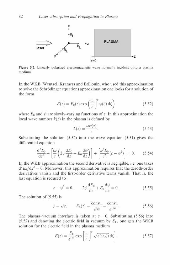
In the WKB (Wentzel, Kramers and Brillouin, who used this approximationto solve the Schrodinger equation) approximation one looks for a solution ofthe form

EðzÞ ¼ E0ðzÞ exp�i!

c

ðz ðÞ d

�ð5:52Þ

where E0 and are slowly-varying functions of z. In this approximation thelocal wave number kðzÞ in the plasma is defined by

kðzÞ ¼ ! ðzÞc

: ð5:53Þ

Substituting the solution (5.52) into the wave equation (5.51) gives thedifferential equation

d2E0

dz2þ�i!

c

�2

dE0

dzþ E0

d

dz

��þ�!2E0

c2ð"� 2Þ

�¼ 0: ð5:54Þ

In the WKB approximation the second derivative is negligible, i.e. one takesd2E0=dz

2 ¼ 0. Moreover, this approximation requires that the zeroth-orderderivatives vanish and the first-order derivative terms vanish. That is, thelast equation is reduced to

"� 2 ¼ 0; 2 dE0

dzþ E0

d

dz¼ 0: ð5:55Þ

The solution of (5.55) is

¼ffiffiffi"

p; E0ðzÞ ¼

const:ffiffiffiffi

p ¼ const:

"1=4: ð5:56Þ

The plasma–vacuum interface is taken at z ¼ 0. Substituting (5.56) into(5.52) and denoting the electric field in vacuum by EL, one gets the WKBsolution for the electric field in the plasma medium

EðzÞ ¼ EL

"1=4exp

�i!

c

ðz ffiffiffiffiffiffiffiffiffiffiffiffiffiffi"ð!; Þ

pd

�: ð5:57Þ

Figure 5.2. Linearly polarized electromagnetic wave normally incident onto a plasma

medium.


Thus, the amplitude of the electric field in the plasma is (using (5.40))

E0ðzÞ �EL

"1=4¼ EL

ð1� ðneðzÞ=necÞÞ1=4: ð5:58Þ

From the last equation it is evident that the amplitude increases at higherelectron density.

For the WKB approximation to be valid one requires that the secondderivative of the amplitude is much smaller than the first derivatives

d2E0

dz2� !E0

c

d

dz¼ E0

dkðzÞdz

;d2E0

dz2� !

c

dE0

dz¼ kðzÞ dE0ðzÞ

dz: ð5:59Þ

Adding the two equations of (5.59) and integrating, one obtains the followingnecessary condition for the WKB solution to be valid:

dE0

dz� kðzÞE0ðzÞ ¼

! E0

c: ð5:60Þ

Substituting (5.58) into (5.60), one gets the WKB approximation require-ment that the plasma density should vary slowly with the coordinate

dnedz

� 8�nec�ðzÞ

�1� neðzÞ

nec

�¼ 8�nec"ð!; zÞ

�ðzÞ : ð5:61Þ

We shall now solve the magnetic field in the WKB approximation. In thiscase the laser magnetic field is in the y direction, and therefore the waveequation for the magnetic field is given by the y component of equation(5.50). However, it is not necessary to solve this equation since the magneticfield is easily derived by using equation (5.38):

BðzÞ ¼ � ic

!

dEðzÞdz

¼�E0ðzÞ � ic

!

dE0ðzÞdz

�exp

�i!

c

ðzd

ffiffiffiffiffiffiffiffiffiffiffiffiffiffi"ð!; Þ

p �: ð5:62Þ

Using the WKB validity condition, as given by equation (5.60), one canneglect the second term in (5.62). Now using E0ðzÞ and ðzÞ from (5.56)and (5.58), we get the solution for the magnetic field in the plasma medium

BðzÞ ¼ EL"1=4 exp

�i!

c

ðzd

ffiffiffiffiffiffiffiffiffiffiffiffiffiffi"ð!; Þ

p �: ð5:63Þ

From equations (5.57), (5.58) and (5.63) one can see that while the electric fieldincreases at higher electron densities the magnetic field decreases accordingly.

The WKB approximation is not valid at the critical surface (where" ¼ 0, k ¼ 0 and � ¼ 1). In laser–plasma interaction the critical surfaceplays a very important role; part of the laser beam is absorbed there andthe other part is reflected from this surface. Therefore, the WKB solutionis mainly of pedagogical importance rather than of practical use. In thenext section we discuss an analytic solution (Ginzburg 1961) relevant alsoin the region of the critical density.

Slowly Varying Density—the WKB Approximation 83

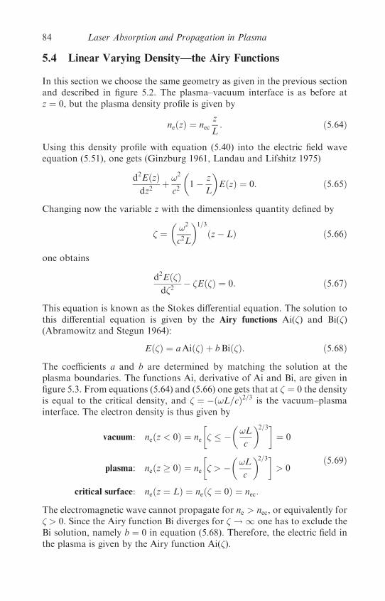
5.4 Linear Varying Density—the Airy Functions

In this section we choose the same geometry as given in the previous sectionand described in figure 5.2. The plasma–vacuum interface is as before atz ¼ 0, but the plasma density profile is given by

neðzÞ ¼ necz

L: ð5:64Þ

Using this density profile with equation (5.40) into the electric field waveequation (5.51), one gets (Ginzburg 1961, Landau and Lifshitz 1975)

d2EðzÞdz2

þ !2

c2

�1� z

L

�EðzÞ ¼ 0: ð5:65Þ

Changing now the variable z with the dimensionless quantity defined by

¼�!2

c2L

�1=3

ðz� LÞ ð5:66Þ

one obtains

d2EðÞd2

� EðÞ ¼ 0: ð5:67Þ

This equation is known as the Stokes differential equation. The solution tothis differential equation is given by the Airy functions Ai() and Bi()(Abramowitz and Stegun 1964):

EðÞ ¼ aAiðÞ þ bBiðÞ: ð5:68Þ

The coefficients a and b are determined by matching the solution at theplasma boundaries. The functions Ai, derivative of Ai and Bi, are given infigure 5.3. From equations (5.64) and (5.66) one gets that at ¼ 0 the densityis equal to the critical density, and ¼ �ð!L=cÞ2=3 is the vacuum–plasmainterface. The electron density is thus given by

vacuum: neðz < 0Þ ¼ ne

� �

�!L

c

�2=3�¼ 0

plasma: neðz � 0Þ ¼ ne

� > �

�!L

c

�2=3�> 0

critical surface: neðz ¼ LÞ ¼ neð ¼ 0Þ ¼ nec:

ð5:69Þ

The electromagnetic wave cannot propagate for ne > nec, or equivalently for > 0. Since the Airy function Bi diverges for ! 1 one has to exclude theBi solution, namely b ¼ 0 in equation (5.68). Therefore, the electric field inthe plasma is given by the Airy function Ai().


It is assumed that the dimension of the plasma L, from the vacuum tothe critical surface, is large in comparison with the electromagneticwavelength �L. On the other hand, L is of the order of the product of thelaser time duration �L and the expansion (towards the vacuum) plasma

Figure 5.3. The Airy functions Ai, its derivative and Bi.

Linear Varying Density—the Airy Functions 85

velocity uexp:

L � c

!¼ �L

2�; �LðpsÞ � 1:6

��Lmm

��107 cm=s

uexp

�: ð5:70Þ

From this relation one can see that the approximation of this section is notrelevant for the femtosecond lasers.

The plasma vacuum interface is at jj ¼ ð!L=cÞ2=3 � 1 (see (5.70));therefore, we can use the asymptotic expansion (Abramowitz and Stegun1964) of the Airy function Ai(z) for jj � 1:

Aið�Þ ¼ 1ffiffiffi�

p1=4

cos

�2

33=2 � �

4

�ð5:71Þ

in order to describe the electric field near the plasma–vacuum interface.Therefore, the electric field at z ¼ 0, from the plasma side, can beapproximated by the expression

Eðz ¼ 0; plasmaÞ ¼ affiffiffi�

p�

c

!L

�1=6cos

�2!c

3L� �

4

�

¼ a

2ffiffiffi�

p�

c

!L

�1=6

��exp

�i

�2!c

3L� �

4

��þ exp

��i

�2!c

3L� �

4

��: ð5:72Þ

Looking from the vacuum side, one has at z ¼ 0 the incident laser field EL

and a reflected wave given by EL expðiÞ:

Eðz ¼ 0; vacuumÞ ¼ EL½1þ expðiÞ�: ð5:73Þ

The requirement that the solution is continuous at the plasma–vacuuminterface (i.e. equating equations (5.72) and (5.73)) yields

a ¼ 2ffiffiffi�

p �!L

c

�1=6EL exp

�� i

�2!L

3c� �

4

��

¼ 4!L

3c� �

2¼ 4

3½�ðz ¼ 0Þ�3=2 � �

2:

ð5:74Þ

Substituting b ¼ 0 and a from (5.74) into (5.68), one gets the solution for theelectric field in the plasma:

EðÞ ¼ 2ffiffiffi�

p �!L

c

�1=6EL exp

�� i

�2!L

3c� �

4

��AiðÞ: ð5:75Þ

Ai() has a maximum at ¼ �1 (see figure 5.3); therefore, the ratio betweenthe maximum value of the electric field in the plasma and the laser electric


field in vacuum is ��Emax

EL

�� 1:90

�!L

c

�1=6: ð5:76Þ

For example, for a laser-produced plasma with a dimension L ¼ 100 mm anda laser wavelength of �L ¼ 1mm, one gets (using (5.70)) Emax=EL ffi 5:57.

The solution for the magnetic field is easily derived by using (5.38),

BðzÞ ¼ � ic

!

@EðzÞ@z

ð5:77Þ

the solution for E as given by (5.75), and the relation (5.66),

BðÞ ¼ �i2ffiffiffi�

p �c

!L

�1=6EL exp

�� i

�2!L

3c� �

4

��dAiðÞd

: ð5:78Þ

It is interesting to point out that when E is maximum, B is zero. At the criticalsurface, ¼ 0, one has (EL ¼ BL in Gaussian units)��Eðcritical surface)EL

�� ffi 1:26

�!L

c

�1=6��Bðcritical surface)EL

�� ffi 0:92

�!L

c

��1=6

:

ð5:79Þ

Note that the energy conservation (as expressed by the Poynting theorem, seeAppendix A) does not require the conservation of E� B.

So far we have discussed in this section the propagation of the electro-magnetic field without absorption. For absorption to occur, a damping ofenergy is required. This is possible only if the equations of wave propagationinclude collision processes, such as particle–particle and/or wave–particle.Taking into account electron–ion collisions, the dielectric function is

" ¼ 1�!2pe

!ð!þ i�eiÞ¼ 1� z

L½1þ ið�ei=!Þ�ð5:80Þ

where a linear density profile is assumed for the second equality in thisequation. For a wave propagating in the z direction with an electric field inthe x direction, EðzÞ, one has to solve the wave equation (5.51) with thedielectric function of (5.80). Assuming in this equation that the electron–ion collision frequency is a constant equal to its value at the critical surface,i.e. �ei ¼ �eiðnecÞ ¼ �c, equation (5.51) then takes the form

d2EðzÞdz2

þ !2

c2

�1� z

L½1þ ð�c=!Þ�

�EðzÞ ¼ 0: ð5:81Þ

Change of variables

¼�

!2

c2L½1þ ið�c=!Þ�

�1=3�z� L

�1þ i

�c!

��ð5:82Þ

Linear Varying Density—the Airy Functions 87

yields the Stokes equation (5.67) for a complex variable. Note that for �c ¼ 0the change of variables is identical to that of equation (5.66). The solution tothe differential equation is, as before, Eð; plasmaÞ ¼ aEiðÞ and

Eðz ¼ 0; vacuumÞ ¼ EL½1þ expðiÞ� ¼ Ein þ Eout

¼ 4

3

�!L

c

�1þ i

�c!

��

2� R þ iI

ð5:83Þ

where Ein ¼ EL is the incoming electric field and Eout is the outgoing electricfield from the plasma. Since is complex we not only get a phase shift (asbefore, in (5.74)), but also a damping of the wave determined by the imaginaryvalue of (I ¼ 4�cL=3c). The absorbed fraction fa of the input laser energy is

fa ¼jEinj2 � jEoutj2

jEinj2¼ E2

L � E2L expð�2IÞE2L

: ð5:84Þ

Using the value of I, one gets the absorption coefficient

fa ¼ 1� exp

�� 8�cL

3c

�: ð5:85Þ

In comparing this result with the one obtained in (5.25) (both cases with thesame density profile), one can see that the absolute value of the coefficient inthe exponent of equation (5.85) is larger than the one in (5.25) by a factor of5/4, implying a larger absorption coefficient. This can be understood since inthat deriving the last equation we assumed a constant collision frequencylarger than or equal to the real collision frequency. The larger the collisionfrequency the larger is the absorption coefficient.

5.5 Obliquely Incident Linearly Polarized Laser

Without any loss of generality we choose the coordinates in such a way thatthe laser propagates in the y–z plane, i.e. the wave vector k is in this plane.The vacuum–plasma interface is chosen at z ¼ 0 and the electromagneticwave is obliquely incident at an angle �0 to the normality of this surface.

The electron density neðzÞ is assumed to be linear as in the previoussection. � is the angle between the electron density gradient and the wavevector k. The electric field is in the x direction for s-polarization and in they–z plane for the p-polarization (see figure 5.4). Therefore, the componentsof the electromagnetic fields are

the wave vector: k ¼ ½0; ky ¼ ð!=cÞ sin �; kz ¼ ð!=cÞ cos ��

s-polarization: E ¼ ½Exðy; zÞ; 0; 0�;B ¼ ½0;Byðy; zÞBzðy; zÞ�

p-polarization: E ¼ ½0;Eyðy; zÞ;Ezðy; zÞ�;B ¼ ½Bxðy; zÞ; 0; 0�:

ð5:86Þ


The dispersion relation (5.46) is

!2 ¼ !2pe þ ðk2y þ k2zÞc2: ð5:87Þ

Sincewe have only a z-dependence in the electron density, one has a constant ky:

ky ¼!

csin �0 ð5:88Þ

while kz is a function of z. The relation (5.88) can be seen as the photonmomentum (¼ hk, h is Planck’s constant) conservation in the y direction.

The reflection of the laser occurs at the surface where kz ¼ 0, i.e. where� ¼ 908. Using the linear density relation (5.64) and equations (5.40), (5.87)and (5.88), one gets

neðkz ¼ 0Þ ¼ nec cos2 �0; nec ¼

me!2

4�e2

!peðkz ¼ 0Þ ¼ ! cos �0

zðkz ¼ 0Þ ¼ L cos2 �0

"ðkz ¼ 0Þ ¼ sin2 �0:

ð5:89Þ

Solving the wave equations for the electromagnetic fields, one finds that thereis no sharp cut-off as might appear from the geometrical optics (figure 5.4),but an exponential decay of the field amplitudes for z > L cos2 �0.

Figure 5.4. A linearly polarized laser propagating in the y–z plane.

Obliquely Incident Linearly Polarized Laser 89

5.5.1 s-polarization

In this case the electric field is in the x direction and the wave equation for thex-component of the electric field, ExðzÞ, is

@2Ex

@y2þ @2Ex

@z2þ !2"ðzÞ

c2Ex ¼ 0: ð5:90Þ

The electric field is a function of z and the phase exp½iðkyyþ kzzÞ�. Since kzz isa function of z it can be included in the amplitude and using (5.88) the electricfield can be written in the form

Ex ¼ EðzÞ exp�i!y sin �0

c

�: ð5:91Þ

Substituting (5.91) into (5.90) and using " ¼ 1� z=L yields

d2EðzÞdz2

þ !2

c2

�1� z

L� sin2 �0

�EðzÞ ¼ 0: ð5:92Þ

Changing the variable z to defined by

¼�!2

c2L

�1=3ðz� L cos2 �0Þ ð5:93Þ

one gets the Stokes differential equation (5.67) with the solution (5.75).We shall now calculate the absorption of the s-polarized laser with

oblique incidence. The dielectric function given in equation (5.80) is taken,but unlike in the previous section the electron–ion collision frequency isnot a constant. For the linear electron density profile the electron–ioncollision frequency is

�ei ¼ �cnenec

¼ �cz

L: ð5:94Þ

The dispersion relation (5.87) can be written as

k2z ¼!2

c2½"ðzÞ � sin2 �0�: ð5:95Þ

Using (5.80) and (5.94), one gets

kz ¼!

c

�cos2 �0 �

z

L½1þ ið�cz=!LÞ�

�1=2� kR þ ikI: ð5:96Þ

We shall assume that �ei=!� 1 and use the WKB approximation to calcu-late the absorption coefficient defined by (5.84). Using equation (5.57), where

ffiffiffi"

p¼ ckz

!ð5:97Þ


one gets

jEðzÞj2 / exp

��2

ðzkIðÞ d

�: ð5:98Þ

Expanding (5.96) for �c=!� 1, and taking the integral in (5.98) twice from 0to L cos2 �0 (the ‘turning’ surface where the laser is reflected), i.e. from theplasma–vacuum boundary to the ‘turning’ surface and back to theplasma–vacuum boundary, one gets

jEoutðz ¼ 0Þj2

jEinðz ¼ 0Þj2¼ exp

4!

cIm

ðL cos2 �0

0d

��cos2 �0 �

L

�þ i

�c!

2

L2

�1=2( )ð5:99Þ

where Im stands for the imaginary part. Doing the integral and taking theimaginary part, one gets for the absorption coefficient

fa ¼ 1� jEoutj2

jEinj2¼ 1� exp

�� 32�cL cos5 �0

15c

�: ð5:100Þ

This result for �0 ¼ 0 is identical to the one obtained in equation (5.25) forthe same electron density profile. Equation (5.100) is frequently used in theliterature in order to understand the experimental results for the inversebremsstrahlung absorption in laser–plasma interactions.

5.6 p-Polarization: the Resonance Absorption

Laser light might be absorbed by resonance absorption in the plasma. Thesolution of Maxwell’s equations show (Denisov 1957, Ginsburg 1961,Friedberg et al. 1972, Speziale and Catto 1977) that p-polarized light incidenton a steeply rising plasma density at an angle different from zero fromnormal incidence has a singularity in the magnitude of the oscillating electricfield in the plasma. This electric field resonantly drives an electron plasmawave (see next chapter). The damping of this wave is possible either by colli-sion or collisionless processes, so that resonance absorption is effective evenwhen the electron–ion collision frequency, �ei, is very small. The resonanceabsorption is larger than the inverse bremsstrahlung for the followingvariables: high plasma temperatures, i.e. high laser intensities; longer laserwavelength, i.e. lower values of nc; and short plasma scale length, L. Forhigh laser intensities, e.g. IL�

2L > 1015 (W/cm2) mm2, at the right laser polar-

ization (p-polarization) and angle of incidence, up to about 50% absorptionmay occur by resonance absorption. The main feature of the resonantabsorption is the creation of hot electrons, since only a minority of theplasma electrons acquires most of the absorbed energy in contrast to collisionabsorption (inverse bremsstrahlung), which heats all of the electrons.

p-Polarization: the Resonance Absorption 91

For the p-polarization obliquely incident laser it is convenient to solve theequation for the magnetic field, which is in the x direction. Similar to thearguments leading to equation (5.91), the magnetic field can be presented by

Bx ¼ BðzÞ exp�i!y sin �0

c

�: ð5:101Þ

Substituting (5.101) into the wave equation (5.50) for the magnetic field, onehas to solve the differential equation

d2BðzÞdz2

� 1

"

d"

dz

dBðzÞdz

þ !2

c2ð"� sin2 �0ÞBðzÞ ¼ 0: ð5:102Þ

Using " from (5.80) for �ei ¼ 0, equation (5.102) can be rewritten as

d2BðzÞdz2

þ 1

ðz� LÞdBðzÞdz

��!2

Lc2

�½ðz� LÞ þ L sin2 �0�BðzÞ ¼ 0: ð5:103Þ

Substituting

¼�!2

Lc2

�1=3ðz� LÞ; � ¼

�!L

c

�1=3sin �0 ¼

�2�L

�L

�1=3sin �0 ð5:104Þ

equation (5.103) takes the form

d2B

d2� 1

dB

d� ð þ �2Þ ¼ 0: ð5:105Þ

Note that � and are dimensionless. The differential equation (5.105)depends on a single parameter � . This equation is singular at ¼ 0, i.e. atthe critical surface. Near the critical surface, where � �2, one has theequation

d2B

d2� 1

dB

d� �2 ¼ 0: ð5:106Þ

The solution of this differential equation is (one can easily check the solutionby direct substitution into (5.106))

BðÞ ¼ B0ð1þ 12 �

22 ln Þ ð5:107Þ

where B0 is a constant. The magnetic field Bxðy; zÞ is thus given near thecritical surface from (5.101), (5.104) and (5.107):

Bxðz ! L; yÞ ¼ B0 1þ �2

2

�!2

Lc2

�2=3ðz� LÞ2

�1

3ln

�!2

Lc2

�þ lnðz� LÞ

�( )

� exp

�i!y sin �0

c

�: ð5:108Þ


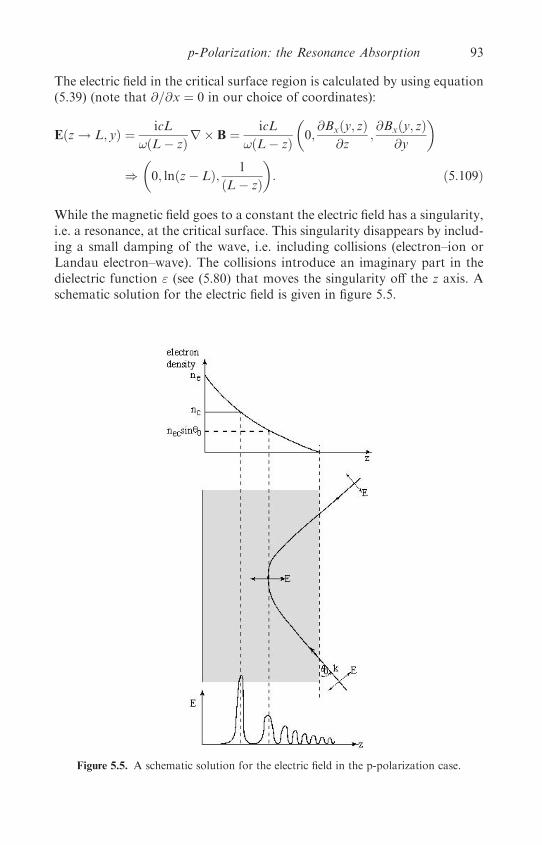
The electric field in the critical surface region is calculated by using equation(5.39) (note that @=@x ¼ 0 in our choice of coordinates):

Eðz ! L; yÞ ¼ icL

!ðL� zÞr � B ¼ icL

!ðL� zÞ

�0;@Bxðy; zÞ

@z;@Bxðy; zÞ

@y

�

)�0; lnðz� LÞ; 1

ðL� zÞ

�: ð5:109Þ

While the magnetic field goes to a constant the electric field has a singularity,i.e. a resonance, at the critical surface. This singularity disappears by includ-ing a small damping of the wave, i.e. including collisions (electron–ion orLandau electron–wave). The collisions introduce an imaginary part in thedielectric function " (see (5.80) that moves the singularity off the z axis. Aschematic solution for the electric field is given in figure 5.5.

Figure 5.5. A schematic solution for the electric field in the p-polarization case.


The existence of the singularity in the electric field at the critical surfacecan be recognized immediately by considering the followingMaxwell equationin the dielectric plasma medium:

0 ¼ r � ð"EÞ ¼ "r � Eþ ðr"Þ � E: ð5:110Þ

Therefore, for " ¼ "ðzÞ one has

r � E ¼ � 1

"

@"

@zEz: ð5:111Þ

The resonance is only for the p-polarization where the electric field in the zdirection does not vanish, but the dielectric function can vanish there(" ¼ 0 at ! ¼ !pe). When the p-polarized laser is reflected (when � ¼ 908)the electric field has a component parallel to the density gradient. Thisfield causes charge separation as the electron oscillates along the gradient.The electron density wave variations (�n) due to this effect are given by

�n � r � E ¼ � 1

"

@"

@zEz ð5:112Þ

where r � E from (5.111) was substituted into (5.112). One can see that for aplasma frequency equal to the laser frequency (where " vanishes) one has aresonance in the plasma wave. Therefore, the electron plasma wave is excitedresonantly at the critical density for the p-polarized laser radiation.

Let us check the consistency of this analysis with the solution of theelectric field near the critical surface (equation (5.109)). From this equationone gets

Eðz ! LÞ � 1

ðz� LÞ

�ne � r � Eðz ! LÞ � 1

ðz� LÞ2� Eðz ! LÞ"ðz ! LÞ

ð5:113Þ

as predicted in the above picture by equation (5.111). Therefore, the chargeseparation near the critical surface oscillates with the plasma frequency andexcites the plasma wave resonantly.

No laser absorption is possible without damping. The dissipation of thelaser energy is possible by electron–ion or electron–wave collisions, or anyother mechanism that makes the dielectric function complex. The absorbedenergy flux Iabs [dimension of energy/(area time)] can also be presented as

Iabs ¼ð�eff

�E2

8�

�dz ð5:114Þ

where �eff is the effective collision frequency and the integral is along theelectromagnetic ray path. The fraction fa of the absorbed energy is therefore


given by

fa ¼IabsIL

¼

ð�effE

2 dz

cE2L

: ð5:115Þ

For the linear density profile and a p-polarized laser it has been calculated(Ginzburg 1961, Pert 1978) that the laser absorption is

fa ffi 36�2½Aið�Þ�3

jdAið�Þ=dð�Þj ð5:116Þ

where Ai is the Airy function and � is defined in equation (5.104). fa vanishesat t ¼ 0, goes to zero for � � 2, and has a maximum value at about � � 0.8with a maximum absorption of about 50%, i.e.

fað� � 0:8Þ ffi 0:5: ð5:117Þ

It has been shown (Forslund et al. 1975) that for ions at rest the absorption ispractically unchanged up to electron temperatures of 100 keV.

Substituting for � ¼ 0.8 in equation (5.104) yields sin �0 ¼ 0:42�L=L.For a plasma dimension L � �L, the resonant absorption is confined toa light incident almost perpendicular (�0 � 08). However, for large laserirradiances IL > 1016 W/cm2, the ponderomotive force steepens the plasmadensity and in this case L � �L is possible. Also for small laser pulse dura-tion, �L < 20 ps, the plasma dimension is smaller than the laser wavelengthin vacuum. These small plasma dimensions have peak resonance absorptionat about 258 (see figure 5.6). The high electric field near the critical surface inthese cases can accelerate electrons to energies much higher than the plasmatemperature.

Figure 5.6. Schematic absorption fraction for a p-polarized laser in comparison with an

s-polarized laser for a given laser intensity.


5.7 Femtosecond Laser Pulses

For this class of lasers the solid target is heated faster than the time scale forhydrodynamic expansion. The plasma medium in this case has a densityequal to its initial solid density during the laser pulse duration. The typicallaser pulse duration is of the order of �L 100 fs. During this time thelaser is absorbed and heats the target along a skin depth � � 200 A, avalue much larger than the surface expansion 10 A. For a laser spotmuch larger than the skin depth one can assume a one-dimensional problem.

We assume that the laser is radiated in the z direction and is normallyincident on a solid target (positioned in the x–y plane) at z ¼ 0. The waveequation of the electric field for a linearly polarized monochromatic waveat normal incidence is (see (5.51))

@2EðzÞ@z2

þ "ð!; zÞ!2EðzÞc2

¼ 0: ð5:118Þ

This equation is also known as the Helmholtz equation (Milchberg and Free-man 1989). "ð!; zÞ is the dielectric permittivity of the target related to theelectrical conductivity �E by (see section 2.7)

" ¼ 1þ i4��E!

: ð5:119Þ

For a constant " and a vanishing electric field at infinity, the solution ofequation (5.118) is

EðzÞ ¼ Eð0Þ exp�� z

�

�ð5:120Þ

where EðzÞ is the electric field transmitted into the solid target. Denoting byEi and Er the incident and reflected electric field accordingly, one can write

Ei ¼ Eð0Þ exp½iðkz� !tÞ�; Er ¼ffiffiffiffiR

pEð0Þ exp½ið�kz� !tÞ� ð5:121Þ

where R is the reflection coefficient. The absorption coefficient A is given by(Landau and Lifshitz 1975, Born and Wolf 1980)

A ¼ 1� R; R ¼�� 1�

ffiffiffi"

p

1þ ffiffiffi"

p��2

¼ ðnR � 1Þ2 þ n2I

ðnR þ 1Þ2 þ n2Ið5:122Þ

where the complex index of refraction is defined asffiffiffi"

p¼ nR þ inI: ð5:123Þ

Substituting the solution (5.120) into (5.118) yields the skin depth �:

� ¼ iffiffiffi"

p c

!: ð5:124Þ


Substituting for the dielectric function (see section 2.7),

" ¼ 1�!2pe

!ð!þ i�Þ ð5:125Þ

where !pe is the plasma frequency and � is the electron effective collisionfrequency (e.g. � ¼ �ei), one gets (More et al. 1988)

� ¼ c

!pe

�1þ ið�=!Þ

1� ð!2=!2peÞ � ið�!=!2

peÞ

�1=2

� c

!pe

�1þ i

�

!

�1=2for !pe � !: ð5:126Þ

In our plasma medium (solid target) !pe � ! and therefore the last approx-imation is justified. The skin depth is therefore given by

� ¼

c

!pe

for�

!� 1 and

!

!pe

� 1

c

!pe

��

2!

�1=2for

�

!� 1 and

!

!pe

� 1:

8>>><>>>:

ð5:127Þ

For the last stage the following algebraic relation was used:

ffiffiffiffiffiffiffiffiffiffiffiffiaþ ib

p¼ 1ffiffiffi

2p ða2 þ b2Þ1=4

��1þ affiffiffiffiffiffiffiffiffiffiffiffiffiffiffi

a2 þ b2p

�1=2þ i

�1� affiffiffiffiffiffiffiffiffiffiffiffiffiffiffi

a2 þ b2p

�1=2" #: ð5:128Þ

Using the dielectric function from (5.125) into the absorption coefficient A in(5.122), one gets

A ¼

2�

!pe

for�

!� 1 and

!

!pe

� 1

2�

!pe

ffiffiffi!

�

rfor

�

!� 1 and

!

!pe

� 1:

8>>><>>>:

ð5:129Þ

For the above analysis it was assumed that the dielectric function " is a constantin space and time.However, in general this is a very crude approximation, sinceduring the (time-dependent) laser pulse duration, the dielectric function " is notconstant due to the change of electron and ion temperatures as well as possiblechange of the electron number density. The electron collision frequency � andthe electrical conductivity �E are functions ofTe,Ti and ne, which are functionsof space and time. In this case the following approach is more suitable.

The Joule heating gives the laser power deposition into the target perunit volume:

Qðz; tÞ ¼ 12Ref�Eðz; tÞgjEj2: ð5:130Þ

Femtosecond Laser Pulses 97

Note that �Eð!; zÞ and "ð!; zÞ vary with time t on a time scale much longerthan 2�=!. Both �E and " depend on z and t through Teðz; tÞ and Tiðz; tÞ,while Q and EðzÞ also depend on t via the laser pulse temporal intensityprofile, ILðtÞ. A good approximation for the intensity profile is

IL � I0 sin2

��t

2�L

�for 0 t 2�L

IL � 0 for t 0; t � 2�L

ð5:131Þ

where �L is the FWHMpulse duration. The absorption coefficientAmeasuredat a given location ðx; yÞ on the target surface ðz ¼ 0Þ is averaged over thetemporal pulse profile:

A ¼

ð2�L0

dt

ð10Qðz; tÞ dz

ð2�L0

ILðtÞ dt: ð5:132Þ

In order to calculate the absorption coefficient A in (5.132) one has to use theheat deposition Qðz; tÞ given in (5.130), which requires knowledge of theelectric field E and electric conductivity �E inside the target.

Since the interaction of the femtosecond laser has a solid state ofmatter during the laser pulse duration, a knowledge of quantum solid state

physics is required (Ziman 1960, Ashcroft and Mermin 1976, Gantmakherand Levinson 1987, Peierls 2001). In the following we shall outline theingredients and some approximated formulas for the calculation of theabsorption of femtosecond lasers by solid targets. The dielectric permittivity", or equivalently the electrical conductivity �E (equation (5.119)), containsthe contribution from both the inter-band and intra-band absorptionmechanism:

�E ¼ �bb þ �D: ð5:133Þ

The subscript bb and D stand for inter-band (band–band transition) absorp-tion and intra-band absorption, known as the Drude contribution (theinverse bremsstrahlung absorption) given by

�D ¼ nee2

meff

�� þ i!

�2 þ !2

�: ð5:134Þ

Regarding the band–band transitions there are two distinct possibilities. Onetransition can occur between the Bloch-electron bands (between the lower(e.g. first band) and the upper (e.g. second band) one-electron bands in thefirst Brillouin zone), as in aluminium metal (Ashcroft and Sturm 1971).The other possibility is the transition between the occupied atomic statesand the Fermi surface. The bb transitions will not be further discussed


here, although they can contribute significantly to the absorption of femto-second lasers (Fisher et al. 2001).

The electric conductivity in equation (5.134) is a function of the electroncollision frequency �, which in our case is the total momentum relaxationrate for electrons in the solid. This collision frequency has two contributions,

� ¼ �e-phðTe;TiÞ þ �e-eðTeÞ ð5:135Þ

where �e-ph and �e-e are the electron momentum relaxation rates due toelectron–phonon and electron–electron collisions, respectively. Since � is afunction of Te and Ti it is necessary to solve the energy equations (as givenin section 3.3):

CeðTeÞ@Te

@t¼ @

@z

��ðTeÞ

@Te

@z

��UðTe;TiÞ þQðz; tÞ

CiðTiÞ@Ti

@t¼ UðTe;TiÞ

ð5:136Þ

where Ce and Ci are the electron and ion heat capacities at constant volume(dimension [erg/(cm3 K)]), � is the electron heat conductivity (dimension[erg/(cm s)]) and U is the energy transfer rate from electrons to ions andcan also be written by

U ¼ ðTe � TiÞ: ð5:137Þ

To calculate �,U and �E as functions of Te and Ti, knowledge of the phononspectrum (i.e. the dispersion relation) and the electron–phonon interactionmatrix element is required (Kaganov et al. 1957).

The phonon spectrum !phðqÞ for longitudinal phonons, where q is thephonon wave vector, can be approximated by (Dederichs et al. 1981)

!phðqÞ ¼ qs for q qb

!phðqÞ ¼ qbs for q � qbð5:138Þ

where s is the longitudinal sound velocity (e.g. s ¼ 6:4� 105 cm/s foraluminium) and qb is a parameter determined by fitting the d.c. electricalconductivity data.

Since electron–phonon scattering in metals occurs primarily via a singlelongitudinal phonon absorption or emission (by an electron), the followingmatrix element squared is assumed (Gantmakher and Levinson 1987):

jMðk ! k0 qÞj2 ¼

�hw20q

2V�s�k0�k;�q for q qb

�hw20qb

2V�s�k0�k;�q for q � qb

8>>><>>>:

ð5:139Þ


where w0 is the deformation potential constant, � and V are the mediumdensity and volume and �hq is the quasi-momentum of the absorbed (oremitted) phonon as the electron wave vector has changed from k to k

0.The � in (5.139) takes care of the momentum conservation in these processes.The transition probability is given by

Wðk ! k0 qÞ ¼ 2�

�hjMðk ! k

0 qÞj2ðNq þ 12 1

2Þ�ðEk � Ek0 � �h!phðqÞÞ

ð5:140Þ

where Ek ¼ EF þ �h2fkFðjkj � jkFjÞ=2meffg and the � describes the energyconservation. Nq is the population of longitudinal phonon mode in thefirst Brillouin zone with the reduced momentum qred ¼ q� K, where K is acorresponding vector of the reciprocal lattice. q may lie outside the firstBrillouin zone (Umklapp process) but qb is inside the first Brillouin zone.Nq is the Bose–Einstein distribution function given by

Nq ¼�exp

��h!phðqredÞ

kBTi

�� 1

��1

: ð5:141Þ

The rate of electron–phonon (i.e. electron–ion) energy exchange U iscalculated by the method described by Kaganov et al. (Kaganov et al. 1957,Allen 1987, Fisher et al. 2001):

U ¼ 1

ð2�Þ3ð �

dNq

dt

��h!q4�q

2 dq: ð5:142Þ

Using the phonon dispersion relation (5.138) and the matrix element (5.139),we get equation (5.143). Note that UðTe ¼ TiÞ ¼ 0 as required from physicalconsideration. For aluminium with ion temperatures larger than 300K equa-tion (5.143) yields a value in the domain (3.7–3.9)� 1018 erg/(cm3 sK). Thisvalue is in very good agreement with Wang and Downer (Wang and Downer1992) and is by a factor of 1.5–3 larger than the empirical values of Eidmanet al. (Eidman et al. 2000):

U ¼ ðTe � TiÞ

¼ sw20m

2eff

4�3�h2�

�

��hs

kBTe

��5 ðð�hqbs=kBTeÞ

0

x4 dx

ex � 1��

�hs

kBTi

��5 ðð�hqbs=kBTiÞ

0

x4 dx

ex � 1

þ q3b2ð4k2F � q2bÞ

��exp

��hqbs

kBTe

�� 1

��1

��exp

��hqbs

kBTi

�� 1

��1�

8>>>><>>>>:

9>>>>=>>>>;:

ð5:143Þ


The electron heat conductivity is given by

�ðTe;TiÞ �Ce

3�

�v2F þ 3kBTe

me

�ð5:144Þ

where vF ¼ �hkF=meff is the Fermi velocity, meff is the effective mass of theelectron in the solid and �h ¼ 2�h, where h is the Planck constant. TheFermi momentum kF is related to the Fermi energy EF ¼ ð�hkFÞ2=2me,where me is the (free) electron mass. � is given by (5.135) and it has twocontributions, one from the electron–electron collisions and the secondfrom the electron–phonon collisions defined by

�e-ph ¼Xk0

Wðk ! k0 qÞ

�ðk� k

0Þ � kk2

��1� f ðk0;TeÞ1� f ðk;TeÞ

�: ð5:145Þ

f ðk;TeÞ, the Fermi–Dirac distribution, describes the electron population

f ðk;TeÞ ¼�exp

�Ek � �ðTeÞ

kBTe

�þ 1

��1

ð5:146Þ

where � is the free electron chemical potential. One can see from (5.145) that� is the electron momentum relaxation rate due to collisions with phonons.For temperatures higher than the Fermi temperature the �e-ph has to bechanged to the plasma frequency collisions �ei (see section 2.2).

We do not give here a detailed calculation of �e-ph, but point out thatfor temperature lower than the Fermi temperature the electron–phonon colli-sion frequency is independent of Te and the following approximation is valid:

�e-ph � B1T i for Ti TF ¼ EF

kBð5:147Þ

where B1 is a constant. If solid–liquid phase transition takes place then theapproximation (5.147) is valid for Te ¼ Ti < Tm (Tm is the melting tempera-ture) and for TF > Te ¼ Ti > Tm, and �e-ph is expected to have a jump at Tm.However, on the femtosecond time scale Te is not equal to Ti and it isconceivable that the solid–liquid transition time is longer than the laserpulse duration, so that in this case equation (5.147) might be a good approx-imation. For Te > TF this dependence on Ti is no longer satisfied. However,in this domain �e-ph is significantly smaller than the momentum relaxationrate in electron–electron collisions �e-e, given by

�e-e �

EF

�h

�Te

TF

�2� B2T

2e for Te < TF

EF

�h

�Te

TF

��3=2

for Te > TF:

8>>>><>>>>:

ð5:148Þ

In the second approximation of (5.148) the logarithmic factor in Te wasignored. The values of w0 and qb in the above equations are determined by


fitting the d.c. electrical conductivity with the experimental data (Zinovev1996) as a function of temperature. Using (5.134), (5.147) and (5.148), onehas to fit the following expression in order to obtain the values of w0 and qb:

�Eðd:c:Þ � �Eð! ¼ 0Þ ¼ nee2

meff�

�ðT e ¼ Ti ¼ T < TmÞ ¼ B1T þ B2T2:

ð5:149Þ

For example, for aluminium with an electron effective mass meff ¼ 1:20me

one gets w0 ¼ 5.16 eV and qb ¼ 4:77� 107 cm�1. Figure 5.7 shows thecalculated values of the collision frequency �ðTe;TiÞ as a function of theelectron temperature for several values of ion temperatures.

In order to solve the energy equations (5.136) one has to know also theelectron and ion heat capacities at constant volume Ce and Ci. Ce can beapproximated by

CeðlowÞ ¼�2nek

2BTe

2EF

for kBTe � EF

CeðhighÞ ¼ 1:5kBne for kBTe � EF

Ce ¼CeðlowÞCeðhighÞffiffiffiffiffiffiffiffiffiffiffiffiffiffiffiffiffiffiffiffiffiffiffiffiffiffiffiffiffiffiffiffiffiffiffiffiffiffiffiffiffiffiffiffi

CeðlowÞ2 þ CeðhighÞ2q for kBTe � EF:

ð5:150Þ

Figure 5.7. Calculated collision frequency �ðTe;TiÞ for several values of ion temperature Ti.


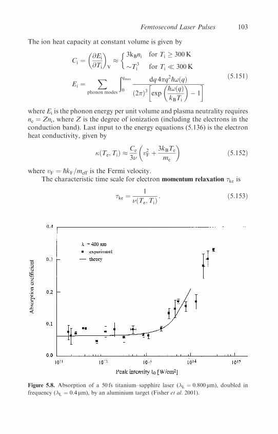
The ion heat capacity at constant volume is given by

Ci ¼�@Ei

@Ti

�V

��3kBni for Ti � 300K

T3i for Ti � 300K

Ei ¼X

phonon modes

ðqmax

0

dq 4�q2�h!ðqÞ

ð2�Þ3�exp

��h!ðqÞkBTi

�� 1

� ð5:151Þ

where Ei is the phonon energy per unit volume and plasma neutrality requiresne ¼ Zni, where Z is the degree of ionization (including the electrons in theconduction band). Last input to the energy equations (5.136) is the electronheat conductivity, given by

�ðTe;TiÞ �Ce

3�

�v2F þ 3kBTe

me

�ð5:152Þ

where vF ¼ �hkF=meff is the Fermi velocity.The characteristic time scale for electron momentum relaxation �ke is

�ke ¼1

�ðTe;TiÞ: ð5:153Þ

Figure 5.8. Absorption of a 50 fs titanium–sapphire laser (�L ¼ 0:800 mm), doubled in

frequency (�L ¼ 0:4 mm), by an aluminium target (Fisher et al. 2001).


For aluminium at room temperature this characteristic time scale is domi-nated by electron–phonon collisions and equals �k ¼ 8 fs, while at theFermi temperature (TF ¼ 0:135� 106 K) the electron–electron collisionsdominate and �k ¼ 0:1 fs.

The characteristic times of electron energy relaxation (cooling) �Ee, andion (i.e. lattice) energy relaxation (heating) �Ei, are defined by

�Ee ¼CeðTe � TiÞ

U¼ Ce

; �Ei ¼

Ci

: ð5:154Þ

For aluminium the electron energy relaxation time increases from�EeðTe ¼ 300KÞ � 100 fs to �EeðTe ¼ TFÞ � 10 ps mainly due to the increasein Ce(Te), while �EiðTe > 300KÞ � 6 ps since both Ci and are nearlyconstant in Te and Ti at room temperature and above.

We end this chapter with figure 5.8, showing the detailed results of theabove calculations for a titanium–sapphire laser (�L ¼ 50 fs, �L ¼ 0:800 mm)interacting with an aluminium target. The experimental data for a doubledfrequency (�L ¼ 0:4 mm) indicate the domain where the above approximationsare relevant.


Chapter 6

Waves in Laser-Produced Plasma

6.1 Foreword to Parametric Instabilities

The dispersion relation for electron plasma waves is developed in section 2.6.Some changes in the dispersion relation of electron and ion waves due toponderomotive force are given in section 4.3. In this chapter we discussmainly the parametric instabilities in laser–plasma interactions.

All material substances, including plasma, interact nonlinearly withhigh-power lasers leading to parametric instabilities. A parametric instability

is defined in general by the nonlinear phenomenon where a periodic variationin the medium induces growing oscillations at a different frequency. In solids,liquids and gases these instabilities arise due to the nonlinear polarizability ofthe material. In a plasma medium the nonlinear effects are caused by suchterms as v� B, v �rv, r � ðnvÞ, ponderomotive forces, changes of mass dueto relativistic velocities, velocity-dependent collision frequency, etc. Theseterms can cause a large amplitude wave, called the pump wave, whichprovides the driving force to excite other wave modes in the plasma.

In the absence of a pump wave and a magnetic field, three modes ofpropagation are possible in plasma:

(a) electromagnetic wave;(b) electron wave, known as plasmon or Langmuir wave (sometimes denoted

by ‘high frequency electrostatic plasma wave’); and(c) ion wave, also called acoustic wave (sometimes denoted by ‘low frequency

electrostatic ion-acoustic wave’).

Neglecting the ponderomotive forces, the dispersion relations of these wavesare

electromagnetic wave: !2 ¼ !2pe þ c2k2 ð6:1Þ

electron wave ¼ plasmon: !2 ¼ !2pe þ 3k2v2e ð6:2Þ

105

ion wave ¼ acoustic wave: ! ¼ kcs ¼ k

�ZkBTe

mi

�1=2ð6:3Þ

where ! and k are the wave frequency and wave number respectively and!pe ¼ ð4�e2ne=meÞ1=2 is the electron plasma frequency. me and mi are theelectron and ion mass respectively, Z is the degree of ionization, c is thespeed of light and cs is the sound velocity, Te, ve and ne are the electrontemperature, velocity and density respectively, and kB is the Boltzmannconstant. Te much larger than the ion temperature is assumed. Equations(6.1) and (6.2) were derived in sections 2.7 and 2.6 respectively, whileequation (6.3) is developed in section 6.6 of this chapter (the soliton section).

A high-power laser wave (denoted by the incoming ‘photon’), serving asa pump, can induce the following parametric instabilities in plasma:

Wave�wave interaction

photon ! photonþ acoustic ðstimulated Brillouin scattering ¼ SBSÞ

photon ! photonþ plasmon ðstimulated Raman scattering ¼ SRSÞ

photon ! acousticþ plasmon ðdecay instabilityÞ

photon ! plasmonþ plasmon ðtwo-plasmon instabilityÞ

Wave�particle interaction

photonþ particle ! photonþ particle ðstimulated Compton scatteringÞ

photonþ particle ! plasmonþ particle ðstimulated Compton scatteringÞ

photonþ particle ! acousticþ particle ðstimulated Compton scatteringÞð6:4Þ

In (6.4) ‘photon’, ‘acoustic’ and ‘plasmon’ mean electromagnetic, ion andelectron waves respectively. The energy and momentum conservation in thewave–wave interaction is described by

!0 ¼ !1 þ !2; k0 ¼ k1 þ k2 ð6:5Þ

where !0 and k0 are the frequency and wave number of the pumping laserfield that decays into two waves (!1, k1) and (!2, k2). Using these conserva-tion laws and the dispersion relations (6.1), (6.2) and (6.3), the wave–waveinteractions are induced in the following domain:

1. A laser pump with frequency near the plasma frequency, !0 � !pe, maydecay into a plasmon and an ion wave, resulting in absorption of thelaser. This effect happens near the critical surface since !0 � !pe impliesne � nec, where nec is the critical density.

2. A laser pump with frequency !0 > 2!pe may decay into a photon and aplasmon (SRS), leading to laser scattering, including backscattering.

106 Waves in Laser-Produced Plasma

This instability reduces the laser absorption. !0 > 2!pe implies that thisinstability occurs at ne <

14 nec.

3. A laser pump with frequency !0 > !pe may decay into a photon and anacoustic wave (SBS), resulting in backscattering and thus reduced laser

Figure 6.1—continues.

Foreword to Parametric Instabilities 107

absorption. SBS contains a low-energy ion wave that takes only a smallfraction of the laser energy, while the rest of the energy can be scatteredout of the plasma. !0 > !pe implies that this instability occurs at ne < nec.

4. A laser pump with frequency !0 ¼ 2!pe may decay into two plasmons,inducing laser absorption. This phenomenon happens at an electrondensity ne ¼ 1

4 nec.

A schematic description of the conservation laws given in equations (6.5) aregiven in figure 6.1 (Hughes 1980), taking into account the dispersion relations(6.1), (6.2) and (6.3) for (a) decay instability, (b) stimulated Raman instabilityand (c) stimulated Brillouin instability. The wave is described by a pointvector on the appropriate dispersion relation line in the !-k space andequations (6.5) are satisfied by adding the vectors according to the decayunder consideration.

The possible absorption mechanisms and the domain of wave–waveinteractions are summarized in figure 6.2 along a density profile typical oflaser–plasma interaction.

Parametric instabilities in plasma have been studied for the past 40years. Since the first analytic analysis (Dubois and Goldman 1965, Silin

Figure 6.1. Schematic description in the !-k space of the conservation laws given in

equations (6.5), taking into account the dispersion relations (6.1), (6.2) and (6.3) for

(a) decay instability, (b) stimulated Raman instability and (c) stimulated Brillouin

instability.


1965a), general treatment of the parametric instabilities were developed(Nishikawa 1968, Rosenbluth 1972, Chen 1974, Dawson and Lin 1974,Kaw et al. 1976, Hughes 1980, Cairns 1983, Kruer 1988) and the experi-mental status summarized (Baldis et al. 1991). Since the 1960s at almostevery conference on high-power laser–plasma interactions, the subject ofparametric instabilities has been on the agenda.

In section 6.2 the forced harmonic oscillator is summarized in anelementary introduction (Crawford 1968) to the general formalism ofparametric instabilities. As is demonstrated in this section, energy cannotbe absorbed by a wave without the existence of damping. In non-relativisticplasma the electromagnetic wave suffers only collisional damping. However,the electron and ion waves experience in addition to collision the collisionlessdamping due to wave particle interactions. In order to clarify this physicallyimportant phenomenon, discovered by Landau (Landau 1946), a physicalpicture of Landau damping (Stix 1992, Kruer 1988) is given in section 6.3.In section 6.4 the formalism of the parametric decay instability is givenand in section 6.5 the stimulated Brillouin scattering is developed. We endthis chapter with section 6.6, where the soliton equation is obtained for ionplasma waves.

Figure 6.2. Possible absorption mechanisms and the domain of wave–wave interactions

along the density profile.

Foreword to Parametric Instabilities 109

6.2 The Forced Harmonic Oscillator

In this section the harmonic motion of a point mass oscillating in the x direc-tion is summarized (Crawford 1968). This is instructive for understanding themore complex problem of parametric instabilities. The displacement fromequilibrium is denoted by xðtÞ. The forces acting on the mass m are:

(a) The return force, �m!20xðtÞ, due to a spring constant K ¼ m!2

0.(b) A frictional drag force, �m�ðd=dtÞx, where � is the damping constant

per unit mass (� has the dimension of s�1).(c) An external force FðtÞ.

First, the special case where F ¼ 0 is considered. The equation describing themotion for the displacement from equilibrium x1ðtÞ is

d2x1dt2

þ �dx1dt

þ !20x1 ¼ 0: ð6:6Þ

The solution of (6.6)with the initial conditions x1ð0Þ and v1ð0Þ ¼ ðd=dtÞx1ð0Þ is

x1ðtÞ ¼ exp

�� t

2

��x1ð0Þ cos!1tþ

�v1ð0Þ þ 0:5�x1ð0Þ

!1

�sin!1t

�

!21 ¼ !2

0 � 14�

2:

ð6:7Þ

The oscillations are weakly damped if 12� � !0. The oscillations are critically

damped if 12� � !0, in this case !1 ! 0, cos!1t ! 1 and ð1=!Þ sin!1t ! t. If

12� > !0 the oscillations are over-damped, !1 ¼ �ij!1j andcos!1t ! cosh!1t, sin!1t ! sinh!1t.

Next, the forced oscillation is introduced by taking FðtÞ ¼ F0 cos!t.This case is representative for functions that can be described by Fouriertransform. Therefore, the equation of motion in this case is given by

d2x

dt2þ �

dx

dtþ !2

0x ¼�F0

m

�cos!t: ð6:8Þ

The steady-state solution of this equation describes the motion of theoscillator after the harmonic driving force has been applied for a very longtime compared with the free oscillation mean decay time �f ¼ 1=�. In thiscase the harmonic oscillations are at frequency !. The steady-state solutionof equation (6.8) is

xs ¼ Xab sin!tþ Xel cos!t

Xab ¼�F0

m

��!

ð!20 � !2Þ2 þ �2!2

�

Xel ¼�F0

m

��!20 � !2

ð!20 � !2Þ2 þ �2!2

�:

ð6:9Þ


It is important to point out that Xabð� ¼ 0Þ ¼ 0. One can see that Xab is theamplitude of power absorption. On the other hand, Xel does not contributeto the power absorption (see equation (6.10)) but contributes only to theenergy of the system; thus it describes an elastic amplitude.

The time-averaged input power Pð!Þ into the oscillator is

Pð!Þ ¼�FðtÞ dx

dt

�¼ 1

2F0!Xab

¼�

F20

2m�

��2!2

ð!20 � !2Þ2 þ �2!2

ð6:10Þ

where h i denotes time average, and hcos2 !ti ¼ 12, hcos!t sin!ti ¼ 0 was

used. We emphasize again that P ¼ 0 if � ¼ 0.The frequencies !ð� 1

2Þ, where the power decreases to half its value, are

!ð� 12Þ ¼

ffiffiffiffiffiffiffiffiffiffiffiffiffiffiffiffi!2 þ �2

4

r� �

2: ð6:11Þ

The frequency interval between the two half-power points, �!res ¼!ðþ 1

2Þ � !ð� 12Þ is defined as the ‘full-frequency width at half maximum’

and equals �. Therefore, one has the following very important relationbetween the resonance ‘full-width’ for forced oscillations and the meandecay time for free oscillations �f :

�!res�f ¼ 1; �!res ¼ �; �f ¼1

�: ð6:12Þ

It is important to note that even for a system with many degrees of freedomthe resonant width and the free decay time for each mode satisfy equation(6.12), assuming that the resonances are well separated, i.e. they do notoverlap.

The time-averaged stored energy Wð!Þ is given by

Wð!Þ ¼ 1

2m

��dx

dt

�2�þ 1

2m!2

0hx2i ¼1

4mð!2

0 þ !2ÞðX2ab þ X2

elÞ

¼�F20

4m

�ð!2

0 þ !2Þð!2

0 � !2Þ2 þ �2!2: ð6:13Þ

The general solution of equation (6.8) is

xðtÞ ¼ x1ðtÞ þ xsðtÞ

¼ exp

�� t

2

�ðX1 sin!1tþ X2 cos!1tÞ þ Xab sin!tþ Xel cos!t ð6:14Þ

where X1 and X2 are arbitrary constants fixed by the initial conditions ofdisplacement and velocity. Taking xð0Þ ¼ 0, and vð0Þ ¼ 0 the solution

The Forced Harmonic Oscillator 111

(6.14) can be rewritten

xðtÞ ¼ Xab

�sin!t� exp

�� t

2

�sin!1t

�

þ Xel

�cos!t� exp

�� t

2

�cos!1t

�: ð6:15Þ

Two special solutions are of interest, one at the eigenvalue frequency,

xðt; ! ¼ !1Þ ¼�1� exp

�� t

2

��xsðtÞ ð6:16Þ

(note that for t � 1=� one gets the steady-state solution as given above) andthe second, more important, is the resonance solution (for � ¼ 0)

xðt; ! ¼ !0Þ ¼�

F0

2m!0

�t sin!0t: ð6:17Þ

In the resonant case the amplitude of oscillations is unbounded as t ! 1because the oscillator continuously absorbs energy from periodic externalforce. This system is in resonance with the external force.

6.3 Landau Damping

Landau damping is discussed in almost every book on plasma physics.However, in most of the literature this collisionless damping appears in anabstract mathematical formalism. An electron or ion wave can be dampedwithout collisions. Since this phenomenon is not a mathematical trick, buthas a concrete physical reality, it is also important to explain it in a physicalpicture supported by mathematics. We shall follow a picture suggested byStix (Kruer 1988, Stix 1992).

In the simplest one-dimensional model, the motion of the particles(electrons or ions) in an electric field are described by Newton’s law:

d2x

dt2¼ dv

dt¼ qE

msinðkx� !tÞ ð6:18Þ

where x is the coordinate of the particle, q and m are the charge and mass ofthe particle, and E, k and ! are the amplitude, the wave number and theangular frequency of the electric field. Equation (6.18) is nonlinear andvery complex.

Following the previous section it seems that without damping it isimpossible to damp energy into (or out) of the particles. This statement iscorrect only for one particle, or for a system of particles whose velocitydistribution is constant. However, by considering a non-constant velocitydistribution of the particles, one can divide the particles into two groups:one with velocity v significantly different from the wave phase velocity


!=k, and the second with a velocity in the range of the electric field phasevelocity, v � !=k. For v very different from !=k, equation (6.18) impliesthat these particles oscillate without any gain or loss of energy. However,particles with a velocity v � !=k feel a nearly constant electric field andtherefore can be accelerated or decelerated. If the velocity distribution ofthe particles is not constant in the surrounding v � !=k, then the wave canexchange energy with the particles.

Equation (6.18) is solved using the iteration method, by expanding thesolutions for xðtÞ about a position x0 and a free streaming velocity v0 ð� !=kÞ:

xðtÞ ¼ x0 þ v0tþ x1ðtÞ þ x2ðtÞ; vðtÞ ¼ dx

dt¼ v0 þ v1 þ v2: ð6:19Þ

The zeroth-order solution of (6.18) is obtained by taking E ¼ 0:

xðt;E ¼ 0Þ ¼ x0 þ v0t: ð6:20ÞSubstituting (6.20) into (6.18), one obtains the first-order contributions v1and x1:

v1 ¼qE

m�½cosðkx0 � �tÞ � cos kx0�

x1 ¼ � qE

m�2½sinðkx0 � �tÞ � sin kx0 þ �t cos kx0�

� � !� kv0

ð6:21Þ

where the initial conditions v1ð0Þ ¼ 0 and x1ð0Þ ¼ 0 were chosen. Substitut-ing x ¼ x0 þ v0tþ x1 into the right-hand side of equation (6.18), one getsðd=dtÞv1 þ ðd=dtÞv2 on the left-hand side of this equation. Using v1 and x1from (6.21) yields

dv2dt

¼ qE

mfsin½ðkx0 � �tÞ þ kx1� � sinðkx0 � �tÞg

¼ 2qE

m

�cos

�kx0 � �tþ kx1

2

�sin

�kx12

��

� qE

mfkx1 cosðkx0 � �tÞg

¼ kq2E2

m2�2cosðkx0 � �tÞ½sinðkx0 � �tÞ � sinðkx0Þ þ �t cos kx0�: ð6:22Þ

Now the formulae are available to calculate the rate of change of the particleenergy, PðtÞ. Denoting by h ix0 the average over the initial positions andassuming that the particles are initially at random (i.e. hcos kx0ix0 ¼hsin kx0ix0 ¼ 0, hcos2 kx0ix0 ¼ 1

2, etc.), one gets for Pðt; v0Þ:

Pðt; v0Þ ¼�

d

dt

�1

2mv2

��x0

¼ m

��v0

dv2dt

�x0

þ�v1

dv1dt

�x0

�: ð6:23Þ

Landau Damping 113

The term hv0v1ix0 ¼ 0, while terms with a higher order than E2 wereneglected. Substituting (6.21) and (6.22) into (6.23) and averaging over theinitial positions of the particles, one gets

Pðt; v0Þ ¼q2E2

2m

�sin�t

�þ kv0

�sin�t

�2� t cos�t

�

��

¼ q2E2

2m

�sin�t

�� @

@�

�sin�t

�

��: ð6:24Þ

We are interested in the vicinity of !� kv0 ¼ � � 0, therefore the maincontribution to the power given above is achieved for very large times.Therefore, it seems justifiable to take the limit t ! 1 (Kruer 1988) inequation (6.24). Using in (6.24) the following representation for the Diracdelta function:

�ð�Þ ¼ 1

�limt!1

sin�t

�ð6:25Þ

and the identity

�ð�Þ ¼ �ð!� kv0Þ ¼1

jkj ��v0 �

!

k

�ð6:26Þ

one gets

Pðv0Þ ¼�q2E2

2mjkj@

@v0

�v0�

�v0 �

!

k

��: ð6:27Þ

The last step is to average over the initial velocity distribution of the particlesf ðv0Þ, in order to obtain the desired energy rate exchange between the waveand the particles:

hPðv0Þiv0 ¼ðþ1

�1dv0 f ðv0ÞPðv0Þ ¼ � �q2E2

2mjkj

�!

k

��@f ðv0Þ@v0

�ðv0 ¼!=kÞ

: ð6:28Þ

Note that hPðv0Þiv0 is the average power given to the particles. For positivevalues the particles gain energy, while for negative values the particles loseenergy, and all this without collisions between the particles. From thisresult one can see that the collisionless energy exchange between the waveand the particles occurs for particles having a velocity almost equal to thewave phase velocity. Particles with v0 < !=k (but in the vicinity of !=k)gain energy from the wave, while particles with v0 > !=k (but in the vicinityof !=kÞ lose energy to the wave. If f ðv0Þ decreases with increasing velocity,i.e. the slope of f ðv0Þ is negative at !=k, then the wave loses energy to theparticles. If f ðv0Þ increases with increasing velocity, i.e. the slope of f ðv0Þ ispositive at !=k, then the wave gains energy from the particles.


The power density balance (energy given by the wave¼ energy taken bythe particles) between the wave and the particles can be written by

nhPðv0Þiv0 ¼ � d

dt

�E2

8�

�¼ ��EME2

4�ð6:29Þ

where n is the particle density, E / cosð!tÞ, and �EM (the wave dampingconstant) is the imaginary part of !. Using (6.28) and (6.29), one gets

�EM

!¼�!2

pe

2nek2

��@f ðv0Þ@v0

�v0 ¼!=k

�: ð6:30Þ

In the last equation an electron wave is assumed, where !pe is the electronplasma frequency and n ¼ ne is the electron density. Landau has derivedequation (6.30) by using the Vlasov equation (see section 3.4). Using aMaxwellian distribution for the electrons, f ðvÞ � expð�v2=2v2eÞ, wheremv2e ¼ kBTe (Te ¼ the electron temperature), equation (6.30) yields

�EM

!¼ �

ffiffiffi�

8

r!2pe!

k2jkjv3eexp

�� !2

2k2v2e

�: ð6:31Þ

6.4 Parametric Decay Instability

The energy-momentum conservation of an electromagnetic wave decayinginto a plasma wave is described schematically in figure 6.1(a). This decay iscalled the parametric decay instability. This instability is described in aformalism (Nishikawa 1968) of two harmonic oscillators with damping(see section 6.1), where the electromagnetic wave times the ‘other oscillator’are acting as a driving force. The electromagnetic wave is the pump, whereA0

and !0 denote its amplitude and frequency:

A0 ¼ E0 cos!0t ¼E0

2½expði!0tÞ þ expð�i!0tÞ�: ð6:32Þ

The electron and ion density fluctuation amplitudes are A1 and A2; theirappropriate frequencies are !1 and !2 and !1 > !2. More explicitly, theequations of motion describing the electron wave (denoted by index 1) andthe ion wave (denoted by index 2) are

d2A1

dt2þ �1

dA1

dtþ !2

1A1 ¼ c1A2A0

d2A2

dt2þ �2

dA2

dtþ !2

2A2 ¼ c2A1A0:

ð6:33Þ

The coefficients �j ( j ¼ 1 or 2) describe the collision plus collisionless(Landau) damping, !j ( j ¼ 1 or 2) are the eigenvalue of equations (6.33)with the neglect of damping and coupling (c1 ¼ c2 ¼ 0), and it is assumed

Parametric Decay Instability 115

that the pump amplitude A0 is unaffected by the decay waves 1 and 2. Thesenonlinear equations are transformed to algebraic equations by Fouriertransform:

Að!Þ ¼ 1

2�

ðdt expði!tÞAðtÞ: ð6:34Þ

Note that in the case of nonlinear equations it is not permitted to make thesubstitution ð@=@tÞ ! �i!. For example, using (6.32) and (6.34) one gets

1

2�

ðdt A0ðtÞ expði!tÞA2ðtÞ

¼ E0

4�

ðdt½expði!0tÞ þ expð�i!0tÞ� expði!tÞA2ðtÞ

¼ E0

2½A2ð!þ !0Þ þ A2ð!� !0Þ�: ð6:35Þ

Assuming constant damping rates, the Fourier transform of equations (6.33)yields the following algebraic equations:

D1ð!ÞA1ð!Þ þc1E0

2½A2ð!þ !0Þ þ A2ð!� !0Þ� ¼ 0

D2ð!� !0ÞA2ð!� !0Þ þc2E0

2½A1ð!Þ þ A1ð!� 2!0Þ� ¼ 0

D2ð!þ !0ÞA2ð!þ !0Þ þc2E0

2½A1ð!Þ þ A1ð!þ 2!0Þ� ¼ 0

ð6:36Þ

where Djð!Þ is defined by

Djð!Þ ¼ !2 � !2j þ i!�j for j ¼ 1; 2: ð6:37Þ

In the first equation of (6.36) one can see that mode 1 at a frequency !½A1ð!Þ�couples with mode 2 ½A2� at !þ !0 and !� !0, as demonstrated in (6.35).Therefore, in order to obtain A2ð!þ !0Þ and A2ð!� !0Þ, one has to takea Fourier transform like (6.35) for modes 1 at frequencies !, !þ 2!0 and!� 2!0, leading to the second and third equations of (6.36). Assumingthat mode 1 is resonant only near !, one can neglect A1ð!þ 2!0Þ andA1ð!� 2!0Þ in equations (6.36), yielding three algebraic equations withthree unknowns A1ð!Þ, A2ð!� !0Þ and A2ð!þ !0Þ, written in matrix form:

D1ð!Þ c1E0=2 c1E0=2

c2E0=2 D2ð!� !0Þ 0

c2E0=2 0 D2ð!þ !0Þ

0B@

1CA

A1ð!ÞA2ð!� !0ÞA2ð!þ !0Þ

0B@

1CA ¼

0

0

0

0B@

1CA: ð6:38Þ

A solution is obtained only if the determinant of the coefficients vanish. SinceA1 describes the electron wave, where !0 � ! � !1, one can neglect theparametric decay instability for the off-resonance amplitude A2ð!þ !0Þ. In


this case the zero determinant of the coefficients of (6.38) yields

D1ð!ÞD2ð!� !0Þ �c1c2E

20

4

� �4!1!2

�!� !1 þ i

�1

2

��!� !0 þ !2 þ i

�2

2

�� c1c2E

20

4¼ 0 ð6:39Þ

where the following relations have been used: !0 � ! � !2, !þ !1 � 2!1 and�1! � �1!1. Defining the real and complex parts of! by!R and� respectively,

! ¼ !R þ i�: ð6:40Þ

Equation (6.39) yields two equations (the first by equating the real part tozero and the second by equating the imaginary part to zero):

ð!R � !1Þð!R � !1 � �Þ þ �E20 ¼ ð�þ 1

2�1Þð�þ 12�2Þ

!R ¼ !1 þð�þ 1

2�1Þ�2�þ 1

2�1 þ 12�2

� � !0 � !1 � !2

� � c1c24!1!2

:

ð6:41Þ

Substituting the second equation of (6.41) into the first one we get

E20 ¼ 1

�

�ð�þ 1

2�1Þð�þ 12�2Þ

�1þ �2

ð2�þ 12�1 þ 1

2�2Þ2��: ð6:42Þ

Note that E20=ð8�Þ is the (time-averaged) laser field energy density, i.e. the

pump energy density in our case. For E0 defined in (6.32) the laserirradiance IL (erg cm�2 s�1) is cE2

0=ð8�Þ. The pump energy can be investedinto the electron and ion waves only if the damping � is positive, � 0.The threshold pumping, i.e. the threshold laser field E0;th, is obtained bysubstituting � ¼ 0 in equation (6.42):

E20;th ¼

!1!2�1�2

c1c2

�1þ 4�2

ð�1 þ �2Þ2�: ð6:43Þ

The threshold energy of the pump goes to zero when the damping (collisionalor Landau) of either the electron wave or the ion wave goes to zero. Theminimum pumping amplitude E0;min is obtained for the exact resonancecondition, i.e. � ¼ 0:

E20;min ¼ !1!2�1�2

c1c2: ð6:44Þ


The maximum growth rate �max of the parametric instability is given from(6.42), by substituting in this equation �1 ¼ �2 ¼ 0 and � ¼ 0:

�max ¼�

c1c24!1!2

�1=2E0: ð6:45Þ

At this stage it is important to point out that the vanishing of the 3� 3 deter-minant of (6.38) also has an imaginary eigenvalue

! ¼ i�: ð6:46Þ

In this case one of the modes has a zero frequency and the second mode hasthe pump frequency !0. This instability is known as the oscillating two-streaminstability. This phenomenon acquired this name because the electrons (orthe ions) have a time-averaged particle distribution function with twopeaks, as in the two-stream instabilities. The following scenario can explainthis instability (Chen 1974) if the pump frequency is smaller than the plasmafrequency: an ion density fluctuation causes a charge separation, whichinduces an electric field oscillating with the pump frequency. Even if thepump is homogeneous in space, the induced electric field is not homogeneousand thus applies a ponderomotive force on the electrons, which are movingfrom the low-density to the high-density region. The created d.c. (lowfrequency) electric field drags the ions and the ion density perturbationgrows. The density ripple does not propagate since Re! ¼ 0.

We now calculate the values of c1 and c2 in the above equations byanalysing the more (algebraic) simple oscillating two-stream instability.Note that in Gaussian units the dimension of ½cj� is [s�1 ðcm=gÞ1=2]. Sincec1 and c2 are model-independent, we can choose the simplest relevantmodel. In particular, the Poisson equation and the fluid equations for ionsand electrons are used; where the collision frequencies are neglected,�1 ¼ �2 ¼ 0, the electron and ion temperatures also vanish, Te ¼ Ti ¼ 0,and the degree of ionization is taken as Z ¼ 1.

The electron motion is described by a superposition of a high-frequencymotion and a low-frequency motion. The high-frequency motion is indepen-dent of the ion motion, while the low-frequency motion describes electronsand ions moving together in a quasi-neutral motion. The induced electricfield, as explained above, also has low- and high-frequency components.The indices l and h are used for low- and high-frequency components,while the index 0 is used for the pump component or the zeroth-orderapproximation. The electric field E, the ion and electron densities ni andne, and the fluid ion and electron velocities vi and ve have the components

E ¼ E0 þ Eh þ El; ni ¼ n0 þ nl;

ne ¼ n0 þ nl þ nh; vi ¼ vl; ve ¼ v0 þ vl þ vh:ð6:47Þ


It is assumed that the space perturbation is oscillatory, of the form expðikxÞ,and the equations are linearized, so that in the equations describing theplasma one can use the Fourier transform result for linear equations:

@

@x¼ ik: ð6:48Þ

The equations describing the plasma system under consideration are:

(a) The ion force (momentum) and continuity equations

@vl@t

¼ eEl

mi

;@nl@t

þ n0@vl@x

¼ 0: ð6:49Þ

(b) The electron force (momentum) and continuity equation

@ve@t

þ ve@ve@x

¼ � e

me

ðE0 þ Eh þ ElÞ;@ne@t

þ ne@ve@x

¼ 0: ð6:50Þ

(c) The Poisson equation

@E

@x¼ �4�enh ) ikEh ¼ �4�enh: ð6:51Þ

Taking the time derivative of the continuity ion equation and using the forceequation, both of (6.49) and using (6.48), one gets

@2nl@t2

¼ � iken0El

mi

: ð6:52Þ

Note that El is induced by the ponderomotive force, proportional torðE0 þ EhÞ2 � 2E0rEh. Therefore, El is determined by the knowledge ofEh. Linearizing the electron force equation in (6.50) about the zeroth-orderelectron velocity, and using a Poisson equation, one gets for the fast andlow frequency components

�i!0vh ¼4�e2nhikme

; ik

�eE0 cos!0t

i!0me

�vh ¼ � eEl

me

: ð6:53Þ

From these last two equations one gets the low-frequency electric fieldEl, whichis substituted into (6.52) to get the ion (i.e. low-frequency) driven equation:

@2nl@t2

¼ c2nhE0 cos!0t; c2 � � iek

mi

�!2pe

!20

�� iek

mi

: ð6:54Þ

Equation (6.54) describes how a high-frequency density ðnhÞ times the pumpdrives a low-frequency ðnlÞ density with a coupling c2.

The electron continuity equation of (6.50), with the use of (6.48) and(6.51), yields

@nh@t

þ ikn0vh þ ikv0nl ¼ 0: ð6:55Þ


Taking the time derivative of this equation, neglecting @nl=@t, and using

@v0@t

¼ � eE0 cos!0t

me

;@vh@t

¼ � 4�e2nhikme

ð6:56Þ

one obtains the high-frequency (electron) wave equation driven by the low-frequency (ion) density times the pump:

@2nh@t2

þ !2penh ¼ c1nlE0 cos!0t; c1 ¼

ike

me

: ð6:57Þ

Substituting c2 and c1 from (6.54) and (6.57) into (6.43), (6.44) and (6.45), weget for the parametric decay instability the threshold and minimum pumpamplitudes, as well as the maximum possible growth of the instability:

E20;th ¼ memi!1!2�1�2

e2k2

�1þ 4�2

ð�1 þ �2Þ2�

E20;min ¼ memi!1!2�1�2

e2k2

�max ¼�

1

memi!1!2

�1=2 ekE0

2

I0 ¼cE2

0

8�

ð6:58Þ

where I0 is the pump (laser) energy flux (in erg s�1 cm�2).

6.5 Stimulated Brillouin Scattering

The general equations (6.33) can also be used to analyse the stimulatedBrillouin or Raman instabilities. However, in this section we are using adifferent approach (Cairns 1983). The formalism of this section is sometimesmore easily generalized to inhomogeneous systems, and occasionally thephysics is more transparent. Neglecting damping and couplings, the solutionsof (6.33) amplitudes and the unaffected pump amplitude can be written as

Aj ¼ aj expði!jtÞ þ c:c: for j ¼ 1; 2; 3 ð6:59Þ

where aj are constants and c.c. denotes complex conjugate. It is assumed thatby the introduction of damping and couplings the amplitudes can still bepresented by (6.59) but with aj ( j ¼ 1; 2) functions of time, but the timevariation scale of these functions is small in comparison with the oscillationfrequency time. This implies that d2aj=dt

2 and � daj=dt ( j ¼ 1; 2) can beneglected when substituting (6.59) into (6.33). The pump amplitude a0 isnot affected by the instability. In this approximation the following equations


are derived from (6.33):

2!1

da1dt

þ !1�1a1 ¼ �ic1a0a2; 2!2

da2dt

þ !2�2a2 ¼ ic2a0a1: ð6:60Þ

First-order differential equations of the form of (6.60) are now directlyderived for the stimulated Brillouin scattering (Dawson and Lin 1974). Thefollowing notation is used: E0 is the (laser) pump amplitude; E is the scatteredelectromagnetic field moving in the opposite direction to the pump wave (i.e.reflection out of the plasma); Te is the electron temperature, assumed to bemuch larger than the ion temperature; nia is the ion density perturbationassociated with the acoustic wave; and n0 is the background plasma density.Plasma charge neutrality requires that the electron density associated withthe acoustic wave nea equals the ion density perturbation, defined by

nea ¼ nai ¼ na cos kax ð6:61Þwhere ka is the wave number of the acoustic wave. The electron energydensity is kBTenei and a fraction nai=n0 (n0 is the background density) ofthis energy is acquired by the ion acoustic wave. The (space average)energy density conservation of the Brillouin process (i.e. photon wave!photon waveþ ion acoustic wave) is

E20

8�¼ E2

8�þ 1

2kBTena

�nan0

�: ð6:62Þ

The momentum density � in the wave is related to the energy density of awave W by

� ¼�W

!

�k: ð6:63Þ

The simplest proof of (6.63) is in the quantum picture, W ¼ �h!n, where�h ¼ h=2� and h is the Planck constant, ! is the (angular) wave frequencyand n is the appropriate density. � ¼ �hkn, where k is the wave numbervector. The ratio of � to W gives (6.63). Therefore, the momentum densityconservation of the Brillouin process is�

E20

4�

��k0

!0

�¼

�E2

4�

��k

!

�þ�kBTen

2a

n0

��ka

!a

�: ð6:64Þ

Substituting (6.62) into (6.64), one gets

E2

4�

�k0

!0

� k

!

�¼ kBTen

2a

n0

�ka

!a

� k0

!0

�: ð6:65Þ

Since ðk; !Þ describes a backscatter electromagnetic wave, and !a � !0, onecan use

k � �k0; ! � !0;k

!� k0!0

¼ 1

c;

ka!a

¼ 1

va¼

ffiffiffiffiffiffiffiffiffiffimi

kBTe

r� 1

cð6:66Þ

Stimulated Brillouin Scattering 121

into (6.65) to obtain

E ¼�2�c

n0

ffiffiffiffiffiffiffiffiffiffiffiffiffiffiffimikBTe

p �1=2na ¼

ffiffiffiffiffiffiffiffiffiffiffiffiffiffiffiffiffiffiffiffiffi2�n0micva

p nan0

� �: ð6:67Þ

From energy and momentum conservation the important result has beenobtained that an ion acoustic wave induces an electromagnetic field; thisfield is proportional to the ion density wave amplitude. In order tocalculate the rate of growth of E as a function of nia (and vice versa), thedynamical equations, i.e. Maxwell’s equations and the fluid (or Vlasov–Boltzmann) plasma equations, must be used.

The electric wave equation, derived from Maxwell’s equations (seeAppendix A), is

r2E� 1

c2@2E

@t2�rðr EÞ ¼ 4�

c2@J

@t: ð6:68Þ

For the Brillouin instability the source current J is given by

J ¼ �eneave ¼ �evena cos kax ð6:69Þ

where (6.61) was used in the second equality. The zeroth-order equation forthe electron velocity ve, induced by the pump wave E0, is

@ve@t

¼ � eE0

me

cosðk0x� !0tÞ: ð6:70Þ

Taking the solution of (6.70), i.e. ve ¼ �v0 sinðk0x� !0tÞ, v0 ¼ eE0=ðme!0Þ,and inserting it into (6.69) yields a source current

J ¼ nae2E0

2me!0

fsin½ðk0 þ kaÞx� !0t� þ sin½ðk0 � kaÞx� !0t�g: ð6:71Þ

The electromagnetic backscattered wave is described by the second term ofthe source current, k0 � ka ¼ k � �k0; and therefore only the second termis kept for further analysis. From (6.68), the back-reflected electromagneticwave equation is derived by using the second term of (6.71):

@

@tsin½ðk0 � kaÞx� !0t� ¼ �!0 cos½ðk0 � kaÞx� !0t� � �!0 cosð�k0x� !tÞ

¼ �!0 cosðk0xþ !tÞ

ð@2=@x2ÞE ¼ �k2E, and the transversal property ðk E ¼ 0) of the electro-magnetic wave

@2E

@t2þ k2c2E ¼

!2penaE0

2n0cosðk0xþ !0tÞ ð6:72Þ


where !pe is the electron plasma frequency. For the resonant case,kc ¼ ! ¼ !0, equation (6.72) has the solution (6.17):

E ¼ EðtÞ sinðk0xþ !0tÞ; EðtÞ ¼!2peE0t

4!0

�nan0

�: ð6:73Þ

Taking the time derivative of the amplitude EðtÞ,

dEðtÞdt

¼�

!2pe

4!0n0

�E0na ð6:74Þ

and substituting na=n0 from (6.67), one gets

dE

dt¼

�!2peE0

4!0

ffiffiffiffiffiffiffiffiffiffiffiffiffiffiffiffiffiffiffiffiffi2�n0micva

p�E � �BrilE; EðtÞ ¼ expð�BriltÞ: ð6:75Þ

Using the values of the energy flux of the pump, I0 ¼ cE20=ð8�Þ, we get for the

growth rate of the backscattered wave amplitude, �Bril,

�Bril ¼1ffiffiffi2

p !2pe

!0

ðn0mic2vaÞ�1=2ðI0Þ1=2: ð6:76Þ

Generalizing (6.74) to include damping due to electron–ion collisions �EM,one has the following equation for the backscattered wave amplitude:

dEðtÞdt

þ �EMEðtÞ ¼!2pe

4n0!0

E0na: ð6:77Þ

This equation has the structure generally developed in (6.60). �EM can berelated to the electron–ion collision frequency �ei, by assuming that thecoherent oscillations of the electrons are converted to thermal motion atthe rate of electron–ion collisions. The energy conservation rate in thiscase implies the relation between �EM and �ei:

�EM

E2

8�¼ �ei

�1

2neme

�eE

me!

�2�) �EM ¼ �ei

�!2pe

!2

�: ð6:78Þ

A similar equation to (6.77) for dna=dt has to be developed in order to solvethe problem.

From equation (6.67) one has that dna=dt / dE=dt and from (6.75) thatdE=dt / E0E, thus implying the desired equation dna=dt / E0E. Substitut-ing explicitly (6.75) into (6.67) gives

dnadt

¼!2pe

8�!0micvaE0E: ð6:79Þ

Including collisional and Landau damping in this equation, one gets

dnadt

þ �ana ¼!2pe

8�!0micvaE0E: ð6:80Þ

Stimulated Brillouin Scattering 123

This is the second equation with a structure as in (6.60). Using the relation-ship dna=dt ¼ �Brilna and dE=dt ¼ �BrilE, the differential equations (6.77)and (6.80) yield the algebraic equations:

�Bril þ �EM �!2peE0

4n0!0

�!2peE0

8�!0micva�Bril þ �a

0BBB@

1CCCA

E

na

� �¼

0

0

� �: ð6:81Þ

A solution of these equations is possible only if the determinant of thecoefficients vanish, which implies

�Bril ¼1

2

�� ð�EM þ �aÞ �

�ð�EM þ �aÞ2 þ

�!4peI0

!20n0mic

2va� 4�EM�a

��1=2�

ð6:82Þ

where ð�EM�aÞ2 was neglected. The threshold for the pump irradiance I0 isobtained by taking �Bril ¼ 0:

I0 I0;th ¼ 4�EM�a!20n0mic

2va!4pe

: ð6:83Þ

For pump intensities large compared with threshold, (6.82) and (6.83) give

�BrilðI0 � I0;thÞ ¼!2pe

2!0

ffiffiffiffiffiffiffiffiffiffiffiffiffiffiffiffiffiffiI0

n0mic2va

s: ð6:84Þ

A similar formalism for stimulated Raman instability yields

�RamðI0 � I0;thÞ ¼!2pe

2!0

ffiffiffiffiffiffiffiffiffiffiffiffiffiffiffiffiffiffiffiffiffiI0

2n0mec2vp

s

I0;th ¼4�EM�p!

20n0mec

2vp

!4pe

ð6:85Þ

where vp ¼ !p=kp; vp, !p and kp are the phase velocity, the angular frequencyand wave number of the plasmon (electron) wave respectively. �p is thecollisional and Landau damping for the plasmon wave.

6.6 A Soliton Wave

6.6.1 A historical note

J. Scott Russell, who made observations on water waves on the Edinburgh toGlasgow canal, first realized the phenomenon of solitary wave in 1834. Theseobservations together with laboratory experiments, where solitary waves


were generated by dropping a weight at one end of a shallow water channel,were published (Russell 1844) in 1844 before the British Association for theAdvancement of Science. Russell suggested the following empirical formulain order to explain the steady state velocity u of the solitary wave:

u2 ¼ gðhþ aÞ ð6:86Þwhere h is the height of the undisturbed water, a is the amplitude of the wave(figure 6.3) and g is the gravitational acceleration constant. Equation (6.86)was later deduced by Boussinesq in 1871 (Boussinesq 1871) and indepen-dently by Rayleigh (Rayleigh 1876), by using the equations of motion foran incompressible fluid and assuming a wavelength �D much greater thanthe height h of the water in the channel. They also derived the displacement(y� h) of the wave above the level h:

yðx; tÞ � h ¼ a sech2�ðx� utÞ

D

�; D2 ¼ 4h2ðhþ aÞ

3a: ð6:87Þ

In 1895 Korteweg and de Vries (KdV) developed (Korteweg and de Vries1895) the equation

@y

@t¼ 3

2

ffiffiffig

h

r ��y� hþ 2�

3

�@y

@xþ �

3

@3y

@x3

�ð6:88Þ

in order to describe the motion of weakly nonlinear long transversal waves.In equation (6.88), � is a small arbitrary parameter and � is given by

� ¼ h3

3� �sth

g�ð6:89Þ

where �st is the surface tension and � is the density of the liquid. Equation(6.87) is a solution of the KdV equation (6.88).

The modern development in the theory of the KdV equation starts withthe work of Fermi, Pasta and Ulam in 1955 (Fermi et al. 1955). They studieda nonlinear discrete mass string, and to their surprise the thermalization ofthe energy in such a nonlinear system could not be achieved. Kruskal and

Figure 6.3. A solitary wave moving with a steady velocity u. h is the height of the undis-

turbed water, a is the amplitude of the wave and g is the gravitational acceleration

constant, satisfying D � h � a.

A Soliton Wave 125

Zabusky (1965) solved this paradox by modelling the nonlinear spring withthe KdV equation, yielding (numerically) the soliton solution. The Fermi–Pasta–Ulam problem suggests that a nonlinear interaction does notnecessarily cause the destruction of oscillations, causing randomization.This type of phenomenon and the KdV equation have since been derivedin many physical problems, such as an ion acoustic wave in plasma (Washimiand Taniuti 1966).

6.6.2 What is a soliton?

A soliton is a localized nonlinear wave of steady-state form. If it interactswith other solitons, after the interaction these structures separate in such away that their original structure is preserved and their velocities areunchanged. The positions of the solitons are slightly shifted from wherethey would have been without the existence of the interaction. The solitonsare solitary waves but the solitary waves are not necessarily solitons (Eliezer1985).

6.6.3 What is a solitary wave?

The solitary waves are a one-parameter family of shaped pulses, moving witha velocity u proportional to the wave amplitude a, and their width D isinversely proportional to the square root of the amplitude (see figure 6.3).Therefore, the larger the amplitude the faster is their velocity and thenarrower is their width.

6.6.4 The wave equation

The wave equation in one space dimension is

1

u2@2

@t2� @2

@x2¼ 0: ð6:90Þ

This equation describes the propagation of waves in homogeneous mediawith a constant velocity u. In deriving this equation, one has to make threemain assumptions:

(a) There is no dissipation.(b) The amplitude of oscillation is small so that one can neglect nonlinear

terms.(c) There is no dispersion, i.e. the velocity of the wave propagation does not

depend on the frequency of the wavelength.

If one does not assume the absence of dissipation, nonlinearity and disper-sion, then the universal wave equation (6.90) is not applicable and eachmedium has to be described by a different system of equations.


If the initial value of and its time derivative are given, i.e. ðx; 0Þ andð@=@tÞ ðx; 0Þ are known, then the wave equation (6.90) is a well-definedinitial value problem. This equation, like any other linear differential equa-tion, obeys the superposition principle. That is, if f ðx� utÞ and gðxþ utÞsolve equation (6.90), then ðx; tÞ ¼ f ðx� utÞ þ gðxþ utÞ is also a solutionof this equation. f ðx� utÞ and gðxþ utÞ represent waves of fixed shape,travelling to the right and left respectively. The general solution ¼ f þ gdescribes two waves that can pass through each other without changingtheir shape. In general, this superposition principle does not occur in physicalsystems described by nonlinear differential equations. However, a number ofnonlinear differential equations have been discovered which allow waves topass through each other without changing their shapes and velocities. More-over, some principle of superposition can be defined for these nonlinearequations. These equations are called ‘solitary wave equations’, and theKdV equation belongs to this class of equations.

Next we show that an ion plasma wave with a wavelength much largerthan the Debye length satisfies the KdV equation; thus a soliton solutionexits in laser–plasma interaction.

6.6.5 Ion plasma wave and the KdV equation

We consider the fluctuation in the ion density of two component plasma(electrons and ions), i.e. the ion acoustic waves. This problem is describedby the following fluid-Poisson equations:

@ni@t

þ @ðniviÞ@x

¼ 0

nimi

dvidt

¼ ZeniE

neme

dvedt

¼ � eneE � @ðnekBTeÞ@x

� 0

@E

@x¼ 4�eðZni � neÞ

ð6:91Þ

where ni is the ion density and vi their velocity, ne is the electron density andve the electron fluid velocity, mi and me are the ion mass and the electronmass, and Z is the charge ionization of the ions. The electron pressure isnekBTe. The electron temperature is much larger than the ion temperature,and in this case for simplicity one can take a zero ion temperature, Ti ¼ 0.In the third equation of (6.91), the right-hand side is taken as zero by neglect-ing the inertia of the electrons relative to that of the ions. Since mi � Zme,the inertia term (neme dve=dt) in the electron momentum equation can beneglected when dve=dt � dvi=dt, i.e. when the high-frequency plasma oscilla-tions are neglected. Since we are interested in the regime of density and

A Soliton Wave 127

velocity fluctuations near the ion plasma frequency, the above approxima-tion is justified.

In solving equations (6.91) we introduce the dimensionless variables

¼ x

D; D ¼

�kBTe

4�e2Zn0

�1=2; � ¼ !pit

!pi ¼�4�n0Z

2e2

mi

�1=2; v ¼ vi

!piD; F ¼ eDE

kBTe

N ¼ nin0; Ne ¼

neZn0

; � ¼ !

!pi

� ¼ kD; k ¼ 2�

ð6:92Þ

where n0 and Zn0 are the ion and electron initial (undisturbed) densitiesaccordingly, and k is the wave number. The fluid-Poisson equations (6.91)in these dimensionless variables are

@N

@�þ @ðNvÞ

@¼ 0

@v

@�þ v

@v

@� F ¼ 0

1

Ne

@Ne

@þ F ¼ 0

@F

@þNe �N ¼ 0:

ð6:93Þ

At this stage it is convenient to define the Fourier modes:

Ne ¼ 1þ �Ne exp½ið� � ��Þ�

N ¼ 1þ �N exp½ið� � ��Þ�

v ¼ �v exp½ið� � ��Þ�

F ¼ �F exp½ið� � ��Þ�:

ð6:94Þ

Substituting (6.94) into (6.93) and linearizing the equations (i.e. neglectingpowers of � greater than one), one gets

�i� 0 0 �1

0 �� 0

0 0 �i� �1

1 �1 0 i�

0BBB@

1CCCA

�Ne

�N

�v

�F

0BBB@

1CCCA ¼

0

0

0

0

0BBB@

1CCCA: ð6:95Þ


A non-trivial solution of (6.95) requires the vanishing of the determinant ofthe coefficients, yielding the dispersion relation

� ¼ �ffiffiffiffiffiffiffiffiffiffiffiffiffiffi1� �2

p for � � 1: � � �þ 12�

3; � � � � D: ð6:96Þ

As can be seen from this dispersion relation, one has an ion wave with largewavelength (in comparison with the Debye length) if � � 1. It is worthmentioning that to the lowest order one has for the ion wave the dispersionrelation

� ¼ � ) !

k¼

�ZkBTe

mi

�1=2¼ va ð6:97Þ

where va is the phase velocity. The dispersion relation given in equation(6.97) was used in (6.66) for Z ¼ 1 and throughout the book for (thelinear) ion acoustic phase velocity.

The soliton solution is obtained by taking into account the nonlineardispersion relation (6.96). The phase term in the Fourier transform of equa-tions (6.94) is

ið� � ��Þ ¼ i½�ð � �Þ þ 12�

3�: ð6:98Þ

The term 12�

3 is called the dispersive term. It is convenient to introduce newvariables that incorporate this effect:

� ¼ �ð � �Þ; ¼ �3: ð6:99Þ

We rewrite equations (6.93) in terms of these variables. For this purpose weuse

@

@¼ �

@

@�þ �3 @

@ ;

@

@�¼ ��

@

@�ð6:100Þ

so that the fluid-Poisson equations to be solved are

@N

@�þ @ðNvÞ

@�þ �2 @ðNvÞ

@ ¼ 0

�@Ne

@�þ �3 @Ne

@ þ FNe ¼ 0

��@v

@�þ �v

�@v

@�þ �2 @v

@

�� F ¼ 0

�@F

@�þ �3 @F

@ þNe �N ¼ 0:

ð6:101Þ

A Soliton Wave 129

Equations (6.101) are solved by the following perturbation series:

N ¼ 1þ �2N1 þ �4N2 þ

Ne ¼ 1þ �2Ne1 þ �4Ne2 þ

v ¼ �2v1 þ �4v2 þ

F ¼ �3F1 þ �5F2 þ :

ð6:102Þ

The leading terms of the expansion are evident from equations (6.101). The�2 expansion of N and Ne is necessary in order to have a consistent pertur-bation theory in the small parameter �. Equations (6.101) to lowest order in� are (first and last equations to order �2 and second and third equations toorder �3)

� @N1

@�þ @v1@�

¼ 0

@v1@�

� F1 ¼ 0

@Ne1

@�þ F1 ¼ 0

N1 ¼ Ne1:

ð6:103Þ

The solution of these equations is

N1 ¼ Ne1 ¼ v1 ¼ �ð�; Þ; F1 ¼ � @�

@�: ð6:104Þ

An arbitrary function of was neglected by integrating the first equation of(6.103). In the next order in �, equations (6.101) are (first and last equationsto order �4 and second and third equations to order �5)

� @N2

@�þ @

@�ðv2 þ �2Þ þ @�

@ ¼ 0

� @v2@�

þ �@�

@�� F2 ¼ 0

@Ne2

@�þ @�

@ þ �F1 þ F2 ¼ 0

@F1

@��N2 þNe2 ¼ 0:

ð6:105Þ

Equations (6.105) are linearly combined (@=@� [last eq.]þ [second eq.]�[first eq.]� [third eq.]¼ 0) and F1 is substituted by using (6.104) to yield


an equation for �:

@�

@ þ �

@�

@�þ 1

2

@3�

@�3¼ 0: ð6:106Þ

This equation is the famous KdV equation describing a soliton. Equation(6.106) admits a solution of a solitary wave that is a single pulse, whichretains its shape as it propagates with a velocity u� in ð�; Þ space. Thus weare looking for a solution of the variable ð� � u� Þ, or equivalently in theusual space ðx; tÞ the solution is a function of ðx� utÞ, where u is the speedof the solitary wave. The following relations between the coordinates

� ¼ � � �� ¼ ��1D x� �!pit; ¼ �3 ¼ �3�1

D x ð6:107Þ

imply

x� ut ¼ Kð� � u� Þ )

u� ¼ 1

�2

�1�

!piDu

�

u ¼!piD

1� �2u�

K ¼ u

�!pi

:

8>>>>>><>>>>>>:

ð6:108Þ

Looking now for a solution of equation (6.106) in the variable z,

z ¼ � � u� ð6:109Þ

one gets from (6.106)

�u�@�

@zþ �

@�

@zþ 1

2

@3�

@z3¼ 0: ð6:110Þ

This equation can be integrated to yield

u�� 1

2�2 � 1

2

d2�

dz2¼ 0 ð6:111Þ

where the constant of integration is assumed to vanish. Multiplying equation(6.111) by d�=dz and integrating once more (again with a zero constant ofintegration), one has

�d�

dz

�2¼ 2

3�2ð3u� � �Þ: ð6:112Þ

The solution of this equation is

�ðzÞ ¼ 3u� sec h2�� ffiffiffiffiffi

u�

2

r �z

�: ð6:113Þ

A Soliton Wave 131

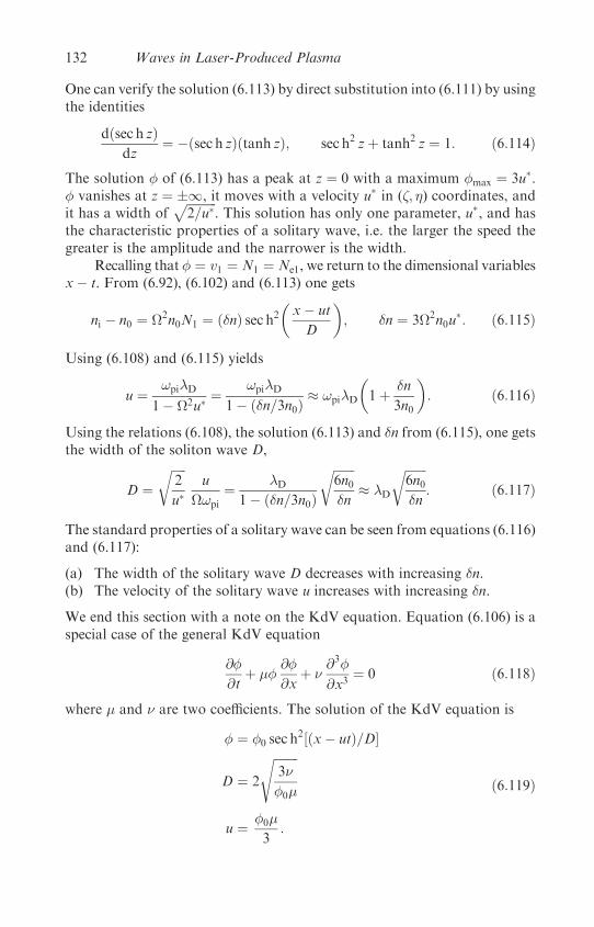
One can verify the solution (6.113) by direct substitution into (6.111) by usingthe identities

dðsec h zÞdz

¼ �ðsec h zÞðtanh zÞ; sec h2 zþ tanh2 z ¼ 1: ð6:114Þ

The solution � of (6.113) has a peak at z ¼ 0 with a maximum �max ¼ 3u�.� vanishes at z ¼ �1, it moves with a velocity u� in (�; ) coordinates, andit has a width of

ffiffiffiffiffiffiffiffiffiffi2=u�

p. This solution has only one parameter, u�, and has

the characteristic properties of a solitary wave, i.e. the larger the speed thegreater is the amplitude and the narrower is the width.

Recalling that � ¼ v1 ¼ N1 ¼ Ne1, we return to the dimensional variablesx� t. From (6.92), (6.102) and (6.113) one gets

ni � n0 ¼ �2n0N1 ¼ ð�nÞ sec h2�x� ut

D

�; �n ¼ 3�2n0u

�: ð6:115Þ

Using (6.108) and (6.115) yields

u ¼!piD

1� �2u�¼

!piD1� ð�n=3n0Þ

� !piD

�1þ �n

3n0

�: ð6:116Þ

Using the relations (6.108), the solution (6.113) and �n from (6.115), one getsthe width of the soliton wave D,

D ¼ffiffiffiffiffi2

u�

ru

�!pi

¼ D1� ð�n=3n0Þ

ffiffiffiffiffiffiffi6n0�n

r� D

ffiffiffiffiffiffiffi6n0�n

r: ð6:117Þ

The standard properties of a solitary wave can be seen from equations (6.116)and (6.117):

(a) The width of the solitary wave D decreases with increasing �n.(b) The velocity of the solitary wave u increases with increasing �n.

We end this section with a note on the KdV equation. Equation (6.106) is aspecial case of the general KdV equation

@�

@tþ ��

@�

@xþ �

@3�

@x3¼ 0 ð6:118Þ

where � and � are two coefficients. The solution of the KdV equation is

� ¼ �0 sec h2½ðx� utÞ=D�

D ¼ 2

ffiffiffiffiffiffiffiffi3�

�0�

s

u ¼ �0�

3:

ð6:119Þ


In our equation (6.106) the coefficients are � ¼ 1 and � ¼ 12, implying �0 ¼ 3u

and D ¼ ð2=uÞ1=2 (see equation (6.113)).The soliton concept has also attracted interest and speculation in laser–

plasma interactions. In particular the solitary waves were associated with theponderomotive force. Cavity structures, measured experimentally nearthe critical surface, were related to solitary waves. However, it seems thatthe very interesting phenomena of the soliton have not yet been fully andsuccessfully investigated in laser–plasma interactions.

A Soliton Wave 133

Chapter 7

Laser-Induced Electric Fields in Plasma

7.1 High- and Low-Frequency Electric Fields

In laser–plasma interaction the electric field, or rather the various macro-scopic electric fields, plays a major role in defining the properties of theplasma system. First, the laser electric field, EL cos!Lt, is propagating intothe plasma, where part of it is reflected and the other part is absorbed. Thelaser electric field amplitude and its frequency are given by

EL ðV=cmÞ ¼ 2:75� 109�

IL

1016 W=cm2

�1=2

!L ðs�1Þ ¼ 2�c

�L¼ 1:88� 1015

�mm�L

� ð7:1Þ

where IL is the laser energy flux and �L is the laser wavelength. !L sets thescale for high-frequency phenomena and the period of one laser oscillationð2�=!LÞ is about 3.3 fs for a 1 mm laser wavelength.

The propagating and reflected electric fields in different plasma mediawere calculated in chapter 5. The electric fields associated with the possiblewaves in the plasma were calculated in chapter 6. Two classes of electricfields were derived: the high-frequency one, of the order of the laserfrequency or the electron–plasma frequency, ! � !pe � 1015 s�1 (forelectron density �1021 cm�3), and the low-frequency electric field of theorder of the ion–plasma frequency ! � 1012 s�1. The appropriate timescales are about 1 fs for the high-oscillation fields and about 1 ps for thelow-oscillation fields.

Another interesting case of a slowly-varying (in time) electric field isthe one induced by the ponderomotive force and developed in chapter 4.This ‘d.c.’ (i.e. very slow varying in time) electric field E is in the directionof the gradient of E2

L and the magnitude of this electric field (E) is of

134

the order

eneE ��!2pe

!2L

�E2L

16�rL

) E ðV=cmÞ � 1:0� 107�

IL

1016 W=cm2

��1021 cm�3

nec

��100 mm

rL

�ð7:2Þ

where ne is the electron density, nec is the electron critical density, rL is thelaser radius defined by IL � expð�r2=2r2LÞ, and it is assumed thatgradE2

L � E2L=rL. As discussed in chapter 6, an electric field can also be

induced by the ponderomotive forces associated with the wave–waveinstabilities.

In general, the electric field in laser–plasma interactions is discussed inthe previous three chapters. In this chapter we shall add two cases ofslowly varying electric fields: in section 7.2 the electric field of an expandingplasma into the vacuum is calculated and in section 7.3 an electric field in thedouble layers is calculated. An example of charge particle acceleration due tothese electric fields is given in section 7.4.

7.2 Expansion of Plasma into the Vacuum

A laser-created plasma is expanding into the vacuum, towards the laserirradiation (Gurevich et al. 1965, 1968, 1969, Crow et al. 1975, Anisimovet al. 1979, Sigel 1979). When a laser irradiates a target, the electrons areheated and they expand towards the vacuum. The ions follow the electronsthat expand towards the vacuum. In this section the hydrodynamic problemof plasma expansion is calculated, by assuming that the electrons and theions are treated as separate fluids with different temperatures.

We assume the simplest one-dimensional problem with plane geometry.For a laser spot on target 2rL ¼ D (rL, the laser radius, is defined in the previoussection), this approximation is valid as long as D � vit, where vi is the stream-ing velocity of the ions and t is the expansion time. The continuity equation forthe ions and the momentum equations for the electrons and ions are

@ni@t

þ @ðniviÞ@x

¼ 0

@P

@xþ eneE ¼ 0

mini

�@vi@t

þ vi@vi@x

�¼ eZniE

ð7:3Þ

where E is the electric field in the expanding plasma, ni and ne are the ion andelectron densities accordingly, mi is the ion mass and Ze is the ion charge.

Expansion of Plasma into the Vacuum 135

Neglecting the ion temperature in comparison with the electron temperatureTe, the plasma pressure P is given by

P ¼ nekBTe: ð7:4Þ

In the electron momentum equation, the second equation of (7.3), the inertiaterm of the electrons (me dve=dt, where ve is the electron fluid velocity) isneglected. This is justified when adding the two inertia terms of the electronsand the ions, since me � mi, and neglecting the high-frequency oscillations(not relevant to this problem) one has dve=dt � dvi=dt. Assuming chargeneutrality ne ¼ Zni, adding the electron and ion momentum equations of(7.3), one gets

@vi@t

þ vi@vi@x

¼ � 1

mini

@P

@x: ð7:5Þ

Using the definition of the sound velocity, ne ¼ Zni; and equation (7.4), onegets

c2s ¼1

mi

@P

@ni¼ ZkBTe

mi

ð7:6Þ

where the electron temperature is assumed constant, a reasonable assump-tion for the plasma corona under investigation. Implying the identity@P=@x ¼ ð@P=@nÞð@n=@xÞ into the right-hand side of equation (7.5) andusing (7.6), we obtain

@vi@t

þ vi@vi@x

þ c2s

�1

ni

@ni@x

�¼ 0: ð7:7Þ

One has to solve (7.7) together with the continuity equation (first of equa-tions (7.3)). For this purpose we define the dimensionless variables

� ¼ x

cst; v ¼ vi

cs; n ¼ ni

n0

@

@x¼ 1

cst

@

@�;

@

@t¼ � �

t

@

@�

ð7:8Þ

where n0 is the background density. Substituting (7.8) into the first equationof (7.3) and (7.7), we get

v� � 1

1 v� �

� �d ln n=d�

dv=d�

� �¼

0

0

� �: ð7:9 Þ

The determinant of the 2� 2 matrix should vanish in order to get a nonzerosolution, yielding

v ¼ � þ 1 ) vi ¼x

tþ cs ð7:10Þ

136 Laser-Induced Electric Fields in Plasma

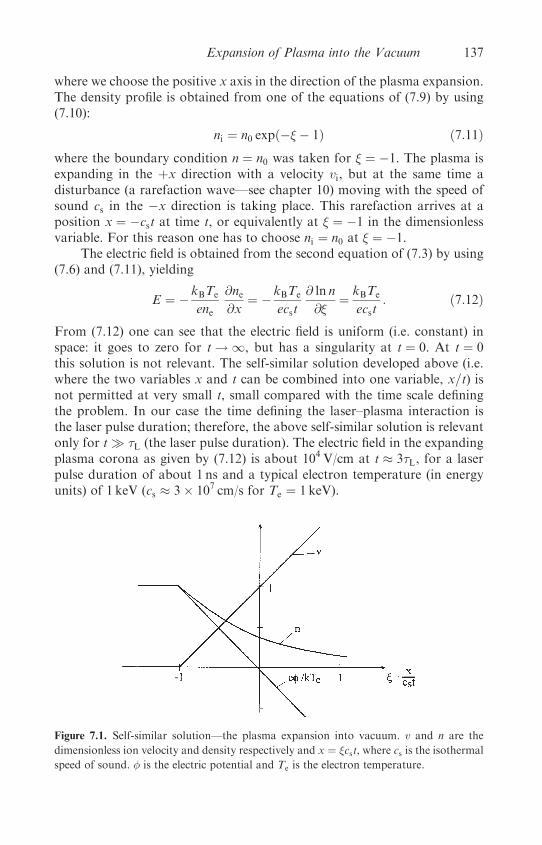
where we choose the positive x axis in the direction of the plasma expansion.The density profile is obtained from one of the equations of (7.9) by using(7.10):

ni ¼ n0 expð�� 1Þ ð7:11Þwhere the boundary condition n ¼ n0 was taken for � ¼ �1. The plasma isexpanding in the þx direction with a velocity vi, but at the same time adisturbance (a rarefaction wave—see chapter 10) moving with the speed ofsound cs in the �x direction is taking place. This rarefaction arrives at aposition x ¼ �cst at time t, or equivalently at � ¼ �1 in the dimensionlessvariable. For this reason one has to choose ni ¼ n0 at � ¼ �1.

The electric field is obtained from the second equation of (7.3) by using(7.6) and (7.11), yielding

E ¼ � kBTe

ene

@ne@x

¼ � kBTe

ecst

@ ln n

@�¼ kBTe

ecst: ð7:12Þ

From (7.12) one can see that the electric field is uniform (i.e. constant) inspace: it goes to zero for t ! 1, but has a singularity at t ¼ 0. At t ¼ 0this solution is not relevant. The self-similar solution developed above (i.e.where the two variables x and t can be combined into one variable, x=t) isnot permitted at very small t, small compared with the time scale definingthe problem. In our case the time defining the laser–plasma interaction isthe laser pulse duration; therefore, the above self-similar solution is relevantonly for t � �L (the laser pulse duration). The electric field in the expandingplasma corona as given by (7.12) is about 104 V/cm at t � 3�L, for a laserpulse duration of about 1 ns and a typical electron temperature (in energyunits) of 1 keV (cs � 3� 107 cm/s for Te ¼ 1 keV).

Figure 7.1. Self-similar solution—the plasma expansion into vacuum. v and n are the

dimensionless ion velocity and density respectively and x ¼ �cst, where cs is the isothermal

speed of sound. � is the electric potential and Te is the electron temperature.

Expansion of Plasma into the Vacuum 137

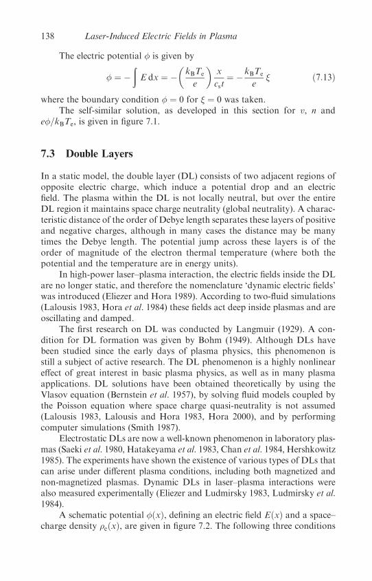
The electric potential � is given by

� ¼ �ðE dx ¼ �

�kBTe

e

�x

cst¼ � kBTe

e� ð7:13Þ

where the boundary condition � ¼ 0 for � ¼ 0 was taken.The self-similar solution, as developed in this section for v, n and

e�=kBTe, is given in figure 7.1.

7.3 Double Layers

In a static model, the double layer (DL) consists of two adjacent regions ofopposite electric charge, which induce a potential drop and an electricfield. The plasma within the DL is not locally neutral, but over the entireDL region it maintains space charge neutrality (global neutrality). A charac-teristic distance of the order of Debye length separates these layers of positiveand negative charges, although in many cases the distance may be manytimes the Debye length. The potential jump across these layers is of theorder of magnitude of the electron thermal temperature (where both thepotential and the temperature are in energy units).

In high-power laser–plasma interaction, the electric fields inside the DLare no longer static, and therefore the nomenclature ‘dynamic electric fields’was introduced (Eliezer and Hora 1989). According to two-fluid simulations(Lalousis 1983, Hora et al. 1984) these fields act deep inside plasmas and areoscillating and damped.

The first research on DL was conducted by Langmuir (1929). A con-dition for DL formation was given by Bohm (1949). Although DLs havebeen studied since the early days of plasma physics, this phenomenon isstill a subject of active research. The DL phenomenon is a highly nonlineareffect of great interest in basic plasma physics, as well as in many plasmaapplications. DL solutions have been obtained theoretically by using theVlasov equation (Bernstein et al. 1957), by solving fluid models coupled bythe Poisson equation where space charge quasi-neutrality is not assumed(Lalousis 1983, Lalousis and Hora 1983, Hora 2000), and by performingcomputer simulations (Smith 1987).

Electrostatic DLs are now a well-known phenomenon in laboratory plas-mas (Saeki et al. 1980, Hatakeyama et al. 1983, Chan et al. 1984, Hershkowitz1985). The experiments have shown the existence of various types of DLs thatcan arise under different plasma conditions, including both magnetized andnon-magnetized plasmas. Dynamic DLs in laser–plasma interactions werealso measured experimentally (Eliezer and Ludmirsky 1983, Ludmirsky et al.1984).

A schematic potential �ðxÞ, defining an electric field EðxÞ and a space–charge density �eðxÞ, are given in figure 7.2. The following three conditions


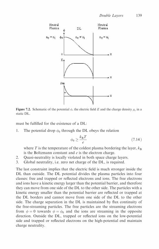
must be fulfilled for the existence of a DL:

1. The potential drop �0 through the DL obeys the relation

�0 �kBT

eð7:14 Þ

where T is the temperature of the coldest plasma bordering the layer, kBis the Boltzmann constant and e is the electron charge.

2. Quasi-neutrality is locally violated in both space charge layers.3. Global neutrality, i.e. zero net charge of the DL, is required.

The last constraint implies that the electric field is much stronger inside theDL than outside. The DL potential divides the plasma particles into fourclasses: free and trapped or reflected electrons and ions. The free electronsand ions have a kinetic energy larger than the potential barrier, and thereforethey can move from one side of the DL to the other side. The particles with akinetic energy smaller than the potential barrier are reflected or trapped atthe DL borders and cannot move from one side of the DL to the otherside. The charge separation in the DL is maintained by flux continuity ofthe free-streaming particles. The free particles are the streaming electronsfrom � ¼ 0 towards � ¼ �0 and the ions are streaming in the oppositedirection. Outside the DL, trapped or reflected ions on the low-potentialside and trapped or reflected electrons on the high-potential end maintaincharge neutrality.

Figure 7.2. Schematic of the potential �, the electric field E and the charge density �e in a

static DL.

Double Layers 139

In the next section it is shown how these DLs can accelerate electronsand ions.

7.4 Charged Particle Acceleration

7.4.1 A static model

Laser-produced plasma experiments have shown that high-energy ions areemitted and carry away a large fraction of the absorbed laser energy. X-rayemission measurements at laser intensities IL�

2L > 1014 Wmm2/cm2 (the laser

irradiance IL is measured in W/cm2 and the laser wavelength �L in mm)have shown non-Maxwellian electron velocity distribution (Haines 1979,Ahlstrom 1982). Two distinct electron temperatures, the so-called thermal(or cold) and supra-thermal (or hot) temperatures, usually characterize thisdistribution. These electron distributions are associated with the existence offast ions. We shall now describe a very simple model showing how DLsaccelerate ions.

A high-power laser irradiates a spherical pellet of radiusR. The fast elec-trons emitted from the spherical plasma leave the sphere until an electrostaticpotential is set up to stop the outgoing electrons. The thermal electrons thentraverse this field (i.e. the DL), decelerate and accelerate back towards thesphere. The same field will accelerate positive ions from the outer surfaceof the plasma. The fast ions are field-extracted from the plasma and thereforethey can be used to measure the electric field and the potential of the DLunder consideration. For simplicity, monochromatic fast electrons andprotons (the ions) species are assumed. The protons, with a mass M, areemitted from the DL with velocity v, so that

12Mv2 ¼ e� ð7:15Þ

where � is the DL potential drop. Assuming that the fast protons have a totalenergy W and a total charge Q, one can write

W ¼ Q�: ð7:16Þ

The charge of the proton q present at any moment inside the DL (defined bythe potential drop � and charge separation d) is given by

q ¼ Qd

v�L¼ Wd

�v�Lð7:17Þ

where �L is the laser pulse duration. For the geometry under consideration,the DL can be modelled by a capacitor with a capacity C:

C ¼ 4�R2

d: ð7:18Þ


The capacitor is charged with a charge greater than q (the momentary chargeof the protons inside the DL) and with a voltage equal to �; therefore

� >q

C¼ Wd2

4�R2�v�L: ð7:19Þ

This relation implies that the electric field created by the charge separation(i.e. the DL) is

E ¼ �

d�

�W

4�R2v�L

�1=2: ð7:20Þ

The velocity of the ions is measured from the time of flight and the number ofions is measured with charge collectors, and from these their energy isdeduced. Using a typical experiment where W ¼ 10 J, v ¼ 108 cm/s,�L ¼ 1 ns, R ¼ 50 mm, one gets an electric field E > 5� 108 V/cm.

From this simple model we can conclude that the fast electrons transfertheir energy to the electrostatic field in order to create a DL, while the fastions take their energy from the electric field of the DL. This mechanismcan lead to very high electric fields, as is obtained above.

7.4.2 A dynamic model

DL solutions have been obtained theoretically by solving a two-fluid modelcoupled by the Poisson equation, where space-charge quasi-neutrality is notassumed. For example, in the simulation (Hora et al. 1984) of the interactionbetween a plasma with a highly bent parabolic initial density profile of 25wavelengths thickness and a neodymium glass laser radiation of 1017 W/cm2

intensity, the following results were achieved:

(a) a caviton (i.e. a minimum in the density) is created,(b) the plasma is accelerated towards the vacuum with a velocity of about

108 cm/s,(c) a dynamic (time-dependent) DL is created with a maximum electric field

about 109 V/cm and(d) electrons were accelerated to energies �140 keV.

The following simple dynamical model has been suggested in order to explainhow dynamical DL accelerates electrons (Eliezer et al. 1995).

We assume that a DL is created at time t ¼ 0 during a very short timeinterval, described by the Dirac delta function, �ðtÞ. The Poisson equationgives

dE

dx¼ �4�e½neðx; tÞ � niðx; tÞ� ¼ f ðxÞ�ðtÞ: ð7:21Þ

Charged Particle Acceleration 141

Integrating this equation yields

E ¼ �ðtÞðf ðxÞ dx ¼ FðxÞ�ðtÞ: ð7:22Þ

For example, from a ‘quadrupole’ type (two DL in a sequence) of interactiondefined by a charge density

f ðxÞ ¼ K

�2x

�4

�1� 2x2

�2

��exp

�� x2

�2

�ð7:23Þ

one gets a space-dependent electric field

FðxÞ ¼ K

�2

�1þ 2x2

�2

�exp

�� x2

�2

�: ð7:24Þ

The Newton equation for the electron

dv

dt¼ � eE

m¼ � e

mFðxÞ�ðtÞ ð7:25Þ

has the solution

dx

dt¼ vðtÞ ¼ � e

mFðxÞðtÞ þ v0 ¼ ðv1 � v0ÞðtÞ þ v0

ðtÞ ¼1 for t > 0

0 for t < 0

( ð7:26Þ

where v0 is the initial velocity and v1 the final velocity, after the acceleration.If the electron is at the position x when the force is applied (at t ¼ 0 in thisexample), then the final velocity is achieved according to the value of�eFðxÞ=m.

The position of the electron is given by integrating (7.26):

xðtÞ ¼ v0tþ ðv1 � v0ÞðtÞt ð7:27Þwhere the identity �ðtÞt ¼ 0 was used.

Substituting (7.26) into (7.25), the electric field can be written

Eðx; tÞ ¼ FðxÞ�ðtÞ ¼ �m

eðv1 � v0Þ�ðtÞ: ð7:28Þ

The energy given to the particle by the electric field is given by using (7.26)and (7.28):

�e

ðEðx; tÞ dx ¼ � e

ðþ1

�1E½xðtÞ; t� dx

dtdt

¼ mðv1 � v0Þðþ1

�1�ðtÞ½ðv1 � v0ÞðtÞ þ v0� dt

¼ 12mðv21 � v20Þ ð7:29Þ


where in the last stage we have used the identityððtÞ�ðtÞ dt ¼ 1

2 ð7:30Þ

which can be easily proven by integrating by parts.Equation (7.29) is the energy conservation, which shows that a particle

can be accelerated or decelerated by E, depending on the value of the electricfield at the particle position, at the time that the DL is created. It has beenshown that under the right configuration a charged particle can be acceler-ated to high energies even when the electric field is changing very fast in time.

In summary, it has been demonstrated that a dynamic DL can acceleratecharged particles, as was suggested in astrophysics (Falthammer 1987,Alfven 1988, Raadu 1989). The existence of DL in laser-produced plasmain the outer corona was detected directly by the deflection of a probingbeam (Ehler 1975, Mendel and Olsen 1975) and by using Rogowski coils(Eliezer and Ludmirsky 1983). Therefore, similar to DL in astrophysics,the DL might play an important role in laser–plasma interactions.

Charged Particle Acceleration 143

Chapter 8

Laser-Induced Magnetic Fields in Plasma

When a laser irradiates a medium, the laser magnetic field BL cos!Lt (togetherwith the associated electric field) is propagating into the plasma, part of it isreflected and the other part is absorbed. The laser magnetic field amplitudeand its frequency are given by

BLðGaussÞ ¼ 9:2� 106�

IL

1016 W=cm2

�1=2

!L ðs�1Þ ¼ 2�c

�L¼ 1:88� 1015

�mm�L

� ð8:1Þ

where IL is the laser energy flux and �L is the laser wavelength. !L sets thescale for high-frequency phenomena. The period of one laser oscillation(2�=!L) is about 3.3 fs for a laser with a wavelength of 1 mm. The propagationof electromagnetic field in plasma was calculated in chapter 5. There are alsohigh-frequency magnetic fields associated with the stimulated Brillouin andRaman scattering discussed in chapter 6.

In this chapter we are interested only in the slowly-varying (on the timescale of the laser pulse duration) magnetic fields, approximated as d.c.magnetic fields. The generation of d.c. mega-Gauss magnetic fields inlaser-produced plasmas is well-documented (Stamper et al. 1971, Boyd andCooke 1988, Horovitz et al. 1998). In this chapter we discuss the mechanismsproposed to explain the generation of the d.c. magnetic fields and sometheoretical consequences.

In section 8.1, the rn�rT toroidal magnetic field (Raven et al. 1978,Bobin 1985, Stamper 1991) is derived. In section 8.2, the magneto-hydrodynamic equations are derived (Braginskii 1965, Nicholson 1983,Parks 1991). Using the generalized Ohm’s law together with theMaxwell equa-tions, a generalized equation for the d.c.magnetic field is obtained. Inparticularthe magnetic Reynolds number is defined and the dynamo effect is described(Briand et al. 1983, Dragila 1987). Section 8.3 describes the Faraday effect

144

and the magnetic field created by the inverse Faraday effect (Steiger andWoods 1972, Eliezer et al. 1992, Lehner 1994, 2000, Sheng and Meyer-ter-Vehn 1996, Haines 2001). In section 8.4 we develop the dispersion relationfor waves in the presence of the d.c. magnetic field. In particular, ordinary,extraordinary and Alfven waves are analysed. We conclude this chapterwith section 8.5, showing the effect of resonance absorption in the presenceof the d.c. magnetic field (Woo et al. 1978, David and Pellat 1980).

8.1 The rn�rT Toroidal Magnetic Field

One can see from the Maxwell equation (in Gaussian units)

r� E ¼ � 1

c

@B

@tð8:2Þ

that a magnetic field is generated if the electric field E does not have avanishing curl, i.e. the electric field in the plasma is not derivable from apotential. As discussed in the previous chapter, the electric field in theplasma is required in order to keep quasi-neutrality on a large scale(compared with the Debye length) during long periods of time (comparedwith the inverse plasma frequency). From the electron momentum equation(see section 3.1), on the long time scale it is justifiable to neglect the inertia ofthe electrons, implying

0 ¼ �rPe � eneE: ð8:3Þ

This equation is equivalent to the assumption that the volume forces due tothe free electrical charges balance the electron pressure gradient. In equation(8.3), the charge motion is neglected. Substituting the ideal gas equation ofstate

Pe ¼ nekBTe ð8:4Þ

into equation (8.3), one gets the electric field E for equation (8.2), yielding

@B

@t¼ ckB

enerTe �rne: ð8:5Þ

From this equation an estimate of the magnitude of the magnetic field B isobtained by the substitution of

@

@t� 1

�L;

rnene

� 1

Ln

; rTe �Te

LT

ð8:6Þ

into equation (8.5), implying

B ðMGaussÞ � 10

��L1 ns

��kBTe

1 keV

��30 mmLn

��30 mmLT

�ð8:7Þ

The rn�rT Toroidal Magnetic Field 145

where �L is the laser pulse duration or the characteristic loss time due toablation and diffusion.

Thus a magnetic field is generated from non-parallel density andtemperature gradients, as shown in figure 8.1. It turns out that this is thedominant phenomenon for the generation of a toroidal magnetic field,although there are other terms that contribute to the generation of d.c.toroidal magnetic fields, as proven in the following section.

8.2 Magneto-Hydrodynamics and the Evolution of

the Magnetic Field

In this section the evolution equation of the magnetic field is developed. Forthis purpose the plasma is described as a magnetic fluid and the equationsinclude the generalized Ohm’s law, together with Maxwell equations. Thefollowing equations describe the mass conservation and the momentumconservation for the ion and electron fluids (in Gaussian units):

@ni@t

þr � ðniviÞ ¼ 0

@ne@t

þr � ðneveÞ ¼ 0

mini@vi@t

þminiðvi � rÞvi ¼ �rPi þ Zeni

�Eþ vi � B

c

�þ Ri

mene@ve@t

þmeneðve � rÞve ¼ �rPe � ene

�Eþ ve � B

c

�þ Re

ð8:8Þ

wheremi,me and ni, ne are the ion and electron masses and densities, vi and veare the ion and electron fluid velocities, Pi and Pe are the appropriatepressures, E and B are the electric and magnetic fields in the plasma

Figure 8.1. Magnetic field is generated from non-parallel density and temperature gradients.

146 Laser-Induced Magnetic Fields in Plasma

medium and c is the light velocity. ReðrÞ represents the change in electronmomentum at position r due to collisions with ions and RiðrÞ is the changein ion momentum at r due to collisions with electrons. Therefore

Re ¼ �Ri: ð8:9Þ

We combine the ion and the electron equations to obtain the equations forone fluid. This fluid is described by the mass density �ðrÞ, charge density�eðrÞ, a centre of mass fluid flow u and an electrical current J, defined by

� ¼ mini þmene ffi mini

�e ¼ Zeni � ene

u ¼ 1

�ðminivi þmeneveÞ

J ¼ Zenivi � eneve

ð8:10Þ

and a total pressure

P ¼ Pe þ Pi : ð8:11Þ

Multiplying the first equation of (8.8) by mi and the second equation byme and adding, one gets the one-fluid continuity equation (i.e. the massconservation):

@�

@tþr � ð�uÞ ¼ 0: ð8:12Þ

Multiplying the first equation of (8.8) by Ze and the second equation by �eand adding, one gets the charge continuity, or the charge conservation law:

@�e@t

þr � J ¼ 0: ð8:13Þ

It is assumed that ve, vi, @ne=@t and @ni=@t are small quantities and second-order terms, such as ðv � rÞv, are neglected. Adding the third equation of(8.8) with the fourth equation and using the definitions (8.10) and (8.11),one gets the one-fluid force equation (or the momentum conservation):

�@u

@t¼ �rPþ �eEþ 1

cJ� B: ð8:14Þ

8.2.1 The generalized Ohm’s law

We assume charge neutrality

ne ¼ Zni ð8:15Þand neglect the second-order terms (in ve, vi, @ne=@t and @ni=@t) and1=mi � 1=me. Adding the third equation of (8.8) multiplied by Ze=mi with

Magneto-Hydrodynamics and the Evolution of the Magnetic Field 147

the fourth equation multiplied by �e=me, and using the definitions (8.10),one gets

@J

@t¼ e

me

r��

1þ Ti

ZTe

��1

P

�

þ Ze2�

memi

�Eþ 1

cu� B

�� e

mecJ� Bþ e

me

Ri : ð8:16Þ

Algebraic relations such as the following were used in order to deriveequation (8.16):

e2neme

¼ e2Znime

¼ e2Z

memi

ðminiÞ ffie2Z

memi

ðmini þmeneÞ ¼e2Z�

memi

ð8:17Þ

e2nevemec

¼ e

mecðeneve � ZeniviÞ þ

Ze2nimivi

memic

ffi � e

mecJþ Ze2

memicðnimivi þ nemeveÞ ¼ � e

mecJþ Ze2

memic�u ð8:18Þ

Ze

mi

Ri �e

me

Re ¼�Ze

mi

þ e

me

�Ri ffi

e

me

Ri ð8:19Þ

Pe

P¼ nekBTe

nekBTe þ nikBTi

¼ ZniTe

ZniTe þ niTi

¼�1þ Ti

ZTe

��1

ð8:20Þ

where Ri in equation (8.16) is the change in the ion momentum due tocollisions with electrons. Therefore, one can expand Ri as a Taylor seriesin the relative velocity between the ions and the electrons. Keeping onlythe first term in the Taylor expansion, one gets

Ri ¼ C1ðvi � veÞ: ð8:21ÞUsing charge neutrality and the definition of the electric current, equations(8.10) and (8.15), into equation (8.21) gives

Ri ¼ C2J: ð8:22Þ

Since the value of C2 does not depend on the general structure of equation(8.16), one can consider this equation for the following special case: steadystate, no pressure (or temperature) gradients and without magnetic field.Substituting (8.22) into (8.16) for this special case, one obtains

Ze�

mi

Eþ C2J ¼ 0: ð8:23Þ

Using now the simple Ohm’s law for this case (see section 2.3), where �E is theelectrical conductivity coefficient,

J ¼ �EE ð8:24Þ


one gets the value of C2, implying

Ri ¼ C2J ¼ � Ze�

mi�EJ: ð8:25Þ

Substituting (8.25) into (8.16), we get the generalized Ohm’s law:�memi

Ze2�

�@J

@t¼

�mi

Ze�

�r��

1þ Ti

ZTe

��1

P

�þ Eþ

�1

c

�u� B

��

mi

Zec�

�J� B�

�1

�E

�J: ð8:26Þ

The magneto-hydrodynamic equations are (8.12), (8.13), (8.14) and (8.26),together with the following Maxwell equations:

r� E ¼ ��1

c

�@B

@t; r� B ¼

�4�

c

�Jþ

�1

c

�@E

@t: ð8:27Þ

One therefore has 14 equations with 14 unknowns: �, �E, u, J, E and B. Thisis correct only if the temperatures Te and Ti are known, otherwise the (elec-tron and ion) energy conservation equations are also necessary. Moreover,knowledge of the equations of state, Pe ¼ Peð�;TeÞ and Pi ¼ Pið�;TiÞ, isnecessary. For not very dense plasmas (�� solid), the ideal gas equationsof state are suitable (such as those we have used in equation (8.20)).

In this chapter we are interested in calculating the steady-state magneticfield. Therefore, the generalized Ohm’s law given in equation (8.26) isassumed, together with the assumption @J=@t ¼ 0, yielding an electric field

E ¼�

1

�E

�J�

�mi

Ze�

�r��

1þ Ti

ZTe

��1

P

�

��1

c

�u� Bþ

�mi

Zec�

�J� B: ð8:28Þ

From this equation we see that the electric field in the plasma has fourcontributions:

1. The J� B term, which is the Hall effect.2. u� B is the convective (plasma flow) term.3. rP is the pressure gradient contribution.4. The J=�E term is the (standard Ohm’s law) voltage drop on plasma-

active resistance.

Using for the electrical conductivity the value obtained in section 2.3 (Drudemodel),

�E ¼ e2neme�ei

ð8:29Þ


and substituting (8.28) into the first equation of (8.27), one gets for Ti � Te

@B

@t¼ �mec�ei

e2r�

�J

ne

�

þ ckBene

rTe �rne þr� ðu� BÞ � 1

er�

�J� B

ne

�: ð8:30Þ

The first term in (8.30) may contribute a toroidal magnetic field, as describedin figure 8.2. The second term is the one given in the previous section anddescribed schematically in figure 8.1.

The current J is substituted into (8.30) from the second equation of(8.27), and using the first equation of (8.27) one obtains a complex equationfor the magnetic field generated in laser–plasma interaction. We considernow some special cases.

Case 1

It is assumed that the second and third terms of equation (8.30) are domi-nant. Looking for a d.c. solution (@B=@t ¼ 0), one gets from equation (8.30):

c

enerPe þ u� B ¼ 0: ð8:31Þ

Taking r � 1=L and u � cs, where L is the scale length of the electron pres-sure gradient and cs is the speed of sound, and using the ideal gas equation ofstate for the electron pressure (equation (8.4)), one gets from equation (8.31):

B ��

c

cs

�ðkBTe=eÞ

L� ðmic

2kBTeÞ1=2

eL

��mi

mp

�1=2� Te

keV

�1=2� 30 mmL

�½MGauss� ð8:32Þ

where mi and mp are the ion and the proton masses respectively. For anelectron temperature of 1 keV and a pressure scale length of 30 mm onegets a d.c. magnetic field of 1MG.

Figure 8.2. A toroidal magnetic field created by a return current.


Case 2

It is now assumed that the first and third terms of equation (8.30) aredominant.

Moreover, a constant electrical conductivity is taken so that equation(8.30) can be rewritten as (after using equation (8.29))

@B

@t¼ � c

�Er� Jþr� ðu� BÞ: ð8:33Þ

Substituting into this equation the second equation of (8.27) with @E=@t ¼ 0,one obtains the equation for the magnetic field:

@B

@t¼ � c2

4��Er� ðr � BÞ þ r � ðu� BÞ: ð8:34Þ

Using the identity

r� ðr � BÞ ¼ �r2Bþrðr � BÞ ¼ �r2

B ð8:35Þ(where theMaxwell equationr � B ¼ 0 is used), one gets from equation (8.34):

@B

@t¼

�c2

4��E

�r2

Bþr� ðu� BÞ: ð8:36Þ

8.2.2 The magnetic Reynolds number

The first term on the right-hand side of (8.36) describes the diffusion of themagnetic field, while the second term is the convection of the plasma fluidmoving with a velocity u (relative to a fixed observer, the laboratory frameof reference). The ratio between the convective and the diffusion termsdefines the magnetic Reynolds number Rm:

Rm ¼�

uB=L

ðc2BÞ=ð4��EL2Þ

�¼ 4�

c2

��ELu

�ð8:37Þ

where L is the macroscopic scale length and u is the characteristic flowvelocity. Note that Rm is dimensionless (in the Gaussian units used herethe electrical conductivity coefficient �E has dimensions of s�1). c2=ð4��EÞis equivalent to the kinematic viscosity in defining the Reynolds numberfor a fluid flow (¼ inertial force/viscous force).

8.2.3 Magnetic Reynolds numbers Rm � 1

For Rm � 1 the convective term is negligible and equation (8.36) describesthe diffusion of the magnetic field

@B

@t¼ �r2B; � � c2

4��E: ð8:38Þ


This equation is similar to the heat diffusion equation

@T

@t¼ �r2T ð8:39Þ

where T is the temperature and � is the coefficient of heat conduction.Similarly, in a viscous fluid flow the vorticity � satisfies a similar equation:

@�

@t¼ �r2�; � � r� u ð8:40Þ

where � is the kinematic viscosity. Note that �, � and � have the dimension ofcm2/s in c.g.s. and m2/s in m.k.s.

We now analyse equation (8.38). Assuming at t ¼ 0 (initial condition) amagnetic field Biðr; 0Þ in Cartesian coordinates (i ¼ x; y; z), then at t > 0 themagnetic field is given by

Biðr; tÞ ¼ðd3r0Gðr� r

0; tÞBiðr0; 0Þ ð8:41Þ

where Gðr� r0; tÞ is Green’s function:

Gðr� r0; tÞ ¼ 1

ð4��tÞ3=2exp

�� ðr� r

0Þ2

4�t

�: ð8:42Þ

This solution shows that the magnetic field at an initial position r0 diffuses

in time with a Gaussian profile which has the width ð4�tÞ1=2, i.e. the widthincreases with the square root of time. An estimate of the magnetic fielddiffusion time is derived by taking r2 � 1=L2 in equation (8.38), yielding

@B

@t� �

L2B: ð8:43Þ

The solution of this equation is

B ¼ B0 exp

� t

�m

�; �m ¼ L2

�¼ 4��EL

2

c2¼ RmL

u: ð8:44Þ

The þ or � sign refer to ‘gain’ or ‘loss’ (with time) of the magnetic field.For example, in a typical laser-produced plasma where diffusion is

dominant, one has L � 100 mm and u � 106 cm/s, implying a magneticReynolds number Rm � 0:1 and a diffusion relaxation time �m � 1 ns.

8.2.4 Magnetic Reynolds numbers Rm 1

For Rm 1 the diffusion term is negligible and equation (8.36) describes theconvection of the magnetic field:

@B

@t¼ r� ðu� BÞ: ð8:45Þ


In this case it is important to notice that if initially there is a magnetic field inthe x–y plane, B ¼ ðBx;By;Bz ¼ 0Þ, then equation (8.45) implies that fort > 0 a magnetic field perpendicular to the x–y plane is induced. Forexample,

t ¼ 0 : B ¼ ðBx;By; 0Þ; u ¼ ð0; 0; uÞ

t > 0 :@Bz

@t¼@ðuByÞ@x

) Bzðt > 0Þ � tu

LByðt ¼ 0Þ:

ð8:46Þ

Assuming that in laser–plasma interactions ripples are created of theorder of L ¼ 10 mm and the plasma flow towards the laser is u ¼ 106 cm/s,then at a time t � �L, where �L � 1 ns is the laser pulse duration, one getsfrom (8.46)

Bzðt � �LÞ � Byðt ¼ 0Þ: ð8:47Þ

This phenomenon, where a magnetic field in the x–y plane develops into amagnetic field in the z direction, is called the dynamo effect. Therefore, wehave seen that for a large magnetic Reynolds number the toroidal magneticfield may develop into a large axial magnetic field. However, for thisphenomenon to happen fluctuations of small-scale L are necessary. Thus,this effect is a random process.

In the next section we shall see how an axial magnetic field (bydefinition, in the direction of the laser irradiation, or normal to the planetarget) can be created in a controllable way for any magnetic Reynoldsnumbers.

8.3 Faraday and Inverse Faraday Effects

8.3.1 The Faraday effect

Michael Faraday discovered in 1845 that when plane-polarized light passedthrough lead glass in the direction of a magnetic field, the plane ofpolarization was rotated. The linear polarized electric field rotates whenpropagating along the magnetic field in a dielectric or a plasma medium. Alinear polarized wave can be resolved into the sum of left- and right-circularlypolarized waves, and the rotation arises due to the difference in the index ofrefraction between the two waves. The angle of rotation is proportional tothe magnitude of the magnetic field.

We now calculate the angle of rotation for a linearly polarized lightpropagating in plasma or a dielectric media. Since there is an analogybetween a dielectric medium and plasma, the Faraday effect is developedsimultaneously for both media. The m.k.s. (SI) units are used in thissection.

Faraday and Inverse Faraday Effects 153

The equations of motion for the electrons in the presence of thelaser electric field EL and the d.c. magnetic field B are (the BL � v force,where BL is the magnetic field of the laser that is negligible and thereforeneglected)

dielectric: me

d2r

dt2þme!

20r ¼ �e

�EL þ dr

dt� B

�

plasma: me

d2r

dt2¼ �e

�EL þ dr

dt� B

�:

ð8:48Þ

me!20r is the restoring force of the center of charge of the electrons ðqeÞ of one

atom in the dielectric medium. The dipole moment p of a single atom in thepresence of a d.c. electric fieldE can be approximated by p ¼ qe ’ q2eE=ðme!

20Þ.

The laser electric field is in the x–y plane and propagates in the z direction,parallel to the d.c. magnetic field. Therefore, the electron motion is in thex–y plane and the following notation can be used in Cartesian coordinates:

B ¼ ð0; 0;BÞ; E ¼ ðEx;Ey; 0Þ; r ¼ ðx; y; 0Þ

E ¼ Ex iEy ¼ E0 exp½iðkz� !tÞ�

Ex ¼ E0

2fexp½iðkþz� !tÞ� þ exp½iðk�z� !tÞ�g

Ey ¼ �iE0

2fexp½iðkþz� !tÞ� � exp½iðk�z� !tÞ�g

r ¼ x iy ¼ r0 exp½iðkz� !tÞ�

ð8:49Þ

where r0 and E0 are real and E describe circularly-polarized monochromaticlasers. One defines Eþ as right-handed circular polarization (RHCP) andE� as left-handed circular polarization (LHCP). Using the notation ofequations (8.49), one can write the solution of equations (8.48) in thefollowing form:

dielectric: r ¼ �ðe=meÞE!20 � ðeB=meÞ!� !2

plasma: r ¼ �ðe=meÞE�!c!� !2

ð8:50Þ

where the electron cyclotron frequency is defined by

!c ¼eB

me

: ð8:51Þ

Using Maxwell equations, one obtains the following wave equations for thetwo appropriate media (see Appendix A):


dielectric: r2E� 1

c2@2E

@t2� 0

@2P

@t2¼ 0; P ¼ �ener

plasma: r2E� 1

c2@2E

@t2� 0

@J

@t¼ 0; J ¼ �ene

dr

dt

ð8:52Þ

where 0 is the magnetic permeability in vacuum, P is the polarization of thedielectric medium and J is the electric current in the plasma. Using equations(8.49) and (8.50) in (8.52), the following dispersion relations are derived:

dielectric: k2 ¼ !2

c2

�1�

!2pe

!2 � ðeB=meÞ!� !20

�; !2

pe ¼e2ne"0me

plasma: k2 ¼ !2

c2

�1�

!2pe

!2 � !c!

�;

1

"0¼ 0c

2

ð8:53Þ

where !pe is the electron plasma frequency in the dielectric or the plasmamedium.

The appropriate indices of refraction for the RHCP and LHCP are

n ¼ ck!: ð8:54Þ

At z ¼ 0 one has a linearly polarized laser, given by

Exðz ¼ 0Þ ¼ E0 cos!t ¼E0

2½expði!tÞ þ expð�i!tÞ�; Eyðz ¼ 0Þ ¼ 0:

ð8:55ÞIn order to obtain the values of E at z ¼ l we define

’ðzÞ ¼ 12 ½zðkþ þ k�Þ� � !t; ðzÞ ¼ 1

2 ½zðkþ � k�Þ�: ð8:56Þ

Using the identity

k ¼ 12 ðkþ þ k�Þ 1

2 ðkþ � k�Þ ð8:57Þ

together with equations (8.49) and (8.56), one obtains the electric field (atz ¼ l), after propagating along the d.c. magnetic field a distance l:

Eðz ¼ lÞ ¼ E0 exp½i’ðlÞ� exp½iðlÞ�

Ex ¼ E0 exp½i’ðlÞ� cos ðlÞ

Ey ¼ E0 exp½i’ðlÞ� sin ðlÞ:

ð8:58Þ

From these equations one can see that ’ is a phase of the amplitude and isthe angle of rotation. At z ¼ 0 the angle is zero (i.e. by definition of thelinearly polarized light Ey ¼ 0). From the definition of in (8.56) one getsat z ¼ l:

ðlÞ ¼ l

2ðkþ � k�Þ: ð8:59Þ


The values of k are obtained from the dispersion relation (8.53). Forconstant electron density ne and magnetic field B, and neglecting B2 terms(i.e. !c=!� 1), one gets

dielectric: ¼ VlH; H ¼ B=0

V ¼�

0e

2nmec

�!2!2

pe

ð!2 � !20Þ

2; n ¼ 1

2 ðnþ þ n�Þ ð8:60Þ

plasma: ¼ l

�eB

mec

��!2pe

!2

�� 3:4

�B

Tesla

��l

100 mm

��!2pe

!2

�degrees:

For the dielectric medium case the coefficient V is called the Verdet constant.For the plasma medium, one can see that close to the critical density

(!pe � !) the angle of rotation is 3.48 per Tesla for a laser propagatingalong l ¼ 100 mm. Equation (8.60) is valid if ne ¼ constant and B is small(we neglected B2) on the scale defined by

!c � ! ) B

Bc

� 1; Bc �me!

e� 1:07� 108

�L ðmmÞ Gauss: ð8:61Þ

For most experiments in laser–plasma interactions the constraint (8.61) issatisfied. However, the electron density is not constant in these experiments.For a non-constant electron density the angle in equation (8.59) ismodified to

¼ 1

2

ðl0dzðkþ � k�Þ: ð8:62Þ

Using the dispersion relation (8.53) in the plasma medium for !c � !, onecan use the approximations

kþ � k� ¼ k2þ � k2�kþ þ k�

�ð!pe=!Þ2ð1þ !c=!Þ � ð!pe=!Þ2ð1� !c=!Þ

2ð!=cÞffiffiffiffiffiffiffiffiffiffiffiffiffiffiffiffiffiffiffiffiffiffiffiffiffiffi1� ð!pe=!Þ2

q

¼�

eBc

me!2

��nenec

��1�

�nenec

��1=2

ð8:63Þ

where nec is the electron critical density and ! is the angular frequency ofthe laser (‘probe’) beam:

! ¼ 2�c

�p: ð8:64Þ

Substituting (8.63) into (8.62), one obtains the angle of rotation (in practicalunits) for a plasma medium:

ðdegÞ ¼ 3:02

��pmm

�2 ðl0

�dz

mm

��ne

1021 cm�3

��B

MGauss

��1� ne

nec

��1=2

:

ð8:65Þ


The Faraday effect is used in laser–plasma interactions to measure themagnetic field (Raven et al. 1978, Horovitz et al. 1997). For this purpose itis also necessary to know the electron density. At the critical density thereis a singularity in equation (8.65), but this is not a problem since the lasercannot propagate along a critical density. Using this equation, megagauss(d.c.) magnetic fields were measured in laser–plasma interactions.

8.3.2 The inverse Faraday effect

The inverse Faraday effect is the phenomenon where a magnetic field is createdin a medium due to the rotation of the electromagnetic field. In particular, acircularly-polarized laser can induce a magnetic field in the plasma. Themagnetic field arises because the electrons quiver with the oscillating electricfield of the incoming laser light, and if the laser is circularly polarized thenthe electrons describe a circularmotion.Thenet effect of this is a circular currenton the edge of the plasma, which generates the magnetic field (see figure 8.3).

A simple (order of magnitude) calculation for the magnetic field createdby the inverse Faraday effect in cold plasma is now developed. The motion ofthe electrons in an applied electric field is, according to linearized law,

@v

@t¼ � e

me

E ð8:66Þ

where v is the electron velocity andE is the applied electric field in the plasma, asa result of the absorbed laser energy. The ions are considered immobile. The elec-tric field is incident in the z direction and is circularly polarized in the x–y plane:

E ¼ E0

�xxþ iyyffiffiffi

2p

�exp½�ið!t� kzÞ� ð8:67Þ

where xx and yy are unit vectors in the x and y directions respectively.

Figure 8.3. A schematic presentation of the inverse Faraday effect.


Substituting (8.67) into (8.66), one gets the solution for the electron(fluid) velocity:

v ¼ v0

��ixxþ yyffiffiffi

2p

�exp½�ið!t� kzÞ�; v0 ¼

eE0

me!: ð8:68Þ

The electrons also satisfy the continuity equation

@ne@t

¼ �r � ðnevÞ: ð8:69Þ

The density is assumed to consist of a background (n0) and perturbed (n1)components

ne ¼ n0 þ n1; n0 n1 ð8:70Þ

where n0 does not depend on time and n1 � expð�i!tÞ. Since r � v ¼ 0, thecontinuity equation (8.69) yields

i!n1 ¼ v � ðrn0Þ: ð8:71Þ

The electric current, which in this approximation is a second-order perturbedvalue, is obtained by using (8.68) and (8.71):

J ¼ �ehn1vi ¼�ie

!ðv � rn0Þv

�¼ e3E2

0

2me!3rn0 � zz ð8:72Þ

where h i is a time average over the fast oscillations and zz is the unit vector inthe z direction. Note that the wave number vector k of the electromagneticfield is parallel to zz. From equation (8.72) one can see that the electriccurrent J has a contribution from the density gradient in the x–y plane(mainly from the edge of the plasma) and it points in the toroidal direction.This current produces an axial magnetic field (i.e. in the z direction)according to Maxwell’s equation (we are using again Gaussian units):

r� B ¼ 4�

cJ: ð8:73Þ

Substituting (8.72) into (8.73) yields the following order of magnitudeestimate:

B ¼ Bzz;B

Bc

¼�!2pe

2!2

��eE0

me!c

�2; Bc �

me!c

e¼ 1:07� 108

�ðmmÞ Gauss:

ð8:74Þ

Assuming that all of the laser energy is absorbed,

IL ¼ cE20

8�ð8:75Þ


where IL is the laser peak intensity (power/area). In this case the axialmagnetic field given in (8.74) can be written, in practical units, as

Bz ðGaussÞ ¼ 6:0� 104�

nenec

��Lmm

��IL

1014 W=cm2

�ð8:76Þ

where �L is the laser wavelength and nec is the critical density.Using ponderomotive forces (Lehner 1994), it was suggested that the

induced magnetic field is not linear with IL, as given by the classical inverseFaraday effect (equations (8.74) or (8.76)), but B is proportional to thesquare root of IL. Moreover, the constant of proportionality is significantlylarger than in the classical approach. In this formalism the electric currentis a first-order effect rather than a second-order perturbation value. In thenon-relativistic domain the axial magnetic field, as developed by Lehner,can be written as

B ¼ Bc

�!pe

!

��eE0

me!c

�� 6:5� 105

�nenec

�1=2� IL

1014 W=cm2

�1=2: ð8:77Þ

This formula fits some experiments (Horovitz et al. 1998) in the domain ofIL � 1010 W/cm2 to 1013 W/cm2. However, for � 1014 W/cm2 the experimen-tal values are larger than those estimated by equation (8.77).

8.3.3 Angular momentum considerations

In a circularly-polarized laser beam the spins of the photons are aligned (eachphoton has a spin �h ¼ h=ð2�Þ, where h is the Planck constant), so that thelaser beam has an angular momentum. Denoting the number density ofthe photons by n�, and the angular momentum density parallel to the zaxis for a laser beam moving in the z direction by Lz (Eliezer et al. 1992,Haines 2001), one has

Lz ¼ n��h: ð8:78Þ

Every photon has an energy h� (! ¼ 2��); therefore, the laser pulse energydensity W in the plasma medium is

W ¼ n��h! ¼ jEj2

8�¼ I

cð8:79Þ

where I is the intensity of the electromagnetic field in the plasma. From (8.78)and (8.79) one can write for photons moving in the z direction:

I ¼ n��h!c ¼ Lz!c: ð8:80Þ

This relation is globally correct for a uniform distribution of photons, orequivalently it is locally correct at any domain in space. For an axisymmetric


beam of a circularly polarized laser defined by

I ¼IðrÞ; r < r0

0; r 0

�ð8:81Þ

one can write (Haines 2001)

Lz ¼ � r

2!c

�@I

@z

�: ð8:82Þ

One can easily check the validity of this equation by integrating it from r ¼ 0to r ¼ r0, where r0 is the edge of the laser beam:

ðr00

dr 2�rLz ¼ � 2�

!c

��r2IðrÞ2

�r¼ r0

r¼0

�ðr00

IðrÞr dr

¼ 2�

!c

ðr00

IðrÞr dr: ð8:83Þ

This is derived by using the laser beam profile defined by (8.81) andintegrating by parts. Equation (8.83) shows that equation (8.80) is locallycorrect, thus justifying the classical equation (8.82).

Using cylindrical coordinates ðr; ; zÞ, the angular momentum con-servation equation for the electrons can be written by

dLz ðelectronsÞdt

þ dLz ðphotonsÞdt

¼r�

XF�z: ð8:84Þ

The angular momentum of the absorbed photons is transferred to theelectrons. The rate of change of the electron angular momentum is

dLz ðelectronsÞdt

¼ nemerdvdt

þ �einemerv ð8:85Þ

where v is the toroidal electron velocity,mev is the linear momentum of oneelectron in the direction and rmev is the angular momentum of oneelectron in the z direction. The second term in the right-hand side of thelast equation is due to electron–ion collisions, where �ei is the collisionfrequency.

The rate of change in the photon angular momentum is obtained usingequation (8.82). The electromagnetic intensity I is equal to the laser absorp-tion coefficient fa times the laser intensity IL. One can also write

dI

dt� cI

lð8:86Þ

where l is the axial distance that the laser is absorbed by the fraction fa.Therefore, one can approximate the second term of the left-hand side ofequation (8.84) by

dLz ðphotonsÞdt

¼ far

2l!

�@IL@r

�: ð8:87Þ


The torque ðr�P

FÞz applied on the electrons is

r�

XF�z¼ �ener

�E þ

1

cðvzBr � vrBzÞ

�ð8:88Þ

where E is the toroidal electric field induced by the toroidal electron motionin such a way as to oppose the generation of the axial magnetic field.The electron velocity, electric field and magnetic field components areaccordingly: v ¼ ðvr; v; vzÞ, E ¼ ðEr;E;EzÞ, B ¼ ðBr;B;BzÞ. Substitutingequations (8.85), (8.87) and (8.88) into (8.84), one gets the angular momen-tum conservation in the z direction (Haines 2001):

nemer

�dvdt

�¼ �enerE �

far

2l!

�@IL@r

�

� ener

cðvzBr � vrBzÞ � nemer�eiv : ð8:89Þ

Assuming a steady state, dv=dt ¼ 0 and, neglecting the last two terms on theright-hand side of equation (8.89), the following simplified equation isobtained:

E � � faene!l

�@IL@r

�: ð8:90Þ

Using now the Faraday–Maxwell equation (in cylindrical coordinates),

@Bz

@t¼ � c

r

@

@rðrEÞ ð8:91Þ

and assuming a parabolic laser profile beam,

IL ¼ I0

�1� r2

r20

�for r � r0 and zero otherwise ð8:92Þ

one gets from (8.90), (8.91) and (8.92) the following solution for the axialmagnetic field:

Bz ¼4c

!ler20

ðfaI0ne

dt: ð8:93Þ

It is worth noting that this equation does not have a singularity at ne ¼ 0since fa ¼ 0 in this case.

As one can see from this calculation of the inverse Faraday effect, theaxial magnetic field apparently looks in complete disagreement with thepreviously derived equation (8.76). In particular, in (8.76) the magneticfield is proportional to the electron density, while in (8.93) B is inverselyproportional to ne. However, one has to be careful because the absorptioncoefficient fa may be proportional to n2e . In section 5.1 we derived the inverse


bremsstrahlung absorption coefficient:

fal� �ib ¼ �eiðnecÞ

c

�nenec

�2 �1� ne

nec

��1=2

: ð8:94Þ

In summary of this section, we have derived two apparently different equations((8.76) and (8.93)) for the axial magnetic field induced by the inverse Faradayeffect (see also (8.77)). So far there are not enough experiments of the inverseFaraday effect in order to check the different theories. Furthermore, it seemsthat the theory of this phenomenon and the relevant numerical simulationshave not yet been performed comprehensively in order to clarify this subject.

8.4 Waves in the Presence of the Steady-State Magnetic Field

In the previous sections of this chapter we have seen that non-negligiblesteady-state magnetic fields are created in laser–plasma interaction. Thesemagnetic fields can be present only in configurations that do not possessan exact spherical symmetry. No magnetic field can exist in a spherical

symmetry. However, most of the experiments done so far in laser–plasmainteraction have a planar or cylindrical geometry rather than a sphericalone. Even for the large laser systems with a ‘perfect’ spherical laser irradianceof spherical shells (with the purpose of achieving inertial confinement fusion),local spherical symmetry breaking can be induced by hydrodynamicinstabilities. Therefore, large local magnetic fields might be created even inthese cases. It seems that steady-state magnetic fields are always associatedwith laser–plasma interactions. In this section we analyse the dispersionrelation for some plasma waves in the presence of a d.c. magnetic field.

8.4.1 Ordinary and Extraordinary Waves

We analyse now the behaviour of an electromagnetic wave that propagatesin uniform and magnetized plasma. A constant magnetic field B0 in the zdirection is present in the plasma medium considered here. For simplicity,a cold plasma is considered, i.e. Te ¼ 0. Since the electromagnetic waveshave a high frequency, one can ignore the ion motion. The electromagneticwave is described by the Maxwell equations, where the electric current iscalculated from the electron momentum equation. Denoting the electro-magnetic fields by E and B, the linearized equations to be solved are(Gaussian units are used here)

r� E ¼ � 1

c

@B

@t; r� B ¼ 1

c

@E

@tþ 4�

cJ

J ¼ �enev; mene@v

@t¼ �eneE� ene

cv� B0

ð8:95Þ


where v is the electron (fluid) velocity, and �e, me and ne are the charge, themass and the density of the electrons respectively. Equations (8.95) are 12equations with 12 unknowns: E, B, v and J; so one has the same numberof unknowns as equations (caution should be exercised not to add, duringthe algebra manipulations, new equations for these unknowns).

We now analyse waves that propagate perpendicularly to B0. Since B0 isparallel to zz (the unit vector in the z direction), the wave vector k is chosen inthe x direction in Cartesian coordinates. In this case one has two possibilities:

(a) E parallel to B0, which is called ordinary wave, and(b) B parallel to B0, which is called extraordinary wave.

B0 ¼ ð0; 0;B0Þ; k ¼ ð0; 0; kÞordinary wave: E ¼ ð0; 0;EÞ; B ¼ ð0;B; 0Þ

extraordinary wave: E ¼ ðEx;Ey; 0Þ; B ¼ ð0; 0;BÞ:ð8:96Þ

For an ordinary wave (defined also as O-mode) the electric field, in the zdirection, induces an electron velocity in the z direction; therefore, thev� B0 term in the last of equations (8.95) vanishes. Therefore, equations(8.95) are identical to those obtained in the unmagnetized plasma (see section2.7), where the following dispersion relation was obtained:

!2 ¼ !2pe þ k2c2 ð8:97Þ

where !pe is the electron plasma frequency. This dispersion relation describesan electromagnetic wave that propagates in the plasma as if there is not ad.c. magnetic field (B0). This may be the reason that it acquired the nameof ordinary wave.

For extraordinary wave (defined also as X-mode) the electric field isperpendicular to B0, and therefore the electric field induces an electronvelocity in the x–y plane. As a result the force v� B0 introduces another velo-city term in this plane. Since in this case there is no velocity component in thez direction, one can write v ¼ ðvx; vy; 0Þ. Assuming a uniform plasma, thefollowing substitution can be made in the linear equations (8.95):

r ) ik;@

@t) �i!: ð8:98Þ

(c) Using the geometry defined by (8.96) and the Fourier transform asexpressed (for the linear equations) in (8.98), one gets from (8.95) thefollowing five algebraic equations with five unknowns ðvx; vy;Ex;Ey;BÞ:

� i!mevx ¼ �eEx �eB0

cvy; �i!mevy ¼ �eEy þ

eB0

cvx;

ikEy ¼i!

cB; �ikB ¼ � 4�ene

cvy �

i!

cEy;

0 ¼ � 4�enec

vx �i!

cEx:

ð8:99Þ

Waves in the Presence of the Steady-State Magnetic Field 163

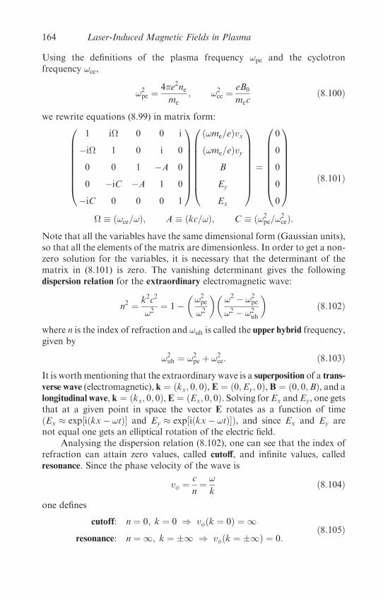
Using the definitions of the plasma frequency !pe and the cyclotronfrequency !ce,

!2pe ¼

4�e2neme

; !2ce ¼

eB0

mecð8:100Þ

we rewrite equations (8.99) in matrix form:

1 i� 0 0 i

�i� 1 0 i 0

0 0 1 �A 0

0 �iC �A 1 0

�iC 0 0 0 1

0BBBBBBBB@

1CCCCCCCCA

ð!me=eÞvxð!me=eÞvy

B

Ey

Ex

0BBBBBBBB@

1CCCCCCCCA

¼

0

0

0

0

0

0BBBBBBBB@

1CCCCCCCCA ð8:101Þ

� � ð!ce=!Þ; A � ðkc=!Þ; C � ð!2pe=!

2ceÞ:

Note that all the variables have the same dimensional form (Gaussian units),so that all the elements of the matrix are dimensionless. In order to get a non-zero solution for the variables, it is necessary that the determinant of thematrix in (8.101) is zero. The vanishing determinant gives the followingdispersion relation for the extraordinary electromagnetic wave:

n2 ¼ k2c2

!2¼ 1�

�!2pe

!2

��!2 � !2

pe

!2 � !2uh

�ð8:102Þ

where n is the index of refraction and !uh is called the upper hybrid frequency,given by

!2uh ¼ !2

pe þ !2ce: ð8:103Þ

It is worth mentioning that the extraordinary wave is a superposition of a trans-verse wave (electromagnetic), k ¼ ðkx; 0; 0Þ, E ¼ ð0;Ey; 0Þ, B ¼ ð0; 0;BÞ, and alongitudinal wave, k ¼ ðkx; 0; 0Þ,E ¼ ðEx; 0; 0Þ. Solving forEx andEy, one getsthat at a given point in space the vector E rotates as a function of timeðEx � exp½iðkx� !tÞ� and Ey � exp½iðkx� !tÞ�Þ, and since Ex and Ey arenot equal one gets an elliptical rotation of the electric field.

Analysing the dispersion relation (8.102), one can see that the index ofrefraction can attain zero values, called cutoff, and infinite values, calledresonance. Since the phase velocity of the wave is

v� ¼ c

n¼ !

kð8:104Þ

one defines

cutoff: n ¼ 0; k ¼ 0 ) v�ðk ¼ 0Þ ¼ 1

resonance: n ¼ 1; k ¼ 1 ) v�ðk ¼ 1Þ ¼ 0:ð8:105Þ


From the dispersion relation, equation (8.102), the resonances for the X-mode(the extraordinary wave) are at

X-mode resonances : ! ¼ 0; ! ¼ !uh ð8:106Þand the cutoffs are the solution of the following quadratic equation:

!4 � ð!2pe þ !2

uhÞ!2 þ !4pe ¼ 0: ð8:107Þ

Denoting the two solutions of this quadratic equation by !L and !R, andusing (8.103), one gets

! ¼ !ce

2þ

ffiffiffiffiffiffiffiffiffiffiffiffiffiffiffiffiffiffiffiffiffi!2pe þ 1

4!2ce

q; !þ � !R; !� � !L: ð8:108Þ

The notations R and L are used because these solutions describe right- andleft-handed circular polarization. The right-hand rotation of the electricfield is defined by the ‘right-hand rule’. If the thumb is along k then thefingers of the right hand are in the direction of the rotation of the electricfield for the R-wave. In the L-wave, E rotates in the opposite direction.

A schematic presentation of the dispersion relation ! ¼ !ðkÞ for extra-ordinary (X-mode) and ordinary (O-mode) waves, according to equations(8.102) and (8.97) respectively, is given in figure 8.4.

8.4.2 Electromagnetic waves propagating parallel to B0

In this case the following geometry is considered in Cartesian coordinates:

B0 ¼ ð0; 0;B0Þ; k ¼ ð0; 0; kÞ; E ¼ ðEx;Ey; 0Þ

B ¼ ðBx;By; 0Þ; v ¼ ðvx; vy; 0Þð8:109Þ

Figure 8.4. A schematic presentation of the dispersion relation ! ¼ !ðkÞ for extraordinary(X-mode) and ordinary (O-mode) waves.


Linearization and Fourier transform of equations (8.95) yields

ik� E� i!

cB ¼ 0

ik� Bþ i!

cEþ 4�ene

cv ¼ 0

�i!mevþ eEþ e

cv� B0 ¼ 0:

ð8:110Þ

Writing this equation explicitly, for the configuration defined in (8.109), inmatrix form we obtain

1 i� 0 0 i 0

i� 1 0 0 0 i

0 0 1 0 0 A

0 0 0 1 �A 0

�iK 0 0 �A 1 0

0 �iK A 0 0 1

0BBBBBBBBBBB@

1CCCCCCCCCCCA

ðme!=eÞvxðme!=eÞvy

Bx

By

Ex

Ey

0BBBBBBBBBBB@

1CCCCCCCCCCCA

¼

0

0

0

0

0

0

0BBBBBBBBBBB@

1CCCCCCCCCCCA

ð8:111Þ

� � !ce

!; A � kc

!; K �

!2pe

!2:

The dispersion relations are obtained by setting the determinant of thismatrix equal to zero:

n2 ¼ k2c2

!2

¼ 1�!2pe=!

2

1� !ce=!ð8:112Þ

whereþ and� denote right (R) and left (L) circular polarization, and nþ andn� are the indices of refraction for R and L waves propagating parallel to B0

respectively. See equations (8.53) and (8.54).From this dispersion relation we see that there is one resonance at

! ¼ !ce, and this is satisfied only for the R-wave. The cutoffs are derivedby equating k to zero in (8.112), implying the same results as those of theX-mode in equation (8.108).

Figure 8.5 shows the schematic dispersion relation ! ¼ !ðkÞ of anelectromagnetic wave propagating parallel to B0 for two cases: (a)!L < !pe < !ce, (b) !pe > !L > !ce. As can be seen from these figures,there are two R-mode branches (as in the X-mode, figure 8.4) but onlyone L-mode, where ! > !L is satisfied. The low-frequency branch of theR-wave is also known as the electron–cyclotron wave.

The dispersion relation (8.112) shows that the index of refraction for theright-hand and left-hand polarization are not equal, as already derived insection 8.3 (equations (8.53) and (8.54)). Moreover, the index of refractionis complex (i.e. n2 < 0; !2 < 0) in the domain !ce < ! < !R for the R-wave


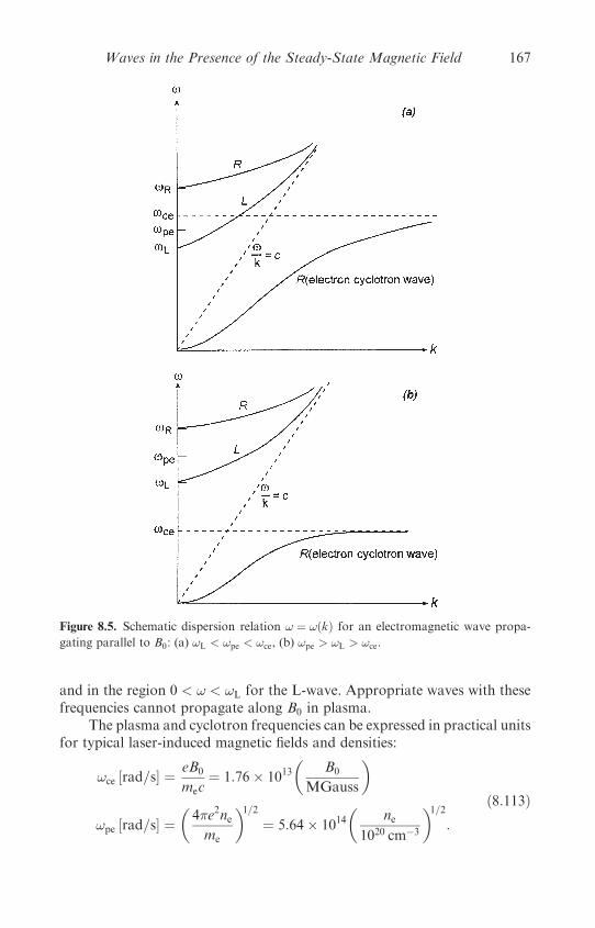
and in the region 0 < ! < !L for the L-wave. Appropriate waves with thesefrequencies cannot propagate along B0 in plasma.

The plasma and cyclotron frequencies can be expressed in practical unitsfor typical laser-induced magnetic fields and densities:

!ce ½rad=s� ¼eB0

mec¼ 1:76� 1013

�B0

MGauss

�

!pe ½rad=s� ¼�4�e2neme

�1=2¼ 5:64� 1014

�ne

1020 cm�3

�1=2:

ð8:113Þ

Figure 8.5. Schematic dispersion relation ! ¼ !ðkÞ for an electromagnetic wave propa-

gating parallel to B0: (a) !L < !pe < !ce, (b) !pe > !L > !ce.


Therefore, for figure 8.5(a) to be relevant for laser–plasma interactions, onerequires

!ce > !pe )�

B0

MGauss

�> 32:0

�ne

1020 cm�3

�1=2ð8:114Þ

while for figure 8.5(b) it is necessary that the opposite inequality is satisfied,which in general is more realistic for laser–plasma interactions.

Last but not least, from figure 8.5 at high frequencies (for typical laserintensities and B0, one usually has ! > !ce), one can see that the phasevelocity !=k is larger for an R-wave than for an L-wave. If a plane wave(i.e. linearly polarized) is propagating along B0, then this wave can bedescribed as a linear combination of an R-wave and an L-wave. Thesewaves (R and L) propagate with different phase velocity; therefore, theplane of polarization of the wave rotates as it travels along B0. This is theFaraday effect, as explained in section 8.3.

8.4.3 Alfven waves

So far, in this section, the ion motion was ignored. Now we combine the ionmotion with the electromagnetic equations (Maxwell equations). If an elec-tromagnetic wave propagates along the d.c. magnetic field, i.e. the wavevector k is parallel to the magnetic field in the plasma B0, one gets thefamous Alfven waves.

The following configuration is considered in Cartesian coordinates:

k ¼ ð0; 0; kÞ; B0 ¼ ð0; 0;B0Þ; E ¼ ðE; 0; 0Þ

B ¼ ð0;B; 0Þ; ve ¼ ðvex; vey; 0Þ; vi ¼ ðvix; viy; 0Þð8:115Þ

where ve and vi are the electron and ion velocities, and E and B are the elec-tromagnetic fields propagating in the plasma. It is assumed that the plasma isneutral and cold (Z is the ion charge):

ne ¼ Zni ¼ n0; Te ¼ Ti ¼ 0 ð8:116Þ

where ne and ni are the electron and ion densities, and T are appropriatetemperatures. Moreover, it is assumed that the electron inertia can beneglected in the momentum equation. In this case the relevant linearizedFourier transform fluid equations, together with Maxwell’s equations, are

0 ¼ �eE� ðe=cÞve � B0

�i!mivi ¼ ZeEþ ðZe=cÞvie � B0

ik� E ¼ ði!=cÞB

ik� B ¼ �ði!=cÞEþ ð4�=cÞn0ðvi � veÞ

ð8:117Þ


wheremi is the ion mass. Using similar algebra as before, one gets from theseequations the Alfven dispersion relation

!2 ¼ k2v2A1þ ðv2A=c2Þ

vA ¼�

B20

4�n0mi

�1=2� 2:18� 107

�mp

mi

��B0

MGauss

��1020 cm�3

ni

�1=2 � cms

�

ð8:118Þ

where vA is the Alfven wave velocity and mp is the proton mass. In derivingthis dispersion relation one must also assume that ! < !ci, where the ioncyclotron frequency is given by

!ci ¼ZeB0

mic� 9:58� 109

�Zmp

mi

��B0

MGauss

�: ð8:119Þ

The condition ! < !ci is nonrealistic for typical laser–plasma interactions.Moreover, using equation (8.118), one gets a time scale (�2�=!) largerby many orders of magnitude than any high-power laser pulse duration.Therefore, it seems that the Alfven waves do not play any important rolein laser–plasma interactions.

8.5 Resonance Absorption in a Magnetized Plasma

Resonance absorption was considered in section 5.6. In this section we analysehow the absorption is modified due to the presence of a steady-state (d.c.)magnetic field. As in the previous section, we consider the electron momentumequation together with Maxwell equations for cold plasma. In this case one isinterested in the effects of the density gradient, where the electric and magneticfields in the plasma can be written for a monochromatic wave:


Therefore, one cannot use the relation r ! ik when taking the Fouriertransform of the linear equations. However, the substitution @=@t ! �i!is permitted for the class of solutions given by (8.120). The linearized equa-tions to be solved are

r� EðrÞ ¼ i!

cBðrÞ

r � BðrÞ ¼ � i!

cEðrÞ � 4�ene

cv

�i!v ¼ � e

me

�EðrÞ þ 1

cv� B0ðrÞ

�ð8:121Þ

Resonance Absorption in a Magnetized Plasma 169

where v is the average velocity of the electrons, and the d.c. magnetic field istaken parallel to the z axis but is not necessarily a constant in space. The thirdof these equations can be written in matrix form as

vx

vy

vz

0B@

1CA ¼

�i!� !ce� 0

!ce� �i!� 0

0 0 �i=!

0B@

1CA

ðe=meÞEx

ðe=meÞEy

ðe=meÞEz

0B@

1CA

� � 1

!2 � !2ce

ð8:122Þ

where the electron cyclotron frequency is defined in (8.100). Substituting v

from (8.122) into the second equation of (8.121), one gets

r� BðrÞ ¼ � i!

ce � EðrÞ ð8:123Þ

where this equation defines the dielectric tensor e, given by

e ¼

!2 � !2uh

!2 � !2ce

i!2pe

ð!2 � !2ceÞ

0

�i!2pe!ce

!ð!2 � !2ceÞ

!2 � !2uh

!2 � !2ce

0

0 0 1�!2pe

!2

0BBBBBBB@

1CCCCCCCA

ð8:124Þ

where the plasma frequency is given in (8.100) and the upper hybridfrequency !uh is defined in (8.103). Note that the elements of the dielectrictensor are dimensionless.

In order to get the electromagnetic field, one has to solve equation(8.123) and the first equation of (8.121). The equation for the electricfield E is derived by taking r�[first equation of (8.121)] and using (8.123),yielding

r2EðrÞ þ !2

c2e � EðrÞ ¼ 0 ð8:125Þ

where the tensor e is given in (8.124). In deriving this equation it was assumedthat r � E ¼ 0, i.e. the plasma is neutral.

For the equation of the magnetic field B(r) it is convenient to use theinverse matrix e�1 of the dielectric tensor e. The inverse matrix is defined by

e�1 � e ¼ e � e�1 ¼ 1 ð8:126Þwhere 1 is the unit matrix

1 ¼1 0 0

0 1 0

0 0 1

0@

1A: ð8:127Þ


Using the tensor e�1, equation (8.123) can be rewritten by

e�1 � r � B ¼ � i!

cE: ð8:128Þ

Using equations (8.124) and (8.126), one gets the inverse tensor of e (Davidand Pellat 1980):

e�1 ¼"�1e �i 0

i "�1e 0

0 0 "�10

0BB@

1CCA

"e ¼��

1�!2pe

!2

�2� !2

ce

!2

��1� !2

uh

!2

��1

"0 ¼�1�

!2pe

!2

�2

¼!2pe!ce

!3

��1�

!2pe

!2

�2� !2

ce

!2

��1

:

ð8:129Þ

One can define "0 and "e as the square of the ordinary and extraordinaryindex of refraction respectively (see previous section).

The wave equation for the magnetic field B is derived by takingr� (8.128) and using the first equation of (8.121), together with theMaxwellequation r � B ¼ 0, implying

r� ðe�1 � r � BÞ � !2

c2B ¼ 0: ð8:130Þ

For the extraordinary mode the electric field E is perpendicular to the d.c.magnetic field B0. Choosing B0 to be in the z direction, the plane of the laserincidence is x–y, then the following configuration is defined (a p-polarization):

B0 ¼ ð0; 0;B0Þ; k ¼ ðk cos ; k sin ; 0Þ

E ¼ ðEx;Ey; 0Þ; B ¼ ð0; 0;BzÞ:ð8:131Þ

In this configuration the equation for Bz (the extraordinary mode) is derivedfrom equation (8.130):

r2Bz þ��r"e

"eþ i"ec

�� rBz þ k2"eBz ¼ 0; c � xx

@

@y� yy

@

@x:

ð8:132ÞFor an ordinary wave the electric field E is parallel to the d.c. magnetic fieldB0 (chosen in the z direction) and equation (8.125) in this case is

r2Ez þ k2"0Ez ¼ 0: ð8:133Þ


The ordinary wave, i.e. the s-polarization wave in our case, is not modified byan external magnetic field B0zz, and this wave does not drive the resonanceabsorption mechanism.

The p-polarization wave described above describes an extraordinary waveand can drive the resonance absorption mechanism (see section 5.5). It isconvenient to describe this case by the equation of the magnetic field (equation(8.132)). From this equation one gets a resonance for Bz, due to "e ¼ 0, at

resonance: !2 ¼ !2uh: ð8:134Þ

This resonance is responsible for the excitation of an electrostatic wave that is theorigin of the resonant absorption phenomenon. Two other singularities of equa-tion (8.132), where "e is zero and becomes infinite, are derived from solving

1�!2pe

!2¼ !ce

!: ð8:135Þ

However, Bz is regular at these points and these two singularities describe theturning points of the WKB solution (see section 5.4).

It is assumed that the laser is incident at x ¼ �L, in the x–y plane with apositive x component (the domain x < �L is vacuum and x > �L is plasma),and that the incident p-polarized wave is obliquely incident at an angle 0with the density gradient. For a constant (in space and time) externalmagnetic field and a linear density profile, described by

nenec

¼0 for x < �L

1þ ðx=LÞ for x > �L

� ) "0 ¼

1 for x < �L

�ðx=LÞ for x > �L

�

ð8:136Þequation (8.132) takes the form (David and Pellat 1980)

d2B

d�2þ�1

�� 1

� � �� 1

� þ �

�dB

d�

þ��2

�� 2 þ �

� � ��

� þ �

�B ¼ 0: ð8:137Þ

The following change of variables is used in equation (8.132) in order to getequation (8.137):

Bz ¼ BðxÞ expðiky sin 0Þ

� ¼ x

�k2

L

�1=3

� ¼ ðkLÞ1=3 sin 0

� ¼ ðkLÞ2=3�!ce

!

�:

ð8:138Þ


Moreover, equation (8.137) is derived only for !ce=!� 1 (i.e. we neglectð!ce=!Þ2 and higher-order terms), an assumption satisfied in most laser–plasma experiments.

As we have seen in chapter 5, without a dissipation mechanism such aselectron ion–collisions or Landau damping, all of the laser light is reflected(or transferred, if the plasma density is smaller than the critical densityeverywhere) out of the plasma (i.e. no absorption). In order to obtain alaser absorption one requires an effective collision frequency �eff. If themechanism of the damping of electrostatic waves is known then it is possibleto include � implicitly in the dielectric constant, e.g. changing equation(8.136) to

"0 ¼1 for x < �l

�ðx=LÞ þ ið�eff=!Þ for x > �L:

�ð8:139Þ

However, it turns out that in most cases the collision frequency determinesthe magnetic (or electric) field strength at resonance and its spatial structurethere, but does not modify the qualitative values of the absorption coefficient.The amplitude ratio square between the outgoing and incoming wave (atx ¼ �L in our above example) gives the reflection coefficient R (1� R isthe absorption coefficient). This value does not depend on �eff as long as itis not zero. In this case equation (8.137) is solved numerically by integrating

Figure 8.6. Absorption of p-polarized laser at oblique incidence in magnetized plasma. �

and � are defined in equation (8.138). The dots are experimental points (Horovitz et al.

1998) of � and �. The measured absorption at these points fits within 10% of the theoretical

values given in this figure.


it along a path in the complex plane (of �), where the singularities are avoidedby taking a ‘detour’ from the x axis (i.e. the real � axis). The solution for thelaser absorption, as given in figure 8.6 (Woo et al. 1978, David and Pellat1980), shows that a p-polarized laser at oblique incidence in magnetizedplasma can be almost 100% absorbed.

It turns out that the laser absorption depends only on two parameters, �and �, defined in equation (8.138). � is related to the density gradient (scalingas L) and to the incidence angle 0, while � is related both to the densitygradient and the magnetic field. It is interesting to point out that even atnormal incidence (0 ¼ 0), the absorption can be as high as 50% for� � 0:5. Using practical units for laser–plasma interactions, one can write

� � 0:148

��L1 mm

��L

10 mm

�2�1=3� B0

MGauss

�ð8:140Þ

so that � � 0:5 for a magnetic field �3MG and a density scale length�10 mm, values measured experimentally in many plasmas created by lasers.


Chapter 9

Thermal Conduction and Heat Waves

9.1 The Scenario

Thermal conduction or, in more general terms, the energy transport in laser-produced plasma, is related to basic plasma physics in a wide range ofparameters, such as density and temperature. This subject is of great interestbecause it plays a very important role in major applications, such as inertialconfinement fusion (ICF), the production of x-ray sources and x-ray lasers.For example, the acceleration of shell targets for ICF relies not only on theenergy absorbed by the plasma, but also on the efficient coupling betweenthis energy and the solid shell. In section 9.2 we calculate this efficiency ina simple model.

A high intensity laser radiation (>1011 W/cm2), with pulse duration �Llarger than 100 ps, is incident on a solid target. Plasma is created instanta-neously (on a time scale shorter than �L by many orders of magnitude); itis heated to a high temperature and this plasma expands into the vacuumto create a low-density corona. Once the plasma corona is created, thelaser radiation no longer reaches the solid since it cannot penetrate beyondthe critical surface, with an electron density nec ¼ 1021(�L=mm)�2 cm�3,where �L is the laser wavelength. At the critical surface, part of the laserbeam is absorbed and the other part is reflected into the corona. We haveseen in chapter 5 that most of the absorption is done in the domain nearthe critical surface. Moreover, as has been shown in chapter 6, waves arecreated in the plasma-corona.

Figure 9.1 describes schematically the temperature and the electrondensity in laser-produced plasma. The temperature has a maximum in theregion of the critical surface, where most of the laser energy is absorbed.The temperature decreases sharply towards the cold solid, and to a goodapproximation it is constant throughout the corona. The density isdecreasing towards the vacuum and, for laser radiation intensities largerthan about 1015 W/cm2, there is a steep density gradient at the critical

175

surface. The density and pressure rise towards the solid surface and thepressure (ablation pressure) reaches a maximum at the ablation surface,where plasma is created and the flow velocity is zero.

The energy absorbed at the critical surface domain is transportedbeyond the critical surface towards the solid target, either by (x-ray)radiation or by electron thermal conduction (figure 9.1). Most of theelectrons in the plasma have a Maxwellian velocity distribution, with atemperature usually denoted by Tc (c stands for ‘cold’, which can be ofthe order of kBTc � 1 keV). For high laser intensities IL, satisfying

Figure 9.1. Schematic diagram of the temperature and density profile in a laser-induced

plasma. A scenario is given for plasma particle streams, currents, heat flow, laser and

laser-induced x-ray propagation, a possible double layer formation and the creation of

axial and toroidal magnetic fields.

176 Thermal Conduction and Heat Waves

IL�2L > 1014 (W=cm2)mm2, the electron velocity distribution may be described

by two (or more) Maxwellian distributions with a second temperature Th,much larger than Tc. In this case the fast electrons with a temperature Th,which are created in the critical surface domain, transport part of theirenergy into the solid, causing preheating of the target. This is easily understoodsince the electron mean free path �e (for 908 deflection in multiple Coulombcollisions with ions, see section 9.3) is proportional to the square electrontemperature,

�eðcmÞ ¼ 5:71� 104T2e

Zne ln�ð9:1Þ

where Te, in degrees Kelvin, stands for the electron (cold or hot) temperature,Z is the charge of the ion, ne is the electron density and ln� is the Coulomblogarithmic factor. For example, for Te ¼ 107 K � 1 keV, Z ¼ 10, ln� ¼ 10and ne ¼ 1020 cm�3, one gets �e � 5:7 mm. When Th=Tc � 10, the energy ofthe hot electrons is deposited 100 times deeper into the target than theenergy deposited by the cold electrons. Furthermore, if the cold electronmean free path is smaller than the temperature density gradient, thenthe thermal conduction is diffusive (see section 9.4) and the heat flux q

(erg/(s�cm2)) is given by (see section 2.3)

q ¼ � 13�evenekBrTe ¼ �rTe ð9:2Þ

where ve is the electron velocity and kB is Boltzmann’s constant. Substituting(9.1) into (9.2), one gets the classical result of Spitzer and Harm, denoted bySH theory (see section 9.5) for the conductivity �:

�ðerg � s�1 � cm�1 �K�1Þ ¼ 1:77� 10�6 T5=2e

Z ln�: ð9:3Þ

The heat flow is possible due to the distortion of the Maxwellian velocitydistribution. For example, in one dimension the Gaussian form of theelectron velocity distribution is changed in such a way that more electronshave a suitable velocity and energy to carry heat to the cold region. Thiseffect creates an electric field E. In order to keep charge neutrality, an electriccurrent �EE (�E is the electrical conductivity coefficient), called ‘returncurrent’, is created from the cold target towards the critical surface (seefigure 9.1). The electrons in the return current have low energy. The thermalflux of electrons, from the critical surface towards the ablation surface, hasa higher energy than the electrons in the return current, so the target isheated.

The temperature gradient between the critical surface and the ablationsurface induces a thermoelectric effect. This phenomenon reduces the classical

The Scenario 177

heat flow according to the relation

J ¼ �EE� �rT ; q ¼ �E� �rT ð9:4Þ

where J is the total electrical current, and the coefficients �, �, �E and �are not independent (Onsager relations in irreversible thermodynamics).Assuming only a net heat flow transport, J ¼ 0, one gets from (9.4):

q ¼ ��1� ��

�E�

�rTe ð9:5Þ

where a reduction factor due to the thermoelectric effect shows up, whichmay reduce the heat transport by a factor of about 2.

Furthermore, the heat transport of the cold electrons for very steeptemperature gradients does not satisfy the diffusion approach. The SHtheory is valid only if the electron velocity distribution function f isslightly perturbed from its equilibrium distribution ( f0 is the Maxwelldistribution), namely f ¼ f0 þ f1 where f0 � f1. The validity of the diffusionapproximation (SH model) depends strongly on the ratio �e=LT, where �e isthe electron mean free path (see (9.1)) and LT is the temperature densityscale length:

LT ¼ T

ðdT=dxÞ : ð9:6Þ

The diffusion approximation is valid for �e � LT. It has been shown (Grayand Kilkenny 1980) that the diffusion approximation is valid only for�e=LT < 10�2. For �e=LT > 10�2 the energy transport is significantlyreduced, and it is necessary to introduce an inhibition factor f in order toget agreement with experiments. The inhibition factor f is defined as theratio between the actual heating flux q and the free streaming flux qf, themaximum possible flux, defined by

qf ¼ nekBTe

�kBTe

me

�1=2: ð9:7Þ

The free streaming is the heat flow carried by the electrons if they streamfreely at their thermal velocity along the temperature gradient. For highlaser irradiance, IL > 1015 W/cm2, where �e=LT � 1, the agreement withexperiments are obtained when using an electron thermal flux

q ¼ f qf � 0:03qf ð9:8Þ

instead of the diffusion flux given by (9.2) (see, for example, Rosen 1984).As we have seen in chapter 8, magnetic fields of the order of few

megagauss are easily created in the corona of laser-produced plasma (see


figure 9.1). Magnetic fields significantly affect the electron transport if

!ce�e > 1; !ce ¼eB

mecð9:9Þ

where �e is the angular scattering time of the electron and !ce is the Larmorangular frequency. Assuming that the main contribution to �e is fromelectron–ion collisions, then (see section 2.2)

�e½s� � �ei ¼ 3:44� 10�16

��10

Z

��1022 cm�3

ne

��10

ln�

��Te

100 eV

�3=2�ð9:10Þ

and using

!ce½s�1� ¼ 1:76� 1013�

B

MGauss

�ð9:11Þ

one gets in practical units

!ce�e ¼ 6:05� 10�3

�10

Z

��1022 cm�3

ne

��10

ln�

��Te

100 eV

�3=2� B

MGauss

�:

ð9:12Þ

The megagauss magnetic fields were measured in the corona, where theelectron density is much smaller than 1022 cm�3 and the temperature canbe much larger than 100 eV. In this case !ce�e can be larger than one, andtherefore in the corona the electron transport in a magnetized plasmamight be relevant. However, in the more important domain of the energytransport, between the critical surface and the ablation surface, !ce�e is ingeneral smaller than one even if the large magnetic field penetrates fromthe corona into the solid. Thus the electron transport between the criticalsurface and the ablation surface seems not to be affected significantly bythe magnetic field. We shall not further discuss in this chapter the transportin magnetized plasma.

Electron transport also plays an important role in spreading theabsorbed laser energy uniformly around the solid target. It is well knownthat a high-laser-intensity beam does not have a uniform spatial distribution,and even for the same laser system the spatial intensity distributionchanges from shot to shot. Therefore, a major difficulty in high-intensitylaser–plasma experiments is the non-uniformity of the laser beams. Thiscan cause irreproducible and uncontrollable experiments, and therefore isdifficult to analyse and use in various applications (such as ICF). However,after a corona with a dimension much larger than the laser wavelength hasbeen formed, the energy transport in the lateral direction (in the plasma)can redistribute the energy uniformly around the solid surface. Electron

The Scenario 179

conduction reduces the temperature within ‘hot spots’ and thus decreases thepossible creation of hot and narrow filaments in the plasma.

Regarding the scenario in the corona, it is interesting to point out thepossible existence of a double layer (DL) (see figure 9.1). The creation ofhot electrons, also known as suprathermal electrons (see section 9.6), with atemperature higher by a factor of 10 or more than the cold temperature (thethermal electrons) may be associated with the formation of this DL in theexpanding corona. The fastest particles, electrons and ions, in the low-densityregion lead the expansion of the plasma. The electric field in the expanding DLaccelerates the ions and causes the fast electrons to turn back into the target.Such DLs were observed experimentally (Eliezer and Ludmirsky 1983) andsuggested theoretically by the prediction of ‘rarefaction shock waves’ forTh=Tc > 9:9 (Bezzerides et al. 1978, Wickens et al. 1978, Diebold et al.1987). A rarefaction shock occurs (Zeldovich and Raizer 1966) when thefollowing unusual condition is satisfied: d2P=dV2 < 0, V ¼ 1=�, � ¼ mini ina plasma and P is the pressure. In this case P is composed of two components:P ¼ nckBTh þ nhkBTh, where nh and nc are the electron densities of the hotand cold plasmas respectively.

Electron transport in plasmas has been a major issue since the beginningof modern plasma physics (Spitzer and Harm 1953, Rosenbluth et al. 1957,Spitzer 1962, Braginskii 1965, Trubnikov 1965, Hinton and Hezeltine 1976,Stacey 1980, Nicholson 1983, Horton 1989, Hazeltine and Meiss 1992). Theelectron transport phenomena in laser-produced plasma have been exten-sively discussed in the literature (Haines 1980, 1989, Key 1980, 1983, 1991,Bobin 1985, Shvarts 1986, Galeev and Natanzon 1991, Yamanaka 1991,Bell 1995). In this chapter we discuss electron transport phenomena relevantto laser-produced plasma.

9.2 The Rocket Model

We now consider a planar steady-state ablation from a target, as shownschematically in figure 9.1. In this section it is assumed that the fluxes ofmass, momentum and energy are constant and the equation of state of anideal gas is used:

flux of mass ¼ �u

flux of momentum ¼ Pþ �u2

flux of energy ¼ �

��1Puþ 1

2�u3 þ qþ I

ð9:13Þ

where u is the plasma flow velocity, � is the density, P is the pressure, q is theelectron heat flux, I is the absorbed laser energy flux (erg s�1 cm�2) and � isthe ratio of the heat capacity at constant pressure (CP) to heat capacity at


constant volume CV. The following ideal gas equations of state are alsoavailable:

internal energy: " ¼ CVT ¼�

1

� � 1

�P

�

enthalpy: h ¼ CPT ¼�

�

� � 1

�P

�

� ¼ CP

CV

¼ gþ 2

g

isothermal (T ¼ const:Þ speed sound: cT ¼ffiffiffiffiP

�

s

isentropic (S ¼ const:Þ speed sound: cS ¼ffiffiffiffiffiffi�P

�

s

ð9:14Þ

where g is the number of degrees of freedom of one particle. For a mono-atomic gas g ¼ 3 and � ¼ 5

3. For electrons in the plasma � ¼ 53, so that

�=ð� � 1Þ ¼ 52.

We now write six equations describing the flux conservation for mass,momentum and energy, according to (9.13), at the critical surface and atthe ablation surface:

at the critical surface:

�cuc ¼ �u � _mm

�cu2c þ Pc ¼ �u2 þ P

_mm

��5

2

�Pc

�cþ�1

2

�u2c

�þ qout ¼ _mm

��5

2

�P

�þ�1

2

�u2�þ qin þ I

qout ¼ �u3c ¼ _mmu2c ðfree streaming plasmaÞ

ð9:15Þ

at the ablation surface:

_mm ¼ �u ¼ const: ð‘source’ of plasmaÞ

Pa ¼ �u2 þ P ðablation pressureÞ

_mm

��5

2

�P

�þ�1

2

�u2�þ qin ¼ 0

where the quantities with the index c denote the variables at the criticalsurface from the corona side, while those without the index c denote thevalues between the corona and the ablation surface. Note that at the ablationsurface u ¼ 0 and P ¼ Pa. Since in the corona the temperature is constant toa good approximation, it is conceivable that the plasma expands with the

The Rocket Model 181

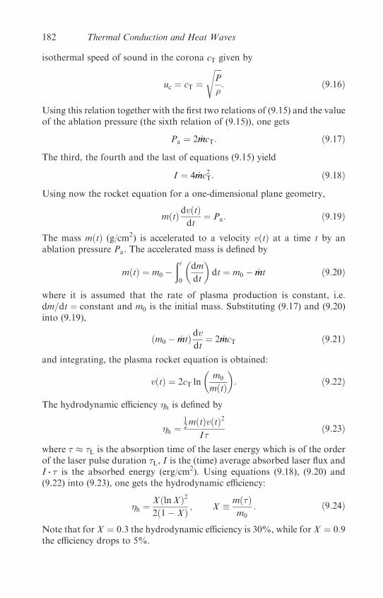
isothermal speed of sound in the corona cT given by

uc ¼ cT ¼ffiffiffiffiP

�

s: ð9:16Þ

Using this relation together with the first two relations of (9.15) and the valueof the ablation pressure (the sixth relation of (9.15)), one gets

Pa ¼ 2 _mmcT: ð9:17Þ

The third, the fourth and the last of equations (9.15) yield

I ¼ 4 _mmc2T: ð9:18Þ

Using now the rocket equation for a one-dimensional plane geometry,

mðtÞ dvðtÞdt

¼ Pa: ð9:19Þ

The mass mðtÞ (g/cm2) is accelerated to a velocity vðtÞ at a time t by anablation pressure Pa. The accelerated mass is defined by

mðtÞ ¼ m0 �ðt0

�dm

dt

�dt ¼ m0 � _mmt ð9:20Þ

where it is assumed that the rate of plasma production is constant, i.e.dm=dt ¼ constant and m0 is the initial mass. Substituting (9.17) and (9.20)into (9.19),

ðm0 � _mmtÞ dvdt

¼ 2 _mmcT ð9:21Þ

and integrating, the plasma rocket equation is obtained:

vðtÞ ¼ 2cT ln

�m0

mðtÞ

�: ð9:22Þ

The hydrodynamic efficiency h is defined by

h ¼12mðtÞvðtÞ2

I�ð9:23Þ

where � � �L is the absorption time of the laser energy which is of the orderof the laser pulse duration �L, I is the (time) average absorbed laser flux andI � � is the absorbed energy (erg/cm2). Using equations (9.18), (9.20) and(9.22) into (9.23), one gets the hydrodynamic efficiency:

h ¼ XðlnXÞ2

2ð1� XÞ ; X � mð�Þm0

: ð9:24Þ

Note that for X ¼ 0:3 the hydrodynamic efficiency is 30%, while for X ¼ 0:9the efficiency drops to 5%.


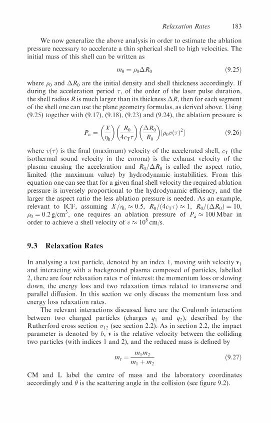
We now generalize the above analysis in order to estimate the ablationpressure necessary to accelerate a thin spherical shell to high velocities. Theinitial mass of this shell can be written as

m0 ¼ �0�R0 ð9:25Þ

where �0 and �R0 are the initial density and shell thickness accordingly. Ifduring the acceleration period � , of the order of the laser pulse duration,the shell radius R is much larger than its thickness�R, then for each segmentof the shell one can use the plane geometry formulas, as derived above. Using(9.25) together with (9.17), (9.18), (9.23) and (9.24), the ablation pressure is

Pa ¼�X

h

��R0

4cT�

��R0

R0

�½�0vð�Þ2� ð9:26Þ

where vð�Þ is the final (maximum) velocity of the accelerated shell, cT (theisothermal sound velocity in the corona) is the exhaust velocity of theplasma causing the acceleration and R0=�R0 is called the aspect ratio,limited (the maximum value) by hydrodynamic instabilities. From thisequation one can see that for a given final shell velocity the required ablationpressure is inversely proportional to the hydrodynamic efficiency, and thelarger the aspect ratio the less ablation pressure is needed. As an example,relevant to ICF, assuming X=h � 0:5, R0=ð4cT�Þ � 1, R0=ð�R0Þ ¼ 10,�0 ¼ 0:2 g/cm3, one requires an ablation pressure of Pa � 100Mbar inorder to achieve a shell velocity of v � 108 cm/s.

9.3 Relaxation Rates

In analysing a test particle, denoted by an index 1, moving with velocity v1and interacting with a background plasma composed of particles, labelled2, there are four relaxation rates � of interest: the momentum loss or slowingdown, the energy loss and two relaxation times related to transverse andparallel diffusion. In this section we only discuss the momentum loss andenergy loss relaxation rates.

The relevant interactions discussed here are the Coulomb interactionbetween two charged particles (charges q1 and q2), described by theRutherford cross section �12 (see section 2.2). As in section 2.2, the impactparameter is denoted by b, v is the relative velocity between the collidingtwo particles (with indices 1 and 2), and the reduced mass is defined by

mr ¼m1m2

m1 þm2

ð9:27Þ

CM and L label the centre of mass and the laboratory coordinatesaccordingly and is the scattering angle in the collision (see figure 9.2).

Relaxation Rates 183

Conservation of momentum and energy of the Coulomb collision yieldsthe scattering angle in the centre of mass (CM) system (in c.g.s. units):

tan

�CM2

�¼ jq1q2j

mrv2b

ð9:28Þ

and the scattering angle of particle 1 in the laboratory frame is given by

cot L ¼ cot CM þm1

m2

�1

sin CM

�: ð9:29Þ

Figure 9.2. (a) Laboratory and (b) centre of mass (CM) frames of reference. In (a) the orbit

is shown for a charged particle with mass m1 scattered by a charged particle (with opposite

charge) with mass m2, positioned at O.


Since the collisions of interest are between the pairs electron–electron (ee),electron–ion (ei), ion–electron (ie) and ion–ion (ii), the following specialcases are of interest:

m1 � m2: L � CM

m1 ¼ m2: L � CM2

m1 � m2: L � m2

m1

sin CM:

ð9:30Þ

All particles of type 1 incident into a ring between b and bþ db are scatteredinto angles CM and CM þ dCM in the CM frame of reference (or into anglesL and L þ dL in the laboratory frame of reference). Therefore, the impactparameter b is related to the differential cross section d�12 by

d�12ðCMÞ ¼ �12ðCMÞ d� ¼ �12ðCMÞ2� sin CM dCM ¼ 2�b db ð9:31Þ

where � is the solid angle and �ðCMÞ is the Rutherford cross section (using(9.28)):

�ðCMÞ ¼ b db

sin CM dCM¼

ðq1q2Þ2

½2mrv2 sin2ðCM=2Þ�2

: ð9:32Þ

Since the angle of deflection increases with the decrease of the impact para-meter (see (9.28)), the cross section that a particle is scattered at any anglelarger than 908 is given by the impact parameter for ¼ 908:

�12ðCM 908Þ ¼ �bð908Þ2 ¼ �q21q22

m2rv

4ð9:33Þ

where equation (9.28) has been used.Equation (9.33) gives the cross section for a scattering angle larger than

or equal to 908 in one collision. Now we calculate small-angle scattering thatadds up to a large angle, say 908 deflection. We denote the small-anglescattering in the centre of mass frame by ð� 1Þ. From equation (9.28),

¼ 2jq1q2jmrv

2b: ð9:34Þ

The mean square deflection of a particle (called the test particle) that goesalong a distance L in a plasma with a density of particles n2 (here we calculatethe deflection caused by particles of type 2) is

2CM ¼X

2 ¼ n2L

ðmax

min

2�12ðÞ2� sin d

¼ 18�n2Lq21q

22

m2rv

4

ðbmax

bmin

db

b¼ 18�n2Lq

21q

22 ln�

m2rv

4ð9:35Þ


where the Coulomb cutoff coefficient is defined by the ratio of Debye lengthto the distance of closest approach (see section 2.2):

� ¼ bmax

bmin

¼�

3

2ffiffiffi�

p��

1

q1q22

��ðkBTÞ3

n2

�1=2: ð9:36Þ

The following relation has been used between the relative velocity v and thetemperature T :

12mrv

2 ¼ 32 kBT : ð9:37Þ

The mean free path for large angle deflection, L90, is obtained from (9.35) bysubstituting there 2CM ¼ 1, yielding the cross section �90 for a large-anglescattering due to many small-angle deflections,

L90 ¼m2

rv4

18�q21q22n2 ln�

¼ ðkBTÞ2

2�q21q22n2 ln�

�90 ¼1

n2L90

¼ 18�q21q22 ln�

m2rv

4¼ 2�q21q

22 ln�

ðkBTÞ2

ð9:38Þ

where (9.37) has been used. Note that the first of equations (9.38) is the equa-tion given in (9.1) (q1 ¼ �e, q2 ¼ Z and Zn2 ¼ ne).

It is important to note that the probability (which is proportional to thecross section) of a large-angle scattering due to a single collision (in mostplasmas) is significantly smaller than the probability of a large deflectioncaused by many small-angle scatterings:

�90�ðCM 908Þ ¼ 8 ln�: ð9:39Þ

Equation (9.39) is derived from equations (9.33) and (9.38). The factor of8 ln� is in the domain of 10–102 for most plasma systems discussed in thisbook. This fact is very important in analysing collision phenomena inplasmas.

The time required for large-angle deflection, in the CM system, isobtained from (9.38) and (9.37):

�90 ¼L90

v¼

�3

ffiffiffi3

p

8�

� ffiffiffiffiffiffimr

p ðkBTÞ3=2

q21q22n2 ln�

: ð9:40Þ

We are interested in the large-angle deflection times in the laboratory frameof reference. Therefore, from equation (9.30), one gets that if m2 m1 thenthe deflection in the laboratory system is comparable with that in the CMsystem, so that the calculated value of L90 in the CM system is the same


as in the laboratory system. Therefore, one can use the above formulaefor e–e, e–i and i–i collisions. However, for i–e collisions (the test particleis the ion which is scattered by electrons) it follows from equation (9.30)that L ðme=miÞCM, i.e. since me=mi is about 1/2000 (for the hydrogenplasma) the test particle (the ion) must travel a 2000 times larger distancein order to undergo a large deflection in the laboratory frame. Forthe identical particle collisions the reduced mass is half the particlemass, and a factor of 2 was introduced since L � 1

2 CM (see equation(9.30)).

From the above formalism (equation (9.40)) the following collisiontimes for large-angle scattering, or equivalently themomentum loss relaxation

times � , are obtained (we drop the subscript 90), as seen in the laboratoryframe of reference (note that the first particle in the superscript is the test

particle):

�ee ¼�3

ffiffiffi6

p

8

� ffiffiffiffiffiffime

p ðkBTÞ3=2

�e4ne ln�

� 1:07� 10�11

�1020 cm�3

ne

��10

ln�

��Te

1 keV

�3=2½s�

� ii ¼�3

ffiffiffi6

p

8

� ffiffiffiffiffimi

p ðkBTÞ3=2

�Z4e4ni ln�

� ei ¼�3

ffiffiffi3

p

8

� ffiffiffiffiffiffime

p ðkBTÞ3=2

�Z4e4ni ln�

� ie ��mi

me

��ei:

ð9:41Þ

Assuming a neutral plasma, ne ¼ Zni and the same temperature, one canget from the last equation the following order of the large-angle deflectioncollision times:

�ee : � ei : � ii : � ie � 1 :1

Zffiffiffi2

p :1

Z3

�mi

me

�1=2:

1

Z3ffiffiffi2

p�mi

me

�: ð9:42Þ

The large-angle scattering collision time calculated here is an approximationof the momentum loss of the test particle. If a particle has an initial momen-tum in some direction, after scattering to a large angle the momentum in theinitial direction is lost.

We now estimate the time required for a test particle to lose itsenergy. From momentum and energy conservation during a collision, atest particle 1, with energy E1, is releasing energy �E1 in the laboratory


frame according to the equation

�E1

E1

¼ 4m1m2

ðm1 þm2Þ2sin2

�CM2

�: ð9:43Þ

The energy lost in multiple-scattering small-angle collisions can be calculatedby substituting CM ¼ 908 in the last equation, yielding

�E1

E1

¼ 2m1m2

ðm1 þm2Þ2: ð9:44Þ

Therefore, in 908 collisions between identical particles, half of the initialenergy is transferred by the test particle to the background particles.However, for electron–ion scattering only the fraction me=mi of the initialenergy of the test particle is transferred during 908 deflection. Denoting by�E the energy relaxation time, i.e. the time that �E1=E1 � 1, one gets fromequations (9.41), (9.42) and (9.44) (for ne ¼ Zni),

�eeE � � ee

� iiE � � ii � 1

Z3

�mi

me

�1=2� ee

� eiE � 1

Z

�mi

me

��ee

� ieE ��mi

me

�� ie �

�mi

me

�2�ei

�ee : � eeE : � iiE : � eiE � 1 : 1 :1

Z3

�mi

me

�1=2:1

Z

�mi

me

�:

ð9:45Þ

To conclude this analysis, it is important to note that the collision frequency�12 for momentum loss and the collision frequency �12E for the energy loss,where 1 denotes the test particle and 2 the background particles, are relatedto the relaxation times calculated above by

�12 ¼ 1

�12; �12E ¼ 1

�12E: ð9:46Þ

The last of equations (9.45) show that electrons equilibrate, i.e. reach anequilibrium distribution (e.g. a Maxwell distribution of velocities), on ashorter time scale than the ions do by a factor of Z3ðme=miÞ1=2. Moreover,the electrons reach equilibrium with the ions on a time scale longer by afactor ð1=ZÞðmi=meÞ than the electrons equilibrate with themselves. Forexample, in a typical corona of laser-produced plasma with an electrondensity 1020 cm�3, an ion charge Z ¼ 10, mi=me � 4� 104 and an electrontemperature 1 keV, ln� � 10, one gets from equations (9.41) and (9.45)


that we can define an electron temperature after 10 ps from the start of thelaser–target interaction, an ion temperature after 2 ps (note that for ahydrogen plasma this relaxation time changes to 200 ps) and that the elec-tron temperature is equal to the ion temperature after 40 ns. Thus, for mosthigh-intensity laser pulses (0.1 ns to 10 ns) there is no equilibrium between theelectrons and the ions in the corona. It is worth mentioning that for a solidstate density plasma, ne � 1023, produced for example by a very short pulseduration (100 fs), the above time scales are reduced by a factor of 1000(assuming the same temperature). In this case the electrons will reach anequilibrium distribution with a temperature of 1 keV in about 10 fs.

The multiple small-angle scattering of the plasma introduces theCoulomb logarithm ln�, a factor included in the transport coefficients aswell. ln� ¼ bmax=bmin results from integration over the scattering angles ,between large angles resulting from a small impact parameter bmin andsmall angles resulting from a large impact parameter bmax. The value ofbmax is taken as the Debye shielding scale and is a function of electronvelocity (i.e. temperature) and density. If the electrons move in a strongmagnetic field, where the Larmor radius is smaller than the Debye length,then the Larmor radius should replace the value of bmax. However, this isseldom required in the laser-produced plasma. Last but not least, in denseand cold plasma the values of bmax and bmin are comparable and ln� maybecome negative, an unphysical result. This can happen when a large-angledeflection is more probable than the small-angle scattering. Such a plasmamedium is the strongly-coupled plasma, where the electric potential energyis larger than the kinetic energy. In this case a value of ln� ¼ 2 is takenfor practical calculations.

In conclusion, for plasmas where the small-angle scatterings are domi-nant, the Coulomb scattering of the plasma particles has a randomizingeffect on the particle motion. Therefore, in this case, the electron driftmotion may be described by diffusion or in the more general case by theFokker–Planck equation.

9.4 The Fokker–Planck Equation

The electron energy transport can be described by the Boltzmann equation(see section 3.4):

@f

@tþ v � @f

@rþ eE

me

� @f@v

¼�@f

@t

�coll

ð9:47Þ

where f ¼ f ðr; v; tÞ is the electron density in phase space, r� v space, r is thespace coordinate and v is the particle velocity. E is the electrical field in theplasma and the magnetic field is neglected in (9.47). ð@f =@tÞcoll is the collisionterm describing the scattering of electrons (by electrons and ions), as

The Fokker–Planck Equation 189

described in the previous section. Assuming that the small-angle collisionsare dominant, one can use the Fokker–Planck equation for the collisionterm.

The Fokker–Planck equation is derived in general by assuming aMarkov process. If a measurable physical quantity develops in time in sucha way that its ‘future value’ depends only on its ‘present value’, then thephenomenon describing this physical quantity is called a Markov process.In such a process the physical quantity changes in a random way. Let ustake a physical variable X with measured values Xn, Xn�1, . . . , X1, X0 attimes tn > tn�1 > � � � > t1 > t0 respectively. The probability P to measurethe value Xn, where the previous values were Xn�1, . . . , X1, X0, in aMarkov process is given by

PðXnjXn�1; . . . ;X1;X0Þ ¼ PðXnjXn�1Þ: ð9:48Þ

This equation describes the fact that the value Xn, measured at time tn,depends only on its value Xn�1 as measured at time tn�1. A trivial examplefor a Markov process is the flipping of a coin. Then the number Xn of headsafter n flips depends only on the number of heads Xn�1 after n� 1 flips, andnot on all the history.

In analysing a continuous Markov process the situation is more com-plicated. If the physical phenomenon is described by a continuous function,then the existence of the derivatives contradicts the definition of the Markovprocess. For example, in this case Xnþ1 depends not only on Xn but alsoon the derivative ðdXn=dtÞ ¼ ðXn � Xn�1Þ=�t, etc. Therefore, a Markovprocess may describe a continuous physical phenomenon only as an approx-imation. For example, in a Brownian motion the particle velocity undergoesa rapid variation due to each molecular collision, followed by a low-ratechange due to the friction force. On a time scale of one collision the scatteringis not Markovian. However, on a time scale of many collisions the Markovprocess is a very good approximation.

In plasma, due to the long-range Coulomb forces there are manysmall-angle scatterings causing large deflections (see previous section). Thedistribution function f ðv; tÞ is changing slowly on a time scale t describingone (small-angle) collision. The Markov process may describe the changeson a time scale �t, due to many small-angle collisions. In this case it isrequired that t � �t; however, �t is small enough to define the variationsand the derivatives of the physical quantities.

According to equation (9.48) for a Markov process the distributionfunction f ðv; tÞ is determined from the knowledge of f ðv� w; tÞ, wherew ¼ �v is the change in velocity in the time interval �t due to multiplesmall-angle collisions. It is assumed here that the distribution function inphase-space can be written f ðr; v; tÞ ¼ n0 f ðv; tÞ, where the spatial depen-dence is given by the constant n0 (dimension cm�3). The probability that aparticle changes its velocity from v to vþ w is given by Pðv;wÞ. If only


collisions are responsible to the change in f ðv; tÞ, then one can write

f ðv; tÞ ¼ðPðv� w;wÞf ðv� w; t��tÞ d3w

� f ðv; tÞðPðv;wÞ d3w��t

@f ðv; tÞ@t

ðPðv;wÞ d3w

�ðX

i

wi

@

@vi½Pðv;wÞf ðv; tÞ�d3w

þ 1

2

ðXi; j

wiwj

@2

@vi @vj½Pðv;wÞ f ðv; tÞ� ð9:49Þ

where a Taylor expansion has been made to second order, a good approxi-mation for w small and�t small. The indices i and j are the vector componentsin an orthogonal frame of reference. The integral of the probability functionis one: ð

Pðv;wÞ d3w ¼ 1 ð9:50Þ

and the rate of change of the first moment hwi (dimension cm/s2) and thesecond moments hwwi (dimension cm2/s3) of w are

hwii ¼1

�t

ðPðv;wÞwi d

3w

hwiwji ¼1

�t

ðPðv;wÞwiwj d

3w:

ð9:51Þ

Substituting (9.50) and (9.51) into (9.49), one gets the Fokker–Planck

equation�@f

@t

�coll

¼ �Xi

@

@vi½hwiif ðv; tÞ� þ

1

2

Xi; j

@2

@vi @vj½hwiwjif ðv; tÞ�: ð9:52Þ

The first term on the right-hand side describes a ‘drift’, while the second termis the diffusion in the velocity space. In uniform plasma in thermal equili-brium the drift term ‘pushes’ the electrons to a zero velocity, but the electronsdo not accumulate there because the diffusion term ‘pushes’ them away fromthe zero velocity.

The Fokker–Planck equation (9.52) can also be viewed as a continuityequation in the velocity space, with a density f ðvÞ and a current JðvÞ:�

@f

@t

�coll

þ @

@v� Jv ¼ 0; Jv ¼ hwif � 1

2

@

@v� ½hwwif �: ð9:53Þ

As in the previous section, the test particles are denoted by index 1 andthe background particles acquire index 2. The probability per unit time


(P d3v=�t) in equations (9.51) that a test particle, moving with relativevelocity v1 � v2 relative to a background particle (moving with velocity v2),is scattered by the background particles, with a density f2 d

3v, into thesolid angle d� is given by

Pðv1; v2Þ d3v2�t

¼ f2ðr2; v2; tÞ�12ðv;�Þvd3v2 d�; v � jv1 � v2j ð9:54Þ

where �12 is the Rutherford cross section given in the CM frame by (9.32).The approximation f ðr; v; tÞ ¼ nðrÞf ðv; tÞ is used, where nðrÞ is the spatialdensity. nðrÞ is omitted in the following analysis, since it cancels out in theFokker–Planck equation (9.52). Note that the dimension of f ðr; v; tÞ is(cm�6 s3), while the dimension of f ðv; tÞ is (cm�3 s3).

Substituting (9.54) into (9.51), one has to calculate the averages

hw1i ¼ðd3v2

ðd�w1v�ðv;�Þf2ðv2Þ

hw1w1i ¼ðd3v2

ðd�w1w1v�ðv;�Þf2ðv2Þ

w1 ¼ v01 � v1ðin lab: frameÞ ¼ m2

m1 þm2

ðv0 � vÞ � m2

m1 þm2

w ð9:55Þ

v ¼ v1 � v2

v0 ¼ v

01 � v

02

�ðin CM frameÞ

v ¼ jvj ¼ jv0j

where primes denote the velocity value after the collision. The third equationof (9.55) is derived from the relation between the particle velocity in thelaboratory frame and the particle velocity in the CM frame:

v1ðlabÞ ¼ vcm þ�

m2

m1 þm2

�v

v01ðlabÞ ¼ vcm þ

�m2

m1 þm2

�v0

v2ðlabÞ ¼ vcm ��

m1

m1 þm2

�v

v02ðlabÞ ¼ vcm �

�m1

m1 þm2

�v0

ð9:56Þ

where vcm is the velocity of the centre of mass. The last equation of (9.55)is obtained by using in the centre of mass energy conservation ð 12m1v

21 þ

12m2v

22 ¼ 1

2m1v021 þ 1

2m2v022 Þ and momentum conservation (m1v1 þm2v2 ¼ 0;

m1v01 þm2v

02 ¼ 0).


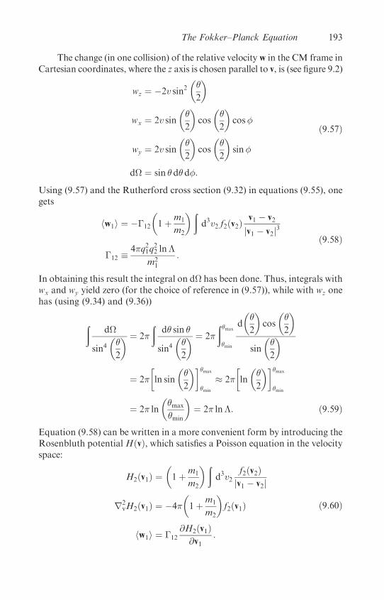
The change (in one collision) of the relative velocity w in the CM frame inCartesian coordinates, where the z axis is chosen parallel to v, is (see figure 9.2)

wz ¼ �2v sin2�

2

�

wx ¼ 2v sin

�

2

�cos

�

2

�cos�

wy ¼ 2v sin

�

2

�cos

�

2

�sin�

d� ¼ sin d d�:

ð9:57Þ

Using (9.57) and the Rutherford cross section (9.32) in equations (9.55), onegets

hw1i ¼ ��12

�1þm1

m2

�ðd3v2 f2ðv2Þ

v1 � v2

jv1 � v2j3

�12 �4�q21q

22 ln�

m21

:

ð9:58Þ

In obtaining this result the integral on d� has been done. Thus, integrals withwx and wy yield zero (for the choice of reference in (9.57)), while with wz onehas (using (9.34) and (9.36))

ðd�

sin4�

2

� ¼ 2�

ðd sin

sin4�

2

� ¼ 2�

ðmax

min

d

�

2

�cos

�

2

�

sin

�

2

�

¼ 2�

�ln sin

�

2

��max

min

� 2�

�ln

�

2

��max

min

¼ 2� ln

�max

min

�¼ 2� ln�: ð9:59Þ

Equation (9.58) can be written in a more convenient form by introducing theRosenbluth potential HðvÞ, which satisfies a Poisson equation in the velocityspace:

H2ðv1Þ ¼�1þm1

m2

�ðd3v2

f2ðv2Þjv1 � v2j

r2vH2ðv1Þ ¼ �4�

�1þm1

m2

�f2ðv1Þ

hw1i ¼ �12

@H2ðv1Þ@v1

:

ð9:60Þ


Using the differentiation laws,

@2jv1 � v2j@v1i @v1j

¼ @

@v1i

�v1j

jv1 � v2j

�¼

ijjv1 � v2j

�v1iv1j

jv1 � v2j3ð9:61Þ

and neglecting the integral terms not containing d= (considered to besmall), one gets (i and j are the three components of an orthogonal frameof reference)

G2ðv1Þ ¼ðd3v2 f ðv2Þjv1 � v2j

r4VG2ðv1Þ ¼ �8�f2ðv1Þ

hw1iw1ji ¼ �12

@2G2

@v1i @v2j:

ð9:62Þ

Substituting (9.60) and (9.62) into (9.52), one gets the Fokker–Planckequation

�@f�ðr; v; tÞ

@t

�coll

¼X�

��

��X3i¼1

@

@vi

�f�ðv; tÞ

@H�

@vi

�

þ 1

2

X3i; j¼1

@2

@vi @vj

�f�ðv; tÞ

@2G�

@vi @vj

��ð9:63Þ

where f� is the distribution of the �-th species of particles and the sum � onthe right-hand side of (9.63) is over the collisions with the backgroundparticles (for the test particle �). The Rosenbluth potentials in (9.63) aredefined according to (9.60) and (9.62):

H�ðvÞ ¼�1þm�

m�

�ðd3u

f�ðuÞjv� uj ; G�ðvÞ ¼

ðd3ujv� uj f�ðuÞ ð9:64Þ

and the coupling constants �� are given in the approximation of equation(9.58) by

�� ¼ 4�q21q22n� ln�

m2�

: ð9:65Þ

The density of the � particles n� has been included in (9.65) (in comparisonwith (9.58)) since the left-hand side of (9.63) describes the full distribution inphase space. This is necessary in order to substitute (9.63) (together with(9.64) and (9.65)) into the Boltzmann equation (9.47). The Boltzmannequation with the collisional term given in (9.63) is occasionally called theFokker–Planck equation.


9.5 The Spitzer–Harm Conductivity

Knowledge of the time development of a fully ionized plasma due to collisionsrequires the simultaneous solution of the collisions of electrons with electrons,electrons with ions, ions with electrons and ions with ions. The general solutionof these nonlinear integral-differential equations is not an easy task and can bedone only with large computer resources. It is therefore very useful to look forsimpler but approximate solutions that enable us to generate simple modelsof transport. The analytical models are very useful to comprehend thecomplicated phenomena of heat transfer in laser–plasma interaction.

For a distribution function depending on one space–one velocitycoordinates x and v, and on the angle between the velocity and the spatialcoordinate, f ¼ f ðx; v; cos ; tÞ, the Fokker–Planck equation (9.63) can alsobe written as (Shkarofsky et al. 1966)�

@f

@t

�coll

¼ 1

v

@

@v

�v2�Djj2

@f

@vþ Cf

��þ D?2v2 sin

@

@

�sin

@f

@

�ð9:66Þ

where C (dimension (s�1)), Djj (dimension (cm s�2)) and D? (dimension(cm2 s�3)) are the coefficients of slowing down, diffusion in velocity spaceand diffusion in angular space respectively. These coefficients depend onthe distribution function of the plasma electrons and ions. The angulardiffusion term is dominated by electron–ion collisions, while the velocitydiffusion term and the slowing down are more affected by electron–electroncollisions. Therefore, for plasma with ion charge Z, the second term on theright-hand side of equation (9.66) is about Z times larger than the firstterm on the right-hand side of this equation (see equation (9.42), where thecollision frequencies are proportional as ��1

ee :��1ei ¼ 1 :Z).

If a plasma has a temperature gradient scale LT much larger than theelectron mean free path �e, �e � LT (�e and LT are defined in (9.1) and(9.6)) and the distribution function has a weak angular dependence, thenthe electron distribution function can be expressed by the first two terms ina cos perturbation expansion

f ðx; v; ; tÞ ¼ f0ðx; v; tÞ þ f1ðx; v; tÞ cos ð9:67Þ

where f0 and f1 are the isotropic and the anisotropic components respectively.Since the large electron–ion collision frequency tends to maintain thedistribution function almost isotropically, it is possible to neglect thehigher-order terms in cos in the expansion (9.67).

The isotropic component is assumed to be equal to the equilibriumMaxwellian distribution fM:

f0 ¼ fM ¼ ne

ð�Þ3=2v3Texp

�� v2

v2T

�; f 1 � fM; vT �

ffiffiffiffiffiffiffiffiffiffiffiffi2kBT

me

s: ð9:68Þ

The Spitzer–Harm Conductivity 195

The Boltzmann equation with the Fokker–Planck collision term has ananalytic solution for the Lorenz plasma, i.e. ions with large Z, where f1, theelectric field E, @fM=@x and @fM=@t are small quantities (i.e. second-orderterms or higher are neglected). Moreover, it is assumed that @fM=@t ¼ 0and @f1=@t ¼ 0. In the Fokker–Planck equation (9.66) only the secondterm on the right-hand side contributes to a Lorenz plasma. Therefore,within those approximations, the Boltzmann equation (9.47) simplifies to

v@fM@x

þ eE

me

@fM@v

¼ � A

v3f1

A � vD? ¼ 8�Znee4 ln�

me

¼ v3T�ei

¼ v4T�e

ð9:69Þ

where �ei is given in equation (9.41) and the electron mean free path �e equalsL90 (for e–i collisions) in equation (9.40).

An additional equation is needed for the electric field E. Assumingcharge neutrality in the plasma, which means that there is no electric currentalong the density gradient, gives the equation

J ¼ 4�e

3

ð10f1v

3 dv ¼ 0: ð9:70Þ

This model, the Lorentz model, is described mathematically by equations(9.68), (9.69) and (9.70). Substituting (9.68) into (9.69) and using

1

ne

@ne@x

¼ 1

Ln

;1

T

@T

@x¼ 1

LT

ð9:71Þ

one gets

f1 ¼ � v3

A

�v

Ln

� 3v

2LT

þ v3

v2TLT

� 2eEv

mev2T

�fM: ð9:72Þ

Substituting f1 from (9.72) into (9.70) and usingð10

dv v2kþ1 exp

�� v2

2v2T

�¼ k!

2ð2v2TÞkþ1; k ¼ 0; 1; 2; 3; . . . ð9:73Þ

one gets an expression for the electric field (that cancels the current inducedby the temperature gradient, see (9.4)):

2eE

mev2T

¼ eE

kBT¼

�1

Ln

þ 5

2LT

�: ð9:74Þ

This electric field is inserted into (9.72) to give the anisotropic electrondistribution function f1:

f1 ¼ne

ð�Þ3=2ALTv3T

�4v4 � v6

v2T

�exp

�� v2

v2T

�: ð9:75Þ


The heat flow is calculated by integrating in the velocity space the driftingelectron distribution. The number (per cm3) of drifting electrons withvelocities between zero and v is given by 4

3�v3f1, and each electron carries

an energy 12mev

2. Therefore, the heat flux q is given by

q ¼ 2�me

3

ð10f1v

5 dv ¼ mene

3ð�Þ1=2ALTv3T

ð10

dv

�4v9 � v11

v2T

�exp

�� v2

v2T

�: ð9:76Þ

After integrating (9.76) the heat flux is

q ¼ ��

4ffiffiffi�

p�menev

7T

ALT

¼ ��12ffiffiffi�

p��evTnekB

dT

dxð9:77Þ

where A was taken from equation (9.69), the relation between vT and T isgiven in (9.68) and LT was substituted from (9.71). The heat flux in thisequation is the Lorentz limit of the Spitzer–Harm conductivity. The classicalSpitzer–Harm conductivity has been analytically derived in agreement, up toa constant, with the coefficient � in (9.2). Substituting the free-streaming fluxfrom (9.7) into the flux (9.77), one gets

q /��eLT

�qf ð9:78Þ

and for �e=LT � 1 this is a reasonable result.For �e=LT > 1 (even for �e=LT > 0:1 using the above numerical

coefficients) the diffusion flux q is becoming larger than the free-streamingflux, which is absurd. In typical high-power laser-produced plasmas, betweenthe critical surface and the ablation surface, the criterion �e=LT � 1 is notsatisfied. Therefore, the heat transport between the critical surface and theablation surface cannot be described by the diffusion approximation, or byapproximating the collision term in the Boltzmann equation by theFokker–Planck equation. Another approach is needed in laser–plasmainteractions in order to calculate how the energy is transported into thetarget. For this purpose the heat inhibition factor was introduced.

Another way to come to the same conclusion is to analyse f1=fM. Usingequations (9.75), (9.68) and (9.69), this ratio is

f1fM

¼��eLT

��v

vT

�4�4�

�v

vT

�2�: ð9:79Þ

This equation shows that f1=fM increases with �e=LT and is equal to one forsome value of the electron velocity v. However, the Spitzer–Harm approxi-mation is valid only for f1=fM � 1. Between the ablation surface and thecritical surface, LT is chosen positive (i.e. dT=dx > 0); therefore, the positivex axis is pointing towards the laser radiation source (i.e. towards the vacuum)(see figure 9.1). The differential heat flux qðvÞ, which is is proportional to

The Spitzer–Harm Conductivity 197

f1v5 (the integrand in (9.76)), is positive (flow towards the vacuum) if f1 > 0

and negative when f1 < 0. Since f1=fM < 0 for v > 2vT ( fM is alwayspositive), all electrons with a velocity higher than 2vT are transporting heatinside the target, while those electrons with v < 2vT are carrying energyfrom the ablation surface towards the corona. The reverse flow at lowvelocities is caused by the electric field and it is referred to in the literatureas the ‘return current’. The return current carries an equal but opposite currentto that transported by the high-velocity electrons heating the target. Thisphenomenon ensures quasi-neutrality. The total heat flow is negative (see(9.77)); therefore, a net energy is transported into the target, so that the heatis predominantly carried by electrons with velocities between 2vT and 3vT.

The total distribution function (9.67) can be written

f ¼ fM þ f1 cos ¼ fM

�1þ

�f1fM

�vxv

�: ð9:80Þ

For particles moving into the target, vx=v ¼ 1, and therefore f becomesnegative (an impossible situation) at f1=fM < �1. Analysing equation(9.79), one gets the unphysical situation, negative f , even for apparently alarge temperature scale length such as LT=�e ¼ 150 if v=vT � 2:65, a non-negligible region of energy transport into the target. It turns out thatLT=�e > 103 is required for the Spitzer–Harm approximation to be valid.Between the corona and the ablation surface this constraint is not usuallysatisfied. The steep temperature gradient in laser-produced plasmas requires,in general, a different formalism in order to explain the energy transport.

If there is a steep temperature gradient the electrons which have a longmean free path modify the local distribution function. This phenomenon iscalled non-local transport, since a large domain affects the heat transport.Because of the difficult problems of heat transport, between the coronaand the ablation surface, a phenomenological approach is taken by usingan effective inhibition factor in front of the free-streaming flow of electrons(see equation (9.8)).

In the next section a short discussion is given on the existence of hot elec-trons. In this case the physical phenomena are explained by two temperatures(or more), which in turn are derived from two (or more) Maxwellian electrondistribution functions.

9.6 Hot Electrons

In laser-produced plasma the energy is absorbed by the electrons. When theseelectrons collide with the ions they are decelerated and emit x-ray radiationdue to the bremsstrahlung effect. The logarithm of the energy spectrum of anx-ray when plotted as a function of the photon energy is a straight line if theelectron distribution is Maxwellian. From the slope of this line the electron


temperature is deduced. This phenomenon is explained in the followingparagraphs.

If there are two species of electrons then attempts are made todescribe the electrons by two temperatures. Two temperatures imply twoMaxwellian electron distributions, and the logarithm of the energy spectrumof x-ray when plotted as a function of the photon energy is described by a‘broken line’. From the slopes of the two lines the two temperatures can bededuced. It has been found experimentally that at laser intensities largerthan 1015 W/cm2, the x-ray emission from the laser-irradiated targets havean energy spectrum induced by a double Maxwellian electron distribution(Haines 1980).

The acceleration aðtÞ of an electron while colliding with an ion, withcharge Ze at a distance r, is given by the Coulomb force (c.g.s. units):

aðtÞ ¼ Ze2

merðtÞ2: ð9:81Þ

Classical electrodynamics shows that the accelerated electron radiates apower P:

PðtÞ ¼ 2e2a2

3c3¼

�2Z2e6

3m2ec

3

�1

r4ð9:82Þ

where c is the speed of light and equation (9.81) has been used. Integratingover r and multiplying by the density numbers of the electron and the iongives the total density power Qb (erg/cm3 s), emitted by bremsstrahlung:

Qb ¼2Z2e6neni3c3m2

e

ð1rmin

4�r2 dr

r4¼ 8�Z2e6neni

3c3m2ermin

: ð9:83Þ

At rmin the classical approximation is no longer valid, since the uncertaintyprinciple does not permit localization of the electron to a zero volume. Asoccasionally done in plasma physics, one takes the de Broglie scale lengthfor rmin and relates the electron velocity to the temperature

rmin ¼ �h

mev; v ¼

ffiffiffiffiffiffiffiffiffikBT

me

s: ð9:84Þ

Substituting (9.84) into (9.83), the total power emitted per unit volume by theelectrons, due to bremsstrahlung, is

Qb ¼�16�2Z2e6nenik

1=2B

3c3hm3=2e

�T

1=2e : ð9:85Þ

In order to measure the electron temperature, a knowledge of the photonenergy spectrum is required, rather than the total density power given in

Hot Electrons 199

this equation. For this purpose we analyse the energy " emitted by oneelectron during the time it interacts with one ion. Equation (9.82) yields

" ¼ðþ1

�1P dt ¼ 2e2

3c3

ðþ1

�1aðtÞ2 dt �

ð10P� d� ð9:86Þ

where P� is the radiated energy per unit frequency emitted (by one electronpassing an ion) with a frequency �. In classical mechanics the electrontrajectory and its acceleration are calculated for the electron passingan ion, assuming that the energy loss of the electron is neglected (this approx-imation is correct for weak radiation). In a Coulomb interaction between twocharges q1 and q2 with a reduced mass mr, the trajectory rðtÞ and theacceleration aðtÞ are conveniently given as a function of a parameter �, theimpact parameter b and the relative velocity v (see figure 9.2(a)):

t ¼ 1

2

��þ �3

3

��m2

rb3v3

q21q22

�; r ¼ 1

2ð1þ �2Þ

�mrb

2v2

jq1q2j

�

cos’ � � 1� �2

1þ �2; sin’ � 2�

1þ �2

a? ¼ d2

dt2ðr sin’Þ ¼

�q1q2mrbv

2

�3�v2b

�8�

ð1þ �2Þ3

ajj ¼d2

dt2ðr cos’Þ ¼ �

�q1q2mrbv

2

�3�v2b

�4ð1� �2Þð1þ �2Þ3

a2 ¼ a2? þ a2jj:

ð9:87Þ

The solution aðtÞ is substituted into (9.86) so that " is calculated exactly(Miyamoto 1980). Here an estimate is given (Zeldovich and Raizer 1966,Haines 1980), which is correct within a constant of about 2, and the exactsolution is quoted at the end of this calculation.

The time of interaction between the electron and the ion is of theorder � � b=v. The dominant frequency in the Fourier transport is2�� 1=� � v=b (the dominant Fourier transport frequency usually satisfies!� � 1, where ! ¼ 2��). Therefore, we can use these relations and (9.81) toobtain

� ¼ v

2�b; d� ¼ � v db

2�b2ð9:88Þ

" ¼�2e2a2

3c3

�� ¼

�2Z2e6

3c3m2e

�1

b3v: ð9:89Þ

The electron with energy " undergoes ni�ðbÞv collisions per unit time withions in the impact parameter range b to bþ db, where the cross section is


�eiðbÞ ¼ 2�b db. Therefore, the energy radiated per unit time by an electron is

dE

dt¼

ð1bmin

"niv2�b db ¼ 4�Z2e6ni3m2

ec3

ð1bmin

db

b2¼ 8�2Z2e6ni

3m2ec

3v

ð�max

0d�

dE

dt¼

ð�max

0q� d�

q� �8�2Z2e6ni3m2

ec3v

h�max ¼ 12mev

2

ð9:90Þ

where (9.88) is used and the photon energy (h�) cannot be larger than thekinetic energy of the electron. The power radiated per unit volume by theelectrons is obtained by using (9.90):

Qb �ðd�Q� ¼

ðd�

ð1 ffiffiffiffiffiffiffiffiffiffiffi2h�=me

p q�ne fMðvÞ4�v2 dv

fMðvÞ ¼�

1

�v2T

�3=2exp

�� v2

v2T

�

v2T ¼ 2kBTe

me

Q� ¼�8

ffiffiffi2

p

3

��3=2Z2e6nine

m3=2e c3ðkBTeÞ1=2

exp

�� h�

kBTe

�:

ð9:91Þ

An exact calculation yields 4=ffiffiffi3

p� 2:3 times Q� of equation (9.91). The

integral of (9.91) gives (9.85).From equation (9.91) it is evident that a plot of ln½dQb=dðh�Þ� versus h�

yields a straight line, and from the slope it is easy to deduce the electrontemperature. If the electron velocity distribution can be described not byone Maxwellian (as in the proof of (9.91)), but as a superposition of twoMaxwellian distributions with two temperatures, then the integral of (9.91)yields

Q� /nc

T1=2c

exp

�� h�

kBTc

�þ nh

T1=2h

exp

�� h�

kBTh

�ð9:92Þ

where nc and nh are the spatial densities of the cold and hot electron species,while Tc and Th are their respective temperatures. Such a spectrum wasmeasured (Haines 1980) for neodymium laser pulses of the order of 1 nsand with intensity larger than 1015 W/cm2 (see figure 9.3).

Energy transfer from electron plasma waves, nonlinear wave phenomenaand resonance absorption can create the hot electrons. It appears that the

Hot Electrons 201

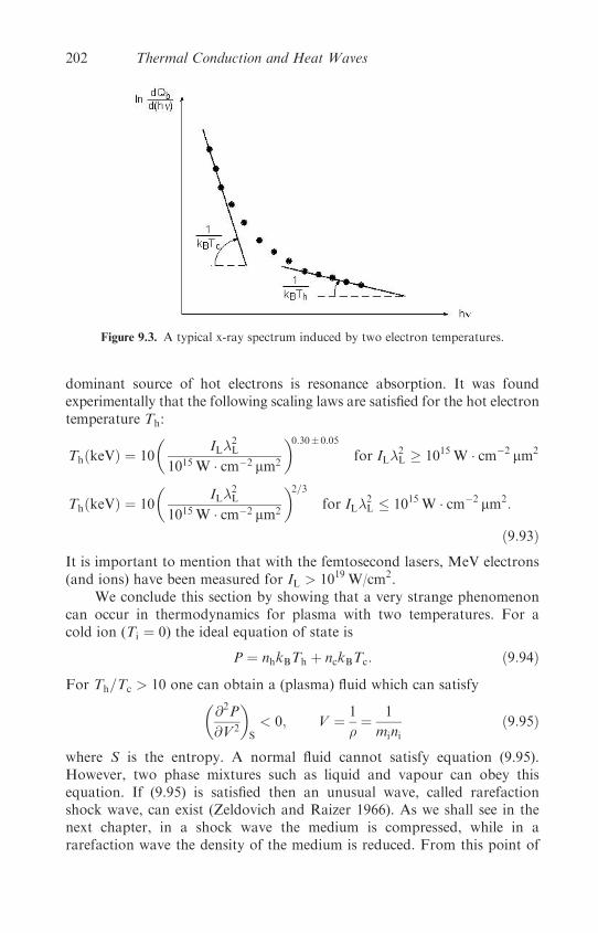
dominant source of hot electrons is resonance absorption. It was foundexperimentally that the following scaling laws are satisfied for the hot electrontemperature Th:

ThðkeVÞ ¼ 10

�IL�

2L

1015 W � cm�2 mm2

�0:30�0:05

for IL�2L 1015 W � cm�2 mm2

ThðkeVÞ ¼ 10

�IL�

2L

1015 W � cm�2 mm2

�2=3for IL�

2L � 1015 W � cm�2 mm2:

ð9:93ÞIt is important to mention that with the femtosecond lasers, MeV electrons(and ions) have been measured for IL > 1019 W/cm2.

We conclude this section by showing that a very strange phenomenoncan occur in thermodynamics for plasma with two temperatures. For acold ion (Ti ¼ 0) the ideal equation of state is

P ¼ nhkBTh þ nckBTc: ð9:94Þ

For Th=Tc > 10 one can obtain a (plasma) fluid which can satisfy�@2P

@V2

�S

< 0; V ¼ 1

�¼ 1

minið9:95Þ

where S is the entropy. A normal fluid cannot satisfy equation (9.95).However, two phase mixtures such as liquid and vapour can obey thisequation. If (9.95) is satisfied then an unusual wave, called rarefactionshock wave, can exist (Zeldovich and Raizer 1966). As we shall see in thenext chapter, in a shock wave the medium is compressed, while in ararefaction wave the density of the medium is reduced. From this point of

Figure 9.3. A typical x-ray spectrum induced by two electron temperatures.


view the rarefaction shock wave behaves like a rarefaction wave. However,while in a rarefaction wave the entropy S is conserved, in a shock wave theentropy increases, and in the rarefaction wave the entropy is decreasing: anunstable process.

In the following, we write the fluid equations for the plasma expandinginto vacuum, where the plasma has two components of electrons (Bezzerideset al. 1978, Wickens et al. 1978). The continuity and the momentumequation for the ions moving without collisions in the electrostatic potential� are

@ni@t

þ @

@xðniviÞ ¼ 0; mi

�@vi@t

þ vi@vi@x

�¼ �Ze

@�

@x: ð9:96Þ

Neglecting the inertial term in both electronic fluids, the pressure of the hotand cold electrons are balanced by the potential force

enc@�

@x� kBTc

@nc@x

¼ 0 ) nc ¼ nc0 exp

�e�

kBTc

�

enh@�

@x� kBTh

@nh@x

¼ 0 ) nh ¼ nh0 exp

�e�

kBTh

�:

ð9:97Þ

The temperatures Tc and Th are assumed constants. Equations (9.96) and(9.97) are solved, together with the requirement of charge neutrality:

Zni ¼ nc þ nh: ð9:98Þ

Using (9.94), (9.97) and (9.98), one can write the second equation of (9.96) inthe following ways:

@vi@t

þ vi@vi@x

¼ � 1

nimi

@P

@x¼ � 1

nimi

@P

@ni

@ni@x

¼ �cSð�Þ21

ni

@ni@x

cSð�Þ2 ¼1

mi

@P

@ni¼ 1

mi

@P

@�

�@ni@�

��1

¼ Z

mi

�nh þ nc

ðnh=kBThÞ þ ðnc=kBTcÞ

�:

ð9:99Þ

We now look for a self-similar solution, like the one obtained in section 7.2, inanalysing the plasma expansion into vacuum. The variables nc, nh, ni, vi and� are functions of only one variable �:

� ¼ x

t;

@

@x¼ 1

t

@

@�;

@

@t¼ � �

t

@

@�: ð9:100Þ

Using these relations in the two equations of (9.96), where the secondequation is taken from (9.99), one gets

�vi � � ni

c2s=ni vi � �

��dni=d�

dvi=d�

�¼

�0

0

�: ð9:101Þ

Hot Electrons 203

Equations (9.101) have a solution only if the determinant of the matrixvanishes, implying

vi ¼ csð�Þ þ �: ð9:102Þ

Substituting this relation into one of the equations of (9.101), one gets

nidvid�

þ csð�Þdnid�

¼ 0: ð9:103Þ

Using (9.97) and (9.98), with the boundary condition � ¼ 0, v ¼ 0 andcs ¼ c0 in the undisturbed plasma, one obtains after integrating (9.103) thefollowing solution:

vi ¼�

1

Tc

� 1

Th

��1� ccTc

ln

��cs � ccc0 � cc

��c0 þ cccs þ cc

��

þ chTh

ln

��ch � c0ch � cs

��ch þ csch þ c0

��

c2c �ZkBTc

mi

; c2h � ZkBTh

mi

c20 ¼�

Z

mikB

�nc0 þ nh0

ðnc0=TcÞ þ ðnh0=ThÞ:

ð9:104Þ

From (9.102) and (9.104) the solution of the potential �ð�Þ is obtained,implying for Th=Tc > 10 a jump in the potential as shown schematically infigure 9.1 (the double layer).

The jump in the potential and the rarefaction shock wave areobtained if

d2P

dV2¼ n3im

3i c

2s

�2þ dc2s

d�

�� 0: ð9:105Þ

Using (9.97) and (9.99) in this inequality, we get

2þ dc2sd�

� 0 ) 2�2 þ �ð6�� 1� �2Þ þ 2�2 � 0

� � Th

Tc

; � � nhnc:

ð9:106Þ

This equation has a real solution for � only if

ð6�� 1� �2Þ2 � 16�2 0 ) � � Th

T c

5þffiffiffiffiffi24

p� 9:9: ð9:107Þ


In this domain of parameters the function �ð�Þ is not well defined, i.e. � hasthree values for the same �, therefore the jump of � (the singularity) is settledin this domain and a rarefaction wave is obtained.

Hot electrons is a peculiar and interesting phenomenon associatedwith high-power laser-produced plasmas. Sometimes this phenomenon isdisturbing, like the preheating of solid targets for applications of shockwaves, and sometimes it is a desirable effect, like in the creation of sourcesof high-energy x-rays.

9.7 Heat Waves

The local absorption of the laser energy is associated with the creation of atemperature gradient and a thermal flux to transport the absorbed energy.With the temperature gradient there are also pressure gradients that set theplasma into a ‘fluid’ motion. In most laser-produced plasmas the hydro-dynamic energy transport substantially exceeds the heat conduction.However, in the interaction of very short laser pulses (of the order of 1 psor less) with matter, the hydrodynamic motion does not have time todevelop, and therefore in these cases the heat transport is dominant. Elec-trons or x-rays may serve as heat carriers (Ditmire et al. 1996, Fraenkelet al. 2000). For nonlinear transport coefficients, like the electron conduc-tivity discussed in section 9.5, we expect that the energy transport is causedby a heat wave. Heat waves may also play an important role in inertialconfinement fusion during the ignition process. In this section we shallformally show the solution for a one-dimensional geometry heat wave(Zeldovich and Raizer 1966, Krokhin 1971).

Let us consider the energy conservation equation:

�CV

@T

@t¼ �r � ðqH � IÞ; qH ¼ ��rT ; � ¼ BTn; r � I � W

ð9:108Þ

where � is the density (g/cm3), T is the temperature in Kelvin, I is theabsorbed laser flux [erg/(time � cm2)], qH is the heat flux [erg/(time � cm2)], �is the coefficient of thermal conductivity [erg/(cm � s �K)], W is the powerdensity deposited by the laser [erg/(s � cm3)],CV is the specific heat at constantvolume [erg/(g �K)], and B and n are constants. In one space dimension,chosen as x, and assuming a constant density � (a reasonable assumptionfor short laser pulse duration) and a constant CV, equation (9.108) takesthe form

@T

@t¼ @

@x

��@T

@x

�þ w; � ¼ �

�CV

; w ¼ W

�CV

: ð9:109Þ

Heat Waves 205

The coefficient� is called the thermal diffusivity (cm2/s) and can be expressed as

� ¼ aTn ð9:110Þ

where a is a constant.If n ¼ 0, i.e. a constant thermal diffusivity, then equation (9.109) is

the simple diffusion equation. Assuming that the laser energy is depositedat x ¼ 0 (e.g. all the energy is deposited at the critical surface located atx ¼ 0) and at time t ¼ 0 (i.e. a very short pulse duration), then

@T

@t¼ a

�@2T

@x2

�þ w; w ¼ T0L ðxÞ ðtÞ; Tðx; 0Þ ¼ T0L ðxÞ ð9:111Þ

where ðxÞ and ðtÞ are the Dirac delta functionðL=2�L=2

ðxÞ dx ¼ 1;

ð�=2��=2

ðtÞ dt ¼ 1 ð9:112Þ

and L is a scale length factor for the energy deposition and � is the laser pulseduration. The solution of equation (9.111) is

Tðx; tÞ ¼ T0L

ð4�atÞ1=2exp

�� x2

4at

�: ð9:113Þ

Equation (9.113) is the solution of the linear heat transport equation (9.111).The nonlinear heat transport equation is

@T

@t¼ a

@

@x

�Tn @T

@x

�þ w: ð9:114Þ

For example, for electrons in plasma one can use equation (9.2) (proven insection 2.3), together with the CV value of 3

2 kB per particle, to get

� ¼ 13�evenekB

CV ¼ 32 kB

�ne�

�9>=>; ) � ¼ �

�CV

¼ 2

9�eve / T5=2 ð9:115Þ

where we have used equation (9.1), the electron mean free path �e � T2, andthe thermal speed of the electron ve � T1=2. Therefore, for the nonlinearelectron heat transport in the plasma, n ¼ 5

2 in equation (9.114). In com-parison, for radiation (x-rays) transport in a multiply-ionized plasma thepower of T in this equation is in the domain 4.5–5.5.

In some cases, like in a solid medium, CV depends on temperature(CV=particle equals 3kB/2 only for an ideal gas with three degrees of free-dom). In this case equation (9.114) is not satisfied. When the specific heatis a function of the temperature, one can write for the energy E (erg/g),

E ¼ �Tk ) T ¼�E

�

�1=k

; CV ¼�@E

@T

�V

¼ �kTk�1 ð9:116Þ


where � is a constant (it can be a function of density �, but V ¼ 1=� isconstant). In metals (see section 5.7), the electronic contribution to theequation of state is described by k ¼ 2 to a good approximation (Eliezeret al. 1986). The coefficient � is given by the equation of state of themedium under consideration. Substituting (9.116) into (9.108) and using

@T

@t¼

�@E

@T

��1 @E

@t¼ 1

CV

@E

@tð9:117Þ

one gets the equation for the energy/mass E:

@E

@t¼ A

@

@t

�EN @E

@x

�þW ; A � B

�k�ðnþ1Þ=k ; N � n� kþ 1

k:

ð9:118Þ

Equations (9.114) and (9.118) are identical from the mathematical point ofview. If CV is temperature-independent one has to solve equation (9.114),while if CV depends on temperature then (9.118) has to be solved.

We now obtain an analytic solution (Zeldovich and Raizer 1966) ofequation (9.114). The energy is deposited instantaneously at t ¼ 0, at aplane positioned at x ¼ 0. For t > 0 the heat propagates away from thex ¼ 0 plane. The energy conservation is obtained by integrating equation(9.114) in space (

Ðdx from �1 to þ1) and in time (

Ðdt from 0 to t). The

first term on the right-hand side of the space integral of (9.114) vanishes,because Tðx ¼ �1Þ ¼ 0 and Tðx ¼ þ1Þ ¼ 0. Therefore, the energy con-servation implies the following equation:

ðþ1

�1Tðx; tÞ dx ¼ 1

�CV

ðIðtÞ dt ¼ "

�CV

� Q ð9:119Þ

where " (erg/cm2) is the deposited laser energy per unit area. The energyconservation (9.119) is satisfied, together with the heat conduction equation(9.114) for t > 0:

@T

@t¼ a

@

@x

�Tn @T

@x

�: ð9:120Þ

The energy deposition of the laser is instantaneous if the laser pulse durationis � , if we are analysing times t much larger than � (t � �). In this casethe problem is defined only by two parameters: a ½cm2=ðKn � sÞ� and Q(K � cm), where K is Kelvin. There is only one way to describe the dimensionsof temperature T and position x:

ðxÞ ¼ ðaQntÞ1=ðnþ2Þ; ðTÞ ¼�Q2

at

�1=ðnþ2Þ: ð9:121Þ

Heat Waves 207

Therefore, the measurable solution Tðx; tÞ cannot be a function of twovariables x and t, but only of one dimensionless variable � that can beconstructed from a, Q, x and t,

� ¼ x

ðaQntÞ1=ðnþ2Þ ð9:122Þ

and a coefficient which has the dimension of T . The general solution ofequation (9.120) can be presented as

Tðx; tÞ ¼�Q2

at

�1=ðnþ2Þf ð�Þ: ð9:123Þ

Substituting (9.123) into (9.120) and using (9.121) in order to take thederivatives

@f

@t¼ �

�1

nþ 2

��

t

�df

d�;

@f

@x¼

�1

aQnt

�1=ðnþ2Þ df

d�ð9:124Þ

one gets the ordinary differential equation for f ð�Þ:

ðnþ 2Þ d

d�

�f n

df

d�

�þ �

df

d�þ f ¼ 0: ð9:125Þ

This equation has to be solved subject to the boundary conditions

f ð� ¼ 1Þ ¼ 0;df

d�ð� ¼ 0Þ ¼ 0: ð9:126Þ

These boundary values are derived from Tðx ¼ �1Þ ¼ 0 andTðx ¼ þ1Þ ¼ 0, which are equivalent to Tðx ¼ þ1Þ ¼ 0 and@T=@xðx ¼ 0Þ ¼ 0. The second relation is the manifestation of the mirrorsymmetry ðx $ �xÞ about the plane x ¼ 0.

A solution of equation (9.125) with the boundary condition (9.126) is

f ð�Þ ¼

�n�20

2ðnþ 2Þ

�1=n�1�

��

�0

�2�1=nfor � < �0

0 for � > �0:

8><>: ð9:127Þ

The constant �0 is obtained by using the energy conservation (9.119),yielding

ðþ�0

��0f ð�Þ d� ¼ 1 ) �0 ¼

�ðnþ 2Þ

n2n�1�n=2

�1=ðnþ2Þ��ð1=2þ 1=nÞ�ð1=nÞ

�n=ðnþ2Þ

ð9:128Þ


where � is the gamma function. Defining xfðtÞ as the front coordinate of theheat wave and T0ðtÞ as the temperature at x ¼ 0, the temperature Tðx; tÞfrom (9.123) is given from (9.127) and (9.122):

Tðx; tÞ ¼ T0ðtÞ�1� x2

xfðtÞ2�1=n

xfðtÞ ¼ �0ðaQntÞ1=ðnþ2Þ

T0ðtÞ ¼�

n�202ðnþ 2Þ

�1=n�Q2

at

�1=ðnþ2Þ:

ð9:129Þ

A typical temperature T as a function of x at a given time t is shown infigure 9.4.

The speed of propagation uhw of the heat wave is defined by

uhw ¼ dxfdt

¼�

�0nþ 2

�ðaQnÞ1=ðnþ2Þt�½ðnþ1Þ=ðnþ2Þ�: ð9:130Þ

From equations (9.129) and (9.130), it appears that at t ¼ 0 both thetemperature and the heat wave velocity are singular (! 1). However, aswas previously explained, the self-similar solution derived here is relevantonly for times t � � , where � is the laser pulse duration. Therefore, itmight be convenient to write the solutions for T0 and u in the form

T0ðtÞT0ð�Þ

¼��

t

�1=ðnþ2Þ

uhwðtÞuhwð�Þ

¼��

t

�ðnþ1Þ=ðnþ2Þ

9>>>>=>>>>;

for t � �: ð9:131Þ

In figure 9.4 the heat wave temperature space profile (at a time t), the fluxand the cooling and heating domains are shown. Using the solution(9.129), one gets

Tðx; tÞ ¼ T0ðtÞ�1� x2

x2f

�1=n

qHðx; tÞ ¼ �BTn dT

dx¼

�2BTnþ1

0

x2f

��1� x2

x2f

�1=nx

�CV

@T

@t¼ � @qH

@x¼

�2BTnþ1

0

x2f

��1� x2

x2f

��½ðn�1Þ=n��2þ n

n

�x2

x2f� 1

�:

ð9:132Þ

The heat flux qH increases linearly, to a good approximation, from x ¼ 0 toalmost the front of the wave and drops very fast to zero at x ¼ xf. From the

Heat Waves 209

last of equations (9.132), one notes that for x=xf < ½n=ðnþ 2Þ�1=2 themedium is cooled (i.e. the temperature decreases with time), while forx=xf > ½n=ðnþ 2Þ�1=2 the medium is heated. At x=xf ¼ 1 there is a singularityin the increase (in time) in temperature. However, the energy conservation(ÐT dx ¼ constant) is not violated, as required by this formalism. The

main hot region is cooled almost uniformly and only the domain with theedge of the wave is heated very fast. The temperature near the wave front

Figure 9.4. A schematic solution for a nonlinear heat wave.


can be described by the following approximation:

Tðx; tÞ ¼ T0

�1� x2

x2f

�1=n� T02

1=n

�1� x

xf

�1=n

forx

xf� 1: ð9:133Þ

In laser–plasma interactions with very short laser pulses, the heat waveinduced by the transport of x-rays may become more important than theheat wave created by electron transport (Ditmire et al. 1996, Fraenkel et al.2000). We now give a short summary of the heat conduction by photons in amedium of thermal equilibrium between the electrons and the radiation.

The radiation heat flux is given by (see section 2.4)

qR ¼ ��Rc

3rUp ¼ ��RrT

Up ¼ 4�SBT4

c

�R ¼ 16�SBT3�R

3

�R ¼ ATj for � ¼ const:

ð9:134Þ

where T is the temperature of the electrons and the radiation; they are equalin thermal equilibrium. Up is the radiation energy density (erg/cm3), c is thespeed of light, �SB is the Stefan–Boltzmann constant, � is the medium densityand A and j are positive constants. �R is the radiation mean free path (theRosseland mean free path) and for the equilibrium condition it is necessarythat �R is smaller than the dimension of the medium. If the plasma is multiplyionized then j is in the domain of 1.5–2.5 (in �R given in equation (9.134)). Ina fully ionized plasma the absorption and emission of the photons is bybremsstrahlung (i.e. electron–photon interaction in the presence of theions) and in this case j ¼ 7

2 (Zeldovich and Raizer 1966):

�RðbremsstrahlungÞ ¼ 4:8� 1024T7=2

Z2nine½cm�: ð9:135Þ

Z is the charge of the ions, and ni and ne are the ion and electron densitiesrespectively. For example, Z ¼ 1, Zni ¼ ne ¼ 5� 1022 (appropriate for afemtosecond laser interacting with a deuterium plasma with solid density)and a temperature of 105 (about 10 eV), one gets a mean free path ofabout 6.1 mm.

The (Rosseland) mean free path for hydrogen-like plasma with a chargeZ is given by

�RðH-likeÞ � 8:7� 106T2

Z2ni½cm�: ð9:136Þ

In this case a comparison between the electron thermal conductivity(Spitzer–Harm conductivity �e—see sections 9.1 and 9.5) and the radiation

Heat Waves 211

conductivity yields (Ditmire et al. 1996)

�R�e

� 5� 1018�kBT

eV

�5=2�cm�3

ne

�: ð9:137Þ

This relation implies that for a solid state density plasma ne ¼ Zni ¼1023 cm�3, the radiation transport is more important than the electron heattransport for kBT > 100 eV.


Chapter 10

Shock Waves and Rarefaction Waves

10.1 A Perspective

The science of high pressure (Eliezer et al. 1986, Eliezer and Ricci 1991) isstudied experimentally in the laboratory by using static and dynamic techniques.In static experiments the sample is squeezed between pistons or anvils. Theconditions in these static experiments are limited by the strength of the construc-tion materials. In the dynamic exdepends periments shock waves are created.Since the passage time of the shock is short in comparison with the disassemblytime of the shocked sample, one can do shock wave research for any pressurethat can be supplied by a driver, assuming that a proper diagnostic is available.In the scientific literature, the following shock-wave generators are discussed: avariety of guns (such as rail guns and a two-stage light–gas gun) that accelerate afoil to collide with a target, exploding foils, magnetic compression, chemicalexplosives, nuclear explosions and high-power lasers. The conventional highexplosive and gun drivers can achieve pressures up to a few megabars.

The dimension of pressure is given by the scale defined by the pressureof one atmosphere at standard conditions� bar¼ 10

6dyne/cm

2 (in c.g.s.units)¼ 10

5Pascal (in m.k.s. units, Pascal¼N/m2).

In 1974 the first direct observation of a laser-driven shock wave wasreported (van Kessel and Sigel 1974). A planar solid hydrogen target(taken from a liquid-helium-cooled cryostat and inserted into an evacuatedinteraction chamber) was irradiated with a 10 J, 5 ns, Nd laser (1.06 mmwavelength) and the spatial development of the laser-driven shock wavewas measured using high-speed photography. The estimated pressure inthis pioneer experiment was 2Mbar.

Twenty years after the first published experiment, the Nova laser fromLivermore laboratories in the USA created a pressure of 750� 200Mbar(Cauble et al. 1994). This was achieved in a collision between two goldfoils, where the flyer (Au foil) was accelerated by a high-intensity x-rayflux created by the laser–plasma interaction.

213

The science of high pressure is usually analysed in a medium that hasbeen compressed by a one-dimensional shock wave. For a one-dimensionalshock wave traversing a known medium (density and temperature areknown before the shock wave passes through), the density, pressure andenergy of the shocked material are uniquely determined from the conserva-tion of mass, momentum and energy, and the measurement of the shockand particle flow velocities.

The starting points in analysing the one-dimensional shock waves arethe conservation laws of mass, momentum and energy in a fluid flow:

@�

@t¼ � @

@xð�uÞ

@

@tð�uÞ ¼ � @

@xðPþ �u2Þ

@

@t

��E þ 1

2�u2

�¼ � @

@x

��Euþ Puþ 1

2�u3

�:

ð10:1Þ

The usual notation is used, where x–t is space–time, � is the density, u is theflow velocity, P is the pressure and E is the internal energy per unit mass. Inthe previous chapter (section 9.7), in the discussion of heat waves, the fluidflow was neglected in favour of the heat flow. In this chapter we analyse amedium dominated by its flow and the disturbances that propagate witha speed of the order of the velocity of sound. In this case (unlike insection 9.7), the time of interest is in the domain where the heat wavevelocity uhw is much smaller than the sound velocity cs. Furthermore, thelaser pulse duration is not negligible. Therefore, to a good approximationone may assume that during the laser pulse duration a constant flux (thelaser absorbed flux I) is supplied by the laser to the fluid at the boundaryx ¼ 0:

I ¼ ��@T

@x

�x¼0

¼ �cV�aTn

�@T

@x

�x¼0

¼ const:; I � cV�aTnþ10

xf

ð10:2Þ

where a is a constant, cV is the heat capacity at constant volume and � is thedensity of the medium. xf is the front position of the heat wave (see section9.7) and T0 is the temperature at the origin (x ¼ 0), i.e. how far the heat wavefront is from the origin x ¼ 0 and how much the temperature increases thereduring the laser pulse duration.

The heat wave equation (energy conservation) can be approximated by

�cV@T

@t� �cV

T0

t� I

xf: ð10:3Þ

214 Shock Waves and Rarefaction Waves

Solving equations (10.2) and (10.3) yields the order of magnitude solutions:

T0 ��

I

�cV

�2=ðnþ2Þa�1=ðnþ2Þt1=ðnþ2Þ

xf ��

I

�cV

�n=ðnþ2Þa1=ðnþ2Þt ðnþ1Þ=ðnþ2Þ:

ð10:4Þ

These scaling laws can be derived by dimensional analysis. The problemunder consideration is defined by two parameters: [I=ð� � cV)] with dimension[cm �K/s] and the diffusivity of the medium � ¼ aT n, defined by the co-efficient a with dimension [cm2=ðKn � sÞ]. Therefore, the solution xf scalesas ½I=ð� � cVÞ��½a��½t�� ¼ ½cm�, yielding

�cm �K

s

�� cm2

Kn � s

��s� ¼ cm1

) �þ 2� ¼ 1; �� n� ¼ 0; �� þ � ¼ 0

) � ¼ n

nþ 2; � ¼ 1

nþ 2; � ¼ nþ 1

nþ 2

) xf ��

I

�cV

�n=ðnþ2Þa1=ðnþ2Þt ðnþ1Þ=ðnþ2Þ: ð10:5Þ

A similar procedure gives T0 ¼ ½I=ð� � cVÞ��½a��½t��, with � ¼ 2=ðnþ 2Þ,� ¼ �1=ðnþ 2Þ and � ¼ 1=ðnþ 2Þ. This procedure justifies equations (10.4)as an order of magnitude solution, and implies that the exact solution isgiven by this equation up to a dimensionless constant, usually of the order 1.

According to equations (10.4), the heat wave velocity uhw and the soundvelocity cs have a time dependence

uhw ¼ dxfdt

/ t�1=ðnþ2Þ; cs / T1=20 / t1=½2ðnþ2Þ�: ð10:6Þ

From these equations one can see that the heat wave speed decreases withtime, while the acoustic wave increases with time, so that the acoustic distur-bance overtakes the thermal wave (see figure 10.1). An exact calculation ofthis problem (Babuel-Peyrissac et al. 1969) shows that for solid deuterium,with a density 0.2 g/cm3, and for an absorbed laser flux of 1015 W/cm2, thesound wave overtakes the heat wave at 10 ps. From the above scaling lawsit is evident that this time decreases for higher densities and lower absorbedlaser intensity. Moreover, the inhibited thermal transport, as discussed insection 9.6, also reduces the time of heat-wave dominance. Therefore, inlaser interaction with a solid target, the hydrodynamics effects predominateover the heat wave for laser pulse duration larger than 100 ps.

A Perspective 215

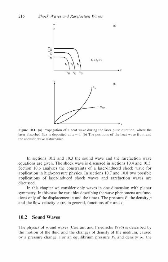
In sections 10.2 and 10.3 the sound wave and the rarefaction waveequations are given. The shock wave is discussed in sections 10.4 and 10.5.Section 10.6 analyses the constraints of a laser-induced shock wave forapplication in high-pressure physics. In sections 10.7 and 10.8 two possibleapplications of laser-induced shock waves and rarefaction waves arediscussed.

In this chapter we consider only waves in one dimension with planarsymmetry. In this case the variables describing the wave phenomena are func-tions only of the displacement x and the time t. The pressure P, the density �and the flow velocity u are, in general, functions of x and t.

10.2 Sound Waves

The physics of sound waves (Courant and Friedrichs 1976) is described bythe motion of the fluid and the changes of density of the medium, causedby a pressure change. For an equilibrium pressure P0 and density �0, the

Figure 10.1. (a) Propagation of a heat wave during the laser pulse duration, where the

laser absorbed flux is deposited at x ¼ 0. (b) The positions of the heat wave front and

the acoustic wave disturbance.


changes in pressure �P and density �� due to the existence of a sound waveare extremely small:

� ¼ �0 þ��;��

�0� 1

P ¼ P0 þ�P;�P

P0

� 1:

ð10:7Þ

It is now assumed that the undisturbed flow velocity is zero and the flowspeed caused by the pressure disturbance is �u, so that

u ¼ u0 þ�u; u0 ¼ 0;�u

cs� 1 ð10:8Þ

where cs is the speed of sound. Using the small perturbations of (10.7) and(10.8), and neglecting second-order quantities in ��, �P and u, the massand momentum equations of (10.1) can be written in the form

@ð��Þ@t

¼ ��0@u

@x; �0

@u

@t¼ � @P

@x: ð10:9Þ

The motion in a sound wave is isentropic, SðxÞ ¼ const., therefore thechange in the pressure is given by

�P ¼�@P

@�

�S

�� c2s��: ð10:10Þ

Differentiating the first equation of (10.9) with respect to time and the secondequation with respect to space, adding the equations and using (10.10), onegets the wave equation

@2ð��Þ@t2

� c2s@2ð��Þ@x2

¼ 0: ð10:11Þ

From this equation it is evident that cs is the velocity of the �� disturbance,which is defined as the velocity of the sound wave. The pressure change �Pand the flow velocity u satisfy a similar wave equation. Equation (10.11) hastwo families of solutions f and g:

��

�P

�u

9>=>; � f ðx� cstÞ and gðxþ cstÞ ð10:12Þ

where the speed of sound is

cs ¼ þ

ffiffiffiffiffiffiffiffiffiffiffiffiffiffiffiffi�@P

@�

�S

s: ð10:13Þ

The disturbances f ðx� cstÞ are moving in the positive x direction, whilegðxþ cstÞ propagates in the negative x direction.

Sound Waves 217

For a plasma satisfying an ideal equation of state, where the electrondensity ne ¼ Zni, Z is the ion charge and ni is the ion density, andTe ¼ Ti ¼ T are the electron and ion temperatures, the pressure is given by

P ¼ nekBTe þ nikBTi ¼ niðZ þ 1ÞkBT ¼ �

mi

ðZ þ 1ÞkBT ð10:14Þ

where mi is the ion mass. An adiabatic process is described by

P ¼ P0

��

�0

��; � ¼ CP

CV

ð10:15Þ

where CP and CV are the heat capacities at constant pressure and constantvolume accordingly, and in a fully ionized plasma � ¼ 5

3. The speed ofsound for the ideal gas is

cs ¼��P

�

�1=2¼

��ðZ þ 1ÞkBT

mi

�1=2: ð10:16Þ

If the undisturbed gas is not stationary, then the flow stream carries thewaves. A transformation from the coordinates moving with the flow (velocityu in the þx direction) to the laboratory coordinates means that the soundwave is travelling with a velocity uþ cs in the þx direction and u� cs inthe �x direction. The curves in the x–t plane in the direction of propagationof small disturbances are called characteristic curves. For isentropic flowthere are two families of characteristics described by

Cþ:dx

dt¼ uþ cs; C�:

dx

dt¼ u� cs ð10:17Þ

so that the physical quantities P and � do not change along these stream lines.There is also a characteristic curve C0, where dx=dt ¼ u, not discussed here.The C� characteristics are curved lines in the x–t plane because u and cs are,in general, functions of x and t.

The equations of state describe any thermodynamic variable as a func-tion of two other variables (assuming that the number of particles do notchange). For example, the density � ¼ �ðP;SÞ is a function of the pressureP and entropy S; therefore, for S ¼ const. one gets

� ¼ �ðPÞ; @�

@t¼

�@�

@P

�S

@P

@t¼ 1

c2s

@P

@t;

@�

@x¼ 1

c2s

@P

@x: ð10:18Þ

Using these relations into the mass conservation and the momentumconservation given in (10.1), we get

1

�cs

@P

@tþ u

�cs

@P

@xþ cs

@u

@x¼ 0;

@u

@tþ u

@u

@xþ 1

�

@P

@x¼ 0: ð10:19Þ


Adding and subtracting these two relations yields�@u

@tþ ðuþ csÞ

@u

@x

�þ 1

�cs

�@P

@tþ ðuþ csÞ

@P

@x

�¼ 0

�@u

@tþ ðu� csÞ

@u

@x

�� 1

�cs

�@P

@tþ ðu� csÞ

@P

@x

�¼ 0:

ð10:20Þ

The brackets [ ] in these equations are derivatives along the characteristicsC�. In order to comprehend this statement, we define a curve x ¼ yðtÞ.The derivative of a function Fðx; tÞ along the curve yðtÞ is given by�

dF

dt

�y

¼ @F

@tþ @F

@x

dx

dt¼ @F

@tþ y 0 @F

@x

dF ¼ð �

dF

dt

�y

dt; x ¼ yðtÞ; y 0 � dx

dt:

ð10:21Þ

For example, for the derivative of F along x ¼ constant one has y 0 ¼ 0,along a stream line y 0 ¼ u, along the characteristic Cþ we have y 0 ¼ uþ cs,etc. Therefore, equations (10.20) and (10.21) can be rewritten as

dJþ � duþ 1

�csdP ¼ 0 along Cþ

�dx

dt¼ uþ cs

�

dJ� � du� 1

�csdP ¼ 0 along C�

�dx

dt¼ u� cs

�:

ð10:22Þ

These equations describe an isentropic flow in one dimension with planarsymmetry. dJ� are total differentials and can be integrated:

Jþ ¼ uþðdP

�cs¼ uþ

ðcs d�

�; J� ¼ u�

ðdP

�cs¼ u�

ðcs d�

�ð10:23Þ

for the second relation on the right-hand side of these equations (10.10) hasbeen used. Jþ and J� are called Riemann invariants and are occasionally usedto solve numerically the flow equations for (and only for) an isentropicprocess, since Jþ and J� are constants along the characteristics Cþ and C�respectively. For a non-isentropic flow the density and the speed of soundare functions of two variables, dJþ and dJ� are not total differentials, andtherefore Jþ and J� have no physical (or mathematical) meaning.

10.3 Rarefaction Waves

We now analyse the case where the pressure is suddenly dropped in anisentropic process, e.g. after the high-power laser is switched off and theablation pressure drops. Another interesting case is after the laser-inducedhigh-pressure wave has reached the back of a target and at the interface

Rarefaction Waves 219

with the vacuum there is a sudden drop in pressure. In these cases, if onefollows the variation in time for a given fluid element, one gets

D�

Dt< 0;

DP

Dt< 0;

D

Dt� @

@tþ u

@

@x: ð10:24Þ

We consider the behaviour of a gas caused by a receding piston (figure 10.2a)in order to visualize the phenomenon of a rarefaction wave. In this figure thepiston is moving in the�x direction so that the gas is continually rarefied as itflows (in the �x direction). The disturbance, called a rarefaction wave, ismoving forward, in the þx direction. One can consider the rarefactionwave to be represented by a sequence of jumps d�, dP, du, etc., so that wecan use the Riemann invariant in order to solve the problem. The forwardrarefaction wave moves into an undisturbed material defined by pressureP0, density �0, flow u0 and the speed of sound cs0 . Using (10.23) we get

u� u0 ¼ðPP0

dP

�cs¼

ð��0

cs d�

�rarefaction moving in þx direction

u� u0 ¼ �ðPP0

dP

�cs¼ �

ð��0

cs d�

�rarefaction moving in �x direction:

ð10:25ÞAs an example we calculate some physical quantities for a rarefaction wave inan ideal gas. Since in a rarefaction wave the entropy is constant, one has the

Figure 10.2. A forward moving rarefaction wave. The propagation velocity of the

rarefaction wave at each point is uþ cs.


following relation between the pressure, the density and the speed of sound(see equations (10.15) and (10.16)):

P

P0

¼��

�0

��;

cscs0

¼��

�0

�ð��1Þ=2: ð10:26Þ

Substituting (10.26) into (10.25) and doing the integral, one gets

u� u0 ¼ð��0

cs d�

�¼ðcscs0

2 dcsð� � 1Þ ¼

2

ð� � 1Þ ðcs � cs0Þ

) cs ¼ cs0 þ 12 ð� � 1Þðu� u0Þ: ð10:27Þ

In this example the piston is moving in the�x direction and at the gas–pistoninterface, and the gas velocity is the same as the piston velocity which has anegative value. The absolute value of the negative gas flow velocity is limitedsince the speed of sound is positive, i.e.

cs0 þ 12ð� � 1Þðu� u0Þ � 0 )

2cs0ð� � 1Þ � �uþ u0 � �u ¼ juj: ð10:28Þ

From equation (10.27) it is evident that the speed of sound is decreased sinceu is negative. This implies, according to equations (10.26), that the densityand the pressure are decreasing, as expressed mathematically in (10.24)and shown schematically in figure 10.2(b).

10.4 Shock Waves

The development of singularities, in the form of shock waves, in a waveprofile due to the nonlinear nature of the conservation equations (10.1) hasalready been discussed by B. Riemann, W. J. M. Rankine and H. Hugoniotin the second half of the 19th century (1860–1890).

A shock wave is created in a medium that suffers a sudden impact (e.g. acollision between an accelerated foil and a target) or in a medium thatreleases large amounts of energy in a short period of time (e.g. highexplosives). When a pulsed high-power laser interacts with matter, veryhot plasma is created. This plasma exerts a high pressure on the surroundingmaterial, leading to the formation of an intense shock wave, moving into theinterior of the target. The momentum of the out-flowing plasma balancesthe momentum imparted to the compressed medium behind the shockfront. The thermal pressure together with the momentum of the ablatedmaterial drives the shock wave.

It is convenient to analyse a shock wave by inspecting a gas compressedby a piston, moving into it with a constant velocity u. The medium hasinitially (the undisturbed medium) a density �0 and a pressure P0, and it isat rest, u0 ¼ 0. A shock wave starts moving into the material with a velocity

Shock Waves 221

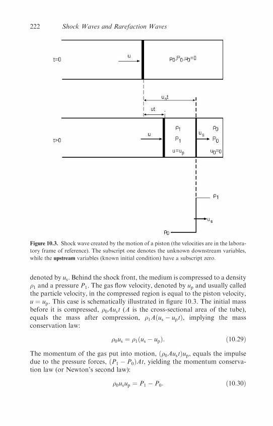
denoted by us. Behind the shock front, the medium is compressed to a density�1 and a pressure P1. The gas flow velocity, denoted by up and usually calledthe particle velocity, in the compressed region is equal to the piston velocity,u ¼ up. This case is schematically illustrated in figure 10.3. The initial massbefore it is compressed, �0Aust (A is the cross-sectional area of the tube),equals the mass after compression, �1Aðus � uptÞ, implying the massconservation law:

�0us ¼ �1ðus � upÞ: ð10:29Þ

The momentum of the gas put into motion, ð�0AustÞup, equals the impulsedue to the pressure forces, ðP1 � P0ÞAt, yielding the momentum conserva-tion law (or Newton’s second law):

�0usup ¼ P1 � P0: ð10:30Þ

Figure 10.3. Shock wave created by the motion of a piston (the velocities are in the labora-

tory frame of reference). The subscript one denotes the unknown downstream variables,

while the upstream variables (known initial condition) have a subscript zero.


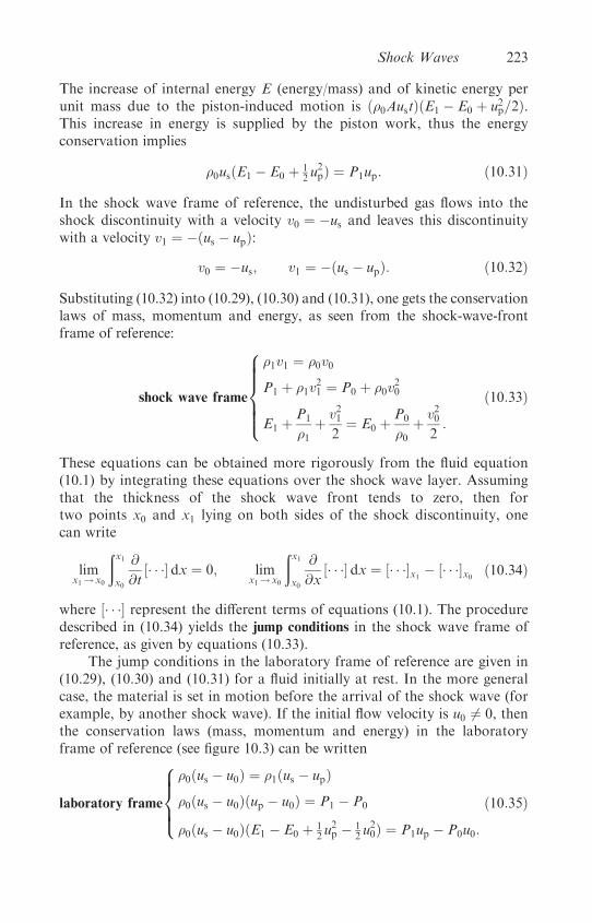
The increase of internal energy E (energy/mass) and of kinetic energy perunit mass due to the piston-induced motion is ð�0AustÞðE1 � E0 þ u2p=2Þ.This increase in energy is supplied by the piston work, thus the energyconservation implies

�0usðE1 � E0 þ 12 u

2pÞ ¼ P1up: ð10:31Þ

In the shock wave frame of reference, the undisturbed gas flows into theshock discontinuity with a velocity v0 ¼ �us and leaves this discontinuitywith a velocity v1 ¼ �ðus � upÞ:

v0 ¼ �us; v1 ¼ �ðus � upÞ: ð10:32Þ

Substituting (10.32) into (10.29), (10.30) and (10.31), one gets the conservationlaws of mass, momentum and energy, as seen from the shock-wave-frontframe of reference:

shock wave frame

�1v1 ¼ �0v0

P1 þ �1v21 ¼ P0 þ �0v

20

E1 þP1

�1þ v21

2¼ E0 þ

P0

�0þ v20

2:

8>>>>><>>>>>:

ð10:33Þ

These equations can be obtained more rigorously from the fluid equation(10.1) by integrating these equations over the shock wave layer. Assumingthat the thickness of the shock wave front tends to zero, then fortwo points x0 and x1 lying on both sides of the shock discontinuity, onecan write

limx1!x0

ðx1x0

@

@t½� � ��dx ¼ 0; lim

x1!x0

ðx1x0

@

@x½� � �� dx ¼ ½� � ��x1 � ½� � ��x0 ð10:34Þ

where ½� � �� represent the different terms of equations (10.1). The proceduredescribed in (10.34) yields the jump conditions in the shock wave frame ofreference, as given by equations (10.33).

The jump conditions in the laboratory frame of reference are given in(10.29), (10.30) and (10.31) for a fluid initially at rest. In the more generalcase, the material is set in motion before the arrival of the shock wave (forexample, by another shock wave). If the initial flow velocity is u0 6¼ 0, thenthe conservation laws (mass, momentum and energy) in the laboratoryframe of reference (see figure 10.3) can be written

laboratory frame

�0ðus � u0Þ ¼ �1ðus � upÞ

�0ðus � u0Þðup � u0Þ ¼ P1 � P0

�0ðus � u0ÞðE1 � E0 þ 12 u

2p � 1

2 u20Þ ¼ P1up � P0u0:

8>>><>>>:

ð10:35Þ

Shock Waves 223

Equations (10.34) or (10.35) are occasionally called the Rankine–Hugoniotrelations. The Hugoniot relations are used to determine the state of thecompressed solid behind the shock front. Assuming that the initial state iswell defined and the quantities E0, u0, P0 and �0 are known, one has fiveunknowns E1, up, P1, �1 and us with three equations (10.35). Usually theshock-wave velocity is measured experimentally, and if the equation ofstate is known (in this case one has four equations), E ¼ EðP; �Þ, then thequantities of the compressed state can be calculated. If the equation ofstate is not known, then one has to measure experimentally two quantitiesof the shocked material, for example us and up, in order to solve the problem.

From the first two equations of (10.33) and using (10.32), the followinggeneral relations can be written:

v0v1

¼ �1�0

� V0

V1

; V � 1

�

v0 ¼ V0

�P1 � P0

V0 � V1

�1=2¼ jusj

v1 ¼ V1

�P1 � P0

V0 � V1

�1=2

v0 � v1 ¼ ½ðP1 � P0ÞðV0 � V1Þ�1=2 ¼ jupj:

ð10:36Þ

Substituting v0 and v1 from these relations into the third relation of (10.33),one gets

E1ðV1;P1Þ � E0ðV0;P0Þ ¼ 12 ðP1 þ P0ÞðV0 � V1Þ: ð10:37Þ

The thermodynamic relation EðV ;PÞ is the equation of state of the materialunder consideration, and assuming knowledge of this function, then equa-tion (10.37), yields a graph (the notation of P1 is changed to PH and V1 is V):

PH ¼ PHðV ;V0;P0Þ: ð10:38Þ

This curve is known in literature as the Hugoniot curve. The Hugoniot curve,shown schematically in figure 10.4(a), is a two-parameter (V0;P0Þ family ofcurves, so that for each initial condition (V0;P0) there is a different curve.The Hugoniot curve is not a thermodynamic function, it does not showthe pressure–volume (or density) trajectory of a shock wave development,but it is a plot of all possible final shocked (compressed) states for agiven initial state (V0;P0). For example, the Hugoniot curve is differentfrom the isentropic curves of the pressure PSðV ;SÞ, which describe thethermodynamic trajectory of pressure–volume (or density) for any givenentropy S. In figure 10.4(a) two isentropes and one isotherm are also plottedschematically. It is interesting to note that for a given final pressure thecompression is higher for an isentrope relative to the Hugoniot, and theisothermal compression is the highest.


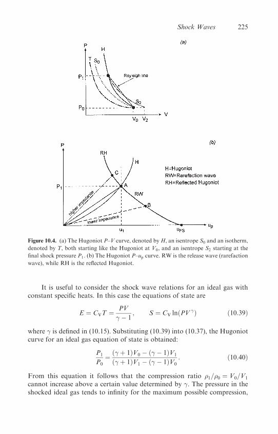
It is useful to consider the shock wave relations for an ideal gas withconstant specific heats. In this case the equations of state are

E ¼ CVT ¼ PV

� � 1; S ¼ CV lnðPV �Þ ð10:39Þ

where � is defined in (10.15). Substituting (10.39) into (10.37), the Hugoniotcurve for an ideal gas equation of state is obtained:

P1

P0

¼ ð� þ 1ÞV0 � ð� � 1ÞV1

ð� þ 1ÞV1 � ð� � 1ÞV0

: ð10:40Þ

From this equation it follows that the compression ratio �1=�0 ¼ V0=V1

cannot increase above a certain value determined by �. The pressure in theshocked ideal gas tends to infinity for the maximum possible compression,

Figure 10.4. (a) The Hugoniot P–V curve, denoted byH, an isentrope S0 and an isotherm,

denoted by T, both starting like the Hugoniot at V0, and an isentrope S2 starting at the

final shock pressure P1. (b) The Hugoniot P–up curve. RW is the release wave (rarefaction

wave), while RH is the reflected Hugoniot.

Shock Waves 225

given by

P1

P0

! 1 )��1�0

�max

¼�V0

V1

�max

¼ � þ 1

� � 1: ð10:41Þ

For example, the maximum compression caused by a planar shock wave in amedium with � ¼ 5

3 is 4�0.Using equation (10.16), for the speed of sound cs, and equation (10.40),

both for the ideal equation of state fluid, one obtains from (10.36):

M20 �

�uscs0

�2

¼�v0cs0

�2

¼ 1

2�

�ð� � 1Þ þ ð� þ 1ÞP1

P0

�> 1

M21 �

�v1cs1

�2

¼ 1

2�

�ð� � 1Þ þ ð� þ 1ÞP0

P1

�< 1:

ð10:42Þ

The ratio M of the flow velocity to the sound velocity is known as the Mach

number. In the limit of a weak shock wave, defined by P1 � P0, one hasM1 � M0 � 1. However, equations (10.42) yield in general M1 < 1 andM0 > 1. The meaning of these relations is that in the shock frame of refer-ence, the fluid flows into the shock front at a supersonic velocity (M0 > 1)and flows out at a subsonic velocity (M1 < 1). In the laboratory frame ofreference, one has the well-known result that the shock wave propagates ata supersonic speed (with respect to the undisturbed medium), and at asubsonic speed with respect to the compressed material behind the shock.Although this phenomenon has been proven here for an ideal gas equationof state, this result is true for any medium, independent of the equation ofstate (Landau and Lifshitz 1987).

In a shock wave the entropy always increases. For example, in an idealgas, equations (10.39) and (10.40) give the increase in entropy during a shockwave process:

S1 � S0 ¼ Cv ln

�P1V

�1

P0V�0

�

¼�

P0V0

ð� � 1ÞT0

�ln

��P1

P0

��ð� � 1ÞðP1=P0Þ þ ð� þ 1Þð� þ 1ÞðP1=P0Þ þ ð� � 1Þ

��> 0:

ð10:43Þ

The increase in entropy indicates that a shock wave is not a reversibleprocess, but a dissipative phenomenon. The entropy jump of a mediumcompressed by shock wave increases with the strength of the shock wave(defined by the ratio P1=P0). The larger P1=P0, the larger is S1 � S0 ¼ �S.The value of �S is determined by the conservation laws (mass, momentumand energy) and by the equation of state. However, the mechanism of thischange is described by viscosity and thermal conductivity (Zeldovich andRaizer 1966), not discussed in this book.


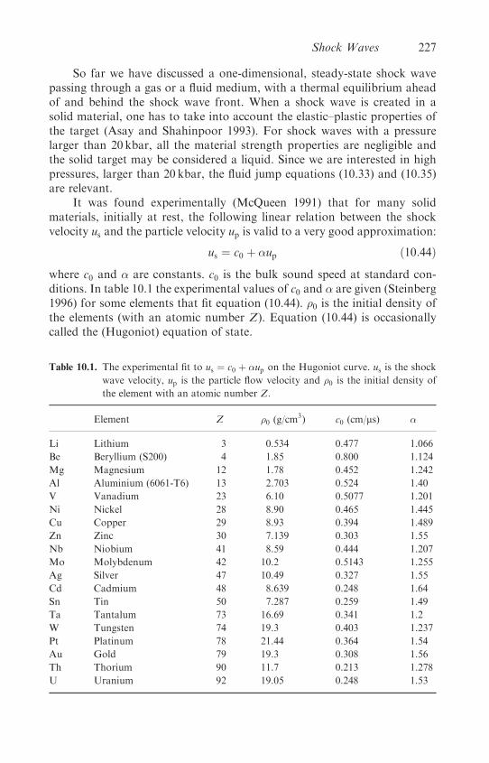
So far we have discussed a one-dimensional, steady-state shock wavepassing through a gas or a fluid medium, with a thermal equilibrium aheadof and behind the shock wave front. When a shock wave is created in asolid material, one has to take into account the elastic–plastic properties ofthe target (Asay and Shahinpoor 1993). For shock waves with a pressurelarger than 20 kbar, all the material strength properties are negligible andthe solid target may be considered a liquid. Since we are interested in highpressures, larger than 20 kbar, the fluid jump equations (10.33) and (10.35)are relevant.

It was found experimentally (McQueen 1991) that for many solidmaterials, initially at rest, the following linear relation between the shockvelocity us and the particle velocity up is valid to a very good approximation:

us ¼ c0 þ �up ð10:44Þ

where c0 and � are constants. c0 is the bulk sound speed at standard con-ditions. In table 10.1 the experimental values of c0 and � are given (Steinberg1996) for some elements that fit equation (10.44). �0 is the initial density ofthe elements (with an atomic number Z). Equation (10.44) is occasionallycalled the (Hugoniot) equation of state.

Table 10.1. The experimental fit to us ¼ c0 þ �up on the Hugoniot curve. us is the shock

wave velocity, up is the particle flow velocity and �0 is the initial density of

the element with an atomic number Z.

Element Z �0 (g/cm3) c0 (cm/ms) �

Li Lithium 3 0.534 0.477 1.066

Be Beryllium (S200) 4 1.85 0.800 1.124

Mg Magnesium 12 1.78 0.452 1.242

Al Aluminium (6061-T6) 13 2.703 0.524 1.40

V Vanadium 23 6.10 0.5077 1.201

Ni Nickel 28 8.90 0.465 1.445

Cu Copper 29 8.93 0.394 1.489

Zn Zinc 30 7.139 0.303 1.55

Nb Niobium 41 8.59 0.444 1.207

Mo Molybdenum 42 10.2 0.5143 1.255

Ag Silver 47 10.49 0.327 1.55

Cd Cadmium 48 8.639 0.248 1.64

Sn Tin 50 7.287 0.259 1.49

Ta Tantalum 73 16.69 0.341 1.2

W Tungsten 74 19.3 0.403 1.237

Pt Platinum 78 21.44 0.364 1.54

Au Gold 79 19.3 0.308 1.56

Th Thorium 90 11.7 0.213 1.278

U Uranium 92 19.05 0.248 1.53

Shock Waves 227

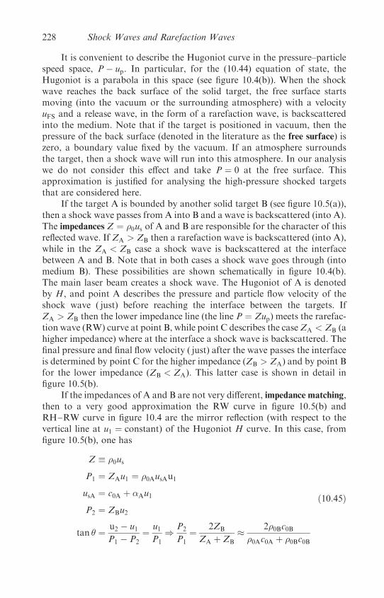
It is convenient to describe the Hugoniot curve in the pressure–particlespeed space, P� up. In particular, for the (10.44) equation of state, theHugoniot is a parabola in this space (see figure 10.4(b)). When the shockwave reaches the back surface of the solid target, the free surface startsmoving (into the vacuum or the surrounding atmosphere) with a velocityuFS and a release wave, in the form of a rarefaction wave, is backscatteredinto the medium. Note that if the target is positioned in vacuum, then thepressure of the back surface (denoted in the literature as the free surface) iszero, a boundary value fixed by the vacuum. If an atmosphere surroundsthe target, then a shock wave will run into this atmosphere. In our analysiswe do not consider this effect and take P ¼ 0 at the free surface. Thisapproximation is justified for analysing the high-pressure shocked targetsthat are considered here.

If the target A is bounded by another solid target B (see figure 10.5(a)),then a shock wave passes from A into B and a wave is backscattered (into A).The impedances Z ¼ �0us of A and B are responsible for the character of thisreflected wave. If ZA > ZB then a rarefaction wave is backscattered (into A),while in the ZA < ZB case a shock wave is backscattered at the interfacebetween A and B. Note that in both cases a shock wave goes through (intomedium B). These possibilities are shown schematically in figure 10.4(b).The main laser beam creates a shock wave. The Hugoniot of A is denotedby H, and point A describes the pressure and particle flow velocity of theshock wave ( just) before reaching the interface between the targets. IfZA > ZB then the lower impedance line (the line P ¼ Zup) meets the rarefac-tion wave (RW) curve at point B, while point C describes the caseZA < ZB (ahigher impedance) where at the interface a shock wave is backscattered. Thefinal pressure and final flow velocity ( just) after the wave passes the interfaceis determined by point C for the higher impedance (ZB > ZA) and by point Bfor the lower impedance (ZB < ZA). This latter case is shown in detail infigure 10.5(b).

If the impedances of A and B are not very different, impedance matching,then to a very good approximation the RW curve in figure 10.5(b) andRH�RW curve in figure 10.4 are the mirror reflection (with respect to thevertical line at u1 ¼ constant) of the Hugoniot H curve. In this case, fromfigure 10.5(b), one has

Z � �0us

P1 ¼ ZAu1 ¼ �0AusAu1

usA ¼ c0A þ �Au1

P2 ¼ ZBu2

tan � ¼ u2 � u1P1 � P2

¼ u1P1

) P2

P1

¼ 2ZB

ZA þ ZB

� 2�0Bc0B�0Ac0A þ �0Bc0B

ð10:45Þ


where the last approximate equality is for weak shock waves. A similar resultis obtained in the case with higher impedance (ZB > ZA).

In figure 10.5(c) a schematic setup of an impedance-matching experi-ment is given. When a shock wave reaches the interface with the vacuum(or the surrounding atmosphere), it irradiates according to the temperatureof the shock wave heated medium. Note that it is a very difficult task to calcu-late the temperature of the shocked medium from the measurement of thisirradiation. If the shock wave temperature is high (about a few thousand

Figure 10.5. (a) A laser induces a shock wave into target A with impedance smaller than

target B. A rarefaction wave (RW) is reflected at the interface A–B. (b) The Hugoniot

curves HA and HB for shock waves in A and B. The reflected rarefaction wave (RW) is

also shown. (c) A schematic setup for an impedance-matching experiment.

Shock Waves 229

K), then the self-illumination may be large enough to be detected by a streakcamera (or other appropriate optical collecting device with a fast informationrecording). If the detecting devices are not sensitive to the self-illuminationthen the measurement of a reflected (diagnostic) laser may be more useful,since the reflection changes significantly with the arrival of the shock wave.The shock wave velocities in A and B are directly measured in this way byrecording the signal of shock breakthrough from the base of A, and fromthe external surfaces of the stepped targets. The time t1 that the shockwave travels through a distance d1 in A, and the time t2 that the shockwave travels through a distance d2 in B, yields the appropriate shock veloci-ties in both targets. Since the initial densities are known, the impedances of Aand B are directly measured. The equation of state of A is known and theHugoniot of A is plotted. Using equations (10.45), P1 is known (from themeasurement of usA) and P2 is directly calculated from the measurementsof both impedances. In this way, the difficult task of measuring two para-meters in the unknown (equation of state) material B is avoided.

As has been shown, it is quite straightforward to measure the shock-wave velocity (assuming that the shock wave is steady, one-dimensionaland the measurement device is very accurate). It is also possible to measureindirectly the particle flow velocity by measuring the free-surface velocity.Accurate optical devices, called VISAR (velocity interferometer system forany reflector) and ORVIS (optically recording velocity interferometersystem) (practically, very fast recording ‘radar’ devices in the opticalspectrum), have been developed to measure accurately the free-surfacevelocity. After the shock wave reaches the back surface of the target, a releasewave with the characteristics of a rarefaction wave is backscattered into thetarget. Since this isentrope is almost the mirror image of the Hugoniot (seefigure 10.4(b); the ‘mirror’ is at u1= constant), one gets

u1 ¼ 12 uFS: ð10:46Þ

Therefore, the measurement of us and uFS determines all the parameters inthe compressed medium (assuming the initial state is accurately known).

The highest laser-induced pressures, 108–109 atm, have been obtainedduring the collision of a target with an accelerating foil. This acceleration wasachieved by laser-produced plasma, or by x-rays from a cavity produced bylaser–plasma interactions. It is therefore now shown how the pressure iscalculated in a planar collision between a flyer and a target.

The flyer has a known (i.e. measured experimentally) initial velocitybefore impact, uf. The initial state before collision is for the target (B),up ¼ 0 and P ¼ 0, while for the flyer (A), up = uf and P ¼ 0. Uponimpact, a shock wave moves forward into B, and another shock wave goesinto the flyer in the opposite direction. The pressure and the particle velocityare continuous at the target–flyer interface. Therefore, the particle velocityof the target changes from zero to u, while the particle velocity in the flyer


changes from uf to u. Moreover, the pressure in the flyer plate A equals thepressure in the target plate B, and if the equations of state are known andgiven by (10.44), and the second equation of (10.35) is used to calculatethe pressure, one gets

PH ¼ �0Buðc0B þ �BuÞ ¼ �0Aðuf � uÞ½c0A þ �Aðuf � uÞ�: ð10:47Þ

This is a quadratic equation in u, with the following solution:

u ¼ �b�ffiffiffiffiffiffiffiffiffiffiffiffiffiffiffiffiffiffib2 � 4ac

p

2a

a � �0A�A � �0B�B

b � �ðc0A�0A þ c0B�0B þ 2�0A�AufÞ

c � ðc0A�0A þ �0A�AufÞuf:

ð10:48Þ

Once the flow velocity is known, it is substituted into (10.47) to derivethe pressure. If the equation of state of the target is not known, then it isnecessary to measure the shock-wave velocity usB as explained above. Inthis case, the pressure equality in the flyer and the target yields

PH ¼ �0BusBu ¼ �0A½c0A þ �Aðuf � uÞ�ðuf � uÞ: ð10:49Þ

Note that in this equation usB is known. The solution of this equation is

u ¼ uf þ w��w2 þ

��0B

�0A�A

�usBuf

�1=2

w � 1

2�A

�c0A þ �0BusB

�0A

�:

ð10:50Þ

In these types of experiment it is occasionally convenient to measure the free-surface velocity of the target and to also study the dynamic strength ofmaterials, as explained in section 10.8.

We end this section with a short comment on shock-wave stability. Onecan see from (10.26) that different disturbances of density travel with differ-ent velocities, so that the larger the density � the faster the wave travels.Therefore, an initial profile �ðx; 0Þ becomes distorted with time. This istrue not only for the density but also for the pressure Pðx; 0Þ, for the flowvelocity uðx; 0Þ, etc. In this way a smooth function of these parameters willsteepen in time due to the nonlinear effect of the wave propagation (higheramplitudes move faster). Therefore, a compression wave is steepened intoa shock wave because in most solids the sound velocity is an increasingfunction of the pressure. In the laboratory frame of reference, the speed ofa disturbance is the sum of the flow velocity and the sound velocityðcs þ uÞ. Therefore, a higher-pressure disturbance will catch up with thelower-pressure disturbance, causing a sharpening profile of the wave. In

Shock Waves 231

reality there are also dissipative mechanisms such as viscosity and thermaltransport. Therefore, the sharpening profile mechanism can only increaseuntil the dissipative forces become significant, and they begin to cancel outthe effect of increasing sound speed with pressure. When the sum of theseopposing mechanisms cancels out, the wave profile no longer changes intime and it becomes a steady shock wave.

The dissipative phenomena are nonlinear functions of the strain rate(strain is the relative distortion of a solid dl=l and the strain rate isthe time derivative of the strain). Therefore, for very fast laser-inducedphenomena, the rise-time of a shock wave is very small and it can besignificantly less than 1 ns.

As already stated above, a disturbance moves at the speed cs þ u in acompression wave. Therefore, a disturbance behind the shock front cannotbe slower than the shock velocity, because in this case it will not be able tocatch the wave front, and the shock would decay (i.e. the shock is unstableto small disturbances behind it). Similarly, a small compressive disturbanceahead of the shock must move slower than the shock front in order not tocreate another shock wave. Thus the conditions for a stable shock wavecan be summarized as

dcsdP

> 0; cs þ up � us; us > cs0 : ð10:51Þ

The first of these equations states that the speed of sound increases withincreasing pressure. The second equation describes the fact that the shockwave is subsonic (Mach number smaller than one) with respect to theshocked medium. The last equation of (10.51) is the well-known phenom-enon that a shock wave is supersonic (Mach number larger than one) withrespect to the unshocked medium. Using equations (10.13) and (10.36),

cs ¼


@�

�S

s¼ V

ffiffiffiffiffiffiffiffiffiffiffiffiffiffiffiffiffiffiffiffi��@P

@V

�S

s; us ¼ V0

ffiffiffiffiffiffiffiffiffiffiffiffiffiffiffiffiffiP1 � P0

V0 � V1

sð10:52Þ

one gets from the last of equations (10.51) the following shock stabilitycriterion:

P1 � P0

V0 � V1

> ��@P

@V

�S;0

: ð10:53Þ

This inequality states that the slope of the Rayleigh line (figure 10.4(a)) is largerthan the slope of the isentrope at the initial state. Similarly, one can show thatthe second of equations (10.51) yields the criterion that the Hugoniot at thefinal state (denoted by 1) must be steeper than the Rayleigh line:

P1 � P0

V0 � V1

��dP

dV

�H;1

: ð10:54Þ


It is important to point out that these criteria are not always satisfied. Forexample, the speed of sound of fused silica decreases with pressure in adomain of low pressures, so that in this case the shock wave is not stable.Moreover, in the regime of phase transitions (solid–solid due to change insymmetry or solid–liquid), the shock wave can split into two or moreshock waves. However, in these cases the stability criteria can be satisfiedfor each individual shock wave.

10.5 Shock Waves in the Presence of Magnetic Fields

Megagauss magnetic fields are easily achieved in laser plasma interactions(see chapter 8). These large magnetic fields, which are created in thecorona, have a large pressure:

PBðMbarÞ � 0:04½BðMgaussÞ�2: ð10:55Þ

The magnetic fields do not penetrate into the solid on the time scale of theshock-wave transient. Since we are mainly interested in the high pressures(Mbar) achieved in the solid target, it appears that the high magneticfields in the corona do not play any important role. However, if shockwaves are created in the corona, or between the critical surface and the abla-tion surface, then the magnetic pressure, the thermal pressure and the shock-wave pressure might be comparable:

� � PT

PB

� 4

�ne

1020 cm�3

��Te

keV

��MGauss

B

�2

: ð10:56Þ

For small magnetic fields, � � 1, the magnetic fields are not important.However, for � � 1 or smaller, a state that is possible to achieve with afew megagauss magnetic field, the creation of a shock wave requires theanalysis of shock waves in the presence of a magnetic field.

Since the magnetic field has in general a direction not parallel to theshock-wave velocity, it is necessary to consider the directions normal andparallel to the shock-wave front (the discontinuity). In the following theshock-wave (front) frame of reference is used. The normal components tothe shock front are denoted by a subscript ‘n’, while the tangential compo-nents (i.e. the components parallel to the shock-wave surface) have thesubscript ‘t’. As in the previous section, the variables before the shock(upstream) and after the shock (downstream) get the subscript 0 and 1respectively. In this case one has the following jump equations (across theshock-wave discontinuity):

(a) mass conservation;(b) momentum conservation normal and parallel to the shock front;

Shock Waves in the Presence of Magnetic Fields 233

(c) energy conservation; and(d) continuity (over the shock front) of the normal magnetic induction field

Bn and of the parallel electric field Et.

We use the magneto-hydrodynamic equations (in Gaussian units) to deriveconservation laws in the form

@

@t½X� þ r � � ¼ 0

limV!0

ðððV

@

@t½X � ¼ 0 )

ðððVr � � dV ¼ �

ððA� � n dA ¼ 0

) ð�0 � �1Þ � n � ½� � n� ¼ 0

ð10:57Þ

where V is a volume containing the shock wave singularity, A is the areaenclosing the volume V (Gauss divergence theorem) and n is a unit vectorperpendicular to the area under consideration. The area A is taken as asmall box surrounding the shock front, where the thickness of the boxtends to zero (therefore V goes to zero). In this case only the two faceswith directions n and �n, on either side of the shock front, contribute tothe integral. �0 and �1 are the values of � on either side of the shock surface(the discontinuity). The end result of the class of equations (10.57) is the jumpconditions across the shock wave front.

The Maxwell equation, which describes the fact that there are nomagnetic poles, gives immediately a jump condition:

r � B ¼ 0 ) ðB0 � B1Þ � n ¼ 0 ) B0n ¼ B1n: ð10:58Þ

Another Maxwell equation, together with the zero Lorentz forceðEþ v B=c ¼ 0Þ, yields

@B

@t¼ �cr E ¼ r ðv BÞ ¼ r � ðBv� vBÞ ¼ 0

) ½ðBv� vBÞ � n� ¼ 0 ) ½Btvn � vtBn� ¼ 0

) B0tv0n � v0tB0n ¼ B1tv1n � v1tB1n

ð10:59Þ

a new jump condition. This equation is the continuity of the tangentialcomponent of the electric field (note that E ¼ B v=c in the presentapproximation).

The mass conservation is directly derived in the usual form:

@�

@tþr � ð�vÞ ¼ 0 ) ½�v � n� ¼ 0 ) �0v0n ¼ �1v1n: ð10:60Þ


The momentum jump conditions (two equations) are obtained from thefollowing combined momentum and Maxwell equations:

�dv

dt¼ �rPþ 1

cJ B

r B ¼ 4�

cJ

) �dv

dt¼ �rPþ 1

4�ð� 1

2rB2 þ B � rBÞ:

ð10:61Þ

The following identities, derived by using (10.58) and (10.60),

r � ð�vvÞ ¼ �v � rv� v@�

@t¼ �

dv

dt� @

@tð�vÞ; r � ðBBÞ ¼ B � rB ð10:62Þ

are used in (10.61) in order to derive the momentum equation in thefollowing form (it is more convenient to use these identities in this newequation in order to derive (10.61)):

@

@tð�vÞ þ r �

��vv� 1

4�BBþ I

�Pþ B2

8�

��¼ 0 ð10:63Þ

where vv and BB are tensors of the second rank (i.e. matrices with com-ponents vivj, BiBj , i; j ¼ 1; 2; 3 in Cartesian coordinates), and I is the unitmatrix (with components i j ¼ 1 for i ¼ j and zero for i 6¼ j, so thatr � ðI Þ ¼ r Þ. This equation is in the desired form of (10.57), yieldingthe momentum jump conditions:��

�vv� 1

4�BB

�� n�þ��

Pþ B2

8�

�n

�¼ 0

)

��v2n þ Pþ B2

t

8�

�¼ 0

��vtvn �

BtBn

4�

�¼ 0:

8>>>><>>>>:

ð10:64Þ

The two relations were obtained for the normal and tangential components(the jump condition for Bn has been used in the first relation).

The last equation to be obtained is the energy relation. In section 3.1(equation 3.19), the following energy conservation is derived:

@

@t

��

�"þ 1

2v2��

þr ��v

�"þ P

�þ 1

2v2��

� E � J ¼ 0 ð10:65Þ

where the transport term and the external forces are neglected. The problemnow is to write the Joule heating term in a format required by a conservationlaw (like the first two terms of (10.65)). Using E and J from equations (10.59)

Shock Waves in the Presence of Magnetic Fields 235

and (10.61). the Joule heating term can be written in the following way:

�E � J ¼ 1

4�½ðv BÞ � r B�

¼ 1

4�½B � ðv � rÞB� v � ðB � rÞB�: ð10:66Þ

Using (10.59) (multiplied by B) and vector algebra, the following identity isderived:

d

dt

�B2

2

�¼ B2r � v� BðB � rÞv

) @

@t

�B2

2

�¼ B2r � v� BðB � rÞv� v � r

�B2

2

�: ð10:67Þ

Using the identity (10.67) in (10.66), we can write

�E � J ¼ @

@t

�B2

8�

�þ 1

4�r � ½B2

v� ðB � vÞB�: ð10:68Þ

We confirm this identity by an alternative derivation. The energy con-servation of the electromagnetic field in a medium is (see Appendix A,equations (A.10) and (A.14), in Gaussian units)

@

@t

�B2

8�

�þr �

�c

4�E B

�¼ �J � E ð10:69Þ

where the D � E ¼ "E2 (" is the dielectric coefficient) is neglected. Thisequation together with

Eþ v B

c¼ 0; ðB vÞ B ¼ B2

v� ðB � vÞB ð10:70Þ

yields equation (10.68).Substituting (10.68) into (10.65) gives the energy equation in the desired

form for the jump condition across the shock wave:

@

@t

��

�"þ 1

2v2 þ B2

8�

��þr �

��v

�"þ P

�þ 1

2v2�þ 1

4�½B2

v� ðB � vÞB��

¼ 0

)��v

�"þ P

�þ 1

2v2�þ 1

4�½B2

v� ðB � vÞB�� n�¼ 0

)�"þ P

�þ 1

2ðv2n þ v2t Þ þ

B2t

4�� vtBtBn

4�

�¼ 0: ð10:71Þ

In summary, the jump equations derived above are: (10.58), (10.59), (10.60),(10.64) and (10.71). The shock-wave surface is at an angle � relative to themagnetic induction B, i.e. the shock front propagates with an angle � relative


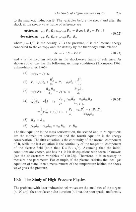
to the magnetic induction B. The variables before the shock and after theshock in the shock-wave frame of reference are

upstream: �0;P0;E0; v0n; v0t;B0n ¼ B cos �;B0t ¼ B sin �

downstream: �1;P1;E1; v1n; v1t;B1n;B1t

ð10:72Þ

where � ¼ 1=V is the density, P is the pressure, E is the internal energyconnected to the entropy and the density by the thermodynamic relation

dE ¼ T dS � P dV ð10:73Þ

and v is the medium velocity in the shock-wave frame of reference. Asshown above, one has the following six jump conditions (Thompson 1962,Shkarofsky et al. 1966):

ð1Þ �0v0n ¼ �1v1n

ð2Þ P0 þ �0v20n þ

B20t

8�¼ P1 þ �1v

21n þ

B21t

8�

ð3Þ �0v0nv0t �B0nB0t

4�¼ �1v1nv1t �

B1nB1t

4�

ð4Þ 1

2ðv20n þ v20tÞ þ "0 þ

P0

�0þ v0nB

20t � v0tB0nB0t

4��0v0n

¼ 1

2ðv21n þ v21tÞ þ "1 þ

P1

�1þ v1nB

21t � v1tB1nB1t

4��1v1n

ð5Þ B0n ¼ B1n

ð6Þ v0nB0t � v0tB0n ¼ v1nB1t � v1tB1n:

ð10:74Þ

The first equation is the mass conservation, the second and third equationsare the momentum conservation and the fourth equation is the energyconservation. The fifth equation is the continuity of the normal componentof B, while the last equation is the continuity of the tangential componentof the electric field (note that E ¼ B v=c). Assuming that the initialconditions are known, one has in (10.74) six equations with seven unknowns(see the downstream variables of (10.72)). Therefore, it is necessary tomeasure one parameter. For example, if the plasma satisfies the ideal gasequation of state, then a measurement of the temperature behind the shockwave gives the pressure.

10.6 The Study of High-Pressure Physics

The problems with laser-induced shock waves are the small size of the targets(100 mm), the short laser pulse duration (1 ns), the poor spatial uniformity

The Study of High-Pressure Physics 237

of a coherent electromagnetic pulse (the laser), and therefore the non-uniformity of the created pressure. All these difficulties have been addressedin the literature and the subject of laser-induced shock wave research hasbeen developed significantly. The critical problems are summarized belowand their possible solutions are discussed.

(a) The planarity (one-dimensional) of the shock wave regardless of thelaser irradiance non-uniformity.

(b) Steady shock wave during the diagnostic measurements in spite of thelaser short-pulse duration.

(c) Well-known initial conditions of the shocked medium. This is requiredto control (i.e. to avoid) the fast electron and x-ray preheating.

(d) Good accuracy (1%) of the measurements.

The planarity of the shock wave is achieved by using optical smoothingtechniques (Lehmberg and Obenschain 1983, Kato et al. 1984, Skupskyet al. 1989, Koenig et al. 1994, Batani et al. 1996). With these devices thelaser is deposited in the target uniformly, within 2% of energy deposition.For example (Lehmberg and Obenschain 1983), one technique denoted as‘induced spatial incoherence’ (ISI) consists of breaking each laser beaminto a large number of beamlets by reflecting the beam off a large numberof echelons. The size of each beamlet is chosen in such a way that its diffrac-tion-limited spot size is about the target diameter. All of the beamlets areindependently focused and overlapped on the target. Another technique(Kato et al. 1984) divides the beam into many elements that have arandom phase shift. This is achieved by passing the laser beam through aphase plate with a randomly phase-shifted mask.

The focal spot of the laser beam on target has to be much larger thanthe target thickness in order to achieve a one-dimensional steady-stateshock wave. In figure 10.6 one can see a schematic profile of a planartarget with thickness d, irradiated by a laser with a focal spot area ¼ �R2

L.A lateral rarefaction wave enters the shocked area and reduces the pressureand density of the shocked area. This effect distorts the one-dimensionalcharacter of the wave, since the shock front is bent in such a way that forvery large distances (�d ) the shock-wave front becomes spherical. Therarefaction wave propagates toward the symmetry axis with the speed ofsound cs (in the shock-compressed area), which is larger than the shock-wave velocity us. Therefore, the good (i.e. undisturbed by the rarefactionwave) one-dimensional shock area ¼ �R2

g is limited by

Rg ¼ RL ��d

us

�cs ¼ RL � d tan � RL � d; A � �R2

L � 10d2 ð10:75Þ

where d=us is the time that the shock wave reaches the back surface. There-fore, in order to have a one-dimensional shock wave one requires thatRg � d, implying an RL � 2d at least, so that the laser focal spot area


A � 10d2. This constraint implies very large laser focal spots for thicktargets.

The second constraint requires a steady shock wave, i.e. the shockvelocity has to be constant as it traverses the target. In figure 10.7 one cansee a schematic x–t (space–time) diagram of a laser-induced shock wave.A rarefaction wave (RW), initiated at a time �t � L (the laser pulse dura-tion) after the end of the laser pulse, follows a shock wave (SW) into thetarget. It is necessary that the rarefaction wave does not overtake theshock wave at position x ¼ d (the back surface) during the measurementof the shock-wave velocity, implying L > d=us. For strong shocks, theshock velocity is of the order of the square root of the pressure (see (10.36)or (10.52)), therefore

L >d

us/ dffiffiffiffi

Pp : ð10:76Þ

Hot electrons can appear during the laser–plasma interaction (see section9.6), causing preheating of the target. This preheats the target before theshock wave arrives, therefore ‘spoiling’ the initial conditions for the high-pressure experiment. Since it is not easy to measure accurately the tempera-ture of the target due to this preheating, it is necessary to avoid preheating.By using shorter wavelengths (0.5 mm or less), the fast electron preheat issignificantly reduced. It is therefore required that the target thickness d islarger than the hot electron mean free path �e. Using the scaling law for

Figure 10.6. A planar target profile irradiated by a laser (the target thickness is d ). The

one-dimensional spot area ¼ �R2g (g for ‘good’) in comparison with the laser irradiation

area ¼ �R2L. RW and SW stand for rarefaction wave and shock wave respectively.

The Study of High-Pressure Physics 239

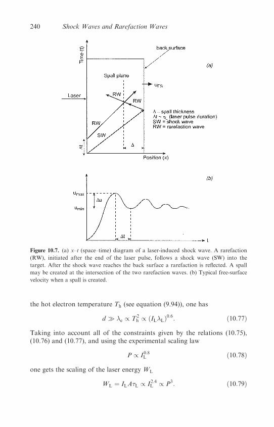
the hot electron temperature Th (see equation (9.94)), one has

d � �e / T2h / ðIL�LÞ0:6: ð10:77Þ

Taking into account all of the constraints given by the relations (10.75),(10.76) and (10.77), and using the experimental scaling law

P / I0:8L ð10:78Þ

one gets the scaling of the laser energy WL

WL ¼ ILAL / I2:4L / P3: ð10:79Þ

Figure 10.7. (a) x–t (space–time) diagram of a laser-induced shock wave. A rarefaction

(RW), initiated after the end of the laser pulse, follows a shock wave (SW) into the

target. After the shock wave reaches the back surface a rarefaction is reflected. A spall

may be created at the intersection of the two rarefaction waves. (b) Typical free-surface

velocity when a spall is created.


Therefore, in order to increase the one-dimensional shock-wave pressureby a factor two, it is necessary to increase the laser energy by an order ofmagnitude.

A more elegant and efficient way to overcome this problem is toaccelerate a thin foil. The foil absorbs the laser, plasma is created (ablation)and the foil is accelerated as in a rocket. In this way, the flyer stores kineticenergy from the laser during the laser pulse duration (the acceleration time)and delivers it, in a shorter time during the collision with a target, in theform of thermal energy. The flyer is effectively shielding the target so thatthe target initial conditions are not changed by fast electrons or by laser-produced x-rays. For these reasons the laser-driven flyer can achieve muchhigher pressures on impact than the directly-laser-induced shock wave(Fabbro et al. 1986, Cauble et al. 1994).

The accuracy of measurements in the study of laser-induced high-pressurephysics require diagnostics with a time resolution better than 100 ps, andoccasionally better than 1 ps, and a spatial resolution of the order of fewmicrons. The accurate measurements of shock-wave speed and particle-flowvelocity are usually obtained with optical devices, including streak camera(Veeser et al. 1979, Cottet et al. 1985, Ng et al. 1987, Evans et al. 1996) andvelocity interferometers (Moshe et al. 1996, Celliers et al. 1998).

10.7 Studies of Equations of State

The phenomena of shock-wave propagation through condensed matterare strongly related to the physics of the equations of state (Altshuler1965, Eliezer et al. 1986, Eliezer and Ricci 1991, Bushman et al. 1993, Eliezeret al. 2002). Atoms in a solid state are attracted to each other at largedistances and repel each other at short distances. At zero temperature andzero pressure the equilibrium is obtained at a specific volume V0c, reachedat the minimum of the (potential) energy. The atoms can be separated to alarge distance by supplying the binding energy (also known as the cohesionenergy) of the order of a few eV/atom, while compressing a condensed matterrequires energy to overcome the repulsive forces.

Small pressures, of the order of 102 atm, can compress a gas to a fewtimes its initial density. However, the compression of a metal by only 10%requires an external pressure (static or shock wave) of the order of105 atm. This is evident from the values of the compressibility at standardconditions 10�6 atm�1, where � is defined by

�S ¼ � 1

V

�@V

@P

�S

: ð10:80Þ

Note that the bulk modulus BS is the inverse of the compressibility,BS ¼ 1=�S.

Studies of Equations of State 241

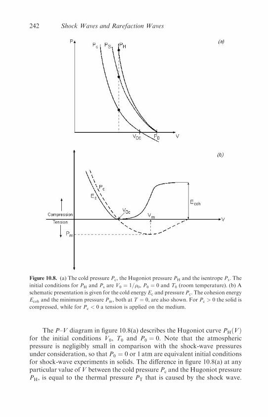
The P–V diagram in figure 10.8(a) describes the Hugoniot curve PHðVÞfor the initial conditions V0, T0 and P0 ¼ 0. Note that the atmosphericpressure is negligibly small in comparison with the shock-wave pressuresunder consideration, so that P0 ¼ 0 or 1 atm are equivalent initial conditionsfor shock-wave experiments in solids. The difference in figure 10.8(a) at anyparticular value ofV between the cold pressure Pc and the Hugoniot pressurePH, is equal to the thermal pressure PT that is caused by the shock wave.

Figure 10.8. (a) The cold pressure Pc, the Hugoniot pressure PH and the isentrope Ps. The

initial conditions for PH and Ps are V0 ¼ 1=�0, P0 ¼ 0 and T0 (room temperature). (b) A

schematic presentation is given for the cold energy Ec and pressure Pc. The cohesion energy

Ecoh and the minimum pressure Pm, both at T ¼ 0, are also shown. For Pc > 0 the solid is

compressed, while for Pc < 0 a tension is applied on the medium.


Since PT is positive, the cold pressure at room temperature is negative,PcðV0Þ < 0. In this figure the isentrope PS that passes through the beginningof the Hugoniot is also shown, so that the mutual positions of PH, PS and Pc

are illustrated.The pressure and the internal energy of a material can be divided into

two contributions:

(a) The temperature-independent term caused by the interaction forcesbetween the atoms of the material. The appropriate pressure Pc andenergy Ec are defined as ‘cold pressure’ and ‘cold energy’ respectively.

(b) The thermal term is usually divided into two parts: one part describesthe motion of the atoms in the lattice, while the second part is due tothe electron thermal motion.

Pa and Ea denote the thermal lattice pressure and energy respectively, and theappropriate electron contributions are Pe and Ee. Therefore, the equation ofstate is usually written in the following form:

PðV ;TÞ ¼ PcðVÞ þ PTðV ;TÞ

PTðV ;TÞ ¼ PaðV;TÞ þ PeðV ;TÞ

EðV ;TÞ ¼ EcðVÞ þ ETðV ;TÞ

ETðV ;TÞ ¼ EaðV;TÞ þ EeðV ;TÞ:

ð10:81Þ

The thermodynamic relation relates the cold pressure and energy:

EcðVÞ ¼ �ðVV0c

PcðVÞ dV : ð10:82Þ

As usual, the potential energy is fixed up to a constant, and this constant hasbeen chosen in such a way that EcðV0cÞ ¼ 0. Note that PcðV0cÞ ¼ 0 is thedefinition of V0c. It has been found that to a good approximation, near theHugoniot curve, the lattice thermal energy and pressure are related throughthe Gruneisen equation of state, and the energy is described by the Debyesolid-state theory:

Ea ¼ CVðT � T0Þ þ E0; PaðV ;TÞ ¼ �aðVÞV

Ea ð10:83Þ

where �a is the Gruneisen coefficient (assumed to be a function of V), CV isthe lattice specific heat at constant volume, T0 is the initial temperature in theshock wave experiment, usually the room temperature, and E0 is the internalenergy at T0, defined by

E0 ¼ðT0

0CVðTÞ dT : ð10:84Þ


At room temperature and for slightly lower and higher temperatures, thespecific heat CV has the Dulong–Petit value

CV ¼ 3R

hAi

�erg

g � deg

�

R ¼ 8:314 107�

erg

mol � deg

�

hAi ¼ average atomic weight

�g

mol

�:

ð10:85Þ

For example, hAi for aluminium and copper is 27 and 63.55 respectively.Assuming for the electron thermal part an equation of state similar to

the Gruneisen equation of state for the lattice, one has

Pe ¼�eV

Ee: ð10:86Þ

To the first approximation, the thermal electron energy is taken from the freeelectron model,

Ee ¼ 12�T

2 ð10:87Þ

and � is related to the specific volume V by the thermodynamic relation,

�@E

@V

�T

¼ T

�@P

@T

�V

� P: ð10:88Þ

Substituting (10.86) and (10.87) into (10.88) yields

@�

@V¼ �e�

V) � ¼ �e exp

�ðVV0

�e dV

V

�

� ¼ �0

�V

V0

�1=2

for �e ¼ 0:5:

ð10:89Þ

The value of �e ¼ 0:5 is a good approximation for many metals up to shock-wave data of a few megabars pressure.

Combining equations (10.81), (10.82), (10.83), (10.86) and (10.89), onegets

P ¼ Pc þ�aV

½CVðT � T0Þ þ E0� þ1

4

��0V0

��V0

V

�1=2

T2

E ¼ �ðV

Pc dVþCVðT � T0Þ þ E0 þ�02

�V

V0

�1=2

T2:

ð10:90Þ


The cold pressure can be described by a polynomial in ðV0c=VÞ1=3 in such away that it fits the experimental values of the bulk modulus, the derivative ofthe bulk modulus at zero pressure, the cohesion energy and the Thomas–Fermi model (or modified models) at very high compressions.

Although the equations of state described in equations (10.90) have 10parameters, they do not describe phase transitions, such as solid to solidwith different symmetry or melting and evaporation. In order to describethese phenomena, many more parameters based on theoretical models andexperimental data are required.

As explained in section 10.4, in a shock-wave experiment one canmeasure the shock-wave velocity (us) and the particle velocity (up). It hasalso been attempted to measure the temperature associated with a shockwave; however, the experimental data so far are not very accurate.

The shock-wave velocity is directly measured in a stepped target(velocity¼measured step length/measured time difference) using an opticalstreak camera. The particle velocity is more difficult to measure, and up isdeduced, for example, from impedance-matching experiments (see section10.4) or by the optical measuring of the free-surface (i.e. back surface)velocity. The measured equation of state is given in the form of the linearus–up equation (10.44). The velocity measurements should have an accuracyof about 1%, in order to give good accuracy (10%) in other variables suchas pressure, energy, etc. It is important to point out that the linear us–uprelation (equation (10.44) and table 10.1), is not always correct for all solidelements.

Sometimes a higher polynomial in up is necessary to fit the experimentaldata. For example (Steinberg 1996),

hafnium: usðcm=msÞ ¼ 0:298þ 1:448up � 3:852

�up

us

�up þ 7:0

�up

us

�2

up

lead: usðcm=msÞ ¼ 0:2006þ 1:429up þ 0:8506

�up

us

�up � 1:64

�up

us

�2

up

titanium: usðcm=msÞ ¼ 0:502þ 1:536up � 5:138

�up

us

�up þ 10:82

�up

us

�2

up:

ð10:91Þ

In the following part of this section, it is shown how one can study thethermodynamic equations of state in the neighbourhood of the Hugoniotfrom the measurements of the shock velocity and the particle velocity. Forsimplicity, the further discussion assumes the linear us–up relation (equation(10.44)), valid for many metals.

It is convenient to define the parameter � related to the compression�=�0, in such a way that � ¼ 0 for no compression and � ¼ 1 for an


infinite �=�0:

� � 1� V

V0

¼ 1� �0�: ð10:92Þ

Using equations (10.36) and (10.44), the particle velocity and the shockvelocity can be presented in the following way:

up

us¼ V0 � V

V0

¼ �

us ¼ c0 þ �up

9>=>; )

up ¼ �c01� ��

us ¼c0

1� ��

:

8>><>>:

ð10:93Þ

Substituting these results into the Hugoniot pressure, one gets PH as afunction of V (or �), the experimentally measured quantities c0 and �, andthe initial condition V0:

PH ¼ �0usup ¼ �c20

V0ð1� ��Þ2¼ c20ðV0 � VÞ

½V0 � �ðV0 � VÞ�2: ð10:94Þ

It is interesting to point out that from this equation the maximum possiblecompression is obtained for an infinite PH, implying

�max

�0¼ �

�� 1: ð10:95Þ

For example (see table 10.1), � of aluminium equals 1.4, implying that in ashock wave the compression �=�0 is smaller than 2.5.

The derivative of this pressure with respect to the specific volume V is

P0H �

�dP

dV

�H

¼ dPH

dV¼ �

�c0V0

�2 1þ ��

ð1� ��Þ3

¼ �c20

�V0 þ �ðV0 � VÞ½V0 � �ðV0 � VÞ�3

�: ð10:96Þ

Using this relation, the bulk modulus on the Hugoniot, BH, is obtained:

BH ¼ �V

�dP

dV

�H

ð10:97Þ

and its derivative with respect to the pressure can also be derived:�dBH

dP

�H

¼�dBH

dV

�H

�dV

dP

�H

¼ ��

dP

dV

�H

þ V

�d2P

dV2

�H

�1

ðdP=dVÞH

¼ ��1þ Vðd2P=dV2ÞH

ðdP=dVÞH

�: ð10:98Þ


Experimentally one measures the bulk modulus at constant entropy andits derivative at V ¼ V0, P ¼ P0 ¼ 0 (the shock wave initial condition).For the Hugoniot pressure and the isentrope PS starting at V ¼ V0,P ¼ P0 ¼ 0, the following relations are valid:�

dPH

dV

�P0;V0

¼�dPS

dV

�P0;V0

;

�d2PH

dV2

�P0;V0

¼�d2PS

dV2

�P0;V0

: ð10:99Þ

From equations (10.96), (10.97), (10.98) and (10.99), the following importantrelations are derived:

BHðP0;V0Þ ¼ BSðP0;V0Þ ¼c20V0

¼ �0c20

B0HðP0;V0Þ ¼ B0

SðP0;V0Þ ¼ 4�� 1:

ð10:100Þ

From shock-wave data (equation of state), one knows c0 and � and thereforethe bulk modulus and its pressure derivative. The last two physicalquantities, BS and dBS=dP ¼ B0

S, are very important in calculating the coldpressure Pc and energy Ec. BS, of the order of 1Mbar, can also be measuredin static experiments thanks to the technological advances in reaching highpressures (up to a few megabars). However, it is difficult to measure B0

S instatic experiments to a good accuracy since this quantity measures thecurvature of the P–V curve. On the other hand, the shock-wave experimentsin this domain of pressure are easily and accurately performed.

We now calculate the speed of sound:

cs ¼


@�

�S

s¼ V

ffiffiffiffiffiffiffiffiffiffiffiffiffiffiffiffiffiffiffiffi��@P

@V

�S

s� V

ffiffiffiffiffiffiffiffiffiffiffiffiffiffiffiffiffiffiffiffi� dPSðVÞ

dV

r: ð10:101Þ

For this purpose one needs the isentrope pressure curve PSðVÞ, which can becalculated from the knowledge of the Hugoniot pressure PHðVÞ using the(ion) Gruneisen equation of state. In order to do so, the electron thermalcontribution Pe should be neglected. For most of the solid materials,Pe � Pa for pressures less than a few hundred kilobars. For example, wedemonstrate this for aluminium at a shock-wave pressure of 580 kbar. Atthis Hugoniot point, the compression is 1.40 and the temperature is1480K. Using the following experimental data at standard conditions

aluminium: V �10 ¼ �0 ¼ 2:70 ½g=cm3�

CV ¼ 8:96 106 ½erg=ðg � degÞ�

BS ¼ 1:36 1012 ½dyne=cm2� ¼ 1:36Mbar

E0 ¼ 107 ½erg=g��a ¼ 2:09

�0 ¼ 500 ½erg=ðg � deg2Þ�

ð10:102Þ


we get from the equations of state (10.90):

aluminium:V0

V¼ �

�0¼ 1:40; TH ¼ 1480K; PH ¼ 580 kbar

) Pc ¼ 495:6 kbar; Pa ¼ 83:5 kbar; Pe ¼ 0:9 kbar:

ð10:103Þ

From this example one can see that even in a shock wave with 580 kbar ofpressure in aluminium, the electronic thermal part contributes about0.15% to the total pressure. Therefore, in the following analysis theelectronic thermal part is neglected.

The Gruneisen equation of state (see (10.83)) can be written in the form

PðV ;EÞ ¼ PcðVÞ þ �aðVÞV

½E � EcðVÞ�: ð10:104Þ

Substituting P ¼ PH in this equation and subtracting it from P, one gets

P� PH ¼ �aV

ðE � EHÞ: ð10:105Þ

For P ¼ PS, the derivative of (10.105) yields (after using dES=dV ¼ �PS)

PS ¼ � dEH

dVþ ðPH � PSÞ

d

dV

�V

�a

�þ V

�a

�dPH

dV� dPS

dV

�: ð10:106Þ

Taking the derivative of the Hugoniot energy relation (10.37) gives

dEH

dV¼

�V0 � V

2

�dPH

dV��P0 þ PH

2

�: ð10:107Þ

Substituting (10.107) into (10.106) yields

dPS

dV¼

�1� �a

2VðV0 � VÞ

�dPH

dVþ �a2V

ðP0 þ PHÞ

þ �aV

ðPH � PSÞd

dV

�V

�a

�� PS

��aV

�: ð10:108Þ

Using equations (10.101) and (10.108) and defining the sound speed on theHugoniot points, i.e. cH is equal to cS for PS ¼ PH, one gets

c2H ¼��aV

2

�PH þ

��aV

2

�ðV0 � VÞ � V2

�dPH

dV

c2S ¼ c2H þ �aVðPS � PHÞ�1þ d

dV

�V

�a

��:

ð10:109Þ

In the second equation of (10.109), the speed of sound cS is along therelease isentrope off the Hugoniot (i.e. an isentrope starting after theshock-wave point with pressure PH). See curve S2 in figure 10.4(a). It was


found experimentally that the Gruneisen coefficient satisfies the relation

�aðVÞV

¼ �0V0

¼ const: ð10:110Þ

Using this relation in (10.109) yields the approximate relation

c2S � c2H þ �0

�V2

V0

�ðPS � PHÞ: ð10:111Þ

Substituting into (10.109) the equations (10.93), (10.94) and (10.96), one getsthe sound speed on the Hugoniot points as a function of measured quantities,� ¼ up=us, c0 and �:

cH ¼ c01� �

ð1� ��Þ3=2

ffiffiffiffiffiffiffi�0�

2

rð1þ �� 0��

2Þ1=2: ð10:112Þ

From equation (10.111), or more accurately from (10.109), the Gruneisenparameter may be determined if the Hugoniot pressure and the speed ofsound are measured experimentally. By placing a transparent materialcoupled to the target under consideration, the rarefaction overtakes theshock wave and reduces significantly the shock pressure. By measuring thisphenomenon, the change in light radiance caused by the decrease in theshock pressure, the speed of sound in the shocked material can be measured.

10.8 Studies of Dynamic Strength of Materials

Spall is a dynamic fracture of materials, extensively studied in ballisticresearch (Rosenberg et al. 1983, Bushman et al. 1993). The term spall, asused in shock wave research, is defined as planar separation of material,parallel to the wave front as a result of dynamic tension perpendicular tothis plane. The reflection of a shock-wave pulse from the rear surface (thefree surface) of a target causes the appearance of a rarefaction wave intothe target. Tension (i.e. negative pressure) is induced within the target bythe crossing of two opposite rarefaction waves, one coming from the frontsurface due to the fall of the input pressure and the second due to reflectionof the shock wave from the back surface (see figure 10.7(a)). If the magnitudeand duration of this tension are sufficient then internal rupture, called spall,occurs. In this section we point out that this type of research can also be donewith laser beams (Gilath et al. 1988, Eliezer et al. 1990, Boustie and Cottet1991, Fortov et al. 1991, De Resseguier and Cottet 1995, Eliaz et al. 2000,Moshe et al. 2000).

Spall in ductile materials is controlled by localized plastic deformationaround small voids that grow and coalesce to form the spall plane. Invery fast phenomena and very high tension, as in high-power pulsed laser

Studies of Dynamic Strength of Materials 249

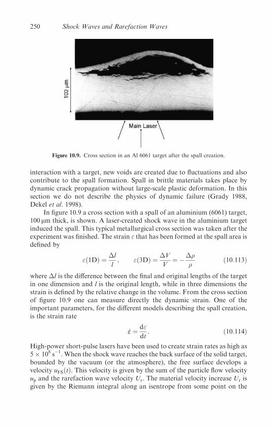
interaction with a target, new voids are created due to fluctuations and alsocontribute to the spall formation. Spall in brittle materials takes place bydynamic crack propagation without large-scale plastic deformation. In thissection we do not describe the physics of dynamic failure (Grady 1988,Dekel et al. 1998).

In figure 10.9 a cross section with a spall of an aluminium (6061) target,100 mm thick, is shown. A laser-created shock wave in the aluminium targetinduced the spall. This typical metallurgical cross section was taken after theexperiment was finished. The strain " that has been formed at the spall area isdefined by

"ð1DÞ ¼ �l

l; "ð3DÞ ¼ �V

V¼ ��

�ð10:113Þ

where �l is the difference between the final and original lengths of the targetin one dimension and l is the original length, while in three dimensions thestrain is defined by the relative change in the volume. From the cross sectionof figure 10.9 one can measure directly the dynamic strain. One of theimportant parameters, for the different models describing the spall creation,is the strain rate

_"" ¼ d"

dt: ð10:114Þ

High-power short-pulse lasers have been used to create strain rates as high as5 108 s�1. When the shock wave reaches the back surface of the solid target,bounded by the vacuum (or the atmosphere), the free surface develops avelocity uFSðtÞ. This velocity is given by the sum of the particle flow velocityup and the rarefaction wave velocity Ur. The material velocity increase Ur isgiven by the Riemann integral along an isentrope from some point on the

Figure 10.9. Cross section in an Al 6061 target after the spall creation.


Hugoniot (pressure PH) to zero pressure (see equations (10.25) and (10.101)):

uFS ¼ up þUr; Ur ¼ðPH

0

dP

�cs¼ð��0

cs d�

�¼ðVðP¼0Þ

VðPHÞ

�� dPS

dV

�1=2

dV :

ð10:115Þ

The derivative dPS=dV is given in equation (10.108), so that knowledge of PS

gives the value of Ur. Layers of the target adjacent to the free surface go intomotion under the influence of the shock-wave transition from V0, P0 ¼ 0 toV, PH, and subsequent isentropic expansion in the reflected rarefaction wavefrom PH,V to P0 ¼ 0, V2 (see figure 10.4(a)), whereV2 > V0. Although thesetwo processes are not the same, it turns out that for up � us one has, to a verygood approximation,

up � Ur ) uFS � 2up: ð10:116Þ

It was found experimentally, for many materials, that this relation is verygood (within 1%) up to shock-wave pressures of about 1Mbar. Therefore,from the free-surface velocity measurements, one can calculate the particleflow velocity of the shock-wave compressed material. This free-surfacevelocity, together with the experimental measurement of the shock-wavevelocity, might serve as the two necessary quantities, out of five (PH,V ¼ 1=�, EH, us, up), to fix a point on the Hugoniot.

A typical free-surface velocity measurement, in the case of the creationof a spall, is given in figure 10.7(b). umax (related to up in the above discussion)in this figure is the maximum free-surface velocity. At later times the free-surface velocity decreases to umin until a second shock arrives from thespall, ‘the new free surface’. When a rarefaction wave reaches the internalrupture of the target (the spall) a shock wave is reflected towards the freesurface, causing an increase in the free-surface velocity. These reverberationphenomena are repeated until the free surface reaches an asymptoticconstant velocity. The spall strength �, i.e. the negative pressure (tension)that a spall occurs, can be calculated using the Riemann invariants

uðP ¼ 0; u ¼ uminÞ � umin ¼ u00 �ð0�

dP

�cs

uðP ¼ 0; u ¼ umaxÞ � umax ¼ u00 þð0�

dP

�cs

9>>>>=>>>>;

) �u � umax � umin ¼ 2

ð0�

dP

�cs:

ð10:117Þ

Assuming that the negative pressure is not too large, then to a goodapproximation � ¼ �0 and cs ¼ c0, implying that the spall strength is

� ¼ � �0c0ðumax � uminÞ2

� � spall: ð10:118Þ


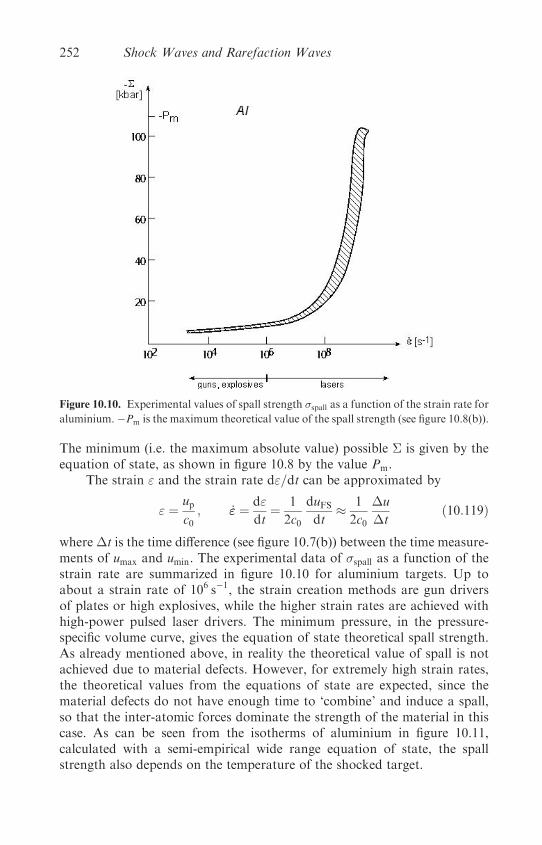
The minimum (i.e. the maximum absolute value) possible � is given by theequation of state, as shown in figure 10.8 by the value Pm.

The strain " and the strain rate d"=dt can be approximated by

" ¼up

c0; _"" ¼ d"

dt¼ 1

2c0

duFSdt

� 1

2c0

�u

�tð10:119Þ

where�t is the time difference (see figure 10.7(b)) between the time measure-ments of umax and umin. The experimental data of spall as a function of thestrain rate are summarized in figure 10.10 for aluminium targets. Up toabout a strain rate of 106 s�1, the strain creation methods are gun driversof plates or high explosives, while the higher strain rates are achieved withhigh-power pulsed laser drivers. The minimum pressure, in the pressure-specific volume curve, gives the equation of state theoretical spall strength.As already mentioned above, in reality the theoretical value of spall is notachieved due to material defects. However, for extremely high strain rates,the theoretical values from the equations of state are expected, since thematerial defects do not have enough time to ‘combine’ and induce a spall,so that the inter-atomic forces dominate the strength of the material in thiscase. As can be seen from the isotherms of aluminium in figure 10.11,calculated with a semi-empirical wide range equation of state, the spallstrength also depends on the temperature of the shocked target.

Figure 10.10. Experimental values of spall strength spall as a function of the strain rate for

aluminium.�Pm is the maximum theoretical value of the spall strength (see figure 10.8(b)).


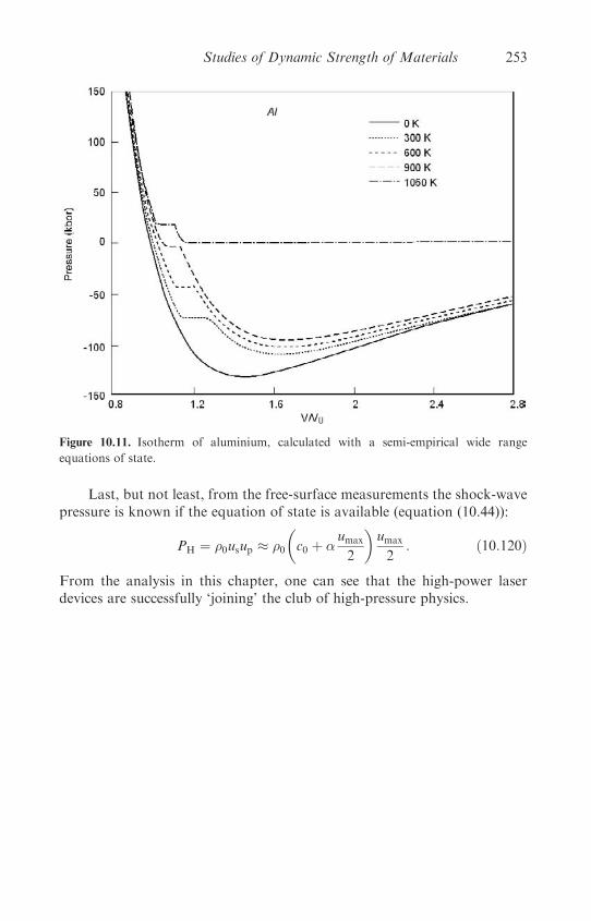
Last, but not least, from the free-surface measurements the shock-wavepressure is known if the equation of state is available (equation (10.44)):

PH ¼ �0usup � �0

�c0 þ �

umax

2

�umax

2: ð10:120Þ

From the analysis in this chapter, one can see that the high-power laserdevices are successfully ‘joining’ the club of high-pressure physics.

Figure 10.11. Isotherm of aluminium, calculated with a semi-empirical wide range

equations of state.


Chapter 11

Hydrodynamic Instabilities

11.1 Background

The Rayleigh–Taylor (RT) instability occurs if a heavy fluid is supported by alight fluid in a gravitational field (Rayleigh 1883). Equivalently, one gets RTinstability when a light fluid pushes and accelerates a heavy fluid (Taylor1950) (see figure 11.1). In general, theRT instability occurswhenever a pressuregradient opposes a density gradient (rP is in an opposite direction to r�).

The hydrodynamic instabilities, and in particular the RT instability,have been reviewed in the literature (Chandrasekhar 1961, Drazin andReid 1981, Kull 1991). Reviews on RT instabilities in laser–plasma inter-actions, with an emphasis on inertial confinement fusion (ICF), are alsoavailable (Bodner 1991, Gamaly 1993, Hoffman 1995).

A sinusoidal wave, with amplitude �, on the surface between the two RTunstable fluids will grow exponentially:

� ¼ �0 exp �0tð Þ; �0 ¼ffiffiffiffiffiffiffiffiffiAka

p; A � �H � �L

�H þ �L; k ¼ 2�

�ð11:1Þ

where � is the wavelength of the sinusoidal wave, a is the acceleration of thetwo fluids (or a ¼ g in the gravitational field, without acceleration), �H and�L are the densities of the heavier and the lighter fluids and A is theAtwood number. �0 is the classical value obtained by Rayleigh, more thana hundred years ago, for two fluids in contact in the gravitational field(a ¼ g in (11.1)).

For example, when a high-power laser interacts with a thin foil, plasmais created and accelerates the foil. In this case one has a low-density medium(the plasma) accelerating a high-density medium (the solid target); therefore,the acceleration is subject to RT instabilities. For a typical high-power laseracceleration of the order of 1015 cm/s2 and a wavelength of the order ofthe foil thickness �100 mm, one gets �0 � 109 s�1, implying that the classicale-folding time is 1=�0 � 1 ns.

254

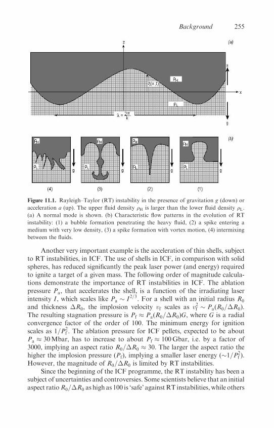
Another very important example is the acceleration of thin shells, subjectto RT instabilities, in ICF. The use of shells in ICF, in comparison with solidspheres, has reduced significantly the peak laser power (and energy) requiredto ignite a target of a given mass. The following order of magnitude calcula-tions demonstrate the importance of RT instabilities in ICF. The ablationpressure Pa, that accelerates the shell, is a function of the irradiating laserintensity I , which scales like Pa � I2=3. For a shell with an initial radius R0

and thickness �R0, the implosion velocity vf scales as v2f � Pa(R0=�R0).The resulting stagnation pressure is Pf � Pa(R0=�R0)G, where G is a radialconvergence factor of the order of 100. The minimum energy for ignitionscales as 1=P2

f . The ablation pressure for ICF pellets, expected to be aboutPa � 30Mbar, has to increase to about Pf � 100Gbar, i.e. by a factor of3000, implying an aspect ratio R0=�R0 � 30. The larger the aspect ratio thehigher the implosion pressure (Pf), implying a smaller laser energy (�1=P2

f ).However, the magnitude of R0=�R0 is limited by RT instabilities.

Since the beginning of the ICF programme, the RT instability has been asubject of uncertainties and controversies. Some scientists believe that an initialaspect ratioR0=�R0 as high as 100 is ‘safe’ againstRT instabilities,while others

Figure 11.1. Rayleigh–Taylor (RT) instability in the presence of gravitation g (down) or

acceleration a (up). The upper fluid density �H is larger than the lower fluid density �L.

(a) A normal mode is shown. (b) Characteristic flow patterns in the evolution of RT

instability: (1) a bubble formation penetrating the heavy fluid, (2) a spike entering a

medium with very low density, (3) a spike formation with vortex motion, (4) intermixing

between the fluids.

Background 255

were predicting that even an aspect ratio of 4 is going to ‘destroy’ the shell(before the desired high compression is achieved) by RT instabilities. Theaspect ratio is a very important parameter for ICF since thicker pellets requirea higher laser intensity to achieve the desired high pressure, and very highlaser intensity could drive unacceptable plasma instabilities (see chapter 6).In addition, thicker shells require a larger amount of laser energy.

The RT instability can cause a disturbance to grow from extremely smallamplitude to a level that can disrupt the flow completely. In the aboveexamples it can break the accelerated foil or the shell before it reaches thedesired final velocity.

The initial disturbance, called the ‘seed’, arises from limitations tofabricate a perfect plane (for foil acceleration) or a perfect spherical shellfor ICF. Small perturbations caused by the roughness of the materialstructures, or by machining marks during the preparation of the target, aresources of instability seeds. Furthermore, the pattern of the laser intensityon the target can imprint a disturbance on an initially perfect smoothtarget. Since these types of disturbance are facts of reality, one has to calcu-late the constraints on the target smoothness and on the laser uniformityfrom the hydrodynamic instability theory.

Any initial perturbation can be described as an infinite series (e.g. aFourier series) of normal modes (with wavelength � ¼ L=j, j ¼ 1; 2; 3; . . .).Any given mode is not growing to infinity by the RT instability, but isexpected to saturate at a finite amplitude (��=2). On their route to satura-tion, perturbations with wavelength greater than the fluid thickness woulddestroy the flow (break the foil or the shell).

The shorter wavelength modes reach saturation before the longerwavelength modes (see equation (11.1), �0 � ða=�Þ1=2). After the shorterwavelength modes stop growing, they transfer their acquired energy to thelonger wavelength disturbances, and the small disturbances are convertedinto larger structures. It turns out that these structures have the topologyof bubbles and spikes. The lighter fluid penetrates the heavier fluid in theform of bubbles, and spikes of the heavier fluid enter the lighter fluid.Characteristic flow patterns in the evolution of RT instability are shown infigure 11.1(b), where a bubble formation penetrating the heavy fluid isshown together with possible spikes entering the lighter medium. Aschematic spike formation with vortex motion and late intermixing betweenthe fluids are also shown in this figure.

The saturation mechanism can be understood (Shvarts et al. 1995) bythe existence of a nonlinear drag force:

Fd � ��dSu2: ð11:2Þ

The ambient fluid for bubbles is the heavy liquid and the ambient fluid forspikes is the light fluid; therefore, �d ¼ �H for bubbles and �d ¼ �L forspikes. S is the area and u the velocity of the bubbles or the spikes. Equating

256 Hydrodynamic Instabilities

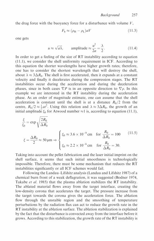
the drag force with the buoyancy force for a disturbance with volume V ,

Fb � �H � �Lð ÞaV ð11:3Þ

one gets

u �ffiffiffiffiffiffia�

p; amplitude � u2

2a¼ �

2: ð11:4Þ

In order to get a feeling of the size of RT instability according to equation(11.1), we consider the shell uniformity requirement in ICF. According tothis equation the shorter wavelengths have higher growth rates; therefore,one has to consider the shortest wavelength that will destroy the shell,about � � 3�R0. The shell is first accelerated, then it expands at a constantvelocity and finally it decelerates during the compression stages. The RTinstabilities occur during the acceleration and during the decelerationphases, since in both cases rP is in an opposite direction to r�. In thisexample we are interested in the RT instability during the accelerationphase. As an order of magnitude estimate, one can assume that the shellacceleration is constant until the shell is at a distance R0=2 from thecentre, R0=2 � 1

2 at2. Using this relation and � � 3�R0, the growth of an

initial amplitude �0 for Atwood number �1 is, according to equation (11.1),

�

�0¼ exp

ffiffiffiffiffiffiffiffiffiffi2R0

�R0

s

� ¼ �R0

2� 50 mm )

�0 � 3:6� 10�9 cm forR0

�R0

¼ 100

�0 � 2:2� 10�6 cm forR0

�R0

¼ 30:

8>>><>>>:

ð11:5Þ

Taking into account the pellet fabrication and the laser initial imprint on theshell surface, it seems that such initial smoothness is technologicallyimpossible. Therefore, there must be some mechanism that reduces the RTinstabilities significantly or all ICF schemes would fail.

Following the Landau–Lifshitz analysis (Landau and Lifshitz 1987) of achemical burn front of a weak deflagration, it was suggested (Bodner 1974,Takabe et al. 1985) that the plasma ablation stabilizes the RT instability.The ablated material flows away from the target interface, creating thelow-density corona that accelerates the target. The pressure increase fromthe target towards the corona gives the acceleration force. The ablationflow through the unstable region and the smoothing of temperatureperturbations by the radiation flux can act to reduce the growth rate in theRT instability at the ablation surface. The ablation stabilization is explainedby the fact that the disturbance is convected away from the interface before itgrows. According to this stabilization, the growth rate of the RT instability is

Background 257

effectively reduced to

� ¼ �ffiffiffiffiffika

p� �kua; ua ¼

1

�max

dm

dt

� �; � � 0:9; � � 3 ð11:6Þ

where �max is the peak density at the interface and dm/dt is the mass (per unitarea) ablation rate. The ratio between the ua term and the classical RT term forICF plasmas is about 25% only, therefore this stabilization is not sufficient.

In analysing the RT instability it is required to consider the evolution ofmultimode perturbation. In spherical geometry the perturbation wavenumber is given by the angular momentum number l:

l ¼ 2�R

�: ð11:7Þ

The growth rate for each mode is �l ¼ ðal=R0Þ1=2 and using the approxima-tion at2 �R0, one gets

�l t �ffiffil

p: ð11:8Þ

The nonlinear evolution of the RT instability, starting with a multimodeinitial perturbation (Gardner et al. 1988, Haan 1989, Dahlburg et al. 1995,Shvarts et al. 1995, Oron et al. 1998), was comprehensively studied usingnumerical simulations in two and three dimensions.

Other hydrodynamic instabilities of importance in laser–target inter-action are the Richtmyer–Meshkov (RM) instability and the Kelvin–Helmholtz (KH) instability. The RM instability (Richtmyer 1960, Meshkov1969) occurs when a shock wave passes through a corrugated interfacebetween two fluids of different densities (see figure 11.2). This phenomenonis a limiting case of the RT instability, where the shock wave imparts animpulsive acceleration to the interface, so that the acceleration acts on thefluid during an infinitesimally short duration. As in the RT case underunstable conditions, small perturbations on the interface can grow intobubbles of light fluid penetrating the heavy fluid and spikes of heavy fluidentering into the light fluid.

The KH instability (Kelvin 1910, Chandrasekhar 1961, Brown andRoshko 1974, Melrose 1986) occurs when two fluids in contact have differentflow velocities (in the direction parallel to the interface) across the interface.The classical example is the generation of water waves by wind blowing overthe surface of the water. The gradient in the parallel velocity, referred to inthe literature as ‘velocity shear’, can be unstable and produce vortices andturbulence, creating a mixing zone between the fluids. The KH instabilitycan develop along the interface of ‘climbing’ bubbles and ‘declining’ spikesat the late stage of RT instability, when the shear velocity is large. A shearvelocity is also generated in RM instability if the shock wave is crossingthe interface not in a normal direction to the interface between the fluids.


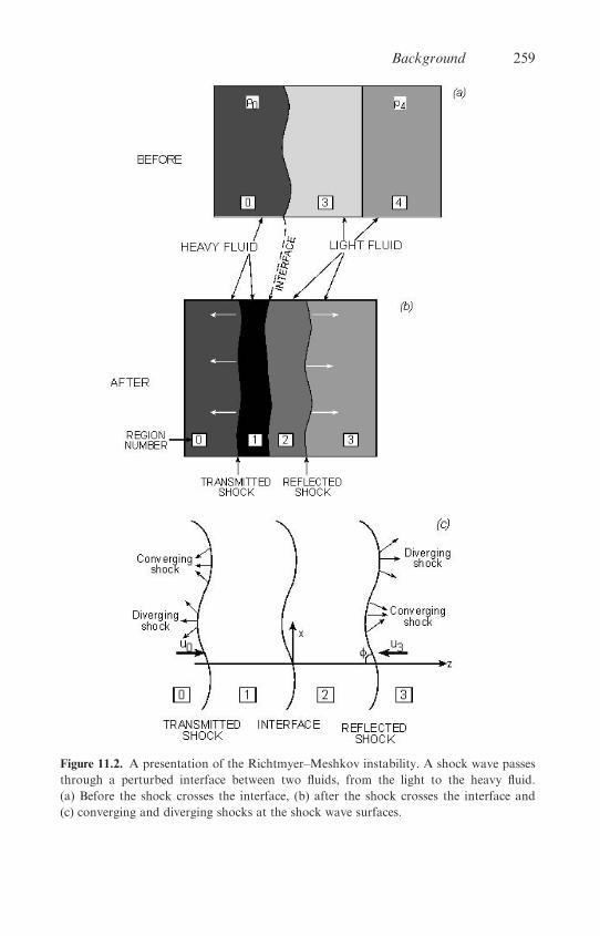
Figure 11.2. A presentation of the Richtmyer–Meshkov instability. A shock wave passes

through a perturbed interface between two fluids, from the light to the heavy fluid.

(a) Before the shock crosses the interface, (b) after the shock crosses the interface and

(c) converging and diverging shocks at the shock wave surfaces.

Background 259

In the following sections the RT, RM and KH instabilities are analysed.The RT instability is discussed in greater detail (the next four sections) thanthe other instabilities.

11.2 Rayleigh–Taylor Instability, Linear Analysis

The hydrodynamic equations describing the motion under consideration arethe following mass and the momentum conservation equations:

@�

@tþr � �vð Þ ¼ 0; �

@v

@tþ �ðv � rÞv ¼ �rPþ �g ð11:9Þ

where � is the fluid density, v is the flow velocity, P is the pressure and �g isthe external force acting on the fluid (if there is an acceleration, then a ¼ �g).The Cartesian coordinates with unit vectors xx, yy and zz are used, and thegravitational field (or the acceleration) is perpendicular to the interfacebetween the fluids

g ¼ �gzz: ð11:10Þ

The instability is investigated here in the linear approximation (Chandra-sekhar 1961, Hoffman 1995):

� ¼ �0 þ �1; �0 � �1

v ¼ v0 þ v1; v0 � v1

P ¼ P0 þ P1; P0 � P1:

ð11:11Þ

The variables with subscript 1 describe how a small perturbation grows intime. If the amplitude of the perturbation never returns to its initial value,then it is said that the flow is unstable with respect to the initial perturbation.Substituting (11.11) into equations (11.9), and neglecting higher orders thanone (see section 2.5), yields the following equations to the zeroth order andthe first order respectively:

@�0@t

þr � �0v0ð Þ ¼ 0; �0@v0@t

þ �0ðv0 � rÞv0 ¼ �rP0 þ �0g ð11:12Þ

@�1@t

þr � �0v1 þ �1v0ð Þ ¼ 0

�1@v0@t

þ �0@v1@t

þ �0 ðv1 � rÞv0 þ ðv0 � rÞv1½ � þ �1ðv0 � rÞv0 ¼ �rP1 þ �1g

ð11:13Þ

For the analysis of RT instability it is assumed that v0 ¼ 0, so that theequations (11.13) for the perturbations are simplified to

@�1@t

þr � �0v1ð Þ ¼ 0; �0@v1@t

þrP1 � �1g ¼ 0 : ð11:14Þ


For an incompressible fluid the speed of sound equals infinity, so thatcommunications by sound signal are instantaneous. Therefore, it is assumedthat an incompressible flow is a reasonable assumption for flow velocitiesmuch smaller than the local speed of sound. In Lagrangian coordinates(see section 3.2) the density in this case does not change with time:

d�

dt¼ @�

@tþ v � r� ¼ 0: ð11:15Þ

Using the linearization procedure in this equation, together with the first ofequations (11.14), one gets the following two equations:

r � v1 ¼ 0 ð11:16Þ

@�1@t

þ v1 � r�0 ¼ 0: ð11:17Þ

Instead of equations (11.14) we have to solve for the incompressible fluid thesecond equation of (11.14), together with equations (11.16) and (11.17). Inour problem �0 is constant in both fluids, and therefore the initial densitychanges only in the z direction, normal to the interface between the twofluids. This implies that @�0=@x ¼ 0, @�0=@y ¼ 0 and only at the interface@�0=@z 6¼ 0. Writing these equations explicitly in Cartesian coordinates,one gets

�0@v1x@t

þ @P1

@x¼ 0

�0@v1y@t

þ @P1

@y¼ 0

�0@v1z@t

þ @P1

@zþ �1g ¼ 0

@�1@t

þ v1z@�0@z

¼ 0

@v1x@x

þ@v1y@y

þ @v1z@z

¼ 0

ð11:18Þ

We have five equations with five unknowns, v1x, v1y, v1z, P1 and �1. It isconvenient to solve these equations after a Fourier transform in x–y, orequivalently the disturbance is analysed by its normal modes, with solutionsdepending on x, y and t in the following way:

v1 x; y; z; tð Þ ¼ uðzÞP1 x; y; z; tð Þ ¼ �PðzÞ�1 x; y; z; tð Þ ¼ ��ðzÞ

9>=>;� expðikxxþ ikyyþ �tÞ ð11:19Þ

Rayleigh–Taylor Instability, Linear Analysis 261

where kx, ky and � are constants. Substituting (11.19) into equations (11.18)gives

��0ux þ ikx�P ¼ 0

��0uy þ iky�P ¼ 0

��0uz þ@�P

@zþ g�� ¼ 0

uzd�0dz

þ �� ¼ 0

ikxux þ ikyuy þ@uz@z

¼ 0:

ð11:20Þ

Multiplying the first equation by ikx, the second equation by iky, adding thesetwo new equations and solving with the last equation, one gets

�PðzÞ ¼ ��0k2

�duzdz

ð11:21Þ

where k is defined by

k2 ¼ k2x þ k2y: ð11:22Þ

Substituting ��ðzÞ from the fourth equation of (11.20), together with �PðzÞfrom (11.21) into the third equation of (11.20), one gets the followingequation for uz:

d

dz

��0

duzdz

��k2�0 �

�k2g

�2

�d�0dz

�uz ¼ 0: ð11:23Þ

If the fluid is confined between two rigid planes at þzB and �zB, then theboundary conditions are

uzðzBÞ ¼ 0;

�duzdz

� zB

¼ 0: ð11:24Þ

We take in our following analysis zB ! 1. Equation (11.23) is an eigenvalueequation, with uz the eigenfunction and the term in [� � �] is the eigenvalue.Therefore, � is fixed for any given values of �0ðzÞ, k and g.

The interface is the surface z ¼ 0, and the density is assumed constantanywhere except between the fluids at z ¼ 0. Therefore, for z 6¼ 0, equation(11.23) is given by

z 6¼ 0:@2uzðzÞ@z2

� k2uzðzÞ ¼ 0 ð11:25Þ

and its general solution is

z 6¼ 0: uzðzÞ ¼ � expðkzÞ þ � expð�kzÞ: ð11:26Þ


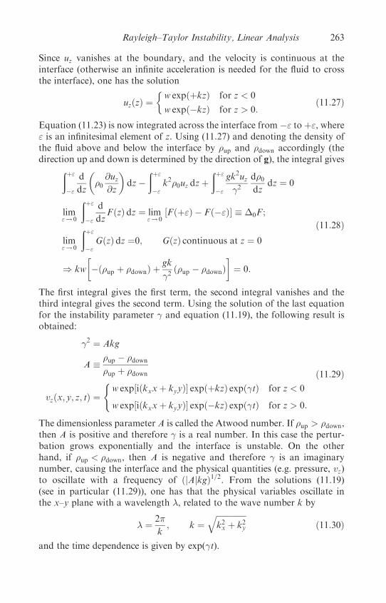
Since uz vanishes at the boundary, and the velocity is continuous at theinterface (otherwise an infinite acceleration is needed for the fluid to crossthe interface), one has the solution

uzðzÞ ¼�w expðþkzÞ for z < 0

w expð�kzÞ for z > 0:ð11:27Þ

Equation (11.23) is now integrated across the interface from �" toþ", where" is an infinitesimal element of z. Using (11.27) and denoting the density ofthe fluid above and below the interface by �up and �down accordingly (thedirection up and down is determined by the direction of g), the integral givesðþ"

�"

d

dz

��0@uz@z

�dz�

ðþ"�"

k2�0uz dzþðþ"�"

gk2uz�2

d�0dz

dz ¼ 0

lim"!0

ðþ"�"

d

dzFðzÞ dz ¼ lim

"!0½Fðþ"Þ � Fð�"Þ� � �0F ;

lim"!0

ðþ"�"

GðzÞ dz ¼0; GðzÞ continuous at z ¼ 0

) kw

��ð�up þ �downÞ þ

gk

�2ð�up � �downÞ

�¼ 0:

ð11:28Þ

The first integral gives the first term, the second integral vanishes and thethird integral gives the second term. Using the solution of the last equationfor the instability parameter � and equation (11.19), the following result isobtained:

�2 ¼ Akg

A ��up � �down�up þ �down

vzðx; y; z; tÞ ¼w exp½iðkxxþ kyyÞ� expðþkzÞ expð�tÞ for z < 0

w exp½iðkxxþ kyyÞ� expð�kzÞ expð�tÞ for z > 0:

( ð11:29Þ

The dimensionless parameter A is called the Atwood number. If �up > �down,then A is positive and therefore � is a real number. In this case the pertur-bation grows exponentially and the interface is unstable. On the otherhand, if �up < �down, then A is negative and therefore � is an imaginarynumber, causing the interface and the physical quantities (e.g. pressure, vz)to oscillate with a frequency of ðjAjkgÞ1=2. From the solutions (11.19)(see in particular (11.29)), one has that the physical variables oscillate inthe x–y plane with a wavelength �, related to the wave number k by

� ¼ 2�

k; k ¼

ffiffiffiffiffiffiffiffiffiffiffiffiffiffiffik2x þ k2y

qð11:30Þ

and the time dependence is given by exp(�t).

Rayleigh–Taylor Instability, Linear Analysis 263

11.3 Ablation-Surface Instability

The ablation-surface instability occurs when a laser is accelerating a solid foilor shell. In this case a high-pressure low-density plasma region is createdfrom the ablated material that accelerates the foil, due to the expandingplasma (the rocket effect). During the acceleration the foil is subject toRayleigh–Taylor instabilities since a low-density medium accelerates ahigh-density medium (for the high accelerations obtained here, the gravita-tion is not relevant).

Because energy is deposited at the interface between the foil (with adensity �foil) and the adjacent plasma (with a density �pl), a velocity dis-continuity is permitted at the interface together with the density jump. It isassumed that there is a sharp density jump, so that the density is describedby a function:

�0ðzÞ ¼ �plð�zÞ þ �foilðzÞ; ðzÞ ¼�1 for z > 0

0 for z < 0:ð11:31Þ

In the foil reference frame of coordinates (the foil is at rest in this frame), theablatedmaterial moves in the�zz direction (zz is a unit vector in the z direction)with velocity vpl:

v0 ¼ �vplð�zÞzz ¼��vplzz for z < 0

0 for z > 0:ð11:32Þ

The second equations of (11.12) and (11.13), without the gravitational term,can be combined in the following way:

�0

�@v1@t

þ v1 � rv0 þ v0 � rv1

�¼ �1�0

rP0 �rP1: ð11:33Þ

These three equations, together with the last two equations of (11.20) (theincompressibility assumption), are the five equations with the five unknownsto be solved. Substituting (11.19) into these equations leads, in a similar waythat equation (11.23) was obtained, to the following equation for the velocityuzðzÞ:

@

@z

��0@uz@z

�� k2�0v0z

�

@uz@z

��k2�0 �

ak2

�2@�0@z

þ k2�0�

@v0z@z

�uz ¼ 0 ð11:34Þ

where the acceleration a is defined by

a � ��1

�0

�@P0

@z: ð11:35Þ

Equation (11.34) is now integrated across the interface from �" toþ", where" is an infinitesimal element of z. The density and the initial velocity aredescribed by a function, and the derivative of these terms gives the Dirac


� function since

dðzÞdz

¼ �ðzÞ: ð11:36Þ

The integral of the Dirac function over the segment, including the zero of theargument, is equal to one, while the integral of regular functions and the function from �" to þ", where "! 0, is equal to zero. Therefore, theintegrals of the second and third terms of (11.34) vanish, the integrals ofthe first and fourth terms (using (11.27)) are similar to the integrals of(11.28), and only the integral of the fifth term in (11.34) is new and isequal toðþ"

�"

k2�0uz�

@v0z@z

dz ¼ k2w

�

ðþ"�"�0@v0z@z

dz ¼ k2w

�

��pl þ �foil

2

�vpl

�: ð11:37Þ

At the last step we have used the symmetry of � ð�ðzÞ ¼ �ð�zÞÞ and theidentity ðþ"

�"ðzÞ�ðzÞ dz ¼ 1

2ð11:38Þ

that can be easily verified from integrating by parts.Therefore, the integral of (11.34) over the interface yields (using (11.38)

and the integrals in (11.28))

kw

�ð�foil þ �plÞ �

ak

�2ð�foil � �plÞ þ

k

2�ð�foil þ �plÞvpl

�¼ 0: ð11:39Þ

Simplifying this equation gives

�2 þ�kvpl

2

�� akA ¼ 0; A �

�foil � �pl�foil þ �pl

: ð11:40Þ

The solution of this quadratic equation is

� ¼ �kvpl

4

ffiffiffiffiffiffiffiffiffiffiffiffiffiffiffiffiffiffiffiffiffiffiffiffiffiffiffiffiffiffiffi�kvpl

4

�2þ Aka

s

vpl 4

ffiffiffiffiffiffiAa

k

r) � �

ffiffiffiffiffiffiffiffiffiAka

p�kvpl

4þ � � � :

ð11:41Þ

From this result one can see that the ablation reduces (compare withequation (11.29) for g ¼ a) the growth rate of the RT instability.

In deriving equation (11.41), many simplifying assumptions have beenmade. For example, the incompressibility assumption, the spatial extentand the density gradient of the plasma were neglected, the plasma heatingwas not taken into account, etc.

It is interesting to point out that a detailed numerical simulation of theablation instability, taking all the above-mentioned effects into account

Ablation-Surface Instability 265

(Takabe et al. 1985) gives a fit described by equation (11.6). In comparisonbetween this fit and equation (11.41): there are two main differences theconstant 1

4 is changed to about 3 and ua is changed to vpl ððAÞ1=2 � 0:9 is agood approximation for the plasma–solid interface). While vpl is theplasma velocity far from the ablation surface, the ua represents the massablation rate per unit area divided by the density of the ablation surface.Since vpl � ua, the numerical fit (11.6) and equation (11.41) seem not to beinconsistent. There is, however, a difference between the numerical fit(11.6) and equation (11.41), since in the above value of � the approximationkvpl=4 ðAkaÞ1=2 has been made, while the numerical fit does not requirethis perturbation. Therefore, in analysing equation (11.6) it is permitted tointroduce a cutoff wavenumber kc, defined by

�ðkcÞ ¼ 0 ) kc ¼��

�

�2� a

u2a

�; �c �

2�

kc: ð11:42Þ

Equation (11.6) shows that for wavelength � < �c (i.e. k > kc) the ablation isstable, and only the wavelengths higher than �c contribute to the ablation RTinstability.

11.4 The Magnetic Field Effect

In high-power laser–plasma interactions very strong magnetic fields arecreated (see chapter 8). Megagauss magnetic fields (d.c.) were measured formoderate laser intensities. In this section it is shown that the magnetic fieldparallel to the accelerated interface between two fluids, where the heavierfluid is above the lighter fluid, stabilizes the RT instability.

The acceleration is assumed to be in the z direction, the interfacebetween the fluids are in the x–y plane z ¼ 0 and the fluids are incompressibleplasmas with zero resistivity (¼ 1/electrical conductivity¼ 1=E). The linear-ization procedure, as in equation (11.11), is used in this analysis with amagnetic field (Gaussian units are used):

B ¼ B0 þ B1; B0 ¼ const:;jB1jjB0j

1: ð11:43Þ

The momentum equation is (see equations (3.10) and (3.11), where theelectric field E is neglected relative to the B field)

�@v

@t¼ �rPþ 1

cðJ� BÞ ð11:44Þ

where v is the fluid velocity, � and P are density and pressure respectively, J isthe electric current and c is the speed of light. Using the Maxwell equation,

J ¼�

c

4�

�r� B: ð11:45Þ


The linearized momentum equation can be written

�0@v

@t¼ �rP1 �

B0

4�� ðr � B1Þ � g�1zz: ð11:46Þ

This equation has to be solved, together with the following linearizedMaxwell equation for zero resistivity (see equation (8.33), with 1=E ¼ 0):

@B

@t¼ �cr� E ¼ r� ðv� B0Þ ð11:47Þ

the mass conservation and the incompressibility requirement (equations(11.16) and (11.17)). In these approximations, the zero divergence of themagnetic field

r � B1 ¼ 0 ð11:48Þ

is not an independent equation, since it is derived from equation (11.47).In this problem there are eight independent equations, (11.46), (11.47),

(11.16) and (11.17), with eight unknowns, �1, P1, v and B1. We shall writeexplicitly these equations for two cases:

1. The initial magnetic field is perpendicular (vertical) to the interfacebetween the fluids, B0 ¼ B0zz.

2. The initial magnetic field is parallel (horizontal) to the interface betweenthe fluids, B0 ¼ B0xx:

B0 ¼ B0zz: �0@vx@t

¼ � @P1

@xþ B0

4�

�@B1x

@z� @B1z

@x

�

�0@vy@t

¼ � @P1

@yþ B0

4�

�@B1y

@z� @B1z

@y

�

�0@vz@t

¼ � @P1

@z� g�1

@B1

@t¼ B0

@v

@z; r � v ¼ 0;

@�1@t

þ vz@�0@z

¼ 0

ð11:49Þ

B0 ¼ B0xx: �0@vx@t

¼ � @P1

@x

�0@vy@t

¼ � @P1

@yþ B0

4�

�@B1y

@x� @B1x

@y

�

�0@vz@t

¼ � @P1

@zþ B0

4�

�@B1z

@x� @B1x

@z

�� g�1

@B1

@t¼ B0

@v

@x; r � v ¼ 0;

@�1@t

þ vz@�0@z

¼ 0:

ð11:50Þ

The Magnetic Field Effect 267

As in the previous two sections, the following x–y–t dependence of thevariables is assumed:

v ¼ uðzÞB1 ¼ �BðzÞP1 ¼ �PðzÞ�1 ¼ ��ðzÞ

9>>>>=>>>>;

� expðikx þ iky þ �tÞ: ð11:51Þ

Substituting (11.51) into equations (11.49) and (11.50) yields, after algebraicmanipulations, the following differential equations for the two cases underconsideration:

B ¼ B0zz:�d

dz

��0

d

dz

�� B2

0

4��2

�d2

dz2� k2

�d2

dz2

�uzðzÞ ¼

��0k

2 � gk2

�2

�d�0dz

��uzðzÞ:

ð11:52Þ

B ¼ B0xx:�d

dz

��0

d

dz

�þ B2

0k2x

4��2

�d2

dz2� k2

��uzðzÞ ¼

��0k

2 � gk2

�2

�d�0dz

��uzðzÞ:

ð11:53Þ

In laser–plasma interaction the horizontal magnetic field might play animportant role in stabilizing the RT instabilities. In particular, if the larged.c. magnetic field (e.g. the vector product of the density gradient and thetemperature gradient; see chapter 8), created in the corona, penetratesinto the ablation surface then the ablation surface instability is significantlymodified. Therefore, only equation (11.53) is further analysed in the follow-ing part of this section.

For kx ¼ 0, equation (11.53) is identical to equation (11.23), where nomagnetic field is applied. Therefore, the disturbances that are independentof the coordinate along the direction of B0 (perpendicular to g) are notaffected by the existence of the magnetic field. In this case, B0 does notcontribute to the development of the RT instability. In other words, themagnetic field in the x direction, which can stabilize the RT instabilitiesfor wavelengths shorter than a critical value �c, does not stabilize any RTinstability that develops along the y direction.

For kx 6¼ 0. the RT instabilities in the hydromagnetic problem (equation(11.53)) are not identical to the RT instabilities in the hydrodynamic problem(equation (11.23)). We solve equation (11.53) for two uniform fluidsseparated at the surface z ¼ 0, with a density distribution given by

�ðzÞ ¼ �upðzÞ þ �downð�zÞ: ð11:54Þ


At the horizontal boundary z ¼ 0, the following continuity conditions mustbe satisfied:

lim"!0

fuzðþ"Þ ¼ uzð�"Þg

lim"!0

fBzðþ"Þ ¼ Bzð�"Þg:ð11:55Þ

The second equation follows from the first equation (or vice versa) by the useof (11.51) in the fourth equation of (11.50). The physical meaning of the firstequation (11.55) is that there is not an infinite acceleration when a fluidelement crosses the interface, while the second equation describes the factthat monopoles do not exist (r � B ¼ 0). Using the solution (11.27), whichis also valid in this problem, one gets by integrating equation (11.53) alongthe interface (similar to the integrals in the previous two sections):

�2 ¼ gk

��up � �down�up þ �down

� B20k

2x

2�ð�up þ �downÞgk

�: ð11:56Þ

The angle � between the k vector and the initial magnetic field (x axis), andthe wavelength of a sinusoidal disturbance (a normal mode), are defined by

cos� ¼ kxk

¼ kxffiffiffiffiffiffiffiffiffiffiffiffiffiffiffik2x þ k2y

q ; � ¼ 2�

k : ð11:57Þ

The stable modes, �2 < 0, are therefore satisfying

� <B20 cos

2 �

g�� c; �� up � �down : ð11:58Þ

For example, in laser plasma acceleration with g � 1015 cm/s2, magneticfields of the order of 10MG, �� 1 g/cm3 and cos� � 0:5, one gets stablemodes for wavelengths smaller than 0.05 cm, a non-negligible dimensionfor high-intensity laser–plasma interactions.

It is interesting to see that if cos�! 0, then the hydromagnetic result(11.56) goes to the hydrodynamic result (11.29).

We end this section by pointing out that surface tension st (dimensionerg/cm2 ¼ dyne/cm) also stabilizes the RT instability (Chandrasekhar 1961).The hydrodynamic instability in this case gives a similar result to equation(11.56) with the substitution

st !B20 cos

2 �

2�k; �2 ¼ gk

��up � �down�up þ �down

� k2stgð�up þ �downÞ

�: ð11:59Þ

11.5 Bubbles from Rayleigh–Taylor Instability

It has been shown in section 11.2 that the amplitude of a sinusoidal per-turbation increases exponentially with time in the RT instability. When the

Bubbles from Rayleigh–Taylor Instability 269

amplitude becomes of the order of the wavelength (>0:1�), then higherharmonics of the original perturbation appear in the disturbance. The inter-action between the different modes results in the formation of bubbles, withthe light fluid penetrating into the heavy fluid and spikes of heavy fluid fallinginto the light fluid. The full-time development of the RT instability has beendiscussed in the literature (Davies and Taylor 1950, Layzer 1955). In thissection the asymptotic steady state of the bubble motion is considered(Hoffman 1995) using the potential flow theory.

For an incompressible irrotational fluid the flow velocity vðr; tÞ satisfiesthe following equations:

r � v ¼ 0; r� v ¼ 0 ð11:60ÞUsing these equations and the identity r� ðr’Þ ¼ 0, one can define avelocity potential � which obeys the Laplace equation:

r2’ ¼ 0: ð11:61ÞThe Cartesian coordinates are chosen in such a way that the bubble moves inthe z direction and the vector k (kx ¼ k, ky ¼ 0) is chosen in the x direction sothat the y direction can be neglected. The bubble surface motion is analysedin the bubble centre of mass coordinates, where the Laplace equation takesthe form

@2’

@x2þ @2’

@z2¼ 0: ð11:62Þ

The following boundary conditions are appropriate for this problem:

vx

�x ¼ �

2

�¼ 0; vzðz ¼ þ1Þ ¼ �u : ð11:63Þ

The first equation describes an array of identical moving bubbles with aperiod of � ¼ 2�=k, or equivalently one bubble with a radius � movingbetween two parallel frictionless walls at x ¼ �=2. The second boundarycondition is equivalent to the motion of a bubble with an asymptoticconstant velocity u, or equivalently in the frame of reference of the bubblethe flow is moving at z ¼ infinity with a velocity �u.

The solution of equation (11.62), subject to the boundary conditions(11.63), is

’ðx; zÞ ¼ �zu� �

2�

X1n¼1

�ann

�exp

�� 2�nz

�

�cos

�2�nx

�

�

vx ¼ @’

@x; vy ¼

@’

@y:

ð11:64Þ

It is convenient at this stage to introduce the concept of streamlines (Courantand Friedrichs 1948, Landau and Lifshitz 1987). The tangent to a streamlineat any point on this line gives the direction of the velocity at that point as


determined by the differential equations dx=vx ¼ dy=vy ¼ dz=vz. In steadyflow the streamlines are constant in time and coincide with the trajectoriesof the fluid particles. In this case a particle trajectory is given by a constantvalue of the stream function , associated with the velocity potential by

@

@x¼ @’

@z;

@

@z¼ � @’

@x: ð11:65Þ

The stream function that satisfies equations (11.64) and (11.65) is given by

ðx; zÞ ¼ �xu� �

2�

X1n¼1

�ann

�exp

�� 2�nz

�

�sin

�2�nx

�

�: ð11:66Þ

At z ¼ þ1 the stream function equals �xu. Since in this model all thebubbles are identical, it is convenient to choose a trajectory

ðx; zÞ ¼ 0: ð11:67ÞSubstituting (11.67) into (11.66) yields the equation that describes the surfaceof a bubble:

1 ¼ �

2�xu

X1n¼1

�ann

�exp

�� 2�nz

�

�sin

�2�nx

�

�: ð11:68Þ

This equation has been solved (Davies and Taylor 1950) by using only thefirst term in the potential and in the streaming functions, i.e. an 6¼ 0 onlyfor n ¼ 1. Under this assumption the fluid flow velocity is

vx ¼ a1 exp

�� 2�z

�

�sin

�2�x

�

�

vz ¼ �uþ a1 exp

�� 2�z

�

�cos

�2�x

�

� ð11:69Þ

and the surface of the bubble is described by

a1 exp

�� 2�z

�

�sin

�2�x

�

�¼ 2�xu

�: ð11:70Þ

Choosing the coordinates in such a way that for x ¼ 0 the peak of the bubbleis at z ¼ 0, then one has to solve equations (11.69) and (11.70) for

a1 ¼ u ð11:71Þin order to find the asymptotic velocity u.

For a steady flow ð@v=@t ¼ 0), like the case under consideration, themomentum equation yields the famous Bernoulli law along a streamline:

1

2v2 þ P

�þ gz ¼ const: ð11:72Þ

In the present model it is assumed that the Atwood number A � 1, i.e. theupper fluid has a density much larger than the lower fluid. Therefore, it is

Bubbles from Rayleigh–Taylor Instability 271

conceivable to assume a constant pressure within the lower density bubble atits border with the heavy fluid. On the other hand, the high-density fluid is inequilibrium with the bubble, and combining this with the assumption ofconstant density (incompressible fluid), one can rewrite Bernoulli’s equation:

0 ¼ 12 ðv

2x þ v2yÞ þ gz ð11:73Þ

where the constant has been taken at zero since the peak at z ¼ 0 of thebubble is a stagnation point with vx ¼ vy ¼ 0. Substituting (11.69) and(11.71), into (11.73) one gets

1þ exp

�� 4�z

�

�� 2 exp

�� 2�z

�

�cos

�2�x

�

�þ 2gz

u2¼ 0: ð11:74Þ

One has to solve the momentum equation, as expressed in equation (11.74),together with the bubble surface equation (11.70) (with a1 ¼ u), yielding thefollowing equation for x:

�2 tan � � 2� sin2 � þ tan � sin2 � þ�g�

�u2

�tan � sin2 � ln

�sin �

�

�¼ 0

� � 2�x

�:

ð11:75Þ

Except for � ¼ 0 (i.e. x ¼ 0), this equation has only one solution for a givenvalue of g�=u2. In order to get the more general solution for all points onthe bubble surface, one has to take into account the full expansions (ormore terms) of equations (11.64) and (11.68). However, u can be obtainedto a good approximation by solving equation (11.75) in the neighbourhoodof x ¼ 0 for different values of g, � and u. For this purpose this equation isexpanded in a series of �, yielding the following equation to the lowest relevantorder (�5):

�5�1� g�

6�u2

�¼ 0 ð11:76Þ

with the following solution, for the asymptotic velocity of the bubble:

u ¼ffiffiffiffiffiffig�

6�

r� 0:2304

ffiffiffiffiffiffig�

p: ð11:77Þ

As explained in section 11.1, equations (11.2), (11.3) and (11.4), this result isconsistent with balancing the buoyancy force and the drag force acting on arising bubble.

11.6 Richtmyer–Meshkov Instability

The Richtmyer–Meshkov (RM) instability is named after Robert D.Richtmyer, who suggested and also developed the theory of the instability,


and E. E. Meshkov, who proved experimentally the existence of this insta-bility. The RM instability describes the behaviour of the interface betweentwo fluids or gases, traversed by a shock wave. This interface is unstablewhen the shock wave crosses from the lighter to the heavier media and it isalso unstable when the shock wave passes in the opposite direction. Aschematic presentation of RM instability is given in figure 11.2. The shockwave imparts an impulsive acceleration to the interface, and as a result aninterface disturbance grows initially linearly with time, it saturates, and itcan develop into bubbles and spikes like in the RT instability.

We analyse two incompressible fluids with a disturbance of the interfacegiven by

zðx; tÞ ¼ �ðtÞ expðikxÞ; k� 1 ð11:78Þ

where the real part of the right-hand side (i.e. cos kx) is taken to describe thereal z values. If the system is accelerated in the z direction with an accelera-tion gðtÞ, then the amplitude of the interface disturbance satisfies theequation:

d2�ðtÞdt2

¼ kgðtÞA�ðtÞ; A ��up � �down�up þ �down

: ð11:79Þ

This equation is easily obtained from equations (11.29) in the two-dimensionalspace x–z. The fluid flow velocity solution derived in (11.29) satisfies

@2vz@t2

¼ �2vz; �2 ¼ kgA ð11:80Þ

and therefore, if the displacement �ðtÞ is defined by

@�

@t¼ vz ð11:81Þ

then equation (11.80) implies the validity of equation (11.79).Denoting byU the increment of the velocity of an instantaneous impulse

at t ¼ 0,

gðtÞ ¼ U �ðtÞ )ðgðtÞ dt ¼ U ð11:82Þ

where �ðtÞ is the Dirac delta function, then equation (11.79) can be integratedto give

before impulse ðt < 0Þ: � ¼ �0;d�

dt¼ 0

immediately after impulse: � ¼ �0;d�

dt¼ kUA�0:

ð11:83Þ

As can be seen from this equation, after the impulse the amplitude � grows ata constant rate.

Richtmyer–Meshkov Instability 273

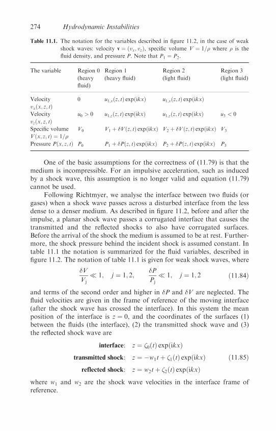
One of the basic assumptions for the correctness of (11.79) is that themedium is incompressible. For an impulsive acceleration, such as inducedby a shock wave, this assumption is no longer valid and equation (11.79)cannot be used.

Following Richtmyer, we analyse the interface between two fluids (orgases) when a shock wave passes across a disturbed interface from the lessdense to a denser medium. As described in figure 11.2, before and after theimpulse, a planar shock wave passes a corrugated interface that causes thetransmitted and the reflected shocks to also have corrugated surfaces.Before the arrival of the shock the medium is assumed to be at rest. Further-more, the shock pressure behind the incident shock is assumed constant. Intable 11.1 the notation is summarized for the fluid variables, described infigure 11.2. The notation of table 11.1 is given for weak shock waves, where

�V

Vj

1; j ¼ 1; 2;�P

Pj

1; j ¼ 1; 2 ð11:84Þ

and terms of the second order and higher in �P and �V are neglected. Thefluid velocities are given in the frame of reference of the moving interface(after the shock wave has crossed the interface). In this system the meanposition of the interface is z ¼ 0, and the coordinates of the surfaces (1)between the fluids (the interface), (2) the transmitted shock wave and (3)the reflected shock wave are

interface: z ¼ �0ðtÞ expðikxÞ

transmitted shock: z ¼ �w1tþ �1ðtÞ expðikxÞ

reflected shock: z ¼ w2tþ �2ðtÞ expðikxÞ

ð11:85Þ

where w1 and w2 are the shock wave velocities in the interface frame ofreference.

Table 11.1. The notation for the variables described in figure 11.2, in the case of weak

shock waves: velocity v ¼ ðvx; vzÞ, specific volume V ¼ 1=� where � is the

fluid density, and pressure P. Note that P1 ¼ P2.

The variable Region 0

(heavy

fluid)

Region 1

(heavy fluid)

Region 2

(light fluid)

Region 3

(light fluid)

Velocity

vxðx; z; tÞ0 u1;xðz; tÞ expðikxÞ u1;xðz; tÞ expðikxÞ

Velocity

vzðx; z; tÞu0 > 0 u1;zðz; tÞ expðikxÞ u1;zðz; tÞ expðikxÞ u3 < 0

Specific volume

Vðx; z; tÞ ¼ 1=�

V0 V1 þ �Vðz; tÞ expðikxÞ V2 þ �Vðz; tÞ expðikxÞ V3

Pressure Pðx; z; tÞ P0 P1 þ �Pðz; tÞ expðikxÞ P2 þ �Pðz; tÞ expðikxÞ P3


Since we are using the linear theory, one can take exp(ikx) and�i exp(ikx) for cos kx and sin kx respectively. In general, complex functionsare used with the meaning that at the last step the real values should be taken.

11.6.1 The differential equation for the pressure in regions 1 and 2

This analysis is a first-order perturbation theory with the small variables asgiven by (11.84) and also u1;z w1 and w2, and �jk (for j ¼ 0; 1; 2) 1.For a weak shock wave (Zeldovich and Raizer 1966), the first-order perturba-tion theory gives the following relation between the pressure increase �P andthe specific volume change �V (note that the notation of table 11.1 is used):

�Pðz; tÞ ¼�@P

@V

�S

�Vðz; tÞ ¼ ��c21V2

1

��Vðz; tÞ ð11:86Þ

where c1 is the speed of sound in the undisturbed medium of region 1 (theheavy fluid). This equation can be considered as the equation of state inour approximation.

The mass conservation, the first of equations (11.14), can be written as

@

@t

�1

V1 þ �V

�þ�

1

V1 þ �V

�r � vðx; z; tÞ ¼ 0

) V1

�iku1;x þ

@u1;z@z

�¼ @ð�VÞ

@t¼ �

�V2

1

c21

�@ð�PÞ@t

ð11:87Þ

where at the last step equation (11.86) has been used.The following two equations are obtained from the momentum con-

servation:�1

V1 þ �V

�@vðx; z; tÞ

@t¼ �r½P1 þ �Pðz; tÞ expðikxÞ�

)

1

V1

@u1;z@t

¼ � @ð�PÞ@z

1

V1

@u1;x@t

¼ �ik�P:

8>>><>>>:

ð11:88Þ

From equations (11.87) (one equation) and (11.88) (two equations), thefollowing wave equation is derived for �Pðz; tÞ in region 1 (see figure 11.2),and similarly the second wave equation is obtained in region 2 with thesubstitution c1 ! c2:

@2

@t2ð�PÞ � c21

�@2

@z2� k2

�ð�PÞ ¼ 0

@2

@t2ð�PÞ � c22

�@2

@z2� k2

�ð�PÞ ¼ 0:

ð11:89Þ


11.6.2 The boundary conditions on the interface

In order to solve equations (11.89) in regions 1 and 2, the equations at theboundaries of these domains have to be defined. Region 1 is defined betweenthe interface (between the fluids) and the transmitted shock surfaces, whileregion 2 is between the interface and the reflected shock. The normal fluidvelocities from both regions are equal at the interface, and therefore one canalso write the acceleration continuity on the interface. Using the interfaceequation (11.85) and the momentum equation (11.88), the following boundaryequations are derived by the requirement that the accelerations in thez direction, @u1;z=@t and @u2;z=@t are continuous:

d2�0ðtÞdt2

¼��V1

�@ð�PÞ@z

��z¼�0�

V1

�@ð�PÞ@z

��z¼�0

¼�V2

�@ð�PÞ@z

��z¼þ0

:

ð11:90Þ

The second equation is the needed boundary (at the interface) for the partialdifferential equation (11.89). The main objective of this problem is the studyof the RM instability, and for this purpose the first of equations (11.90) givesthe required information, i.e. the calculation of �0(t).

In order to complete this problem the boundary conditions at the shock-wave surfaces are also needed.

11.6.3 The boundary conditions at the shock-wave surfaces

First, we use the Hugoniot relations (equations (10.36)) on the boundary ofregions 2 and 3, at the reflected shock wave. One has to note that the initialconditions for the Hugoniot equations are those obtained at the final stageafter the crossing of the first shock wave. In other words, the reflectedshock enters a shocked medium. Moreover, area 3 has also been shockedbefore the present analysis is considered. However, for this domain thesimple Hugoniot relations can be used, and P3 and V3 are easily calculatedfrom the initial conditions of region 4, as shown in figure 11.2(a).

Therefore, the first and the fourth equations of (10.36) on the boundaryof regions 2 and 3 can be written in the following way:

w2 þ _��2ðtÞ expðikxÞ � u1;zðw2t; tÞ expðikxÞV2 þ �Vðw2t; tÞ expðikxÞ

¼ w2 þ _��2ðtÞ expðikxÞ � u3V3

w2 þ _��2ðtÞ expðikxÞ � u3V3

¼

ffiffiffiffiffiffiffiffiffiffiffiffiffiffiffiffiffiffiffiffiffiffiffiffiffiffiffiffiffiffiffiffiffiffiffiffiffiffiffiffiffiffiffiffiffiffiffiffiffiffiffiffiffiffiffiffiffiffiffiffiffiP2 þ �Pðw2t; tÞ expðikxÞ � P3

V3 � V2 � �Vðw2t; tÞ expðikxÞ

sð11:91Þ


where the dot means time derivative and P2 = P1. The Hugoniot relationsin the form of equations (10.36) are correct only for the velocity compo-nents perpendicular to the shock surface. Since the shock front is not aplane, one has to multiply the fluid velocities in these equations with thecosines of the angle between the velocity and the normal to the surface.However, since the angles are first-order variables, these cosines differfrom unity by second-order quantities. Therefore, equations (11.91) arecorrect only to first order in perturbation theory, and by expanding theseequations the following zeroth- and first-order equations are obtainedrespectively:

w2

V2

¼ w2 � u3V3

;w2

V2

¼ffiffiffiffiffiffiffiffiffiffiffiffiffiffiffiffiffiP2 � P3

V3 � V2

sðnote:P 2 ¼ P1Þ ð11:92Þ

1

V2

�d�2dt

� u1;zðw2t; tÞ�� w2

V22

�Vðw2t; tÞ

¼ 1

2


V3 � V2

s ��Pðw2t; tÞP2 � P3

þ �Vðw2t; tÞV3 � V2

�

1

V3

d�2dt

¼ 1

2


V3 � V2

s ��Pðw2t; tÞP2 � P3

þ �Vðw2t; tÞV3 � V2

�:

ð11:93Þ

Inspecting the zeroth-order equations (11.92), one can easily recognize theHugoniot jump conditions for planar one-dimensional waves. It turns outthat our problem to zeroth order can be described by planar waves. Thecorrugation of the surfaces (interface and the shock waves) are describedin this analysis by the first-order terms. Using the property that the Hugoniotpressure derivative with respect to the specific volume equals the isentropederivative at the initial point on the Hugoniot (equation (10.99)), the first-order expansion of the Hugoniot pressure can be described by

�Pðw2t; tÞ � �P2ðtÞ ¼�d�P2

dV

�V2

�V ¼�dPS

dV

�V2

�V

¼ � c22�V

ðV2 þ �VÞ2� c22�V

V22

ð11:94Þ

where PS is the isentropic pressure. Substituting this result into the secondequation of (11.93) yields the following boundary condition:

d�2ðtÞdt

¼ 1

2

�V3V2

V3 � V2

��c22 � w2

2

c22w2

��P2ðtÞ

�P2ðtÞ � �Pðz ¼ w2t; tÞ:ð11:95Þ


A similar procedure at the transmitted shock-wave surface yields a similarboundary relation:

d�1ðtÞdt

¼ 1

2

�V0V1

V0 � V1

��c21 � w2

1

c21w1

��P1ðtÞ

�P1ðtÞ � �Pðz ¼ �w1t; tÞ:ð11:96Þ

A second boundary value equation for the reflected shock-wave surface isobtained by the use of the first equation of (11.93). Substituting into this equa-tion the relation between �P and �V at the shock front (equation (11.94)), andcomparing the obtained value of d�2=dt with that derived in (11.95), gives

u1;zðw2t; tÞ ¼1

2V2

�c22 þ w2

2

c22w2

��P2ðtÞ: ð11:97Þ

By multiplying both sides of this equation with the total derivative, anddescribing the change in time of a moving fluid element on the shock surface,one gets�@

@tþ w2

@

@z

�u1;zðz ¼ w2t; tÞ ¼

1

2V2

�c22 þ w2

2

c22w2

��@

@tþ w2

@

@z

��Pðz ¼ w2t; tÞ:

ð11:98Þ

At this stage the mass and momentum equations (equations (11.87) and(11.88)) are necessary. However, before using these equations one has tocalculate the x derivative of u1;x.

The component of the fluid velocity v, parallel to the shock surface, iscontinuous across this surface. Therefore, one can write to the first order inour perturbation theory (see figure 11.2(c)) (note u1;x ¼ u2;x and u1;z ¼ u2;z):

u1;xðw2t; tÞ expðikxÞ ¼ u3 tan�

tan� ¼ @z

@x¼ @

@x½w2tþ �2ðtÞ expðikxÞ� ¼ ik�2ðtÞ expðikxÞ

) ikw2u1;xðz ¼ w2t; tÞ ¼ �k2w2u3�2ðtÞ:

ð11:99Þ

Adding this result to equation (11.98) and using the following mass andmomentum equations for region 2 (similar to equations (11.87) and (11.88)):

@u1;z@z

þ iku1;x ¼ �V2

c22

@�P

@t; �ik�P ¼ 1

V2

@u1;x@t

ð11:100Þ

one gets the following second boundary condition on the surface of thereflected shock wave:�

3

2w2 þ

c222w2

�d

dtð�P2Þ ¼ ðw2

2 � c22Þ@

@z½�Pðz ¼ w2t; tÞ� þ

k2c22w2u3V2

�2ðtÞ:

ð11:101Þ


A similar second boundary condition is given for the transmitted shock-wavesurface:�3

2w1 þ

c212w1

�d

dtð�P1Þ ¼ � ðw2

1 � c21Þ@

@z½�Pðz ¼ �w1t; tÞ� þ

k2c21w1u0V1

�1ðtÞ:

ð11:102ÞThe boundary conditions given in equations (11.101) and (11.102) describethe change in time of the shock-wave pressures. The first term on the right-hand side of these equations is the pressure gradient contribution behindthe shock. The second term on the right-hand side of these equationsdescribes the convergence or divergence of the shock-wave propagationdue to the corrugation of the shock surfaces (see figure 11.2(c)).

In this analysis of the RM instability, we have discussed only the lineardevelopment of the flow using weak shock waves. The differential equations(11.89) are subject to the boundary equations described by equations (11.90),(11.95), (11.96), (11.101) and (11.102). It is evident that a proper solutionof this problem requires the help of a computer. However, the solution of thecomplete nonlinear problem describing the full development of the RMinstability needs two- and three-dimensional sophisticated numerical analysis.

11.7 Kelvin–Helmholtz Instability

The Kelvin–Helmholtz (KH) instability occurs (Kelvin (1910), Helmholtz(1881)) when two different layers of fluids are in relative motion, such asthe generation of water waves by wind blowing over the surface of thewater (see figure 11.3).

In laser–plasma interactions the KH instability may occur during the laterstages of RT and RM instabilities, during the motion of the bubbles and thespikes. For example, the low-density bubbles move relative to the heavyfluid background with appropriate conditions to create KH instabilities.

The motion of an incompressible, inviscid (no viscosity) fluid streamingin the horizontal direction is now considered. The surface tension is neglectedin this analysis, although it is straightforward to include this stabilizing effect.It is assumed that the streaming takes place in the x direction with a velocityU, where U is an arbitrary function of z. The fluid is accelerated in thez direction, or equivalently it moves in a potential described by the accelera-tion g (in the �z direction). First-order perturbation is assumed with thefollowing notation (see equation (11.11)):

1. The flow velocity is vðx; y; z; tÞ þUðzÞxx, where the velocity componentsof v ¼ ðvx; vy; vzÞ are first-order terms ðv0 ¼ 0 and v1 is denoted here by v).

2. The fluid density is �ðx; y; z; tÞ ¼ �0ðzÞ þ �1ðx; y; z; tÞ, where �1 is a first-order term.

Kelvin–Helmholtz Instability 279

3. The pressure is P ¼ P0 þ P1ðx; y; z; tÞ, with P1 a first-order term.

The momentum conservation, mass conservation and the incompressiblefluid assumption give five equations similar to those in (11.18). The followingequations are derived by substituting v by vþU in the conservationequations (11.9) and using a similar first-order perturbation theory, as hasbeen done for example in section 11.2:

�0@vx@t

þ �0U@vx@x

þ �0vzdU

dzþ @P1

@x¼ 0

�0@vy@t

þ �0U@vy@x

þ @P1

@y¼ 0

�0@vz@t

þ �0U@vz@x

þ @P1

@zþ g�1 ¼ 0

@�1@t

þU@�1@x

þ vzd�0dz

¼ 0

@vx@x

þ@vy@y

þ @vz@z

¼ 0:

ð11:103Þ

We assume that the interface between the fluids is initially at z ¼ 0, thedisturbance �ðx; y; tÞ is in the z direction (also a first order perturbationterm) and it obeys the following equation:

@�

@tþUðz ¼ �Þ @�

@x¼ vzðz ¼ �Þ: ð11:104Þ

Figure 11.3. Two fluids A and B, with densities �A and �B, moving with different horizon-

tal velocities UA andUB. The interface between the two media develops a disturbance with

a wave number k ¼ 2�=�.


This equation describes the velocity of the disturbance normal to the interface.Analysing the disturbance by its normal modes, one can look for the followingsolutions (note that here the time dependence is exp(i�t), while in (11.19) it isexp(�t)):

vðx; y; z; tÞ ¼ uðzÞ�1ðx; y; z; tÞ ¼ ��ðzÞP1ðx; y; z; tÞ ¼ �PðzÞ�ðx; y; tÞ ¼ �0

9>>>>=>>>>;

� exp½iðkxxþ kyyþ �tÞ�: ð11:105Þ

Substituting (11.105) into equations (11.103) and (11.104), one gets accordingly

i�0ð�þ kxUÞux þ �0

�dU

dz

�uz þ ikx�P ¼ 0

i�0ð�þ kxUÞuy þ iky�P ¼ 0

i�0ð�þ kxUÞuz þ�d�P

dz

�þ g�� ¼ 0

ið�þ kxUÞ��þ uz

�d�0dz

�¼ 0

iðkxxþ kyyÞ þ�duzdz

�¼ 0

ð11:106Þ

ið�þ kxU�Þ�0 ¼ u�; U� � Uðz ¼ �Þ; u� � uðz ¼ �Þ: ð11:107Þ

Similar to the algebra used to solve equations (11.20), the following differen-tial equation is obtained for uzðzÞ by solving equations (11.106):

d

dz

��0ð�þ kxUÞ d

dz

��0kx

�dU

dz

��uzðzÞ

¼�k2�0ð�þ kxUÞ þ gk2

ð�þ kxUÞ

�d�0dz

��uzðzÞ: ð11:108Þ

This differential equation is subject to boundary conditions such as thatgiven in (11.24). Furthermore, from equation (11.107) it follows that

uzðz ¼ � þ 0Þ�þ kxUðz ¼ � þ 0Þ ¼

uzðz ¼ � � 0Þ�þ kxUðz ¼ � � 0Þ ð11:109Þ

i.e. if one approaches the interface from below or from above, the same valueof �0 is obtained, or in other words, ifU is continuous at the interface then uzis also continuous there; however, if U is discontinuous, then the normaldisplacement on the interface at any point on the surface should be uniquelydefined.

At this stage the ‘jump’ condition on the interface between the fluids isdefined. For this purpose one has to integrate equation (11.108) across the


interface from � � " to � þ " in the limit that " goes to zero. As in (11.28), wedefine

lim"!0

ð�þ "�� "

d

dzFðzÞ dz ¼ lim

"!0½Fð� þ "Þ � Fð� � "Þ� � ��F

lim"!0

ð�þ "�� "

GðzÞ dz ¼ 0; GðzÞ continuous at z ¼ �

lim"!0

ð�þ "�� "

�ðz� �Þ dz ¼1:

ð11:110Þ

Integrating (11.108) and using (11.109) and (11.110), the following boundarycondition (or as occasionally it is called, ‘the jump’ equation) is satisfied atthe interface between the fluids:

��

��0ð�þ kxUÞ duz

dz� �0kx

�dU

dz

�uz

�¼ gk2

�uz

�þ kxU

�z¼ �

��0: ð11:111Þ

We calculate explicitly this equation for the following problem. Two uniformfluids, separated at the surface z ¼ 0, have densities �A and �B (see figure11.3). The upper fluid has a density �A smaller than the lower fluid �B, sothat in this case we do not analyse the RT instability. Regarding the stream-ing, it is assumed that the upper fluid and the lower fluid stream haveconstant velocities UA and UB respectively.

Equation (11.108) for constant �0 and U, i.e. anywhere except at theinterface between the fluids, reduces to

�d2

dz2� k2

�uzðzÞ ¼ 0: ð11:112Þ

The general solution of this equation is a linear combination of exp(kz)and exp(�kz). Taking into account that uz vanishes at 1, and at z ¼ 0equation (11.109) must be satisfied, one obtains the solution

uzðzÞ ¼wð�þ kxUBÞ expðkzÞ for z < 0

wð�þ kxUAÞ expð�kzÞ for z > 0:

(ð11:113Þ

Using (11.110), the jump relations relevant for this problem are

�0

��0ð�þ kxUÞ duz

dz

�¼ kw½�Að�þ kxUAÞ2 þ �Bð�þ kxUBÞ2�

�0

��0kx

�dU

dz

�uz

�¼ 0

gk2�

uz�þ kxU

��0ð�0Þ ¼ wgk2ð�A � �BÞ:

ð11:114Þ


Substituting (11.114) into (11.111) yields the following quadratic equationin �:

�2 þ 2kx�A þ �B

ð�AUA þ �BUBÞ�

þ�

k2x�A þ �B

ð�AU2A þ �BU

2BÞ �

gk

�A þ �Bð�B � �AÞ

�ð11:115Þ

with the solutions

� ¼ � kx�A þ �B

ð�AUA þ �BUBÞ �gkð�B � �AÞ�A þ �B

� k2x�A�BðUB �UAÞ2

ð�A þ �BÞ2�1=2

:

ð11:116Þ

If the perturbations are perpendicular to the streaming, then the flow is stable:

kx ¼ 0: � ¼

ffiffiffiffiffiffiffiffiffiffiffiffiffiffiffiffiffiffiffiffiffiffiffiffiffiffiffiffiffigk

��B � �A�B þ �A

�s: ð11:117Þ

Since �B > �A, the solution of all perturbations behave like exp(i�t), � real,and therefore no instability.

If the perturbations are in any direction other than normal to thestreaming, then instability occurs. Defining the angle between the vectork and the x axis, or more generally between the vectors U and k,

cos ¼ kxk

¼ k �UkU

ð11:118Þ

then instability occurs if � in equation (11.116) is complex, so that exp(i�t)increases exponentially. Instability exists when

kðUB �UAÞ2 cos2 > g

��2B � �2A�B�A

�ð11:119Þ

or equivalently the instability develops for any wave number k satisfying

k > kmin � g

��2B � �2A�B�A

�1

ðUB �UAÞ2 cos2 : ð11:120Þ

It is interesting to point out that the KH instability occurs for any finite valueof velocity jump across the interface, UB �UA, assuming that is not 908.The stability of any static configuration becomes KH, unstable in thepresence of a streaming difference (sharp gradient) across the interface oftwo fluids.


Appendix A

Maxwell Equations

It is here assumed that Maxwell equations are known and widely used, andtherefore we only quote the differential equations (Jackson 1975, Knoepfel2000) for completeness and for the use of notation. Both familiar systemsof units, the m.k.s. (known as the SI units) and the c.g.s. (Gaussian units),are summarized. A prerequisite in plasma physics is to know and masterboth systems of units. For example, one of the most useful physical quantitiesis the laser flux energy IL, which is usually given in mixed units [watt/cm2]. Inthis book both systems of units are used in addition to the practical units,such as electronvolt (eV) for energy or temperature.

A.1 SI (m.k.s.) Units (International System of Units)

Maxwell equations are

r� E ¼ � @B

@t; r�H ¼ Jþ @D

@t

r �D ¼ �e; r � B ¼ 0:

ðA:1Þ

The terminology for the five vectors and the one scalar in these Maxwellequations follow:

E is the electric field strength or electric intensity: units [Volt/m];D is the electric flux density or electric induction or displacement: units

[Coulomb/m2];H is the magnetic field strength or magnetic intensity: units [Ampere/m];B is the magnetic flux density or magnetic induction: units [Tesla];J is the the free current density: units [Ampere/m2]; and�e is the free electric charge density: units [Coulomb/m3].

Equations (A.1) (or in their integral form) are sometimes referred to by thenames of the scientists who contributed a major part in the development of

284

these laws of nature. The first equation,Faraday’s law; the second equation, theAmpere–Maxwell law; the third equation isGauss’s law, sometimes referred toas the Poisson equation; the fourth equation is the Gauss–Faraday law, whichimplies the absence of magnetic monopoles. In these equations J and �e areconsidered as the sources of the electromagnetic fields E, D, H and B. Fromthe above Maxwell equations the electric charge conservation follows:

@�e@t

þr � J ¼ 0: ðA:2Þ

In a plasma with ions and electrons,

�e ¼ ene þXk

qknk; J ¼ eneve þXk

qknkvk: ðA:3Þ

The different species of the ions are denoted by the index k, the charges anddensities of the ions are qk and nk respectively, and vk is their average velocities.e, ne and ve represent the charge, the density and the average velocity of theelectrons respectively.

The Lorentz law gives the electromagnetic force applied on a particlewith charge q:

F ¼ qðEþ v� BÞ: ðA:4ÞIn order to solve the Maxwell equations in a medium with sources, threemore equations are required. These equations, known as the constitutiveequations, are

D ¼ ~""E ¼ "0"E ¼ "0Eþ P ðA:5ÞB ¼ ~��H ¼ �0�H ¼ �0ðHþMÞ ðA:6Þ

J ¼ �EE: ðA:7Þ

The last equation isOhm’s law. "0" is the dielectric constant (sometimes calledpermittivity), "0 ¼ 8:8542� 10�12 [Farad/m], and is the dielectric constant invacuum. �0� is the magnetic permeability, �0 ¼ 4� 10�7 [Henry/m]. " and �are characterized by the medium and in general they can be functions of time,space, temperature, density, magnetic field, etc. For a non-isotropic medium" and � become tensors, and the problem might be quite complicated. P andM, known as the electric and magnetic polarization vectors respectively, aretwo complementary convenient vectors to describe a medium.

The electromagnetic energy QEM in a volume � is given by

QEM ¼ð�qEM dV ¼ 1

2

ð�ðE �DþH � BÞ dV ½Joules�: ðA:8Þ

The electromagnetic energy density qEM [Joules/m3] and the flux of the electro-magnetic energy (the Poynting vector) IL in [Joules/(m2 s)] are defined by

qEM ¼ 12 ðE �DþH � BÞ; IL ¼ E�H: ðA:9Þ

SI (m.k.s.) Units (International System of Units) 285

The following relation, also known as the Poynting theorem, gives the energyconservation for the electromagnetic field for a medium with continuousdistribution of charge and current:

@qEM@t

þr � IL ¼ �J � E: ðA:10Þ

This equation, derived from the Maxwell equations, is in the form of acontinuity equation or a conservation law. The right-hand side of thisequation is the total rate of doing work (per unit volume) by the electro-magnetic fields. This term is easily understood by considering a particle withcharge e moving with a velocity v. The rate of doing work by the fields E

and B is ev � E. The magnetic field does not do work since B is perpendicularto v. For a continuous charge distribution the ev � E changes into J � E.

A.2 Gaussian (c.g.s.) Units

The Maxwell equations are given below in Gaussian units. The followingconversion from SI to Gaussian units is made in writing the equations ofelectromagnetism:

SI ! Gaussian

E ! E "0 ! 1=ð4�Þ

D ! D=ð4�Þ �0 ! 4�=c2

H ! cH=ð4�Þ �e ! �e

B ! B=c J ! J

ðA:11Þ

where c is the speed of light and the Maxwell equations are

r� E ¼ � 1

c

@B

@t; r�H ¼ 4�

cJþ 1

c

@D

@t

r �D ¼ 4��e; r � B ¼ 0:

ðA:12Þ

The Lorentz force is

F ¼ q

�Eþ v� B

c

�: ðA:13Þ

The electromagnetic energydensity qEM and thePoynting vector IL are given by

qEM ¼ 1

8�ðE �DþH � BÞ; IL ¼ c

4�ðE�HÞ ðA:14Þ

and with these definitions the Poynting theorem is identical to (A.10).A useful conversion table between the SI units and the Gaussian units

are given in table A.1.

286 Maxwell Equations

A.3 The Wave Equation

UsingMaxwell equations, (A.1) and (A.12), for constant " and �, one gets thefollowing wave equations for E and H:

SI units

r2E� "�

c2@2E

@t2�rðr � EÞ ¼ �0�

@J

@t

r2H� "�

c2@2H

@t2¼ r� J

ðA:15aÞ

Gaussian units

r2E� "�

c2@2E

@t2�rðr � EÞ ¼ 4��

c2@J

@t

r2H� "�

c2@2H

@t2¼ 4�

cr� J:

ðA:15bÞ

In deriving these equations the speed of light c was related to "0 and �0 by

c2 ¼ 1

"0�0: ðA:16Þ

Note that " and � are dimensionless.

Table A.1. Conversion between the SI and Gaussian units for the physical quantities

related to the Maxwell equations.

Physical quantity SI units

Conversion factor (CF),

1 SI¼ (CF) Gaussian Gaussian units

Electric field, E Volt/m 10�4=3 statvolt/cm

Displacement, D Coulomb/m2 12� 105 statcoulomb/cm2

Magnetic intensity, H Ampere/m 4� 10�3 Oersted

Magnetic induction, B Tesla 104 Gauss

Charge, q Coulomb 3� 109 statcoulomb

Charge density, �e Coulomb/m3 3� 103 statcoulomb/cm3

Current density, J Ampere/m2 3� 105 statampere/cm2

Energy, Q Joule 107 erg

Energy flux, IL Watt/m2 103 erg/(cm2 s)

Energy density, qEM Joule/m3 10 erg/cm3

Permeability, ��0(� dimensionless)

Henry/m 107=ð4�Þ –

Permittivity, ""0(" dimensionless)

Farad/m 36� 109 –

The Wave Equation 287

A.4 Vector and Scalar Potentials

In some problems it is convenient to introduce a vector potential A and ascalar potential � defined by

Gaussian units SI units

B ¼ r� A B ¼ r� A

E ¼ �r�� 1

c

@A

@tE ¼ �r�� @A

@t:

ðA:17Þ

The first and the fourth of Maxwell’s equations (A.1) and (A.12) (i.e. thehomogeneous equations) are satisfied identically, so that the potentialsare determined by the other two (the inhomogeneous) equations. Theinhomogeneous wave equations take the form


r2A� 1

c2@2A

@t2¼ � 4�J

cr2

A� 1

c2@2A

@t2¼ ��0J

r2�� 1

c2@2�

@t2¼ �4��e r2�� 1

c2@2�

@t2¼ � �e

"0:

ðA:18Þ

While the Maxwell equations are eight coupled first-order differentialequations relating the electric and the magnetic fields, the ‘potential equations’are four second-order differential equations coupled via the electromagneticsources J and �e.

The electromagnetic potentials are arbitrary up to a gauge. For example,one can change the potentials by the following transformation withoutchanging the electric and magnetic fields (Gaussian units):

A ! A� ¼ Aþr�; � ! �� ¼ �� 1

c

@�

@tðA:19Þ

where � is an arbitrary function of space and time. The electromagnetic fields,as defined by equations (A.17) (Gaussian units), are unchanged by the trans-formation (A.19). The meaning of this transformation is that we can choosethe electromagnetic potentials A and � (without changing E and B) in sucha way that the following equation, called the Lorentz gauge, is satisfied:


r � Aþ 1

c

@�

@t¼ 0 r � Aþ 1

c2@�

@t¼ 0:

ðA:20Þ

Another useful gauge is the Coulomb gauge (in Gaussian and SI units):

r � A ¼ 0: ðA:21ÞIn Coulomb gauge the scalar potential satisfies the Poisson equation:

r2� ¼ �4��e (Gaussian units); r2� ¼ � �e"0

(SI units): ðA:22Þ

288 Maxwell Equations

The solution of (A.22) is (Gaussian units)

�ðr; tÞ ¼ð�eðr0; tÞjr� r0j d

3r0: ðA:23Þ

The gauge (A.21) is called ‘Coulomb gauge’ because this implies that thesolution for the scalar potential is the instantaneous Coulomb potentialdue to electrical charges �e.

Vector and Scalar Potentials 289

Appendix B

Prefixes

The following prefixes are used throughout the book.

Prefix Symbol Factor Prefix Symbol Factor

zetta Z 1021 zepto z 10�21

exa E 1018 atto a 10�18

peta P 1015 femto f 10�15

tera T 1012 pico p 10�12

giga G 109 nano n 10�9

mega M 106 micro m 10�6

kilo k 103 milli m 10�3

hecto h 102 centi c 10�2

deca da 10 deci d 10�1

290

Appendix C

Vectors and Matrices

This appendix summarizes vector relations (Huba 1998, Woan 2000), usedextensively in this book, and also few definitions related to matrix algebraapplied in some chapters. Moreover, this appendix defines the notationsfor vectors and matrices used throughout the book.

C.1 Notation

scalars a; b; . . . ;A;B; . . .vectors a; b; . . . ;A;B; . . .unit vectors ee1; ee2; ee3; xx; yy; zz; . . .vector components aj ð j ¼ 1; 2; 3Þ; . . .matrices a; b; . . . ;A;B; . . . (similar notation for vectors and

matrices)matrix components aij ði ¼ 1; . . . ;N; j ¼ 1; . . . ;MÞ matrix has N lines

and M columnsscalar product a � bvector product a� b

gradient (operator) rdivergence r�rotor or curl r�Laplacian (operator) r2

C.2 Coordinate System

A volume element dV and a line element dL are given by

dV ¼ h1h2h3 dx1 dx2 dx3; ðdLÞ2 ¼X3i¼1

ðhi dxiÞ2: ðC:1Þ

291

In order to get the line element or the volume element for the Cartesian,cylindrical or spherical coordinate systems, one has to substitute hi(i ¼ 1; 2; 3) and dxi (i ¼ 1; 2; 3) from table C.1.

C.3 The Operator r

In the following definitions of the gradient, the divergence, the curl and theLaplacian, only the formulae for the general orthogonal coordinates aregiven. For the Cartesian, the cylindrical and the spherical coordinates, onehas to substitute hi (i ¼ 1; 2; 3) and xi (i ¼ 1; 2; 3) from table C.1:

rs ¼ ee1

h1

�@s

@x1

�þ ee2

h2

�@s

@x2

�þ ee3

h3

�@s

@x3

�ðC:2Þ

Table C.1. Definition of a general orthogonal coordinate system and three examples:

Cartesian coordinates, cylindrical coordinates and spherical coordinates.

Coordinate

system Cartesian Cylindrical Spherical

Any

orthogonal

coordinates

Unit vectors xx; yy; zz qq; uu; zz rr; hh; zz ee1; ee2; ee3Point

coordinates

ðx; y; zÞ ð�; �; zÞ ðr; �; �Þ ðx1; x2; x3Þ

Metric

elements

h1 ¼ h2 ¼ 1;

h3 ¼ 1

h1 ¼ 1; h2 ¼ �;

h3 ¼ 1

h1 ¼ 1; h2 ¼ r;

h3 ¼ r sin �

ðh1; h2; h3Þ

Figure C.1. Definition of the Cartesian, cylindrical and spherical coordinates.

292 Vectors and Matrices

r � v ¼ 1

h1h2h3

�@

@x1ðv1h2h3Þ þ

@

@x1ðv2h3h1Þ þ

@

@x1ðv3h1h2Þ

�ðC:3Þ

r � v ¼ 1

h1h2h3

ee1h1 ee2h2 ee3h3

@=@x1 @=@x2 @=@x3

h1v1 h2v2 h3v3

��

��ðC:4Þ

r2s ¼ 1

h1h2h3

@

@x1

��h2h3h1

��@s

@x1

��þ @

@x2

��h3h1h2

��@s

@x2

��

þ @

@x3

��h1h2h3

��@s

@x3

��ðC:5Þ

where s is a scalar and v is a vector defined by its three orthogonal compo-nents v1, v2 and v3. j � � � j denotes the determinant.

C.4 Vector and r Identities

a � b ¼ b � a

a� b ¼ �b� a

a� ðb� cÞ ¼ ða � cÞb� ða � bÞc

ða� bÞ � ðc� dÞ ¼ ða � cÞðb � dÞ � ða � dÞðb � cÞ

ða� bÞ � ðc� dÞ ¼ ða� b � dÞc� ða� b � cÞd

ðC:6Þ

rðstÞ ¼ srtþ trs

r � ðsvÞ ¼ sr � vþ v � rs

r� ðsvÞ ¼ sr� vþ ðrsÞ � v

ðC:7Þ

rða � bÞ ¼ a� ðr � bÞ þ ða � rÞbþ b� ðr � aÞ þ ðb � rÞa

r � ða� bÞ ¼ b � ðr � aÞ � a � ðr � bÞ

r � ða� bÞ ¼ aðr � bÞ � bðr � aÞ þ ðb � rÞa� ða � rÞb

ðC:8Þ

r � ðrsÞ ¼ r2s

r� ðrsÞ ¼ 0

r � ðr � vÞ ¼ 0

r� ðr � vÞ ¼ rðr � vÞ � r2v:

ðC:9Þ

Vector and r Identities 293

C.5 Integral Transformation

In equations (C.10) we use the notation: V ¼ volume, enclosed by a surfaceS, where the surface element (vector) is dS ¼ n dS, n is the unit vector normalto the surface and pointing outwards from the volume V :ð

VdVðrf Þ ¼

ðSdSf

ðVdVðr � aÞ ¼

ðSdS � a

ðVdVðr � aÞ ¼

ðSdS� a

ðVdV ½r � ð frgÞ� ¼

ðSdS � ð frgÞ

ðVdVð fr2g� gr2f Þ ¼

ðSdS � ð frg� grf Þ:

ðC:10Þ

The second relation of (C.10) is called the Gauss divergence theorem, and thefourth and fifth equations are known as Green’s first and second theorems.

In equation (C.11), S is an open surface encircled by the contour C,which has a line element (vector) dL:ð

SdS�rf ¼

þCdLf

ðSdS � ðr � aÞ ¼

þCdL � a

ðSðdS�rÞ � a ¼

þCdL� a

ðSdS � ðrf �rgÞ ¼

þCf dg ¼ �

þCg df :

ðC:11Þ

The second equation of (C.11) is known as Stoke’s theorem.

C.6 Matrices

The definition of matrix A, with elements aij, is given by

A ¼

a11 a12 : : : a1N

a21 a22 : : : a2N: : : : : :: : : : : :

aM1 aM2 : : : aMN

0BBBB@

1CCCCA ðC:12Þ


where the matrix hasM rows (lines) and N columns, i.e.M �N matrix, alsodenoted by (M;N).

The addition and multiplication of two matrices A and B are defined by

Aþ B ¼ C if aij þ bij ¼ cij ½MA ¼ MB;NA ¼ NB�

A � B ¼ C ifXk

aikbkj ¼ cij ½NA ¼ MB�ðC:13Þ

where aij , bij and cij, row number i and column number j, are all the elementsof the matrices A, B and C respectively. In order to add two matrices it isnecessary that their dimensions are equal, MA ¼ MB, NA ¼ NB. For multi-plication it is necessary that the number of columns of the first matrix isequal to the number of rows of the second matrix. In this case, the dimensionof C is ½MC;NC� ¼ ½MA;N� � ½N;NB� ¼ ½MA;NB�.

For example, if ðM;NÞ ¼ ð3; 3Þ for one matrix, and ðM;NÞ ¼ ð3; 1Þ forthe second matrix, then the matrix C is anM ¼ 3, N ¼ 1 matrix. By multiply-ing the dimensions of the matrices one satisfies the rule ð3; 3Þ � ð3; 1Þ ¼ ð3; 1Þ.Note that the ð3; 1Þ matrix is actually a three-dimensional vector. Moreexplicitly,

A ¼

a11 a12 a13

a21 a22 a23

a31 a23 a33

0BB@

1CCA

B ¼

b11

b21

b31

0BB@

1CCA

C ¼

a11b11 þ a12b21 þ a13b31

a21b11 þ a22b21 þ a23b31

a31b11 þ a32b21 þ a33b31

0BB@

1CCA:

ðC:14Þ

For squared matrices, i.e.M ¼ N, the trace (trA), the determinant (detA) andthe inverse matrix (A�1) are occasionally used in this book; therefore, thesequantities are now defined:

trA ¼Xi

aii ðC:15Þ

detA ¼Xi

ð�1Þiþ1ai1Mi1 ¼Xi

ai1Ci1; Cij ¼ ð�1Þiþ jMij ðC:16Þ

Matrices 295

where Mij is the minor of element aij and Cij is the cofactor of the element aij.Mij is the determinant of the matrix that is left, an ½N � 1;N � 1� matrix,after deleting row number i and column number j of matrix A.

The inverse matrix is defined by A�1:

A�1

A ¼ AA�1 ¼ 1; detA 6¼ 0 ðC:17Þ

where 1 is the unit matrix defined by: all diagonal elements (aii ¼ 1) are equalto one and all off-diagonal elements vanish. Denoting the elements of A�1 byA�1

ij , one has

A�1ij ¼

Cji

det A¼

ð�1Þiþ jMji

det AðC:18Þ

where Mji is the determinant of the matrix left after deleting row j andcolumn i of matrix A.

We end this appendix with an explicit example for a ½3; 3� matrix:

A ¼

a11 a12 a13

a21 a22 a23

a31 a32 a33

0BB@

1CCA

trA ¼ a11 þ a22 þ a33 ðC:19Þ

detA ¼ a11a22a33 � a11a23a32 � a21a12a33 þ a21a13a32 þ a31a12a23 � a31a13a22

A�1 ¼ 1

detA

a22a33 � a23a32 a13a32 � a12a33 a12a23 � a13a22

a23a31 � a21a33 a11a33 � a13a31 a13a21 � a11a23

a21a32 � a22a31 a12a31 � a11a32 a11a22 � a12a21

0BB@

1CCA:


Appendix D

A Note on the Maxwell Distribution

In thermal equilibrium the distribution function f ðr; vÞ, where r and v are theposition and velocity coordinates of a particle, can be written

f ðr; vÞ ¼ f0 exp

�� "

kBT

�ðD:1Þ

where T is the temperature, kB is the Boltzmann constant, and " is the one-particle energy equal to the kinetic energy K plus the potential energy V :

" ¼ K þ V ¼ 12mv2 þ V : ðD:2Þ

If the potential is a function only of the particle space-coordinate, then onecan write

f ðr; vÞ ¼ f ðrÞf ðvÞ ¼ nðrÞC exp

�� mv2

2kBT

�� nðrÞfMðvÞ ðD:3Þ

where nðrÞ is the number of particles per unit volume at position r, thevelocity distribution fM is called the Maxwell distribution, and it is convenientto write it in the form

fMðvÞ ¼ C exp

�� v2

v2T

�; v2T � 2kBT

mðD:4Þ

and the following normalization is satisfied:

ðdvfMðvÞ ¼ C

ðdv exp

�� v2

v2T

�¼ 1

dv ¼

dv in 1 dimension

2�vdv in 2 dimensions

4�v2 dv in 3 dimensions.

8>><>>:

ðD:5Þ

297

Note that v2T in the Maxwell distribution (equation (D.4)) is by definition

equal to 2kBT=m (so that (D.1) is satisfied).In three dimensions (velocity-space), the normalization yields

C

ð10exp

�� v2

v2T

�4�v2 dv ¼ 1 ) C ¼ 1

�3=2v3T: ðD:6Þ

The moments of the velocity hvni are defined by

hvni �ðvnfM dv: ðD:7Þ

The following integrals are needed in order to calculate the moments definedby equation (D.7):

I2n �ð10v2n exp

�� v2

v2T

�dv ¼ ð2n� 1Þ!! ffiffiffi

�p

2nþ1ðvTÞ2nþ1 n ¼ 0; 1; 2; . . .

I2nþ1 �ð10v2nþ1 exp

�� v2

v2T

�dv ¼ n!

2ðvTÞ2nþ2 n ¼ 0; 1; 2; . . .

ð2n� 1Þ!! � 1 � 3 � 5 � � � � � ð2n� 1Þ; ð�1Þ!! ¼ 1; ð1Þ!! ¼ 1; etc:

n! � 1 � 2 � 3 � 4 � � � � � n:

ðD:8Þ

For example, in three dimensions

hvi ¼ 4�

�3=2v3T

ð10v3 exp

�� v2

v2T

�dv ¼ 2vTffiffiffi

�p

hv2i ¼ 4�

�3=2v3T

ð10v4 exp

�� v2

v2T

�dv ¼ 3v2T

2� 3kBT

m:

ðD:9Þ

The second integral gives the well-known result

12mhv2i ¼ 3

2 kBT : ðD:10Þ

In one dimension,

fM ¼ 2ffiffiffi�

pvT

exp

�� v2

v2T

�

hvi ¼ 2ffiffiffi�

pvT

ð10v exp

�� v2

v2T

�dv ¼ vTffiffiffi

�p

hv2i ¼ 2ffiffiffi�

pvT

ð10v2 exp

�� v2

v2T

�dv ¼ v2T

2� kBT

m

12mhv2i ¼ 1

2 kBT :

ðD:11Þ

298 A Note on the Maxwell Distribution

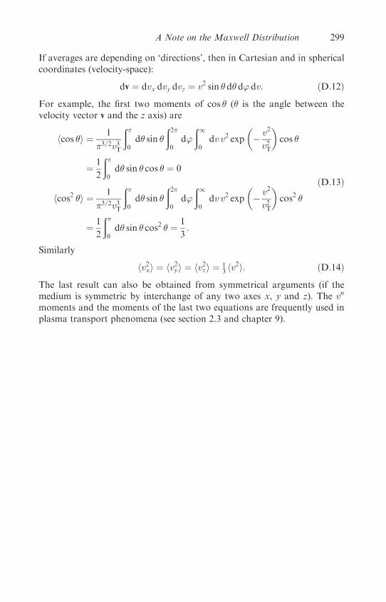
If averages are depending on ‘directions’, then in Cartesian and in sphericalcoordinates (velocity-space):

dv ¼ dvx dvy dvz ¼ v2 sin � d� d’ dv: ðD:12Þ

For example, the first two moments of cos � (� is the angle between thevelocity vector v and the z axis) are

hcos �i ¼ 1

�3=2v3T

ð�0d� sin �

ð2�0

d’

ð10

dv v2 exp

�� v2

v2T

�cos �

¼ 1

2

ð�0d� sin � cos � ¼ 0

hcos2 �i ¼ 1

�3=2v3T

ð�0d� sin �

ð2�0

d’

ð10

dv v2 exp

�� v2

v2T

�cos2 �

¼ 1

2

ð�0d� sin � cos2 � ¼ 1

3:

ðD:13Þ

Similarly

hv2xi ¼ hv2yi ¼ hv2zi ¼ 13 hv

2i: ðD:14Þ

The last result can also be obtained from symmetrical arguments (if themedium is symmetric by interchange of any two axes x, y and z). The vn

moments and the moments of the last two equations are frequently used inplasma transport phenomena (see section 2.3 and chapter 9).

A Note on the Maxwell Distribution 299

Bibliography

Abramowitz M and Stegun I A eds 1964Handbook of Mathematical Functions with Formu-

las, Graphs and Mathematical Tables, National Bureau of Standards Applied

Mathematics Series, vol 55 (Washington, DC: US Government Printing Office)

Adam J C 1982 Laser–Plasma Interaction ed R Balian and J C Adam (Amsterdam: North-

Holland)

Ahlstrom H G 1982 Physics of Laser Fusion (Springfield, VA: Livermore, US Technical

Information Service)

Alfven H 1988 Laser Part. Beams 6 437

Allen P B 1987 Phys. Rev. Lett. 59 1460

Altshuler L V 1965 Sov. Phys. Usp. 8 52

Anisimov S I and Medvedev Yu V 1979 Sov. Phys.-JETP 49 62

Anisimov S I, Kapeliovich B L and Perel’man T L 1974 Sov. Phys.-JETP 39 375

Arad B, Eliezer S, Jackel S, Krumbein A, Lobenstein M, Salzmann D, Zmora H and

Zweigenbaum S 1980 Phys. Rev. Lett. 44 326

Asay R A and Shahinpoor M eds 1993 High-Pressure Shock Compression of Solids (New

York: Springer)

Ashcroft N W and Mermin N D 1976 Solid State Physics (Fort Worth: Harcourt Brace

College Publishers)

Ashcroft N W and Sturm K 1971 Phys. Rev. B 3 1898

Babuel-Peyrissac J P, Fauquignon C and Floux F 1969 Phys. Lett. A 30 290

Backus S, Durfee III C G, Murname M M and Kapteyn H C 1998 Rev. Sci. Instrum. 69

1207

Baldis H A, Campbell EM and KruerW L 1991Handbook of Plasma Physics vol 3 Physics

of Laser Plasma ed M N Rosenbluth, R Z Sagdeev, A Rubenchik and S Witkowski

(Amsterdam: North-Holland) pp 361–434

Batani D, Bossi S, Benuzzi A, Koenig M, Faral B, Boudenne J M, Grandjouan N, Atzeni

S and Temporal M 1996 Laser Particle Beams 14 211

Bauche J, Bauche-Arnoult C and Klapish M 1988 Physica Scripta 37 659

Bell A R 1986 Laser Plasma Interaction 5 Proceedings of the 45th Scottish Universities

Summer School in Physics, 1994, ed M B Hooper (Bristol: Institute of Physics

Publishing) pp 139–68

Bernstein I B, Green J M and Kruskal M D 1957 Phys. Rev. 108 546

Bezzerides B, Forslund D W and Lindman E L 1978 Phys. Fluids 21 2179

300

Bhatnagar P L, Gross E P and Krook M 1954 Phys. Rev. 94 511

Birdsall C K and Langdon A B 1985 Plasma Physics via Computer Simulation (New York:

McGraw-Hill)

Bloembergen N 1999 Rev. Mod. Phys. 71 S283

Bobin J L 1985 Phys. Rep. 122 173

Bodner S E 1974 Phys. Rev. Lett. 33 367

——1991Handbook of Plasma Physics vol 3 Physics of Laser Plasma ed M N Rosenbluth,

R Z Sagdeev, A Rubenchik and S Witkowski (Amsterdam: North-Holland)

pp 247�70Bohm D 1949 Characteristics of Electrical Discharges in Magnetic Fields ed A Guthrie and

R K Wakerlis (New York: McGraw-Hill) p 77

Bohm D, Burhop E H S and Massey H S W 1949 Characteristics of Electrical Discharges

in Magnetic Fields ed A Guthrie and R K Waterling (New York: McGraw-Hill)

p 13

Born M and Wolf E 1980 Principles of Optics 6th edn (Oxford: Pergamon)

Boussinesq J 1871 Compte Rendus Acad. Sci. Paris 72 755

Boustie M and Cottet F 1991 J. Appl. Phys. 69 7533

Boyd T J M and Cooke D 1988 Phys. Fluids 31 651

Braginskii S I 1965 Review of Plasma Physics vol 1 ed M A Leontovich (New York:

Consultants Bureau) pp 205–311

Briand J, Adrian V, El Tamer M, Gomes A, Quemener Y, Dinguirard J P and Kieffer J C

1983 Phys. Rev. Lett. 54 38

Brown G L and Roshko A 1974 J. Fluid Mech. 64 775

Brysk H 1975 J. Phys. A8 1260

Bushman A V, Kanel G I, Ni A L and Fortov V E 1993 Intense Dynamic Loading of

Condensed Matter (Washington, DC: Taylor and Francis)

Cairns R A 1983 Laser–Plasma Interaction 2 Proceedings of the 24th Scottish Universities

Summer School in Physics, 1982, ed R A Cairns (Edinburgh: Scottish Universities

Summer School in Physics Publications) pp 1–28

Cauble R, Phillion D W, Lee R W and Hoover T J 1994 J. Quant. Spectrosc. Radiat.

Transfer 51 433

Celliers P M, Collins G W, Da Silva L B, Gold D M and Cauble R 1998 Appl. Phys. Lett.

73 1320

Chan C, Cho M H, Hershkowitz N and Intrator T 1984 Phys. Rev. Lett. 52 1782

Chandrasekhar S 1961 Hydrodynamic and Hydromagnetic Stability (Oxford: Oxford

University Press)

Chen F F 1974 Laser Interaction and Related Plasma Phenomena vol 3A ed H J Schwarz

and H Hora (New York: Plenum) p 291

——1990 Introduction to Plasma Physics (New York: Plenum)

Clemmow P C and Dougherty J P 1969 Electrodynamics of Particles and Plasmas

(Reading, MA: Addison-Wesley)

Cottet F, Hallouin M, Romain J P, Fabbro R, Faral B and Pepin H 1985 Appl. Phys. Lett.

47 678

Courant R and Friedrichs K O 1948 Supersonic Flow and Shock Waves (New York:

Interscience)

Cowan R D 1981 The Theory of Atomic Structure and Spectra (Berkeley: University of

California Press) p 12

Crawford F S Jr Waves; Berkeley Physics Course vol 3 (New York: McGraw-Hill)

Bibliography 301

Crow J E, Auer P L and Allen J E 1975 J. Plasma Phys. 14 65

Dahlburg J P, Fyfe D E, Gardner J H, Haan SW, Bodner S E and Doolen G D 1995 Phys.

Plasmas 2 2453

David F and Pellat R 1980 Phys. Fluids 23 1682

Davies R M and Taylor G 1950 Proc. Royal Soc. London A 200 375

Dawson J M 1962 Phys. Fluids 5 445

——1968 Advances in Plasma Physics vol 1 ed A Simon and W Thompson (New York:

Interscience) pp 1–66

Dawson J M and Lin A T 1974 Parametric instabilities in plasma, UCLA preprint PPG-191

Dederichs P H, Schober H R and Sellmyer D J 1981 Landolt–Bornstein 3rd edn, vol 13a

(Berlin: Springer) p 11

Dekel E, Eliezer S, Henis Z, Moshe E, Ludmirsky A and Goldberg I B 1998 J. Appl. Phys.

84 4851

DeMaria A J, Stetser D A and Heinan H 1966 Appl. Phys. Lett. 8 174

Dendy R 1993 Plasma Physics; an Introduction Course (Cambridge: Cambridge University

Press)

Denisov N G 1957 Sov. Phys.-JETP 4 544

De Resseguier T and Cottet F 1995 J. Appl. Phys. 77 3756

Diebold D, Hershkovitz N and Eliezer S 1987 Phys. Fluids 30 3308

Diels J C and Rudolph W 1996 Ultrashort Laser Pulse Phenomena (San Diego: Academic

Press)

Ditmire T, Gumbrell E T, Smith R A, Mountford L and Hutchinson M H R 1996 Phys.

Rev. Lett. 77 498

Dragila R 1987 Phys. Fluids 30 925

Drazin P G and Reid W H 1981 Hydrodynamic Stability (Cambridge: Cambridge

University Press)

DuBois D F and Goldman M V 1965 Phys. Rev. Lett. 14 544

Ehler A W 1975 J. Appl. Phys. 46 2464

Eidmen K, Meyer-ter-Vehn J, Schlegel T and Huller S 2000 Phys. Rev. E 62 1202

Einstein A 1917 Phys. Z. 18 121

Eliaz N, Moshe E, Eliezer S and Eliezer D 2000 Metall. Mater. Trans. A 31 1085

Eliezer S 1985 A stroll through the soliton theory, Institute for Fusion Studies preprint,

IFSR 164, The University of Texas, Austin, TX

Eliezer S and Hora H 1989 Phys. Reports 172 339–410

Eliezer S and Ludmirsky A 1983 Laser Particle Beams 1 251

Eliezer S and Ricci R A eds 1991High Pressure Equations of State: Theory and Applications

(Amsterdam: North-Holland)

Eliezer S, Ghatak A and Hora H 1986 An Introduction to Equations of State: Theory and

Applications (Cambridge: Cambridge University Press)

Eliezer S, Ghatak A, Hora H and Teller E 2002 Fundamentals of Equations of State

(Singapore: World Scientific)

Eliezer S, Gilath I and Bar-Noy T 1990 J. Appl. Phys. 67 715

Eliezer S, Hora H, Kolka E, Green F and Szichman H 1995 Laser and Particle Beams 13

441

Eliezer S, Paiss Y and Strauss H 1992 Phys. Lett. A 164 416

Elton R C 1990 X-Ray Lasers (Boston: Academic Press)

Evans A M, Freeman N J, Graham P, Horsfield C J, Rothman S D, Thomas B R and

Tyrrell A J 1996 Laser and Particle Beams 14 113

302 Bibliography

Evans R G 1986 Laser–Plasma Interaction 3 Proceedings of the 29th Scottish Universities

Summer School in Physics, 1985, ed M B Hooper (Edinburgh: Scottish Universities


Evely M D and Morales G J 1978 Phys. Fluids 21 1997

Fabbro R, Faral B, Virmont J, Pepin H, Cottet F and Romain J P 1986 Laser and Particle

Beams 4 413

Falthammer C G 1987 Ann. Geophys. 5A 171

Fermi E, Pasta J and Ulam S 1955 Studies of Nonlinear Problems I, Los Alamos National

Laboratory Report, LA1940

Fisher D, Fraenkel M, Henis Z, Moshe E and Eliezer S 2001 Phys. Rev. E 65 016409-1

Forslund D W, Kindel J M, Lee K, Lindman E L and Morse R L 1975 Phys. Rev. A11

679

Fortov V E, Kostin V V and Eliezer S 1991 J. Appl. Phys. 70 4524

Fraenkel M, Zigler A, Henis Z, Eliezer S and Andreev N E 2000 Phys. Rev. E 61 1899

Friedberg J P, Mitchell R W, Morse R L and Rudinski L I 1972 Phys. Rev. Lett. 28

795

Galeev A A and Natanzon A M 1991 Handbook of Plasma Physics vol 3 Physics of Laser

Plasma ed M N Rosenbluth, R Z Sagdeev, A Rubenchik and S Witkowski

(Amsterdam: North-Holland) pp 549–74

Gamaly E G 1993 Nuclear Fusion by Inertial Confinement ed G Velarde, Y Ronen and J M

Martinez-Val (Boca Raton, FL: CRC Press) pp 321–49

Gantmakher V F and Levinson Y B 1987 Carrier Scattering in Metals and Semiconductors

(Amsterdam: North-Holland)

Gardner C L, Glimm J, McBryan O, Menikoff R, Sharp D H and Zhang Q 1988 Phys.

Fluids 31 447

Gauthier J C 1989 Laser–Plasma Interaction 4 Proceedings of the 35th Scottish Universi-

ties Summer School in Physics, 1988, ed M B Hooper (Edinburgh: Scottish Universi-

ties Summer School in Physics Publications) pp 105–38

Gibbon P and Forster E 1996 Plasma Phys. Control Fusion 38 769

Gilath I, Eliezer S, Dariel M P and Kornblith L 1988 Appl. Phys. Lett. 52 1128

Ginsburg V L 1961 Propagation of Electromagnetic Waves in Plasmas (New York: Gordon

and Breach)

Glezer E N 1997 Spectroscopy and Dynamics of Collective Excitations in Solids ed

DiBartolo (New York: Plenum) p 375

Goldston R J and Rutherford P H 1995 Introduction to Plasma Physics (Bristol: Institute of

Physics)

Grady D E 1988 J. Mech. Phys. Solids 36 353

Gray D R and Kilkenny J D 1980 Plasma Phys. 22 81

Gurevich A and Pitaevski L P 1969 Sov. Phys.-JETP 29 954

Gurevich A V, Pariiskaya L V and Pitaevski L P 1965 Sov. Phys.-JETP 22 449

Gurevich A V, Pariiskaya L V and Pitaevski L P 1968 Sov. Phys.-JETP 27 476

Haan S W 1989 Phys. Rev. A 40 80

Haines M G 1980 Laser Plasma Interaction 1 Proceedings of the 20th Scottish Universities

Summer School in Physics, 1979, ed R A Cairns and J J Sanderson (Edinburgh:

Scottish Universities Summer School in Physics Publications) pp 145–218

——1989 Laser Plasma Interaction 4 Proceedings of the 35th Scottish Universities Summer

School in Physics, 1988, ed M B Hooper (Edinburgh: Scottish Universities Summer

School in Physics Publications) pp 139–70

Bibliography 303

——2001 Phys. Rev. Lett. 87 135005-1

Hargrove L E, Fork R L and Pollack M A 1964 Appl. Phys. Lett. 5 4

Hatakeyama R, Suzuki Y and Sato N 1983 Phys. Rev. Lett. 50 1203

Hazeltine R D and Meiss J D 1992 Plasma Confinement Frontiers in Physics (Redwood

City, CA: Addison-Wesley)

Hazeltine R D and Waelbroeck F 1998 The Framework of Plasma Physics (New York:

Perseus Books)

Hellwarth RW 1961Advances in Quantum Electronics ed J R Singer (New York: Columbia

University Press) p 334

Helmholtz H 1881 Ann. d. Phys. Chem. 13 385

Hershkowitz N 1985 Space Sci. Rev. 41 351

Hinton F L and Hazeltine R D 1976 Rev. Mod. Phys. 48 239

Hockney R W and Eastwood J W 1981 Computer Simulation Using Particles (New York:

McGraw-Hill)

Hoffman N M 1995 Laser Plasma Interaction 5 Proceedings of the 45th Scottish

Universities Summer School in Physics, 1994, ed M B Hooper (Bristol: Institute of

Physics Publishing) pp 105–37

Holzrichter J F 1980Laser Plasma Interaction 1 Proceedings of the 20th ScottishUniversities

Summer School in Physics, 1979, ed RACairns and J J Sanderson (Edinburgh: Scottish

Universities Summer School in Physics Publications) pp 497–606

Hora H 1969 Phys. Fluids 12 182

——1981 Physics of Laser Driven Plasmas (New York: Wiley)

——2000 Laser Plasma Physics, Forces and the Nonlinearity Principle (Bellingham, WA:

SPIE Press)

Hora H, Lalousis P and Eliezer S 1984 Phys. Rev. Lett. 53 1650

Horovitz Y, Eliezer S, Henis Z, Paiss Y, Moshe E, Ludmirsky A, Werdiger M, Arad B and

Zigler A 1998 Phys. Lett. A 246 329

Horovitz Y, Eliezer S, Ludmirsky A, Henis Z, Moshe E, Shpitalnik R and Arad B 1997

Phys. Rev. Lett. 78 1707

Horton W 1989 Phys. Rep. 192 1

Huba JD1998NRLPlasmaFormulary (Washington,DC:NavalResearchLaboratoryPub.)

Hughes T P 1980 Laser Plasma Interaction 1 Proceedings of the 20th Scottish Universities



Ichimaru S 1994 Statistical Plasma Physics vol 1 Basic Principles vol 2 Condensed Plasmas

(New York: Perseus Books)

Jackel S, Eliezer S and Zigler A 1981 Phys. Rev. A 24 1601

Jackel S, Laluz R, Paiss Y, Szichman H, Arad B, Eliezer S, Gazit Y, Loebenstein HM and

Zigler A 1982 J. Phys. E 15, 255

Kaganov M I, Lifshitz I M and Tanatarov L V 1957 Sov. Phys.-JETP 4 173

Kato Y, Mima K, Miyanaga N, Arinaga S, Kitagawa Y, Nakatsuka M and Yamanaka C

1984 Phys. Rev. Lett. 53 1057

Kauffman R 1991 Handbook of Plasma Physics vol 3 Physics of Laser Plasma ed M N

Rosenbluth, R Z Sagdeev, A Rubenchik and S Witkowski (Amsterdam: North-

Holland) pp 111–62

Kaw P, Kruer W L, Liu C S and Nishikawa K 1976 Advances in Plasma Physics vol 6 ed

A Simon and W B Thomson (New York: Wiley)

Kaw P, Schmidt G and Wilcox T 1973 Phys. Fluids 16 1522

304 Bibliography

Kelvin, Lord 1910 Mathematical and Physical Papers iv Hydrodynamics and General

Dynamics (Cambridge: Cambridge University Press)

Kentwell G W and Jones D A 1987 Physics Reports 145 319

Key M H 1980 Laser–Plasma Interaction 1 Proceedings of the 20th Scottish Universities




School in Physics, 1982, ed R A Cairns (Edinburgh: Scottish Universities Summer


——1991HandbookofPlasmaPhysics vol 3Physics ofLaserPlasma edMNRosenbluth,R Z

Sagdeev, A Rubenchik and S Witkowski (Amsterdam: North-Holland) pp 575–611

Key M H, Baumhacker H, Bigio I J, Bodner S, Brederlow G, Czuchlewski E, Fill E,

Kirillov G A, Lehmberg R H, Obenschain S P, Offenberger A A, Owadano Y,

Schroder C H, Shaw M J, Ueda K I, Volk R, Witkowski S and Witte K J 1995

Energy from Inertial Fusion ed W J Hogan (Vienna: IAEA Publication) pp 95–135

Koenig M, Faral B, Boudenne J M, Batani D, Benuzzi A and Bossi S 1994 Phys. Rev. E 50

R3314

Korteweg D J and de Vries G 1895 Phil. Mag. 39 422

Krall N and Trivelpiece A 1973 Principle of Plasma Physics (New York: McGraw-Hill)

Krokhin O N 1971 Physics of High Energy Density ed P Caldirola and H Knoepfel (New

York: Academic Press) pp 278–305

Kruer W L 1975 Nucl. Technol. 27 216

——1988 The Physics of Laser Plasma Interactions (Redwood City, CA: Addison-Wesley)

Kull H J 1991 Phys. Reports 206 197

Lalousis P 1983 PhD thesis, University of New South Wales, Australia

Lalousis P and Hora H 1983 Laser Particle Beams 1 283

Landau L D 1946 J. Phys. USSR 10 25

Landau L D and Lifshitz E M 1965QuantumMechanics, Non-Relativistic Theory (Oxford:

Pergamon Press)

——1975 Electrodynamics of Continuous Media (Oxford: Pergamon Press)

——1987 Fluid Mechanics (Oxford: Pergamon Press)

Langdon B 1980 Phys. Rev. Lett. 44 575

Langmuir I 1929 Phys. Rev. 33 954

Larson A R 1974 Calculation of laser induced spall in aluminum targets, Los Alamos

Laboratory Report LA-5619-MS

Layzer D 1955 Astrophys. J. 122 1

Lehmberg R and Obenschain S 1983 Opt. Comm. 46 1983

Lehner T 1994 Physica Scripta 49 704

——2000 Europhys. Lett. 50 480

Lifshitz E M and Pitaevskii L P 1981 Physical Kinetics (Oxford: Pergamon Press)

Liu C S and Tripathi V K 1995 Interaction of Electromagnetic Waves with Electron Beams

and Plasmas (Singapore, World Scientific)

Ludmirsky A, Givon M, Eliezer S, Gazit Y, Jackel S, Krumbein A and Szichman H 1984

Laser Particle Beams 2 2

Maiman T H 1960 Nature 187 493

Max C 1976 Phys. Fluids 19 84

McQueen RG 1991High Pressure Equations of State: Theory and Applications ed S Eliezer

and R A Ricci (Amsterdam: North-Holland)

Bibliography 305

Melrose D B 1986 Instabilities in Space and Laboratory Plasmas (Cambridge: Cambridge

University Press)

Mendel C W and Olsen J N 1975 Phys. Rev. Lett. 34 859

Meshkov E E 1969 Fluid Dynamics 4 101

Mihalas D and Mihalas B W 1984 Foundations of Radiation Hydrodynamics (Oxford:

Oxford University Press)

Milchberg H M and Freeman R R 1989 J. Opt. Soc. Am. B 6 1351

Minguez E 1993 Nuclear Fusion by Inertial Confinement ed G Velarde, Y Ronen and J M

Martinez-Val (Boca Raton, FL: CRC Press) pp 197–209

Miyamoto K 1980 Plasma Physics for Nuclear Fusion (Cambridge, MA: MIT Press)

Mocker H W and Collins R J 1965 Appl. Phys. Lett. 7 270

Morales G J and Lee Y C 1977 Phys. Fluids, 20 1135

More R M 1986 Laser Plasma Interaction 3 Proceedings of the 29th Scottish Universities



——1991 Handbook of Plasma Physics vol 3 Physics of Laser Plasma ed M N Rosenbluth,

R Z Sagdeev, A Rubenchik and S Witkowski (Amsterdam: North-Holland) pp 63–110

More R M, Zinamon Z, Warren K H, Falcone R and Murnane M 1988 J. de Physique 49

C7–43

Moshe E, Dekel E, Henis Z and Eliezer S 1996 Appl. Phys. Lett. 69 1379

Moshe E, Eliezer S, Henis Z, Werdiger M, Dekel E, Horovitz Y, Maman S, Goldberg I B

and Eliezer D 2000 Appl. Phys. Lett. 76 1555

Mulser P and van Kessel C 1977 Phys. Rev. Lett. 38 902

Nakai S, Andre M, Krupke W F, Mak A A, Soures J M and Yamanaka M 1995 Energy

from Inertial Fusion ed W J Hogan (Vienna: IAEA Publication) pp 79–95

Ng A, Celliers P and Parfeniuk D 1987 Phys. Rev. Lett. 58 214

Nicholson D 1983 Introduction to Plasma Theory (New York: Wiley)

Nishikawa K 1968 J. Phys. Soc. Jap. 24 1152

Norreys P A, Santala M, Clark E, Zepf M,Watts I, Beg F N, Krushelnick K, Tatarakis M,

Dangor A E, Fang X, Graham P, McCanny T, Singhal R P, Ledingham K W D,

Cresswell A, Sanderson D C W, Magill J, Machasek A, Wark J S, Allott R,

Kennedy B and Neely D 1999 Phys. Plasmas 6 2150

Oron D, Alon U and Shvarts D 1998 Phys. Plasmas 5 1467

Osborn R K 1972 Phys. Rev. A 5 1660

Parks G K 1991 Physics of Space Plasma, an Introduction (Redwood City, CA: Addison-

Wesley)

Pavlov V I 1979 Sov. Phys. Usp. 21 171

Peierls R E 2001 Quantum Theory of Solids (Oxford: Clarendon Press)

Perry M D and Mourou G 1994 Science 264 917

Perry M D, Pennington D, Stuart, B C, Tietbohl G, Britten J A, Brown C, Herman S,

Golick B, Kartz M, Miller J, Powell H T, Vergino M and Yanovsky V 1999 Opt.

Lett. 24 160

Pert G J 1978 Plasma Phys. 20 175


School in Physics, 1985, ed M B Hooper (Edinburgh: Scottish Universities Summer


Pomraning G C 1973 The Equations of Radiation Hydrodynamics (New York: Pergamon

Press)

306 Bibliography

Raadu M A 1989 Phys. Rep. 178 25

Rand S 1964 Phys. Rev. 136 B231

Raven A, Willi O and Rumsby T P 1978 Phys. Rev. Lett. 41 554

Rayleigh, Lord 1876 Phil. Mag. 1 257. Also Scientific Papers vol 1 (Cambridge: Cambridge

University Press) pp 251–71

——1883 Proc. London Math. Soc. 14 170

Richtmyer R D 1960 Commun. Pure Appl. Math. 13 297

Robieux J 2000 High Power Laser Interactions (London: Intercept Pub.)

Rosen M D 1984 Comm. Plasma Phys. Cont. Fusion 8 165

Rosenberg Z, Luttwak G, Yeshurun Y and Partom Y 1983 J. Appl. Phys. 54 2147

Rosenbluth M N 1972 Phys. Rev. Lett. 29 565

Rosenbluth M N, MacDonald W M and Judd D L 1957 Phys Rev. 107 1

Russell J S 1844 Reports on Waves 14th Meeting of the British Association for the

Advancement of Science (London: John Murray) pp 311–90

Saeki K, Iizuka S and Sato N 1980 Phys. Rev. Lett. 45 1853

Salzmann D 1998 Atomic Physics in Hot Plasmas (Oxford: Oxford University Press)

Sargent III M, Scully M O and Lamb Jr W E 1974 Laser Physics (Reading, MA: Addison-

Wesley)

Schlessinger L and Wright J 1979 Phys. Rev. A20 1934

Schmidt G 1966 Physics of High Temperature Plasmas, An Introduction (New York:

Academic)

Sheng Z M and Meyer-ter-Vehn J 1996 Phys. Rev. 54 1833

Shkarofsky I P, Jonston TW and Bachynski M P 1966 The Particle Kinematics of Plasmas

(Reading, MA: Addison-Wesley)

Shvarts D 1986 Laser Plasma Interaction 3 Proceedings of the 29th Scottish Universities



Shvarts D, Alon U, Ofer D, McCrory R L and Verdon C P 1995 Phys. Plasmas 2 2465

Siegman A E 1986 Lasers (Mill Valley, CA: University Science Books)

Sigel R 1980 Laser Plasma Interaction 1 Proceedings of the 20th Scottish Universities



Silin V P 1965 Sov. Phys.-JETP 20 1510

——1965a Sov. Phys.-JETP 21 1127

Skupsky S, Short R W, Kessler T, Craxton R S, Letzring S and Soures J M 1989 J. Appl.

Phys. 66 3456

Smith R A 1987 Laser Particle Beams 5 381

Spence D E, Kean P N and Sibbett W 1991 Opt. Lett. 16 42

Speziale T and Catto P 1977 Phys. Fluids 20 1420

Spitzer L 1962 Physics of Fully Ionized Gases 2nd edn (New York: Interscience)

Spitzer L and Harm R 1953 Phys. Rev. 89 977

Stamper J A 1991 Laser Part. Beams 9 841

Stamper J A and Tidman D A 1973 Phys. Fluids 16 2024

Stamper J A, Papadopoulos K, Sudan RN, Dean S O,McLean EA and Dawson JM 1971

Phys. Rev. Lett. 26 1012

Steiger A D and Woods C H 1972 Phys. Rev. A 5 1467

Steinberg D J 1996 Equation of State and Strength Properties of Selected MaterialsUCRL-

MA-106439, Livermore, CA, USA

Bibliography 307

Stix T H 1992 Waves in Plasmas (New York: American Institute of Physics)

Strickland D and Mourou G 1985 Opt. Commun. 56 219

Svelto O 1976 Principle of Lasers (New York: Plenum)

Tajima T 1989 Computational Plasma Physics with Applications to Fusion and Astrophysics

Frontiers in Physics (Redwood City, CA: Addison-Wesley)

Takabe H, Mima K, Montierth L and Morse R L 1985 Phys. Fluids 28 3676

Taylor G 1950 Proc. Roy. Soc. A 201 192

Thompson W B 1962 An Introduction to Plasma Physics (Reading, MA: Addison-Wesley)

Thyagaranjan K and Ghatak A K 1981 Lasers, Theory and Applications (New York:

Plenum)

Trainor R J, Shaner, J W, Auerbach J M and Holmes N C 1979 Phys. Rev. Lett. 42 1154

Trubnikov B A 1965 Review of Plasma Physics vol 1 ed M A Leontovich (New York:

Consultants Bureau) pp 105–204

van Kessel C G M and Sigel R 1974 Phys. Rev. Lett. 33 1020

Veeser L R, Solem J C and Liebar A J 1979 Appl. Phys. Lett. 35 761

Wang X W and Downer M C 1992 Opt. Lett. 17 1450

Washimi H and Taniuti T 1966 Phys. Rev. Lett. 17 996

Wharton K B, Hatchett S P, Wilks S C, Key M H, Moody J D, Yanovsky V, Offenberger

A A, Hammel B A, Perry M D and Joshi C 1998 Phys. Rev. Lett. 81 822

Wickens L M, Allen J E and Rumsby P T 1978 Phys. Rev. Lett. 41 243

Woan G 2000 The Cambridge Handbook of Physics Formulas (Cambridge: Cambridge

University Press)

Woo W, Estabrook K and DeGroot J S 1978 Phys. Rev. Lett. 40 1094

Yamanaka C 1991 Introduction to Laser Fusion (London: Harwood Academic)

Zabusky N J and Kruskal M D 1965 Phys. Rev. Lett. 15 240

Zeldovich Ya B and Raizer Yu P 1966 Physics of Shock Waves and High-Temperature

Hydrodynamic Phenomena ed Hayes W D and R F Probstein (New York: Academic

Press)

Zhou J P, Taft G, Huang C P, Murnane M M and Kaptyn H C 1994 Opt. Lett. 19, 1149

Zinovev V E 1996Handbook of Thermophysical Properties of Metals at High Temperatures

(New York: Nova Science)

308 Bibliography

Index

ablation

plasma 257

steady-state 180

ablation (surface) instability 264, 265, 268

ablation pressure 177, 183, 219, 255

ablation rate 258

ablation rate, mass 266

ablation stabilization 257

ablation surface 43, 44, 45, 177, 179, 181, 197,

198, 233, 266, 268

absorbed laser energy 140

absorption 28, 31, 32, 43, 78, 87, 94, 95, 106,

108, 157, 169, 173, 174, 175, 180, 205

absorption coefficient 18, 29, 54, 74,76, 78, 79,

88, 90, 91, 96, 97, 98, 103, 160, 173

absorption coefficient, inverse bremsstrahlung

161, 162

absorption domain 43

acceleration continuity 276

acceleration of a thin foil 241

acoustic wave 73, 105, 106, 121, 215, 216

adiabatic exponent 38

adiabatic oscillations 70

adiabatic process 218

Airy function 84, 85, 86, 95

Alfven dispersion relation 169

Alfven wave 145, 168

Alfven wave velocity 169

Ampere–Maxwell law 285

amplifier 7, 8, 9, 10, 12, 13

amplitude

elastic 111

off-resonance 116

power absorption 111

amplitude of oscillations 112

amplitude of the wave 125

angle of deflection 185

angle of rotation 155, 156

angular diffusion 195

angular momentum 159, 258

angular momentum conservation 160, 161

anisotropic 195

anisotropic electron distribution 196

anvils 213

aspect ratio 183, 255

astrophysics 73, 143

asymptotic expansion 86

asymptotic steady state 270

atomic physics 3

Atwood number 254, 257, 263

averaging over the initial positions 114

Avogadro’s number 56

axisymmetric beam 160

B integral 13

backscattered wave amplitude 123

backscatter electromagnetic wave 121

back surface velocity 245

ballistic research 249

band, conduction 103

bandwidth 11, 12

Bernoulli equation 272

BGK model 57

binding energy 241

black body radiation 2

Bloch-electron band 98

blow-off velocity 44

body forces 53

Boltzmann distribution 3, 16

Boltzmann equation 57, 58, 59, 60, 189, 194,

196, 197

Boltzmann–Vlasov equation 55

309

Bose–Einstein distribution 100

boundary conditions on the interface 276

boundary equation 276, 279

boundary value equation 278

bremsstrahlung 27, 28, 74, 198, 199, 211

bremsstrahlung, inverse 27, 28, 74, 76, 77, 78,

91, 98, 109

bremsstrahlung, nonlinear 78

brightness 6, 7, 27

Brillouin instability 40, 122

Brillouin zone 98, 100

brittle materials 250

broadening, collisional 5

broadening, Doppler 5

broadening, homogenous 5

broadening, inhomogeneous 5

broadening, line 4, 5

Brownian motion 190

bubble formation 255

bubble surface equation 272

bulk modulus 241, 245, 246, 247

bulk sound speed 227

buoyancy force 257, 272

Caviton 65, 141

cavity 1, 6, 9, 11, 133

centre of mass (CM) 20, 147, 183, 184, 185,

186, 192, 193

centre of mass energy 18

centre of mass velocity 60

characteristic curves 218

characteristics 230

charge collectors 141

charge fluctuation 35

charge neutrality 69, 80, 121, 136, 147, 148,

177, 196, 203

charge separation 118, 141

chemical explosives 213

chemical potential 101

chirped pulse amplification (CPA) 1, 12, 13

circularly polarized laser 154, 157, 159, 160

circular polarization, left-handed 165

circular polarization, right-handed 165, 166

closest approach 19, 21, 34, 75, 186

cloud in cell 63

coherence, spatial 6, 7

coherence, temporal 6

coherent oscillations of the electrons 123

cohesion energy 241, 242, 245

cold electron 177, 178, 203, 242, 243

cold (electrons) pressure 44, 242, 243, 245,

247

cold temperature 180

collision

binary 34, 57

direct 57, 62

electron 94

electron–electron 74, 99, 101, 104, 160, 179,

187, 195

electron–ion 20, 22, 51, 54, 58, 74, 87, 94,

123, 187

electron–phonon 99, 101, 104

instantaneous 22

collision frequency 17, 19, 20, 23, 24, 41, 57,

76, 102, 118, 160,188, 195

collision frequency, effective 58, 94

collision frequency, electron 97, 99

collision frequency, electron–ion 21, 41, 78,

90, 91, 123, 173, 195

collision frequency, velocity-dependent 105

collision term 189, 190

collision times for large-scale scattering 187

collisional absorption 74

collisionless damping 40

collisionless energy exchange 114

collisions, large angle 62

collisions per unit time 200

compressibility 241

compression domain 43

compression wave 231, 232

compressor 13

conduction band 54, 55

conservation

centre of mass energy 192

charge 36, 147, 285

electromagnetic field energy 286

energy 47, 49, 50, 51, 53, 54, 60, 87, 99, 100,

102, 103, 115, 122, 143, 149, 184, 187,

205, 207, 208, 210, 214, 223, 234, 235,

236, 237

mass 37, 47, 48, 58, 59, 146, 147, 207, 214,

217, 218, 222, 223, 233, 234, 237, 260,

267, 275, 278, 280

momentum 37, 47, 48, 50, 51, 52, 53, 59, 60,

70, 71, 72, 89, 100, 115, 121, 122, 127,

135, 136, 145, 146, 162, 168, 169, 184,

192, 203, 214, 217, 218, 222, 233, 235,

237, 260, 266, 272, 275, 276, 280

radiation energy 33

conservation equations 56, 280

conservation laws 47, 106, 107, 108, 226, 286

constitutive equations 285

continuity equation 42, 48, 53, 55, 58, 59, 70,

71, 119, 136, 147, 158, 203, 269, 286

310 Index

continuity equation, for ions 135

continuity equation in the velocity space

191

continuity of the normal magnetic induction

field 234, 237

continuity of the parallel electric field 234, 237

convection of the magnetic field 152

convection of the plasma fluid 149, 151

converging shocks 259

coordinates

Cartesian 26, 56, 58, 81, 154, 163, 168, 193,

235, 260, 261, 270, 292, 299

cylindrical 160, 161, 292

Eulerian 51, 52, 53

Lagrangian 51, 52, 53

spherical 18, 20

coordinates moving with the flow 218

corona 43, 44, 55, 76, 136, 137, 143, 175, 178,

179, 180, 182, 188, 189, 198, 233, 257

correlation function 74

corrugated interface 258, 274, 277

corrugation of the shock surfaces 279

cosmic radiation 23

Coulomb collision 184

Coulomb cutoff coefficient 186

Coulomb gauge 288, 289

Coulomb logarithm 177, 189

Coulomb potential 289

Coulomb scattering 189

coupling energy 52

crack propagation 250

critical density 30, 44, 76, 77, 94, 80, 84, 106,

135, 173, 156, 157, 159

critical surface 43, 45, 83, 84, 85, 87, 92, 93,

94, 106, 133, 175, 176,177, 179, 181, 197,

206, 233

cross section 17, 18, 19, 21, 23, 24, 31, 34, 185,

186, 200

cross section, differential 19

cross section, inverse bremsstrahlung 32

cross section, photoelectric 32

cross section, Rutherford 19

cross section, total 18, 19, 20

cutoff 164, 165, 166

cutoff wavenumber 266

cyclotron frequency 164, 167

damping 87, 88, 93, 94, 109, 110, 115, 120,

123, 173

collisional 109, 112, 124

collisionless (see Landau damping) 109

spatial 78

damping rate 116

damping rate, spatial 76

de Broglie scale length 199

de Broglie wavelength 21

Debye length 20, 33, 34, 35, 36, 64, 69, 75,

127, 129, 138, 145, 186

Debye length, electron 62

Debye shielding 35, 189

Debye solid-state theory 243

Debye sphere 35, 45, 58, 62

decay instability 107, 108, 109

deflagration 257

degrees of freedom 38, 55, 111, 206

delta function, Dirac 4, 34, 61, 114, 141, 206,

264, 265, 273

density

background 121, 136

high frequency 119

low frequency 119

momentum 121

pump energy 117

steep 91

density fluctuation, electron 115

density fluctuation, ion 115

density jump 264

density profile, linear 77, 84, 87, 89, 90, 95

density ripple 118

derivative of the bulk modulus 245

derivatives along the characteristics 219

detailed balance 32

dielectric 40, 41, 42, 66, 67, 154, 156

dielectric coefficient 173, 236, 285

dielectric function 40, 41, 42, 80, 87, 90, 93,

94, 97

dielectric function, complex 94

dielectric permittivity 96, 98

dielectric tensor 170

diffraction limited 7

diffusion 24, 26, 60, 189, 191

anomalous 25

Bohm 26

classical 25

parallel 183

transverse 183

diffusion approximation 178, 197

diffusion coefficient 24, 25, 58

diffusion equation 24, 206

diffusion flux 197

diffusion in angular space 195

diffusion in velocity space 195

diffusion relaxation time 152

diffusivity 215

Index 311

dimension

1D 63

1.5D 63

2D 63

2.5D 63

3D 63

dimensional analysis 215

dispersion relation 39, 40, 42, 68, 69, 71, 72,

73, 75, 76, 89, 90, 99, 105, 106, 107, 108,

129, 155, 156, 162, 163, 164, 165, 166,

167, 169

dissipation 5, 94, 125, 129

dissipative forces 232

dissipative phenomenon 226

dissipative radiative processes 17

distribution, energy 31

distribution, isotropic 21

diverging shocks 259

Doppler effect 4

double layer (DL) 135, 138, 141, 143, 176, 180

downstream variables 222, 237

drag force 257, 272

drift velocity 58

driving force 105, 115

Drude model 22, 149

ductile materials 249

Dulong–Petit law 55

Dulong–Petit value 244

dynamo effect 144, 153

echelons 238

effective mass, electron 101

e-folding time 254

eigenfunction 262

eigenstate, energy 15

eigenstate, ion 27

eigenvalue 115

imaginary 118

eigenvalue equation 262

eigenvalue frequency 112

Einstein coefficients 2, 3

electrical conductivity 22, 23, 24, 41, 96, 97,

98, 99, 102, 149, 151, 266

electrical conductivity coefficient 80, 148, 177

electrical discharges 5

electric charge separation 69, 70

electric current 22, 41, 61, 79, 155, 158, 159,

162, 177, 196, 266

electric displacement 284

electric field

high-frequency 134

low-frequency 134

electric field phase 113

electric field strength 284

electric induction 284

electric polarization 285

electric potential 137, 138

electric potential energy 189

electromagnetic backscattered wave 122

electromagnetic energy density 285, 286

electromagnetic field momentum 66

electromagnetic field, high frequency 65

electromagnetic field, scattered 121

electromagnetic force 49, 285

electromagnetic modes 8, 9

electromagnetic sources 41, 42, 288

electromagnetic wave decaying 115

electromagnetic wave equation 122

electron, bound 16, 27, 28

electron conduction 179, 180

electron conductivity 205

electron cyclotron frequency 154, 170

electron cyclotron wave 166, 167

electron distribution function 195, 197

electron drift motion 189

electron effective mass 102

electron energy transport 189

electron fluid 33, 50, 51

electron fluid velocity 127, 136

electron inertia 72, 168

electron–ion scattering 188

electron oscillation frequency 30, 72, 73

electron–phonon interaction 55

electron–photon interaction 211

electron plasma frequency 106, 115, 123, 163

electron plasma frequency in the dielectric

155

electron (plasma) wave 71, 91, 94, 105, 106,

107, 109, 112, 115, 116, 117, 201

electron plasma wave (see also plasmon) 36,

39, 69

electron pressure 127, 150

electrons, degenerate 45

electron temperature 50, 52, 95, 102, 106, 118,

121, 127, 136, 137, 199, 201, 218

electron thermal conduction 176, 211

electron thermal motion 243

electron trajectory 200

electron transport 179

electron velocity distribution 20

electron velocity distribution function 178,

201

electrostatic plasma wave, high frequency 105

electrostatic potential 33, 34, 140, 203

312 Index

electrostatic wave 172, 173

elliptical rotation of the electric field 164

emissivity 31

energy

kinetic 189, 223, 241, 297

potential 297

thermal 241

energy band 28

energy conservation rate 123

energy deposition depth 54

energy equation, electron 54

energy equation, ion 54

energy exchange, electron–ion 100

energy exchange, electron–phonon 100

energy flow 60

energy flux 123, 287

energy loss 183, 188, 200

energy radiated per unit time by an electron

201

energy rate exchange 114

energy relaxation time 188

energy relaxation, electron 104

energy relaxation, ion 104

energy transfer rate 99

energy transport 179, 205

energy, internal 223

enthalpy 181

entropy 38, 203, 218, 220, 224, 226, 237, 247

entropy jump 226

equation, for magnetic field 151

equation of motion 33, 60, 61, 68, 74, 154

equation of state 24, 26, 33, 35, 37, 45, 47, 50,

51, 52, 53, 55, 57, 70, 149, 180, 207, 224,

225, 226, 228, 230, 231, 237, 241, 244,

245, 247, 248, 252, 275

equation of state, (semi-empirical) wide range

252, 253

equilibrium distribution 178, 189

Eulerian mass 52

Eulerian position 52

Eulerian space derivative 52

Eulerian time derivative 52

excited state 15

expanding plasma into the vacuum 135

exploding foils 213

exponential profile 77

external energy deposition 50

external force 110, 235, 260

external potential 35

extraordinary (electromagnetic) wave 145,

162, 163, 164, 165, 172

extraordinary mode 171

Faraday effect 10, 144, 153, 157, 168

Faraday–Maxwell equation 161

Faraday’s law 285

fast electron preheat 239

fast electrons 141, 177, 241

fast ions 140, 141

Fermi–Dirac distribution 45, 101

Fermi energy 55, 101

Fermi momentum 101

Fermi–Pasta–Ulam problem 126

Fermi surface 98

Fermi temperature 101, 104

Fermi velocity 101, 103

field envelope 12

filamentation 13, 65

filaments 180

finite-difference approach 62

first moment 191

first-order equations 70

first-order variations 70

flow patterns 256

fluctuation 127, 153, 250

fluid, electron 69, 146

fluid element 220

fluid equations 47, 50, 53, 55, 122, 203, 223

fluid equations of two temperatures 51

fluid equations, electron 118

fluid equations, ion 35, 118

fluid, ion 69, 146

fluid models 138

fluid particle 26, 48, 52

fluid-Poisson equations 127, 128, 129

fluids energy equations, two 51

fluid theory 55, 56

fluid variables 52

flux

absorbed laser 182

energy 180

heat 23, 177, 197, 205, 209

heat energy 52

laser energy 144

mass 180

momentum 26, 180

flux conservation

energy 181

mass 181

momentum 181

particle 17, 23, 25

flux continuity 139

flux of the electromagnetic energy 285

foil reference frame of coordinates 264

Fokker–Planck collision 58, 196

Index 313

Fokker–Planck equation 189, 190, 191, 192,

194, 195, 196, 197

force

frictional drag 110

inertial 151

periodic external 112

viscous 151

force per unit volume 66

forced harmonic oscillator 109

Fourier components 63

Fourier modes 128

Fourier transform 11, 110, 116, 119, 129, 163,

166, 168, 169, 261

Fourier transport 200

fracture, dynamic 249

frame of reference of the moving interface 274

free current density 284

free electric charge density 284

free electron model 244

free energy 14, 15

free-streaming flow of electrons 198

free streaming flux 178, 197

free streaming plasma 181

free streaming velocity 113

free surface 228, 251

free-surface velocity 230, 231, 240, 245, 251

frequency components, fast 119

frequency components, low 119

frequency electric fields, high 134

frequency electric fields, low 134

frequency modulation 11, 12

frequency, complex 40

full frequency width at half maximum 111

full width half maximum (FWHM) 4

fully ionized plasma 195, 218

fusion 59

gain 8, 10

gamma function 209

gauge 288

Gauss divergence theorem 234, 294

Gauss equation 70

Gauss–Faraday law 285

Gauss’s law 285

Gauss’ theorem 47, 49

Gaussian profile 5, 9, 152

Gaussian pulse 11

Gaussian shape 5

Gaussian velocity distribution 63

geometrical optics 89

geometry, cylindrical 162

geometry, plane 52, 135, 162, 182, 183

global neturality 138, 139

grating 13

gravitation 254, 255, 260, 264

gravitational force 49

Green’s first and second theorem 294

Green’s function 152

grid points 63

grid spacing 62, 63

ground state 15

group velocity 12, 39, 71

growth rate 118, 257, 258

growth rate of the backscattered wave

amplitude 123

Gruneisen coefficient 243, 249

Gruneisen equation of state 234, 244, 247, 248

Gruneisen parameter 249

gun drivers of plates 252

gyro motion 35

gyroradius, electron 35

Hall effect 149

Hamiltonian 15, 56

harmonic driving force 110

harmonic motion 37, 110

harmonic oscillations 110

heat capacities at constant volume, electron

102

heat capacities at constant volume, ion 102,

103

heat capacities, constant pressure 180, 218

heat capacities, constant volume 24, 180, 181,

218

heat capacity 24

heat capacity, electron 54, 99

heat capacity, lattice 54

heat carriers 205

heat conduction 53, 205

heat conduction coefficient 152

heat conduction by photons 211

heat conduction equation 207

heat conductivity, electron 99, 101, 103

heat deposition 98

heat diffusion equation 151

heat flow 23, 176, 178, 197, 198, 214

heat flux, differential 197

heat transfer 195

heat transport 24, 51, 60, 178, 198, 205

heat transport, electron 212

heat transport equation 206

heat wave 7, 175, 205, 211, 214, 216

heat wave equation 214

heat wave front 216

314 Index

heat wave temperature space profile 209

heat wave velocity 209, 214, 215

Helmholtz equation 96

high energy electrons 74

high energy ions 140

highest laser-induced pressure 230

high-frequency (electron) wave equation 120

high-frequency phenomena 144

high-Z atoms 28

homogeneous equations 288

homogeneous medium 66, 75, 77, 79, 80, 126

hot electrons 44, 45, 91, 177, 180, 198, 291,

202

hot electrons pressure 44

hot electron temperature 240

hot spots 180

Hugoniot 221, 225, 230, 232, 243, 245, 277

Hugoniot curve 224, 225, 228, 229, 242, 243

Hugoniot energy relation 248

Hugoniot equation of state 227

Hugoniot pressure 242, 246, 247, 249, 251

Hugoniot relations 224, 276, 277

hydrodynamic effects 215

hydrodynamic efficiency 182

hydrodynamic equations 37, 260

hydrodynamic expansion 96

hydrodynamic instabilities 45, 162, 183, 254,

256, 258, 269

hydrodynamic theory 36, 47

hydrogen-like atom 32

hydrogen-like model 16

ideal gas equation of state 145, 149, 150, 181,

218, 226

ignition 205, 255

impact parameter 19, 20, 75, 183, 185, 189,

200

impedance matching 228, 229, 245

implosion pressure 255

implosion velocity 255

imprint (a disturbance) 256

imprint, laser initial 257

impulsive acceleration 258, 273, 274

incoherence, spatial 238

incoherent 3

incompressibility assumption 265

incompressible fluid 26, 261, 270, 272, 273

incompressible plasma 266

index of refraction 29, 30, 153, 155, 164,

166

complex 96

extraordinary 171

nonlinear 11, 13, 42

ordinary 171

indices of refraction for right and left

polarization 166

induced transition 3

induced emission 31

induced emission lifetime 3

inertia of the electron 127, 145

inertial confinement fusion (ICF) 6, 162, 175,

179, 183, 205, 254, 256, 257, 258

inertial term 203

inhibited thermal transport 215

inhibition factor 178, 197, 198

inhomogeneous equations 288

inhomogeneous plasma 68, 79

inhomogeneous system 120

inhomogeneous wave equation 288

initial value problem 127

instability seeds 256

inter-atomic forces 252

inter-band absorption 98

interface equation 276

intermixing 255, 256

internal energy 49, 181, 237, 243

intra-band absorption 98

inverse Faraday effect 145, 157, 159, 161,

162

inverse matrix 170

inviscid (no viscosity) 279

ion frequency 79

ion (plasma) wave 73, 105, 106, 107, 108, 109,

112, 115, 117, 129

ion-acoustic instability 40

ion acoustic phase velocity 129

ion acoustic wave 122, 126, 127

ion cyclotron frequency 169

ion density fluctuation 118

ion density perturbation 121

ion density wave amplitude 122

ion fluid 50, 51

ion force (momentum) 119

ion lattice 54

ion local temperature 33

ion oscillation frequency 72, 73

ion pressure 44

ion temperature 52, 102, 106, 121, 127, 136,

218

ionization 14, 15, 17, 31, 58, 74, 103, 106, 118

ionization energy 16

ionization potential 15

ion-plasma frequency 134

irreversible process 19

Index 315

irreversible thermodynamics 178

irrotational fluid 270

isentrope (process) 38, 217, 219, 224, 225, 230,

242, 247, 250, 277

isentrope pressure 247

isentropic curves 224

isentropic expansion 251

isentropic flow 218, 219

isolator 7, 8, 10

isotherm 224, 252, 253

isothermal electron equation 71

isothermal speed of sound 137, 182, 183

isotropic 30, 31, 195

isotropic pressure 59

Joule heating 97, 235, 236

jump condition 223, 233, 234, 236, 237, 277,

281, 282

jump equations 227, 233

jump in the potential 204

KdV (Korteweg and De Vries) equation, 125,

126, 127, 131, 132

Kelvin–Helmholtz instability 40, 258, 260,

283

Kerr cell 1, 9

kinematic theory 47

kinematic viscosity 151, 152

kinetic energy of the electron 201

Kirchhoff’s law 32

laboratory coordinates 183

laboratory frame (of reference) 20, 183, 184,

187, 192, 222, 223, 226, 231

Lagrangian coordinates 261

Landau damping 40, 63, 93, 109, 115, 117,

123, 124, 173

Langmuir wave 105

Laplace equation 270

Laplacian 292

large angle deflection 186

large angle scattering 186

large deflection 187, 190

large-scale deflection 189

Larmor angular frequency 179

Larmor radius 35, 189

laser

CO2 7

gas 5, 7

helium-neon 1

iodine 7

KrF 7

megajoule 8

neodymium glass 1, 7, 10, 141

solid state 7

Ti–sapphire 1, 7

x-ray 175

laser diode 5, 10

laser divergence 6, 7

laser electric field amplitude 134

laser energy deposition 54

laser energy fluency 8

laser energy flux 134, 284

laser intensity profile 98

laser irradiance non-uniformity 238

laser pump 108

laser pump amplitude 121

laser radius 135

laser scattering 106

laser spot 135

laser uniformity 256

lateral rarefaction wave 238

lattice specific heat at constant volume 243

left-handed circular polarization (LHCP) 153,

154, 155

light amplification 6

line absorption 27, 28

line broadening 28

line emission 27, 28

line shape 5

line shape function 4

line shape, natural 4

line width, natural 6

linear analysis 260

linear differential equation 127

linear equations 119

linear momentum 160

linear polarized (laser) electric field 153, 155,

168

linear theory 275

linear trajectory 69

linearization procedure 38, 70, 72, 128, 166,

261, 266

linearized equations 119, 162

linearized Maxwell equation 267

linearized momentum equation 267

Liouville’s theorem 55, 56

longitudinal phonon mode 100

longitudinal sound velocity 99

longitudinal wave 39, 76, 164

Lorentz equation 61, 68

Lorentz force 286

Lorentz gauge 288

Lorentzian profile 4, 5

316 Index

Lorentzian pulse 11

Lorentz law 285

Lorenz plasma 196

low-frequency electric field 119

L-wave 168

Mach number 226, 232

macroinstabilities 39

macroscopic electric fields 134

macroscopic quantity 58

macroscopic scale length 151

magnetic compression 213

magnetic field

axial 153, 158, 159, 161, 162

diffusion of 151

external 172

steady-state (d.c.) 144, 150, 154, 155, 162,

163, 168, 169, 170, 171

toroidal 144, 145, 146, 150, 153, 176

magnetic field amplitude, laser 144

magnetic field diffusion time 152

magnetic field generation 65

magnetic fluid 146

magnetic flux density 284

magnetic monopoles (poles) 234, 285

magnetic permeability 155, 285

magnetic polarization 285

magnetic pressure 233

magnetic Reynolds number 144, 151, 152, 153

magnetized plasma 162,173, 174, 179

magneto-hydrodynamic equations 144, 149

magneto-hydrodynamics 146

Markov process 190

matrix element 99, 100

maximum possible compression 246

maximum possible growth of the instability

120

Maxwell distribution 20, 45,55, 57, 62, 176,

177, 178, 188, 198, 199, 297, 298

Maxwell equations 36, 38, 41, 42, 47, 50, 61,

66, 67, 70, 75, 80, 91, 94, 144, 145, 146,

149, 154, 158, 162, 168, 169, 171, 234,

235, 266, 284, 285, 286, 287, 288

Maxwellian distribution, equilibrium 195

Maxwellian double electron distribution 199

mean decay time 111

mean free path 17, 18, 19, 24, 31, 34, 35, 178,

186, 198, 211

mean free path, electron 177, 196, 206, 240

mean free path for hydrogen-like plasma 211

mean squared velocity 63

melting temperature 101

metallurgical cross section 250

metric elements 292

microinstabilities 39

mirror symmetry 208

mixing zone between the fluids 258

mode locking 1, 9

molecular collision 190

moment (definition) 60

moment equation 58, 60

moment equation, zero 59

moment of velocity 298

momentum, electron 147

momentum exchange 60

momentum, ion 147, 148

momentum jump conditions 235

momentum loss 183, 187, 188

momentum loss-relaxation time 187

momentum of the gas 222

momentum relaxation rate, electron 99, 101,

102,103

momentum transfer 65

monoatomic gas 181

monochromatic wave 75, 96, 169

monopoles 269

motion

high-frequency 118

low frequency 118

quasi-neutral 118

multimode perturbation 258

multiple Coulomb collisions 177

multiple scattering 188

multiple small-angle collisions 190

multiple small-angle scattering 189

Navier–Stokes equation 26

negative pressure (tension) 251

neutral plasma 187

neutralizing background 33

Newton equation for electrons 142

Newton’s law 22, 37, 41, 48, 52, 63, 79, 112,

222

non-isotropic medium 285

nonlinear differential equation 127

nonlinear dispersion relation 129

nonlinear drag force 256

nonlinear effect 138, 231

nonlinear equations 116

nonlinear evolution of the RT instability 258

nonlinear force 65, 69

nonlinear heat wave 210

nonlinear induced magnetic field 159

nonlinear interaction 126

Index 317

nonlinear integral-differential equations 195

nonlinear localized wave 126

nonlinear mass string (Fermi, Pasta and

Ulam) 125

nonlinear phenomenon 105

nonlinear plasma effects 64

nonlinear polarizability 105

nonlinear transport coefficients 205

nonlinear wave 125

nonlinear wave phenomena 201

non-local transport 198

non-Maxwellian electron velocity distribution

140

non-uniformity of the laser beam 179

normal mode 255, 256, 261

Nova laser 213

nuclear reaction 7

number of degrees of freedom 181

Ohm heating 50

Ohm’s law 22, 25, 148, 285

Ohm’s law, generalized 25, 144, 146, 147, 149

Onsager relations 178

opacity 31

optical fibre 13

optical smoothing techniques 238

optical spectrum 3

ordinary (O-mode) wave 145, 162, 163, 165,

172

orthogonal frame of reference 191, 194

ORVIS (optically recording velocity

interferometer system) 230

oscillating two-stream instability 118

oscillations

critically damped 110

forced 110, 111

high-frequency 127, 136

over-damped 110

weakly damped 110

oscillator 7, 8, 9, 13

oscillator, forced harmonic 110

oscillator, harmonic 115

out-flowing plasma 221

parabolic initial density profile 141

parabolic laser profile 161

parametric (decay) instability 40, 65, 106, 105,

108, 109, 110, 115, 116, 118, 120

particle, charge collector 11

particle flow velocity 214, 228, 230, 241, 250,

251

particles, free-streaming 139

particle in cell (PIC) 61, 62

particle simulation code 47

particle simulations 61, 62

particle theory 47, 61

partition function 15

pellet, spherical 140

permeability 68, 287

permittivity 66, 285, 287

phase 6

phase plate 238

phase shift 88

phase space 55, 56, 57, 190, 194

phase space trajectory 56

phase transition, solid–solid 233

phase transitions 245

phase velocity 5, 39, 71, 74, 112, 124, 129, 164,

168

phonon 54, 100

phonon dispersion relation 100

phonon energy 103

phonon spectrum 99

photoelectric effect 27, 28

photoionization 27, 28

photon distribution function 29

photon energy spectrum 199

photon momentum 89

photon wave 107, 108

planar collision 230

planar symmetry 216, 219

planar waves 277

planarity 238

Planck function 30, 31

Planck’s law 2, 16

plane-polarized light 153

plane wave 7, 168

plasma

ideal 45

neutral 139

slab of 37

strongly coupled 45, 189

two component 127

plasma frequency 106, 118, 128, 145, 164

plasma expansion into vacuum 137, 203

plasma fluid 26

plasma frequency 37, 54, 62, 65

plasma heating 265

plasma instabilities 256

plasma lifetime 64

plasma neutrality 103

plasma oscillation 36, 37

plasma parameter 35

plasma–vacuum boundary 91

318 Index

plasma–vacuum interface 82, 84, 85

plasma wave amplitude 40

plasmon 39, 71, 105, 106, 124

plastic deformation 249

Pockels cell 9

Pockels effect 10

Poisson equation 34, 36, 70, 71, 118, 119, 141,

193, 285

polarization force 49

polarization of the dielectric medium 155

polarization plane 10

polarization, p- 88, 91, 92, 93, 94, 95, 172,

173, 174

polarization, s- 88, 90, 95, 172

polarized electromagnetic field, linear 81, 82

polarized light, linear 10, 96

polarizer 10

ponderomotive force 65, 66, 67, 68, 69, 70, 71,

105, 118, 119, 134, 135, 133, 159

ponderomotive force, Landau–Lifshitz 65

ponderomotive pressure 72, 73

population inversion 6, 9

potential barrier 139

potential equations 288

potential force 203

potential jump 138

power density balance 115

power radiated by the electron 201

Poynting theorem 87, 286

Poynting vector 285, 286

preheating 44, 177, 205, 239

preheating, fast electron 238

preheating, x-ray 238

pre-pulse 11

pressure, ablation 45, 181, 182

pressure disturbance 217

pressure forces 222

pressure scale length 150

pressure tensor 26, 59, 60

probability density 55, 56

probability function 191

probability per unit time 19

propagation, electromagnetic field 74, 79, 87

pulse duration (FWHM) 98

pulse shape 8, 10, 11

pump (laser) energy flux 120

pump amplitude 120

pump frequency 118

pump wave 105, 121, 122

pumping laser 106

Q factor 9

Q switching 1

quadrupole 142

quantum mechanics 21

quantum solid state physics 98

quasi-momentum 100

quasi-neutrality 35, 72, 138, 139, 141, 145, 198

quiver velocity 45

radar 12, 230

radial convergence factor 255

radiation conductivity 27, 211, 212

radiation energy density 211

radiation energy transport 29

radiation field, equilibrium 30

radiation flux 257

radiation heat flux 211

radiation mean free path 211

radiation pressure 44, 68, 73, 77

radiation sources 6

radiation transport 29, 30, 212

radiative equilibrium 31

radiative recombination 27, 28

radiative transfer, equation of 29

rail guns 213

Raman instability 40

Raman scattering 144

random phase shift 238

random process 153

randomly phase-shifted mask 238

Rankine–Hugoniot relations 224

rarefaction shock wave 180, 202

rarefaction wave 137, 202, 204, 205, 213, 216,

219, 220, 225, 228, 229, 230, 238, 239,

240, 249

rarefaction wave velocity 250

rate equations 2, 3, 17

rate of change of the particle energy 113

rate of doing work 286

rate of gain 57

rate of growth 122

rate of plasma production 182

Rayleigh line 232

Rayleigh–Taylor (RT) instability 40, 45, 254,

255, 256, 257, 258, 260, 264, 265, 266,

268, 269, 270, 279, 282

recombination 17

reduced mass 20, 183, 187, 200

reduced momentum 100

reflected electric field 96

reflected electrons 139

reflected Hugoniot 225

reflected ions 139

Index 319

reflected light, back 10

reflected shock 259, 274, 276, 278

reflection coefficient 96, 173

reflection, laser 89

reflectivity, laser 44

refractive index 5

relative velocity 20, 148, 183, 186

relativistic factor 45

relaxation time 22, 54, 189

release isentrope 248

release wave 225, 228, 230

repulsive forces 241

resonance 93, 94, 111, 112, 164, 165, 166, 173

resonance absorption 4, 91, 95, 109, 201, 202

resonance absorption in a magnetic plasma

145, 169

resonance absorption mechanism 172

resonance condition 117

resonance solution 112

resonant frequency 3, 123

resonant width 111

restoring force 37

return current 177, 198

return force 110

reverberation 251

reversible process 226

Reynolds number 151

Richtmyer–Meshkov (RM) instability 40,

258, 259, 260, 272, 273, 279

Riemann integral 250

Riemann invariants 219, 220, 251

right-handed circular polarization (RHCP)

153, 154, 155

right-hand rule 165

rocket effect 264

rocket equation for plasma 182

rocket model 180

Rogowski coils 143

Rosenbluth potential 193, 194

Rosseland mean free path 211

Rutherford cross section 183, 185, 192, 193

R-wave, 168

Saha equation 15, 16, 17, 23

saturation 256

scalar potential 288, 289

scale length 35, 62, 150

scale length factor for the energy deposition

206

scaling law 27, 202, 215, 240

scattering 29, 31

backward 108

elastic 19

electron–phonon 99

forward 108

Rutherford 21

scattering angle 19, 20, 183, 184

scattering time of the electron 179

Schrodinger equation 82

screening 21, 33, 34, 45

screening scale length 33

sech-pulse 11

second harmonic generation 65

second moment 191

seed 256

self-focusing 11, 65

self-illumination 229, 330

self-oscillation 8

self-similar solution 137, 138, 203, 209

shape function 63

shell targets 175

shock discontinuity 223

shock frame of reference 226

shock front 222, 224, 237, 238, 277

shock stability criterion 232

shock surface (the discontinuity) 234, 236,

277

shock wave 7, 43, 45, 176, 202, 205, 213, 214,

216, 221, 222, 224, 225, 228, 230, 232,

233, 238, 240, 242, 243, 244, 245, 247,

248, 249, 251, 258, 259, 273, 274

shock wave convergence 279

shock wave divergence 279

shock wave frame of reference 223, 233, 237

shock wave front 227, 233

shock wave pressure 233, 279

shock wave singularity 234

shock wave stability 231

shock wave, steady-state 227

shock wave transient 233

shock wave velocity 224, 227, 230, 231, 232,

241, 245

shock wave, weak 226, 275, 279

single collision 186

single particle approach 68

singularities 172, 174, 221, 137, 157, 161, 205,

210

singularity, electric field 93, 94

skin depth 44, 54, 96, 97

slope of isentrope 232

small-angle collisions 185, 186, 188, 189, 190

solid–liquid phase transition 101

solitary wave 124, 125, 126, 131, 132, 133

solitary wave equation 127

320 Index

soliton 127, 131, 132, 133

soliton equation 109

soliton solution 126, 129

sound speed (velocity) 106, 136, 137, 150, 215,

217, 218, 219, 221, 231, 232, 233, 238,

247, 249, 261, 275

sound speed on the Hugoniot points 249

sound velocity 214, 217

sound wave 216, 217, 218

source current 122

source, (external) energy 49, 53

source, external 51

source of plasma 181

sources of the electromagnetic fields 285

space perturbation 119

spall 240, 249, 250, 251

spall strength 251

spall thickness 240

spatial filter 10

spatial grid 61, 62

spatial modes, high frequency 63

specific heat 38, 206, 244

specific heat at constant pressure 38

specific heat at constant volume 38, 205

spectral distribution 2

spectral energy density scalar 30

spectral energy flux vector 30, 31

spectral energy flux, one sided 31

spectral radiation intensity 30

spectrometer 11

spectrum emission 11

speed sound, isentropic 181

speed sound, isothermal 181

spherical geometry 258

spherical shell 162, 183, 256

spikes 256, 258, 270, 273, 279

spins of the photons 159

Spitzer–Harm approximation 197, 198

Spitzer–Harm conductivity 195, 197

Spitzer–Harm (SH) theory 177, 178

spontaneous emission 2, 3, 31, 32

spontaneous emission lifetime 3

spontaneous transition, 3, 6

spring constant 110

stagnation point 272

stagnation pressure 255

standing wave 9

static electric field 65

static model 138, 140

steady flow 271

steady shock wave 232, 238, 239

steady state 25, 70, 110, 126, 148, 161

steady-state solution 112

Stefan–Boltzmann constant 31, 211

stimulated Brillouin instability 106, 107, 108,

109, 144

stimulated Brillouin scattering 106, 120,

121

stimulated Compton scattering 106

stimulated emission 1, 2, 3, 4

stimulated Raman instabilities 106, 107, 108,

109, 120, 124

Stokes (differential) equation 84, 88, 90

Stokes theorem 294

strain 232, 250, 252

strain rate 232, 250, 252

streak camera 229, 241, 245

streak camera, optical 11

streak camera, x-ray 11

stream function 271

stream line 218, 219, 270, 271

streaming velocity 135

strength of material 231, 249

stress 26

stress tensor 66

stretcher 13

strongly coupled parameter 45

subsonic 232

subsonic velocity 226

superposition 118, 164

superposition principle 127

supersonic 232

supersonic speed 226

supra-thermal electrons 180

supra-thermal (hot) temperature 140

surface expansion 96

surface forces 48, 49

surface tension 125, 269, 279

symmetry 245

azimuthal 20

cylindrical 52, 53

plane 52, 53

spherical 52, 53, 162

symmetry breaking 162

telescope 7, 10

temperature density scale length 178

temperature scale length 198

tension 242, 249

test particle 183, 185, 187, 188, 191, 192

theoretical spall strength 252

thermal (cold) temperature 140

thermal conduction 44, 175, 177

thermal conductivity 23, 24, 177, 226

Index 321

thermal conductivity coefficient 25, 205

thermal diffusivity 205, 206

thermal distribution, electrons 78

thermal electron energy 244

thermal energy 78

thermal equilibrium 2, 3, 6, 14, 15, 30, 32, 191,

211, 227, 297

thermal flux 205

thermal flux of electrons 177

thermal lattice energy 243

thermal lattice pressure 243

thermal motion 123

thermal pressure 221, 233

thermal pressure, electron 72

thermal transport 232

thermal velocity 39, 63, 74, 178

thermal velocity, electron 78, 206

thermal wave 215

thermodynamic equilibrium 3, 5, 16

thermodynamic equilibrium, local (LTE) 16,

17, 20, 33, 47, 55, 61

thermodynamic equilibrium, non-local 55

thermodynamic function 224

thermodynamic relations 237, 243

thermodynamic state 14

thermodynamic trajectory 224

thermodynamics 66

thermodynamics for plasma with two

temperatures 202

thermoelectric effect 177, 178

threshold energy 117

threshold laser field 117

threshold pumping 117, 120, 124

time average 111

time average over the fast oscillations 158

time of flight 141

toroidal direction 158

toroidal electric field 161

toroidal electron motion 161

toroidal electron velocity 160

torque 161

total derivative 48, 52

total differentials 219

total distribution function 198

total electric current 178

trace 295

trajectory of the fluid particles 271

transition probability 3, 100

transition, band–band 98

transitions, bound–bound 27

transitions, bound–free 27, 28

transitions, free–free 27, 28

transmitted electric field 96

transmitted shock wave 259, 274, 276, 278,

279

transport coefficient 3, 22, 27, 50, 189

transport domain 43

transport, energy 28, 43, 44, 45, 175

transport equation 31, 32, 33

transport of x-rays 211

transport phenomena 299

transverse wave 39, 76, 164

truncation 60

turbulence 258

two Maxwellian distribution 201

two stream plasma wave instability, 40

two-fluid model 141

two-fluid simulations 138

two-parameter family of curves 224

two-plasmon instability 40, 106

two-stage light-gas gun 213

Umklapp process 100

uncertainty principle 199

unit matrix 170, 235

unit vectors 292

unmagnetized plasma 163

upper hybrid frequency 164, 170

upstream variables 222

vector potentials 288

velocity distribution 20, 112, 113, 114, 297

velocity fluctuations 128

velocity jump 283

velocity potential 270, 271

velocity shear 258

velocity space 57, 191, 193, 197

Verdet constant 156

VISAR (velocity interferometer system for

any reflector) 230

viscosity 26, 226, 232

viscosity, coefficient of 28

viscous fluid flow 152

Vlasov–Boltzmann equations 122

Vlasov equation 56, 57, 115, 138

volume force 48, 49, 50, 51, 145

vortex 255, 258

vortex motion 256

water wave 124

wave, damped 73

wave equation 126, 127, 275, 287, 154, 171

wave equation, electric field 80, 96

wave equation, electromagnetic (field) 79, 89, 90

322 Index

wave equation, magnetic field 80, 83, 92

wave front 210, 232

wave modes in plasma 105

wave–particle interaction 109

wave propagation 126, 231

wave–wave instability 135

wave–wave interaction 106, 108, 109

Wiedemann and Franz law 24

WKB approximation 81, 82, 83, 90

WKB solution 93, 172

WKB validity condition 83

X-mode 163, 165, 166

x-ray flux 213

x-ray production 7

x-ray production, efficiency 29

x-ray propagation 176

x-ray radiation 27

x-ray, soft 29

x-ray sources 175

zero frequency 118

zero resistivity 266, 267

Index 323

Documents

The Interaction of High-Power Lasers with Plasmasastro · comprehensive and useful presentation of laser–plasma interaction. The book describes the laser absorption and propagation