The International Journal of Robotics Research … · Additional services and information for The International Journal of Robotics Research ... machine controllers is ... Many studies

http://ijr.sagepub.com/Robotics Research

The International Journal of

http://ijr.sagepub.com/content/10/6/650The online version of this article can be found at:

DOI: 10.1177/027836499101000605

1991 10: 650The International Journal of Robotics ResearchWyatt S. Newman and Michael S. Branicky

Real-Time Configuration Space Transforms for Obstacle Avoidance

Published by:

http://www.sagepublications.com

On behalf of:

Multimedia Archives

can be found at:The International Journal of Robotics ResearchAdditional services and information for

http://ijr.sagepub.com/cgi/alertsEmail Alerts:

http://ijr.sagepub.com/subscriptionsSubscriptions:

http://www.sagepub.com/journalsReprints.navReprints:

http://www.sagepub.com/journalsPermissions.navPermissions:

http://ijr.sagepub.com/content/10/6/650.refs.htmlCitations:

What is This?

- Dec 1, 1991Version of Record >>

by Matthew Mason on September 26, 2012ijr.sagepub.comDownloaded from

http://ijr.sagepub.com/

http://ijr.sagepub.com/content/10/6/650

http://www.sagepublications.com

http://www.ijrr.org/

http://ijr.sagepub.com/cgi/alerts

http://ijr.sagepub.com/subscriptions

http://www.sagepub.com/journalsReprints.nav

http://www.sagepub.com/journalsPermissions.nav

http://ijr.sagepub.com/content/10/6/650.refs.html

http://ijr.sagepub.com/content/10/6/650.full.pdf

http://online.sagepub.com/site/sphelp/vorhelp.xhtml


650

Real-Time ConfigurationSpace Transforms forObstacle Avoidance

Wyatt S. NewmanMichael S. BranickyDepartment of Electrical Engineering and Applied PhysicsCenter for Automation and Intelligent Systems ResearchCase Western Reserve UniversityCleveland, Ohio 44106

Abstract

A method is presented for computation of obstacle bound-aries in configuration space, with particular emphasis ontime efficiency. Properties of configuration space transfor-mations are presented in general, and these properties areinvoked in algorithms that result in highly efficient com-putations. The approach depends on the definition of aset of primitives, which are themselves efficiently trans-formed and may be combined logically to construct morecomplex transformations. The concepts are illustratedwith both computed and empirically obtained configura-tion space obstacles in two and three dimensions. Perfor-mance data for real-time transformations are reported.

1. Introduction

A necessary step in developing smart, autonomousmachine controllers is the realization of on-line auto-matic collision avoidance. Execution of automaticcollision avoidance requires &dquo;awareness&dquo; of obsta-cles within the machine’s range of motion, whichinvolves both data acquisition and object representa-tion. Various means may be used to inform the con-troller of the existence of an obstacle, ranging fromkeyboard input to 3D imaging. Whatever the meansof data acquisition, a representation is required thatis an effective basis for planning and control. Thisarticle focuses on efficient computation and repre-sentation of obstacles in configuration space.

Ultimately, obstacle-based computations shouldbe fast enough to accommodate dynamic environ-ments, (cases in which the obstacles are not all sta-tionary). Although &dquo;fast&dquo; is a relative term, a heu-

ristic qualification of a fast computation can bedescribed in terms of the speeds of the movingobstacles. A &dquo;fast&dquo; computation is one that per-forms obstacle-based computations rapidly enoughto competently track moving obstacles. Anotherspeed consideration is that the representationscheme should permit efficient use of the obstaclecomputations. The representation should be efficientenough that access time is transparent, and furthertransformations for use by a controller or path plan-ner should be minimal. Ideally, the maximum speedof a controlled machine would be limited only byphysical constraints of the machine design, not byinformation access and processing delays.

Generality is the second major requirement of anobstacle computation and representation approach.A candidate scheme should be extensible to arbitrar-

ily complex environments, including obstacles andmachines of arbitrary shape, very cluttered environ-ments, and high-dimensional cases. Further, theideal approach would provide arbitrarily high resolu-tion. These virtues should be realized without com-

promising computation speed.In this article, a fast and general approach is pre-

sented for obstacle transformations and representa-tion using configuration space. The technique isdetailed for three examples: an idealized two-degree-of-freedom, planar manipulator; an actual experi-mental 2-DOF manipulator, and the first three linksof a specific industrial robot. The techniques pre-sented here permit a dramatic improvement in thespeed of computation of obstacle shapes in configu-ration space.We begin with a general derivation of properties

of transformations from task space to configurationspace. Next, we invoke these properties to defineefficient primitive elements that will be useful inconstructing configuration space representations.The approach is illustrated first using an idealizedtwo-link planar manipulator, followed by experi-

Branicky’s work was performed while a graduate student atC.W.R.U.; present address: M.I.T. Artificial Intelligence Labora-tory, Cambridge, Massachusetts 02139.



651

mental data from an experimental two-link planarmanipulator. Finally, experimental extensions to 3Dspace are presented with respect to an industrialmanipulator. Speed and memory requirements of theapproach are reported.

2. Notation

Throughout this presentation, C-space will be usedto denote the configuration space of a roboticmanipulator. The volume corresponding to thosepoints reachable by any part of the manipulator istermed the robot’s work space or W-space. (Itshould be noted that this definition of work spacediffers from the common one-e.g., Asada and Slo-tine [1986] and Korein [1985]-which refers to theset of points reachable with the end effector.)The expression rot(A, v, a) will be used to denote

an operator that, when applied to the set A, rotatesit about the vector v through the origin by the anglea, in the right-handed sense.

In the following, we shall invoke the set sumoperator, &oelig;, which is defined as follows (Lozano-Pdrez 1983):

If B consists of a single point b = (bi, ... , bn),then A ® B is equivalent to translation of the set Aby b in the first dimension, b2 in the second dimen-sion, etc.

3. Configuration Space Representation inContext

This article concerns itself with efficiency issues ofcomputing configuration space for robotic manipula-tors with revolute joints. By transforming a planningor control problem to configuration space, the trans-formed problem (planning or controlling the motionof a point in space) is easier than the original prob-lem. In Lozano-Pdrez (1981), Lozano-Pdrezapproaches motion-planning problems in two distinctphases: (1) the findspace problem of computing safeconfigurations and (2) the findpath problem of com-puting a continuous sequence of configurations fromthe safe configurations. Although useful as input tothe findpath problem, this article concerns the find-space problem exclusively.

C-space may be used either as a precomputationfor path planning or directly in control (Rimon andKoditschek 1989; Branicky 1990; Newman 1987a).Historically, though, C-space has been associatedwith planning (Udupa 1977; Lozano-Perez 1987).

Of course, not all planning approaches requireexplicit computation of configuration space. Colli-sion detection may be evaluated along proposedpaths, rather than precomputing C-space indepen-dent of a path, as in Herman (1986), Noborio et al.(1989), Boyse (1979), and Khatib (1986). Other path-planning approaches assume the existence of a C-space and move along or between C-space surfaces,though the surfaces are not explicitly precomputed(Canny 1986; Donald 1987; Faverjon and Toumas-soud 1987; Maddila 1986; Lumelsky and Stepanov1986; Hopcroft and Wilfong 1986). A third commonapproach to planning, and the one most applicableto the present work, is to precompute the C-spaceexplicitly and then organize regions of free space inthe computed C-space into a graph, which is thensearched to generate feasible paths.Many studies have considered interference-detec-

tion algorithms, which may be invoked either as partof a findpath algorithm or invoked separately tocompute a C-space. Dominantly, these works con-cern polygons moving among polygons in a plane orpolyhedron moving among polyhedra (Wilfong 1988;Maddila 1986; Boyse 1979; Donald 1987; Yap 1984;Canny 1986; Brooks and Lozano-Pdrez 1985; Lo-zano-Perez and Wesley 1979; Lozano-Perez 1981,1983; Brooks 1983b) (see Oommen and Reichstein[1986] for ellipses among ellipses). Many of thedeductions from these works, however, do not carryover to configuration spaces of revolute manipula-tors, because the space of such n-degree-of-freedommachines is a n-torus (Lumelsky and Sun 1987;Donald 1987).A smaller, more relevant set of references con-

cerns C-space computations for revolute manipula-tors in particular {Faverjon and Toumassoud 1987;Lozano-P6rez et al. 1987; Meyer and Benedict 1988;Red and Truong-Cao 1985; Brooks 1983a; Lozano-Pdrez 1987; Branicky and Newman 1990; Newman1987b). Frequently C-spaces are computed in alower dimension to obtain approximate planningresults in practical time limits subject to limitedresources (Faverjon and Tournassoud 1987; Lozano-P6rez et al. 1987; Brooks 1983a; Lozano-P6rez1987). Among both those who use C-space and thosewho reject it, the computation time associated withgenerating C-space is noted as a problem (Faverjonand Tournassoud 1987; Lozano-Pdrez et al. 1987;Herman 1986; Brooks 1983a; Lozano-Pdrez 1987;Brooks 1983b).The configuration space used here is the joint

space of a robot. The generalized coordinates usedare the robot’s joint parameters (Lozano-P6rez 1981,1983). In configuration space, an obstacle is repre-



652

sented with respect to a particular robot in terms offorbidden regions in the joint space of the robot.Each point in the joint space of a robot correspondsto a unique pose, or &dquo;configuration,&dquo; of the robot.Not all points in joint space can necessarily bereached in practice, as physical joint limits typicallyimpose bounds on attainable joint positions. Jointlimits, though, are merely feasibility constraints;every point in joint space is mathematically welldefined as a robot pose. There are no complicationswith redundant degree-of-freedom kinematics, multi-ple solutions, undefined states, or singularities asthere are in a task space representation (Khatib1986).This article presents some properties of C-space

transformations that may be used to compute con-figuration space maps more efficiently. Computationof this findspace problem is disjoint from any plan-ning algorithm. It is important to maintain the dis-tinction between the C-space computation issue,addressed here, and any particular planning algo-rithm. Indeed, C-space is useful for manipulatorcontrol, independent of any planning whatsoever.Nonetheless, it is expected that efficient techniquesfor computing C-space will be useful as a pre-pro-cess for some classes of motion-planning algorithms.

4. Configuration Space ObstaclesConstraints placed on a robot’s motion (joint limitsand obstacles in the W-space) effectively reduce thevolume of valid configuration space. These con-straints are generally hypersurfaces in the robot’sconfiguration space (Erdman and Lozano-Perez1986). The hypersurfaces corresponding to con-straints from obstacles in the manipulator’s W-spacewill be called configuration space obstacles.

Consider the formal definition of a C-space obsta-cle given in Lozano-Pdrez (1983), where A in con-figuration x is (A)x and C-spaceA is the configurationspace of the object A:

DEFINITION. The C-spaceA obstacle caused by B,denoted COA(B) is given as:

which means that if x E COA(B), then (A)x inter-sects B.

Equivalently, the C-space obstacle caused by Bwith respect to A is the set of all configurations of Athat result in collision with B. It follows then that

-COA(B) (where -X is the set complement of X) isthe set of all configurations of A that do not result in

collision with B (which we will call the free spacewith respect to B). In the following, we drop thesubscript A, implicitly assuming transforms withrespect to the manipulator.

5. Properties of C-Space ObstaclesWe will rely heavily on two simple, general proper-ties of configuration space transformations. We shallrefer to these properties as the set union propertyand the set containment property.

5.1. Set Union Property

One important property of mapping from work spaceto configuration space is the set union property:

This result was formally proven by Newman(1987b) using the notion of reverse mapping and setcomplement. However, we can obtain the sameresult more easily by applying the formal definition(eq. 2) to both sides of equation (3), which yields therelation:

Thus the union of the C-space transforms of B, Iand B2 with respect to A is the set of all configura-tions of A that result in collision with either B, orB2. Of course, this is equivalent to the set of all con-figurations that result in a collision with BI U Bz.Although the above result seems trivial (surely if

we avoid all the parts of an object, we have avoidedthe whole object), we can now use it liberally,knowing that a rigorous proof does exist. The valid-ity of equation (3) holds for all W-space sets (in par-ticular, there are no restrictions on convexity orconnectedness).

Therefore the transformation problem reduces tofinding

where

and Bj is the jth of n obstacles in the environment.Analogously, the collision avoidance problem



653

reduces to navigating a point in C-space within theset - CO(E).The advantage gained here is that if we can find

efficient transformations for special sets, then thetransforms of complex objects can be found effi-ciently as well by decomposing them into, orapproximating them by, unions of these special sets.

5.2. Set Containment Property

If B~ ~ B~,, another direct result of equation (3) is

An important consequence of equation (8) is that aphysical obstacle that is fully enclosed by a largerobstacle has a transform that is fully contained inthe transform of the larger obstacle. Clearly, it isalso the case that the boundary between CO(B) and-CO(B) represents the locus of configurations forwhich the automaton is just touching the surface ofthe obstacle B. Therefore, if we transform theboundary of an obstacle, we have protected theentire obstacle.

If we can develop efficient transformations for theboundaries of obstacles, then we have solved thetransformation problem.

5.3. Other Properties

A useful but more restrictive property of C-spacetransforms is the translation property for points andsets. Explanation of this property requires someillustration and is thus deferred to section 6.2.

Remaining properties of configuration space trans-forms are less accommodating. For robots withphysical dimension (we exclude the point automa-ton), the mapping from W-space to C-space is nei-ther one-to-one nor onto. Point obstacles in thedomain (W-space) map into many points of therange (C-space). Also, a single point in the range(configuration in C-space) might have arisen from aset of points in the domain-namely, the W-spacepoints the manipulator occupies when in that con-figuration. Transformations of obstacles (even con-vex obstacles) are not guaranteed to be convex orconnected. In general, -CO(B) ~ CO(-B).

6. Analytic Transformation Primitives: Ideal2D Case

Using the set union and set containment properties,we can construct outlines of complex configurationspace obstacles from the union of simple objects.

We will define primitive transformation elementsusing points, circles, and lines, which generalize topoints, spheres, and planes in 3D space. We firstillustrate the approach using an idealized, 2-DOFplanar manipulator.

6.1. Point Transforms

The most fundamental (and perhaps most useful)configuration space transform is that arising fromthe avoidance of a point. Although a point is dimen-sionless in W-space, the transformation of a singleW-space point frequently forbids a substantial por-tion of configuration space.We first consider the two-link planar R - R robot

shown in Figure 1. The work space of this robot is asubset of the x - y plane, centered at the origin.The unit vectors i and j point along the positive xand y axes, respectively. The positive z axis and kpoint out of the page, forming a right-handed coordi-nate system.The robot of Figure 1 has no joint limits. Because

both joints are capable of unlimited rotation, its con-figuration space representation must accommodateperiodicity in both dimensions. A torus can be usedto represent the configuration space of this robot(Lumelsky 1987). In this article, however, we depictthe configuration space as a flat two-dimensionaltorus (i.e., a square or rectangle whose opposite

Fig. 1. Two-link planar articulated arm and point obsta-cle.



654

edges are abstractly &dquo;glued&dquo; together) (Weeks1985).The point transformation for the robot of Figure 1

can be found efficiently by using the equations foundin Meyer and Benedict (1988):

where s must lie in [(sm;n = ) d - it ), (smax =min(12, 11 + d))], and the parameter elbow is + 1 or- I corresponding to the elbow-up (left-handed) orelbow-down (right-handed) inverse solutions, respec-tively.Note that equations (9) and (10) only give the con-

figurations for which link 2 contacts the point (thelink2 obstacle). For points with d < It, we must alsoadd the configurations for which link 1 contacts theobstacle. The link, obstacle is a vertical separatingstrip

because link 1 of the manipulator collides with theobstacle at 01 = 0 no matter what the value of O~.

Figure 2 shows the link2 transforms of pointsalong the x axis at distance increments of 0.1. Pointswith d > 11 have transforms centered at the origin.Points with d < 11 have transforms centered at(0, ~r).

G.2. Point Translation Property for Planar Arms

In the preceding, it should be noted that we lose no

generality in assuming that the chosen points liealong the x axis. To compute the transform for apoint p at any arbitrary position (x, y), let us con-sider the intermediate formulation of polar coordi-nates-i.e., (r = x2 + y2, 0 = atan2(y, x)). Sub-stituting from equations (9) and (10), thecomputation of the transform now becomes

The separating strip is given by

Fig. 2. Transforms for points along the x-axis at incre-ments of d.

The transform retains the same shape. It is onlytranslated by 0 in ol in the C-space. Figure 3 showsthe transforms for points at r = 1.5, 0 = n ~r14.

This is not surprising, as the pair (f 1 (r, elbow, s)+ B, f2(r, elbow, s)) Is=/z are merely the inverse

Fig. 3. Transforms for points at r = 1.5, 0 = n’Tr/4.



655

kinematics equations for a two-link planar arm. Thusthis translation property is a function of the kinemat-ics of the manipulator itself. If rigidity of links isassumed, the translation property holds for anyplanar R-R arm.We may state our observation more formally as

the point translation property as follows, whereequation (17) is for relative angles and equation (18)is for absolute angles:

The point translation property generalizes to a settranslation property. If an arbitrary obstacle in W-space is displaced by a rotation 0 with respect to theorigin of link 1, then each point of that obstacle hasbeen rotated by rot(p, k, 0). The point translationproperty applies to each point of the set, resulting ina pure 0 shift of the transform of each point. By theset union property, the transform of the rotated setis the union of the transforms of the rotated points.As a result, rotation of a set about k produces apure translation of the C-space transform by anamount 0. Thus the translation property applies toarbitrary sets.

Unlike the set union and set containment proper-ties, which are true for robots of arbitrary kinemat-ics, link shapes, and degrees of freedom, the validityof the stated point and set translation property islimited to 2-DOF R-R planar manipulators. We may,however, extend the applicability of this property toa wider class of robots for which there are consecu-tive rotational joints with parallel joint axes. Such anextension is illustrated in the 3D example of section8.

6.3. Line Transforms

Theoretically, the point transformation is the onlybuilding block necessary for the construction of C-space obstacles from W-space obstacles. It is moreefficient, though, to introduce additional construc-tion primitives. Another valuable building block isthe line transform.Assume an infinite line at a distance d from the

origin. We lose no generality in assuming that thenormal to this line lies along the x axis. If d < It,then there is a vertical separating strip (link, obsta-cle) centered around 01 = 0, the width of which isgiven by

Figure 4 shows the boundaries of line transforms atdiffering distances d (increments of 0.1) from the ori-gin. For lines whose normals lie at an angle 0 to the~ axis, the C-space transforms are identical, but fora pure shift in 0, .

6.4. Line Segments

Let us now recall equation (3) and note that thetransform of an infinite line consists of the combinedtransforms of all individual points on that line. Fur-thermore, because each point on the line is on theboundary of the space excluded, each point trans-form must touch the boundary of the C-space obsta-cle.Consider a line through the work space and a

point p on it that is also in the work space. Nowassume we wish to find the transforms of each&dquo;half-line&dquo; with end point p. The transform of p isthe boundary that separates the line transform intothe two half-line transforms (see Fig. 5). This obser-vation enables rapid transformation of arbitrary linesegments (and thus arbitrary polygons) merely byappropriately combining the point and line databases.

Details of the equations and algorithms for per-forming line segment transforms from point and linedata bases are given in Branicky (1990). Some exam-ples of these transforms are found in Figures 6 and

Fig. 4. Boundaries of transforms for lines normal to the x-axis at increments of d.



656

Fig. 5. The transform of two half-lines at d = 1.5.

Fig. 6. The transform of a segment at d = 1.5.

Fig. 7. The transform of a segment at d = 0.5.



657

7. The black regions are the transforms for the seg-ments. The other curves plotted correspond to theboundaries of the transforms for the supporting linesof which each segment is a part.Through a combination of point and line trans-

forms, we can construct the transforms of arbitraryline segments. Thus we can add line segments to ourrepertoire of efficient C-space building blocks.With respect to an idealized planar arm, we have

introduced the notions of point and line transforms,set and point translation properties, and line seg-ment transforms from combinations of point and linetransforms. We next augment the analysis withempirical data from an experimental planar arm.

7. Empirical Transformations for anExperimental Planar Arm

In this section, we present some configuration spacetransform results for an experimental planar arm.Details of the arm may be found in Newman(1987b). A schematic top view of the experimentalrobot is shown in Figure 8. This arm was capable ofcontinuous rotation of both links, and thus its con-figuration space representation must accommodateperiodicity in both dimensions. Unlike the idealizedplanar arm, the experimental arm had nonzero linkwidths. Thus C-space transforms of dimensionless

Fig. 8. Experimental planar arm: top view.

points result in C-space obstacles that occupy finitearea.

All of the data presented here for the experimentalarm are displayed in terms of absolute, not relative,angles. Although this choice of variables is less con-ventional, it was accepted for reasons of conve-nience in control (Newman 1987b).

7.1. Classification of Point Obstacles

Some representative examples of point obstacletransformations for the 2D planar robot are shown inFigures 9, 10, 11, and 12. The figures shown weregenerated physically by tracing about a small- (2-mm) diameter pin placed within reach of the robot.For each location of the pin, the robot was movedmanually while maintaining contact between the pinand the robot. The joint angles of the robot wererecorded by the control computer during this opera-tion and plotted out afterward. Each point obtainedin this manner corresponds to a point on the edge ofa forbidden region in configuration space. The edgepoints form one or more closed contours thatenclose forbidden regions in configuration space.Figures 9, 10, 11, and 12 correspond to x placementsof 28.5 cm, 35 cm, 20 cm, and 10 cm, respectively.Any point obstacle beyond 51.5 cm has a null map-ping in configuration space, as it is impossible forthe robot to reach the obstacle. Any obstacle within

Fig. 9. C-space point obstacle at 45 cm.



658

Fig. 10. C-space point obstacle at 28.5 cm.

3.8 cm maps onto the complete configuration space,as such points are within the body of the robot, andno combination of joint angles can prevent the over-lap.

In Figure 9, the configuration space map is shown

Fig. ~l , C-space point obstacle at 20 cm.

Fig. 12. C-space point obstacle at 10 cm.

for a point obstacle near the extreme reach of therobot. Although the ideal point obstacle has zeroarea in task space (and the actual pin used has negli-gible area), the forbidden area in configuration spaceis certainly non-negligible. Essentially, the pointobstacle is &dquo;grown&dquo; by an amount related to thewidth of the robot arm. The locus of points compris-ing the contour in Figure 9 is the locus of jointangles for which some part of the surface of therobot is in contact with the pin. Equivalently, thismeans that the point x = 45 cm, y = 0 lies on theboundary of the area corresponding to the image ofthe robot projected on the x, y plane. The areaenclosed by the contour in Figure 9 corresponds toall positions of the robot for which the projectedprofile of the robot contains the point y = 0, x = 45cm. All possible collisions between the robot andthe pin at the chosen location are represented by asingle closed region in configuration space. The onlypossible collisions with the chosen point occurwithin the robot’s tip or somewhere within the enve-lope of link 2 beyond 20 cm from link 2’s revolutejoint. It is not possible for any part of the &dquo;tail&dquo; oflink 2, the section supporting the countermass, tointersect the specified obstacle. The obstacle is alsobeyond the reach of link 1.

In Figure 10, the obstacle has been moved to x =28.5 cm, which is within reach of the tail of link 2. Itis still beyond the reach of link 1, though. The



659

closed region containing the origin corresponds tocollisions between the &dquo;front&dquo; of link 2 and the

point obstacle. It is similar to the obstacle region ofFigure 9. In addition, though there is a new regionthat corresponds to the joint angles of the robot forwhich the tail of link 2 contains the point obstacle.The locus of edge points for tail collisions does, infact, form a closed contour. The top of the graph isperiodic with the bottom of the graph, and the twonew loci are two halves of a single region. The twoseparate, closed regions in the map of Figure 10 willbe referred to in the following as &dquo;link2-front&dquo; and&dquo;link2-rear&dquo; configuration space obstacles.

Figure 11 appears quite different from the preced-ing cases. In this figure, the point obstacle is at 20cm, which is within reach of both the front and rearof link 2, as well as within reach of link 1. Actually,the link2-front and link2-rear collision regions arestill present, but there is an additional obstacleregion describing collisions with link 1. The new

region will be called a &dquo;link 1&dquo; configuration spaceobstacle.

Although link I obstacles are compatible with the2D configuration space representation, link 1 colli-sions could be fully described by a one-dimensionalrepresentation. This is a general principle. For seriallinks numbered sequentially from the ground to themost distal link, link &dquo;i&dquo; obstacles require an i-dimensional configuration space representation.Links closer to ground can be mapped fully intolower dimensional obstacle representations.

In Figure 12, the point obstacle is at x = 10 cm.At this location, the obstacle is within reach of thefront of link 2 and of link 1, but is not within reachof the rear of link 2. At its closer proximity, theobstacle excludes a broader stripe in configurationspace because of the link 1 obstacle contribution.The link2-front contribution is still present, thoughits connectedness is obscured by the overlayed link1 obstacle.The regions of existence of the three obstacle

types are illustrated in Figure 13. In this figure,point obstacles in configuration space are classifiedas falling within six regions. Region I includes allpoints within 3.8 cm of the axis of link 1. Pointswithin this region fill configuration space entirely.Actually, it is only the link I type map that fills allof configuration space; because link 1 is 3.8 cm

wide, collisions between link 1 and the obstacle

point occur for all angles of link 1, regardless of theangle of link 2. Obstacle points within this regionalso may collide with the front of link 2, though thelink2-front obstacle map does not fill all of the con-figuration space.

Fig. 13. C-space obstacle types vs. radius.

In region II, which contains points lyingbetween radii of 3.8 cm and 12 cm, configurationspace is no longer completely filled. Both link 1 and

link2-front type obstacles appear in configurationspace for points in this region.For obstacle points in region III, which lies

between radii of 12 cm and 27.5 cm, all three typesof obstacles appear in configuration space: link 1,link2-front, and link2-rear. In region IV, between27.5 cm and 38 cm, link 1 obstacles disappear, andlink2-front and link2-rear obstacles are present as

completely separate regions. In region V, between38 cm and 51.5 cm, only link2-front obstacles arepresent. Finally, region VI, which contains all obsta-cle points beyond a radius of 51.5 cm, generates noforbidden regions at all in configuration space.

7.2. Circular Obstacle

In section VI, elemental transforms for points, lines,and line segments were described for an idealized

planar arm. A natural extension of the point obstacleis the circular obstacle. Empirical circular obstacletransforms for the experimental planar arm are illus-trated in Figure 14. This figure shows three superim-posed outlines corresponding to the configurationspace link2-front forbidden regions for a point(actually a 0.030-in diameter pin), a 2-in diametercircle, and a 5.75-in diameter circle. Each of the



660

Fig. 14. Concentric obstacles at 35 cm: C-space represen-tation.

obstacles was centered about the position x = 35cm, y = 0. These images illustrate the set contain-ment property: the larger circles in task space,which completely enclose the smaller circles, maponto configuration space regions that completely

Fig. 15. C-space of circular obstacles at 0° and 45°.

Fig. 16. C-space of 2-in circular obstacle at 30 cm.

enclose those corresponding to physically smallerobstacles.

Circles may be added to the list of simple buildingblocks that may be transformed efficiently. Thetranslation property applies to circular W-spaceobstacles, as illustrated in Figure 15. This figure

Fig. 17. C-space of 2-in circular obstacles at x-axis.



661

shows experimental measurements of the link2-frontconfiguration space representation of two 2-in obsta-cles at the same radius (33 cm) but at different polarangles (0° and + 45°). The images in configurationspace differ only by a pure translation.

Circular obstacle transforms for the experimentalarm are further illustrated in Figures 16 and 17. InFigure 16, the obstacle is centered at x = 30 cm, y= 0. All three obstacle types are apparent: link2-front, link2-rear, and link I. In Figure 17, only link2-front obstacles are graphed. Obstacle transforms forthree different placements along the x-axis aresuperimposed. As with point obstacles, circularobstacle transforms are a strong, nonlinear functionof radial distance from joint 1, whereas the depen-dence on polar angle is a simple shift.

8. Extensions to 3D SpaceThe concepts introduced earlier become more usefulwhen they are extended to three dimensions. Mostindustrial robots have four, five, or six joints, with acorresponding dimensionality of configuration space.Typically, though, the first three degrees of freedomperform gross positioning, while a relatively com-pact wrist controls orientation of the end effector. Ifrelatively small parts or tools are being manipulated,then motion planning for collision avoidance will bedominantly concerned with motions of the first threejoints. Thus an important subset of practical plan-ning may be treated in 3D configuration space.Much of the preceding developments in 2D space

extend naturally to 3D space. The set union and setcontainment properties apply generally to arbitrarydimensions and arbitrary robot kinematics. PrimitiveW-space elements of points, circles and lines werechosen as building blocks in 2D. These elementsgeneralize naturally to points, spheres, and planes in3D. The translation property does not generalize asfully, though it can be invoked in 3D for importantclasses of industrial manipulators.For manipulators in which there are two consecu-

tive revolute joints with parallel joint axes, we mayapply the translation property in the subspace ofthose two joints. SCARA designs fit this criterion.Industrial robot models of this type include allAdept models, Panasonic H series, IBM 7535, andGMF A-510 and A-600. Consecutive parallel jointaxes are also present in the dominant class of indus-trial robot designs: an R-R-R kinematic robot designin which joint axes 2 and 3 are parallel to each otherand perpendicular to joint axis 1. Examples of thisclass include all Unimation Puma models; all GMF Sand P series models; all Asea models without pris-

matic joints; Motoman L-series robots; most Cincin-nati Millicron models; and most G.E. models.To use the translation property in 3D space, we

will consider 2D &dquo;slices&dquo; of C-space in which thejoint variables correspond to the parallel axes. Thethird degree of freedom selects the C-space sliceunder consideration. For illustration, we presentanalysis and experimental data with respect to thedominant R-R-R class of designs. We first presentanalysis with respect to an idealized R-R-R robot,supported by experiments with a General ElectricGP-132 industrial robot.

8.1. Idealized 3D Robot Transforms

Consider adding another degree of freedom to ourplanar manipulator so that it can rotate out of theplane. We shall add a base rotation between joint 1

and ground, with the base rotation axis perpendicu-lar to the axis of joint 1. To be consistent with our

prior notation, we will denote this rotation as Ob forbase angle and continue to use 0, and 02 to denoteangles of the distal links. The C-space of this robotis now three-dimensional.Consider a point p in the W-space of this robot

whose position is given in spherical coordinates(r p’ Op, ~p). In relative coordinates, the link2 trans-form for p is given by:

and the link, transform is given by:

Even in three dimensions, the shape of the trans-form depends solely on rp. This base shape is onlytranslated in C-space by Op in 01 and <~p in B6,depending on the point’s position. Again, this resultapplies to the special case of revolute robots with aplanar R-R arm attached to a base rotation that isperpendicular to the other joint axes.The translation property for points in three dimen-

sions (relative and absolute) is as follows:

where k1 is the rotation axis of link 1.

More generally, the axes of rotation j and ki may



662

not intersect, and the base rotation link length maybe nonzero, as is the case for the GP-132 robot con-sidered later. In these cases, the variables r and 0are measured, and the rot(kl) operation is performedwith respect to the origin of rotation for link 1,whereas rot(j) is performed with respect to the baseorigin.The 3D translation property is exact for robots

that have negligible thickness in the k1 direction. Inmost cases, the 3D translation property as stated isa good approximation for robots with practical linkthicknesses, although multiple applications of thetranslation property for separate &dquo;slices&dquo; of therobot normal to the ki direction may be required forunusually wide links.Another oddity of the 3D translation property

results from the specification of a point in sphericalcoordinates. The location of a point (rp, 0p, ~p)could alternatively be expressed as (rp, 1T - 0p , 7r

+ ¢~p), and thus corresponding C-space obstacleswould be generated at two different slices of baserotation. When the obstacle point is located immedi-ately above the &dquo;shoulder,&dquo; then 0, = ~n72, and ~pis arbitrary. Consequently, all slices of base rotationwould contain obstacle images from the generatingpoint. For robot links that are infinitely thin in thek1 direction, the appearance of C-space obstacles inall slices of Ob is a true singularity, occurring onlywhen 0p is identically equal to ± ~/2. For links withfinite thickness, obstacle points located near 0, =± ir/2 produce C-space images that expand graduallyin the Ob direction of C-space as 0p approaches ± 7r/2.

Infinite Planes

Assume an infinite plane at a distance d from thelink 1 origin. Again, we lose no generality in assum-ing that the normal to this plane lies along the xaxis.

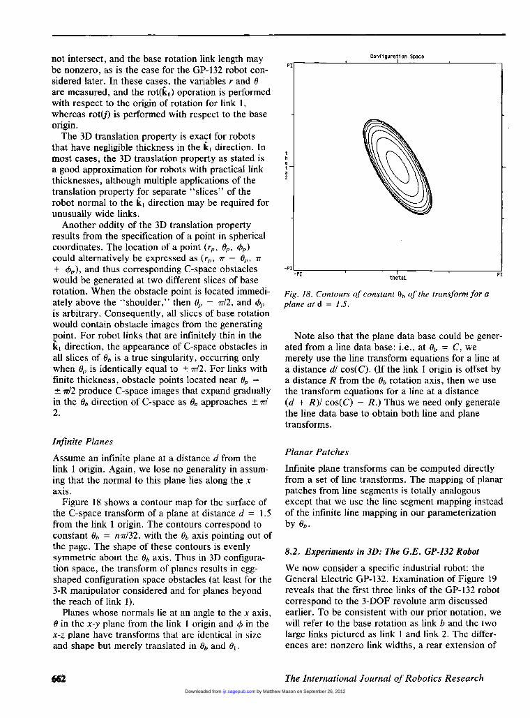
Figure 18 shows a contour map for the surface ofthe C-space transform of a plane at distance d = 1.5from the link 1 origin. The contours correspond toconstant Ob = n-ir/32, with the Ob axis pointing out ofthe page. The shape of these contours is evenlysymmetric about the Ob axis. Thus in 3D configura-tion space, the transform of planes results in egg-shaped configuration space obstacles (at least for the3-R manipulator considered and for planes beyondthe reach of link 1).

Planes whose normals lie at an angle to the x axis,0 in the x-y plane from the link 1 origin and 0 in thex-z plane have transforms that are identical in sizeand shape but merely translated in Ob and 01.

Fig. 18. Contours of constant eb of the transform for aplane at d = 1.5.

Note also that the plane data base could be gener-ated from a line data base: i.e., at Ob = C, wemerely use the line transform equations for a line ata distance d/ cos(C). (If the link I origin is offset bya distance R from the Ob rotation axis, then we usethe transform equations for a line at a distance(d + R)/ cos(C) - R.) Thus we need only generatethe line data base to obtain both line and planetransforms.

Planar Patches

Infinite plane transforms can be computed directlyfrom a set of line transforms. The mapping of planarpatches from line segments is totally analogousexcept that we use the line segment mapping insteadof the infinite line mapping in our parameterizationby 0b .

8.2. Experiments in 3D: The G.E. GP-132 Robot

We now consider a specific industrial robot: theGeneral Electric GP-132. Examination of Figure 19reveals that the first three links of the GP-132 robot

correspond to the 3-DOF revolute arm discussedearlier. To be consistent with our prior notation, wewill refer to the base rotation as link b and the two

large links pictured as link 1 and link 2. The differ-ences are: nonzero link widths, a rear extension of



663

Fig. 19. The GP-132 manipulator.

link 2, and joint limits. It should also be noted that

the B6 and 01 rotation axes are nonintersecting(therefore distance measurements are from the link 1origin).We will refer to the forward extension of link 2 as

link2,r,,, and the backward extension as link2bark’ Thelength of link 1 is 0.8 m; link2fronr is 1.185 m long;link2bark’ 0.85 m. The offset from the 8b axis to thelink 1 origin is 0.3 m.The first three links of the GP-132 are limited in

their rotation. The range of the base rotation is 300°.The ranges for link 1 and link 2 are 110° and 120°,respectively:

where 01 is measured from the horizontal, and 62is measured relative to link 1. Note that the planarR - R portion link1-link2 is one-handed.We define the &dquo;static&dquo; C-space of the GP-132 as

the transform of those obstacles that we do not

expect will ever change, such as joint limits, therobot’s own body, and the floor. For these obsta-cles, the forbidden poses of 01 and 02 are identicalfor all values of 0b . The static C-space of the GP-132is shown in Figure 20. The black regions are forbid-den. In this and the later figures, the C-space for theGP-132 is shown for constant B6 within the ranges

Fig. 20. The static C-space of the GP-132.

for link 1 and link 2 given above. The C-space isalso discretized, which we will discuss further.The general properties of C-space obstacles dis-

cussed throughout this article apply specifically tothe GP-132. Because the GP-132 has nonzero link

Fig. 21. GP-132 C-space transform for a point at d = 1.2,one slice.



664

Fig. 22. GP-132 C-space transform for a line at d = 1.2,one slice.

widths, even point transformations forbid wholeranges of 6~ for a given 01. The transform for a pointat a distance of 1.2 m is shown in Figure 21. Thetransform for a line at the same distance is given inFigure 22.

Fig. 23. One slice of GP-132 C-space, static plus ladder.

Point and line data bases for link 1, link2,,.,,,,,,, andlink2back were computed. The density of these databases was 1 cm-i.e., the transforms for points andlines at increments of 4 d = 1.0 cm were stored.The transforms of complex obstacles in the work

space can be built up from our point and line databases. Figure 23 shows one slice (constant 0b) of theC-space for the GP-132 with a ladder in its workspace. The thin regions of free space between obsta-cles correspond to those configurations where theGP-132 can maneuver link 2 between rungs of theladder.

9. Implementation Considerations andResults

The chief focus of this article and the novelty of itscontribution is the introduction of properties, repre-sentation, and algorithms that lead to dramaticincreases in the speed of configuration space trans-formations. Our experimental results show that withour techniques, useful speed and resolution of con-figuration space transforms can be obtained in threedimensions with commonly available computingpower. Experimental considerations and results arereported here for the experimental planar arm andfor the G.E. GP-132 industrial robot.

9.1. Discretized Configuration Space

Obstacles in C-space may be approximated analyt-ically (e.g., in terms of enclosing polygons, ellipses,or parallelepipeds) (Brady et al. 1982; Chen andVidyasagar 1988; Nguyen 1984, respectively). In ourapproach, we utilize a discretization of the C-space(Brooks and Lozano-Perez 1985; Lozano-Perez1987; Warren 1987).Two-dimensional C-space is discretized into a rec-

tangular array of pixels; three-dimensional C-spaceis discretized into a three-dimensional array of vox-els. Generically, we will refer to the C-space discre-tizations (pixels or voxels) as C-space bins or simplybins. We will refer to two-dimensional arrays of con-

stant 0b as slices.Discretized C-space can be built from the analytic

expressions or constructed from empirical measure-ments by &dquo;turning on&dquo; a bin if it contains any por-tion of the C-space obstacle. The discretized C-space used for the experimental planar arm was a128 x 128 array, resulting in an angular resolutionof 2.8I~.The discretized C-space used for the GP-132 was

a 128 x 128 x 128 array representing the allowableranges of joint motions. Thus there were 128 Bb



665

slices. This discretization results in bin sizes of0.86°, 0.94°, and 2.34° in 01, B2, and 8h, respectively.

9.2. Data Base Memory Requirements

By choosing a set of coordinates that takes advan-tage of the translation property, it is possible tocompute C-space transforms efficiently using ahybrid of analytic and table lookup evaluations. Thecomputationally intensive phase of C-space trans-forms may be precomputed and tabulated in reduceddimensionality. Such tabulations comprise our database of C-space elemental transforms.We have utilized two separate approaches to stor-

ing precomputed obstacle transformations. For theexperimental planar arm (Newman 1987b), 2D trans-formation results were stored as boundary descrip-tions. Boundaries of computed C-space obstacleswere approximated by bounding polygons (typicallynonconvex) and stored as linked lists of vertex coor-dinates. In this compact representation, the entirepoint-transform data base was stored in 84 coordi-nate pairs. Details of the boundary description tech-nique may be found in Newman (1987b).For the GP-132 robot, the data base of elemental

transforms consisted of the discretized C-spaceobstacles themselves (along the x-axis only).Although such a storage format permits rapid con-struction of C-space obstacles, the memory require-ments in 3D space are demanding. To compress thestored data, image coding techniques of ruu-lengthcoding (Horn 1986) and image following (Zuech1988) were used.

Details of the data compression may be found inBranicky (1990). Obstacle data bases for the GP-132robot were computed and stored in compressedform, comprising 123 and 36 kilobytes for the pointand line transforms, respectively. Storage of uncom-pressed bits would have required 2351 kilobytes perdata base. Total memory storage was cut from 4702to 159 kilobytes, a memory savings of a factor ofalmost 30.

9~.3. Speed of Transformations

Experiments in rapid computation of C-space obsta-cles were performed for both the experimentalplanar arm in two dimensions and the G.E. GP-132robot in three dimensions. In each case, the rate oftransformations depends on how cluttered the workspace is. Using our constructive geometry approach,the speed of transformations is a linear function ofthe number of primitives to be transformed. The

transformation process invites parallel processing,though we report only on single-processor results.

In experiments with the planar arm in 2D space,12-vertex polygonal approximations of circularobstacles were computed in real time for a 128 x128 discretization of C-space. The computer usedwas an MC68020-based single-board computer run-ning at 16.7 MHz. Configuration space maps werestored in off-board RAM, which was accessed via aVMEbusl backplane. The code was written in C lan-guage. In implementation for moving circular obsta-cles, erasing an obstacle, recomputing the obstacleboundaries, discretizing the boundaries, and comput-ing and storing edge normal information was exe-cuted in the worst case at 33 Hz per obstacle. Atthese rates, the planar arm was effective at avoidingcollisions in relatively complex dynamic environ-ments. Illustrative performance is shown in Newman(1988).Although the C-space transformation rate was

suitable for the 2D case, greater efficiency wasneeded for adequate performance in 3D space. Inour 3D implementation for the G.E. GP-132 robot,we obtained greater computational efficiency at theexpense of greater memory storage requirements.With data compression, though, the data base stor-age requirement for line and point obstacles wasonly 159 K bytes. Using a single 20-MHz MC68020-based computer, transformation of point or planeobstacles was achieved at speeds of 200 Hz perslice. The number of slices affected by any onepoint or line was usually small but always less than77. Thus the worst-case transformation rate for a

point or line was better than 2 Hz. Experiments aredocumented on videotape, available through New-man (1989).Based on our measurements, current conventional

computing hardware in a multiprocessor systemshould be capable of useful C-space transformationrates in 3D space that exceed camera frame rates.

10. Summary and ConclusionsThis presentation has introduced novel concepts thathave resulted in experimentally verified dramaticimprovements in the rapid computation of obstaclesin configuration space. The contributions includederivation of general properties of the nature of con-figuration space transformations; specification of anintermediate coordinate frame that permits highlyefficient computations; and the proposition of a con-

1. VMEbus is a trademark of Motorola. The VMEbus specifica-tion is equivalent to the IEEE 1014 and IEC 821 BUS standards.



666

structive geometry approach to computing complextransforms from the superposition of simpler, effi-cient transforms.

Key to the development is the definition of ele-mental building blocks that are easily transformedfrom work space to configuration space and may beused in superposition to model more complexshapes. Efficient transformation of these elements ispossible through a hybrid analytic/tabulated functionapproach. Tabulation of complex computations ismade possible through judicious choice of a refer-ence frame that permits dimensional reduction bycasting the transformation computation as a separa-ble function.

Experimental results are reported, verifying thevalidity and efficiency of the approach in 2D and 3Dspace. To our knowledge, this work represents byfar the fastest computation of configuration spaceobstacles yet achieved.

AcknowledgmentsThis work was partially supported by Philips Labo-ratories, North American Philips Corp.; by theNational Institute of Standards and Technologyunder grant no. 60NANB9D0934; and by the Cleve-land Advanced Manufacturing Program. Their sup-port is gratefully acknowledged.

References

Asada, H., and Slotine, J. J. E. 1986. Robot Analysis andControl. New York: John Wiley & Sons.

Boyse, J. W. 1979. Interference detection among solidsand surfaces. Communications ACM 22(1):3-9.

Brady, M., Hollerbach, J. M., Johnson, T. J., Lozano-Pérez, T., and Mason, M. T. 1982. Basics of robotmotion planning and control. In Robot Motion. Cam-bridge, MA: The MIT Press, pp. 1-50.

Branicky, M. S. 1990. Efficient Configuration SpaceTransforms for Real-Time Robotic Reflexes. Master’sthesis. Case Western Reserve University, Departmentof Electrical Engineering and Applied Physics, Cleve-land, Ohio.

Branicky, M. S., and Newman, W. S. 1990. Rapid compu-tation of configuration-space obstacles. Proceedings ofthe IEEE International Conference on Robotics andAutomation.

Brooks, R. A. 1983a. Planning collision-free motions forpick-and-place operations. Int. J. Robot. Res. 2(4):19-44.

Brooks, R. A. 1983b. Solving the find-path problem bygood representation of free space. IEEE Trans. Sys.Man Cybernet. SMC-13(3):190-197.

Brooks, R. A., and Lozano-Pérez, T. 1985. A subdivisionalgorithm in configuration space for findpath with rota-

tion. IEEE Trans. Sys. Man Cybernet. SMC-15(2):224-233.

Canny, J. 1986. Collision detection for moving polyhedra.IEEE Trans. Pattern Analysis Machine IntelligencePAMI-8(2):200-209.

Chen, Y. C., and Vidyasagar, M. 1988. Optimal trajectoryplanning for planar n-link revolute manipulators in thepresence of obstacles. Proceedings of the IEEE Interna-tional Conference on Robotics and Automation, pp.202-208.

Donald, B. R. 1987. A search algorithm for motion plan-ning with six degrees of freedom. Artificial Intelligence31:295-353.

Erdman, M., and Lozano-Pérez, T. 1986. On multiplemoving objects. Proceedings of the IEEE InternationalConference on Robotics and Automation, pp. 1419-1424.

Faverjon, B., and Tournassoud, P. 1987. A local basedapproach for path planning of manipulators with a highnumber of degrees of freedom. Proceedings of the IEEEInternational Conference on Robotics and Automation,pp. 1152-1159.

Herman, M. 1986. Fast, three-dimensional, collision-freemotion planning. Proceedings of the IEEE InternationalConference on Robotics and Automation, pp. 1056-1063.

Hopcroft, J., and Wilfong, G. 1986. Motion of objects incontact. Int. J. Robot. Res. 4(4):32-46.

Horn, B. K. 1986. Robot Vision. MIT Electrical Engineer-ing and Computer Science Series. Cambridge, MA: TheMIT Press.

Khatib, O. 1986. Real-time obstacle avoidance for manipu-lators and mobile robots. Int. J. Robot. Res. 5(1):90-98.

Korein, J. U. 1985. A Geometric Investigation of Reach.An ACM Distinguished Dissertation 1984. Cambridge,MA: The MIT Press.

Lozano-Pérez, T. 1981. Automatic planning of manipula-tor transfer movements. IEEE Trans. Sys. Man Cyber-net. SMC-11(10):681-698.

Lozano-Pérez, T. 1983. Spatial planning: A configurationspace approach. IEEE Trans. Computers C-32(2):108-120.

Lozano-Pérez, T. 1987. A simple motion-planning algo-rithm for general robotic manipulators. IEEE J. Robot.Automat. RA-3(3):224-238.

Lozano-Pérez, T., et al. 1987 (March). Handey: A robotsystem that recognizes, plans, and manipulates. Pro-ceedings of the IEEE International Conference onRobotics and Automation, pp. 843-849.

Lozano-Pérez, T., and Wesley, M. A. 1979. An algorithmfor planning collision-free paths among polyhedralobstacles. Communications ACM 22(10):560-570.

Lumelsky, V. J. 1987. Effect of kinematics on motionplanning for planar robot arms moving amidst unknownobstacles. IEEE J. Robot. Automat. RA-3(3):207-223.

Lumelsky, V. J., and Stepanov, A. A. 1986. Dynamicpath planning for a mobile automaton with limited infor-mation on the environment. IEEE Trans. Auto. Control

AC-31(11): 1058-1063.



667

Lumelsky, V., and Sun, K. 1987. Gross motion planningfor a simple 3D articulated robot arm moving amidstunknown arbitrarily shaped obstacles. Proceedings ofthe IEEE International Conference on Robotics andAutomation, pp. 1929-1934.

Maddila, S. R. 1986. Decomposition algorithm for movinga ladder among rectangular obstacles. Proceedings ofthe IEEE International Conference on Robotics andAutomation, pp. 1413-1418.

Meyer, W., and Benedict, P. 1988 (April). Path planningand the geometry of joint space obstacles. Proceedingsof the IEEE International Conference on Robotics andAutomation, pp. 215-219.

Newman, W. S. 1987a. High speed robot control andobstacle avoidance using dynamic potential functions.Proceedings of the IEEE International Conference onRobotics and Automation, pp. 14-24.

Newman, W. S. 1987b. High-Speed Robot Control inComplex Environments. Ph.D. thesis. MassachusettsInstitute of Technology, Department of MechanicalEngineering, Cambridge, Massachusetts.

Newman, W. S. 1988. High-Speed Robot Control withAutomatic Collision Avoidance. Video tape TR-89-138.Center for Automation and Intelligent SystemsResearch, Case Western Reserve University, Cleveland,Ohio.

Newman, W. S. 1989. Recent Advances in Robot ControlResearch at Case Western Reserve University. Videotape TR-89-139. Center for Automation and IntelligentSystems Research, Case Western Reserve University,Cleveland, Ohio.

Nguyen, V. D. 1984. The Find-Path Problem in the Plane.A.I. Memo 760, Artificial Intelligence Laboratory, Mas-sachusetts Institute of Technology, Cambridge, Massa-chusetts.

Noborio, H., Naniwa, T., and Arimoto, S. 1989. A feasi-ble motion-planning algorithm for a mobile robot on aquadtree representation. Proceedings of the IEEE Inter-national Conference on Robotics and Automation, pp.327-332.

Oommen, B. J., and Reichstein, 1. 1986. On translatingellipses amidst elliptic obstacles. Proceedings of theIEEE International Conference on Robotics and Auto-mation, pp. 1755-1759.

Red, W. E., and Truong-Cao, H. V. 1985. Configurationmaps for robot path planning in two dimensions. Trans.ASME 107:292-298.

Rimon, E., and Koditschek, D. E. 1989. The constructionof analytic diffeomorphisms for exact robot navigationon star worlds. Proceedings of the IEEE InternationalConference on Robotics and Automation, pp. 21-26.

Udupa, S. 1977. Collision detection and avoidance incomputer controlled manipulators. Ph.D. thesis. Califor-nia Institute of Technology, Department of ElectricalEngineering, Pasadena, California.

Warren, C. W. 1987. Robot Path Planning in the Presenceof Stationary and Moving Obstacles. Ph.D. thesis.Texas A&M University, Department of MechanicalEngineering, College Station, Texas.

Weeks, J. R. 1985. The Shape of Space. Pure and AppliedMathematics, vol. 96. New York: Marcel Dekker.

Wilfong, G. T. 1988. Motion planning for an autonomousvehicle. Proceedings of the IEEE International Confer-ence on Robotics and Automation, pp. 529-533.

Yap, C. K. 1984. How to move a chair through a door.IEEE J. Robot. Automat. RA-3(3):172-181.

Zuech, N. 1988. Applying Machine Vision. New York:John Wiley & Sons.



Documents

The International Journal of Robotics Research … · Additional services and information for The International Journal of Robotics Research ... machine controllers is ... Many studies