The International Journal of Robotics Research ... · ... Visual servoing is a well-known method that ... and Courbon et al. (2009),

http://ijr.sagepub.com/Robotics Research

The International Journal of

http://ijr.sagepub.com/content/early/2012/09/03/0278364912460413The online version of this article can be found at:

DOI: 10.1177/0278364912460413

published online 4 September 2012The International Journal of Robotics ResearchAndrea Cherubini and Francois Chaumette

Visual Navigation of a Mobile Robot with Laser-based Collision Avoidance

Published by:

http://www.sagepublications.com

On behalf of:

Multimedia Archives

can be found at:The International Journal of Robotics ResearchAdditional services and information for

http://ijr.sagepub.com/cgi/alertsEmail Alerts:

http://ijr.sagepub.com/subscriptionsSubscriptions:

http://www.sagepub.com/journalsReprints.navReprints:

http://www.sagepub.com/journalsPermissions.navPermissions:

What is This?

- Sep 4, 2012OnlineFirst Version of Record >>

at INRIA RENNES on September 6, 2012ijr.sagepub.comDownloaded from

http://ijr.sagepub.com/

http://ijr.sagepub.com/content/early/2012/09/03/0278364912460413

http://www.sagepublications.com

http://www.ijrr.org/

http://ijr.sagepub.com/cgi/alerts

http://ijr.sagepub.com/subscriptions

http://www.sagepub.com/journalsReprints.nav

http://www.sagepub.com/journalsPermissions.nav

http://ijr.sagepub.com/content/early/2012/09/03/0278364912460413.full.pdf

http://online.sagepub.com/site/sphelp/vorhelp.xhtml


Visual navigation of a mobile robot withlaser-based collision avoidance

The International Journal ofRobotics Research0(0) 1–17© The Author(s) 2012Reprints and permission:sagepub.co.uk/journalsPermissions.navDOI: 10.1177/0278364912460413ijr.sagepub.com

Andrea Cherubini1,2 and François Chaumette1

AbstractIn this paper, we propose and validate a framework for visual navigation with collision avoidance for a wheeled mobilerobot. Visual navigation consists of following a path, represented as an ordered set of key images, which have beenacquired by an on-board camera in a teaching phase. While following such a path, the robot is able to avoid obstacleswhich were not present during teaching, and which are sensed by an on-board range scanner. Our control schemeguarantees that obstacle avoidance and navigation are achieved simultaneously. In fact, in the presence of obstacles,the camera pan angle is actuated to maintain scene visibility while the robot circumnavigates the obstacle. The risk ofcollision and the eventual avoiding behaviour are determined using a tentacle-based approach. The framework can alsodeal with unavoidable obstacles, which make the robot decelerate and eventually stop. Simulated and real experimentsshow that with our method, the vehicle can navigate along a visual path while avoiding collisions.

Keywordsvision-based navigation, visual servoing, collision avoidance, integration of vision with other sensors

1. Introduction

A great amount of robotics research focuses on vehicleguidance, with the ultimate goal of automatically reproduc-ing the tasks usually performed by human drivers (Buehleret al., 2008; Zhang et al., 2008; Nunes et al., 2009; Broggiet al., 2010). In many recent works, information from visualsensors is used for localization Guerrero et al. (2008);Scaramuzza and Siegwart (2008) or for navigation (Bonin-Font et al., 2008; López-Nicolás et al., 2010). In the case ofautonomous navigation, an important task is obstacle avoid-ance, which consists of either generating a collision-freetrajectory to the goal (Minguez et al., 2008), or deceleratingto prevent collision when bypassing is impossible (Wadaet al., 2009). Most obstacle avoidance techniques, partic-ularly those that use motion planning (Latombe, 1991),rely on knowledge of a global and accurate map of theenvironment and obstacles.

Instead of utilizing such a global model of the envi-ronment, which would infringe the perception to actionparadigm (Sciavicco and Siciliano, 2000), we propose aframework for obstacle avoidance with simultaneous exe-cution of a visual servoing task (Chaumette and Hutchin-son, 2006). Visual servoing is a well-known method thatuses vision data directly in the control loop, and that has

been applied on mobile robots in many works Mariottiniet al. (2007); Allibert et al. (2008); Becerra et al. (2011);López-Nicolás and Sagüés (2011). For example, Mariot-tini et al. (2007) exploited the epipolar geometry to drivea non-holonomic robot to a desired configuration. A sim-ilar approach is presented by Becerra et al. (2011), wherethe singularities are dealt with more efficiently. The sameauthors achieved vision-based pose stabilization using astate observer in López-Nicolás and Sagüés (2011). Tra-jectory tracking is tackled by Allibert et al. (2008) byintegrating differential flatness and predictive control.

The visual task that we focus on is appearance-basednavigation, which has been the target of our research ofŠegvic et al. (2008), Cherubini et al. (2009) and Diosiet al. (2011). In the framework that we have developed inthe past,1 the path is a topological graph, represented by adatabase of ordered key images. In contrast with other simi-lar approaches, such as that of Booij et al. (2007), our graph

1INRIA Rennes - Bretagne Atlantique, IRISA, Rennes, France2LIRMM - Université de Montpellier 2 CNRS, Montpellier, France

Corresponding author:Andrea Cherubini, LIRMM - Université de Montpellier 2 CNRS, 161 RueAda, 34392 Montpellier, France.Email: [email protected]



2 The International Journal of Robotics Research 0(0)

does not contain forks. Furthermore, as opposed to Royeret al. (2007), Goedemé et al. (2007), Zhang and Kleeman(2009), Fontanelli et al. (2009) and Courbon et al. (2009),we do not use the robot pose for navigating along the path.Instead, our task is purely image-based (as in the approachof Becerra et al. (2010)), and it is divided into a seriesof subtasks, each consisting of driving the robot towardsthe next key image in the database. More importantly, tothe best of the authors’ knowledge, appearance-based nav-igation frameworks have never been extended to take intoaccount obstacles.

Obstacle avoidance has been integrated into many model-based navigation schemes. Yan et al. (2003) used a rangefinder and monocular vision to enable navigation in anoffice environment. The desired trajectory is deformed toavoid sensed obstacles in the work of Lamiraux et al.(2004). Ohya et al. (2008) use a model-based vision systemwith retroactive position correction. Simultaneous obsta-cle avoidance and path following are presented by Lapierreet al. (2007), where the geometry of the path (a curve onthe ground) is perfectly known. In the approach of Leeet al. (2010), obstacles are circumnavigated while follow-ing a path; the radius of the obstacles (assumed cylindrical)is known a priori. In practice, all of these methods are basedon the environment 3D model, including, for example, wallsand doors, or on the path geometry. In contrast, we proposea navigation scheme which does not require an environmentor obstacle model.

One of the most common techniques for model-freeobstacle avoidance is the potential field method, origi-nally introduced by Khatib (1985). The gap between globalpath planning and real-time sensor-based control has beenclosed with an elastic band (Quinlan and Khatib, 1993), adeformable collision-free path, whose initial shape is gener-ated by a planner, and then deformed in real time, accordingto the sensed data. Similarly, in the work of Bonnafouset al. (2001) and Von Hundelshausen et al. (2008), a setof trajectories (arcs of circles or ‘tentacles’) is evaluatedfor navigating. However, in the work of Bonnafous et al.(2001), a sophisticated probabilistic elevation map is used,and the selection of the optimal tentacle is based on its riskand interest, which both require accurate pose estimation.Similarly, in Von Hundelshausen et al. (2008), the trajectorycomputation relies on GPS way points, hence once more onthe robot pose.

Here, we focus on this problem: a wheeled vehicle,equipped with an actuated pinhole camera and with aforward-looking range scanner, must follow a visual pathrepresented by key images, without colliding with theground obstacles. The camera detects the features requiredfor navigating, while the scanner senses the obstacles (incontrast with other works, such as that of Kato et al. (2002),only one sensor is used to detect the obstacles). In thissense, our work is similar to that of Folio and Cadenat(2006), where redundancy enables reactive obstacle avoid-ance, without requiring any 3D model. A robot is redundant

when it has more degrees of freedom (DOFs) than thoserequired for the primary task; then, a secondary task canalso be executed. In the work of Folio and Cadenat (2006),the two tasks are respectively visual servoing and obsta-cle avoidance. However, there are various differences withthat work. First, we show that the redundancy approach isnot necessary, since we design the two tasks so that theyare independent. Second, we can guarantee asymptotic sta-bility of the visual task at all times, in the presence ofnon-occluding obstacles. Moreover, our controller is com-pact, and the transitions between safe and unsafe contextsis operated only for obstacle avoidance, while in the workof Folio and Cadenat (2006), three controllers are needed,and the transitions are more complex. This compactnessleads to smoothness of the robot behaviour. Finally, Folioand Cadenat (2006) considered a positioning task in indoorenvironments, whereas we aim at continuous navigation onlong outdoor paths.

Let us summarize the other major contributions of ourwork. An important contribution is that our approach ismerely appearance-based, hence simple and flexible: theonly information required is the database of key images,and no model of the environment or obstacles is neces-sary. Hence, there is no need for sensor data fusion norplanning, which can be computationally costly, and requiresprecise calibration of the camera/scanner pair. We guaran-tee that the robot will never collide in the case of static,detectable obstacles (in the worse cases, it will simply stop).We also prove that our control law is always well-defined,and that it does not present any local minima. To the bestof the authors’ knowledge, this is the first time that obstacleavoidance and visual navigation merged directly at the con-trol level (without the need for sophisticated planning) arevalidated in real outdoor urban experiments.

The framework that we present here is inspired from thatdesigned and validated in our previous work (Cherubiniand Chaumette, 2011). However, many modifications havebeen applied, in order to adapt that controller to the realworld. First, for obstacle avoidance, we have replaced clas-sical potential fields with a new tentacle-based techniqueinspired by Bonnafous et al. (2001) and Von Hundelshausenet al. (2008), which is perfectly suitable for appearance-based tasks, such as visual navigation. In contrast with thoseworks, our approach does not require the robot pose, andexploits the robot geometric and kinematic characteristics(this aspect will be detailed later in the paper). A detailedcomparison between the potential field and the tentacletechniques is given in Cherubini et al. (2012). In that work,we showed that with tentacles, smoother control inputs aregenerated, higher velocities can be applied, and only dan-gerous obstacles are taken into account. In summary, thenew approach is more robust and efficient than its prede-cessor. A second modification with respect to Cherubiniand Chaumette (2011) concerns the design of the transla-tional velocity, which has been changed to improve visualtracking and avoid undesired deceleration in the presence of



Cherubini and Chaumette 3

x d

CURRENT IMAGE I

KEY IMAGES I1 N

Visual Navigation

NEXT KEY IMAGE I dy

Ox

v

Zc X

C

Y

Xc

Y c

Z R

ϕ

ϕ

ω

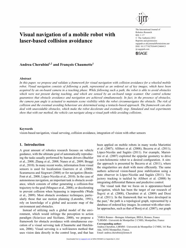
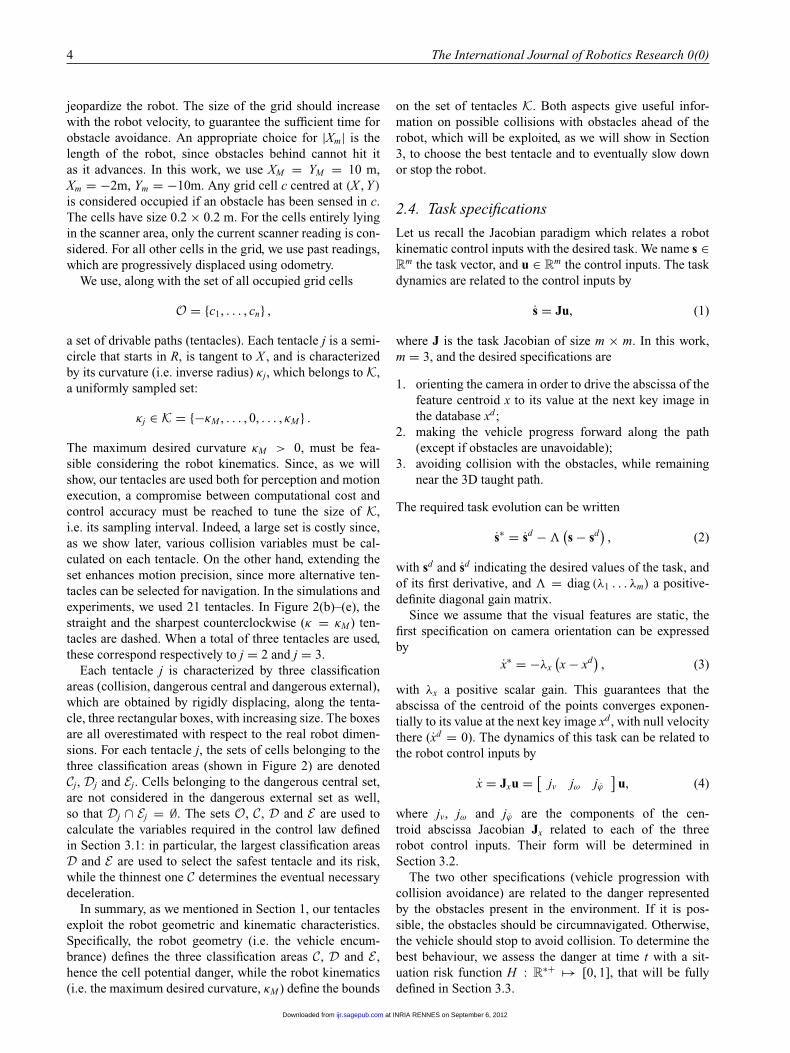
Fig. 1. General definitions. Left: top view of the robot (rectangle),equipped with an actuated camera (triangle); the robot and cameraframe (respectively, FR and FC ) are shown. Right: database ofthe key images, with current and next key images emphasized;the image frame FI is also shown, as well as the visual features(circles) and their centroid (cross).

non-dangerous obstacles. Another important contributionof the present work is that, in contrast with the tentacle-based approaches designed in Von Hundelshausen et al.(2008) and Bonnafous et al. (2001), our method does notrequire the robot pose. Finally, the present article reportsexperiments, which, for the first time in the field of visualnavigation with obstacle avoidance, have been carried outin real-life, unpredictable urban environments.

The article is organized as follows. In Section 2, thecharacteristics of our problem (visual path following withsimultaneous obstacle avoidance) are presented. The con-trol law is presented in full detail in Section 3, and a shortdiscussion is carried out in Section 4. Simulated and realexperimental results are presented respectively in Sections5 and 6, and summarized in the conclusion.

2. Problem definition

2.1. General definitions

The reader is referred to Figure 1. We define the robotframe FR (R, X , Y ) (R is the robot centre of rotation), imageframe FI( O, x, y) (O is the image centre) and camera frameFC (C, Xc, Yc, Zc) (C is the optical centre). The robot controlinputs are

u = (v, ω, ϕ) .

These are, respectively, the translational and angular veloc-ities of the vehicle, and the camera pan angular velocity. Weuse the normalized perspective camera model:

x = Xc

Zc, y = Yc

Zc.

We assume that the camera pan angle is bounded: |ϕ| ≤π2 , and that C belongs to the camera pan rotation axis, andto the robot sagittal plane (i.e. the plane orthogonal to theground through X ). We also assume that the path can befollowed with continuous v (t) > 0. This ensures safety,since only obstacles in front of the robot can be detected byour range scanner.

c1

23

c3

c4

33

13

c2 13

R

(e)

(b) (a)

c1

R

12

XM X

Ym YM Xm

c1

c2

Y c3

c4

R

c1

c3 R

12

(c)

c1

c2

R

X

Y

23

c3

c4

(d) δ

δ

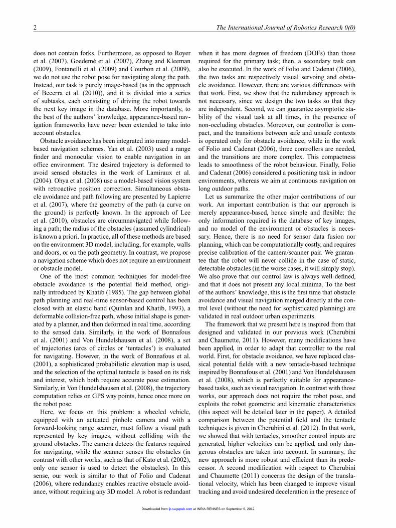
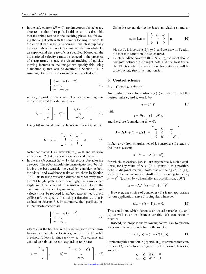
Fig. 2. Obstacle models with four occupied cells c1, . . . , c4. (a)Occupancy grid, straight (b, c) and sharpest counterclockwise (d,e) tentacles (dashed). When a total of three tentacles are used, thestraight and sharpest counterclockwise are characterized, respec-tively, by index j = 2 and j = 3. For these two tentacles, wehave drawn: classification areas (collision Cj, dangerous centralDj, dangerous external Ej), corresponding boxes and delimitingarcs of circle, and cell risk and collision distances (�ij, δij). Fortentacle j = 3 in the bottom right, we have also drawn the tentaclecentre (cross) and the ray of cell c1, denoted by �13.

2.2. Visual path following

The path that the robot must follow is represented as adatabase of ordered key images, such that successive pairscontain some common static visual features (points). First,the vehicle is manually driven along a taught path, with thecamera pointing forward (ϕ = 0), and all of the imagesare saved. Afterwards, a subset (database) of N key imagesI1, . . . , IN representing the path (Figure 1, right) is selected.Then, during autonomous navigation, the current image,denoted I , is compared with the next key image in thedatabase, Id ∈ {I1, . . . , IN }, and a relative pose estimationbetween I and Id is used to check when the robot passes thepose where Id was acquired.

For key image selection, as well as visual point detectionand tracking, we use the algorithm presented in Royer et al.(2007). The output of this algorithm, which is used by ourcontroller, is the set of points visible both in I and Id . Then,navigation consists of driving the robot forward, while I isdriven towards Id . We maximize similarity between I andId using only the abscissa x of the centroid of the pointsmatched on I and Id . When Id has been passed, the nextimage in the set becomes the desired one, and so on, untilIN is reached.

2.3. Obstacle representation

Along with the visual path following problem, we considerobstacles which are on the path, but not in the database,and sensed by the range scanner in a plane parallel to theground. We use the occupancy grid in Figure 2(a): it islinked to FR, with cell sides parallel to X and Y . Its lon-gitudinal and lateral extensions are limited (Xm ≤ X ≤ XM

and Ym ≤ Y ≤ YM ), to ignore obstacles that are too far to




jeopardize the robot. The size of the grid should increasewith the robot velocity, to guarantee the sufficient time forobstacle avoidance. An appropriate choice for |Xm| is thelength of the robot, since obstacles behind cannot hit itas it advances. In this work, we use XM = YM = 10 m,Xm = −2m, Ym = −10m. Any grid cell c centred at (X , Y )

is considered occupied if an obstacle has been sensed in c.The cells have size 0.2 × 0.2 m. For the cells entirely lyingin the scanner area, only the current scanner reading is con-sidered. For all other cells in the grid, we use past readings,which are progressively displaced using odometry.

We use, along with the set of all occupied grid cells

O = {c1, . . . , cn} ,

a set of drivable paths (tentacles). Each tentacle j is a semi-circle that starts in R, is tangent to X , and is characterizedby its curvature (i.e. inverse radius) κj, which belongs to K,a uniformly sampled set:

κj ∈ K = {−κM , . . . , 0, . . . , κM } .

The maximum desired curvature κM > 0, must be fea-sible considering the robot kinematics. Since, as we willshow, our tentacles are used both for perception and motionexecution, a compromise between computational cost andcontrol accuracy must be reached to tune the size of K,i.e. its sampling interval. Indeed, a large set is costly since,as we show later, various collision variables must be cal-culated on each tentacle. On the other hand, extending theset enhances motion precision, since more alternative ten-tacles can be selected for navigation. In the simulations andexperiments, we used 21 tentacles. In Figure 2(b)–(e), thestraight and the sharpest counterclockwise (κ = κM ) ten-tacles are dashed. When a total of three tentacles are used,these correspond respectively to j = 2 and j = 3.

Each tentacle j is characterized by three classificationareas (collision, dangerous central and dangerous external),which are obtained by rigidly displacing, along the tenta-cle, three rectangular boxes, with increasing size. The boxesare all overestimated with respect to the real robot dimen-sions. For each tentacle j, the sets of cells belonging to thethree classification areas (shown in Figure 2) are denotedCj, Dj and Ej. Cells belonging to the dangerous central set,are not considered in the dangerous external set as well,so that Dj ∩ Ej = ∅. The sets O, C, D and E are used tocalculate the variables required in the control law definedin Section 3.1: in particular, the largest classification areasD and E are used to select the safest tentacle and its risk,while the thinnest one C determines the eventual necessarydeceleration.

In summary, as we mentioned in Section 1, our tentaclesexploit the robot geometric and kinematic characteristics.Specifically, the robot geometry (i.e. the vehicle encum-brance) defines the three classification areas C, D and E ,hence the cell potential danger, while the robot kinematics(i.e. the maximum desired curvature, κM ) define the bounds

on the set of tentacles K. Both aspects give useful infor-mation on possible collisions with obstacles ahead of therobot, which will be exploited, as we will show in Section3, to choose the best tentacle and to eventually slow downor stop the robot.

2.4. Task specifications

Let us recall the Jacobian paradigm which relates a robotkinematic control inputs with the desired task. We name s ∈R

m the task vector, and u ∈ Rm the control inputs. The task

dynamics are related to the control inputs by

s = Ju, (1)

where J is the task Jacobian of size m × m. In this work,m = 3, and the desired specifications are

1. orienting the camera in order to drive the abscissa of thefeature centroid x to its value at the next key image inthe database xd;

2. making the vehicle progress forward along the path(except if obstacles are unavoidable);

3. avoiding collision with the obstacles, while remainingnear the 3D taught path.

The required task evolution can be written

s∗ = sd − (s − sd

), (2)

with sd and sd indicating the desired values of the task, andof its first derivative, and = diag (λ1 . . . λm) a positive-definite diagonal gain matrix.

Since we assume that the visual features are static, thefirst specification on camera orientation can be expressedby

x∗ = −λx

(x − xd

), (3)

with λx a positive scalar gain. This guarantees that theabscissa of the centroid of the points converges exponen-tially to its value at the next key image xd , with null velocitythere (xd = 0). The dynamics of this task can be related tothe robot control inputs by

x = Jxu = [jv jω jϕ

]u, (4)

where jv, jω and jϕ are the components of the cen-troid abscissa Jacobian Jx related to each of the threerobot control inputs. Their form will be determined inSection 3.2.

The two other specifications (vehicle progression withcollision avoidance) are related to the danger representedby the obstacles present in the environment. If it is pos-sible, the obstacles should be circumnavigated. Otherwise,the vehicle should stop to avoid collision. To determine thebest behaviour, we assess the danger at time t with a sit-uation risk function H : R

∗+ �→ [0, 1], that will be fullydefined in Section 3.3.




• In the safe context (H = 0), no dangerous obstacles aredetected on the robot path. In this case, it is desirablethat the robot acts as in the teaching phase, i.e. follow-ing the taught path with the camera looking forward. Ifthe current pan angle ϕ is non-null, which is typicallythe case when the robot has just avoided an obstacle,an exponential decrease of ϕ is specified. Moreover, thetranslational velocity v must be reduced in the presenceof sharp turns, to ease the visual tracking of quicklymoving features in the image; we specify this usinga function vs that will be detailed in Section 3.4. Insummary, the specifications in the safe context are

⎧⎨⎩

x = −λx

(x − xd

)v = vs

ϕ = −λϕϕ

, (5)

with λϕ a positive scalar gain. The corresponding cur-rent and desired task dynamics are

ss =⎡⎣

xvϕ

⎤⎦ , s∗

s =⎡⎣

−λx

(x − xd

)vs

−λϕϕ

⎤⎦ . (6)

Using (4) we can derive the Jacobian relating ss and u:

ss = Jsu =⎡⎣

jv jω jϕ1 0 00 0 1

⎤⎦ u. (7)

Note that matrix Js is invertible if jω = 0, and we showin Section 3.2 that this condition is indeed ensured.

• In the unsafe context (H = 1), dangerous obstacles aredetected. The robot should circumnavigate them by fol-lowing the best tentacle (selected by considering boththe visual and avoidance tasks as we show in Section3.3). This heading variation drives the robot away fromthe 3D taught path. Correspondingly, the camera panangle must be actuated to maintain visibility of thedatabase features, i.e. to guarantee (3). The translationalvelocity must be reduced for safety reasons (i.e. to avoidcollisions); we specify this using a function vu, that isdefined in Section 3.5. In summary, the specificationsin the unsafe context are

⎧⎨⎩

x = −λx

(x − xd

)v = vu

ω = κbvu

, (8)

where κb is the best tentacle curvature, so that the trans-lational and angular velocities guarantee that the robotprecisely follows it, since ω/v = κb. The current anddesired task dynamics corresponding to (8) are

su =⎡⎣

xvω

⎤⎦ , s∗

u =⎡⎣

−λx

(x − xd

)vu

κbvu

⎤⎦ . (9)

Using (4) we can derive the Jacobian relating su and u:

su = Juu =⎡⎣

jv jω jϕ1 0 00 1 0

⎤⎦ u. (10)

Matrix Ju is invertible if jϕ = 0, and we show in Section3.2 that this condition is also ensured.

• In intermediate contexts (0 < H < 1), the robot shouldnavigate between the taught path and the best tenta-cle. The transition between these two extremes will bedriven by situation risk function H .

3. Control scheme

3.1. General scheme

An intuitive choice for controlling (1) in order to fulfill thedesired tasks su and ss would be

u = J−1s∗ (11)

withs = Hsu + (1 − H) ss

and therefore (considering H = 0):

J = HJu + (1 − H) Js =⎡⎣

jv jω jϕ1 0 00 H 1 − H

⎤⎦ .

In fact, away from singularities of J, controller (11) leads tothe linear system:

s − sd = −(s − sd

)

for which, as desired,(sd , sd

)are exponentially stable equi-

libria, for any value of H ∈ [0, 1] (since is a positive-definite diagonal matrix). Note that replacing (2) in (11),leads to the well-known controller for following trajectorysd = sd (t), given by (Chaumette and Hutchinson, 2007)

u = −J−1( s − sd) +J−1sd .

However, the choice of controller (11) is not appropriatefor our application, since J is singular whenever

Hjϕ + (H − 1) jω = 0. (12)

This condition, which depends on visual variables (jϕ andjω) as well as on an obstacle variable (H), can occur inpractice.

Instead, we propose the following control law to guaran-tee a smooth transition between the inputs:

u = HJ−1u s∗

u + (1 − H) J−1s s∗

s . (13)

Replacing this equation in (7) and (10), guarantees that con-troller (13) leads to convergence to the desired tasks (5)and (8):

ss = s∗s if H = 0

su = s∗u if H = 1




and that, in these cases, the desired states are glob-ally asymptotically stable for the closed loop system. InSection 4, we show that global asymptotic stability of thevisual task is also guaranteed in the intermediate cases(0 < H < 1).

In the following, we define the variables introduced inSection 2.4. We show how to derive the centroid abscissaJacobian Jx, the situation risk function H , the best tentaclealong with its curvature κb, and the translational velocitiesin the safe and unsafe context (vs and vu, respectively).

3.2. Jacobian of the centroid abscissa

We will hereby derive the components of Jx introducedin (4). Let us define v = (vc, ωc) the camera velocity,expressed in FC . Since we have assumed that the featuresare static, the dynamics of x can be related to v by

x = Lxv

where Lx is the interaction matrix of x (Chaumette andHutchinson, 2006). In the case of a point of depth Zc, itis given by (Chaumette and Hutchinson, 2006)

Lx =[

− 1Zc

0 xZc

xy −1 − x2 y]

. (14)

In theory, since we consider the centroid and not a physi-cal point, we should not use (14) for the interaction matrix,but the exact and more complex form given in Tahri andChaumette (2005). However, using (14) provides a suffi-ciently accurate approximation (Cherubini et al., 2009). Italso has the strong advantage that it is not necessary to esti-mate the depth of all points, using techniques such as thosedescribed by Davison et al. (2007), De Luca et al. (2008)and Durand et al. (2010). Only an approximation of Zc,i.e. one scalar, is sufficient. In practice, we set a constantfixed value. This strategy has proved successful for visualnavigation in Cherubini et al. (2009).

For the robot model that we are considering, the cameravelocity v can be expressed as a function of u by using thegeometric model:

v =C TRu

with:

CTR =

⎡⎢⎢⎢⎢⎢⎢⎣

sin ϕ −X C cos ϕ 00 0 0

cos ϕ X C sin ϕ 00 0 00 −1 −10 0 0

⎤⎥⎥⎥⎥⎥⎥⎦

.

In this matrix, X C is the abscissa of the optical centre C inthe robot frame FR. This parameter is specific of the robotplatform. Since C belongs to the robot sagittal plane, andsince the robot is constrained on the ground plane, this isthe only coordinate of C in FR required for visual servoing.

Then, multiplying Lx by CTR, we obtain the componentsof Jx:

jv = − sin ϕ+x cos ϕ

Zc

jω = X C(cos ϕ+x sin ϕ)

Zc+ 1 + x2

jϕ = 1 + x2.

(15)

From (15) it is clear that jϕ ≥ 1 ∀x ∈ R; hence, Ju is neversingular (see (10)). Furthermore, it is possible to ensure thatjω = 0, so that Js is also invertible (see (7)). In fact, in (15)

we can guarantee that jω = 0, by setting Zc > X C

2 in the Jx

components. Indeed, condition jω = 0 is equivalent to

X C (cos ϕ + x sin ϕ)

Zc+ 1 + x2 = 0. (16)

Since |ϕ| ≤ π2 : cos ϕ + x sin ϕ ≥ −x, ∀x ∈ R. Hence, a

sufficient condition for (16) is

x2 − X C

Zcx + 1 > 0,

which occurs ∀x ∈ R when X C/Zc < 2. In practice, thiscondition can be guaranteed, since X C is an invariant char-acteristic of the robot platform, and Zc is a tunable controlparameter, which can be set to a value greater than X C/2. Inaddition, the value of X C on most robots platforms is usu-ally smaller than 1 m, which is much less than the scenedepth in outdoor environments. In Cherubini et al. (2009),we have shown that overestimating Zc does not jeopardizenavigation.

On the other hand, we can infer from (15) that the sin-gularity of controller (11), expressed by (12) can occur fre-quently. For example, whenever Zc is large, yielding jϕ ≈jω, and concurrently H ≈ 0.5, J becomes singular. Thisconfirms the great interest in choosing control scheme (13),

which is always well defined if Zc > X C

2 .

3.3. Situation risk function and best tentacle

To derive the situation risk function H used in (13), we firstcalculate a candidate risk function Hj ∈ [0, 1] for each ten-tacle, as will be explained below. Each Hj is derived fromthe risk distance of all occupied cells in the dangerous areas.

This distance is denoted �ij ≥ 0 for each ci ∈ O ∩(Dj ∪ Ej

). For occupied cells in the central set Dj, �ij is

the distance that the middle boundary box would coveralong tentacle j before touching the cell centre. For occu-pied cells in the external set, only a subset Ej is taken intoaccount: Ej ⊆ O ∩ Ej. This subset contains only cells whichreduce the clearance in the tentacle normal direction. Foreach external occupied cell, we denote �ij the ray starting atthe tentacle centre and passing through ci. Cell ci is addedto Ej if and only if, in Dj ∪ Ej, there is at least an occu-pied cell crossed by �ij on the other side of the tentacle. Inthe example of Figure 2(e), O ∩ E3 = {c1, c3, c4}, whereasE3 = {c1, c3}. Cell c4 is not considered dangerous, sinceit is external, and does not have a counterpart on the other




side of the tentacle. Then, for cells in Ej, �ij is the sum oftwo terms: the distance from the centre of ci to its normalprojection on the perimeter of the dangerous central area,and the distance that the middle boundary box would coveralong tentacle j before reaching the normal projection. Thederivation of �ij is illustrated, in Figure 2, for four occupiedcells. Note that for a given cell, �ij may have different val-ues (or even be undefined) according to the tentacle that isconsidered.

When all risk distances on tentacle j are calculated, wecompute �j as their minimum:

�j = infci∈(O∩Dj)∪Ej

�ij.

If(O ∩ Dj

) ∪ Ej ≡ ∅, �j = ∞. In the example of Figure2, �2 = �12 and �3 = �33. Obviously, overestimating thebounding box sizes leads to more conservative �j.

We then use �j and two hand-tuned thresholds �d and�s (0 < �d < �s) to design the tentacle risk function:

Hj=

⎧⎪⎪⎨⎪⎪⎩

0 if �j ≥�s

12

[1 + tanh

(1

�j−�d+ 1

�j−�s

)]if �d <�j <�s

1 if �j ≤�d .(17)

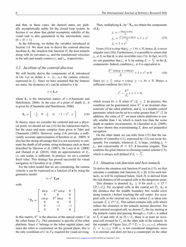
Note that Hj smoothly varies from 0, when the dangerouscells associated with tentacle j (if any) are far, to 1, whenthey are near. If Hj = 0, the tentacle is tagged as clear.In practice, threshold �s must be set to the risk distancefor which the context ceases to be safe (H becomes greaterthan 0), so that the robot starts to leave the taught (occu-pied) path. On the other hand, �d must be tuned as the riskdistance for which the context becomes unsafe (H = 1),so that the robot follows the best tentacle to circumnavigatethe obstacle. In our work, we used the values �s = 6 m and�d = 4.5 m. The risk function Hj corresponding to thesevalues is plotted in Figure 3.

The Hj of all tentacles are then compared, in order todetermine H in (13). Initially, we calculate the path curva-ture κ = ω/v ∈ R that the robot would follow if there wereno obstacles. Replacing H = 0 in (13), it is

κ = [λx

(xd − x

) − jvvs + λϕ jϕϕ]/jωvs,

which is always well defined, since jω = 0 and we have setvs > 0. We obviously constrain κ to the interval of feasiblecurvatures [−κM , κM ]. Then, we derive the two neighboursof κ among all of the existing tentacle curvatures:

κn, κnn ∈ K such that κ ∈ [κn, κnn) .

Let κn be the nearest, i.e. the curvature of the tentacle thatbest approximates the safe path.2 We denote it as the visualtask tentacle. The situation risk function Hv of that tentacleis then obtained by linear interpolation of its neighbours:

Hv = (Hnn − Hn) κ + Hnκnn − Hnnκn

κnn − κn. (18)

1

Hj

j

5.02.5 7.5 10�

Fig. 3. Risk Hj as a function of the tentacle risk distance �j (m)when �s = 6 m and �d = 4.5 m.

(a)

c1

c2 c1

(c) (d) 1

c1

c1

c2

(b)

�

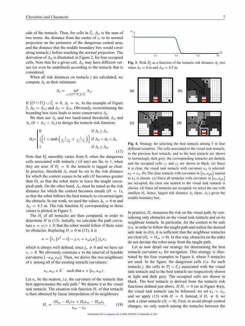
Fig. 4. Strategy for selecting the best tentacle among 5 in fourdifferent scenarios. The cells associated to the visual task tentacle,to the previous best tentacle, and to the best tentacle are shownin increasingly dark grey; the corresponding tentacles are dashed,and the occupied cells c1 and c2 are shown in black. (a) Sinceit is clear, the visual task tentacle with curvature κn is selected:κb = κn. (b) The clear tentacle with curvature in

[κn, κpb

]nearest

to κn is chosen. (c) Since all tentacles with curvature in[κn, κpb

]are occupied, the clear one nearest to the visual task tentacle ischosen. (d) Since all tentacles are occupied, we select the one withsmallest Hj, hence, largest risk distance �j (here, �1) given themiddle boundary box.

In practice, Hv measures the risk on the visual path, by con-sidering only obstacles on the visual task tentacle and on itsneighbour tentacle. In particular, for the context to be safe(i.e. in order to follow the taught path and realize the desiredsafe task in (6)), it is sufficient that the neighbour tentaclesare clear (Hn = Hnn = 0). In this way, obstacles on the sidesdo not deviate the robot away from the taught path.

Let us now detail our strategy for determining the besttentacle curvature κb for navigation. This strategy is illus-trated by the four examples in Figure 4, where 5 tentaclesare used. In the figure, the dangerous cells (i.e. for eachtentacle j, the cells in Dj ∪ Ej) associated with the visualtask tentacle and to the best tentacle are respectively shownin light and dark grey. The occupied cells are shown inblack. The best tentacle is derived from the tentacle riskfunctions defined just above. If Hv = 0 (as in Figure 4(a)),the visual task tentacle can be followed: we set κb = κn,and we apply (13) with H = 0. Instead, if Hv = 0, weseek a clear tentacle (Hj = 0). First, to avoid abrupt controlchanges, we only search among the tentacles between the




visual task one and the best one at the previous iteration,3

denoted by κpb, and mid-grey in the figure. If many clearones are present, the nearest to the visual task tentacle ischosen, as in Figure 4(b). If none of the tentacles withcurvature in

[κn, κpb

]is clear, we search among the oth-

ers. Again, the best tentacle will be the clear one that isclosest to κn and, in case of ambiguity, the one closest toκnn. If a clear tentacle has been found (as in Figure 4(c)),we select it and set H = 0. Instead, if no tentacle in Kis clear, the one with minimum Hj calculated using (17)is chosen, and H is set equal to that Hj. In the exampleof Figure 4(d), tentacle 1 is chosen and we set H = H1,since �1 = sup{�1, . . . , �5}, hence H1 = inf{H1, . . . , H5}.Eventual ambiguities are again solved first with the distancefrom κn, then from κnn.

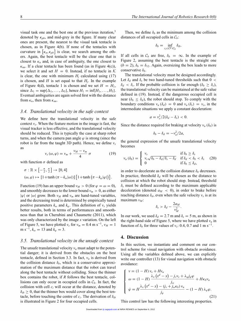
3.4. Translational velocity in the safe context

We define here the translational velocity in the safecontext vs. When the feature motion in the image is fast, thevisual tracker is less effective, and the translational velocityshould be reduced. This is typically the case at sharp robotturns, and when the camera pan angle ϕ is strong (since therobot is far from the taught 3D path). Hence, we define vs

as

vs (ω, ϕ) = vm + vM − vm

4σ (19)

with function σ defined as

σ : R × [−π2 , π

2

] → [0, 4]

(ω, ϕ) �→ [1+tanh (π−kω|ω|)] [1+tanh

(π−kϕ |ϕ|)] .

Function (19) has an upper bound vM > 0 (for ϕ = ω = 0),and smoothly decreases to the lower bound vm > 0, as either|ϕ| or |ω| grow. Both vM and vm are hand-tuned variables,and the decreasing trend is determined by empirically tunedpositive parameters kω and kϕ . This definition of vs yieldsbetter results, both in terms of performances and smooth-ness than that in Cherubini and Chaumette (2011), whichwas only characterized by the image x variation. On the leftof Figure 5, we have plotted vs for vm = 0.4 m s−1, vM = 1m s−1, kω = 13 and kϕ = 3.

3.5. Translational velocity in the unsafe context

The unsafe translational velocity vu must adapt to the poten-tial danger; it is derived from the obstacles on the besttentacle, defined in Section 3.3. In fact, vu is derived fromthe collision distance δb, which is a conservative approxi-mation of the maximum distance that the robot can travelalong the best tentacle without colliding. Since the thinnerbox contains the robot, if R follows the best tentacle, col-lisions can only occur in occupied cells in Cb. In fact, thecollision with cell ci will occur at the distance, denoted byδib ≥ 0, that the thinner box would cover along the best ten-tacle, before touching the centre of ci. The derivation of δib

is illustrated in Figure 2 for four occupied cells.

Then, we define δb as the minimum among the collisiondistances of all occupied cells in Cb:

δb = infci∈O∩Cb

δib.

If all cells in Cb are free, δb = ∞. In the example ofFigure 2, assuming the best tentacle is the straight one(b = 2), δb = δ12. Again, oversizing the box leads to moreconservative δb.

The translational velocity must be designed accordingly.Let δd and δs be two hand-tuned thresholds such that 0 <

δd < δs. If the probable collision is far enough (δb ≥ δs),the translational velocity can be maintained at the safe valuedefined in (19). Instead, if the dangerous occupied cell isnear (δb ≤ δd), the robot should stop. To comply with theboundary conditions vu (δd) = 0 and vu (δs) = vs, in theintermediate situations we apply a constant deceleration:

a = v2s /2(δd − δs) < 0.

Since the distance required for braking at velocity vu (δb) is

δb − δd = −v2u/2a,

the general expression of the unsafe translational velocitybecomes

vu (δb) =⎧⎨⎩

vs if δb ≥ δs

vs√

δb − δd/δs − δd if δd < δb < δs

0 if δb ≤ δd ,(20)

in order to decelerate as the collision distance δb decreases.In practice, threshold δd will be chosen as the distance tocollision at which the robot should stop. Instead, thresholdδs must be defined according to the maximum applicabledeceleration (denoted aM < 0), in order to brake beforereaching distance δd , even when the safe velocity vs is at itsmaximum vM :

δs > δd − 2aM

v2M

.

In our work, we used δd = 2.7 m and δs = 5 m, as shown inthe right-hand side of Figure 5, where we have plotted vu infunction of δb for three values of vs: 0.4, 0.7 and 1 m s−1.

4. Discussion

In this section, we instantiate and comment on our con-trol scheme for visual navigation with obstacle avoidance.Using all the variables defined above, we can explicitlywrite our controller (13) for visual navigation with obstacleavoidance:⎧⎪⎪⎪⎪⎨⎪⎪⎪⎪⎩

v = (1 − H) vs + Hvu

ω = (1 − H)λx

(xd − x

) − jvvs + λϕ jϕϕ

jω+ Hκbvu

ϕ = Hλx

(xd − x

) − (jv + jωκb) vu

jϕ− (1 − H) λϕϕ.

(21)This control law has the following interesting properties.




- /2- /2 - /2 - /2- /2

- /2 -0.3 0

0.3

vs

0.7

1.0

-1.5

1.5

0

vu

1.0

5.02.70.4

0.7

0.4

vs=1

vs=0.7

vs=0.4

ϕ

δb

ω

Fig. 5. Left: safe translational velocity vs (m s−1) as a function of ω (rad s−1) and ϕ (rad). Right: unsafe translational velocityvu (m s−1) as a function of δb (m) for three different values of vs.

1. In the safe context (H = 0), Equation (21) becomes⎧⎪⎪⎨⎪⎪⎩

v = vs

ω = λx

(xd − x

) − jvvs + λϕ jϕϕ

jωϕ = −λϕϕ.

(22)

In Section 3.1, we proved that this controller guaran-tees global asymptotic stability of the safe task s∗

s . Asin Cherubini et al. (2009) and Diosi et al. (2011), whereobstacles were not considered, the image error is con-trolled only by ω, which also compensates the centroiddisplacements due to v and to ϕ through the imageJacobian components (15), to fulfil the visual task (3).The two remaining specifications in (5), instead, areachieved by inputs v and ϕ: the translational velocity isregulated to improve tracking according to (19), whilethe camera is driven forward, to ϕ = 0. Note that, toobtain H = 0 with the tentacle approach, it is sufficientthat the neighbour tentacles are clear (Hn = Hnn = 0),whereas in the potential field approach used by Cheru-bini and Chaumette (2011), even a single occupied cellwould generate H > 0. Thus, one advantage of the newapproach is that only obstacles on the visual path aretaken into account.

2. In the unsafe context (H = 1), Equation (21) becomes⎧⎪⎪⎨⎪⎪⎩

v = vu

ω = κbvu

ϕ = λx

(xd − x

) − (jv + jωκb) vu

jϕ.

(23)

In Section 3.1, we proved that this controller guaran-tees global asymptotic stability of the unsafe task s∗

u. Inthis case, the visual task (3) is executed by ϕ, while thetwo other specifications are ensured by the two otherDOFs: the translational velocity is reduced (and evenzeroed to v = vu = 0 for very near obstacles such thatδb ≤ δd), while the angular velocity makes the robotfollow the best tentacle (ω/v = κb). Note that, sinceno 3D positioning sensor (e.g. GPS) is used, closing theloop on the best tentacle is not possible; however, evenif the robot slips (e.g. due to a flat tyre), at the follow-ing iterations tentacles with stronger curvature will be

selected to drive it towards the desired path, and so on.Finally, the camera velocity ϕ in (23) compensates therobot rotation, to keep the features in view.

3. In intermediate situations (0 < H < 1), the robot navi-gates between the taught path, and the best path consid-ering obstacles. The situation risk function H represent-ing the danger on the taught path, drives the transition,but not the speed. In fact, note that, for all H ∈ [0, 1],when δb ≥ δs: v = vs. Hence, a high velocity can beapplied if the path is clear up to δs (e.g. when navigatingbehind another vehicle).

4. Control law (21) guarantees that obstacle avoidance hasno effect on the visual task, which can be achieved forany H ∈ [0, 1]. Note that plugging the expressions of v,ω and ϕ from (21) into the visual task equation:

x = jvv + jωω + jϕ ϕ (24)

yields (3). Therefore, the desired state xd is globallyasymptotically stable for the closed-loop system, ∀H ∈[0, 1]. This is true even in the special case where v = 0.In fact, the robot stops and v becomes null, if and onlyif H = 1 and vu = 0, implying that ω = 0 and

ϕ = λx

(xd−x

)

jϕ, which allows realization of the visual

task. In summary, from a theoretical control viewpoint(i.e. without considering image processing nor field ofview or joint limits constraints), this proves that if atleast one point in Id is visible, the visual task of drivingthe centroid abscissa to xd will be achieved, even in thepresence of unavoidable obstacles. This strategy is veryuseful for recovery: since the camera stays focused onthe visual features, as soon as the path returns free, therobot can follow it again.

5. Controller (21) does not present local minima, i.e. non-desired state configurations for which u is null. In fact,when H < 1, u = 0 requires both vu and vs to be null,but this is impossible since from (19)), vs > vm > 0.Instead, when H = 1, it is clear from (23) that for u tobe null it is sufficient that xd − x = 0 and vu = 0. Thiscorresponds to null desired dynamics: s∗

u = 0 (see (9)).This task is satisfied, since plugging u = 0 into (10),yields precisely su = 0 = s∗

u.




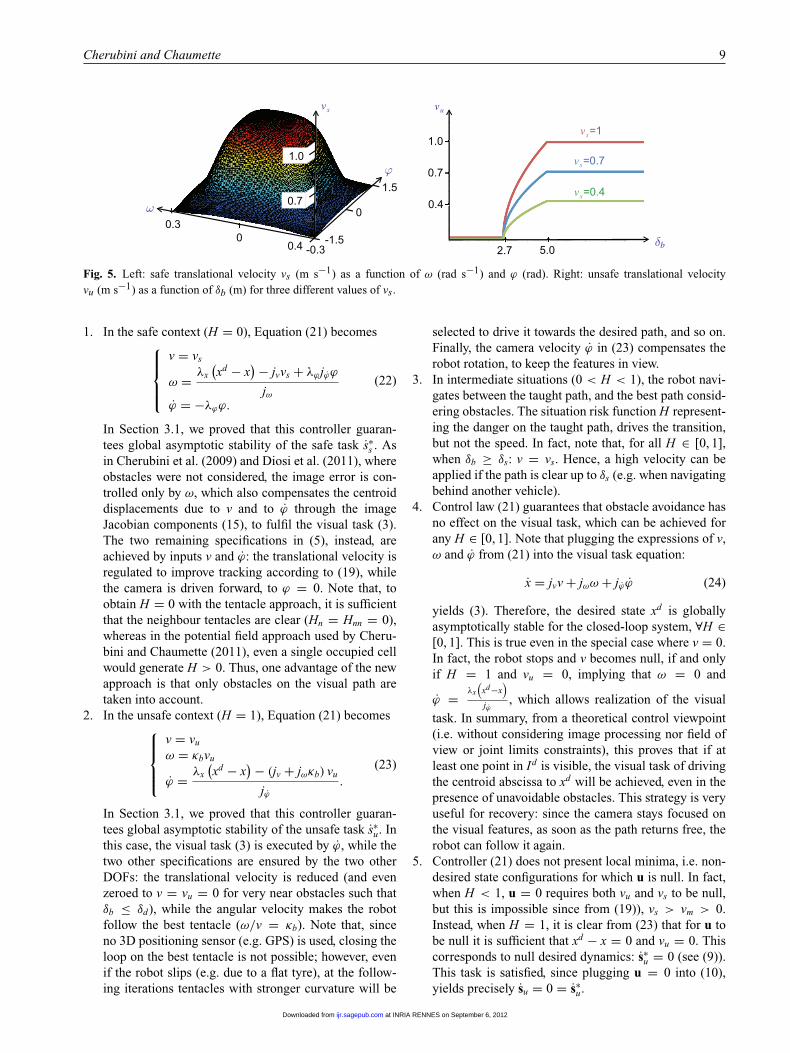
A B C D E F

Fig. 6. Six obstacle scenarios for replaying two taught paths (black) with the robot (rectangle): a straight segment (scenarios A to C),and a closed-loop followed in the clockwise sense (D to F). Visual features are represented by the spheres, the occupancy grid by therectangular area, and the replayed paths are drawn in grey.

6. If we tune the depth Zc to infinity in (15), jv = 0, andjϕ = jω = 1 + x2. Thus, control law (21) becomes

⎧⎪⎪⎪⎪⎨⎪⎪⎪⎪⎩

v = (1 − H) vs + Hvu

ω = (1 − H) λxxd − x

jω+ (1 − H) λϕϕ + Hκbvu

ϕ = Hλxxd − x

jω− (1 − H) λϕϕ + Hκbvu.

Note that, for small image error (x ≈ xd), ϕ ≈ −ω.In practice, the robot rotation is compensated for by thecamera pan rotation, which is an expected behaviour.

5. Simulations

In this section and in the following, we provide details ofthe simulated and real experiments that were used to vali-date our approach. Simulations are in the video shown inExtension 1.

For simulations, we made use of Webots,4 where wedesigned a car-like robot equipped with an actuated 320 ×240 pixels 70◦ field of view camera, and with a 110◦ scan-ner of range 15 m. Both sensors operate at 30 Hz. The visualfeatures, represented by spheres, are distributed randomlyin the environment, with depths with respect to the robotvarying from 0.1 to 100 m. The offset between R and C isX C = 0.7 m, and we set Zc = 15 m that meets the con-dition Zc > X C/2. We use 21 tentacles, with κM = 0.35m−1 (the robot maximum applicable curvature). For the sit-uation risk function, we use �s = 6 m and �d = 4.5 m.These parameters correspond to the design of H shown inFigure 3. The safe translational velocity is designed withvm = 0.4 m s−1, vM = 1 m s−1, κω = 13 and κϕ = 3, as inthe graph on the left-hand side of Figure 5. For the unsafetranslational velocity, we use δs = 5 m and δd = 2.7 m as onthe right-hand side of Figure 5 (top curve). The simulationswere helpful for tuning the control gains, in all experiments,to λx = 1 and λϕ = 0.5.

At first, no obstacle is present in the environment, andthe robot is driven along a taught path. Then, up to fiveobstacles are located, near and on the taught path, and therobot must replay the visual path, while avoiding them. Inaddition, the obstacles may partially occlude the features.

Although the sensors are noise-free, and feature matching isideal, these simulations allow validation of controller (21).

By displacing the obstacles, we have designed the sixscenarios shown in Figure 6. For scenarios A, B and C,the robot has been previously driven along a 30 m straightpath, and N = 8 key images have been acquired, whereasin scenarios D, E and F, the taught path is a closed loop oflength 75 m and N = 20 key images, which is followedin the clockwise sense. In all scenarios, the robot is able tonavigate without colliding, and this is done with the sameparameters. The metrics used to assess the experiments arethe image error with respect to the visual database x−xd (inpixels), averaged over the whole experiment and denoted e,and the distance, at the end of the experiment, from the final3D key pose (ε, in centimetres). The first metric e is use-ful to assess the controller accuracy in realizing the visualpath following task. The latter metric is less relevant, sincetask (3) is defined in the image space, and not in the posespace.

In all six scenarios, path following has been achieved,and in some cases, navigation was completed using onlythree image points. Obviously, this is possible in simula-tions, since feature detection is ideal: in the real case, whichincludes noise, three points may be insufficient. Some por-tions of the replayed paths, corresponding to the obstaclelocations, are far from the taught ones. However, these devi-ations would have been indispensable to avoid collisions,even with a pose-based control scheme. Let us detail therobot behaviour in the six scenarios:

• Scenario A: two walls, which were not present dur-ing teaching, are parallel to the path, and three boxesare placed in between. The first box is detected, andovertaken on the left. Then, the vehicle passes betweenthe second box and the left wall, and then overtakesthe third box on the right. Finally, the robot con-verges back to the path, and completes it. Although thewalls occlude features on the sides, the experiment issuccessful, with e = 5, and ε = 23.

• Scenario B: it is similar to scenario A, except that thereare no boxes, and that the left wall is shifted towardsthe right one, making the passage narrower towards theend. This makes the robot deviate in order to pass in thecentre of the passage. We obtain e = 6, ε = 18.




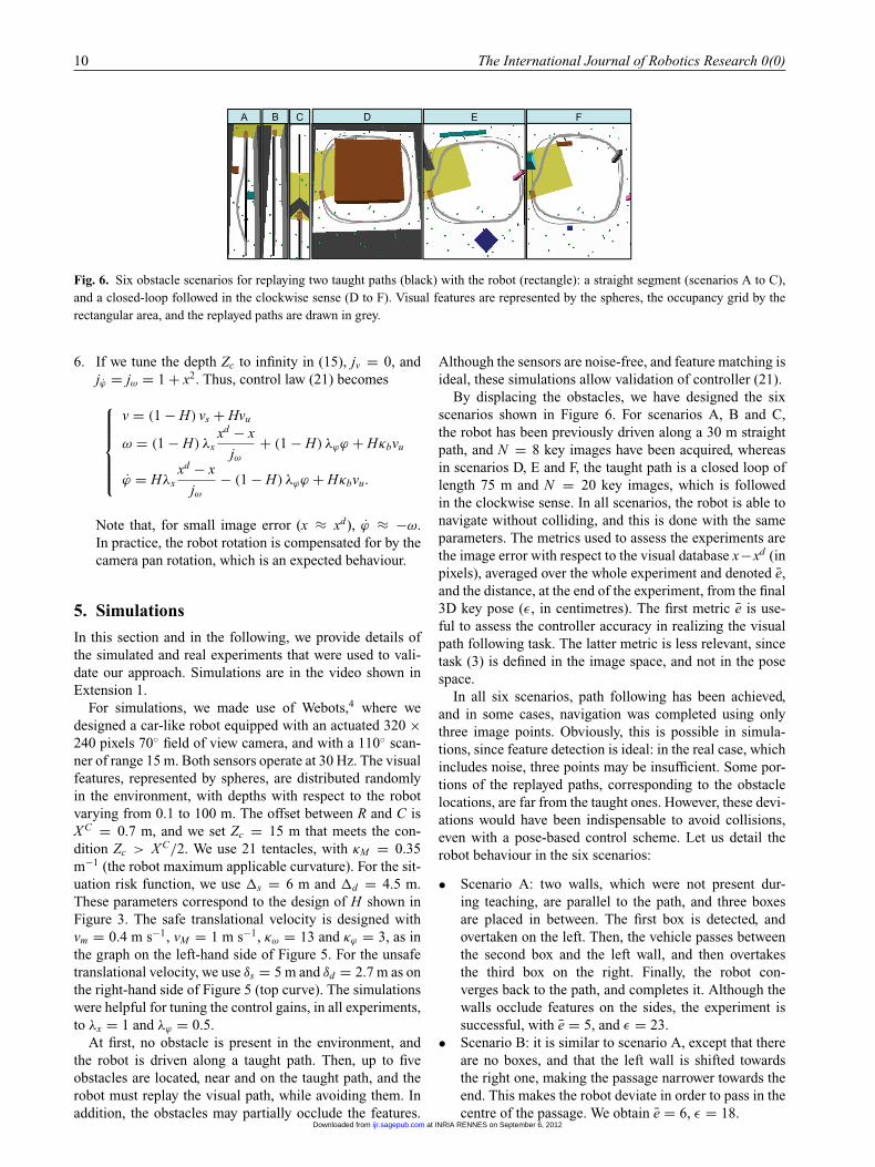
Fig. 7. Scenario A. For each of the five relevant iterations we show (top to bottom) the robot overtaking the first obstacle, the next keyimage, the current image and the occupancy grid.

• Scenario C: this scenario is designed to test the con-troller in the presence of unavoidable obstacles. Twowalls forming a corner, are located on the path. Thissoon makes all tentacles unsafe: �j ≤ �d| ∀j, yieldingH = 1. In addition, as the robot approaches the wall,the collision distance on the best tentacle δb decreases,and eventually becomes smaller than δd , to make vu = 0and stop the robot (see (23)). Although the path is notcompleted (making metric ε irrelevant), the collision isavoided, and e = 4 pixels. As proved in Section 4, con-vergence of the visual task (x = xd) is achieved, in spiteof u = 0. In particular, here, the centroid abscissa onthe third key image in the database is reached.

• Scenario D: high walls are present on both sides of thepath; this leads to important occlusions (less than 50%of the database features are visible), and to a consequentdrift from the taught path. Nevertheless, the final keyimage is reached, without collisions, and with e = 34and ε = 142. Although this metric is higher than in theprevious scenarios (since the path is longer and there arenumerous occlusions), it is still reasonably low.

• Scenario E: two obstacles are located on the path, andtwo others are near the path. The first obstacle is over-taken on the left, before avoiding the second one, alsoon the left. Then, the robot converges to the path andavoids the third obstacle on the right, before reachingthe final key image. We obtain e = 33 and ε = 74. Theexperiment shows one of the advantages of our tentacle-based approach: lateral data in the grid is ignored (con-sidering the fourth obstacle, would have made the robotcurve away from the path).

• Scenario F: here, the controller is assessed in a situa-tion where classical obstacle avoidance strategies (e.g.potential fields) often fail because of local minima.In fact, when detected, the first obstacle is centred onthe X axis and orthogonal to it. This may induce anambiguity, since occupancies are symmetric withrespect to X . However, the visual features distribution,and consequent visual task tentacle κn drive the robotto the right of the obstacle, which is thus avoided.We have repeated this experiment with 10 randomlygenerated visual feature distributions, and in all casesthe robot avoided the obstacle. The scenario involvesfour more obstacles, two of which are circumnavi-gated externally, and two on the inside. Here, e = 29and ε = 75.

In Figure 7, we show five stages of scenario A. In thisfigure, as well as later in Figures 12 and 14, the segmentslinking the current and next key image points are drawnin the current image. In the occupancy grid, the danger-ous cell sets associated with the visual task tentacle and tothe best tentacle (when different) are respectively shown ingrey and black, and two black segments indicate the scan-ner amplitude. Only cells that can activate H (i.e. cells atdistance � < �s) have been drawn. At the beginning of theexperiment (iteration 10), the visual features are driving therobot towards the first obstacle. When it is near enough, theobstacle triggers H (iteration 200), forcing the robot awayfrom the path towards the best tentacle, while the camerarotates clockwise to maintain feature visibility (iterations




0

-0.4

-0.25

1.0

0

0.6

0.25

6000

6000

0

1.0

6000

6000

0 6000

3000

3000

3000

1500

4500

4500

4500

4500

3000 4500

3000

0.4

-0.6

1500

1500

1500

1500

v

H iterations

iterations

iterations

iterations

iterations

ω

ϕ

ϕ

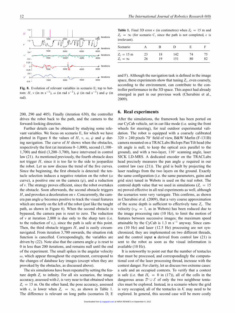
Fig. 8. Evolution of relevant variables in scenario E; top to bot-tom: H , v (in m s−1), ω (in rad s−1), ϕ (in rad s−1) and ϕ (inrad).

200, 290 and 405). Finally (iteration 630), the controllerdrives the robot back to the path, and the camera to theforward-looking direction.

Further details can be obtained by studying some rele-vant variables. We focus on scenario E, for which we haveplotted in Figure 8 the values of H , v, ω, ϕ and ϕ dur-ing navigation. The curve of H shows when the obstacles,respectively the first (at iterations 0–1,000), second (1,100–1,700) and third (3,200–3,700), have intervened in controllaw (21). As mentioned previously, the fourth obstacle doesnot trigger H , since it is too far to the side to jeopardizethe robot. Let us now discuss the trend of the five curves.Since the beginning, the first obstacle is detected: the ten-tacle selection induces a negative rotation on the robot (ωcurve), a positive one on the camera (ϕ), and a reductionof v. The strategy proves efficient, since the robot overtakesthe obstacle. Soon afterwards, the second obstacle triggersH , and provokes a deceleration on v. Concurrently, the cam-era pan angle ϕ becomes positive to track the visual featureswhich are mostly on the left of the robot (just like the taughtpath, as shown in Figure 6). When the second obstacle isbypassed, the camera pan is reset to zero. The reductionof v at iteration 2,800 is due only to the sharp turn (i.e.to the reduction of vs), since the path is safe at this point.Then, the third obstacle triggers H , and is easily circum-navigated. From iteration 3,700 onwards, the situation riskfunction is cancelled. Correspondingly, the variables aredriven by (22). Note also that the camera angle ϕ is reset to0 in less than 200 iterations, and remains null until the endof the experiment. The small spikes in the angular velocityω, which appear throughout the experiment, correspond tothe changes of database key images (except when they areprovoked by the obstacles, as discussed above).

The six simulations have been repeated by setting the fea-ture depth Zc to infinity. For all six scenarios, the imageaccuracy, assessed with e, is very near to that obtained whenZc = 15 m. On the other hand, the pose accuracy, assessedwith ε, is lower when Zc = ∞, as shown in Table 1.The difference is relevant on long paths (scenarios D, E

Table 1. Final 3D error ε (in centimetres) when Zc = 15 m andZc = ∞ (for scenario C, since the path is not completed, ε isirrelevant).

Scenario A B D E F

Zc = 15 m 23 18 142 74 75Zc = ∞ 26 19 151 80 82

and F). Although the navigation task is defined in the imagespace, these experiments show that tuning Zc, even coarsely,according to the environment, can contribute to the con-troller performance in the 3D space. This aspect had alreadyemerged in part in our previous work (Cherubini et al.,2009).

6. Real experiments

After the simulations, the framework has been ported onour CyCab vehicle, set in car-like mode (i.e. using the frontwheels for steering), for real outdoor experimental vali-dation. The robot is equipped with a coarsely calibrated320 × 240 pixels 70◦ field of view, B&W Marlin (F-131B)camera mounted on a TRACLabs Biclops Pan/Tilt head (thetilt angle is null, to keep the optical axis parallel to theground), and with a two-layer, 110◦ scanning angle, laserSICK LD-MRS. A dedicated encoder on the TRACLabshead precisely measures the pan angle ϕ required in ourcontrol law (see (21)). The grid is built by projecting thelaser readings from the two layers on the ground. Exactlythe same configuration (i.e. the same parameters, gains andgrid size) tuned in Webots is used on the real robot. Thecentroid depth value that we used in simulations (Zc = 15m) proved effective in all real experiments as well, althoughthe scenarios were very variegate. This confirms, as shownin Cherubini et al. (2009), that a very coarse approximationof the scene depth is sufficient to effectively tune Zc. Thevelocity (vM = 1, as in Webots) has been reduced due tothe image processing rate (10 Hz), to limit the motion offeatures between successive images; the maximum speedattainable by the CyCab is 1.3 m s−1 anyway. Since cam-era (10 Hz) and laser (12.5 Hz) processing are not syn-chronized, they are implemented on two different threads,and the control input u derived from control law (21) issent to the robot as soon as the visual information isavailable (10 Hz).

It is noteworthy to point out that the number of tentaclesthat must be processed, and correspondingly the computa-tional cost of the laser processing thread, increase with thecontext danger. For clarity, let us discuss two extreme cases:a safe and an occupied contexts. To verify that a contextis safe (i.e. that Hv = 0 in (17)), all of the cells in thedangerous areas D ∪ E of only the two neighbour tenta-cles must be explored. Instead, in a scenario where the gridis very occupied, all of the tentacles in K may need to beexplored. In general, this second case will be more costly




1.1

-0.5 45 15 30 60 75 time (s)

v H

ω

ϕ

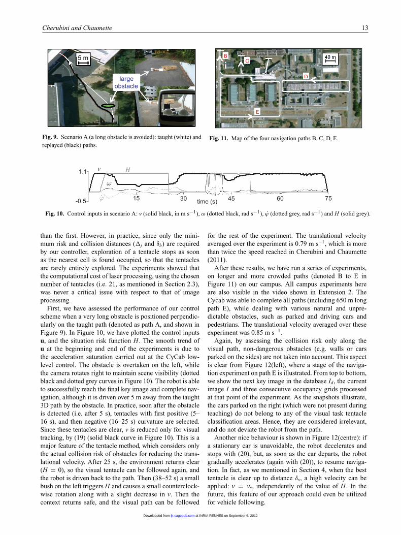
Fig. 10. Control inputs in scenario A: v (solid black, in m s−1), ω (dotted black, rad s−1), ϕ (dotted grey, rad s−1) and H (solid grey).

large obstacle

5 m 5 m

Fig. 9. Scenario A (a long obstacle is avoided): taught (white) andreplayed (black) paths.

than the first. However, in practice, since only the mini-mum risk and collision distances (�j and δb) are requiredby our controller, exploration of a tentacle stops as soonas the nearest cell is found occupied, so that the tentaclesare rarely entirely explored. The experiments showed thatthe computational cost of laser processing, using the chosennumber of tentacles (i.e. 21, as mentioned in Section 2.3),was never a critical issue with respect to that of imageprocessing.

First, we have assessed the performance of our controlscheme when a very long obstacle is positioned perpendic-ularly on the taught path (denoted as path A, and shown inFigure 9). In Figure 10, we have plotted the control inputsu, and the situation risk function H . The smooth trend ofu at the beginning and end of the experiments is due tothe acceleration saturation carried out at the CyCab low-level control. The obstacle is overtaken on the left, whilethe camera rotates right to maintain scene visibility (dottedblack and dotted grey curves in Figure 10). The robot is ableto successfully reach the final key image and complete nav-igation, although it is driven over 5 m away from the taught3D path by the obstacle. In practice, soon after the obstacleis detected (i.e. after 5 s), tentacles with first positive (5–16 s), and then negative (16–25 s) curvature are selected.Since these tentacles are clear, v is reduced only for visualtracking, by (19) (solid black curve in Figure 10). This is amajor feature of the tentacle method, which considers onlythe actual collision risk of obstacles for reducing the trans-lational velocity. After 25 s, the environment returns clear(H = 0), so the visual tentacle can be followed again, andthe robot is driven back to the path. Then (38–52 s) a smallbush on the left triggers H and causes a small counterclock-wise rotation along with a slight decrease in v. Then thecontext returns safe, and the visual path can be followed

Fig. 11. Map of the four navigation paths B, C, D, E.

for the rest of the experiment. The translational velocityaveraged over the experiment is 0.79 m s−1, which is morethan twice the speed reached in Cherubini and Chaumette(2011).

After these results, we have run a series of experiments,on longer and more crowded paths (denoted B to E inFigure 11) on our campus. All campus experiments hereare also visible in the video shown in Extension 2. TheCycab was able to complete all paths (including 650 m longpath E), while dealing with various natural and unpre-dictable obstacles, such as parked and driving cars andpedestrians. The translational velocity averaged over theseexperiment was 0.85 m s−1.

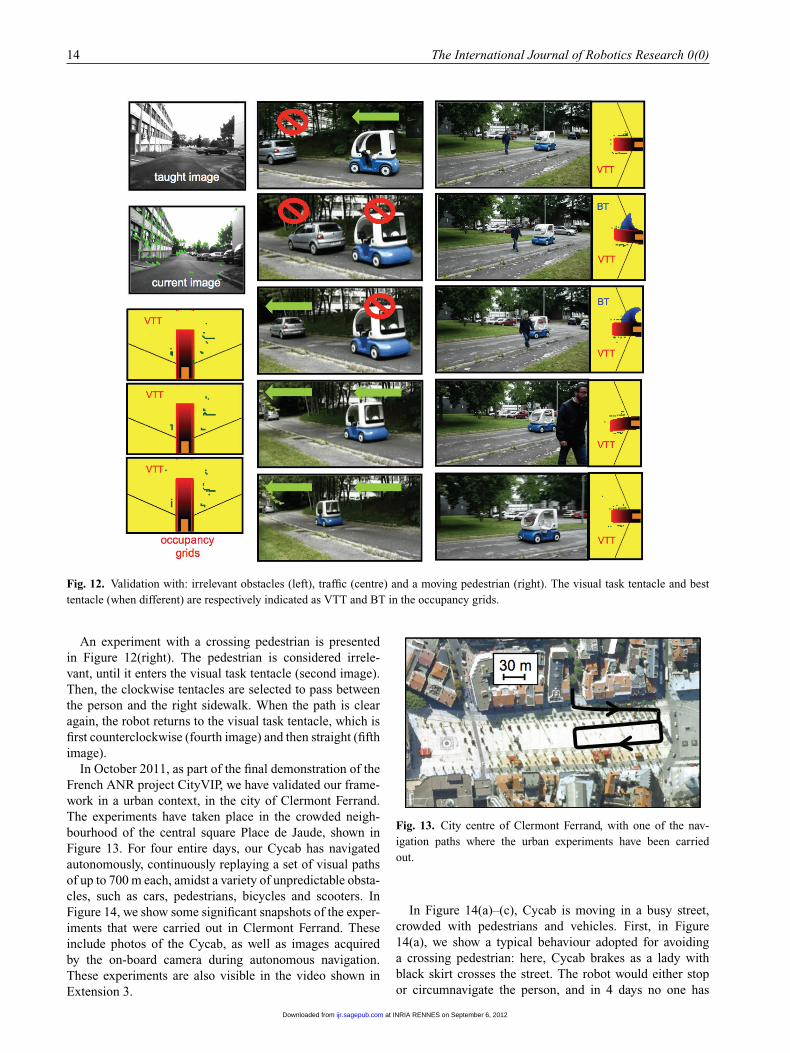
Again, by assessing the collision risk only along thevisual path, non-dangerous obstacles (e.g. walls or carsparked on the sides) are not taken into account. This aspectis clear from Figure 12(left), where a stage of the naviga-tion experiment on path E is illustrated. From top to bottom,we show the next key image in the database Id , the currentimage I and three consecutive occupancy grids processedat that point of the experiment. As the snapshots illustrate,the cars parked on the right (which were not present duringteaching) do not belong to any of the visual task tentacleclassification areas. Hence, they are considered irrelevant,and do not deviate the robot from the path.

Another nice behaviour is shown in Figure 12(centre): ifa stationary car is unavoidable, the robot decelerates andstops with (20), but, as soon as the car departs, the robotgradually accelerates (again with (20)), to resume naviga-tion. In fact, as we mentioned in Section 4, when the besttentacle is clear up to distance δs, a high velocity can beapplied: v = vs, independently of the value of H . In thefuture, this feature of our approach could even be utilizedfor vehicle following.




Fig. 12. Validation with: irrelevant obstacles (left), traffic (centre) and a moving pedestrian (right). The visual task tentacle and besttentacle (when different) are respectively indicated as VTT and BT in the occupancy grids.

An experiment with a crossing pedestrian is presentedin Figure 12(right). The pedestrian is considered irrele-vant, until it enters the visual task tentacle (second image).Then, the clockwise tentacles are selected to pass betweenthe person and the right sidewalk. When the path is clearagain, the robot returns to the visual task tentacle, which isfirst counterclockwise (fourth image) and then straight (fifthimage).

In October 2011, as part of the final demonstration of theFrench ANR project CityVIP, we have validated our frame-work in a urban context, in the city of Clermont Ferrand.The experiments have taken place in the crowded neigh-bourhood of the central square Place de Jaude, shown inFigure 13. For four entire days, our Cycab has navigatedautonomously, continuously replaying a set of visual pathsof up to 700 m each, amidst a variety of unpredictable obsta-cles, such as cars, pedestrians, bicycles and scooters. InFigure 14, we show some significant snapshots of the exper-iments that were carried out in Clermont Ferrand. Theseinclude photos of the Cycab, as well as images acquiredby the on-board camera during autonomous navigation.These experiments are also visible in the video shown inExtension 3.

Fig. 13. City centre of Clermont Ferrand, with one of the nav-igation paths where the urban experiments have been carriedout.

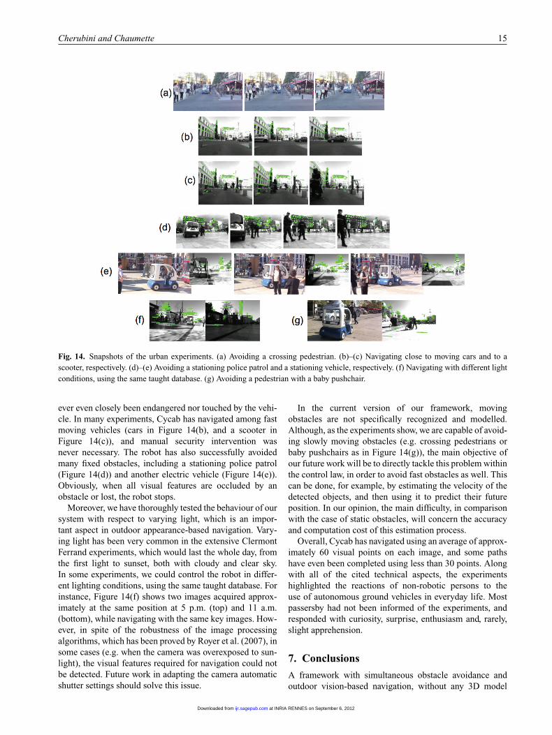
In Figure 14(a)–(c), Cycab is moving in a busy street,crowded with pedestrians and vehicles. First, in Figure14(a), we show a typical behaviour adopted for avoidinga crossing pedestrian: here, Cycab brakes as a lady withblack skirt crosses the street. The robot would either stopor circumnavigate the person, and in 4 days no one has




Fig. 14. Snapshots of the urban experiments. (a) Avoiding a crossing pedestrian. (b)–(c) Navigating close to moving cars and to ascooter, respectively. (d)–(e) Avoiding a stationing police patrol and a stationing vehicle, respectively. (f) Navigating with different lightconditions, using the same taught database. (g) Avoiding a pedestrian with a baby pushchair.

ever even closely been endangered nor touched by the vehi-cle. In many experiments, Cycab has navigated among fastmoving vehicles (cars in Figure 14(b), and a scooter inFigure 14(c)), and manual security intervention wasnever necessary. The robot has also successfully avoidedmany fixed obstacles, including a stationing police patrol(Figure 14(d)) and another electric vehicle (Figure 14(e)).Obviously, when all visual features are occluded by anobstacle or lost, the robot stops.

Moreover, we have thoroughly tested the behaviour of oursystem with respect to varying light, which is an impor-tant aspect in outdoor appearance-based navigation. Vary-ing light has been very common in the extensive ClermontFerrand experiments, which would last the whole day, fromthe first light to sunset, both with cloudy and clear sky.In some experiments, we could control the robot in differ-ent lighting conditions, using the same taught database. Forinstance, Figure 14(f) shows two images acquired approx-imately at the same position at 5 p.m. (top) and 11 a.m.(bottom), while navigating with the same key images. How-ever, in spite of the robustness of the image processingalgorithms, which has been proved by Royer et al. (2007), insome cases (e.g. when the camera was overexposed to sun-light), the visual features required for navigation could notbe detected. Future work in adapting the camera automaticshutter settings should solve this issue.

In the current version of our framework, movingobstacles are not specifically recognized and modelled.Although, as the experiments show, we are capable of avoid-ing slowly moving obstacles (e.g. crossing pedestrians orbaby pushchairs as in Figure 14(g)), the main objective ofour future work will be to directly tackle this problem withinthe control law, in order to avoid fast obstacles as well. Thiscan be done, for example, by estimating the velocity of thedetected objects, and then using it to predict their futureposition. In our opinion, the main difficulty, in comparisonwith the case of static obstacles, will concern the accuracyand computation cost of this estimation process.

Overall, Cycab has navigated using an average of approx-imately 60 visual points on each image, and some pathshave even been completed using less than 30 points. Alongwith all of the cited technical aspects, the experimentshighlighted the reactions of non-robotic persons to theuse of autonomous ground vehicles in everyday life. Mostpassersby had not been informed of the experiments, andresponded with curiosity, surprise, enthusiasm and, rarely,slight apprehension.

7. Conclusions

A framework with simultaneous obstacle avoidance andoutdoor vision-based navigation, without any 3D model




or path planning has been presented. It merges a novel,reactive, tentacle-based technique with visual servoing, toguarantee path following, obstacle bypassing, and colli-sion avoidance by deceleration. Since our method is purelysensor-based and pose-independent, it is perfectly suited forvisual navigation. Extensive outdoor experiments, even inurban environments, show that it can be applied in realisticand challenging situations including moving obstacles (e.g.cars and pedestrians). To the best of the authors’ knowledge,this is the first time that outdoor visual navigation withobstacle avoidance has been carried out in urban environ-ments at approximately 1 m s−1 on over 500 m, using nei-ther GPS nor maps. In the near future, we plan to explicitlytake into account the velocity of moving obstacles withinour controller, in order to avoid fast obstacles, which arecurrently hard to deal with. Perspective work also includesautomatic prevention of the visual occlusions provoked bythe obstacles.

Notes

1. See http://www.irisa.fr/lagadic/demo/demo-cycab-vis-navigation/vis-navigation.

2. Without loss of generality, we consider that intervals aredefined even when the first endpoint is greater than the second,e.g. [κn, κnn) should be read (κnn, κn] if κn > κnn.

3. At the first iteration, we set κpb = κn.4. See http://www.cyberbotics.com.

Funding

This work has been supported by ANR (French National Agency)CityVIP project (grant number ANR-07 TSFA-013-01).

References

Allibert G, Courtial E and Touré Y (2008) Real-time visualpredictive controller for image-based trajectory tracking of amobile robot. In International Federation of Automatic ControlWorld Congress, Seoul, Korea.

Becerra HM, Courbon J, Mezouar Y and Sagüés C (2010)Wheeled mobile robots navigation from a visual memory usingwide field of view cameras. IEEE/RSJ International Confer-ence on Intelligent Robots and Systems, Taipei, Taiwan.

Becerra HM, López-Nicolás G and Sagüés C (2011) A sliding-mode-control law for mobile robots based on epipolar visualservoing from three views. IEEE Transactions on Robotics 27:175–183.

Bonin-Font F, Ortiz A and Oliver G (2008) Visual navigationfor mobile robots: a survey. Journal of Intelligent and RoboticSystems 53: 263–296.

Bonnafous D, Lacroix S and Siméon T (2001) Motion genera-tion for a rover on rough terrains. In IEEE/RSJ InternationalConference on Intelligent Robots and Systems, Maui, HI.

Booij O, Terwijn B, Zivkovic Z and Kröse B (2007) Naviga-tion using an appearance based topological map. In IEEEInternational Conference on Robotics and Automation, Rome,Italy.

Broggi A, Bombini L, Cattani S, Cerri P and Fedriga RI(2010) Sensing requirements for a 13000 km intercontinen-tal autonomous drive. In IEEE Intelligent Vehicles Symposium,San Diego, CA.

Buehler M, Lagnemma K and Singh S (eds) (2008) Special Issueon the 2007 DARPA Urban Challenge, Parts I–III. Journal ofField Robotics 25(8–10): 423–860.

Chaumette F and Hutchinson S (2006) Visual servo control, PartI: Basic approaches. IEEE Robotics and Automation Magazine13(4): 82–90.

Chaumette F and Hutchinson S (2007) Visual servo control,Part II: Advanced approaches. IEEE Robotics and AutomationMagazine 14(1): 109–118.

Cherubini A and Chaumette F (2011) Visual navigation withobstacle avoidance. In IEEE/RSJ International Conference onIntelligent Robots and Systems, San Francisco, CA.

Cherubini A, Colafrancesco M, Oriolo G, Freda L and ChaumetteF (2009) Comparing appearance-based controllers for nonholo-nomic navigation from a visual memory. In ICRA Workshopon safe navigation in open and dynamic environments, Kobe,Japan.

Cherubini A, Spindler F and Chaumette F (2012) A new tentacles-based technique for avoiding obstacles during visual navi-gation. In IEEE International Conference on Robotics andAutomation, St. Paul, MN.

Courbon J, Mezouar Y and Martinet P (2009) Autonomous navi-gation of vehicles from a visual memory using a generic cam-era model. IEEE Transactions on Intelligent TransportationSystems 10: 392–402.

Davison AJ, Reid ID, Molton ND and Stasse O (2007)MonoSLAM: real-time single camera SLAM. IEEE Trans-actions on Pattern Analysis and Machine Intelligence 29:1052–1067.

De Luca A and Oriolo G (1994) Local incremental planning fornonholonomic mobile robots. In IEEE International Confer-ence on Robotics and Automation, San Diego, CA.

De Luca A, Oriolo G and Robuffo Giordano P (2008) Featuredepth observation for image-based visual servoing: theory andexperiments. The International Journal of Robotics Research27: 1093–1116.

Diosi A, Segvic S, Remazeilles A and Chaumette F (2011) Experi-mental evaluation of autonomous driving based on visual mem-ory and image based visual servoing. IEEE Transactions onIntelligent Transportation Systems 12: 870–883.

Durand Petiteville A, Courdesses M and Cadenat V (2010) A newpredictor/corrector pair to estimate the visual features depthduring a vision-based navigation task in an unknown environ-ment. In International Conference on Informatics in Control,Automation and Robotics, Rome, Italy.

Elfes A (1989) Using occupancy grids for mobile robot perceptionand navigation. Computer 22(6): 46–57.

Folio D and Cadenat V (2006) A redundancy-based scheme to per-form safe vision-based tasks amidst obstacles. In IEEE Inter-national Conference on Robotics and Biomimetics, Kunming,China.

Fontanelli D, Danesi A, Belo FAW, Salaris P and Bicchi A (2009)Visual servoing in the large. The International Journal ofRobotics Research 28: 802–814.

Goedemé T, Nuttin M, Tuytelaars T and Van Gool L (2007) Omni-directional vision based topological navigation. InternationalJournal of Computer Vision 74: 219–236.




Guerrero JJ, Murillo AC and Sagüés C (2008) Localization andMatching using the planar trifocal tensor with bearing-onlydata. IEEE Transactions on Robotics 24: 494–501.

Harris C and Stephens M (1988) A combined corner and edgedetector. In 4th Alvey Vision Conference.

Kato T, Ninomiya Y and Masaki I (2002) An obstacle detec-tion method by fusion of radar and motion stereo. IEEETransactions on Intelligent Transportation Systems 3: 182–188.

Khatib O (1985) Real-time obstacle avoidance for manipula-tors and mobile robots. In IEEE International Conference onRobotics and Automation, Durham, UK.

Lamiraux F, Bonnafous D and Lefebvre O (2004) Reactive pathdeformation for nonholonomic mobile robots. IEEE Transac-tions on Robotics 20: 967–977.

Lapierre L, Zapata R and Lepinay P (2007) Simultaneous pathfollowing and obstacle avoidance control of a unicycle-typerobot. In IEEE International Conference on Robotics andAutomation, Rome, Italy.

Latombe JC (1991) Robot Motion Planning. Dordrecht: KluwerAcademic.

Lee T-S, Eoh G-H, Kim J and Lee B-H (2010) Mobile robot nav-igation with reactive free space estimation. In IEEE/RSJ Inter-national Conference on Intelligent Robots and Systems, Taipei,Taiwan.

López-Nicolás G, Gans NR, Bhattacharya S, Sagüés C, GuerreroJJ and Hutchinson S (2010) An optimal homography-basedcontrol scheme for mobile robots with nonholonomic and field-of-view constraints. IEEE Transactions on Systems, Man, andCybernetics, Part B 40: 1115–1127.

López-Nicolás G and Sagüés C (2011) Vision-based exponen-tial stabilization of mobile robots. Autonomous Robots 30:293–306.

Lowe DG (2004) Distinctive image features from scale-invariantkeypoints. International Journal of Computer Vision 60:91–110.

Mariottini GL, Oriolo G and Prattichizzo D (2007) Image-basedvisual servoing for nonholonomic mobile robots using epipolargeometry. IEEE Transactions on Robotics 23: 87–100.

Minguez J, Lamiraux F and Laumond JP (2008) Motion planningand obstacle avoidance. In Siciliano B and Khatib O (eds.),Springer Handbook of Robotics. Berlin: Springer, pp. 827–852.

Nunes U, Laugier C and Trivedi M (2009) Introducing perception,planning, and navigation for intelligent vehicles. IEEE Trans-actions on Intelligent Transportation Systems 10: 375–379.

Ohya A, Kosaka A and Kak A (1998) Vision-based navigation bya mobile robot with obstacle avoidance using a single-cameravision and ultrasonic sensing. IEEE Transactions on Roboticsand Automation 14: 969–978.

Quinlan S and Khatib O (1993) Elastic bands: connecting pathplanning and control. In IEEE International Conference onRobotics and Automation, Atlanta, GA.

Royer E, Lhuillier M, Dhome M and Lavest J-M (2007) Monoc-ular vision for mobile robot localization and autonomous navi-gation. International Journal of Computer Vision 74: 237–260.

Scaramuzza D and Siegwart R (2008) Appearance-guided monoc-ular omnidirectional visual odometry for outdoor ground vehi-cles. IEEE Transactions on Robotics 24: 1015–1026.

Sciavicco L and Siciliano B (2000) Modeling and Control ofRobot Manipulators. New York: Springer.

Šegvic S, Remazeilles A, Diosi A and Chaumette F (2008) A map-ping and localization framework for scalable appearance-basednavigation. Computer Vision and Image Understanding 113:172–187.

Shi J and Tomasi C (1994) Good features to track. In IEEE Con-ference on Computer Vision and Pattern Recognition, Seattle,WA.

Tahri O and Chaumette F (2005) Point-based and region-basedimage moments for visual servoing of planar objects. IEEETransactions on Robotics 21: 1116–1127.

Von Hundelshausen F, Himmelsbach M, Hecker F, Mueller A andWuensche H-J (2008) Driving with tentacles-Integral struc-tures of sensing and motion. Journal of Field Robotics 25:640–673.

Wada T, Doi S and Hiraoka S (2009) A deceleration con-trol method of automobile for collision avoidance based ondriver’s perceptual risk. In IEEE/RSJ International Conferenceon Intelligent Robots and Systems.

Yan Z, Xiaodong X, Xuejun P and Wei W (2003) Mobilerobot indoor navigation using laser range finder and monoc-ular vision. In IEEE International Conference on IntelligentSystems and Signal Processing, Faro, Portugal.

Zhang Y, Lin WC and Chin Y-KS (2008) Driving skill characteri-zation: a feasibility study. In IEEE International Conference onRobotics and Automation, Pasadena, CA.

Zhang AM and Kleeman L (2009) Robust appearance basedvisual route following for navigation in large-scale outdoorenvironments. The International Journal of Robotics Research28: 331–356.

Appendix: Index to Multimedia Extensions

The multimedia extension page is found athttp://www.ijrr.org

Table of Multimedia Extensions

Extension Type Description

1 Video Simulations of our navigation schemein six different scenarios. In this andthe following two videos, the segmentslinking the current and next key imagepoints are drawn in light green in thecurrent image. In the occupancy grid,the dangerous cell sets associated withthe visual task tentacle and to the besttentacle (when different) are respec-tively shown in red and blue, and twoblack segments indicate the scanneramplitude. Only cells that can activateH (i.e. cells at distance � < �s) havebeen drawn.

2 Video Experiments on our campus.3 Video Extensive validation in the city centre

of Clermont Ferrand.



Documents

The International Journal of Robotics Research ... · ... Visual servoing is a well-known method that ... and Courbon et al. (2009),