Embed Size (px)
Citation preview

The interplayof the cell membranewith the cytoskeleton
Dissertationzur Erlangung des akademischen Grades
Doctor rerum naturalium(Dr. rer. nat.)
vorgelegt
der Fakultät Mathematik und Naturwissenschaftender Technischen Universität Dresden
von
Dipl.-Phys. Jochen Albert Max Schneidergeboren am 21. August 1985 in Berlin
Max-Planck-Institut für Physik komplexer Systeme
Dresden, 2016

Eingereicht am: 19. Februar 2016Verteidigt am: 27. Juni 2016
1. Gutachter (1st referee): Prof. Dr. Frank Jülicher2. Gutachter (2nd referee): Prof. Dr. Marino Arroyo


Acknowledgments
This thesis is dedicated to my former physics school teacher FrankPozniak. He raised my fascination for physics, which finally mademe choose physics at university and continue research afterwards,leading to my PhD work. This choice shall emphasize the importantrole of teachers for the development of children and their interestsfor subjects, which is, unfortunately, more and more underestimatednowadays. Not underestimated but equally important for a successfulcompletion of a PhD project is, besides the intrinsic fascination forthe subject, the support from family and friends. I am very glad thatI could rely on so many people every day. Special thanks shall goto my mother and my grandfather. My mother taught me how tobe persistent and determined and my grandfather has always beena shining example for the nobility of academia.
From the scientific point of view I would like to thank, pri-marily, my supervisor Guillaume Salbreux who introduced me tobiophysical research and guided me with great patience, enthusiasmand expertise. I also highly appreciated the advices of Frank Jüli-cher, director of the Biophysical Division at the Max Planck Institutefor the Physics of Complex Systems. It helped me to put the oftentechnical and detailed work into a broader scientific perspective. Mo-reover, I would like to thank all my colleagues who created a veryopen-minded, cooperative working environment, which led to manyfruitful discussions.
Moreover, I would like to thank the Max Planck Society andThe Francis Crick Institute for providing exceptional working con-ditions, which facilitated a very creative and focused work.
V


Abstract
Past work has attributed a major role for the mechanics and shapeof a biological cell to the cell cortex, a viscoelastic polymer networkunder contractile tension, and as the outermost part of the cell cy-toskeleton located beneath the cell membrane. Its importance hasbeen shown, for instance, for the spatial separation of daughter cellsduring cell division, for certain modes of cell migration and for themorphology of tissues. Furthermore, it has been discussed more re-cently that the contractility of the cortex can cause the membrane,which is anchored to the cortex via linker proteins, to buckle intoout-of-plane microstructures, such as bulges, buds and tubes. Thisobservation has been proposed as a fast mechanism to buffer occur-ring membrane excess area and as a regulator of membrane tension.
In this thesis we study the mechanical effect of cell membranebuckling by treating the cell membrane as an anchored lipid bilayerwith a surface tension and a bending energy. In order to accountfor the anchoring we introduce two different approaches. In the firstapproach we anchor a membrane with imposed surface area along adiscrete square lattice and calculate the resulting equilibrium sha-pe of the membrane. We find that within each lattice element themembrane shape is close to an axisymmetric shape if anchors arelocated on the edges of the square. Based on this finding, in thesecond approach, we model the membrane as a collection of axisym-metric protrusions where each protrusion is anchored along its basalboundary. The buckling shapes are determined by the membraneexcess area, a hydrostatic pressure difference across the membraneand a local point force, accounting for cortex filaments pushing onthe membrane. The membrane tension is set by the imposed mem-
VII
VIII J. Schneider
brane area. We then use this description of an anchored membraneto propose a model for the global cell mechanics and geometry basedon the interplay of cell membrane and cortex. This model involvesa closed system of equations describing the balance of osmotic andhydrostatic pressure differences, the force balance at the cell surfaceand a membrane area elasticity due to membrane fluctuations. Withthe help of this model we predict that the membrane takes a buckledshape as a result of the contractility of the cortex. We obtain sha-pe diagrams for the occurrence of out-of-plane membrane structures,such as blebs, microvilli and tubular invaginations, depending on thecontractility, the linker density and the cell osmolarity. Furthermo-re, we investigate the role of membrane buckling for cytokinesis, thefinal stage of cell division where the cell separates into two daughtercells. We show how a buckling asymmetry between the two cell po-les of the dividing cell can trigger a flow of lipids across the cleavagefurrow. Moreover, we hypothesize that the membrane buckling couldcause an effective surface elasticity helping to stabilize cell division.

Zusammenfassung
In der Vergangenheit wurde gezeigt, dass der Zellkortex, ein visko-elastisches, kontraktiles Polymernetzwerk direkt unterhalb der Zell-membran, als Teil des Zellskeletts eine bedeutende Rolle für die Me-chanik und die Form von biologischen Zellen einnimmt. WichtigenEinfluss hat er bei der Separation von Tochterzellen während derZellteilung, bei bestimmten Arten der Zellfortbewegung und bei derFormgebung von Zellgeweben. Weiterhin wurde kürzlich gezeigt, wiedie Zellmembran, die mittels spezieller Proteine mit dem Kortex ver-ankert ist, als Folge der Kontraktilität im Kortex kleine Wölbungen,Knospen und Finger ausbilden kann. Diese Deformationen tretenauf, um Zusatzmembran aufzufangen und die Oberflächenspannungder Membran zu regulieren.
In dieser Arbeit untersuchen wir den mechanischen Effekt derbeschriebenen Deformationen, in dem wir die Zellmembran als eineverankerte Lipiddoppelschicht mit assozierter Oberflächenspannungund Krümmungsenergie beschreiben. Um ihrer Verankerung Rech-nung zu tragen, folgen wir zwei Ansätzen. In ersterem verankernwir eine Membran mit gegebener Oberfläche entlang eines diskre-ten, quadratischen Gitters und berechnen die resultierende Gleich-gewichtsform der Membran. Wir finden, dass die Membran innerhalbjedes Gitterquadrats fast rotationssymmetrische, lokale Wölbungenausbildet, wenn Ankerpunkte auf den Kanten des Gittersquadratsplatziert sind. Darauf aufbauend modellieren wir mit dem zweitenAnsatz die Membran als Zusammenschluss von rotationssymmetri-schen Ausstülpungen, wobei jede dieser entlang ihres unteren Randesverankert ist. Sie sind weiterhin durch die vorhandene Zusatzfläche,einen hydrostatischen Druckunterschied zwischen beiden Membran-
IX

X J. Schneider
seiten, sowie durch eine Punktkraft, hervorgerufen von kortikalen Fi-lamenten, bestimmt. Die zugehörige Oberflächenspannung der Mem-bran bestimmen wir durch die Fixierung der Membranfläche. Wirbenutzen diese Beschreibung für eine verankerte Membran, um einModell für die globalen geometrischen und mechanischen Eigenschaf-ten der Zelle, basierend auf der Wechselwirkung von Zellmembranund -cortex, aufzustellen. Dieses Modell beinhaltet ein geschlossenesGleichungssystem für das Gleichgewicht von osmotischer und hydro-statischer Druckdifferenz, dem Kräftegleichgewicht an der Zellober-fläche und der Oberflächenelastizität, ausgehend von Membranfluk-tuationen. Mit Hilfe dieses Modells können wir schlussfolgern, dassaufgrund der Kontrakilität des Zellkortex lokale Deformationen derMembran auftreten. Noch größere Deformationen, wie Blasen, Mi-krovilli oder röhrenförmige Einstülpungen können wir mittels Pha-sendiagrammen vorhersagen, die von der Kontraktilität im Kortex,der Dichte der Membranankerpunkte und der Zellosmolarität abhän-gen. Des Weiteren untersuchen wir die Rolle der beschriebenen Mem-branwölbungen während der Zytokinese, der letzten Phase der Zell-teilung, wo sich die Zelle in zwei Tochterzellen zerteilt. Wir zeigen,wie eine Asymmetrie dieser Deformationen zwischen den beiden nochverbunden Tochterzellen zu einem Lipidfluss entlang der Teilungs-furche führen kann. Darüber hinaus stellen wir die Hypothese auf,dass diese Deformationen zu einer effektiven Oberflchenelastizitätführen, die zur Stabilisierung der Zellteilung beitragen könnte.


CONTENTS
List of important symbols 17
1 Introduction 191.1 Internal organization of eukaryotic cells . . . . . . . 20
1.1.1 The cytoskeleton and its function . . . . . . . 211.1.2 The cell membrane . . . . . . . . . . . . . . . 24
1.2 Cell division . . . . . . . . . . . . . . . . . . . . . . . 261.3 Physics of lipid bilayer membranes . . . . . . . . . . 28
1.3.1 The energy of curved lipid bilayer membranes 281.3.2 Shape fluctuations . . . . . . . . . . . . . . . 311.3.3 Equilibrium shape equations . . . . . . . . . . 33
1.4 Scope of this thesis . . . . . . . . . . . . . . . . . . . 38
2 A membrane bound at discrete anchoring points 452.1 Membrane anchors arranged on a square lattice . . . 462.2 Solution of the shape equation . . . . . . . . . . . . . 492.3 Mechanical properties for constant surface area . . . 52
2.3.1 Membrane surface tension . . . . . . . . . . . 522.3.2 Anchoring forces . . . . . . . . . . . . . . . . 56
2.4 Equilibrium shapes for constant surface area . . . . . 562.4.1 The limit of zero pressure difference and
corner anchors only . . . . . . . . . . . . . . . 58
13

14 CONTENTS J. Schneider
3 A membrane as a collection of protrusions 613.1 Shape equations for axisymmetric membrane
protrusions . . . . . . . . . . . . . . . . . . . . . . . 623.2 Equilibrium shapes for constant surface area . . . . . 66
3.2.1 For zero pressure difference . . . . . . . . . . 663.2.2 For inflating pressure differences . . . . . . . 683.2.3 For compressing pressure differences . . . . . 693.2.4 For an additional point force at the protrusion
tip . . . . . . . . . . . . . . . . . . . . . . . . 713.3 Mechanical properties for constant surface area . . . 74
3.3.1 Membrane surface tension . . . . . . . . . . . 743.3.2 Lateral membrane tension . . . . . . . . . . . 763.3.3 Vertical protrusion force . . . . . . . . . . . . 79
3.4 Combining protrusions to a membrane . . . . . . . . 793.4.1 Flow equation for the lipid exchange between
protrusions . . . . . . . . . . . . . . . . . . . 813.5 Equilibrium area distribution between coupled
protrusions . . . . . . . . . . . . . . . . . . . . . . . 823.5.1 Without force perturbations . . . . . . . . . . 853.5.2 With point force perturbations . . . . . . . . 873.5.3 With partial point force perturbations . . . . 88
4 Applications to cell biophysics 914.1 The cell membrane as a collection of protrusions . . 924.2 Cell mechanics based on the membrane-cortex
interplay . . . . . . . . . . . . . . . . . . . . . . . . . 944.2.1 Closed description . . . . . . . . . . . . . . . 944.2.2 Self-consistent solution . . . . . . . . . . . . . 98
4.3 Membrane blebs and tubes . . . . . . . . . . . . . . 1034.3.1 Caused by cortical filaments and lipid flow . . 1034.3.2 Caused by the discrete membrane anchoring . 106

CONTENTS 15
4.4 Cell membrane mechanics during cytokinesis . . . . . 1124.4.1 Membrane buckling due to cell pole
contractions . . . . . . . . . . . . . . . . . . . 1124.4.2 Flow equation for lipid exchange across the
cleavage furrow . . . . . . . . . . . . . . . . . 1154.4.3 Membrane buckling as a contribution for cell
elasticity during cytokinesis . . . . . . . . . . 120
5 Conclusions and outlook 125
A Differential geometry of surfaces 133
B Variational principle and the shape equations 137B.1 Variation calculus . . . . . . . . . . . . . . . . . . . . 137B.2 Shape equations in Monge parameterization . . . . . 139B.3 Shape equations in arc length parameterization . . . 143
C Derivation of the anchored membrane sheet solution 153
D Numerical solution for protrusion shapes 167
E Membrane protrusions in analytical limits 181E.1 Weak-bending approximation . . . . . . . . . . . . . 181E.2 Zero-rigidity approximation . . . . . . . . . . . . . . 186E.3 Tube approximation . . . . . . . . . . . . . . . . . . 189
F Alternative lateral tension expression 193
G Self-consistent solution for the membrane-cortex layer 197
References 201
List of figures 219


LIST OF IMPORTANT SYMBOLS
Geometrical quantities
Λ contour length of a membrane protrusion
Ω membrane excess area
ψ tilt angle between contour line and z-axis
ξ mesh size of the anchoring lattice
A (cell) membrane area
A‖ projected area of a membrane sheet
C0 spontaneous curvature
h elevation of membrane in z-direction
H, K mean curvature, Gaussian curvature
L elongation of a membrane protrusion in z-direction
l protrusion diameter
R cell radius
S apparent cell surface area
V (cell) volume enclosed by the membrane
Mechanical quantities
F (mechanical) membrane energy
17

18 CONTENTS J. Schneider
∆p pressure difference across the membrane
γ, γ∗ membrane surface tension, γ∗ = γ + κ2C
20
γ‖ lateral membrane tension
κ, κG bending rigidity, Gaussian rigidity
T temperature
σ stress
f point force at the membrane protrusion tip
fa anchor force per linker protein
K elastic modulus
T active contractile tension in the cell cortex
Other physical quantities
Πext external osmotic pressure of a cell
kB Boltzmann constant, kB = 1.380658 · 10−23 J K−1 [1]
Nint number of solute molecules inside the cell
Nl number of lipids
Np number of protrusions on the cell surface
t time
Other mathematical symbols
δ(x) Dirac delta function
δij Kronecker symbol
∇‖ two-dimensional Nabla operator
ρ, ϕ, z cylindrical coordinates
4‖ two-dimensional Laplace operator
s,u arc length and normalized arc length, u = 2s/Λ
x, y, z cartesian coordinates

INTRODUCTION 1
Biological organisms are known as one of the most complex systems.Their metabolisms and reproduction mechanisms follow actively1
driven, highly dynamic processes. Nevertheless, the progress in expe-rimental techniques during the last century, and therewith the abilityto observe and measure these processes quantitatively, is increasin-gly triggering the demystification of this complexity. Biochemicalpathways were identified as blueprints for signaling and remodelingin biology. Lately, physical principles have gained more attentionas a second important framework. Known and extended conceptsof thermodynamics and statistical physics, of mechanics and hydro-dynamics are used to describe many different biological processesacross all length scales.
This work applies mechanical concepts on the cellular level,more precisely on the outermost part of most eukaryotic cells, thecell membrane coupled to the underlying cytoskeleton. In this intro-ductory chapter we first give an overview of the internal cell organi-zation with an emphasis on cell membrane and outer cytoskeleton.Afterwards, we present previously developed physical concepts forthe description of lipid bilayer membranes. Both the biological andthe physical introduction are then used to motivate this work, based
1 Here active means under consumption of externally provided energy, see alsosection 1.1.1.
19

20 Introduction J. Schneider
nucleus
smoothendoplasmatic reticulum
roughendoplasmatic reticulum
liposomes
microtubule
cortex
membrane
microvilli
caveolae
mitochondrion
centro-some
Golgi apparatus
cytosol
Figure 1.1 | Illustration of the internal cell organization.
on recent experimental and theoretical findings. Finally, we give anoutlook to the following chapters.
1.1 | Internal organization of eukaryotic cells
The knowledge of the principal internal organization of living orga-nisms grew during the last centuries in the same way as the opticalobservation methods developed. Initial observations with simple op-tical lenses gave only a poor insight compared to modern techniquessuch as, for instance, confocal microscopy [2–4] or electron micros-copy [5–7]. One of the first key discoveries was that every biologicalorganism consists of minimal, self-sustaining entities, so-called bio-logical cells [8]. Since that time the progressive collection of further

1.1 Internal organization of eukaryotic cells 21
information led to a well accepted picture of the principal internalorganization of cells [9]. Based on this, organisms can be divided intothree domains: archaea, bacteria and eukaryotes [10]. The first twoare often summarized as prokaryotes. In this work we will focus oneukaryotic cells, in particular on animal cells. An illustration of theirprincipal internal structure is shown in Figure 1.1.
An important difference between prokaryotes and eukaryotesis that eukaryotic cells contain a cell nucleus. It hosts the deoxyri-bonucleic acid (DNA), which stores the genetic information of theorganism, and belongs to the group of organelles inside the cell (seeFigure 1.1 for other organelles). Each organelle fulfills a certain taskin the metabolism of the cell. Besides organelles, two other importantcellular structures are the cytoskeleton and the membrane, discussedfurther in the following.
1.1.1 | The cytoskeleton and its function
The cytoskeleton consists of three main protein polymer structures,microtubules, intermediate filaments (not shown in Figure 1.1) andactin filaments [9]. Together with multiple other associated proteinsthey are crucial for the shape and the mechanical properties of a celland also take part in the regulation of the internal cell traffic.
For this work the most important cytoskeletal structure is thecell cortex, which is a thin layer of about 200 nm thickness, locatedright underneath the cell membrane [11]. It is predominantly built bythe protein monomer actin, which has a typical diameter of 5 nm [12].These monomers polymerize to double-stranded, helical filaments,which are bundled and cross-linked via cross-linker proteins to apolymeric meshwork with mesh sizes ranging from 20 nm to 250 nm

22 Introduction J. Schneider
[13, 14]2. Such a meshwork is illustrated in Figure 1.2.The actin meshwork is highly dynamic as it undergoes a con-
tinuous turnover. This is, on the one hand, due to actin monomersattaching and detaching from filaments with a characteristic turno-ver time in the range of seconds to tens of seconds [16, 17]. On theother hand, also cross-linker proteins can change their actin bindingpartners at timescales comparable to those of actin turnover [17–19].As a consequence of the turnover, the cell cortex is a viscoelastic me-dium, elastic because of the dense meshwork geometry on time scalesshorter than the turnover time, viscous on larger timescales due tothe dynamic rearrangements within the meshwork [16,20–22].
Besides the viscoelastic character, the cell cortex is also an ac-tive medium. It is actively driven by two-headed bundles of myosinmotor proteins, which exert local forces to the meshwork by consu-ming energy from ATP hydrolysis [23]. On average, this leads to anactive contractile tension inside the cell cortex T , which can varyfrom 10 pN/µm to 1000 pN/µm, not only depending on the cell typebut also on the cell state [16, 24]. The exact details of the relation-ship between this active tension and the local force generation in themeshwork is not yet fully understood. However, experiments suggesta simple saturation relation between the tension and the number ofactive myosin motors Nm [25, 26]:
T = T effm
(1 +N∗)Nm
Nm +N∗N∗→∞−→ T = T eff
m Nm. (1.1)
Here N∗ is the characteristic saturation number which leads to alinear relationship between myosin motors and tension as it goes toinfinity. The coefficient T eff
m can be seen as an effective contribution ofa single myosin motor to the overall tension. In an order of magnitude
2 Thermal fluctuations have only a small influence on actin filaments in the cellcortex as their persistence length is of the order of 15µm [15].

1.1 Internal organization of eukaryotic cells 23
cortex
membrane
linkerlipid
cross-linker
actin filament
myosin motor
Figure 1.2 | Illustration of the cell membrane with the underlying cell cortex. Thearrows with the symbol τ indicate the turnover of actin monomers and(cross-)linker proteins (see text).
estimate it can be expressed as T effm ' fmflmf/Snmf, where nmf is the
number of myosin motors bundling to one motor filament, fmf theforce exerted by one such filament, lmf its length and S the apparentcell surface area, spanned by the cell cortex [27].
The cell cortex is also called actomyosin cortex because ofits multifaceted and dynamic properties dictated by actin and myo-sin. Due to these properties it is, to a large extent, the determiningcellular structure for the global mechanics and morphology of thecell [16, 28]. A prominent example is the cell rounding at the begin-ning of the final phase of cell division, caused by enhanced myosinactivity and thus enhanced contractile tension in the cortex [29–31].Other examples can be found in migrating cells where the interplayof tension and cortex remodeling can trigger the motility [32, 33],in early embryonal development where the actomyosin flow leads toleft-right symmetry breaking [34], or in multicellular systems whe-re the tension maintains the principal tissue structure and guidesmorphogenesis [35–38].
24 Introduction J. Schneider
1.1.2 | The cell membrane
The cell membrane is the outermost structure of eukaryotic cells. Itconsists of amphiphilic lipids with hydrophilic heads and hydrophobictails, which assemble to a bilayer with an inner and an outer leaftlet,where the hydrophobic tails face each other (see Figure 1.2). Thetypical thickness of the bilayer is of the order of 10 nm to whichthe hydrophilic head contributes with a radius of approximately0.5 nm [9]. Besides lipids itself the bilayer is enriched by differenttypes of membrane proteins. Those which are permanently embed-ded in the membrane are called integral membrane proteins, thosewhich only attach occasionally from the outside peripheral mem-brane proteins [39]. Both types play an important role for signaland nutrient transduction across the membrane and act as adhesionsites for other proteins inside and outside the membrane [9]3. Spe-cial channel proteins establish gateways for small particles, such asions [41]. Curvature inducing proteins, such as clathrin or caveolin,trigger cytosis, the intracellular transport of material via small li-pid vesicles called endosomes [42,43]. A particularly important classof proteins are the so-called linker proteins. They provide bindingsites for both actin filaments and integral membrane proteins and,thus, are responsible for the anchoring of the membrane to the cy-toskeleton. Common examples for these proteins are ezrin, radexinand moesin [44, 45]. Their mean distance lies between 0.2µm and1µm [46]. Equivalently to cross-linkers in the cell cortex also linkerproteins have characteristic turnover times. The turnover betweenlinker and cortex is of the order of less than a second, the turnoverbetween linker and membrane of the order of a few seconds [47].
Due to its many microscopic ingredients the cell membrane ishighly dynamic, driven by thermal and partly also active random
3 It is interesting to note that membrane proteins could make up to 30 % of allgenetically encoded proteins [40].

1.1 Internal organization of eukaryotic cells 25
processes. Its shape is undulated by thermal and actively stimula-ted fluctuations of different wavelengths [48–55]. Lipids can switchleaflets by spontaneous and induced flip-flop events. Most lipidsswitch on timescales of a day per lipid, however, some special typescan switch in only a few milliseconds [56–58]. Furthermore, lipidscan spin and, more importantly, diffuse laterally, in the same wayas membrane proteins. The diffusion constant of freely diffusing li-pids is of the order of 10µm2/s [59, 60]. The diffusion constant ofintegral membrane proteins is approximately one order below thatof lipids [61,62].
The diffusive character of the membrane motivated the deve-lopment of a relatively simple membrane picture, the mosaic mo-del [63]. Assuming an averaged shape without fluctuations, it re-gards the membrane as a locally flat, incompressible, two-dimensio-nal fluid, homogeneous in composition. However, recent observati-ons suggest that the actual membrane state is more complicated,of which two aspects are especially interesting for this work. First,the interaction between membrane and cell cortex via linker proteinscan divide the membrane into local compartments [13,64,65]. Corti-cal filaments act as fences and hinder the free diffusion between thedifferent compartments, a characteristic hop diffusion is observedinstead [59, 66]. Second, the membrane is often not completely flatattached to the cell cortex but exhibits small, persistent out-of-pla-ne microstructures, such as extracellular lipid assemblies, caveolae ormicrovilli [43,67–69]. Since the pure membrane reacts, indeed, inela-stic regarding lateral tensions4, these microstructures could act asmembrane buffers giving the membrane an effective extra expansi-bility [71–77]. Additionally, on time scales larger than a few minutesup to an hour, the modulation of endocytosis and exocytosis couldalso mediate the change of membrane area [78–82].
4 Experimentally lipid bilayers and cell membranes exhibited a maximal stretchof approximately 4 % close to lytic tensions of the order of 104 pN/µm [70].

26 Introduction J. Schneider
1.2 | Cell division
For the development of life in general and of multicellular organismsin particular it is crucial that cells replicate. Initially, different hy-potheses for this replication process were discussed, before, final-ly, it was observed that the replication is achieved by a periodicdivision of each mother cell into two equal daughter cells (see Fi-gure 1.3a,b) [83]5. Later, different cell phases prior the observabledivision were identified and summarized in the cell cycle [9]. It con-sists of the I-phase or interphase where the cell is growing and DNAis replicated, and the M-phase or mitotic phase where the actualdivision takes place.
The mitotic phase can be subdivided into mitosis and cytoki-nesis6. When the cell enters mitosis it rounds up by stiffening thecortex and increasing the tension in it [29–31,86,87]. At the same ti-me microtubules assemble into a spindle structure [88,89], for whichthe rounding acts as a stabilizer [86,90,91]. This spindle breaks thesymmetry of the cell and regulates the separation of DNA into twodaughter nuclei [92, 93]. At the end of this process the cell consistsof two cell poles (Figure 1.3a) and enters cytokinesis by ingressionof the cleavage furrow (Figure 1.3b) whose position is mainly deter-mined by the spindle [94–96]. Its ingression is caused by a contracti-le ring where myosin is further enhanced [97–101]. The contractionproceeds until the constriction becomes large enough to split the cellapart.
In a recent work Sedzinski et al. showed that during cytoki-nesis the position of the cleavage furrow can destabilize, sometimesaccompanied by oscillations of the cell pole volumes (Figure 1.3c,d)
5 In special cases also asymmetric divisions can occur [84] or the mother cell candivide into more than two daughter cells [85].
6 Besides mitosis meiosis is an alternative process, in which four daughter cellsdevelop, each with half the genetic information compared to the mother cell.

1.2 Cell division 27
a b c d
Figure 1.3 | Cell pole oscillations during cytokinesis. Here an L929 mousefibroblast cell is shown, which has already finished the internal preparation for celldivision, in a, e.g., two separate nuclei are visible. Under certain conditions (seetext), the spatial separation, accomplished by ingression of the cleavage furrow (b),can destabilize mechanically [26]. One pole of the cell contracts then, the otherexpands (c). Sometimes this leads to persistent oscillations with periodicexpansions and contractions on either side (d). Here one period lasts about 6min.b includes parameters for a theoretical modeling (see (1.2)). Image taken with abright field microscope, scale bar: 10µm [Images provided by Andrea Pereira,University College London].
and terminated by an aborted division [26]. A supporting theoreti-cal model describes the cell poles as overlapping spheres with poleradii R1 and R2 (see Figure 1.3), pole volumes V1 and V2, and theconserved total volume 2Vs. The shape evolution is described by thelinear dynamic ansatz
α
Vs
dV1
dt= − α
Vs
dV2
dt= −
[2T1
R1︸︷︷︸∆pLaplace
− 2T2
R2
]− K3D
Vs(V1 − V2), (1.2)
where α a friction coefficient. The right-hand side corresponds tothe total pressure difference between the cell-poles. It consists of anelastic term with the bulk compression modulus [102]
K3D := Vd∆p
dV
∣∣∣∣sym
, (1.3)
evaluated at the state where the two cell poles are symmetric and aterm ∆pLaplace, representing Laplace’s law [103, 104]. This, in turn,depends on the contractile tensions T1 and T2 inside the cortex of

28 Introduction J. Schneider
both poles. As is discussed in more detail in [26], these tensionsare coupled to the dynamics of actin, for which a second dynamicequation is proposed that takes into account the turnover of actinfilaments. Overall, the stability analysis of this model reveals that theobserved instability of cell division is triggered by three parameters:the tension in the symmetric case Ts, the turnover rate τ and thebulk elasticity K3D. It can be deduced that the following conditionmust be satisfied approximately in order to guarantee stable celldivision:
TsRsK3D
≈ 1. (1.4)
Here Rs is the radius of the two symmetric cell poles.
1.3 | Physics of lipid bilayer membranes
The physical modeling of cell membranes focuses mainly on twoaspects. One is the lateral organization of lipids and membrane pro-teins, e.g., by molecular dynamics simulations [105]. The second,which is relevant for this thesis, is the geometrical shape adopted bycell membranes. For simplicity, most of the past work has focusedhere on fluid membranes, ignoring the anchoring to an underlyingcell cortex. From now on, we will call these not anchored membraneslipid bilayer membranes or simply membranes.
1.3.1 | The energy of curved lipid bilayer membranes
The observation of non-spherical, e.g., biconcave, shapes of red bloodcells and lipid vesicles suggested that the shape of lipid bilayer mem-branes, in contrast to soap bubbles, is not only determined by sur-face tension [106–109]. In principle, these shapes can be describedby taking into account an additional bending rigidity, giving rise to a

1.3 Physics of lipid bilayer membranes 29
curvature energy [106, 110, 111]. Experimental measurements foundthat this rigidity is of the order of 20 kBT [112]. Several curvatureenergy expressions have been proposed, accounting for different li-pid bilayer properties such as slow flip-flop of lipids between leaflets(see section 1.1.2) [113, 114]. However, often it is sufficient to treatthe membrane as a single rigid layer. Especially for cell membranes,which consist of a lipid mixture, this is a good approximation, asthey usually contain components which can switch leaflets relativelyfast [57, 58]. Then the bilayer character is negligible. The curvatureenergy of such a simplified membrane is written in terms of the meancurvature H = (C1 +C2)/2 and the Gaussian curvature K = C1C2,where C1 and C2 are the principal curvatures of the surface (fordetails see appendix A). Together, H and K uniquely define thecurvature at each point of the membrane and the expression for theenergy is given by integrating the curvature over the entire membra-ne surface area A [110]:
FC =
∫dA[κ
2(2H − C0)2 + κGK
]. (1.5)
Here the bending rigidity κ, the Gaussian rigidity κG and the sponta-neous curvature C0 are intrinsic material properties of the membra-ne. The latter accounts for an asymmetry in the bilayer composition,e.g., different types of lipids in the inner and outer leaflet or a largernumber of proteins embedded in one of them. The model in (1.5) hasbeen the basis to study and verify many different membrane shapesof, for instance, vesicles [106,107,109,115], membrane tubes [116,117]and invaginations [118,119].
We use (1.5) in this work with some modifications and simpli-fications. First, we focus on closed surfaces. Then the Gauss-Bonnettheorem states that the integral over the Gaussian curvature is to-pologically invariant [120]. That is, if the membrane is not changing

30 Introduction J. Schneider
its topology this term gives only a constant contribution to the ener-gy. Second, throughout this work we assume that the compositionof the membrane is homogeneous. Then the parameters κ and C0
are constants and can be excluded from integration7. Furthermo-re, we add three further terms to (1.5) which introduce a couplingbetween physical and geometrical quantities: the coupling betweenthe surface tension γ and the surface area A of the membrane; thecoupling between the pressure difference ∆p := pint − pext accrossthe membrane and the volume V enclosed by the membrane; andthe coupling of a point force f perpendicular to the membrane andthe elongation L of the membrane at the position of the point force.Then the energy reads as8
F =κ
2
∮dA(2H − C0)2 + γA−∆pV − fL. (1.6)
For each of the introduced couplings two ensembles are distinguis-hable. Either the physical parameter is fixed and the geometricalquantity adjusts accordingly or the geometrical quantity is conser-ved and the related physical parameter acts as a Lagrange multiplier,ensuring the conservation of the associated geometrical parameter.One example is the often assumed conservation of membrane areaA. This gives an additional condition, which determines the surfacetension γ.
7 Reported gel-like membrane inhomogeneities, called lipid rafts, would modulatethe bending rigidity locally but seem to be relatively small in cells [121,122].
8 Note that in general the surface tension γ is not spatially invariant. However,as we assume here a homogeneous membrane composition γ adopts a constantvalue in the entire membrane.

1.3 Physics of lipid bilayer membranes 31
1.3.2 | Shape fluctuations
Since the bending rigidity of lipid bilayer membranes is roughly ofthe order of the characteristic thermal energy kBT its shape is un-dulated by thermal fluctuations [48,123]. A relatively simple mathe-matical description of these undulations can be derived by applyingthe energy (1.6) to an in average flat membrane assuming zero pres-sure difference, zero point forces and expanding the mean curvatureup to linear order9 [48]. This approach has been extended for otherenergy expressions [124–126] and for spherical and more complica-ted average shapes [127–129]. Also the effects of pressure [130], activefluctuations driven by cytoskeletal motor proteins [54, 131, 132] andthe effect of anchoring points to the cytoskeleton [133,134] have beendiscussed recently.
The thermally fluctuating membrane has a persistence lengthof [135,136]
ξp = lmic e4π3
κbkBT , (1.7)
where lmic is a microscopic length, e.g., the thickness of the mem-brane (see Figure 1.2). With a rigidity κb = 20 kBT the persistencelength becomes ξp ∼ 1034 µm and is thus many orders of magnitudelarger than the typical circumference of a cell, πR ∼ 10µm. The-refore, the membrane shape is determined by a persistent, averageequilibrium shape (see section 1.3.3), around which the membrane isfluctuating with small undulations [137].
For the average equilibrium shape effective parameters can beintroduced, in case of the energy (1.6) an effective bending stiffness,an effective surface tension and a projected area. These parametersarise from their bare counterparts, associated to the total membrane[132, 135, 136, 138, 139]10. In general, the relation between effective
9 See explanation on the weak-bending approximation in section 1.3.3.10The effective parameters are also called renormalized parameters.

32 Introduction J. Schneider
Figure 1.4 | Schematic of a fluctuatingmembrane. The dark gray dashed lineindicates the average equilibrium shapeof the membrane with an effective areaA, an effective surface tension γ and aneffective bending rigidity κ. The lightgray solid line marks a snapshot of thedynamic, thermal undulations around theequilibrium shape with the associatedbare quantities.
and bare quantities can be stated as
A = A(Ab,κb, γb), κ = κ(Ab,κb, γb), γ = γ(Ab,κb, γb), (1.8)
where the subscript b indicates the bare values and the not subs-cripted quantities shall be understood as effective quantities fromnow on. An illustration of the relation between bare and effectivequantities is provided in Figure 1.4. Physically the bare quantitiesare related to subcellular properties, e.g., the total area is appro-ximately proportional to the lipid number, Ab ∼ Nl. The effectivequantities, on the other hand, relate to cellular properties. Mostanalytical derived expressions for (1.8) studied flat membranes, onlyrecently curved geometries have been considered [130].
In this work we assume for the surface tension and the bendingrigidity that
κ ' κb, γ ' γb. (1.9)
Furthermore, we use an approximate relation between Ab and A,derived for flat membranes [138]:
Ab −AA
' kBT8πκ
log
[κq2
max + γ
κq2min + γ
]. (1.10)
Here qmin := π/lmem and qmax := π/lmic are the minimal and maxi-

1.3 Physics of lipid bilayer membranes 33
mal possible fluctuation modes of the membrane, respectively. Whe-reas the maximal mode is determined by the microscopic length oflipids, lmic ∼ 5 nm, the minimal mode is set by the characteristic sizeof the membrane. Equation (1.10) implies that in the limit of maxi-mal confinement of the membrane, when lmin ' lmax, the fluctuationsvanish and, thus, projected and total membrane area coincide, i.e.,A ' Ab.
1.3.3 | Equilibrium shape equations
The equilibrium shape of a lipid bilayer membrane, the average shapeof the fluctuating membrane, is defined as the shape which minimizesthe energy F and can be found mathematically by the variation ofthis energy [140]11. Here the energy (1.6) is given by the effectivequantities, introduced in section 1.3.2, and depends via the volume,the surface area and the curvature on the equilibrium shape and onlyon this. Hence, the energy minimum is uniquely determined by theequilibrium shape.
In order to find the equilibrium shape the variation of theenergy, denoted by δF , has to vanish. A general parameterizationindependent shape equation, which determines the equilibrium sha-pe, can be derived for the variation of (1.6) [141]. However, in manycases it is more convenient to start from a specific parameterization.This uniquely defines the position of the surface in the three-di-mensional space and depends only on two independent parametersu and v. The geometrical quantities of the energy (1.6) can thenbe expressed in terms of the chosen parameterization, as discussedin more detail in appendix A. The variation of the energy leads toa set of bulk and boundary terms, where the latter have to vanish
11The variation can also return unstable maximizing shapes, which, however, thesystem would leave eventually due to thermal fluctuations.

34 Introduction J. Schneider
identically, as discussed in appendix B, and the bulk terms give riseto a system of coupled partial differential equations, the so-calledEuler-Lagrange equations. These equations determine the equilibri-um shape upon integration constants which need to be specified byboundary conditions.
The choice of parameterization is arbitrary because any physi-cal quantity, in particular the energy, must be invariant under coor-dinate transformations [142]. Therefore, it is convenient to choosethe parameterization according to the principal geometrical featuresof the surfaces. In this work we use two different parameterizations,theMonge parameterization and the arc length parameterization. Forthe Monge parameterization, we set the point force f to zero.
Monge parameterization
In the Monge parameterization a height function h is used to describethe position of a surface with respect to a flat reference plane. Thisreference plane is parameterized by u and v which are chosen hereto coincide with the two cartesian coordinates x and y:
x = u, y = v, z = h(u, v) ≡ h(x, y). (1.11)
The one-dimensional case, where h is a function of x only, is illustra-ted in Figure 1.5a. The Monge parameterization is only well-definedif the slope of the surface remains finite in any point, i.e., the conditi-on arctan ‖∇‖h‖ < π/2 is satisfied. Here ∇‖ is the two-dimensionalnabla operator. In the context of the weak-bending approximation,often this condition is further confined by postulating ‖∇‖h‖ 1.This approximation is equivalent to very weak undulations of thesurface where h(x, y) is only changing slowly along the referenceplane. The surface can then be seen as a relatively flat rectangular

1.3 Physics of lipid bilayer membranes 35
a b
Figure 1.5 | Schematic of two special parameterizations for curves and surfaces. aMonge parameterization; b arc length parameterization.
sheet . As discussed in appendix B.2 in detail, the energy expressi-on for such a sheet can be linearized and the corresponding shapeequation deduces to
42‖h(x, y)− γ∗
κ4‖h(x, y) =
∆p
κ(1.12)
with the two-dimensional Laplace operator 4‖ and the renormalizedsurface tension
γ∗ := γ +κ
2C2
0 . (1.13)
The squared Laplace operator is called biharmonic operator. Theboundary terms, which also occur in the variation calculus, are ne-gligible for our later calculations. The square root of the ratio κ/γ∗
defines a characteristic bending length
λ =
√κ
γ∗. (1.14)
Since (1.12) is, in principle, solvable with analytical methods, theweak-bending approximation has been used extensively in the pastto study various questions regarding the shape of membranes [48,143–147].
36 Introduction J. Schneider
Arc length parameterization
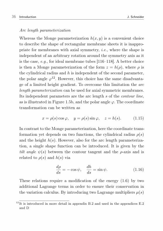
Whereas the Monge parameterization h(x, y) is a convenient choiceto describe the shape of rectangular membrane sheets it is inappro-priate for membranes with axial symmetry, i.e., where the shape isindependent of an arbitrary rotation around the symmetry axis as itis the case, e.g., for ideal membrane tubes [116–118]. A better choiceis then a Monge parameterization of the form z = h(ρ), where ρ isthe cylindrical radius and h is independent of the second parameter,the polar angle ϕ12. However, this choice has the same disadvanta-ge of a limited height gradient. To overcome this limitation the arclength parameterization can be used for axial symmetric membranes.Its independent parameters are the arc length s of the contour line,as is illustrated in Figure 1.5b, and the polar angle ϕ. The coordinatetransformation can be written as
x = ρ(s) cosϕ, y = ρ(s) sinϕ, z = h(s). (1.15)
In contrast to the Monge parameterization, here the coordinate trans-formation yet depends on two functions, the cylindrical radius ρ(s)
and the height h(s). However, also for the arc length parameteriza-tion, a single shape function can be introduced. It is given by thetilt angle ψ(s) between the contour tangent and the ρ-axis and isrelated to ρ(s) and h(s) via
dρ
ds= − cosψ,
dh
ds= sinψ. (1.16)
These relations require a modification of the energy (1.6) by twoadditional Lagrange terms in order to ensure their conservation inthe variation calculus. By introducing two Lagrange multipliers µ(s)
12 It is introduced in more detail in appendix B.2 and used in the appendices E.2and D

1.3 Physics of lipid bilayer membranes 37
and ν(s) the modified energy F∗ follows as
F∗ = F + µ
(dρ
ds+ cosψ
)+ ν
(dh
ds− sinψ
). (1.17)
The variation of (1.17) involves five functionals, namely δρ, δh, δψ,δµ and δν. A sixth degree of freedom for the equilibrium shape is theoverall contour length Λ of the surface. As a consequence, also theboundary positions of the contour line, s1 and s2, are not fixed andneed to be included into the variation [148]. Alternatively, the boun-daries can be chosen in such a way that the arc length ranges froms1 = 0 to s2 = Λ/2. Then the arc length can be normalized by Λ/2
and the new parameter u ranges from u1 = 0 to u2 = 1 and Λ entersthe energy by the coordinate transformation from s to u. The totalcontour length Λ is then an additional free parameter in the energy,while the integral boundaries remain constant. Overall, six coupled(differential) equations can be found from energy minimization, asdemonstrated in appendix B.3:
0 = −∆pΛρ2 cosψ − 8κ
Λρψ|uu + κΛ
sin 2ψ
ρ
+1
π
((4κψ|u − fΛ− 2Λν
)cosψ − 2Λµ|u sinψ
), (1.18)
0 = 2 γΛ + C20κΛ + 4C0κψ|u − 2∆pΛρ sinψ
− κΛsin2 ψ
ρ2+
4κ
Λψ2|u − 4µ|u, (1.19)
0 = ν|u, (1.20)
0 =Λ
2cosψ + ρ|u, (1.21)
0 = −Λ
2sinψ + h|u, (1.22)
0 = 2π
∫ 1
0du
[ρ
(2γ + C2
0κ−4κ
Λ2ψ2|u
)

38 Introduction J. Schneider
−2C0κ sinψ − f
πsinψ −∆pρ2 sinψ
+κsin2 ψ
ρ+ 2µ cosψ − 2ν sinψ
], (1.23)
where the notation |u := ∂∂u is used for simplicity. Equations (1.21)
and (1.22) ensure the consistency of the variation, as they coincidewith the imposed relations (1.16) between ρ and ψ and h and ψ,respectively. Equations (1.19) and (1.20) for µ and ν will serve asconstraint conditions for the two actual shape defining quantities,ψ(u) and Λ.
In addition to the shape equations, there are three boundaryterms
∂L∗
∂ψ|uδψ
∣∣∣∣10
=∂L∗
∂ρ|uδρ
∣∣∣∣10
=∂L∗
∂h|uδh
∣∣∣∣10
!= 0 (1.24)
with
∂L∗∂ψ|u
= −κρ(
sinψρ − ψ|s − C0
),
∂L∗∂ρ|u
= µ , ∂L∗∂h|u
= ν, (1.25)
and L∗ being the integrand of the energy F∗ (see (B.25) and (B.27)on page 144 and 144). With the help of imposed boundary conditionsthe boundary terms (1.24) can be evaluated and the shape equationscan be solved uniquely.
1.4 | Scope of this thesis
The first quantitative descriptions of cell membranes focused on tho-se aspects where the membrane can be treated as a lipid bilayer wi-thout interactions to the underlying cell cortex. Most remarkable arecontributions on membrane fluctuations, red blood cell shapes and

1.4 Scope of this thesis 39
the principal lateral organization of lipids and membrane proteins, asdiscussed in the previous sections. However, since novel microscopictechniques not only allow to observe the outer membrane but also thecortex beneath, more recent work started to explore the interactionbetween cell cortex and membrane. For instance, experiments deter-mined the critical force needed to detach the membrane from the cellcortex [149], resolved the compartmentalized microstructure of themembrane due to the underlying cortex meshwork [13, 64, 150] andstudied the biochemical pathways of binding [151]. Theoretical con-tributions proposed different concepts to account for the membrane-cortex interaction. Coarse-grained approaches introduced an energyexpression for the combined membrane-cortex layer [152,153] or as-sumed a continuos adhesion energy [70]. Others treated the inter-action by ligand-receptor binding kinetics [154] or by anchoring themembrane at spatially localized pinning sites [133, 155–158]. Theseconcepts have been used to describe hindered diffusion and its influ-ence on the formation of ordered lipid microdomains [153,159–162].Also the effect on membrane fluctuations has been discussed whereboth the anchoring itself and also the perturbation induced by activefluctuations inside the cortex are important [133,134,157,158]. Thelatter has also been identified as the driving mechanism for trans-versal propagating membrane waves [131,163].
Another large group of studies focused on mechanisms, trig-gered by membrane-cortex interactions, which cause the deforma-tion of the cell membrane into local, persistent out-of-plane struc-tures13. Blebs form when the membrane detaches locally from thecortex or the cortex ruptures locally [149, 164–166]. Microvilli areinduced by actin bundles pushing from the inside against the mem-brane [167]. Buds and caveolae are mediated by membrane prote-
13Here the term persistent is used to distinguish these structures from non-persi-stent fluctuations.

40 Introduction J. Schneider
Figure 1.6 | Local membrane deformations during cytokinesis. The images show aL929 mouse fibroblast cell during cytokinesis. The left image has been taken with aconfocal microscope, where the intensity is proportional to the membrane markerCAAX. The right image has been taken with an electron microscope (a single sliceof the cell). Both give evidence for an accumulation and ruffling of membrane onthe smaller cell pole, whereas on the other pole the membrane is rather smooth.[Images provided by Andrea Pereira (left) and Ortrud Wartlick (right), UniversityCollege London].
ins [119, 168–171]. Local contractions of the cell cortex can stimu-late the formation of unmediated collections of buds, bulges andtubes [155,172–177].
In this context recent experiments with mouse fibroblast cellsduring cytokinesis raised our attention. As discussed in section 1.2,under certain conditions their cleavage furrow position can destabi-lize, resulting in volume oscillations between the two daughter cellpoles [26]. Very recently, Andrea Pereira and Ortrud Wartlick fromEwa Paluch’s group14 have provided confocal images of the labeledcell membrane as well as electron microscopy images, both shown inFigure 1.6. Such images indicate that cell pole oscillations also affectthe shape of the cell membrane. On the side of the contracting po-le the membrane strongly accumulates into small buds, bulges andmicrovilli, on the expanding side it appears relatively flat.
The finding of these local membrane structures provokes the
14Medical research Council, Laboratory for Molecular Cell Biology, University Col-lege London, UK.

1.4 Scope of this thesis 41
Figure 1.7 | Illustration of membrane buckling induced by lateral compression.When the underlying substrate or cell cortex of the membrane, to which themembrane is attached, contracts or is compressed, the membrane can locallybuckle as studied in [155,175]. The buckling can lead to the formation of differentprotrusion types, such as buds and tubes [175].
following questions: How can the appearance of these structures,that are rather triggered by forces than by proteins, be understoodin a larger cellular context? That is, on the one hand, how exactlydoes the cortex mechanics influence the membrane? How do cortexcontractions induce membrane protrusions, what types, and how isthe membrane tension modified then? On the other hand, can themechanical state of the membrane, in turn, also affect global mecha-nical properties of the cell, which are assumed to be dictated, to alarge extent, by the cell cortex?
Partly, these questions have been addressed previously. Anoverall cell surface tension, consisting of contributions from both thecortex and the membrane, has been used to determine the mecha-nical equilibrium of the cell via Laplace’s law [154]. The magnitudeof the surface tension has been proposed to regulate the ability ofa cell to form extrusions, such as blebs and lamellipodia, used, e.g.,for cell migration [178, 179]. Three other studies are especially re-lated to the experimental observations for dividing cells, discussedabove (Figure 1.6): Staykova et al. have shown in vitro that a li-pid bilayer coupled to an underlying elastic substrate responds to

42 Introduction J. Schneider
a compression of the substrate with a local buckling, i.e., detach-ment of the membrane from the substrate (see illustration in Figu-re 1.7) [174,175]. This buckling is due to the fact that lipid bilayersare effectively incompressible and thus must compensate the late-ral compression by storing excess area in out-of-plane structures.As Staykova et al. quantified, these structures take the form of bul-ges and can eventually turn into tubular or spherical protrusions,upon a further compression of the substrate. This finding is remar-kable because it demonstrates that the formation of such localizedout-of-plane structures does not require the assistance of curvatureinducing molecules, as studied previously [180]. Instead a pure me-chanical stimulus is sufficient. The idea that forces can induce mem-brane buckling has also been discussed by Sens et al. to describe redblood cell shedding [73,155]. They apply the concept of force balan-ce to the anchoring points where the cell membrane is attached tothe underlying contractile cortex. Above a critical contractility thetightly attached membrane buckles, forms a bulge and may, even-tually, vesiculate. Finally, Lenz et al. showed that even in absenceof contractility an intrinsic curvature of cortex filaments can inducebuckling [177].
Although the mentioned investigations made important con-tributions for the addressed questions, a global cellular descriptionwhich combines cortex and membrane mechanics and, at the sametime, accounts for the formation of membrane microstructures is yetmissing. It is the main goal of this thesis to introduce such a descrip-tion. It shall be simple enough to give analytical insights but alsocapable to provide interesting physical implications, of which somewill be discussed here.
We will begin in chapter 2 with a relatively flat membrane,which is anchored at discrete points to an underlying square lattice,comparable to the previously suggested fence-like structure, induced

1.4 Scope of this thesis 43
membrane
linker
actin filament
Figure 1.8 | Illustration ofan anchored membranebuckled due to availableexcess area.
by the underlying filamentous cortex meshwork [59, 66]. We will in-troduce a physical description which allows to calculate analyticallythe out-of-plane membrane shape, depending on the given excessarea (compared to the projected square), a hydrostatic pressure dif-ference across the membrane and the anchoring configuration. Anillustration of such a model membrane is shown in Figure 1.8. Inchapter 3 we will then assume that the bulge-like structure, occur-ring in each of these square lattice elements, can roughly be treatedas an axisymmetric protrusion and will therewith propose a modelmembrane setup by a collection of protrusions. This model accountsfor more complicated protrusion geometries such as tubes and buds,for which we will study the stability. We will then assume that thismodel can be used, in good approximation, to describe a cell mem-brane anchored to the underlying cell cortex. Based on this, we willdescribe in chapter 4 the outer shell of the cell as a coupled layerof cortex and membrane, from which the membrane surface tensi-on and shape, the pressure difference between cell inside and outsideand the cell radius can be determined independently. We will use this

44 Introduction J. Schneider
description to study the formation of blebs and microvilli in cells,depending on the cortical tension and the external osmotic pressure.Moreover, we will discuss the experimental observations, shown inFigure 1.6, quantitatively. In the last chapter we will conclude ourfindings and will give a brief outlook of potential future interests.

A MEMBRANE BOUND
TO DISCRETE ANCHORING POINTS 2
Summary: As we have discussed in section 1.4, in some situationsthe cell membrane can be structured into different types of localprotrusions. The ability of forming them arises from available excessarea, which is distributed on a smaller cellular apparent surface area.Moreover, the membrane is also constrained by the underlying cellcortex as it is attached to it by linker proteins. This fact motivatesthe question how this attachment affects the exact structuring ofavailable excess area and if it can trigger particular local out-of-planeshapes.
In this chapter we approach this question by developing asimplified analytical membrane model where a membrane is tightlyanchored at discrete points, which are periodically arranged on aflat square lattice1. We study the resulting membrane structure, theforces exerted on the anchoring points and the surface tension withinthe membrane as a function of excess area, pressure difference andthe exact arrangement of anchoring points. Based on this, we findthat, as soon as anchors are not only placed at the corners of thesquare lattice but also along the edges, the preferential out-of-planeshape is given by membrane bulges with almost axial symmetry, one
1 A related description, based on a different modelling approach, has been sugge-sted previously in [156,181].
45

46 A membrane bound at discrete anchoring points J. Schneider
Figure 2.1 | Illustration of amembrane sheet. A is here the totalmembrane area, A‖ the areaprojected in the x-y -plane andpint − pext the pressure differenceacross the membrane.
bulge located in each of the lattice squares. If the anchors are locatedin the corners only and the pressure difference is zero, we find, besi-des the bulge-like pattern, a second ridge-like pattern, which exhibitslong-range folds.
2.1 | Membrane anchors arranged on a square lattice
Throughout this chapter we regard the lipid bilayer membrane asa thin, infinitely spread sheet with only weak shape undulations assketched in Figure 2.1. In this limit we can use the Monge paramete-rization in the weak-bending approximation to describe its elevationh as a function of x and y (see section 1.3.3). Furthermore, we treatthe membrane sheet in the constant effective area ensemble wherethe total number of lipids and, thus, the total area stored in fluctua-tions Ab is undetermined but the average area A is fixed. Since thesheet is infinitely extended along the axes, it is useful to normalize Aby the projected area A‖ underneath the membrane in order to havea finite area measure. The area conservation can then be written as
Ω :=A
A‖− 1
!= const. (2.1)
The quantity Ω is a measure for the excess area of the membranesheet in relation to its projected area. Condition (2.1) determines

2.1 Membrane anchors arranged on a square lattice 47
the surface tension γ, which acts as a Lagrange multiplier then.Additionally, a pressure difference ∆p = pext − pint > 0 is appliedacross the membrane, where pint is below the membrane and pextabove (see Figure 2.2b).
The exertion of a non-vanishing pressure difference ∆p on afree membrane sheet would lead to an accelerated shift of the sheettowards the lower pressures. Such a shift is suppressed when themembrane is fixed at discrete anchoring points. As then the mem-brane remains at rest, the force exerted by the pressure differencemust be compensated by a resistive force provided by these ancho-ring points. This is illustrated in Figure 2.2b where the anchoredmembrane is sketched in a side view. At the anchoring points (darkgray) an outward pointing force fout (blue), generated by a largerpressure pint compared to pext, is balanced by the inward force fin(red).
In principle, any spatial distribution of membrane anchoringpoints, holding the membrane in position, is conceivable. For simpli-city, we study the simplified case where anchoring points are arran-ged at equal height on a two-dimensional, quadratic, periodic latticewith mesh size ξ, shown in Figure 2.2a. Examples of different unitelements for this lattice are shown in Figure 2.2c. The unit elementsare symmetric with respect to the x and y direction and the anchorsare placed equidistantly along the edges. Their number is tunable bya parameter q. For q = 0 anchoring points are only located at eachcorner of the lattice. For q = 1 one additional intermediate anchor isplaced on each edge and for q = 2 two. We can formalize the positionof the anchors by the function
Gmn;s = δ(x− ξn− xs)δ(y − ξm− ys) (2.2)

48 A membrane bound at discrete anchoring points J. Schneider
Figure 2.2 | Membrane sheet bound to a square lattice of discrete anchoringpoints. In a a top view with indicated anchoring mesh (dashed lines) of mesh size ξis shown. b provides a side view of the membrane bound by anchors. c shows threedifferent examples of unit lattice elements. At each lattice corner one anchoringpoint is located. Additional anchors can be placed in between along the edges ofthe lattice. The value q defines the exact number of such intermediate anchors.
with the chosen coordinate representation
xs =
sq−1ξ 0 ≤ s ≤ q,
0 q < s ≤ 2q,(2.3)
ys =
0 0 ≤ s ≤ q,
s−qq−1ξ q < s ≤ 2q.
(2.4)
Here the indices n and m label the different lattice elements, bothrunning from −∞ to ∞, and s the individual anchors within oneunit element, running from 0 to 2q.
With the help of the function Gmn;s we can deduce the shapeequation for a membrane sheet constraint by periodically arrangedanchors. It is given by (1.12) on page 35 with additional terms arisingfrom the resistive force f (s)
a at the position of the anchors:
42‖h(x, y)− γ∗
κ4‖h(x, y) =
∆p
κ+
2q∑s=0
f(s)a
κ ξ2
∑n,m
Gmn;s. (2.5)

2.2 Solution of the shape equation 49
The introduced resistive forces are determined by ensuring that allanchoring points remain at the same height, independent of the choi-ce of ∆p. We discuss this in more detail in the following section.From symmetry arguments, identical anchors in the neighboring lat-tice elements must experience the same force. Only the forces withinone unit element can differ between the anchors. That is why theforces only carry the index s.
For convenience, we use dimensionless quantities from now on.We first introduce a normalized energy F := F/κ. Secondly, with themesh size ξ we can normalize the coordinates to x := x/ξ, y := y/ξ
and h := h/ξ. Furthermore, we then introduce a normalized pressuredifference ∆p, normalized anchor forces f (s)
a , normalized spontaneouscurvature C0 and normalized surface tension γ as follows:
∆p :=ξ3
κ∆p, f
(s)a :=
ξ
κf (s)a , C0 := ξ C0, γ :=
ξ2
κγ. (2.6)
Moreover, in Monge parameterization in weak-bending approxima-tion the excess area can be expressed as (see also Table B.1 on page150)
Ω ≡ 1
2
∫ 1
0dxdy∇‖h
2. (2.7)
2.2 | Solution of the shape equation
Using the weak-bending approximation has the advantage that theresulting shape equation (2.5) can be solved analytically. This canbe done by computing the fundamental solution hf of (2.5) and con-struct the solution h as the convolution of hf with a source termQ [182]:
h(x, y) = (Q ∗ hf)(x, y). (2.8)

50 A membrane bound at discrete anchoring points J. Schneider
As a source term we understand in this context the inhomogeneityof a differential equation. In our case it is given by the right-handside of (2.5).
The solution (2.8) uniquely describes the boundary value pro-blem with sources up to an arbitrary gauge function h0 which satis-fies the homogeneous problem[
4‖2 − γ∗4‖
]h0(x, y) = 0. (2.9)
Any such h0 can be added to the solution h without changing itsvalidity [183]. In particular, this includes a constant solution. Wemake use of this to gauge h(x, y) such that the anchoring points arealways located at z = 0.
In detail, the derivation of h, according to (2.8), is explainedin appendix C. Here we summarize a few key aspects. First of all,from the construction of the fundamental solution hf we concludethat the Fourier transform of (2.8) is given by2:
h(kx, ky) =Q(kx, ky)
k4
+ γ∗k2 . (2.10)
The hatted quantities are those in the Fourier k-space, where k isthe normalized wave number vector with the cartesian componentskx and ky. The sought profile h(x, y) can then be calculated by theinverse Fourier transformation of (2.10) if, beforehand, the Fouriertransform Q(kx, ky) can be computed. In case of our shape equati-on (2.5) this is relatively easy because the Fourier transformation ofthe source term reduces to the transformation of standard functions.The resulting function Q(kx, ky) contains δ-distributions only. Two
2 The definition of the Fourier transformation, used here, is given by (C.4) and(C.5) on page 154.

2.2 Solution of the shape equation 51
terms are proportional to the zeroth mode δ-distribution δ(kx)δ(ky).Each of them would lead to a divergence of the height profile, dueto the denominator of (2.10). The reason for this divergence lies inthe origin of these two terms. One of them corresponds to the pres-sure difference ∆p, the other to the resistive anchoring forces f (s)
a .If only one of both would be present, the membrane sheet would bedisplaced continuously until infinity. Thus, the divergence originatesfrom an unbalanced force exerted on the membrane. However, thiseffect is eliminated as we introduced the resistive forces such thatthey exactly balance the pressure difference and the membrane sheetis held in place.
The matching of the two zeroth mode terms leads to one de-fining condition for f (s)
a . In total 2q + 1 such conditions are neededto uniquely determine all anchoring forces within one unit element.The remaining 2q follow from the fact that the anchors are all keptat the same height. All 2q + 1 conditions can be summarized in amatrix equation, which determines all f (s)
a :
2q∑s=0
M lsf(s)a = N l, (2.11)
where M is a square matrix with the entries
M ls =
1 for l = 0,
Γγ∗(xl − xs, yl − ys)− Γγ∗(x0 − xs, y0 − ys)
otherwise,(2.12)
and N a vector with the entries
N l =
−∆p for l = 0,
0 otherwise.(2.13)

52 A membrane bound at discrete anchoring points J. Schneider
The used function Γα(x, y) is defined as
Γα(x, y) :=1
4π4
∑n,m≥1
cos (2πnx) cos (2πmy)
(n2 +m2)2 + α4π2 (n2 +m2)
+1
8π4
∑n≥1
cos (2πnx) + cos (2πny)
n4 + α4π2n2
.
(2.14)
Also the final height profile of the anchored membrane sheet can beexpressed by Γα:
h(x, y) =
2q∑s=0
f(s)a[Γγ∗(x− xs, y − ys)− Γγ∗(xs, ys)
]. (2.15)
2.3 | Mechanical properties for constant surface area
2.3.1 | Membrane surface tension
For a membrane sheet with fixed (normalized) surface tension γ∗
(2.15) together with (2.11) would be enough to describe it. However,since we want to study the shape for a fixed effective surface area wehave to adjust γ∗ accordingly. This is achieved by plugging h(x, y)
from (2.15) into the area relation (2.7) and solving it for γ∗. Ingeneral, this cannot be done with analytical methods. Instead itneeds to be solved numerically as we explain in appendix C. For thecorresponding solution γ∗ we find that
γ∗ = γ∗(Ω, ∆p). (2.16)
In fact, γ∗ is only a function of one independent parameter, definedby the ratio3
β =∆p
2
Ω. (2.17)
3 A plot of γ∗(β) is provided in Figure C.3 on page 165.

2.3 Mechanical properties for constant surface area 53
-40
-20
0
0 1 2
γ∗
Ω
q = 0
q = 2
q = 1, 3 0
200
400
0 300 600 900
γ∗
∆p
q = 0
q = 1
q = 2, 3
Figure 2.3 | Surface tension of an anchored membrane sheet. Plotted as afunction of the excess area with a constant pressure difference ∆p = 100 (left), asa function of the pressure difference with a constant excess area Ω = 0.1. Both isplotted for different anchor configurations as indicated.
This ratio shows that pressure and excess area have inverse effectson the surface tension. Increasing the pressure is qualitatively thesame as decreasing the excess area. The quantitative dependenciesare shown for four different anchor configurations in Figure 2.3. Inthe limit of a large pressure difference, with a constant finite excessarea, γ∗ increases linearly with ∆p. More precisely, we find that
γ∗ ∝ r∗√Ω
∆p for β →∞. (2.18)
Here r∗ is a numerical constant specified in Table 2.1. The limit oflarge pressure difference is equivalent to the limit of Ω→ 0. In bothcases β goes to infinity. Hence, the found approximation (2.18) alsodescribes the divergent behavior of γ∗ near Ω = 0. Qualitatively, thisdivergence can be understood in the following way: A finite pressuredifference will always tend to buckle the membrane sheet. This buck-ling can only be suppressed by putting the membrane under infinite

54 A membrane bound at discrete anchoring points J. Schneider
Table 2.1 | Numerical values corresponding to the asymptotic behavior ofγ∗(Ω,∆p). The constants correspond to the following relations:γ∗ ∝ γ∗0 + r∗0∆p/
√Ω (β → 0), γ∗ ∝ r∗∆p/
√Ω (β →∞) and γ∗(β0) = 0. The
constants are obtained analytically and their precision is determined by theexpansion order of the height profile h (see appendix C).
q β0 [105] γ∗0 r∗−2
0 r∗−2
0 0.264 −4π2 2π2 5.64
1 2.71 −51.8 124 22.1
2 2.78 −50.7 114 38.0
3 2.91 −52.0 112 45.1
positive tension. On the other hand, for ∆p→ 0 the surface tensionalways becomes negative, as it also does for increasing Ω, until it,eventually, reaches a minimal negative value γ∗0, provided in Table2.1. In principle, the occurrence of a negative surface tension canbe understood by the curvature caused by excess area. More excessarea is equivalent to more curvature and is energetically less favora-ble according to our energy ansatz. Hence, if possible, the membranewould exclude lipids in order to reduce its curvature and, thus, theenergy. This tendency gives rise to a negative surface tension wherethe lipids have to resist a squeezing. In fact, this mechanism canalso explain why the surface tension is always significantly lower forq > 0 compared to q = 0. At ∆p = 0 the enhanced constraining ofthe shape, due to more anchors, leads to a larger curvature of themembrane sheet. This leads, according to our previous arguments,to a lower surface tension. Secondly, more anchors damp the impactof the pressure difference on the membrane shape. That is why γ∗
also increases more slowly for q > 0. Both aspects can be concluded

2.3 Mechanical properties for constant surface area 55
-300-250-200-150-100-500
50f(s)
a
∑f(s)a
iii
q = 1
i ii
ii ∑f(s)a
i
ii
-300-250-200-150-100-500
50
0 1 2
Ω
iii
iii
q = 3
i ii iii ii
ii
iiiii
100 200 300 400
∆p
iii
iii
Figure 2.4 | Resistive forces at the membrane anchoring points. Plotted are twoexamples for the configurations q = 1 (top) and q = 3 (bottom). For varying area(left) a constant pressure difference ∆p = 100 is used and for varying pressuredifference (right) a constant area Ω = 0.5 is used. The inset schematics give anorientation for the position of the respective anchor. The dashed line indicates thetotal anchoring force, which has to be equal to −∆p.
from the energy F of one unit element of the membrane sheet, shownin Figure C.2b on page 162. At ∆p = 0, where F coincides with thecurvature energy FC, F is larger for q > 0 than for q = 0, indica-ting the larger curvature. And for ∆p > 0 it changes more slowly,indicating the effect of pressure on the shape is weaker.

56 A membrane bound at discrete anchoring points J. Schneider
2.3.2 | Anchoring forces
Having the surface tension γ∗ we can compute the force f (s)a via
(2.11). The result is shown for two example configurations at q = 1
and q = 3 as a function of Ω and ∆p in Figure 2.4. The two most im-portant observations are these: Firstly, although (2.11) implies that∑
s f(s)a = ∆p, each individual force f (s)
a does not converge necessari-ly to zero for ∆p→ 0. This is only the case if also Ω→ 0 (not shownin Figure 2.5). That is, also the curvature of the membrane sheet,due to the excess area, feedbacks to the anchoring points. This meansthat the anchors do not only prevent the membrane from detachmentdue to pressure difference but also from invagination. This finding isrelated to the second important observation, namely that f (s)
a cantake both values smaller and larger than zero. The case f (s)
a < 0
corresponds to a membrane pulling on the anchors, f (s)a > 0 to an
inward pushing. Thus, curvature and pressure difference affect thesign of the forces similarly as this of the surface tension. Increasing∆p at constant Ω leads, eventually, to a pulling force at all ancho-ring points (Figure 2.4 right). A larger excess area can reduce thispressure induced pulling at some anchoring points so that the forcedirection is inverted (see, e.g., Figure 2.4 left, anchor i). In general,the pressure difference seems to have a larger impact on the middle-most anchors, the curvature on those closer located to the corners ofthe lattice. To check the consistency of these observations, we alsoplotted in Figure 2.4 the sum of all forces (red dashed line), whichis found to be equal to −∆p for all values of Ω and ∆p, as required.
2.4 | Equilibrium shapes for constant surface area
Based on the found expression for h(x, y) in (2.15) and the com-puted surface tension γ∗(Ω, ∆p) from the previous section, we now

2.4 Equilibrium shapes for constant surface area 57
Figure 2.5 | Equilibrium shapes of a membrane sheet anchored to a square latticeof discrete anchoring points. Shown are four neighboring elements of the periodiclattice. The area is in all cases Ω = 0.5. The two columns correspond to twodifferent pressure differences as indicated and the four rows to different anchorconfigurations as introduced in Figure 2.2. The anchor positions are indicated bysmall arrows. For the case ∆p = 0 and q = 0 (left upper corner) two distinctsolutions are possible (see text for explanation).
study the equilibrium shape of the periodically anchored membranesheet with a fixed surface area, which shall be in excess comparedto the underlying basal plane. Some examples are plotted in Figu-re 2.5. Chosen are the four anchor configurations q = 0, q = 1, q = 2

58 A membrane bound at discrete anchoring points J. Schneider
and q = 3 at ∆p = 0 and ∆p = 1000. One of the main observati-ons from these shapes is that the addition of intermediate anchoringpoints along the lattice edges (q > 0) leads, as one would expectintuitively, to the formation of separate membrane bulges in eachunit element, with almost axial symmetry4. Interestingly, the exactnumber of intermediate anchors seems not to matter much for theprincipal formation, already for q = 1 the shape changes significant-ly and is for larger q only slightly modified further. This agrees withthe previous results for the surface tension which mainly changesfrom q = 0 to q = 1. This characteristic change becomes especiallyvisible for low pressure difference (Figure 2.5 left) where the shapesfor q > 0 look nearly identical as the membrane lies almost flat ontop of the lattice edges and the symmetry of the bulges is almostaxial in all three cases, i.e., each bulge can be rotated around anaxis going through the center of the lattice square with changing theoverall shape only marginally. In contrast, for large pressure diffe-rences (Figure 2.5 right) the discrete anchoring is rather pronouncedand the different configurations are still distinguishable.
2.4.1 | The limit of zero pressure difference and corner anchorsonly
It is interesting to take a closer look at the case q = 0 and ∆p = 0.We find that in this limit the equilibrium shape can be described bythe simple, sinusoidal expression
h(x, y) =1
π
√Ω
2[2− cos (2πx)− cos (2πy)] . (2.19)
How this can be concluded from the solution (2.15) is explained atthe very end of appendix C. However, it is also straight forward to
4 In fact, in the limit q → ∞ we expect our results to be comparable to thosereported in [184] for a single bulge bound to a quadratic frame.

2.4 Equilibrium shapes for constant surface area 59
verify (2.19) with the help of the homogenous shape equation (2.9),for which (2.19) is a solution.
In fact, the solution (2.19) is only one of a whole set of si-nusoidal solutions of the form h0 ∼ cos (k · r) with the condition
‖k‖ =
√|γ∗| γ∗ < 0,
0 otherwise(2.20)
for the absolute value of the wave number vector k. The second casecorresponds to the trivial solution h0 = const. On the other hand,the first case can be chosen for γ∗ = −4π2 (as found for q = 0 and∆p = 0) such that
h+ h0 =
√Ω
π[1− cos (2πxi)] , (2.21)
where xi is either x or y. As mentioned earlier, any homogeneous so-lution can be added to the special solution h so that (2.21) representsanother possible solution, besides (2.19), for the equilibrium shapeof an anchored membrane sheet. In contrast to bulge-like solutions,this out-of-plane shape corresponds to membrane ridges. Interestin-gly, both solutions (2.19) and (2.21) take exactly the same energyvalue F = 4π2Ω. This means that both are equivalently favorablesolutions for the anchor configuration q = 0 at zero pressure diffe-rence. That is why both solutions are shown in Figure 2.5 (top left)5.For all other configurations ridges can not be expected as solutionswith minimal energy, based on our calculations (see appendix C fordetails). This can be understood by the fact that the membrane pat-tern for q > 0 is rather characterized by periodically repeated bulgesinstead of sinusoidal functions.
5 A previous theoretical work predicted the transition between membrane bulgesand ridges due to non-zero local spontaneous curvature [147].


A MEMBRANE AS
A COLLECTION OF PROTRUSIONS 3
Summary: In the previous chapter we developed a simple analyticalmodel to describe the shape of a membrane sheet which is discretelyanchored on a periodic square lattice. An important outcome of thisstudy was that a membrane with excess area will form bulges withalmost axial symmetry if it is anchored along the edges of the lattice.This finding agrees with several experimental observations, discussedin chapter 1, where small membrane structures with almost axialsymmetry were found. These protrusions can not only take the formof bulges but also of buds, tubes and blebs.
Since these protrusion shapes exceed, in general, the weak-ben-ding approximation, used for our previous analytical description, weintroduce in this chapter another membrane model. Again, we definea periodic square lattice as the underlying planar structure. Howe-ver, now the membrane is attached entirely along the lattice edgesand each unit lattice element is occupied by an axisymmetric pro-trusion. The suggested picture allows a two-step modeling of theanchored membrane: First, we study the shape and mechanical pro-perties of an isolated axisymmetric membrane protrusion. Second,we couple the protrusions by allowing a lipid exchange until theirsurface tensions are equilibrated. Based on this equilibrium condi-tion, we find stability diagrams for the distribution of excess area
61

62 A membrane as a collection of protrusions J. Schneider
Figure 3.1 | Illustration of amembrane protrusion withaxial symmetry. Ap is here themembrane area of theprotrusion, Ap‖ the basalprojection, Λ the contourlength, L the elongation inz-direction and pint − pext thepressure difference across themembrane.
among the protrusions, determined by the two parameters excessarea and pressure difference. In the stable state excess area is distri-buted homogeneously among the protrusions, in the unstable stateone protrusion gains excess area while the others lose it, resultingin the formation of a bleb. We study this for both protrusions withand without a point force perturbation and extend our findings toan analytical description of a membrane with only partial force per-turbation. For this case we find a shape diagram which predicts apossible coexistence of unperturbed bulges and elongated tubes.
3.1 | Shape equations for axisymmetric membraneprotrusions
A schematic of a membrane protrusion as considered here is shown inFigure 3.1. It has axial symmetry with respect to the z-axis. Hence,the two-dimensional surface can uniquely be described by the one-dimensional curve of the contour line, which can be parameterized byits arc length, as introduced in section 1.3.3. Furthermore, a pressuredifference ∆p = pint−pext > 0 across the membrane of the protrusionis taken into account, equivalently to this introduced in chapter 2.

3.1 Shape equations for axisymmetric membrane protrusions 63
Also the effective protrusion surface area is assumed to be constantagain so that the condition∫
dAp ≡ Ap!
= const. (3.1)
determines the surface tension. New in this chapter is the addition ofa constant point force f , which is exerted on the tip of the protrusion.
The protrusion boundary is located at a radius ρ = l/2 and aheight z = 0, and the transition to the adjacent membrane shall besmooth, i.e., the tangent along the borderline is parallel to the x-y-plane. From this a number of constraint conditions for the functionsρ(u), h(u) and ψ(u) of the arc length parameterization follow. Theradius ρ(u) is fixed at both ends of the contour line and takes thevalues l/2 at u = 0 and 0 at u = 1, respectively. The height h(u)
is only fixed at one end, namely at the border of the protrusionat u = 0. The other end at u = 1 remains free. That is why theelongation in z-direction of the protrusion is ex ante unknown andresults from the calculated equilibrium shape. The angle ψ(u) has tobe zero at both ends to prevent the formation of kinks in the overallmembrane shape. All together this leads to five boundary conditions:
ρ(0) = l/2, ρ(1) = 0,
h(0) = 0,
ψ(0) = 0, ψ(1) = 0 . (3.2)
In fact, the freedom of the protrusion elongation gives rise to a sixthcondition, originating from the boundary terms (1.24) on page 38 ofthe variation. Five of them vanish immediately due to (3.2), sinceδρ(0) = δρ(1) = 0, δh(0) = 0 and δψ(0) = δψ(1) = 0. Only δh(1)
does not vanish. We can then conclude from (1.24) and (1.25) on

64 A membrane as a collection of protrusions J. Schneider
page 38 thatν(1) = 0. (3.3)
The shape equations in the arc length parameterization (1.18)– (1.23) on page 37 lead to six integration constants in total. Hence,they are fully determined by the six boundary conditions (3.2) and(3.3). We describe in appendix B.3 how the shape equations can thenbe simplified and rewritten in the following form:
ρ(u) =l
2− Λ
2
∫ u
0du′ cosψ(u′), (3.4)
h(u) =Λ
2
∫ u
0du′ sinψ(u′), (3.5)
and
0 = f(1)ψ + γf
(2)ψ + µ0f
(3)ψ , (3.6)
0 = f(1)Λ + γf
(2)Λ + µ0f
(3)Λ (3.7)
with
f(1)ψ =
1
4
((4πκψ|u − fΛ
)π
cosψ −∆pΛρ2 cosψ
−8κ
Λρψ|uu + κΛ
sin 2ψ
ρ− 2Λµint sinψ
),
f(2)ψ =− 1
4Λ2u sinψ,
f(3)ψ =− 1
2Λ sinψ,
f(1)Λ =
1
2
∫ 1
0du
[C2
0κρ+(2πC0κ− f)
πsinψ −∆pρ2 sinψ
−4κ
Λ2ρψ2|u + κ
sin2 ψ
ρ+ 2µint cosψ
],

3.1 Shape equations for axisymmetric membrane protrusions 65
f(2)Λ =
∫ 1
0du
[ρ+
Λ
2u cosψ
],
f(3)Λ =
∫ 1
0du cosψ, (3.8)
and
µint(u) =1
4
∫ u
0du′[C0κ
(4ψ|u′ + ΛC0
)− 2∆pΛρ sinψ
−κΛsin2 ψ
ρ2+
4κ
Λψ2|u′
].
(3.9)
The surface tension γ and the remaining integration constant µ0 aredetermined by the conditions
Ap = πΛ
∫ 1
0du ρ(u), (3.10)
l = Λ
∫ 1
0du cosψ(u). (3.11)
Whereas the second condition arises from the boundary conditions(3.2), the first only applies if, as we assume, the protrusion area isconserved.
As in chapter 2, we use normalized quantities in the following.The basal protrusion diameter l adopts the role of the previouslyused mesh size ξ. Then the normalized pressure difference ∆p, nor-malized point force f , normalized spontaneous curvature C0 andnormalized surface tension γ read as:
∆p :=l3
κ∆p, f :=
l
κf , C0 := l C0, γ :=
l2
κγ. (3.12)
Furthermore, we replace the area Ap by the excess area Ωp whichstates how much more membrane area is available than needed to

66 A membrane as a collection of protrusions J. Schneider
cover the basal protrusion area Ap‖ :
Ωp :=Ap
Ap‖− 1 =
4
πl2Ap − 1. (3.13)
Also the energy and volume are normalized accordingly: F := 4F/πκ,V p := 4Vp/πl
3. However, this does not affect the shape equationsand the resulting equilibrium shape.
3.2 | Equilibrium shapes for constant surface area
The three shape equations (3.4), (3.6) and (3.7) are coupled witheach other through the radius ρ, the angle ψ and the contour lengthΛ. Furthermore, they are subject to the constraint conditions (3.10)and (3.11). In general, it is necessary to use numerical techniquesto solve these equations for the equilibrium shape. In this work weuse a modified version of the steepest descent method to find suchnumerical solutions [185]. The principle of this method is to startwith an initial guess ψinitial and Λinitial so that the boundary con-ditions (3.2) and the constraints (3.10) and (3.11) are satisfied. Apriori this guess will not fulfill the shape equations. The non-vanis-hing right-hand sides of the shape equations can then be interpretedas forces exerted on the shape and can be used for a dynamic ansatzwhich evolves ψ(t) and Λ(t) until all forces vanish and the shapeconverges towards a stable equilibrium solution. Further details onthe numerical procedure are discussed in appendix D.
3.2.1 | Equilibrium shapes for zero pressure difference
A few characteristic protrusion shapes, which we obtain numericallyfor zero point force, f = 0, are shown in Figure 3.2. At zero pressure

3.2 Equilibrium shapes for constant surface area 67
Figure 3.2 | Equilibrium shapes of a membrane protrusion. Plotted are the shapes,obtained numerically, for different excess areas Ωp and normalized pressuredifferences ∆p (middle column ∆p = 0). The spontaneous curvature C 0 and pointforce f are zero. The used spatial resolution for the calculation is ∆u = 0.01.

68 A membrane as a collection of protrusions J. Schneider
difference and for Ωp → 0 the protrusion shape approaches a flat discwith normalized diameter 1. When the excess area is increased thedisc bulges out and the protrusion forms a bulge-like shape with theslope of the contour line being everywhere below an angle of π/2. Upto Ωp ≈ 1 also the Monge parameterization could be used but aboveit would break down because the slope of the contour line reachesan angle of π/2 and exceeds it for even larger excess areas where thebulge turns into a bud with a thin neck at the bottom (Ωp ≥ 9)1.Whether these equilibrium shapes correspond to a local or globalminimum of the energy F cannot be determined rigorously here.However, from consistency arguments we can deduce indirectly thatthey should correspond to global minima. This is because besidesthe flat disc at Ωp = 0 and ∆p = 0 there is clearly no other solutionso that it must be a global minimum of the energy. On the otherhand, the buckled shapes for larger excess areas are presumably thesimplest shapes with the smallest curvature emerging from the discand should that is why also be associated to a global minimum.
3.2.2 | Equilibrium shapes for inflating pressure differences
For zero pressure difference the orientation of the protrusion, poin-ting parallel or antiparallel to the z-axis, is arbitrary. Therefore, ata given excess area, there are always two identical, symmetric so-lutions. However, if ∆p becomes non-zero, this symmetry is brokenso that two distinct classes of solutions occur. One class is givenby protrusions which point upwards, parallel to the z-axis. As wechose ∆p > 0 those protrusions are inflated. The inflation triggersfor increasing pressure differences the rounding of the shape towardsspherical caps. This is shown for two example excess areas on the
1 The presented shapes are in good agreement with budded shapes, calculatedsimilarly, in previous works [119,170,172,186,187].

3.2 Equilibrium shapes for constant surface area 69
right-hand side of Figure 3.2. At Ωp = 1 the situation is particularlyspecial as the initial bud-like shape at ∆p = 0 becomes almost he-mispherical for large pressure differences. This is because a sphericalcap at Ωp = 1 is exactly a hemisphere. That the shapes becomespherical for large pressure differences is owed the fact that then thepressure term in the energy (1.6) dominates the others, in particu-lar the bending term. This pressure term is, in turn, associated toLaplace’s law and favors spherical shapes. This can be shown in thelimit of a negligible bending rigidity, κ = 0, where the equilibriumsolutions are exactly spherical caps (see appendix E.2) [147].
3.2.3 | Equilibrium shapes for compressing pressure differences
The other class of solutions for non-vanishing pressure differencesis downward pointing and is subject to a compression, i.e., the sur-rounding pressure is larger than the inner. We can model this, forinstance, by flipping the z-axis and assuming a negative pressuredifference. Three results, obtained in this manner, are shown on theleft-hand side of Figure 3.2. Contrarily to the previous class of solu-tions here two different characteristic states exist. First, for Ωp & 1
the neck of the protrusion is further squeezed so the bulge-like sha-pe at ∆p = 0 turns into a budded shape (Figure 3.2 for Ωp = 1
and ∆p = −100). Above Ωp & 3.5 these buds turn into compres-sed waisted tubes (Figure 3.2 for Ωp = 9 and from ∆p = −25 to∆p = −50), where the occurring waists are due to the pearling in-stability [117,188,189]. The transition from compressed buds to tubeshas been described recently in more detail in [175].
We find another interesting transition for compressed protru-sions by studying their stability for an increasing pressure difference.In principle, compressed and inflated protrusions at a given excessarea can coexist. The inflated shape has, however, always the lower

70 A membrane as a collection of protrusions J. Schneider
F/F
0
∆p
Ωp = 0.5
2
5
2
5
-3
-2
-1
0
1
2
3
4
0 50 100 150
a
∆p
Ωp
0
50
100
150
200
250
0 4 8
inflated
inflated
compressed
&
b
Figure 3.3 | Stability of compressed membrane protrusions. a shows the energy Fof inflated (gray) and compressed (red) membrane protrusions for three differentexcess areas as a function of the pressure difference ∆p, F0 = F(∆p = 0). Theenergy for compressed potrusions is plotted up to the critical pressure differenceshown in b as a function of the excess area. Above the critical pressure onlyinflated membrane protrusions exist. Below also compressed protrusions arepossible. The hatched region indicates where our numerical simulation fails to givean exact prediction. The used spatial resolution is ∆u = 0.01 for a and∆u = 0.005 for b. C 0 = 0 and f = 0.
energy state as shown in Figure 3.3a. That is, the compressed pro-trusions only correspond to a local energy minimum. We find thatabove a critical pressure difference, plotted in Figure 3.3b, this mi-nimum disappears and the compressed solution becomes unstable.Starting from Ωp ≈ 0 increasing the excess area also increases thecritical pressure difference, before it decreases to an approximatelyconstant value, meaning that compressed bulge-like shapes seem tobe most stable with respect to the applied pressure.
The stability line in Figure 3.3b is obtained by increasing thenegative pressure difference in our numerical calculation, startingfrom zero. At the critical pressure difference the compressed protru-

3.2 Equilibrium shapes for constant surface area 71
sion inverts to an inflated solution with opposite z-directionality2.However, above Ωp ≈ 0.9 the inversion process becomes numericallydifficult so that in an intermediate pressure regime (hatched regionin Figure 3.3b) no exact prediction can be made.
3.2.4 | Equilibrium shapes for an additional point force at theprotrusion tip
For the following parts of this work we restrict our considerations toinflated protrusions. For these we now allow non-vanishing externalpoint forces, f > 0, which are exerted at the protrusion tip. Thisleads to an elongation of the protrusion in z-direction, as shownin Figure 3.4a for a protrusion with three different applied pointforces. For relatively small loads the initially bud-like shape (f = 0)establishes a cusp. For large enough loads it turns, eventually, in-to a thin membrane tube. This transformation can be studied morequantitatively, shown in Figure 3.4b, by plotting the elongation L ofthe protrusion tip as a function of the point force. Interestingly, thetransition exhibits a characteristic inflection point where the firstderivative of L(f) is maximal and can even become discontinuousabove a certain pressure difference (see inset in Figure 3.4b). As wedefine all shapes above the inflection point as tubes, we can sum-marize the transition as a function of f , ∆p and Ωp in three shapediagrams, shown in Figure 3.4c. A third region accounts there forthe discontinuous transition where, in general, buds with a cusp andtubes can coexist3. The found shape diagrams will become import-
2 To avoid confusions, it shall be mentioned that the two discussed protrusion clas-ses behave antisymmetricely with respect to the sign of the pressure difference.For ∆p > 0 the upward pointing protrusion is inflated, for ∆p < 0 the downwardpointing is inflated, both being identical apart from the orientation.
3 Within the coexisting region tubes have a lower energy in close proximity to thepure tube region, further away buds are energetically preferential.

72 A membrane as a collection of protrusions J. Schneider
a
1
2
3
4
20 40 60 80L
f
∆p = 100150
200
18π
0.2
∂fL
b
f
Ωp
f tube
∆p
f tube20
40
60
80
1 5
tubes
coex.
0 100 200
tubes
coex.
c
∆p
Ωp
100200300400500600700800
0 1 2 3 4 5 6
tubes
coex.
Figure 3.4 | Formation of membrane tubes. a shows three examples of equilibriumshapes of a membrane protrusion with different point forces applied at the tip ofthe protrusion. The excess area (Ωp = 2) and pressure difference (∆p = 100) areidentical for all three cases, moreover, C 0 = 0 and ∆u = 0.005 (numericalparameter). In b the change of the elongation L of the same protrusion as in a isplotted as a function of the point force f for three different pressure differences asindicated. The inset shows the first derivative of L with respect to f . c emphasizesthe parameter ranges where the applied point force leads to the formation of tubes(red shaded region). This is determined by the position of the inflection point in b(see text). The transition can either be continuous (solid line) or discontinuous(dashed line), associated with a coexistence region (light red shaded region). In thetwo left figures the point force is plotted over the excess area (∆p = 100) andpressure difference (Ωp = 4), respectively, in the right plot the point force is keptconstant at f = 100. The red dotted lines indicate the analytical approximation in(3.14) and (3.15).

3.2 Equilibrium shapes for constant surface area 73
ant again in section 3.5 where we discuss the stability of protrusioncollections.
The formation of tubes has already been studied previouslyboth by experiments and theory and for both a discontinuous tran-sition was found [116, 190]. However, in the previous description,which intended to describe isolated tethers pulled out of the mem-brane rather than many tubes pushed by cortical filaments, the tubewas treated for constant surface tension and vanishing pressure dif-ference. This seems to lead to two main differences compared to ourfindings where the tube area is constant and the pressure difference isnon-zero. First, in our case the formation of tubes is not always dis-continuous and, in particular, for ∆p → 0 it is continuous. Second,after the tube has formed the force is not constant but increaseslinearly with further elongation (Figure 3.4b).
Some of these findings can be verified by a simple analyticalmodel which extends the idea of treating a membrane tube as a thincylinder [191] for non-vanishing pressure difference and constant tubearea. We discuss the details in appendix E.3 where we find for thetube elongation
L ' Ωp
48π
f tube
√f tube/f
sin
[13 arcsin
√(f tube/f
)3] (3.14)
withf tube = 3π
3
√∆p . (3.15)
This result does not cover all quantitative features of our numericalresults, as is indicated by the red dashed lines in Figure 3.4b and(3.4c). However, it agrees qualitatively in some important aspects.

74 A membrane as a collection of protrusions J. Schneider
For instance, the leading order asymptotic behavior
L ∝ Ωp
16πf for f →∞ (3.16)
coincides for large forces. Furthermore, also (3.14) exhibits a pres-sure-dependent characteristic tube transition as it is only valid forf > f tube and this does not depend on the excess area, what isalso true for the numerical solution when the coexisting region isconsidered for tubes and Ωp > 1.
3.3 | Mechanical properties for constant surface area
3.3.1 | Membrane surface tension
The protrusion shapes discussed in the previous sections were com-puted for a constant surface area. The surface tension acts then asa Lagrange multiplier, ensuring the area conservation. It is deter-mined via the constraint conditions (3.10) and (3.11). As these areenclosed in the numerical calculation, described in appendix D, thesurface tension is also a numerical result, shown for some exampleparameter sets in Figure 3.5. For zero pressure difference the surfacetension starts at a negative value γ = 4
(min J−1
1 (0))2 for Ωp = 0,
where J−1α (0) denotes the roots of the Bessel function of the first
kind. This value can be obtained by comparison with an analyticaldescription of a membrane protrusion, as discussed in appendices Dand E.1. For increasing excess area the surface tension also increasesand approaches γ = 0 for Ωp → ∞. In case of a non-zero pressu-re difference the surface tension starts from infinity at Ωp = 0 andgoes to infinity for Ωp → ∞. In between it becomes minimal. Theposition of the minimum depends on ∆p and approaches Ωp = 1 for∆p → ∞. In addition, γ is proportional to ∆p in this limit. More

3.3 Mechanical properties for constant surface area 75
0
200
400
600
800γ
∆p = 0
1000
2000
50
100
150
0 1 2
Ωp
f = 40
60
75
2
Ωp = 0.1
0.2
0.4
∂∆
pγ
Ωp
0 500 1000
∆p
Figure 3.5 | Surface tension of a membrane protrusion. The normalized surfacetension γ is plotted as a function of the excess area for three different pressuredifferences at f = 0 (top left), for three different point forces at ∆p = 100 (bottomleft) and as a function of the pressure difference for two different excess areas (topright) and three different point forces (bottom right). The left and right plots haveidentical values for f . The dashed-dotted line (top left) marks the excess area wherethe surface tension is minimal. The inset (top right) shows the derivative ∂∆pγ inthe asymptotic limit of a large pressure difference as a function of the excess area(scaling as on the left side). Asymptotic analytical results (see text) are shown byred dashed lines. The schematic in the upper left plot indicates the directionality ofthe surface tension. The remaining parameters are C0 = 0 and ∆u = 0.01.
precisely, we find
γ ∝ Ωp + 1
8√
Ωp︸ ︷︷ ︸r/2
∆p for ∆p→∞, (3.17)
where the proportionality factor r is the normalized radius of a sphe-rical cap (see appendix E.2). This agrees with our previous finding

76 A membrane as a collection of protrusions J. Schneider
that membrane protrusions without point force perturbation conver-ge to spherical caps for ∆p→∞.
If we allow a point force larger than zero, the surface tensionchanges significantly as soon as the protrusion enters, continuouslyor discontinuously, the tube region in Figure 3.4c. In this region it isweakly decaying to a constant value, independent of the excess area.This value can also be estimated analytically, here by the perviouslyused approximation of a thin cylinder (see appendix E.3). In thislimit the value of the constant surface tension is also independent ofthe excess area and, in leading order, also of the pressure difference.The next smaller term includes a linear pressure dependency (seealso (E.29) and (E.32) on page 190):
γ ∝ f2
8π2+π∆p
ffor f →∞. (3.18)
3.3.2 | Lateral membrane tension
For the later application to cells in chapter 4, besides the membranesurface tension, a second membrane tension is important, the lateralmembrane tension γ‖. It acts within the projected plane underneaththe protrusion. To emphasize the difference to the surface tension,a schematic in Figure 3.5 (upper left plot) illustrates where γ app-lies and two schematics in Figure 3.6 (right plot) where γ‖ applies.Formally, the lateral tension can be defined as (here without norma-lization)
γ‖ :=dFdAp‖
. (3.19)
In order to avoid the computational costs of integrating the energyterms and differentiating them afterwards, another explicit expres-

3.3 Mechanical properties for constant surface area 77
0
2
4
6
8
10
0 5000 10000 15000
γ‖[103]
∆p
Ωp = 0.1
0.5
2
0
0.5
∂∆
pγ‖
Ωp
a∆
p[103]
Ωp
0
5
10
0 1 2
γ‖ > 0 γ‖ < 0
b
Figure 3.6 | Lateral tension of a membrane protrusion. The normalized lateraltension γ‖ is plotted as a function of the pressure difference for three differentexcess areas (left), its sign as a function of excess area and pressure difference(right). The inset plot shows the derivative ∂∆pγ‖ in the asymptotic limit of a largepressure difference as a function of the excess area (scaling as in b). The reddashed line indicates the analytical result in (3.22). The schematics in the rightplot indicate the tension direction, depending on its sign. C0 = 0 and ∆u = 0.01.
sion can be deduced [192]4:
γ‖ =
[γ − 1
2(2H
2 − C20)
]ρ= l
2
. (3.20)
With (3.20) we can compute the lateral tension from the knowledgeof γ and the equilibrium shape, contained in the mean curvatureH. The result is shown for three different excess areas, zero pointforce and as a function of the pressure difference in Figure 3.6 (left).As the surface tension, also the lateral tension is proportional tothe pressure difference for f = 0 and ∆p → ∞. However, here theproportionality factor r‖ can only be expressed analytically by the
4 The derivation for a membrane protrusion can be found in appendix F.
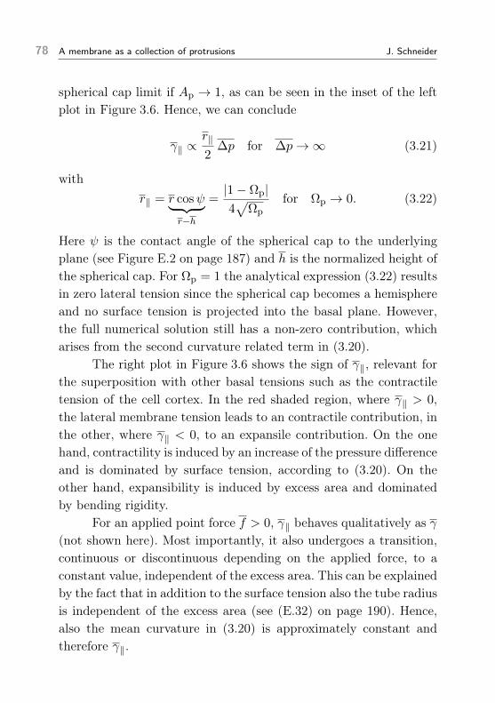
78 A membrane as a collection of protrusions J. Schneider
spherical cap limit if Ap → 1, as can be seen in the inset of the leftplot in Figure 3.6. Hence, we can conclude
γ‖ ∝r‖
2∆p for ∆p→∞ (3.21)
withr‖ = r cosψ︸ ︷︷ ︸
r−h
=|1− Ωp|4√
Ωpfor Ωp → 0. (3.22)
Here ψ is the contact angle of the spherical cap to the underlyingplane (see Figure E.2 on page 187) and h is the normalized height ofthe spherical cap. For Ωp = 1 the analytical expression (3.22) resultsin zero lateral tension since the spherical cap becomes a hemisphereand no surface tension is projected into the basal plane. However,the full numerical solution still has a non-zero contribution, whicharises from the second curvature related term in (3.20).
The right plot in Figure 3.6 shows the sign of γ‖, relevant forthe superposition with other basal tensions such as the contractiletension of the cell cortex. In the red shaded region, where γ‖ > 0,the lateral membrane tension leads to an contractile contribution, inthe other, where γ‖ < 0, to an expansile contribution. On the onehand, contractility is induced by an increase of the pressure differenceand is dominated by surface tension, according to (3.20). On theother hand, expansibility is induced by excess area and dominatedby bending rigidity.
For an applied point force f > 0, γ‖ behaves qualitatively as γ(not shown here). Most importantly, it also undergoes a transition,continuous or discontinuous depending on the applied force, to aconstant value, independent of the excess area. This can be explainedby the fact that in addition to the surface tension also the tube radiusis independent of the excess area (see (E.32) on page 190). Hence,also the mean curvature in (3.20) is approximately constant andtherefore γ‖.

3.4 Combining protrusions to a membrane 79
3.3.3 | Vertical protrusion force
Besides the tension γ‖, which acts laterally to the boundary line,an additional force is acting vertically in z-direction, perpendicularto the boundary line. It is initiated by the pressure difference andthe applied point force f at the protrusion tip. Both would trigger adisplacement of the protrusion in z-direction if it would not be fixedat the boundary. The force contribution from the pressure differenceis given by the product of ∆p with the area projected in the x-y-plane, facing towards the pressure difference. We can expect that thisarea is equivalent to the basal protrusion area Ap‖ (see Figure 3.1).This can be proven by computing∫
dAn · ez = πρ2∣∣l/20≡ Ap‖ . (3.23)
Hence, the total vertical force along the circular boundary line readsas
f⊥ := f +π
4∆p. (3.24)
3.4 | Combining protrusions to a membrane
In chapter 2 we found that a membrane anchored along a squarelattice forms nearly axisymmetric out-of-plane protrusions in eachlattice element if excess area is available. This supports a membranedescription, introduced earlier by Sens et al. [155], where the mem-brane is structured by a collection of disc-like patches, which canbuckle into spherical caps. We extend this concept by using our moreaccurate results for membrane protrusions, including non-vanishingpressure differences and point-forces applied at the protrusion tips.Again, as introduced in chapter 2, we structure the membrane bya square lattice with identical unit elements, as sketched in Figu-

80 A membrane as a collection of protrusions J. Schneider
Figure 3.7 | Membrane structured as a collection of protrusions. a Top view ofthe membrane with one protrusion located in each element of a square lattice. Theprotrusions are anchored along a circle with diameter l (dashed lines). b magnifiesone element of the lattice and its neighbors. It indicates the lipid flow betweenneighboring protrusions, which occurs when their surface tensions differ (see(3.27)).
re 3.7a. Each unit element hosts one axisymmetric protrusion withdiameter l. Along the circumference the protrusion is tightly ancho-red to the underlying plane (dashed circles in Figure 3.7a), where thiscircular binding is the approximation of the actual binding along thesquare lattice. Locally, we characterize each protrusion by an areaApnm , a point force fnm and, in principle, also a spontaneous curva-ture C0nm which we, however, set to zero here. The used indices nand m label the unit elements in x and y directions. Global membra-ne properties, that all protrusions share, are the pressure difference∆p, the bending rigidity κ and the surface tension γ 5. Furthermore,the total area of the membrane can be written as
A =∑n,m
[Apnm + l2
(1− π
4
)]≈∑n,m
Apnm (3.25)
5 Whereas ∆p can, indeed, be seen as a global quantity, κ could, in principle, beintroduced locally for each protrusion to account, e.g., for inhomogeneities in thelateral membrane composition.
3.4 Combining protrusions to a membrane 81
or in case of A → ∞ for an infinitely spread membrane (see forcomparison (2.1) on page 46) the finite excess area
Ω :=A
A‖− 1 =
π
4〈Ωp〉 ≈ 〈Ωp〉. (3.26)
Here A‖ =∑l2 and 〈Ωp〉 is the average excess area per protrusion.
The approximations in (3.25) and (3.26), which we will use in thefollowing, neglect contributions to the area coming from the cornersof the square lattice which are not covered by the protrusion base6.
3.4.1 | Flow equation for the lipid exchange between protrusions
In order to describe the equilibrium state of a membrane, made bya collection of protrusions, we assume that the lipid diffusion wi-thin one unit element is significantly faster than between differentunit elements. One potential explanation for this could be the hopdiffusion, reported previously (see section 1.1.2) [59, 66]. Then theequilibrium shape of a single protrusion is reached almost instanta-neously compared to the global equilibrium shape of the membrane.Therefore, we can treat each protrusion at a given time point du-ring the global equilibration quasi-statically, i.e., as it would havea constant surface area Ωpnm with an associated surface tension, asdiscussed in section 3.3.1. However, since we regard the surface ten-sion as a global quantity of the membrane, only certain area valuesare possible. If we assume an initial non-equilibrium area distributi-on among the protrusions, this can lead to local differences in surfacetensions. These differences, in turn, induce a lipid flow from regionswith lower surface tensions to regions with larger surface tensions
6 Choosing a hexagonal instead of a square lattice would further reduce the errormade by neglecting the non-covered regions.

82 A membrane as a collection of protrusions J. Schneider
and, thereby, trigger an equilibration of the surface tension7. Wedescribe this equilibration by the following linear dynamic ansatz:
α
〈Ωp〉d
dtΩpnm =
∑i,k
γ(Ωpnm)− γ(Ωpn+im+k), (3.27)
where α is a friction coefficient and the summation runs over allneighbors of the lattice element at position n,m.
With the numerical results for γ from section 3.3.1, equation(3.27) forms a set of differential equations for the area distributionΩpnm , which can be solved numerically. Starting from any non-equi-librium configuration, the limit t → ∞ determines the equilibriumdistribution. In the following work, we will always start from a ho-mogeneous distribution, equivalently to the description in chapter2, where each protrusion carries the same area Apnm = Ap and〈Ωp〉 = Ωp = Ω, respectively. This initial configuration is immedia-tely an equilibrium state because the surface tension is a priori iden-tical everywhere. Its value is determined by the pressure differenceand the excess area. An example of such a membrane configurationwith Ω = 0.2 and ∆p = 200 is shown in Figure 3.8a8.
3.5 | Equilibrium area distribution between coupledprotrusions
If we start from an initially homogeneous area distribution, as des-cribed in the previous section, and add a small perturbation to thearea of one protrusion, we find with (3.27) two different characteri-
7 Strictly speaking, the flow of lipids is determined by the bare surface tension γb,introduced in section 1.3.2, for which we assumed here γb ' γ. However, evenwithout this assumption the flow is presumably determined by γ as fluctuationsrenormalize all effective tensions in the same way.
8 For the numerical realization of (3.27) we use periodic boundary conditions.

3.5 Equilibrium area distribution between coupled protrusions 83
a
0
0.5
z
∆p = 200
0
0.5
-1 0 1
x
∆p = 100
b
Figure 3.8 | Equilibrium shapes of coupled membrane protrusions. a shows onepossible equilibrium shape of four neighboring protrusions, arranged on a squarelattice and coupled via (3.27). The excess area is Ω = 0.2 and the pressuredifference ∆p = 200. b shows the equilibrium height profile for two protrusionswith an average excess area 〈Ωp〉 = 0.2 and two different pressure differences ∆p.C 0 = 0, ∆u = 0.01.
stic equilibrium states when we keep the excess area constant butchange the pressure difference. The symmetric homogeneous equili-brium state switches below a certain pressure difference to an asym-metric equilibrium state, i.e., one protrusion assembles more areathan the others (see example with two protrusions in Figure 3.8b).This suggests that, depending on the chosen parameters Ω and ∆p,the homogeneous state can, in fact, become an unstable equilibrium.
To understand this behavior more quantitatively, we study thelinear stability of (3.27). We do this by using the fact that the right-hand side of (3.27) is equivalent to the discrete form of the Laplaceoperator (see appendix D and [185]), where the discretization stepis given by the mesh size ξ ≡ l. Hence, we can write (3.27) approxi-mately as
αd
dtΩpnm ≈ −4‖γ(Ωpnm). (3.28)
We then expand (3.28), including γ(Ωpnm), around the homogeneous

84 A membrane as a collection of protrusions J. Schneider
state Ωpnm = Ωp = Ω what leads to a simple diffusion equation:
dΩ
dt= D4‖Ω with D = − 1
α
∂ γ
∂Ω. (3.29)
The area distribution among the protrusions is then defined by thesign of the diffusion constant D. For D > 0 the diffusion triggers aspreading so that the area is kept distributed homogeneously. D < 0
has the inverse effect, which leads to the observed instability. As thesign of D is defined by the sign of the derivative of γ with respectto Ω, we can conclude that
∂γ
∂AΩ< 0 ⇔ homogeneous state stable. (3.30)
This finding implies that minima in γ(Ω) separate stable from unsta-ble homogeneous states. The surface tension of membrane protrusi-ons and, hence, of a membrane made by those contain such minima,as discussed in section 3.3.1. That is why we can deduce from thissurface tension stability diagrams depending on Ω, ∆p and f 9. In-terestingly, the surface tension for the anchored membrane sheet inweak-bending approximation from chapter 2 does not exhibit suchminima in the area dependency. Instead, its surface tension is al-ways decaying monotonously in Ω and thus a homogeneous areadistribution is always stable. In order to understand the reason forthis significant difference between the two models we calculate inappendix E.1 the surface tension of an axisymmetric protrusion inthe weak-bending approximation. We find that also in this case nominima occur, implying that the difference is not due to the differentmodeling of the anchoring but caused by the weak-bending approxi-mation. We verify this in appendix D where we show that the weak-
9 We do not include the effect of spontaneous curvature here, however, our modelcan account for it.

3.5 Equilibrium area distribution between coupled protrusions 85∆
p[104]
Ω
0.68
3125
0
1
0 0.5 1 1.5
a
∆p[104] Ω = 0.68
Ω
∆L
∆p = 3125
0
1
0
1
-1 0 1
b
Figure 3.9 | Stability of a homogeneous excess area distribution for a collection ofprotrusions. a shows the stability of a homogeneous area distribution amongmembrane protrusions as a function of membrane excess area Ω and normalizedpressure difference ∆p. The red shaded area corresponds to stable configurations.The inset plots show schematically the surface tension γ as a function of the areaand the characteristic position of a stable and unstable point (see text). The reddashed line indicates the transition position for spherical caps, used as an analyticalreference. b shows the transition from a homogeneous area distribution to ainhomogeneous distribution for two coupled protrusions (see also Figure 3.8b). As ameasure for the equality the difference of tip elongations ∆L is used. In the upperplot the transition line is crossed at constant Ω for changing ∆p, in the lower plotat constant ∆p for changing Ω. Their positions within the stability diagram areindicated by blue arrows in a. C 0 = 0, ∆u = 0.01.
bending approximation, in fact, misses nonlinear terms importantfor the calculation of the surface tension.
3.5.1 | Equilibrium area distribution without force perturbations
For zero point force but variable excess area and pressure differencethe surface tension of a protrusion collection contains one minimumin Ω (see Figure 3.5). The position of this minimum depends on ∆p
so that we can find a transition line ∆p(Ω) which gives rise to a sta-

86 A membrane as a collection of protrusions J. Schneider
bility diagram for a homogeneous area distribution shown in Figu-re 3.9a. The stable region, where excess area remains distributed ho-mogeneously, widens with increasing pressure difference and shrinkswith increasing excess area. The maximal excess area, for which astable homogeneous distribution is still possible, can be found in thelimit ∆p→∞ and is Ω = 1. Above this value the homogeneous dis-tribution is always unstable, independent of the pressure difference.This can be interpreted by the previously used spherical cap approxi-mation, since at Ω = 1 the surface tension of caps becomes minimal(see (3.17)). Furthermore, it can easily be shown that above this va-lue a second asymmetric solution for the area distribution betweencaps occurs. This asymmetric solution agrees with our observationin Figure 3.8b for the full shape solution. In Figure 3.9b we quantifythe transition between symmetric and asymmetric state by plottingthe elongation difference between two protrusions for either varyingΩ or ∆p. We find that the transition corresponds to a supercriticalpitchfork bifurcation [193].
For more than two protrusions, located in the unstable regionof Figure 3.9a, an initially homogeneous area distribution collapsesinto a relatively large bleb, in which most excess area is stored, withall other protrusions being relatively flat bulges. This type of blebformation has been reported previousely in a work by Sens et al.to explain membrane shedding of red blood cells [155], which wealso discussed in section 1.4 and at the beginning of section 3.4.They find that the local buckling of membrane into an out-of-planeprotrusion leads always to the formation of a bleb. However, theydid not include a pressure difference across the membrane into theircalculations. As we find, this is required to stabilize the homogeneousarea distribution and prevent blebbing, as described here.
3.5 Equilibrium area distribution between coupled protrusions 87
3.5.2 | Equilibrium area distribution with point forceperturbations
Compared to the previous section, as soon as a non-vanishing pointforce f is applied to all protrusions more than two equilibrium statesfor the area distribution are possible. All possibilities are summari-zed in the shape diagram in Figure 3.10a. For pressure differencesabove the maximal possible for tube formation (see section 3.2.4)the stability behavior is mostly comparable to the case with zeropoint force. Below Ω ≈ 1 the occurring buds are stable, above un-stable, related to bleb formation. However, for pressure differenceswhere tubes can form several stability regions occur as then the areadependency of the surface tension exhibits more than one minimum(see section 3.3.1 and Figure 3.4c). Besides the two stable regionsfor buds and tubes with homogeneous area distributions, two unsta-ble regions occur. One lies in-between the stable regions, and one atlarger excess areas.
The alternation of stable and unstable regions has an intere-sting implication, namely that, in principle, tubes and bulges cancoexist and, at the same time, bleb growth can be limited. This canhappen when the increasing difference of excess area, triggered bythe instability, shifts some of the protrusions into the stable tubestate. There the surface tension is larger than for bulges so that li-pids flow towards the tubes until the bulges have reached an excessarea associated with the same surface tension as the one of tubes.The final equilibrium state would be inhomogeneous, bulges wouldhave a different excess area than tubes. The exact final configurationdepends on the initial value of Ω as well as of ∆p, f and the totalnumber of protrusions. Hence, a more quantitative analysis could gi-ve rise to an extended shape diagram where more membrane statesare distinguishable.

88 A membrane as a collection of protrusions J. Schneider
3.5.3 | Equilibrium area distribution with partial point forceperturbations
Another possibility how both membrane bulges and tubes can oc-cur at the same time is the partial perturbation by a point force f ,i.e., f is applied to only some bulges. In this case, for an initiallyhomogeneous area distribution the surface tensions do not need tobe identical a priori, since they depend differently on Ω for differentpoint forces, as discussed in section 3.3.1. Consequently, a stable ho-mogeneous area distribution exists at the intersection points of allsurface tensions, i.e., in general, only for discrete values of Ω. Howe-ver, also other, inhomogeneous, equilibrium configurations, triggeredby the flow equation (3.27), can allow coexisting tubes and bulges,similarly to what we discussed at the end of the previous section.
Here we study the possible coexistence of such a mixture byusing the analytical limits of spherical caps and cylindrical tubes,as introduced before10. We assume that all tubes are subject to thesame point force f and both tubes and bulges have the same initialexcess area Ωtube0 = Ωcap0
=: Ω0. Since the surface tension of cylin-drical tubes does not depend on the excess area (see, e.g., (3.18)),only the surface tension of caps changes as the equilibrium state isreached and only there stable and unstable regions can be identified.As the inset of Figure 3.10b illustrates, then two equilibrium points,where γtube = γcap, exist, namely
Ω± = 2
(∆pmax
∆p
)21±
√1−
(∆p
∆pmax
)2− 1 (3.31)
10The respective surface tensions can be found in (E.24) on page 188 and in (E.37)on page 192.

3.5 Equilibrium area distribution between coupled protrusions 89
∆p
Ω
100
200
300
400
500
600
700
0 1 2 3 4 5
tubes
bulges
a∆
p/
∆p
max
Ω
∆ptube/∆pmax
∆p/
∆p
max
Ω
∆ptube/∆pmax
1
0 1 2 3
I
II
III
1
0 1 2 3
I
II
III
b
Figure 3.10 | Shape states for a collection of protrusions perturbed by local pointforces. a shows the stability for membrane protrusions to which an external pointforce f = 100 is applied (top left schematic) as a function of the excess area Ω andpressure difference ∆p. The red shaded area corresponds to the stable region. Theinset magnifies the unstable region in the left part of the diagram. The red dashedline marks the transition line from non-tubular to tubular protrusions according toFigure 3.4c. C 0 = 0 and ∆u = 0.01. b shows the stability for a membraneconsisting of a mixture of caps and cylindrical tubes with point force (top rightschematic) as a function of the pressure difference ∆p and the initial excess areaΩ0. The y -axis is normalized according to (3.32). The red shaded regioncorresponds to a stable coexistence of tubes and caps, where the light shaded partindicates a conditional stability (see text). In the gray shaded region only caps canbe persist. In the white region blebs occur and absorb all area from tubes. The reddotted line indicates the critical pressure difference needed to form a tube (see(3.15)) and the numbers correspond to the stability conditions of (3.34) – (3.36).The inset sketches the surface tensions of both protrusion types as a function ofthe excess area and their intersection points. The chosen value for the cap fractionis q = 0.8.
with
∆pmax =f
2
2π2. (3.32)
Assuming a homogeneous area distribution, the equilibrium excessarea of a cap and a tube, respectively, reads as
Ωcap∞ = Ω±, Ωtube∞ =qΩ± − Ω0
q − 1, (3.33)

90 A membrane as a collection of protrusions J. Schneider
where q is the fraction of caps on the total number of lattice elements.From (3.31) and (3.33), we can deduce that tubes only occur in thefinal equilibrium state if the following three conditions are satisfied:
I: Ω0!< Ω+, (3.34)
II: ∆p!< ∆pmax, (3.35)
III: Ω0!> q(Ω− − 1) + 1. (3.36)
The first condition accounts for the stability of caps with respectto each other. For Ω0 < 1 they are stable and, thus, reach Ω− inequilibrium. For 1 ≤ Ω0 < Ω+, caps are unstable and a bleb forms.However, their final state depends on the exact configuration of capsand tubes. One possibility is, since their surface tension is then smal-ler than that of tubes, that they also equilibrate to Ω− before thebleb can grow larger than Ω+. Otherwise, if the bleb can reach Ω+
or if Ω0 > Ω+, the occurring bleb absorbs all area from the tubes.In the context of Figure 3.10a absorption means that they collapseto non-tubular buds, here it simply means that they have no excessarea in the final state. The same happens if the two other conditions,(3.35) and (3.36), are violated. In the first case, i.e., if ∆p > ∆pmax,the surface tension of caps is always larger than that of tubes, whichalso causes the full absorption of tubes. In the opposed case to (3.36),caps absorb all tube area as they approach the equilibrium point Ω−.
We summarize the conditions (3.34) – (3.36) in a shape dia-gram, shown in Figure 3.10b. It reveals that, indeed, for a smallenough pressure difference, ∆p < f
2/2π2, and for sufficiently small
excess area, Ω . 1, caps can coexist with tubes. However, as discus-sed above, an increasing pressure difference triggers the formation ofblebs where tubes disappear.

APPLICATIONS TO CELL BIOPHYSICS 4
Summary: From the general case of a membrane anchored to a sub-strate, as modeled in the previous chapters 2 and 3, in this chapter wefocus on the cell membrane. In this case the membrane is anchoredto the underlying contractile polymeric cell cortex which affects themembrane description in two important ways: First, the anchoring,maintained by linker proteins, can rupture and, thus, the membranecan detach. Second, the pressure difference ∆p = pint − pext bet-ween the inside and the outside of the cell, previously used as a freeparameter, is now coupled to the contractile tension within the cellcortex.
We use our findings from chapter 3 to describe the cell mem-brane as a collection of protrusions. Based on this picture, we intro-duce a closed system of equations for the membrane surface tensionand shape, the pressure difference across the membrane and the cellradius, depending on subcellular parameters for the cell cortex andmembrane and on the cell osmolarity. We can conclude from thisdescription that the membrane buckles into out-of-plane protrusi-ons due to the contractility of the cell cortex. We further discussthe implications of this buckling under different experimental con-ditions. First, we show that an increase of the external osmolaritycan trigger the formation of blebs and tubes as described in the pre-vious chapter. In addition, we study the formation of blebs due to
91

92 Applications to cell biophysics J. Schneider
a local detachment of the membrane from the cell cortex. In thelast part of this chapter we study the membrane behavior duringcytokinesis. We use our membrane model to describe the buckling ofmembrane experimentally observed during cell pole oscillations. Wederive an equation for the flow of membrane through the cleavagefurrow, triggered by these oscillation. From a preliminary compari-son to experimentally measured fluorescence data of the membranewe estimate the buckling state of the membrane prior pole oscilla-tions. Moreover, we show that the cell membrane itself could alsoinfluence the oscillations by introducing a surface elasticity, arisingfrom the local membrane buckling.
4.1 | The cell membrane as a collection of protrusions
In this chapter we consider the cell membrane as a lipid bilayer, en-closing the biological cell, anchored to the underlying cell cortex vialinker proteins. It is subject to a pressure difference ∆p between cellinside and outside and can locally be exerted into tubular structuresby a force f induced by spiking cortical filaments pushing against themembrane. The filamentous structure of the cortex compartmentali-zes the membrane as it attaches to it by multiple linker proteins andforms a fence-like structure (see section 1.1.2 for further details onthe cell membrane). We assume here, for simplicity, that this com-partmentalization can be idealized by a square lattice with equallysized unit elements as shown in Figure 4.1a.
Based on these assumptions we follow our work in chapter 3 bytreating the membrane in each lattice element as an axisymmetricprotrusion. Each protrusion has the same diameter lp which is equalto the mesh size ξ of the lattice. We always start in the followingfrom a homogeneous area distribution, i.e., the excess area of eachprotrusion is identical to the overall cell membrane excess area, Ωp ≡

4.1 The cell membrane as a collection of protrusions 93
Figure 4.1 | The cell membrane as a regular mesh of protrusions with axialsymmetry. a shows a sketch of the simplified structure of the cell membrane shapeas assumed here. In b the different occurring physical forces are summarized: Thelateral membrane tension γ‖ and the active contractile tension T in the cell cortexsum to an overall (contractile) tension which is balanced by the pressure difference∆p. As a consequence, at each linker between membrane and cortex a force dipoleis induced, as already discussed in chapter 2 (see also Figure 2.2 on page 48 forcomparison). In addition, cortical filaments can locally exert a force f on themembrane which can then form a thin tube. The magnified region emphasizes therelation between the absolute membrane area Ab, stored in fluctuations, and theeffective area A (see also section 1.3.2).
Ω. The apparent surface area S = 4πR2 of the cell, with R beingthe cell radius, is assumed to be approximately equal to the sumof all basal protrusion areas (see approximation (3.26) on page 81).Furthermore, we assume a protrusion size that is small compared tothe cell size, i.e.,
l
R 1. (4.1)
Then the cell curvature is negligible for individual protrusions.With (4.1) we can use, in good approximation, our results from
chapter 3 for a flat anchored membrane, modeled as a collection ofprotrusions. This includes, in particular, the surface tension γ and

94 Applications to cell biophysics J. Schneider
lateral tension γ‖, which we obtained by solving the shape equations(3.6) and (3.7) on page 64 at a constant protrusion area and thenallowed the equilibration of γ to a global value among all protrusionsvia lipid exchange according to (3.27) on page 82. As we found, γand γ‖ only depend on lp, Ap, ∆p and f . In the following we changethe variables from
lp,Ap → R,A (4.2)
by using the relations1
A ' NpAp, R '√Np
4lp. (4.3)
Here Np is the number of protrusions which we assume to be fixedfor a given cell, determined by the mesh of the cell cortex.
4.2 | Cell mechanics based on the membrane-cortexinterplay
4.2.1 | Closed description of the membrane-cortex interplay
As the cell membrane is anchored to the contractile cell cortex we ex-pect a mechanical interaction between both and therewith a feedbackon the overall cell mechanics. In order to describe this interactionwe propose here a closed system of equations which combines sixfundamental relations for the geometrical and mechanical state ofmembrane and cortex.
The first relation is given by (1.10) on page 32. It states howmuch total membrane area Ab, stored in fluctuations, is visible asthe effective, accessible, membrane area A (see Figure 4.1b). This
1 We ignore here the area contributions coming from the corners of the squarelattice which are not covered by the protrusion base (see section 3.4 for details).

4.2 Cell mechanics based on the membrane-cortex interplay 95
depends on the surface tension γ of the membrane and reads as
A = A(γ,Nl) = Nlπρ2l
[kBT8πκ
log
(κq2
max + γ
κq2min + γ
)+ 1
]−1
. (4.4)
Here Nl is the number of lipids inside the membrane, which we as-sume to be fixed. The lipid number is related to Ab via the charac-teristic lipid surface radius ρl as Nl = Ab/πρ
2l . For the minimal and
maximal fluctuation modes in (4.4) we assume qmin = π/lmem ∼2π µm−1 and qmax = π/lmic ∼ 200π µm−1, where we have usedlmic ∼ 5 nm (the characteristic length scale of the membrane, e.g.,its thickness) and lmem ∼ 500 nm (the characteristic mesh size of thecell cortex, see section 1.1.1)2.
The second relation follows by taking into account the balanceof chemical potential of water between cell inside and outside. Thenthe pressure difference ∆p is equival to the osmotic pressure diffe-rence Πint − Πext. With the help of Van’t Hoff’s relation [194, 195]we can rewrite the internal osmotic pressure of the cell Πint by theratio of solute molecules in the cell Nint to the total cell volume3.Hence, we find the relation
∆p = ∆p(R,Vp,Np,Nint, Πext) = kBTNint
43πR
3 +NpVp−Πext (4.5)
Here the total cell volume is the sum of the volume enclosed by thecell cortex at radius R and the volume underneath each protrusionVp, where the latter we assume to be identical for all protrusions (seesection 4.1).
The third relation is given by the force balance between out-ward pointing pressure difference ∆p and the inward pointing stress
2 In fact, the minimal mode depends on the basal diameter of each protrusion andthus on R. For simplicity, we ignore this here.
3 Van’t Hoff’s relation reads as Π = kBT NV.

96 Applications to cell biophysics J. Schneider
σtot at the cell surface (see Figure 4.1b). This inward pointing stresswe obtain by superposing the active contractile cortex tension T withthe lateral membrane tension γ‖. The result read as
∆p = ∆p(R, γ‖,T ) = 2T + γ‖
R︸ ︷︷ ︸σtot
, (4.6)
where the right-hand side is the extension of Laplace’s law (see (1.2)on page 27). The active tension T is generated by motor proteins inthe cell cortex, which exert local forces on the polymeric network. Ina very simple model, as stated in (1.1) on page 22, it can be assumedthat T ∝ cm, where cm is the concentration of myosin motors.
All three relations (4.4) – (4.6) contain information on thebuckling state of the membrane, (4.4) via the surface tension γ, (4.5)via the volume enclosed by a membrane protrusion Vp and (4.6) viathe lateral membrane tension γ‖. To express the quantities γ, γ‖and Vp we use our results from chapter 3 where we computed themnumerically by solving the shape equations (3.6) and (3.7) on page64 for axisymmetric protrusions4. From this we can deduce threemore relations for the membrane-cortex description, determining themechanics and geometry of membrane buckling. In general terms wecan write them as
Vp = Vp(R,A, ∆p, f ,Np), (4.7)
γ = γ(R,A, ∆p, f ,Np), (4.8)
γ‖ = γ‖(R,A, ∆p, f ,Np). (4.9)
We now assume that the parameters Nl, Np, Nint, Πext, T
4 The surface tension γ is computed simultaneously with the equilibrium shapevia (3.10) on page 65, γ‖ from (3.20) on page 77 and Vp from the volume formulain Table B.1 on page 150.

4.2 Cell mechanics based on the membrane-cortex interplay 97
and f are known. Here Nl, Np, T and f are those parameters de-scribing the state of the coupled membrane-cortex layer. Moreover,the latter three contain, implicitly, further details on the cell cortexconfiguration itself, e.g., its network geometry and local force gene-rations, which are, in turn, related to the number and activity ofother molecules, for instance of actin, myosin and cross-linker pro-teins. With this knowledge, the six relations (4.4) – (4.9) become aclosed system of equations for the four geometrical quantities cellradius, membrane area, cell volume and protrusion volume, and thethree mechanical quantities, pressure difference, surface tension andlateral tension:
Nl,Np,Nint, Πext,T , f(4.4) – (4.9)
=⇒ R,V ,A, ∆p, γ, γ‖,Vp. (4.10)
Thus, the closed equation system determines the mechanical andgeometrical state of the cell self-consistently by underlying subcel-lular parameters of the cytoskeleton and the membrane and by thecell osmolarity. In particular it determines the pressure difference∆p, the membrane area A and the protrusion diameter lp, whichwe used as free parameters in the previous chapters. Also the radiusR, which marks the position of the cell cortex, is here no longer afree parameter5. Furthermore, we assume the following approximatevalues for the subcellular parameters on the left-hand side of (4.10):The tension T is of the order of 100 pN/µm [16,24]. The local pointforce f is of the order of 10 pN/µm [196,197]. The external osmoticpressure Πext is of the order of 106 Pa for typical osmolarities (molarconcentrations) in biological solutions [198]. With an assumed cellradius of R ∼ 5µm this implies Nint ∼ 1011. Nl and Np can be esti-mated from the cell radius, the respective apparent cell surface areaS, the radius of a lipid, ρl ∼ 0.5 nm [9], and the membrane anchoring
5 We here consider the cell to be at steady-state so that the cell cortex has alreadyadopted this radius.

98 Applications to cell biophysics J. Schneider
mesh size, ξ ∼ 500 nm, respectively. Then Nl ∼ 106 and Np ∼ 1000.The proposed self-consistent description of the coupled mem-
brane-cortex layer is, to our best knowledge, the first that connectsthe global mechanical and geometrical state of a cell to subcellu-lar parameters. Although other mechanical models for cells, basedon cortical tension superposed with the membrane surface tension,have been proposed before (e.g., in [154]), our approach includes,for the first time, the out-of-plane shape, and the resulting bucklingmechanics, of the membrane.
4.2.2 | Self-consistent solution for the membrane-cortexinterplay
To solve the closed system of equations (4.4) – (4.9), we ignore fornow the effect of cortical filaments pushing against the membrane,i.e., we assume f = 0. At the same time, we ignore local forces thatapply to individual anchoring points between membrane and cortex.Furthermore, we neglect effects arising from the flow between pro-trusions (see section 3.4) and consider all protrusions to be identical,with the same basal diameter and excess area. We will discuss theeffects of local forces exerted to the membrane and membrane flowin the context of bleb and tube formation in section 4.3.
For a vanishing cortical tension, T = 0, the closed system ofequations (4.4) – (4.9) can be solved analytically, as we show inappendix G. The result is a round cell shape with the membranebeing tightly attached to the underlying cell cortex. This implies thefollowing relations:
A0 = 4πR20, V0 =
4
3πR3
0, ∆p0 = 2γ0
R0. (4.11)

4.2 Cell mechanics based on the membrane-cortex interplay 99
Furthermore, γ0 can be expressed as a function of R0:
γ0 =3kBT Nint − 4πR3
0 Πext
8πR20
(4.12)
and R0 itself is defined via the implicit relation
Nlρ2l
4R20
= 1+kBT8πκ
log
[3kBT Nint + 8πκq2
maxR20 − 4πΠextR
30
3kBT Nint + 8πκq2minR
20 − 4πΠextR3
0
]. (4.13)
Hence, the value of R0 depends on two effects, the pressure differencearising from the number of solute molecules inside the cell Nint andthe outer osmotic pressure Πext and the membrane area stored influctuations. In the limit of Nint → ∞, with a finite value of Πext,all fluctuations disappear and R0 → ρl
√Nl/2. Whereas R0 remains
strictly positive for any values of Nint and Πext, γ0 and therewith∆p0 can become negative. The biological implications of both, anegative surface tension and a negative pressure difference, are notfully understood yet. However, there is evidence that for most condi-tions negative surface tensions destabilize the persistent membraneshape leading to spontaneous membrane shedding [199–201]. Smallnegative pressure differences might be resisted by inverted membra-ne buckling and the corresponding energy cost due to curvature butlikely lead to a collapse of the cell above a critical value. That is why,and since we only studied the membrane mechanics for ∆p > 0 inthe previous chapters, we only consider positive pressure differencesin the following. To ensure ∆p > 0 we choose the initial ratio of Nint
and Πext for T = 0 with the help of (4.12) accordingly.For non-vanishing contractile cortex tensions, T > 0 the equa-
tion system (4.4) – (4.9) can, in general, only be solved numerically,as described in appendix G. The results for the above discussed pa-rameter values are shown in Figure 4.2. The first interesting resultis that the pressure difference ∆p differs significantly from the term

100 Applications to cell biophysics J. Schneider
∆A/
A0
T [pN/µm]
Nl01.01Nl0
∆V/
V0
Nl01.01Nl0
∆R/
R0
Nl0
1.01Nl0
0%0.5%
0 500 1000 1500 2000
-0.1%
0%-0.4%
-0.2%
0%
a
1−
2T/
R∆
p
T [pN/µm]
Nl0
1.01Nl0
γ
Nl0
1.01Nl0
00.20.40.60.81
0 500 1000 1500 2000
0
200
400
600
Ω
T [pN/µm]
Nl0
1.01Nl0
Nl/Nl0 buckling
0
0.02
0.04
0 500 1000 1500 2000
0
0.1
1 1.05 1.1
b
Figure 4.2 | Global cell parameters determined through the interplay of cellmembrane and cell cortex. The left plots in a show the numerical results for therelative changes of cell radius R, volume V and area A upon change of cortextension T . R0, V0 and A0 are the reference values at T = 0 (see (4.11) and(4.13)). The right plots in a show the surface tension γ and the ratio of Laplace’slaw 2T/R with the full pressure difference ∆p as a function of T . b shows theincrease of excess area due to membrane buckling for increasing tension andincreasing lipid number (inset plot). All plots are shown for two different lipidnumbers, Nl0 = 1.6 · 109. The other parameters are chosen as Πext = 106 Pa,Nint = 1.29 · 1011, qmin = 2π µm−1, qmax = 200π µm−1, κ = 20 kBT , ρl = 0.25 nm,Np = 1000, f = 0. The schematic on the lower right illustrates how membranebuckling is affected by an increase of cortex tension and lipid number, respectively.

4.2 Cell mechanics based on the membrane-cortex interplay 101
2T/R, coming from the cortex tension (Figure 4.2a). At T = 0 thedeviation is maximal as ∆p is fully determined by the surface tensionγ0. For larger T the deviation decreases. However, even for relativelylarge tensions (T = 2000 pN/µm) it differs by approximately 20 %.This indicates that the contribution from the lateral membrane ten-sion to the force balance (4.6) is not negligible for the mechanicsof a cell. The found order of magnitude for the contribution agreeswith previous experimental estimates [166, 202]. That the contribu-tion does not vanish even for large cortex tensions is due to the factthat we assume a constant bare membrane area Ab so that γ itselfis a function of ∆p. If we recall the approximate analytical result forthis relation from our membrane model in chapter 3, γ ∼ ∆p, (see(3.21) on page 78), we find the asymptotic relation
∆p ∝
[1− 4√
Npr‖
]︸ ︷︷ ︸
≥1
−12T
Rfor T →∞. (4.14)
The second important observation we can deduce from Figu-re 4.2b is the buckling of membrane. Whereas for T = 0 the mem-brane is tightly attached to the spherical cell cortex, it starts to formsmall out-of-plane protrusions for T > 0, associated with an incre-asing excess area of the cell. Since a sphere and only a sphere hasminimal surface area for a given volume [203] the observed buckling,starting from a spherical shape, requires a finite volume or surfacearea elasticity. We have accounted for both elasticities by including(4.4) and (4.5) to our description. We can estimate the magnitude ofthese elasticities by linearizing (4.4) and (4.5) around the sphericalstate at T = 0:
γ ≈ γ0 +KAA−A0
A0, (4.15)

102 Applications to cell biophysics J. Schneider
∆p ≈ ∆p0 +KVV − V0
V0. (4.16)
Here KA is the surface area elasticity and KV the volume elasti-city whose expressions we provide in appendix G. For the parame-ters used in Figure 4.2 and Nl = Nl0 = 1.6 · 109 we find KA ≈3.2 · 106 pN/µm and KV ≈ −1.3 · 107 Pa. The different signs of bothconstants imply that both an increase of the surface tension, γ > γ0,and an increase of the pressure difference, ∆p > ∆p0, induces excessarea because in the first case the effective membrane area increases,A > A0, and in the second case the cell volume decreases, V < V0.Hence, also an increasing cortex tension induces excess area, as it in-creases ∆p according to (4.6) and also indirectly γ. However, the ma-gnitudes of KA and KV are relatively large in comparison to typicalvalues of γ ∼ 100 pN/µm and ∆p ∼ 100Pa in cells [166,202]. That iswhy the relative changes of V and A are with a value of approximate-ly 0.1 % very small for the chosen parameters (Figure 4.2a) and onlylittle excess area is stored in membrane protrusions (Figure 4.2b).Interestingly, the buckling effect becomes more significant when thebare membrane area is slightly increased by adding more lipids tothe membrane (inset of Figure 4.2b). For choosing Nl = 1.01Nl0 , thearea elasticity drops to KA ≈ 2.0 pN/µm. This elasticity decreasecan be understood by the fact that more membrane area encloses alarger volume so that for a fixed number of solute molecules Nint thepressure difference decreases6. This, in turn, leads to a decrease ofsurface tension and thus more membrane stored in fluctuations.
The discussed relation between membrane surface tension andmembrane buckling could provide a better understanding of how themembrane actually regulates its surface tension. More precisely, ourfindings indicate that the membrane buckling could be a mechanism
6 Similarly, ∆p would decrease for a constant lipid number but reduced solutemolecule number.

4.3 Membrane blebs and tubes 103
for the cell to reduce its surface tension and, at the same time, pro-vide membrane excess area that can be used to buffer spontaneouscell shape changes.
4.3 | Membrane blebs and tubes
With the help of the self-consistent description for the interplay ofcell membrane and cortex, introduced in the previous section, wecan make predictions under which conditions a cell membrane exhi-bits characteristic out-of-plane structures, namely membrane tubes,invaginations and blebs. We can do this because the self-consistentdescription links subcellular cell properties (left-hand side of (4.10))via the mechanical cell state, mainly determined by ∆p and γ, tothe underlying mechanisms, causing these out-of-plane structures.
4.3.1 | Blebbing and tubulation caused by cortical filaments andlipid flow
We ignored for the self-consistent solution in section 4.2.2 the mem-brane flow and a possible point force at protrusion tips coming fromcortical filaments pushing locally against the membrane. However,as we showed in section 3.5, these two effects trigger the formation ofmembrane blebs and membrane tubes (microvilli). Tubes form whenthe force is large enough to elongate a protrusion bulge, blebs whenthe membrane surface tension promotes an accumulation of lipids inone protrusion, destabilizing a homogeneous area distribution. Wefound that the position of the different transitions is defined by thethree parameters membrane excess area Ω, normalized pressure dif-ference ∆p and normalized point force f (see Figure 3.9a on page85 and Figure 3.10a on page 89). As introduced in the beginning ofchapter 3, the normalizations of the pressure difference ∆p and of

104 Applications to cell biophysics J. Schneider
the force f contain the protrusion diameter lp. This, in turn, de-pends on the cell radius R via (4.3). Hence, for given cell radius andpoint force, the formation of the considered tubes and blebs is fullydetermined by Ω and ∆p. However, in experiments there is usuallyno direct control of these two quantities. Instead common controlparameters are the external osmotic pressure Πext and the cortextension T 7.
Qualitatively, according to our findings in section 4.2.2, weexpect that T mainly affects ∆p, whereas Ω is mostly influenced byΠext. Ω also increases with increasing T , as we discussed, however,for a given contractile tension T > 0 deswelling the cell has a largereffect. This can be achieved by either increasing the bare membranearea, as discussed in section 4.2.2, or by increasing Πext, as discussedhere. Quantitatively, we relate the computed values for Ω and ∆p
where the transitions to tubes and blebs occur to values for T andΠext by the following procedure: First, we calculate R as a functionof Ω, ∆p and f . It is given implicitly by the fluctuation relation (4.4)where we replace γ by (4.8). Second, having R, we solve (4.5) and(4.6) for Πext and T , respectively. The obtained relations
Πext =
√Np
320πR3
[12Nint√Np + 12Vp
− 5π∆p κNp
], (4.17)
T =κNp
128R2
[∆p√Np − 8γ‖
](4.18)
depend only on given subcellular parameters and via R, Vp and γ‖on Ω, ∆p and f . Here Vp and γ‖ are determined by our membranemodel, according to (4.7) and (4.9). Hence, (4.17) and (4.18) directlymap the transition from Ω and ∆p values to Πext and T values,assuming a fixed point force f . The resulting transition lines (lines i
7 The cortex tension can be modified by myosin inhibitors as e.g. Blebbistatin [204]
4.3 Membrane blebs and tubes 105
and iii) are shown in the shape diagrams of Figure 4.3 for f = 0 pNand f = 20 pN.
For a potential experimental comparison the most importantresult is that for a constant tension an increase of the external os-molarity, i.e., the deswelling of the vesicle, can trigger the formationof blebs, on the one hand, and of cortex driven tubes on the otherhand. The latter transition, however, occurs only for small enoughcortex tensions below T ≈ 1000 pN/µm. This limiting tension is ofthe order of typical tensions in biological cells (see section 1.1.1) sothat, in principle, it should be possible to observe the transition ex-perimentally. Furthermore, we find that an increase of tension canstop blebbing if the external osmotic pressure is small enough, hereΠext ≈ 2 · 107 Pa. Both the prevention of tubes and blebs towardslarger tensions seems to be counterintuitive at a first glance. Inde-ed, above a critical value tension can also cause blebbing, namelyby local membrane detachment from the cortex (transition line iiin Figure 4.3), as we will discuss in the next section. However, theblebbing mechanism discussed here, caused by membrane flow, is sta-bilized by tension. In case of tubes our finding is owed the fact thatwe assume the force f of one cortical filament to be uncorrelated tothe tension and therefore to the concentration of motor proteins. Ifwe would impose a relation between f and T , likely, the tube regionin Figure 4.3b would extend towards increasing tensions.
To visualize the relation between Ω, ∆p and T , Πext, we addedto Figure 4.3a dotted lines indicating the position of constant excessareas and constant pressure differences. The excess area scales, asexpected, in good approximation linearly with the external osmoticpressure. The pressure difference, on the other hand, depends onboth T and Πext for most values. In the limit T → 0 it only dependson Πext, according to (4.12) and can be both positive and negativeas also the surface tension can be (red dashed line in Figure 4.3a).

106 Applications to cell biophysics J. Schneider
T[pN/µm]
Πext [107 Pa]
f = 0 pN
0
200
400
600
800
1000
1200
1400
1.5 2 2.5 3
γ > 0γ < 0
i
ii
aT
[pN/µm]
Πext [107 Pa]
f = 20 pN
0200400600800
1000120014001600
2 3 4 5 6 7 8
i ii
iii
b
Figure 4.3 | Theoretical prediction for cell blebbing and cortex driven tubulation.a shows the formation of blebs as a function of external osmotic pressure Πext andcortex tension T . The red shaded region corresponds to a stable area distribution(see section 3.5). In the white region blebs can occur due to two different effects:The transition line i marks blebbing due to membrane flow, as discussed in section4.3.1. The transition line ii marks blebbing due to local membrane detachment, asdescribed in section 4.3.2. The assumed rupturing force is fr = 20 pN and thenumber of anchors per protrusion na = 5. The red dashed line indicates where thesurface tension γ changes its sign. The thin dotted lines correspond to constantpressures (from bottom to top: ∆p = 0, 400, 800, 1200) and constant excess areas(from left to right: Ω = 0, 0.3, 0.6), respectively. In b an additional point force,generated by cortical filaments pushing against the protrusions tips from the cellinside, is included. The additional region, where tubes form (transition line iii), isshaded light red. The other parameters for a and b are chosen as in Figure 4.2 withNl = 1.6 · 109.
Then also the excess area does not depend on Πext any longer, sincethe cell is perfectly spherical with Ω = 0.
4.3.2 | Blebbing and tubulation caused by the discretemembrane anchoring
Another aspect we ignored for the self-consistent solution in secti-on 4.2.2 is the contractility-driven exertion of local forces at eachanchoring point between cell cortex and cell membrane. The con-
4.3 Membrane blebs and tubes 107
tractile stress 2T/R is pulling on the linker proteins, whereas theopposed positive pressure difference is pushing against the membra-ne, both together leading to force balance expressed by a force dipoleas shown in Figure 4.1 (see also the discussions in sections 2.1, 2.3.2and 3.3.3). The related resistive force per linker can be deduced fromthe protrusion force (3.24) on page 79:
fa =8πRT
Npna, (4.19)
where the pressure difference is here replaced by the active stress andna := Na/Np is the number of anchors per protrusion8. The force fagives rise to a second type of blebbing, besides the one presented inthe previous section, caused by a local membrane detachment fromthe underlying cortex. This can happen when fa exceeds a criticalrupturing force [149,165]
fr = const. , (4.20)
which we assume to be constant and determined by protein bindinginteractions. For cells fr is typically of the order of tens of piconewton[149,205].
Alternatively to the detachment, the membrane can also in-vaginate locally into the cell, a process that could be associated toendosome formation [206]. We expect this to happen when, first, acortical filament is anchored almost perpendicular to the membra-ne and, second, when the filament pulls with a force large enoughto buckle the membrane inwards and to form a tube. A first orderapproximation for the force required to pull such a tube is given by
8 na is identical to 2q + 1 anchors per lattice element as introduced in chapter 2.

108 Applications to cell biophysics J. Schneider
the force needed to maintain a tube (see (3.18) on page 76):
ft ≈ 2π√
2κγ . (4.21)
By combining the two effects, membrane detachment and in-vagination, we can distinguish the following four regimes:
I: fa< ft & fa < fr, (4.22)
II: fa> ft & fa < fr, (4.23)
III: fa> ft & fa > fr, (4.24)
IV: fa< ft & fa > fr. (4.25)
For condition I we expect the membrane to remain anchored to theunderlying cortex as described before. In case of condition II themembrane forms tubular invaginations and in case of condition IIIand IV blebs, caused by detachment from the cortex. The transitionlines, which separate these regions, can be found by setting fa = frand fa = ft. We solve both relations for the number of anchors perprotrusion
n(r)a =
8πRT
Npfr, (4.26)
n(t)a =
4RT
Np√
2κγ. (4.27)
Plugging our self-consistent solution from section 4.2.2 for R(T ) andγ(T ) into (4.26) and (4.27), we can express na as a function of Tonly. The inverse T (na) gives the critical tension above which inva-ginations and detachment can occur. The resulting shape diagramis shown in Figure 4.4a, based on the parameters used in Figure 4.2(Nl = 1.6 · 109) and for an assumed rupturing force fr = 40 pN. Theshape diagram reveals that there is indeed a separate parameter ran-

4.3 Membrane blebs and tubes 109
ge where, according to the conditions (4.22) – (4.25), only tubularinvaginations can occur. On the one hand, the corresponding cor-tex tension lies between T ≈ 200 pN/µm and T ≈ 1000 pN/µm andis thus of the order of typical cellular values. On the other hand,for a given cortex tension, the corresponding range of anchors perprotrusion for which invaginations can occur, is relatively narrow(∆na < 1) and above a certain value invaginations cannot occuranymore. We find that the value of this upper limit is mainly defi-ned by the rupturing force fr and the excess area Ω of the membrane.It increases with both increasing fr and increasing Ω. However, forvalues fr ∼ 10 pN and Ω . 0.01 the upper limit appears at relativelysmall values, na . 5 9. Based on these findings, we conclude that thedescribed formation of tubular invagination is presumably rather arare event in cells that requires a relatively low number of about fivelinker proteins per protrusion10. In contrast, the occurrence of blebsis much more dominant. It can happen, in principle, for any value ofna above a critical tension (regions III and IV in Figure 4.4a). Fora given value of na, this critical tension gives rise to an additionaltransition line (line ii) in the shape diagrams Figure 4.3a and Fi-gure 4.3b, below which outward pointing tubes and blebs occur asdiscussed in the previous section and above which blebs caused bythe described local detachment appear11.
In a recent collaboration with the group of Andreas Bauschand there in particular with Etienne Loiseau12 we used the force de-scription above to characterize the blebbing observed in a novel type
9 See for visualization of this anchoring number Figure 2.2 on page 48 (q=2).10This result suggests that other mechanisms that trigger endocytosis, such asspontaneous curvature induction, could be more efficient and thus more favorablefor cells.
11Note that the transition line ii in Figure 4.3 depends on the external osmoticpressure Πext because the cell radius R, entering (4.19), changes with Πext.
12Biophyics Division, Faculty of Physics, Technische Universität München, Ger-many.

110 Applications to cell biophysics J. Schneider
TpN/µm
na
200
400
600
800
1000
1200
1400
1600
1800
2000
1 2 3 4 5 6
III IV
II I
a1 μM anilin 2 μM
0 μ
M
m
yosin c
once
ntr
atio
n
1
μM
NiNTAmembrane
myosin
actin
anilin
b
Figure 4.4 | Membrane perturbations caused by local anchoring forces. a showsthe theoretical prediction of local membrane invaginations and bleb formation dueto detachment of the membrane from the underlying cortex as a function of thecontractile cortex tension T and anchor number per protrusion na. In the redshaded region blebs occur, in the light shaded region tubular invaginations occur,otherwise the vesicle shape is round, covered by small protrusions of equal excessarea. The indicated numbers correspond to the regions introduced in (4.22) –(4.25). The theoretical lines are calculated according to the self-consistent solutionin section 4.2.2, with the same parameters as in Figure 4.2. The used rupturingforce is fr = 40 pN. b shows experimental images of an in-vitro active membranevesicles for different amounts of myosin (1µM ≈ 602 particles/µm3) and anilin(further description see text). The other vesicle parameters are identical: actinconcentration cac = 10µM, NiNTA concentration 10%.Images are taken with abright-field and confocal microscope. Scale bar: 20µm. [Images provided byEtienne Loiseau, Technische Universität München].
of in-vitro membrane vesicles [207]. These vesicles are filled with across-linked actin network which is put under active stress via myo-sin motor filaments. Moreover, the network is bound to the outervesicle membrane via anilin proteins, which bind to NiNTA recep-tors, present in the membrane. A schematic as well as a confocal

4.3 Membrane blebs and tubes 111
image of such a vesicle is provided in Figure 4.4b. Also shown thereare vesicles at different myosin concentration (0µM, 0.5µM, 1µM)and anilin concentrations (1µM, 2µM). An increase of the myosinconcentration is associated to an increase of the active stress in thevesicle, an increase of the anilin concentration to a higher ancho-ring density between actin network and membrane. As the examplevesicles in Figure 4.4b indicate, it systematic experimental analy-sis reveals that a change from intermediate myosin concentrations(0.5µM) to large myosin concentrations (1µM) induces bleb forma-tion of the initially round vesicle, caused by a local detachment of themembrane from the actin network. For a low enough anchoring den-sity this detachment leads, eventually, to a complete collapse of thecontractile actin network (Figure 4.4b top left). For larger anchoringdensity the network does not collapse, only a localized bleb occurs(Figure 4.4b top right). These observations agree qualitatively withthe dependency on na of the transition line shown in Figure 4.4a.As both conditions lead to blebbing the one with the larger ancho-ring density is closer to the transition line. This could explain thesmaller bleb since we expect according to previous work that blebscan releases pressure [166] and thus can trigger a stabilization of thenetwork-membrane anchoring, here by moving down in the shapediagram Figure 4.4a.
With the help of the discussed experimental observations wecan give a quantitative estimate of the rupturing force magnitu-de in such vesicles. We do this by setting fr = fa and replacein the expression (4.19) of fa the contractile tension by and acti-ve stress σ = 2T/R and furthermore the total anchor number byNa = 4πR2/l2a, where la is the mean distance between anchoringpoints. We then find
fr = 2σl2a. (4.28)
We can estimate σ from the myosin concentration via the relati-

112 Applications to cell biophysics J. Schneider
on σ ' fmf lmfcm/nmf (see section 1.1.1). The length of a myosinfilament is approximately lmf ≈ 1µm in the vesicle, with 100 mo-tors participating in one filament. The force of a filament is of theorder of fmf ≈ 20 pN, i.e., a myosin concentration of 1µM, as requi-red for bleb initiation in vesicles, corresponds to a stress of aboutσ ≈ 120Pa. The mean anchor distance can be estimated experi-mentally by analyzing intensity profiles of the anilin distributionwithin the vesicle [207]. For vesicles with an anilin concentrationcan = 0.2µM the distance is of the order of la ≈ 36 nm. Hence, wefind fr ≈ 0.3 pN, which is approximately two orders of magnitudesmaller than the force measured in cells [149]. The reason for sucha large difference could be that in cells the anchoring is achieved bya much more complex interplay of different linker proteins [45, 208]than in the vesicle. Cells might favor such strong binding in order toguarantee an intact connection between membrane and cortex for alarge range of contractile tensions and to avoid a complete membranedetachment as observed for the described vesicles.
4.4 | Cell membrane mechanics during cytokinesis
4.4.1 | Membrane buckling due to cell pole contractions
As a consequence of Laplace’s instability cell pole oscillations canoccur during cytokinesis, the last stage of cell division (see secti-on 1.2 and [26]). Recent observations of the cell membrane duringthese oscillations, presented in section 1.4, have revealed that themembrane buckles on the contracted pole and appears relatively flaton the expanded. A supporting illustration of this membrane out-of-plane structuring is shown in Figure 4.5. Experimentally it hasbeen verified that the volume of the cell during cytokinesis is con-stant [26, 209]. Furthermore, also the surface area of the membrane

4.4 Cell membrane mechanics during cytokinesis 113
cell membrane
linkerprotein
Figure 4.5 | Cross section of a cellduring cytokinesis. The left sideshows a part of Figure 1.6 (confocalimage of the fluorescently labeled cellmembrane, intensity inverted). Theright part illustrates the expectedshape of the membrane. R1 and R2,S1 and S2, A1 and A2 are the radii,apparent areas and membrane areasof the two cell poles, respectively. Rcis the radius of the cleavage furrow.
seems to be conserved, an observation we will further discuss in 4.4.2.With these two conservations, the remaining equations of the closedsystem of equations in section 4.2.1 are (4.6), (4.8) and (4.9). Theyimply that the Laplace pressure in (1.2) on page 27, driving the os-cillations, must be extended by a contribution from the membrane.In general, we can write
α
Vs
dV1
dt= − α
Vs
dV2
dt≡ α
2
dV12
dt= −∆p12, (4.29)
where ∆p12 := ∆p1 −∆p2 and V12 := (V1 − V2)/Vs13.
We can understand the observed buckling during cell pole os-cillations in a first simple approach with the help of our membranemodel of section 4.1 and the assumption that the membrane area ofeach pole remains constant, i.e., the cleavage furrow acts as a dif-
13Vs is the pole volume in case of symmetric poles, as introduced before.

114 Applications to cell biophysics J. Schneider
fusion barrier for lipids. The buckling is then simply caused by thecontraction of the anchoring lattice, due to the decrease of the cellpole volume. We can estimate the effect of contraction by assumingthe following further simplifications: First, the cell poles are appro-ximately portions of spheres, which connect at the cleavage furrowwith constant radius Rc (see Figure 4.5). Second, the geometry ofthe anchoring lattice remains unchanged, implying that the numberof protrusions Np is constant on each pole during oscillations. ThenNp can be computed by the mesh size ξi and the apparent surfacearea Si on either pole via Np = 4Si/πξ
2i . Last, the volume contribu-
tion coming from the protrusions is taken to be negligible comparedto the total cell volume. Subsequently, Ri and ξi can be related asfollows14:
ξi = Ri
√√√√ 8
Np
(1 +
√1− R2
cR2i
). (4.30)
Hence, with characteristic values for the furrow radius and radius Rs
and mesh size ξs in case of symmetric poles we can estimate Np andvia (4.30) the change of excess area upon a contraction of one pole:
Ωi = (ξs/ξi)2Ωs. (4.31)
From electron microscopy images, e.g., from Figure 1.6 on page 40we estimate that Rs ≈ 9µm, Rc ≈ 5µm and ξs ≈ 0.8µm. Fromthese values we can deduce Np ≈ 1900. Furthermore, if we assumean initial excess area of Ωtexts ≈ 0.1, and consider a pole contractionto Ri ≈ 7µm, the excess area increases to Ω ≈ 1, associated toprotrusions with almost hemispherical shape. This, in turn, couldexplain the formation of membrane tubes and blebs observed duringcell pole oscillations (see Figure 1.6 on page 40), as according to our
14The geometrical relations for a spherical segment can be taken, e.g., from therelations of a spherical cap in appendix E.2.

4.4 Cell membrane mechanics during cytokinesis 115
findings in section 3.5 an increase of excess area can trigger bothbleb and tube formation.
4.4.2 | Flow equation for lipid exchange across the cleavagefurrow
For a constant membrane area on each cell pole, as assumed inthe previous section, the maximal possible pole expansion would belimited by the initial excess area. This could, in practice, lead to verylarge membrane tensions and, potentially, a lysis of the membrane.One known mechanism to buffer such large tensions is the changeof endocytosis and exocytosis rates and thus of the membrane area,as discussed in sections 1.1.2 and 4.2.2. However, we expect thatthis change is too slow for cell pole oscillations with typical periodsof the order of a few minutes. On the other hand, there is experi-mental evidence that lipids can, in principle, exchanged between cellpoles through the cleavage furrow (see schematic in Figure 4.6) [62].Hence, a large increase of membrane tension in the expanding cellpole could be buffered by lipid flow from the contracting cell polewith available excess membrane area through the cleavage furrow.A preliminary experimental verification of this mechanism has be-en made recently by Ortrud Wartlick from Ewa Paluch’s group15.She labeled the membrane as well as free lipids in the cytoplasm ofa mouse fibroblast cell with a fluorescent marker and found that,indeed, the total membrane intensities of both poles can undergooscillations, as shown for one example cell in Figure 4.6b (middle)16.Moreover, these oscillations are correlated to those of the cell polevolumes (Figure 4.6b bottom). The relative change of the membra-
15Medical research Council, Laboratory for Molecular Cell Biology, University Col-lege London, UK.
16Out of 12 cells 8 showed such persistent oscillations in the membrane signal.

116 Applications to cell biophysics J. Schneider
1 21 2 21
a
lipid flow lipid flow
0.5
1
I cyt
o
0.91
1.1
I(i)
mem
0.51
1.5
0 200 400
Vi
t [s]b
-3
-2
-1
0
1
2
3
-3 -2 -1 0 1 2 3
g(A
12)
A12
βS = 3.3± 0.2βA = 212± 72βV = −13± 6
c
1
2
3
250 500 750 1000
As
Ts [pN/µm]
f = 0
5
d
Figure 4.6 | Membrane flow across the cleavage furrow. a shows a schematic ofthe cell pole oscillations and the evolution of lipid intensity in the membrane(thickness circular boundaries). Colors as in b where experimental data of a L929mouse fibroblast cell during cytokinesis is shown. Data obtained by stack analysiswith a confocal microscope. Plotted is the time evolution of the total intensity oflipids in the cytoplasm (top) and in each pole membrane (middle), as well as thevolume of each pole (bottom). All data is normalized by the initial symmetricvalues, intensities are corrected for bleaching [Data provided by Ortrud Wartlick,University College London]. c visualizes the fit result of the linearized flow equation(4.34) by plotting g(A12) := −βS S12 + βA∂tA12 + βV∂tV12
!= A12 over A12, fit
parameters with standard errors as stated in the plot, red dots data withAi = I
(i)mem, gray solid line theory. d Numerical solution of (4.36) for βS = 3 and for
two different filament pushing forces f (in pN/µm). Other parameters chosen as:Ss = 750.7µm2 (from data), Np = 1900, κ = 20KBT , C0 = 0.
ne areas is of the order of 10 %. At the same time the total lipidintensity in the cytoplasm remains constant within an oscillationperiod (Figure 4.6b top), indicating that endocytosis and exocytosis
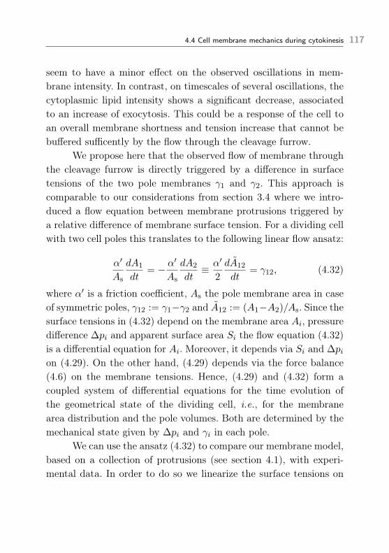
4.4 Cell membrane mechanics during cytokinesis 117
seem to have a minor effect on the observed oscillations in mem-brane intensity. In contrast, on timescales of several oscillations, thecytoplasmic lipid intensity shows a significant decrease, associatedto an increase of exocytosis. This could be a response of the cell toan overall membrane shortness and tension increase that cannot bebuffered sufficently by the flow through the cleavage furrow.
We propose here that the observed flow of membrane throughthe cleavage furrow is directly triggered by a difference in surfacetensions of the two pole membranes γ1 and γ2. This approach iscomparable to our considerations from section 3.4 where we intro-duced a flow equation between membrane protrusions triggered bya relative difference of membrane surface tension. For a dividing cellwith two cell poles this translates to the following linear flow ansatz:
α′
As
dA1
dt= − α
′
As
dA2
dt≡ α′
2
dA12
dt= γ12, (4.32)
where α′ is a friction coefficient, As the pole membrane area in caseof symmetric poles, γ12 := γ1−γ2 and A12 := (A1−A2)/As. Since thesurface tensions in (4.32) depend on the membrane area Ai, pressuredifference ∆pi and apparent surface area Si the flow equation (4.32)is a differential equation for Ai. Moreover, it depends via Si and ∆pion (4.29). On the other hand, (4.29) depends via the force balance(4.6) on the membrane tensions. Hence, (4.29) and (4.32) form acoupled system of differential equations for the time evolution ofthe geometrical state of the dividing cell, i.e., for the membranearea distribution and the pole volumes. Both are determined by themechanical state given by ∆pi and γi in each pole.
We can use the ansatz (4.32) to compare our membrane model,based on a collection of protrusions (see section 4.1), with experi-mental data. In order to do so we linearize the surface tensions on

118 Applications to cell biophysics J. Schneider
the right-hand side of (4.32) around the symmetric pole state:
γ12 ≈ A∂ γ
∂A
∣∣∣∣symA12 + S
∂ γ
∂S
∣∣∣∣symS12 +
∂ γ
∂∆p
∣∣∣∣sym
∆p12, (4.33)
where the derivatives are evaluated at the symmetry values, A12 :=
(A1 − A2)/As, S12 := (S1 − S2)/Ss and the excess area in the formAi := Ωi + 1 ≡ Ai/Si. We expand γ in terms of the excess area,instead of the membrane area A itself, because we think that theamount of membrane in excess drives membrane flow rather thanthe absolute area. Moreover, the analytical expression of γ for sphe-rical caps (see (3.17) on page 75) takes the simplest form for thevariable set A, S and ∆p. The point force f does not enter the ex-pansion (4.33) because we assume that it is, in good approximation,independent of the myosin concentration and thus remains constantin each cell pole. In a next step we replace the occurring pressu-re difference ∆p12 by (4.29) and divide by the prefactor in front ofA12 in (4.33). Hence, the flow equation (4.33) can be written in thelinearized form
A12 = −βSS12 + βAdA12
dt+ βV
dV12
dt(4.34)
with
βS :=S
A
∂Sγ
∂Aγ
∣∣∣∣sym
, βA =α′
2A
1
∂Aγ
∣∣∣∣sym
, βV =α
2A
∂∆pγ
∂Aγ
∣∣∣∣sym
. (4.35)
By assuming that the measured total membrane intensities (Figu-re 4.6b) are proportional to the membrane areas, we can concludethat the quantities normalized by their symmetric values are iden-tical, i.e., Ai = I
(i)mem. Then we can plug into (4.34) the measured
experimental data, namely the apparent pole areas, the pole volu-

4.4 Cell membrane mechanics during cytokinesis 119
mes and the membrane intensities, and apply a multidimensionalleast square fit to obtain the parameters βS , βA and βV . The resultfor the example cell in Figure 4.6b is shown in Figure 4.6c. The ob-tained errors for βA and βV are with 34 % and 46 %, respectively,relatively large. This could be due to the fact that the experimen-tal data does not provide enough oscillations. Also the number ofdata points per oscillation is with nine relatively small. However,we can draw two preliminary conclusions from the fit result. First,we find that the terms related to S12 and A12 in (4.34) cancel eachother in good approximation, meaning that the membrane bucklingis predominantly determined by the change of apparent surface area(section 4.4.1). This is in agreement with the small area flow acrossthe cleavage furrow, discussed above. Hence, (4.34) roughly simplifiesto A12 ∼ V12.
The second conclusion from the fit is related to the result forβS . Since this parameter does not depend on the friction coefficientsα and α′ it can directly be related to our membrane model from sec-tion 4.1. We can numerically evaluate the derivatives of the surfacetension γ(A,S, ∆p, f) (see Figure 3.5 on 75) with respect to S andA and then solve
βS =S
A
∂Sγ
∂Aγ
∣∣∣∣sym⇒ As = As(Ts,Ss, f ,βS)
Ts→∞∝ 2βS − 1
βS − 1(4.36)
for the membrane excess area As in the symmetric pole state. Thedependency of γ on the pressure difference ∆p is replaced by thecortex tension T via the force balance (4.6). The resulting excessarea is plotted as a function of Ts in Figure 4.6d. It increases fromAs ≈ 1 at Ts = 0 to As ≈ 2 for typical tensions in the cell cortex(Ts ∼ 500 pN/µm, see section 1.1.1). In the limit of Ts → ∞ theexcess area converges to As = 2.5, which is the analytical result in(4.36) for a membrane consisting of spherical caps.

120 Applications to cell biophysics J. Schneider
The estimated range for the membrane excess area in the sym-metric case suggests that a large part of the extra membrane neededto cover the expanding cell pole can be provided by this initial ex-cess. We can estimate the value of the minimal excess area requiredfor the observed cell pole deformations from the typical magnitudeof the pole area expansions. This is of the order of 50 % [26]. Sub-tracting 10 % provided by lipid flow through the cleavage furrow,a remaining 40 % must be buffered by unfolding initially buckledmembrane. Hence, we have As & 1.4 which agrees with our estimatein Figure 4.6d.
In future work we want to compare the estimated values forthe membrane excess to a quantitative analysis of membrane out-of-plane structures during cell pole oscillations, observed with electronmicroscopy pictures as shown in Figure 1.6 on page 40. In this con-text we also want to further investigate the role of membrane tubes(microvilli) initiated by cortical filaments (f > 0) which occur du-ring pole oscillations. So far we only included small pushing forces tothe surface tension in (4.36). These are, however, not large enoughto induce such membrane tubes (see section 3.2.4).
4.4.3 | Membrane buckling as a contribution for cell elasticityduring cytokinesis
Via (4.29) the buckling of membrane, which, as we argue, is drivenby cell pole oscillations, could itself feedback onto these oscillations.This is because ∆p12 depends on the lateral membrane tensions γ‖1and γ‖2 as introduced in (4.6). These tensions, in turn, depend on thebuckling state of the membrane and the present pressure difference.In general, ∆p12 can then only be determined implicitly. We derivehere an explicit expression by linearizing γ‖i in a similar way asthe surface tension γi in the previous section. In principle, also γ‖i

4.4 Cell membrane mechanics during cytokinesis 121
contraction expansion
a
0
10
20
0.9 1
γ‖
[pN
/µm
]
lp/lps
f = 0
Ts = 300 100
0
10
20Ts = 300
f = 50∝K2Dlp/lps
b
0
200
400
600
800
1000
0.05 0.1 0.15 0.2
K2D
[pN
/µm
]
Ωs
5f = 0
3Ts
c
Figure 4.7 | Surface elasticity caused by membrane buckling. a illustrates thefolding of the anchored membrane caused by pole contractions and expansions. bshows the lateral tension γ‖ as a function of the anchoring mesh size ξ ≡ l (graysolid lines) for two different cortex tensions Ts (in pN/µm, bottom plot) and twodifferent filament forces f (in pN, top plot). The mesh size is normalized bylps = 2
√Ss/πNp ≈ 0.7µm, where Ss ≈ 750.7µm2 is taken from the cell data used
for Figure 4.6. The membrane area is constant and chosen as As = 1.1 Ss. The reddashed line indicates the linear expansion around lps. c shows the surface elasticityK2D as a function of the initial excess area Ωs = As/Ss for Ts = 300 pN/µm andtwo different forces (pN). The red dashed line indicates condition (4.41). For bothb and c we used the full numerical data from chapter 3. κ = 20KBT , C0 = 0 andf = 0.
depends on the three quantities membrane area Ai, apparent polearea Si and pressure difference ∆pi. However, the dependency on Aiwe ignore here due to the relatively small membrane flow through thecleavage furrow which implies A1 ≈ A2. The pressure difference onlycauses a renormalization of the friction coefficient α in (4.29) so thatthe only dependency we include is that of Si. We express it in terms

122 Applications to cell biophysics J. Schneider
of a change of the mesh size ξi ≡ lpi (Figure 4.7b). Plugging this intothe force balance (4.6) we find for ∆p12 of (4.29) the approximation
∆p12 ≈ 2
[T1 + γ‖sR1
−T2 + γ‖sR2
]+K2D
Rslps
(lp1− lp2
). (4.37)
Here γ‖s is the lateral tension in the symmetric state and
K2D := lp∂γ‖
∂lp
∣∣∣∣sym
(4.38)
plays the role of a surface elasticity due to the buckling of membrane.It is plotted in Figure 4.7c. By relating, in linear order, the changeof the mesh sizes to the change of volumes of the spherical portionswe can rewrite (4.37) to
∆p12 ≈ ∆pLaplace +K3D
Vs(V1 − V2) . (4.39)
With this we can deduce the following constitutive expression forthe bulk elasticity K3D, which originally has been introduced as ageneric cell property in (1.2) on page 27 [26]:
K3D =K2D
3Rs
[1− 4
R2c
l2psNp
][1 + 8
R2c
l2psNp
]Rc→0∝ K2D
3Rs. (4.40)
Qualitatively, this result suggests that the bulk elasticity found forcells during cytokinesis is, at least partly, generated by the surfaceelasticity coming from the buckling of the cell membrane. To estima-te the contribution quantitatively we can compare (4.40) with thecharacteristic value of K3D needed to stabilize cell division. Accor-ding to (1.4) on page 28 this is the case if K3D ≈ Ts/Rs. That is,
4.4 Cell membrane mechanics during cytokinesis 123
with (4.40) the condition
K2D!≈ 3Ts (4.41)
must be satisfied so that the buckling elasticity can have an im-pact on the stabilization of cell division. For reasonable cell para-meters (Figure 4.7c) we find that K2D can, indeed, be of the rightorder of magnitude, if the excess area in the symmetric pole stateis Ωs ≈ 0.005. This is smaller than the excess area we estimated inthe previous section. Thus, a further investigation is needed to verifythe buckling of membrane in the symmetric state of oscillating cells.As pointed out in the previous section, the quantification of electronmicroscopy images will help to clarify this. On top of that, the im-pact of membrane tubes on K2D, which occur for f 1, needs tobe explored further.
However, already the fact that we find the membrane to beable to generate a sufficiently large elastic response under certainconditions is striking as the cell membrane is usually regarded asrelatively flexible (κ = 20 kBT ). The reason for such a strong ela-stic response is the buckling on relatively small length scales of lessthan a micrometer. This shows that membrane buckling is not onlytriggered by the volume change but can, in principle, also feedbackto the volume change. In this spirit, the discussed membrane beha-vior during cytokinesis is a demonstrative example for the coupledmechanics of cell membrane and cortex, introduced by our self-con-sistent description in section 4.2.1.


CONCLUSIONS AND OUTLOOK 5
With the work presented in the last chapters we provide a relativelysimple theoretical description of the interplay between cell membraneand cortex. For the actual anchoring of the membrane to the cortexwe introduced two different approaches. One treated the membra-ne as a relatively flat sheet attached via discrete anchoring pointsto a square lattice. The other treated the membrane as a collecti-on of axisymmetric protrusions also arranged on a square lattice.These approaches allowed us to relate the buckling of the anchoredmembrane to its shape and, via its surface tension, to its mechanicalstate. Interestingly, we found that the description in the weak-ben-ding approximation is neglecting significant terms for the surfacetension of the membrane, indicating that this approximation, oftenused in previous work, could be inappropriate for a mechanical ana-lysis of the membrane. For our work this became important becauseonly with the full description we could predict bleb formation dueto membrane flow, as reported earlier [155]. With this finding and afurther analysis of bleb formation due to a local detachment from thecortex, the analysis of invaginated membrane tubes and the analysisof filament induced extrusion of microvilli we found shape diagramswhich determine the conditions under which these structures shouldoccur in cells.
We used our results for the mechanics of a buckled, anchored
125

126 Conclusions and outlook J. Schneider
membrane to propose a closed system of equations for the interplayof cell membrane and cortex. It enables us to relate subcellular pro-perties of the cell to global cell properties. Most importantly, we canrelate the contractility of the cell cortex, generated by active mo-tor proteins, to the equilibrium radius of the cell, the cell pressuredifference compared to the outside, the membrane surface tensionand to the shape of the anchored membrane. A striking result ofthis new description is that the membrane is buckling, i.e., it is nottightly attached to the cortex, as usually assumed in the past, but isnaturally deformed into small bulges, even in absence of curvaturemodulating proteins. This buckling is induced by the contractility inthe cortex. Moreover, local expansions and contractions of the cor-tex can trigger a redistribution of membrane area among the bulges,leading to a further enhancement of the buckling in the contractedand a depletion in the expanded parts. We studied this phenomenonfor dividing cells that exhibit persistent cell pole oscillations. We de-monstrated how the membrane area redistribution is self-regulatedby the membrane as it equilibrates its surface tension by membraneflow through the cleavage furrow of the dividing cell. Furthermore,we showed that the change of buckling during the redistribution gi-ves rise to an effective elastic response of the membrane, due to thechange of curvature energy, large enough to have a significant impacton the overall cell elasticity. These findings give, on the one hand, anew insight into how mechanics regulate the membrane, in particu-lar, the buffering of fast occurring excess area. On the other hand,they suggest that the membrane not only reacts to other (activelydriven) mechanical processes inside the cell but could itself feedbackmechanically through its buckling state.
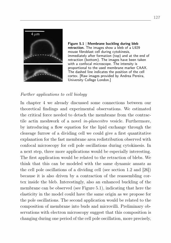
127
Figure 5.1 | Membrane buckling during blebretraction. The images show a bleb of a L929mouse fibroblast cell during cytokinesis,immediately after formation (top) and at the end ofretraction (bottom). The images have been takenwith a confocal microscope. The intensity isproportional to the used membrane marker CAAX.The dashed line indicates the position of the cellcortex. [Raw images provided by Andrea Pereira,University College London.]
Further applications to cell biology
In chapter 4 we already discussed some connections between ourtheoretical findings and experimental observations. We estimatedthe critical force needed to detach the membrane from the contrac-tile actin meshwork of a novel in-planevitro vesicle. Furthermore,by introducing a flow equation for the lipid exchange through thecleavage furrow of a dividing cell we could give a first quantitativeexplanation for the fast membrane area redistribution observed withconfocal microscopy for cell pole oscillations during cytokinesis. Ina next step, three more applications would be especially interesting.The first application would be related to the retraction of blebs. Wethink that this can be modeled with the same dynamic ansatz asthe cell pole oscillations of a dividing cell (see section 1.2 and [26])because it is also driven by a contraction of the reassembling cor-tex inside the bleb. Interestingly, also an enhanced buckling of themembrane can be observed (see Figure 5.1), indicating that here theelasticity in the model could have the same origin as we propose forthe pole oscillations. The second application would be related to thecomposition of membrane into buds and microvilli. Preliminary ob-servations with electron microscopy suggest that this composition ischanging during one period of the cell pole oscillation, more precisely,

128 Conclusions and outlook J. Schneider
Figure 5.2 | Experimentally measured membrane protrusions fitted by theoreticalshapes. Overlaid are the experimental contour lines (blue) and the contourobtained by a theoretical fit (red) on top of images taken by an electronmicroscope. Same cell type as in Figure 5.1. [Raw images provided by OrtrudWartlick, University College London.]
the fraction of tubes covering the cell is varying. We should be able,in principle, to localize the position of these cells within our sha-pe diagrams and, thus, explain this variation. A third application,which we recently started to explore, uses single protrusion images(Figure 5.2), also obtained from electron microscopy, to fit their con-tour line by the contour of our theoretical shapes from section 3.21.As we fix the bending rigidity (κ = 20 kBT ), we can estimate thesurface area Ap of the protrusion and the pressure difference ∆p fromthe fit. Therewith, we can calculate the surface tension γ and thelateral tension γ‖ of the membrane. The results could be compared,for instance, with separate measurements of ∆p and γ.
Possible extensions of the presented concepts
In order to perform more quantitative comparisons with experimen-tal observations it might be necessary to further extend our theore-tical concepts and thus make the modeling more realistic. We think
1 Similar studies have been reported recently for endosome formation [206].

129
Figure 5.3 | Membrane sheet bound toa hexagonal lattice. The dashed circlesillustrate the basal area of membraneprotrusions, here with differentdiameters.
for future work especially two such extensions would be important,namely to consider integral membrane proteins and a heterogeneousanchoring mesh. The latter could be implemented by keeping theintroduced square lattice at fixed mesh size ξ but to allow eachprotrusion to have a different basal diameter lpnm , as illustrated inFigure 5.3. As a consequence of this heterogeneity, in equilibrium,each protrusion would carry a different excess area what could giverise to new interesting shape states. Similarly, also integral prote-ins could modify the distribution of excess area. Reason for this istheir prohibited diffusion across the anchoring sites, in contrast tolipid diffusion. This would lead to unbalanced protein concentrati-ons among protrusions and could induce an entropic tension thatmodifies the actual surface tension.
On top of this, a few further extensions could be considered forour work. For example, protrusions without axial symmetry couldbe included. To account for the spherical geometry of the cell, theirboundary condition at the base could be changed as (compare toconditions (3.2) on page 63)
ψ(0) = 0 → ψ(0) = arcsinl
2R. (5.1)

130 Conclusions and outlook J. Schneider
Furthermore, instead of a square lattice, a hexagonal lattice, as illu-strated in Figure 5.3, would fit more accurately to an axisymmetricprotrusion. Finally, in addition to the flow equation, the effect ofendocytosis and exocytosis for the membrane description during cellpole oscillations could be included by separate equations, modelingthe lipid exchange between membrane and cytoplasm.
A very interesting theoretical aspect, which we faced throug-hout our work, however, did not study any further until now, is tounderstand the underlying mechanisms for the formation and per-sistence of the anchoring lattice. We argued along the line of thefences model, introduced in the past [59, 66], i.e., that the charac-teristic mesh size is determined by the meshwork size of the cellcortex. However, this remains a hypothesis. An experimental analy-sis of this would be interesting. Another approach, which could leadto a different mesh size than the one purely dictated by the cortex,would involve a minimization of the membrane energy F also withrespect to the linker diameter. According to its definition (3.19) onpage 76, the lateral tension is always zero then and the minimizationreturns an additional relation (see derivation of the shape equationsin appendix B.3)
δρ(0) 6= 0 ⇒ l = l(A, ∆p, f). (5.2)
Independently of how the lattice size is determined, in either caseanother important question is how it is maintained. This question isrelevant because on long enough timescales the viscous properties ofthe cortex dominate (see section 1.1.1), suggesting that then mem-brane anchors can slide in lateral direction. The consecutive questionis whether a homogeneous structuring of the membrane into protru-sion can then be stable at all. This can be checked in the same wayas the stability of a homogeneous area distribution. Following thederivation of (3.29) on page 84, the stability of the anchoring lattice

131
is defined by the derivative2
∂γ‖
∂l> 0 ⇒ stable homogeneous lattice. (5.3)
Otherwise a small perturbation would lead to a contineous growth ofone protrusion base until, eventually, the entire membrane is mostlydetached from the cortex. As Figure 4.7b on page 121 shows, accor-ding to our membrane model a positive slope of γ‖(l) is possible,indicating that the protrusion structure is stable even on timescaleswhere the cortex becomes viscous.
2 Note that here the sign is the opposite to the sign for the membrane flow becausea locally larger lateral tension tends to reduce the respective protrusion diameter.


APPENDIX
DIFFERENTIAL GEOMETRY OF SURFACES A
Differential geometry is the mathematical framework which descri-bes the geometrical shape of any n-dimensional object [210]. It isused for coordinate transformations between different coordinate sy-stems suitable for different geometries, mostly in the context of cur-ved spaces or surfaces.
The main concepts of differential geometry can be seen as ageneralization of what is known from linear algebra and vector ana-lysis. An arbitrary vector a can be expressed by basis vectors gias [210]1:
a = ai gi, (A.1)
where ai are the components of a. Here the components and basisvectors are defined locally, i.e., they depend on the spatial position.Furthermore, the basis vectors are in general not normalized andnot orthogonal. In cartesian coordinates, where gi is equal to thecartesian unit vector ei, they form a constant orthonormal basis.The scalar product of two vectors a and b
a · b = aibjgi · gj ≡ aibjgij (A.2)
1 Here Einstein’s summation convention∑i aib
i ≡ aibi is used.
133

134 Differential geometry of surfaces J. Schneider
Figure A.1 | Schematic of aparameterized curved surface. bu
and bv are the tangential vectors, nthe normal vector. ei are thecartesian unit vectors.
defines the metric or metric tensor gij . It determines the geometry,i.e., the distances and angles in the coordinate space. The metric issymmetric and becomes diagonal for orthogonal coordinate systems.For the cartesian coordinate system gij is equal to the Kroneckersymbol δij . Either the metric or the scalar product itself are alsocalled the first fundamental form of differential geometry.
Often the first fundamental form is defined via the squaredline element
ds2 ≡ dr · dr = gijdxidxj . (A.3)
It provides a relatively simple way to compute the transformationbehavior of the metric under a change of coordinates since any infini-tesimal coordinate displacement can be expressed in new coordinateswith the help of the total differential. It follows:
ds2 = gijdxidxj = gij
∂xi
∂x′n∂xj
∂x′mdx′ndx′m ≡ g′nmdx′ndx′m, (A.4)
where the prime denotes the new coordinates. According to (A.4)the basis transformation reads
g′i =∂xi
∂x′jgj . (A.5)
The basis vectors tangential to the coordinate lines are then defined
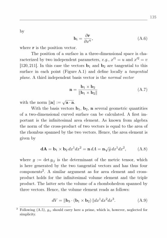
135
by
bi =∂r
∂x′i, (A.6)
where r is the position vector.The position of a surface in a three-dimensional space is cha-
racterized by two independent parameters, e.g., x′1 = u and x′2 = v
[120, 211]. In this case the vectors b1 and b2 are tangential to thissurface in each point (Figure A.1) and define locally a tangentialplane. A third independent basis vector is the normal vector
n =b1 × b2
‖b1 × b2‖(A.7)
with the norm ‖a‖ :=√a · a.
With the basis vectors b1, b2, n several geometric quantitiesof a two-dimensional curved surface can be calculated. A first im-portant is the infinitesimal area element. As known from algebrathe norm of the cross-product of two vectors is equal to the area ofthe rhombus spanned by the two vectors. Hence, the area element isgiven by
dA = b1 × b2 dx1dx2 = n dA = n
√g dx1dx2, (A.8)
where g := det gij is the determinant of the metric tensor, whichis here generated by the two tangential vectors and has thus fourcomponents2. A similar argument as for area element and cross-product holds for the infinitesimal volume element and the tripleproduct. The latter sets the volume of a rhombohedron spanned bythree vectors. Hence, the volume element reads as follows:
dV = ‖b3 · (b1 × b2) ‖dx1dx2dx3. (A.9)
2 Following (A.5), gij should carry here a prime, which is, however, neglected forsimplicity.

136 Differential geometry of surfaces J. Schneider
A third important geometrical quantity is the curvature of the sur-face. It can be defined as the second spatial derivative of the positionvector r. In two dimensions this is summarized in the curvature ten-sor
Cij = −n · g′ik ∂
∂x′j∂
∂x′kr , (A.10)
where g′ik is the dual or conjugate metric to g′ik. Both are coupled toeach other via the relation g′ing
′nk = δki . That is, g′ik is the inverseof g′ik.
The curvature tensor (A.10) can also be interpreted as a mea-sure for how much the tangential plane in a certain point is changingits orientation in a small vicinity. Therefore, the curvature tensor gi-ves rise to two principal axes on the surface, which correspond to thetwo invariant scalar principal curvatures C1 and C2. A more naturalchoice for such a pair of curvature invariants is given by the meancurvature H and Gaussian curvature K, because they can direct-ly be extracted from Cij by its trace 2H = trCij and determinantK = detCij , respectively. Due to this and the fact that Cij is sym-metric, each pair can be calculated by the other via the relationsH = (C1 + C2)/2 and K = C1C2.

APPENDIX
VARIATIONAL PRINCIPLEAND THE SHAPE EQUATIONS B
B.1 | Variation calculus
With the calculus of variation extrema of functionals, which dependon variables that themselves depend on space or time, can be cal-culated. The variation of the functional G, which depends on thefunction f(ξ), where ξ is a not further specified set of variables, isdefined as [140,212]
δG[f ] := limδf→0
G[f + δf ]−G[f ] . (B.1)
The functional is the equivalent to the differential or more preciselythe total differential of a function, depending on a number of varia-bles [212]. It can be shown that the functional obeys a generalizedrelation of the total differential
δG[f ] =
∫dξδG
δfδf (B.2)
or if G depends on several functions as
δG[f1, f2, . . . ] =
∫dξ
δG
δf1δf1 +
δG
δf2δf2 + . . .
. (B.3)
137

138 Variational principle and the shape equations J. Schneider
Relations (B.2) and (B.3) act as a definition for the functional de-rivative δG/δf . As in basic analysis the vanishing of the functionalderivative is a necessary condition for finding extrema. However, he-re the extrema are functions instead of single parameters. That iswhy the functional derivative leads, in principle, to a differentialequation, from which the extremal function can be determined.
If the function G appears in the form
G[f1, f2, . . . ] =
∫dξ L[f1, f2, . . . ]. (B.4)
the variation of G leads directly to a variation of the integrant L,which can be expanded up to linear order in δf1, δf2, . . . . If G alsodepends on derivatives of f1, f2, . . . , a partial integration is necessaryin order to bring the variation in the form (B.4). The occurring boun-dary terms have to vanish identically. This is either automaticallyguaranteed by existing boundary conditions or leads to additionalboundary conditions. The resulting expressions for the functionalderivatives are called Euler-Lagrange equations as they are set tozero.
In the following the variational principle is used to calculatethe shape equations for a membrane, described by the energy (seealso (1.6) on page 30)
F =κ
2
∮dA(2H − C0)2 + γΞ−∆p
∫dV − f
∫dL (B.5)
with
Ξ :=
∮dA γ = const.,∮dA−A A = const.
(B.6)
Two special parameterizations are used for the variation, the Mongeparameterization and the arc length parameterization. For the first,the force term in (B.5) will be neglected (f = 0).

B.2 Shape equations in Monge parameterization 139
B.2 | Shape equations in Monge parameterization
The Monge parameterization describes the position of a two-dimen-sional surface by a height function h with respect to a referenceplane. The two special cases, used in this work, are the cartesianreference frame (h(x, y)) and a cylindrical reference plane (h(ρ,ϕ)).A schematic illustration can be found in Figure 1.5a on page 35.
Monge parameterization h(x, y)
In order to derive the shape equations expressed by h(x, y), first, thearea element dA, the volume element dV and the mean curvatureH in the energy (B.5) need to be rewritten explicitly. An overviewof their explicit expressions is given in Table B.1 at the end of thissection. The energy can then be written as1
F =
∫dx dyL(h,h|x,h|y,h|xy,h|xx,h|yy) (B.7)
with
L =−∆p h+ γ√g
+κ
2
√g
(2h|xh|yh|xy − h|xxg(y) − h|yyg(x)
√g3 − C0
)2
.(B.8)
The used notation h|x := ∂h∂x is used for simplicity. From (B.7) the
variation δF (B.1) yields
δF =
∫dxdy
[∂L∂h
δh+∂L∂h|x
δh|x +∂L∂h|y
δh|y
+∂L∂h|xy
δh|xy +∂L∂h|xx
δh|xx +∂L∂h|yy
δh|yy
].
(B.9)
1 Here and in the following the constant energy term −γA, which might occuraccording to (B.5) for a constant surface area, is skipped.

140 Variational principle and the shape equations J. Schneider
By interchanging the partial with the functional derivative, δh|x =
∂xδh, (B.9) can be rewritten with the help of partial integrations insuch a way that all bulk terms contain the variation δh:
δF =
∫dx dy
[∂L∂h− ∂
∂x
∂L∂h|x
− ∂
∂y
∂L∂h|y
+∂2
∂x∂y
∂2L∂h|xy
+∂2
∂x2
∂2L∂h|xx
+∂2
∂y2
∂2L∂h|yy
]δh
+
∫dx
[∂L∂h|y
− ∂
∂y
∂L∂h|yy
− ∂
∂y
∂L∂h|xy
]δh
∣∣∣∣y2
y1
+
∫dy
[∂L∂h|x
− ∂
∂x
∂L∂h|xx
− ∂
∂x
∂L∂h|xy
]δh
∣∣∣∣x2
x1
+
∫dx
[∂L∂h|yy
]δh|y
∣∣∣∣y2
y1
+
∫dy
[∂L∂h|xx
]δh|x
∣∣∣∣x2
x1
+∂L
∂h|xyδh
∣∣∣∣x1,y1
+∂L
∂h|xyδh
∣∣∣∣x2,y2
− ∂L∂h|xyδh
∣∣∣∣x1,y2
− ∂L∂h|xyδh
∣∣∣∣x2,y1
.
(B.10)
The boundary terms in the Monge parameterization can often im-mediately be neglected due to periodic boundary conditions. In thiscase the values of h(x, y) and its derivatives will be equal at theboundaries x = x1 and x = x2 and y = y1 and y = y2, respectively.The integrand L will then also take the same values there and theboundary terms cancel each other. The bulk term in (B.10) leadsfor δF !
= 0 to the Euler-Lagrange equation for the specific problem(B.7). The full evaluation for the given L in (B.10) leads to a re-latively complicated nonlinear partial differential equation for theequilibrium shape. A simpler expression of the shape equation can

B.2 Shape equations in Monge parameterization 141
be obtained with the help of the weak-bending approximation, where∂h/∂x ≈ ∂h/∂y ≈ 0. A more detailed explanation is provided inparagraph 1.3.3 on page 34. With this approximation the integrand(B.8) can be expanded up to the first nontrivial order:
L ≈ (γ +κ
2C2
0 −∆p h) + C0κ(h|xx + h|yy
)+κ
2
(h2|xx + h2
|yy + 2h|xxh|yy
)+
1
2
(γ +
κ
2C2
0
)(h2|x + h2
|y
).
(B.11)
Computing the bulk term of (B.10) based on (B.11) leads to theshape equation in weak bending approximation:
42‖h(x, y)− γ∗
κ4‖h(x, y) =
∆p
κ(B.12)
withγ∗ := γ +
κ
2C2
0 . (B.13)
Monge parameterization h(ρ)
In general, an equivalent choice for the height function h(x, y) isthe height function h(ρ,ϕ) with the cylindrical coordinates ρ andϕ. Especially for disc-like membrane sheets it has advantages com-pared to the cartesian Monge parameterization. This becomes mostobvious for the special case where this disc has axial symmetry. Thenthe cylindrical Monge parameterization simplifies to an effective one-dimensional problem described by h(ρ).
Also for the axisymmetric case with h(ρ) the geometrical quan-tities are summarized in Table B.1 at the end of this section. The
142 Variational principle and the shape equations J. Schneider
energy (B.5) then reads as
F = 2π
∫dρL(ρ;h,h|ρ,h|ρρ) (B.14)
with
L =−∆p ρ h+ γρ√g
+κ
2ρ√g
(ρh|ρρ + h3
|ρ + h|ρ
ρ√g3 + C0
)2
.(B.15)
The variation follows as
δF = 2π
∫dρ
[∂L∂h− d
dρ
∂L∂h|ρ
+d2
dρ2
∂L∂h|ρρ
]δh
+∂L∂h|ρ
δh
∣∣∣∣ρ2
ρ1
+∂L∂h|ρρ
δh|ρ
∣∣∣∣ρ2
ρ1
− d
dρ
∂L∂h|ρρ
δh
∣∣∣∣ρ2
ρ1
.
(B.16)
For this work the boundary terms are negligible due to the imposedboundary conditions imposed. The shape equation, obtained fromthe bulk term, reads as
f(1)h + γ f
(2)h = 0 (B.17)
with
f(1)h =
κ
2ρ2√g9
[h|ρ(1− ρ2C2
0
)g4
+(h|ρ + ρh|ρρ − ρ3C2
0h|ρρ)g3
+ρ(−3h|ρρ + 4ρh|ρρρ + 2ρ2h|ρρρρ
)g2
−4ρ2C0h|ρh|ρρ√g5
+ 5ρ2h|ρρ
(6ρh2
|ρρ − 3h|ρh|ρρ − 4ρh|ρh|ρρρ
)g
B.3 Shape equations in arc length parameterization 143
−35ρ3h3|ρρ
]−∆pρ,
f(2)h =−
(g h|ρ + ρ h|ρρ
)√g3 . (B.18)
Also here the weak-bending approximation dh/dρ ≈ 0 can be usedto linearize the shape equations. The integrand (B.15) becomes then
L ≈ ρ2
(C2
0κ+ κhρρ(2C0 + h|ρρ
)+ 2γ
)−∆p ρ h
+h2|ρ
4ρ
(C2
0κρ2 + 2κ+ 2ρ2γ
)+ κhρ
(C0 + h|ρρ
) (B.19)
and, thus, the shape equation
κ
(1
ρ2− γ
κ
)h|ρ − κρ
(1
ρ2+γ
κ
)h|ρρ
+ 2κh|ρρρ + κρh|ρρρρ = ∆pρ.
(B.20)
B.3 | Shape equations in arc length parameterization
The Monge parameterization h(ρ), discussed in the previous section,cannot be used for surfaces with height gradients above an angle ofπ/2 as then uniqueness of the height function is violated. In thesecases the arc length parameterization can be used instead. It allowsfor arbitrary height gradients and can for axial symmetry. The usedparameters are the arc length s along the contour line of the surface(see Figure 1.5b on 35) and the polar angle ϕ. The correspondingcoordinate transformation for axisymmetric surfaces and the resul-ting geometrical quantities are listed in Table B.1 at the end of thissection. They yet contain two shape functions ρ(s) and h(s). Theycan be replaced by a single shape function ψ(s) via the following

144 Variational principle and the shape equations J. Schneider
relations:∂ρ
∂s= − cosψ,
∂h
∂s= sinψ. (B.21)
ψ(s) is the tilt angle between the tangent of the contour line andthe ρ-axis. Due to these two relations, as discussed in section 1.3.3,the energy (B.5) needs to be extended by two Lagrange terms inorder to ensure that the relations are conserved while the variationis performed. Thus the energy reads as
F∗ = F + µ(s)
(∂ρ
∂s+ cosψ
)+ ν(s)
(∂h
∂s− sinψ
)(B.22)
with µ(s) and ν(s) being two Lagrange multiplier. Using the angle ψchanges the area element, volume element and mean curvature fromTable B.1 in the following way:
dA = ρ dϕds,
dV = ρ dϕdρ ds sinψ,
H =1
2
(sinψ
ρ− ψ|s
). (B.23)
The energy (B.22) then deduces to
F∗ = 2π
∫dsL(ψ,ψ|s, ρ, ρ|s,h,h|s,µ, ν) (B.24)
with
L =1
2κρ
(sinψ
ρ− ψ|s − C0
)2
− 1
2∆p ρ2 sinψ + γρ
+ µ(ρ|s + cosψ
)+ ν
(h|s − sinψ
)− f
2πsinψ.
(B.25)
Here a new term, compared to the two integrands (B.8) and (B.15)from the previous sections, appears, associated with the point force

B.3 Shape equations in arc length parameterization 145
f . It arises from the term fL of the energy (B.5) which was notconsidered before. L is the elevation of the membrane above a fixedground at the position where the perpendicular point force f is app-lied. For axisymmetric membranes the direction of this point force iscollinear to the z-axis of the coordinate system and from the secondrelation of (B.21) the elevation can be deduced to
L ≡ h(s2)− h(s1) =
∫ s2
s1
ds sinψ. (B.26)
The contour length Λ of the contour line, which is paramete-rized by the arc length, is in general not fixed. Therefore, it mustbe part of the variation δF∗. One way to realize this, as reportedin [148], is to directly include the integral boundaries s1 and s2 tothe variation. An equivalent realization, used here, uses a normali-zed arc length u, normalized by the contour length as u := 2s/Λ. Iffurthermore the integral boundaries are chosen such that s1 = 0 thefollowing transformation rules apply:∫ Λ
2
0ds→
∫ 1
0
Λ
2du,
d
ds→ 2
Λ
d
du, L → L∗ =
Λ
2L. (B.27)
As Λ does not depend on u the variation of F∗ with respect to Λ issimply given by the derivative
∂F∗
∂Λ= 2π
∫ 1
0du∂L∗
∂Λ. (B.28)
The variation of F∗ is then given by
δF∗ = 2π
∫ 1
0du
[∂L∗
∂ψ− d
du
∂L∗
∂ψ|u
δψ +
∂L∗
∂ρ− d
du
∂L∗
∂ρ|u
δρ
+
∂L∗
∂h− d
du
∂L∗
∂h|u
δh+
∂L∗
∂ηδη +
∂L∗
∂νδν + 2
∂L∗
∂Λ
]

146 Variational principle and the shape equations J. Schneider
+∂L∗
∂ψ|uδψ
∣∣∣∣10
+∂L∗
∂ρ|sδρ
∣∣∣∣10
+∂L∗
∂h|sδh
∣∣∣∣10
. (B.29)
Evaluating the bulk terms of (B.29) leads to the following set ofshape equations:
0 =−∆pΛρ2 cosψ − 8κ
Λρψ|uu + κΛ
sin 2ψ
ρ
+1
π
(4πκψ|u − fΛ− 2Λπν
)cosψ − 2Λµ sinψ, (B.30)
0 = 2 γΛ + C20κΛ + 4C0κψ|u − 2∆pΛρ sinψ
− κΛsin2 ψ
ρ2+
4κ
Λψ2|u − 4µ|u, (B.31)
0 = ν|u, (B.32)
0 =Λ
2cosψ + ρ|u, (B.33)
0 = − Λ
2sinψ + h|u, (B.34)
0 = 2π
∫ 1
0du
[ρ
(2γ + C2
0κ−4κ
Λ2ψ2|u
)−2C0κ sinψ − f
πsinψ −∆pρ2 sinψ
+κsin2 ψ
ρ+ 2µ cosψ − 2ν sinψ
]. (B.35)
Note that the integrand of the last equation, or equivalently of(B.28), has a special meaning, as pointed out in [148]. It can beshown that
2∂L∗
∂Λ≡ −H∗ (B.36)
with the Hamilton function
H∗ = −L∗ + ψ|u∂L∗
∂ψ|u+ ρ|u
∂L∗
∂ρ|u+ h|u
∂L∗
∂h|u. (B.37)

B.3 Shape equations in arc length parameterization 147
Arc length parameterization for smooth boundary conditions
In this work the arc length parameterization is used to describe axi-symmetric membrane protrusions as shown in Figure 3.1 on page62. They have a fixed basal diameter l and are subject to smoothboundary conditions which read according to (3.2) on page 63 as
h(u = 0) = 0, ρ(u = 0) = l/2, ρ(u = 1) = 0,
ψ(u = 0) = ψ(u = 1) = 0. (B.38)
From this the boundary terms in (B.29) (or rewritten for u as in(1.24) on page 38) can be evaluated immediately. The variations δψand δρ vanish at both ends and, hence, the boundary terms as well.However, δh only vanishes for u = 0. This gives rise to an additionalboundary condition for ν:
∂L∗
∂h|u
∣∣∣∣u=1
= ν(u = 1) = 0. (B.39)
With this and (B.38) there are six conditions for six integrationconstants, arising from the integration of the shape equations (B.30)– (B.35).
Having the boundary conditions (B.38) and (B.39), three sha-pe equations can be solved immediately. From (B.32) ν deduces to
ν(s) = 0. (B.40)
With the help of (B.33) and (B.34), which are equivalent to theimposed relations (B.21), expressions for ρ and h can be found:
ρ(u) =l
2− Λ
2
∫ u
0du′ cosψ(u′), (B.41)
h(u) =Λ
2
∫ u
0du′ sinψ(u′). (B.42)

148 Variational principle and the shape equations J. Schneider
The remaining three shape equations need to be solved simultaneous-ly, in principle, as they are coupled with each other. This requiresthe help of numerical methods as they are not solvable analytically.The method, used in this work, is discussed in appendix D. For thismethod it is convenient to reformulate these three equations. Firstly,(B.33) can be integrated once and then be written as
µ(u) = γΛ
2u+ µint(u) + µ0 (B.43)
with
µint(u) :=1
4
∫ u
0du′[C0κ
(4ψ|u′ + ΛC0
)− 2∆pΛρ sinψ
−κΛsin2 ψ
ρ2+
4κ
Λψ2|u′
] (B.44)
and µ0 being an integration constant. This constant is set by thesecond boundary condition for the radius ρ(1) = 0. With the help of(B.41) this can be translated to the condition
l = Λ
∫ 1
0du cosψ. (B.45)
Finally, with (B.43) µ can be replaced in the two other equations(B.30) and (B.35), which then become
0 =f(1)ψ + γf
(2)ψ + µ0f
(3)ψ , (B.46)
0 =f(1)Λ + γf
(2)Λ + µ0f
(3)Λ (B.47)
with
f(1)ψ =
(4πκψ|u − fΛ
)π
cosψ −∆pΛρ2 cosψ

B.3 Shape equations in arc length parameterization 149
− 8κ
Λρψ|uu + κΛ
sin 2ψ
ρ− 2Λµint sinψ,
f(2)ψ =− Λ2u sinψ,
f(3)ψ =− 2Λ sinψ,
f(1)Λ =
1
2
∫ 1
0du
[C2
0κρ−(2πC0κ+ f)
πsinψ −∆pρ2 sinψ
−4κ
Λ2ρψ2|u + κ
sin2 ψ
ρ+ 2µint cosψ
],
f(2)Λ =
∫ 1
0du
[ρ+
Λ
2u cosψ
],
f(3)Λ =
∫ 1
0du cosψ. (B.48)
Solving (B.41), (B.46) and (B.47) simultaneously under the conditi-on (B.45) gives the equilibrium shape of an axisymmetric membra-ne area with smooth boundary conditions, described by the energy(B.5). Note that f (1)
ψ , f (2)ψ and f (3)
ψ are still functions of u whereas
f(1)Λ , f (2)
Λ and f (3)Λ are independent of u due to the integration. Also
note that here the surface tension γ is treated as an independentparameter. In section 3.1 and elsewhere in this work γ is determinedby an additional constraint besides (B.45), arising from an imposedsurface area A:
const. ≡ A = πΛ
∫ 1
0du ρ . (B.49)

150 Variational principle and the shape equations J. Schneider
Table B.1 | Geometrical quantities expressed in special parameterizations.Thecoordinate order for the curvature tensor follows the order of appearance of thetangential vectors.
Cartesian Monge parameterization
coordinate transformationx = u, y = v, z = h(u, v) ≡ h(x, y)
basis vectors
bx =
1
0
h|x
, by =
0
1
h|y
, n = 1√g
−h|x−h|y1
area element
dA =√g dx dy with g = 1 + h2
|x + h2|y
volume elementdV = h dx dy
curvature tensor
Cij = − 1√g3
((g − h2
|x)h|xx − h|xh|yh|xy (g − h2|y)h|xy − h|xh|yh|xx
(g − h2|x)h|xy − h|xh|yh|yy (g − h2
|y)h|yy − h|xh|yh|xy
)mean curvature
H = 12√g3
(2h|x h|y h|xy − h|xx (g − h2
|x)− h|yy (g − h2|y))
Cylindrical Monge parameterization with axisymmetry
coordinate transformationx = ρ cosϕ, y = ρ sinϕ, z = h(ρ)
basis vectors
bρ =
cosϕ
sinϕ
h|ρ
, bϕ =
−ρ sinϕ
ρ cosϕ
0
, n = 1√g
− cosϕh|ρ− sinϕh|ρ
1

B.3 Shape equations in arc length parameterization 151
area elementdA =
√g dϕ dρ with g = ρ2(1 + h2
|ρ)
volume elementdV = ρ dϕdρ dh
curvature tensor
Cij = − 1√g3
(ρ3 h|ρρ 0
0 g h|ρ
)mean curvature
H = 12√g3
(g h|ρ + ρ h|ρρ
)Arc length parameterization with axisymmetry
coordinate transformationx = ρ(s) cosϕ, y = ρ(s) sinϕ, z = h(s), h2
|s + ρ2|s = 1
basis vectors
bϕ =
−ρ sinϕ
ρ cosϕ
0
, bs =
ρ|s cosϕ
ρ|s sinϕ
h|s
, n =
h|s cosϕ
h|s sinϕ
−ρ|s
area element
dA = ρ dϕds
volume elementdV = ρ dϕdρ ds h|s
curvature tensor
Cij =
(ρ−1h|s 0
0 ρ|sh|ss − ρ|ssh|s
)mean curvature
H = 12ρ
(ρρ|sh|ss + h|s
(−ρρ|ss + 1
))


APPENDIX
DERIVATION OF THE ANCHOREDMEMBRANE SHEET SOLUTION C
A special solution of the differential equation
Lh = Q, (C.1)
where L is a differential operator and Q a inhomogeneity, can becomputed from the associated fundamental solution1. This funda-mental solution solves the reduced equation [182,183]
Lhf = δ, (C.2)
where δ is Dirac’s delta distribution. The solution h is then given bythe convolution of hf with Q.
The fundamental solution can be computed with the help ofthe Fourier transformation. Applying it to (C.2) leads to an algebraicequation if the coefficients of L are constant. This equation can bethen be solved for the unknown fundamental solution, which is finallyobtained after evaluating the inverse Fourier transformation.
Let now L be the differential operator found in the shape equa-
1 Often the fundamental solution is also called Green’s function.
153

154 Derivation of the anchored membrane sheet solution J. Schneider
tion of appendix B.2 on weakly undulated membrane sheets2:
L = 4‖2 − γ∗4‖ (C.3)
and h the height profile of the sheet3. Furthermore, the two-dimen-sional Fourier transformation shall be defined in this work in thefollowing way:
h(x, y) =1
2π
∫d2k h(kx, ky) e
ik·r, (C.4)
h(kx, ky) =1
2π
∫d2r h(x, y) e−ik·r. (C.5)
The corresponding fundamental solution can then be written as
hf(x, y) =1
(2π)2
∫d2k
eik·r
k4
+ γ∗k2 , (C.6)
where k ≡ ‖k‖ is the absolute value of the wave number vector.In many cases integrals of this type can be evaluated with the helpof the residue theorem. However, for this work this is not explicitlynecessary. Instead the full solution, given by convolution
h(x, y) = (Q ∗ hf)(x, y) (C.7)
≡∫d2r′Q(x′, y′)hf(x− x′, y − y′), (C.8)
is rewritten with the help of (C.6) to
h(x, y) =1
2π
∫d2k
Q(kx, ky)
k4
+ γ∗k2 e
ik·r. (C.9)
2 See also (B.12) for comparison.3 We use in this section the normalizations as introduced in section 3.1: ∆p :=
ξ3
κ∆p, f := ξ
κf C0 := ξ C0, γ∗ := ξ2
κγ∗, F := F/κ.

155
This relation states that the Fourier transform of h(x, y) is equivalentto
h(kx, ky) ≡Q(kx, ky)
k4
+ γ∗k2 . (C.10)
The result (C.10) can now be used to compute h(x, y) for the specialinhomogeneity introduced in section 2.1 for a periodically anchoredmembrane (see (2.5) on page 48):
Q(x, y) = ∆p+
2q∑s=0
f(s)a
∑n,m
Gmn;s (C.11)
with Gmn;s as in (2.2) on page 47:
Gmn;s = δ(x− n− xs)δ(y −m− ys). (C.12)
According to our definitions (C.4) and (C.5), the Fourier transfor-mation of Q reads then as
Q(kx, ky) = 2π
[2q∑s=0
f(s)a e−ik·rs
∑n,m
δ(kx − 2πn)δ(ky − 2πm)
+∆p δ(kx)δ(ky)
]. (C.13)
Evaluating the inverse transformation of (C.10) is then straight for-ward as every term contains a δ-distribution, which allows a directevaluation of the Fourier integral. The only careful treatment is re-quired for the δ-distribution at zeroth mode kx = ky = 0 as thiswould, in principle, lead to a divergent integral. However, here therelevant terms can be suppressed by ensuring the following condition:

156 Derivation of the anchored membrane sheet solution J. Schneider
∆p+
2q∑s=0
f(s)a
!= 0. (C.14)
A physical interpretation of this relation is given in section 2.2.If (C.14) is guaranteed, the Fourier transformation (C.4) of h
can be evaluated:
h(x, y) =
2q∑s=0
f(s)a
∫d2k
eik·(r−rs)
k4
+ γ∗k2
·∑n,m
n=m 6=0
δ(kx − 2πn)δ(ky − 2πm)
=1
16κπ4
2q∑s=0
f(s)a
∑n,m
n=m 6=0
ei2πn(x−xs)ei2πm(y−ys)
(n2 +m2)2 + γ∗
4π2 (n2 +m2)
=
2q∑s=0
f(s)a Γγ∗(x− xs, y − ys) (C.15)
with
Γα(x, y) :=1
4π4
∑n,m≥1
cos (2πnx) cos (2πmy)
(n2 +m2)2 + α4π2 (n2 +m2)
+1
8π4
∑n≥1
cos (2πnx) + cos (2πny)
n4 + α4π2n2
.
(C.16)
The remaining unknowns of (C.15) are the coefficients f (s)a ,
which have been introduced as resistive forces in section 2.1. In to-tal there are 2q + 1 unknown coefficients. So equally many definingequations are needed to fully determine h(x, y). One of these condi-tions is the introduced relation (C.14). The others can be deducedby the fact that all anchoring points shall be localized at the same

157
height. Hence, another 2q equations are defined by
h(x0, y0)!
= h(x1, y1)!
= . . .!
= h(x2q+1, y2q+1) . (C.17)
Together with (C.14), equations (C.17) can be summarized into thefollowing system of equations:
∆p =
2q∑0
f(s)a ,
0 =
2q∑0
[Γγ∗(x1 − xs, y1 − ys)− Γγ∗(x0 − xs, y0 − ys)
]f
(s)a ,
...
0 =
2q∑0
[Γγ∗(x2q − xs, y2q − ys)− Γγ∗(x0 − xs, y0 − ys)
]f
(s)a .
(C.18)
This can also be written in matrix form:
2q∑s=0
M lsf(s)a = N l, (C.19)
where M is a square matrix with the entries
M ls =
1 for l = 0,
Γγ∗(xl − xs, yl − ys)− Γγ∗(x0 − xs, y0 − ys)
otherwise(C.20)
and N a vector with the entries:
N l =
−∆p for l = 0,
0 otherwise.(C.21)

158 Derivation of the anchored membrane sheet solution J. Schneider
The system of equations (C.18) is solved as soon as the inverse matrixM−1 is found. This appears to be not manageable here as long as
the number of anchors is unspecific. The anchor number needs to beset first.
What can be concluded from (C.18) is the explicit dependencyof the coefficients f (s)
a on ∆p. This can be found by only taking asubsystem of (C.18), excluding the first equation. This subsystemis not complete as it consists of 2q equations for 2q + 1 unknowns.Nevertheless, since (C.18) is a linear system, 2q coefficients can beexpressed by the one, which remains undetermined, e.g., f0. In factthey are all proportional to f0, i.e., f1, . . . , f2q ∼ f0. Plugging thisinto the excluded first equation of (C.18) shows immediately that∆p is a linear prefactor of f0 and, hence, for all f (s)
a . However, thisdoes not mean that f (s)
a ∼ ∆p as f (s)a also depends on γ∗, which
itself can also depend on ∆p.It should finally be mentioned that the system of equations
(C.18) can be reduced to q∗ < 2q + 1 equations with
q∗ =
q2 + 1 for q even,q+1
2 + 1 for q odd.(C.22)
This is due to the symmetry of Γα(x, y), coming from the symmetryof the unit element introduced in section 2.1. The symmetry withrespect to x and y reduces the number of independent equationsby −q. The symmetry of the anchor arrangement with respect toeach edge of the unit element reduces the number of independentequations by another q/2 or (q − 1)/2, depending on whether q iseven or odd.

159
Adjusting z-position of h(x, y)
As discussed, the solution h(x, y) guarantees that all anchoring pointsare localized at the same z-position. However, the exact value is notfurther specified yet. Moreover, the position still depends on γ andthe number of intermediate anchoring points (q > 0) as can be seenby computing h(0, 0) according to (C.15). In order to decouple thez-position of the anchors from the values of γ∗ and q a suitable ho-mogeneous solution h0 of the shape equation (2.5) on page 48 canbe added to h (see the explanation at the beginning of section 2.2).Here it shall be choses as h0 = h(0, 0). The redefined height profileh(x, y) = hold − h0 is then given by
h(x, y) =
2q∑s=0
f(s)a[
Γγ∗(x− xs, y − ys)− Γγ∗(xs, ys)]
. (C.23)
From now on this expression is used instead of the previous definition(2.5).
Accuracy of the expanded solution
Although the result h(x, y) is given in an exact analytical form,to our best knowledge there exists no exact expression of Γα(x, y)
in terms of standard functions. It could be possible to find suchan expression by solving the problem in one unit element only andconstruct the full sheet by piece-wise repetition of this solution inthe other lattice elements. The challenging part here would be toimpose proper boundary conditions in the single unit element.Here (C.16) is seen as the defining relation for Γα(x, y) instead. Inpractice this limits the accuracy of h(x, y) since only a finite numberof summation terms can be taken into account for computations.In order to estimate the truncation error made by interrupting the

160 Derivation of the anchored membrane sheet solution J. Schneider
00.10.20.30.40.5
εα = 500
α
nmax
α = 500
-200
0
200
400
1 2 3 4 5 6 7 8 9 10
ε < 10% ε < 1%
Figure C.1 | Truncation error of the function Γα(x , y). The upper plot shows theerror (C.24) for one example value of α. The lower plot shows for different α theexpansion order nmax needed to be taken into account to fall below an error ofε = 10% and ε = 1%, respectively, with the expanded solution.
summation of both n and m in (C.16) at a maximum value nmax thefollowing measure is used here:
ε :=
∣∣∣∣∣〈Γ2α〉nmax − 〈Γ
2α〉∞
〈Γ2α〉∞
∣∣∣∣∣ '∣∣∣∣∣〈Γ
2α〉nmax − 〈Γ
2α〉10
〈Γ2α〉10
∣∣∣∣∣ (C.24)
with
〈Γ2α〉nmax :=
∫ 1
0dx dy Γα(x, y)2. (C.25)
The function 〈Γ2α〉 is the continuous spatial average of Γ
2α. That Γ
2α
is taken here instead of Γα itself is due to the fact that Γα canbecome negative and thus also zero for certain values of α. Thiswould lead to a divergence of the introduced error measure ε. Theapproximation 〈Γ2
α〉10 ≈ 〈Γ2α〉∞ appeared to be a reasonable choice
as 〈Γ2α〉 converged in good approximation to a constant value within

161
this limit. A more accurate estimate of 〈Γ2α〉∞ could be achieved by
using an (exponential) fit function for 〈Γ2α〉nmax .
The error measure (C.24) states how much the expanded solu-tion differs from the converged solution. It decays with an increasingnumber of terms taken into account. Figure C.1 shows this for oneexample at α = 500. In this case the error falls below 10% for anexpansion order of nmax = 3 and below 1% for nmax = 7. This ob-servation can be generalized for a range of values of α as shown inFigure C.1 (bottom). The plot shows up to which order nmax thefunction Γα needs to be expanded so that the truncation error isless than 10% and 1%, respectively. In principle, it can be seen thatfor larger positive or negative α gradually more modes are needed.However, for negative values regions occur where the needed modenumber drops down to a smaller value. A clear reasoning for thiscan not be given here. It could be related to the fact that Γα be-comes for certain negative surface tensions particularly simple with,potentially, less terms needed. This will be discussed in the followingsection.
Overall, from the results in Figure C.24 it can be concludedthat choosing nmax = 5, as used throughout this work, is sufficientfor a large range of surface tensions to keep the truncation errorbelow ε = 10%.
Imposing a constant surface area
In this work a constant surface area A of the membrane sheet isassumed. According to the discussion in section 2.1 the related cons-traint condition for the excess area Ω is given by (2.7) on page 49:
Ω ≡ 1
2
∫ 1
0dxdy∇‖ h
2. (C.26)

162 Derivation of the anchored membrane sheet solution J. Schneider
0
1
g(γ∗)[105]
β
IIIIII
0
2IIIIII
0
5IIIIII
0
5
-200 -150 -100 -50 0 50
γ∗
IIIIII
a
0
30
60
F
I
IIIII
0
80
III
III
0
80
IIIIII
0
80
0 50
∆p
III
III
b
c
Figure C.2 | Higher order equilibrium solutions of an anchored membrane sheet. ashows the function g(γ∗) (see (C.28)) as a function of the surface tension for thefour different anchoring configurations q = 0, q = 1, q = 2 and q = 3. Itsintersection points with β (red dashed line) define the surface tension. Thenumbered intervals correspond to multiple solutions for the same value of β. Theirenergies F (evaluated for one unit element) are plotted in b for fixed excess areaΩ = 0.5 and varying pressure difference. The shapes in c illustrate differentsolutions for the same value of β, q = 0, Ω = 0.5 and ∆p = 40 is used.

163
Plugging (C.15) into (C.26) gives a defining equation for γ∗. In ge-neral this equation can not be solved analytically, even if the seriesof Γα could be expressed in terms of standard functions. Instead thebuilt-in function FindRoot of Mathematica is used to computeγ∗ numerically. In order to do so, (C.26) can be rewritten, for con-venience, in such a way that the terms containing the determiningphysical parameters, Ω and ∆p, are separated from those containingγ∗. This can be done by recalling the fact that f (s)
a explicitly de-pends on ∆p only by a linear prefactor and thus also h(x, y). Thena height profile h∗ := h/∆p can be introduced which does not expli-citly depend on ∆p and (C.26) becomes
g(γ∗)!
= β (C.27)
with
g(γ∗) :=2∫ 1
0 dxdy∇‖ h∗2 , β :=
∆p2
Ω. (C.28)
The function g(γ∗) is shown in Figure C.2a for four different ancho-ring configurations, q = 0, q = 1, q = 2 and q = 3. Computing theintersection of g(γ∗) with the horizontal line β defines the value ofγ∗, which is then a function of the physical quantities Ω and ∆p andthe anchor configuration, determined by q. On the one hand, thisleads above a certain value of β to uniquely defined positive valuedsurface tensions. On the other hand, for small enough β several so-lutions for γ∗ become possible since g(γ∗) exhibits multiple minimaand maxima for γ∗ < 0. The minima are caused by poles of Γγ∗ .They occur when the negative surface tension reaches a value wherethe two terms in at least one of the denominators of Γγ∗ cancel eachother. As Γγ∗ diverges then, also h diverges and g(γ∗) becomes zero.Consequently, the minima are equal to roots of g(γ∗). The valuesγ∗0, where the minima occur, can directly be deduced for q = 0 by

164 Derivation of the anchored membrane sheet solution J. Schneider
setting the denominators of Γγ∗ equal to zero. Then
γ∗0 = 4π2(n2 +m2), n = 0, 1, . . . m = 1, 2, . . . . (C.29)
For q > 0 it seems not to be possible to derive an equivalently simple,analytical expression for the minima of g(γ∗). This is because in thesecases also the force coefficients f (s)
a depend on γ∗.To get a better visual impression of the meaning of the diffe-
rent branches for γ∗ < 0, three example shapes at q = 0 are shownin Figure C.2c. The shape from branch III exhibits a higher degreeof folding than that in I, indicating that higher branches correspondto a higher folding (wave) mode. Branch II is the inverted antago-nist to branch I. It originates from the position of the minimum atγ∗0 = −4π2 where ∆p is zero (for finite excess area) and, hence, botha folding upwards and downwards (inverted) is, in principle, equallylikely. Whether branch II is at all a stable solution is not studiedhere in more detail4. Instead it is assumed from now on that branchI is the primary branch chosen by the membrane sheet. This is notonly due to its always lower surface tension (in absolute values) com-pared to higher branches but also because of its always lower energyper unit element as shown in Figure C.2b5. Furthermore, branch Iguarantees a continuos transition to the unique branch at positivesurface tension. Hence, the final result of γ∗(β) can be computed asshown in Figure C.3.
A closer look at the primary branch of g(γ∗) allows a moredetailed characterization of γ∗(β) in the limits β → 0 and β → ∞and, furthermore, of the location of the root γ∗ = 0, which shallbe denoted by β0. In both limits of β the function g(γ∗) can be
4 A further discussion of inverted membrane shapes can be found in section 3.2.3.5 The energy F of the membrane, expressed in the Monge parameterization, istaken from appendix B.2, assuming a constant membrane surface area.

165
-50-40-30-20-100
1020
0 0.1 0.2 0.3 0.4 0.5 0.6 0.7 0.8 0.9 1
γ∗
β [105]
q=0
q=2q=1,3
Figure C.3 | Surface tension of an anchored membrane sheet. Plotted as afunction of the parameter β. The different values of q correspond to differentanchor configurations.
approximated by a quadratic ansatz:
g(γ∗) ∝ 1
r∗2
0
(γ∗ − γ∗0)2 for β = 0, (C.30)
g(γ∗) ∝ 1
r∗2 γ∗2 for β →∞. (C.31)
Based on this, it can be concluded that γ∗ increases as√β with
different prefactors for small and large values of β. The values of thedifferent constants r∗0, r∗, γ0 and β0 are summarized in Table 2.1on page 54 for the four different anchor configurations, up to thenumerical precision provided by the expanded height profile h.
Interestingly, with the help of the asymptotic behavior of γ∗
near β = 0, the height profile h, as defined in (C.15) and (C.23), canbe simplified for ∆p = 0 and q = 0. Namely, it takes the form
h(x, y) =
√Ω
π√
2[2− cos (2πx)− cos (2πy)] . (C.32)

166 Derivation of the anchored membrane sheet solution J. Schneider
This can be verified by replacing γ∗ in h with the asymptotic ap-proximation γ∗ ∝ −4π2 + ∆p/
√2π2Ω for ∆p ≈ 0 as introduced in
(C.30). Then all terms except one are in leading order proportionalto ∆p. The exception occurs where the denominator satisfies (C.29)and, thus, ∆p cancels. This term is equivalent to (C.32). In princi-ple, also for q > 0 such a simple wave solution must exist, since theyare solutions of the homogeneous problem of (B.12). This is brief-ly discussed in section 2.4.1. Their corresponding surface tensionscan be estimated from the wave length required to match the linkerdistances: γ∗0 = 16π2 (q = 1), γ∗0 = 36π2 (q = 2) and γ∗0 = 64π2
(q = 3). As for q = 0, these points correspond to minima of g(γ∗).The first, for q = 1, can be identified in Figure C.2a as the secondminimum, counted from the right. The related minima for q = 2
and q = 3 are each located further left, outside the plotted range.Therewith, it becomes clear that the simple wave-like solutions forq > 0 are energetically less favorable than those solutions found forsmaller negative surface tension.

APPENDIX
NUMERICAL SOLUTIONFOR PROTRUSION SHAPES D
In order to solve the coupled set of shape equations (B.41), (B.46)and (B.47) (or (3.4) – (3.7) on page 64) under the related bounda-ry and constraint conditions for a membrane protrusion a steepestdescent method is used here [185]. The idea of this method is to com-pute the equilibrium shape by iteratively evolving an initial guess ofψ and Λ until it reaches the equilibrium. This initial guess must sa-tisfy the constraints but not the shape equations (B.46) and (B.47)itself.
Plugging a non-equilibrium solution into the shape equationsleads to a non-vanishing left-hand side, which can formally be writtenaccording to the variation in δF∗ (B.29) as1
fψ =δF∗
δψ= f
(1)ψ + γ f
(2)ψ + µ0f
(3)ψ , (D.1)
fΛ =∂F∗
∂Λ= f
(1)Λ + γ f
(2)Λ + µ0f
(3)Λ . (D.2)
Here fψ and fΛ are those forces exerted on the non-equilibrium
1 In this section normalized quantities are used as introduced in section 3.1 andmentioned in footnote 1.
167

168 Numerical solution for protrusion shapes J. Schneider
initial shape that attempt to restore the equilibrium shape. By in-troducing the simple linear dynamical ansatz
− αψ∂ψ
∂t= fψ, −αΛ
∂Λ
∂t= fΛ (D.3)
with αψ and αΛ being arbitrary friction coefficients, these forces canrelax as ψ(t) and Λ(t) are changing. At the same time the overallenergy F∗ decreases monotonously:
∂F∗
∂t=∂F∗
∂Λ
∂Λ
∂t+
∫duδF∗
δψ
∂ψ
∂t
= −
[αΛ
(∂Λ
∂t
)2
+
∫duαψ
(∂ψ
∂t
)2]< 0 ∀t.
(D.4)
In general, the dynamics of ψ(t) and Λ(t) do not reflect thereal dynamics of the system. However, here only the equilibriumsolutions are of interest, which are given by ψ(t → ∞) and Λ(t →∞). Therefore, the time t can be rescaled, e.g., by the average frictioncoefficient 〈α〉 = (αψ + αΛ)/2. Then t := t/〈α〉, αψ := αψ/〈α〉 andαΛ := αΛ/〈α〉.
The initial shape ψ(u = 0), Λ(u = 0) is chosen such that it sa-tisfies the required constrained conditions. To ensure that the shapeat any time point also satisfies these conditions the two parametersγ and µ0 of the shape equations need to be continuously adjustedaccordingly. The exact expressions for this adjustment can be de-rived by differentiating the constraint conditions (B.45) and (B.49)with respect to t. Obviously, these derivatives have to vanish:
0 ≡ ∂1
∂t=
∂
∂t
Λ(t)
1∫0
du cos(ψ(t))
, (D.5)

169
0!
=∂A
∂t= 2π
∂
∂t
Λ(t)
1∫0
duΛ(t)
u∫0
du cos(ψ(t))
. (D.6)
Carefully applying the chain rule to the right-hand sides, using (D.3)and sorting terms by γ and µ0, as done before for the shape equati-ons, leads to
0 = b1 + γ b2 + µ0 b3, (D.7)
0 = b4 + γ b5 + µ0 b6 (D.8)
with
bj =1
2αΛ
f(j)Λ −
Λ2
4αψ
1∫0
du f(j)ψ (u) sin(ψ), (D.9)
bj+3 =
(Ω− Λ + 1
4αΛ
)f
(j)Λ (D.10)
+Λ
3
16αψ
1∫0
du
u∫
0
du′f(j)ψ (u′) sin(ψ(u′))
, (D.11)
where j = 1, 2, 3. This gives a system of equations for γ and µ0,which can be solved immediately:
γ =b1b6 − b3b4b3b5 − b2b6
, µ0 =b2b4 − b1b5b3b5 − b2b6
. (D.12)
Hence, γ and µ0 can be expressed by ψ(t) and Λ(t) and depend thuson t as well.
The relations (D.12) can be used to replace γ and µ0 in (D.2).Then these deduced equations, together with the equation for theradius ρ (B.41), define a system of shape equations without the

170 Numerical solution for protrusion shapes J. Schneider
constraints imposed for l and A. Only the boundary conditionsψ(u = 0) = ψ(u = 1) = 0 (see (3.2) on page 63) have to be ta-ken into account. They imply:
∂ψ
∂t
∣∣∣∣u=0
=∂ψ
∂t
∣∣∣∣u=1
= 0, ∀t. (D.13)
Thus, the method, described here, transfers a time-independent pro-blem with additional constraints into a time-dependent problem wi-thout constraints.
Generating the initial shape
The remaining difficulty of the described equilibration method is tofind an appropriate initial shape. It needs to satisfy the boundaryconditions ψ(u = 0) = ψ(u = 1) = 0 as well as the constraints for Aand l.
For finding such an initial shape it is useful to rewrite theconstraint conditions (B.49) and (B.45) as:
Ω = 2Λ(1− ΛI1
)− 1, (D.14)
1 = ΛI2 (D.15)
with
I1 :=
∫ 1
0du
∫ u
0du′ cosψ, I2 :=
∫ 1
0du cosψ. (D.16)
In this form it becomes clear that Λ can be eliminated in (D.14) by(D.15) so that one condition, which depends on ψ only, remains:
0 = I1 +Ω + 1
2I2
2 − I2. (D.17)

171
0
1
2
0 1
ψin
itia
l
ua
0
1
2
0 1
ψin
itia
l
ub
Figure D.1 | Comparison of two different initial profiles ψinitial. a shows a profilechosen according to (D.19). b shows a profile chosen according to (D.23). Theinsets show the related profiles as a ρ-z plot.
Hence, it is sufficient to construct ψinitial so that it satisfies (D.17).The value of Λinitial is afterwards automatically determined by (D.15).A very simple ansatz for ψinitial is given by a quadratic function
ψinitial = Au2 +Bu+ C. (D.18)
Applying the boundary values the profile simplifies to
ψinitial = Au (1− u) . (D.19)
Plugging this into (D.17) gives a determining equation for the re-maining parameter A. In general, this equation needs to be solvednumerically.
In practice, the quadratic ansatz for ψinitial is limiting the ma-ximal possible excess area to an approximate value of Ω = 6. Thatis the case because above this value the neck of the initial protrusionshape is closed. This can be seen in Figure D.1a where the initialshape is plotted for Ω = 5. Then the equilibration procedure failsbecause the radius reaches a value of zero within the boundaries. Toavoid the neck closure, it is necessary to introduce an initial shape

172 Numerical solution for protrusion shapes J. Schneider
that is asymmetric with respect to the boundaries. More precisely, atthe lower boundary the angle ψ has to increase faster than it decaysat the upper boundary in order to broaden the neck. Furthermore,a convenient choice for the profile would include a parameter whichcan be tuned according to the imposed excess area. More excess areawould then automatically increase the neck width. Therefore, the fol-lowing two additional boundary conditions for the initial profile canbe introduced:
∂uψinitial|u=0 = Ω + 1 ∂uψinitial|u=1 = 0. (D.20)
Note that these conditions are purely artificial. They are not requiredfor the actual solution of the shape equations and this solution maynot even follow these conditions. However, they help to construct aprofile that satisfies the requirements, discussed above. Using againa quadratic ansatz with one additional 1/u term
ψinitial = Au2 +Bu+ C +D
u+ E. (D.21)
and applaying the four boundary conditions leads to
ψinitial = (Ω + 1) ∆pDu(u− 1)2
D + u. (D.22)
Plugging this again into the conditions (D.17) shows that no value ofD can satisfy this condition. However, modifying (D.22) by squaringD in the numerator
ψinitial = (Ω + 1) ∆pD2u(u− 1)2
D + u. (D.23)
rescues the ansatz as now solutions can be found. An example ofthe resulting initial profile for Ω = 5 is shown in Figure D.1b. It can

173
be clearly seen that, indeed, the neck of the profile is much broaderthan for the more simple quadratic ansatz.
It is important to emphasize here that the choices made forψinitial (especially the second) are rather based on explorative te-stings than on rigorous arguments or even derivations. Any otherguess, which satisfies the boundary and constraint condition as ex-plained, would be equally appropriate as those presented here.
Implementation
The numerical procedures to find an appropriate initial shape andequilibrium shape of a membrane protrusion are implemented inMatlab. The corresponding functions initialprofile.m and pro-trusion.m are available upon request.
The function initialprofile.m generates an initial shape ona finite, equidistant, spatial grid with grid size ∆u 2. The integrals I1
and I2 in (D.16) are solved as well as all other integrals by a trape-zoidal integration [213]. The initial shape is used by protrusion.mto compute the equilibrium shape according to (D.3). The time evo-lution is discretized by the simple Euler forward step3 [213]:
ψ(t+ ∆t) = ψ(t) +fψαψ
∆t+O(∆t2), (D.24)
Λ(t+ ∆t) = Λ(t) +fΛ
αΛ
∆t+O(∆t2). (D.25)
The step size ∆t of the time evolution is changed adaptively [185].
2 For finding a more accurate initial profile, according to the discussion of theprevious paragraph, a step size ∆u/10 is used. Only to limit the computationaleffort the returned initial profile is then computed for a smaller resolution δu.
3 For comparison also a fourth order Runge-Kutta step was used, which led thesame results as for the Euler step.

174 Numerical solution for protrusion shapes J. Schneider
The spatial derivatives of ψ, needed for the functions f (1)ψ , f (2)
ψ and
f(3)ψ in the shape equations (B.46) and (B.47), are approximated
by [185]
∂ψ
∂u=ψ(u+ ∆u)− ψ(u−∆u)
2∆u+O(∆u2), (D.26)
∂2ψ
∂u2=ψ(u+ ∆u)− 2ψ(u) + ψ(u−∆u)
∆u2+O(∆u3). (D.27)
At the boundaries these derivates are not required for the time evo-lution as the time derivative vanishes there (see (D.13)).
Stability of the equilibrium solution
The equilibration of the initial guess, ψinitial and Λinitial, is executednumerically as long as at least one of the conditions4
εψ :=∆t
αψ
〈fψ〉〈ψ(t)〉
> 10−8, εΛ :=∆t
αΛ
〈fΛ〉〈Λ(t)〉
> 10−8 (D.28)
with the discrete spatial average along the shape profile
〈ψ(u)〉 = ∆u
1/∆u∑m=0
ψ(m∆u) (D.29)
holds. If, eventually, both are undercut the obtained solution satisfiesthe equilibrium shape equations up to the chosen accuracy of 10−8.However, only those solutions are considered that also converge to asteady state, i.e., εψ, εΛ and the energy F∗ reach asymptotically aconstant value as shown in Figure D.2 for an example calculation.
4 Another measure would be given by computing the average of the ratios fψ/ψand fΛ/Λ instead, where the boundaries at u = 0 and u = 1 must be excluded.
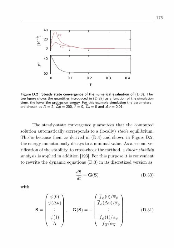
175
0
20
40
[10−5]
εψ
εΛ
-60
-40
0 0.1 0.2 0.3 0.4
F∗
t
Figure D.2 | Steady state convergence of the numerical evaluation of (D.3). Thetop figure shows the quantities introduced in (D.28) as a function of the simulationtime, the lower the protrusion energy. For this example simulation the parametersare chosen as Ω = 2, ∆p = 200, f = 0, C 0 = 0 and ∆u = 0.01.
The steady-state convergence guarantees that the computedsolution automatically corresponds to a (locally) stable equilibrium.This is because then, as derived in (D.4) and shown in Figure D.2,the energy monotonously decays to a minimal value. As a second ve-rification of the stability, to cross-check the method, a linear stabilityanalysis is applied in addition [193]. For this purpose it is convenientto rewrite the dynamic equations (D.3) in its discretized version as
dS
dt= G(S) (D.30)
with
S =
ψ(0)
ψ(∆u)...
ψ(1)
Λ
, G(S) = −
fψ(0)/αψfψ(∆u)/αψ
...fψ(1)/αψfΛ/αΛ
. (D.31)

176 Numerical solution for protrusion shapes J. Schneider
If S0 is a solution which satisfies the equilibrium shape equations,then S0 is a fixed point. The stability of this fixed point is determined,according to the linear stability analysis, by the Jacobian matrix
Jij :=∂Gi∂Sj
∣∣∣∣S0
. (D.32)
If the eigenvalues of J are all smaller than zero, then the system isstable at S0.
The evaluation of (D.32), performed here by an implementati-on in jacobiM.m, reveals that for the equilibrium solutions found inthis work all but two eigenvalues are negative. The two exceptionshave zero value, indicating that their corresponding eigenvectors giverise to equally favorable solutions. However, this can be understoodby the fact that the linear perturbation of the stability analysis viola-tes the two constraint conditions, (B.45) and (B.49), and hence thesenew solutions belong to different constraint values, one has an in-creased protrusion surface area and a decreased protrusion diameterthe other a decreased area and an increased diameter.
Reliability of the numerical solution
In order to ensure the reliability of the numerical results, obtainedwith the presented method and discussed in this work, several testsare utilized. First, it can be confirmed for every simulation that theconstraint conditions (B.45) on page 148 and (B.49) on page 149,which lead to the conditions in (D.12) for γ and µ0, are conservedthroughout the iterative equilibration. Second, as shown in Figu-re D.2 for one example, also the energy is found to always decaymonotonously, which is in agreement with (D.4).
Two further tests have been performed for some example si-mulations. One is the decrease of the spatial discretization size ∆u.

177
39.44
39.45
39.46
39.47
250 500 750 1000
γ
1/∆u
-2
-1
0
∂1/
∆uγ
Figure D.3 | Convergence of the numerical solution for a decreasing discretizationstep. Plotted is an example result of the simulation for the surface tension over theinverse spatial grid size. The used simulation parameters are Ω = 2, ∆p = 200,f = 0 and C 0 = 0. The inset shows the derivative of the main curve.
As expected, for a sufficiently small grid size the simulation resultsconverge to a constant value (see Figure D.2). For the other testthe equilibrium shape of the protrusion is separately calculated viathe Monge parameterization (see appendix B.2), using the same nu-merical procedure. From this it can be concluded that, as required,the simulation results are, indeed, invariant under parameterizationchanges. One example is shown in Figure D.4 where the results forelongation and surface tension of a protrusion calculated in both thearc length and the Monge parameterization are compared (gray solidline vs. dark gray crosses).
Besides the numerical testings, analytical approximations areprovided in this work to give an orientation of the trustworthiness ofthe numerical results (see, e.g., appendix E). In particular the weak-bending approximation of the Monge parameterization is of interest.It is introduced for protrusions with axial symmetry in appendix E.1and is plotted in addition to the full Monge parameterization andthe arc length parameterization in Figure D.4 (red dashed line). The

178 Numerical solution for protrusion shapes J. Schneider
0.10.20.30.40.50.6
L
-60
-40
-20
0.01 0.5
γ
Ω
Figure D.4 | Divergence of the analytical solution from the full numerical solutionfor increasing excess area. The solid gray line shows the elongation (top) and thesurface tension (bottom) as a function of the normalized protrusion area, obtainedwith the arc length parameterization. The dark gray crosses indicate the solutionsfor the Monge parameterization, the red dashed line these for the analyticalweak-bending approximation (see appendix E.1 and Figure E.1). The usedparameters are ∆p = 0, f = 0, C 0 = 0 and ∆u = 100 (arc length) and ∆ρ = 200(Monge), respectively.
elongation of the analytical weak-bending result approaches the fullsolution asymptotically as Ω → 0. This is in agreement with thedefinition of the weak-bending approximation, which only takes intoaccount weak variations of the height profile, as occurring for Ω ≈ 0.On the other hand, the surface tension diverges immediately, notasymptotically. It only agrees with the numerical result at Ω = 0
where γ is given by (E.19) on page 186. This can be clarified byusing the shape equation (B.17) on page 142 and solve it for γ:
γ = −f
(1)h
f(2)h
. (D.33)

179
Now, either f (1)h and f (2)
h can be expanded for weak height variationsfirst, as done in the weak-bending approximation, or its ratio can beexpanded directly. By doing so, the latter gives additional linearterms which do not appear in the first case. As, in turn, the lattercase reflects the behavior of the full Monge parameterization at Ω ≈0 this indicates that the weak-bending approximation seems to missrelevant information for the description of the surface tension, evenin the limit of weak bending.


APPENDIX
MEMBRANE PROTRUSIONSIN ANALYTICAL LIMITS E
In general, the equilibrium shapes of membrane protrusions as intro-duced and discussed in chapter 3 cannot be computed analytically.This is because in both the Monge parameterization and the arclength parameterization the obtained shape equations are stronglynonlinear. Whereas the numerical solution is discussed in appendixD, here three limits are discussed for which analytical results canbe found. The first is the weak-bending approximation, which hasbeen introduced in section 1.3.3. The second limit can be found forvanishing bending rigidity, κ→ 0. The third analytical limit can bediscussed for a non-vanishing point force f , applied to the tip of aprotrusion, which then adopts approximately the shape of cylindricalmembrane tubes.
E.1 | Weak-bending approximation
The shape equation (B.20) for h(ρ) in the weak-bending approxima-tion is linear with non-constant coefficients. It can firstly be rewrittenin dimensionless form with the help of the normalizations, introdu-
181

182 Membrane protrusions in analytical limits J. Schneider
ced in section 3.11. Secondly, (B.20) can immediately be integratedonce to
ρ2h|ρ ρ ρ + ρh|ρ ρ − (1 + γ∗ ρ2)h|ρ =∆p
2ρ3 −D1ρ, (E.1)
where the whole equation has been multiplied with ρ and D1 is thefirst integration constant. By introducing a new function h(ρ) suchthat h|ρ ≡ h+ D1
γ∗1ρ , (E.1) takes the following form:
ρ2h|ρ ρ + ρ h|ρ − (1 + γ∗ ρ2)h =∆p
2ρ3. (E.2)
A special solution for the inhomogeneous problem can be guessed as
hs = − 1
γ∗∆p
2ρ. (E.3)
The general solution of the remaining homogeneous problem can beobtained by performing the coordinate transformation ρ = iρ∗/
√γ∗.
The resulting equation
ρ∗2hh|ρ∗ρ∗ + ρ∗ hh|ρ∗ + ( ρ∗2 − 1)hh = 0 (E.4)
is, however, equivalent to the standard form of the first order Besselequation whose solutions are the Bessel function of first kind J1(γ∗)
and second kind Y1(γ∗) (also of first order) and their superpositionfor the general solution [214]
hh = D2J1 +D3Y1. (E.5)
1 The used normalizations are: ∆p := l3
κ∆p, f := l
κf C0 := l C0, γ := l2
κγ,
Ω := 4πl2
A − 1, F := 4F/πκ, V := 4V/πl3 and correspondingly h := hland
ρ := ρl.
E.1 Weak-bending approximation 183
Reverting the coordinate transformation and returning to the func-tion h by integrating once, the final solution of the initial shapeequation (B.20) becomes
h =D1 log ρ+D2J0(i√γ∗ρ)
+D3Y0(i√γ∗ρ) +D4 −
∆p
4γ∗ρ2, (E.6)
where D1, D2 and D3 have been redefined for convenience to absorboccurring constant prefactors.
In order to specify the solution (E.6) for a membrane protru-sion four boundary conditions are required. Those imposed in (3.2)on page 63 for the arc length parameterization give rise to threeconditions for the Monge parameterization, namely:
u = 0 : ρ =1
2& h = 0 ⇒ h(ρ =
1
2) = 0 (E.7)
& ψ = 0 ⇒ h|ρ(ρ =1
2) = 0, (E.8)
u = 1 : ρ = 0 & ψ = 0 ⇒ h|ρ(ρ = 0) = 0. (E.9)
The last two relations are due to
∂h
∂ρ=∂h
∂s
(∂ρ
∂s
)−1
= tanψψ1≈ ψ. (E.10)
A fourth relation can be deduced from the fact that at ρ = 0 theprincipal curvatures C1 and C2 have to be equal because of the axialsymmetry in this point. This leads to a differential equation for h:
ρ h|ρρ −(h|ρ − h
3|ρ
)= 0, (E.11)
where C1 and C2 were taken from the curvature tensor in Table B.1.The general solution of (E.11) describes the functional dependency

184 Membrane protrusions in analytical limits J. Schneider
of h(ρ) close to ρ = 02:
h ∝√
const.1 − ρ2 + const.2 . (E.12)
It implies for instance that besides the first derivative also the thirdderivative
h|ρ ρ ρ(ρ = 0) = 0. (E.13)
This means that the curvature along the contour line has to remaincontinuos at ρ = 0. Together with (E.9) this is only affordable forD1 = D3 = 0 of (E.6) as both related functions, the logarithmand the Bessel function of second kind, diverge at ρ = 0 and anynontrivial linear combination of these functions could not balancethis for both the first and third derivative. On the other hand, theremaining parts in (E.6) satisfy the two boundary conditions at ρ = 0
automatically as J0 ∝ 1 − ρ2
4 + ρ4
64 . The remaining two boundaryconditions specify D2 and D4 of (E.6) so that the final equilibriumshape of the membrane protrusion takes the form
h =∆p γ∗−3/2
4I1(√γ∗/2)
[I0(√γ∗ρ)− I0(
√γ∗/2)
+√γ∗(1/4− ρ2
)I1(√γ∗/2)
],
(E.14)
where I0 and I1 are the zeroth and first order modified Bessel func-tions of first kind, respectively3.
To determine the surface tension γ∗ by the imposed excessarea Ω of the protrusion the same strategy as presented at the endof appendix C can be applied. The excess area in the weak-bendingapproximation is given, according to the area element in Table B.1,
2 Replacing h|ρ = g in (E.11) leads to a separable equation, which can be integra-ted immediately.
3 They are related to the Bessel functions of first kind in the following way: Iα(x) =i−αJα(ix).
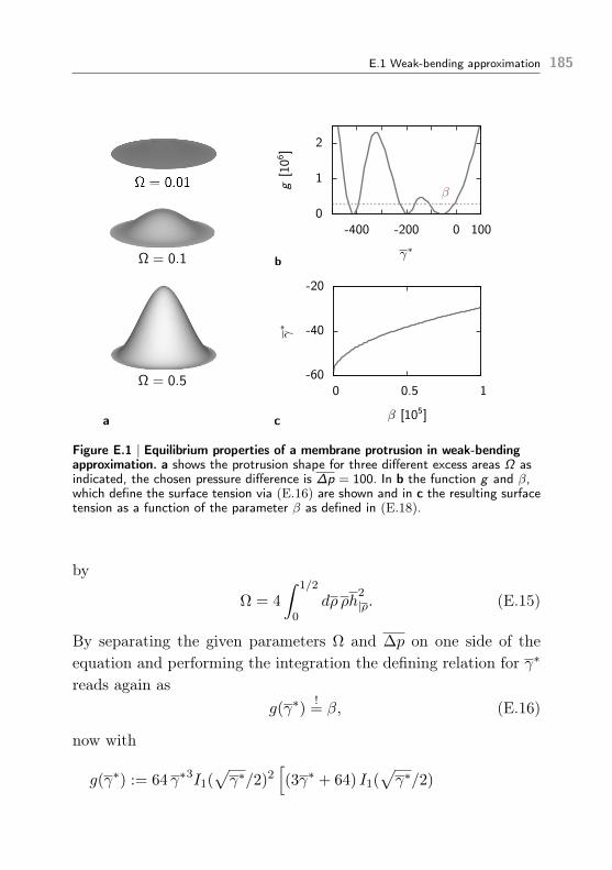
E.1 Weak-bending approximation 185
a
b
-60
-40
-20
0 0.5 1
γ∗
β [105]
0
1
2
-400 -200 0 100
g[106]
γ∗
β
c
Figure E.1 | Equilibrium properties of a membrane protrusion in weak-bendingapproximation. a shows the protrusion shape for three different excess areas Ω asindicated, the chosen pressure difference is ∆p = 100. In b the function g and β,which define the surface tension via (E.16) are shown and in c the resulting surfacetension as a function of the parameter β as defined in (E.18).
by
Ω = 4
∫ 1/2
0dρ ρh
2|ρ. (E.15)
By separating the given parameters Ω and ∆p on one side of theequation and performing the integration the defining relation for γ∗
reads again asg(γ∗)
!= β, (E.16)
now with
g(γ∗) := 64 γ∗3I1(√γ∗/2)2
[(3γ∗ + 64) I1(
√γ∗/2)

186 Membrane protrusions in analytical limits J. Schneider
−8γ∗I1(√γ∗/2)I0(
√γ∗/2)− 2γ∗I0(
√γ∗/2)2
]−1(E.17)
and β as defined previously
β :=∆p
2
Ω. (E.18)
The function g(γ∗) is plotted together with the intersecting line βin Figure E.1b. It exhibits very similar features as those found fora membrane sheet at the end of appendix C. Likewise, (E.16) canonly be solved numerically and the resulting surface tension γ∗(β)
is shown in Figure E.1c, as well as three example equilibrium shapes(Figure E.1a). Here the same assumptions regarding the choice of thebranch at γ∗ < 0 as for a membrane sheet are made. The minimalsurface tension at β = 0 is defined by the first root of the Besselfunction of first kind:
γ∗0 = 4(min J−1
1 (0))2
, (E.19)
where J−1α (0) are the roots of the respective Bessel function. For
large values of β, (E.17) goes asymptotically as the quadrat of thesurface tension, g ∝ 64 γ∗2, as also found before in appendix C. Oneadditional analytical result can be computed here for the specialpoint γ∗ = 0. There g(0) = 393216 what specifies the ratio of ∆p toΩ at which the surface tension vanishes.
E.2 | Zero-rigidity approximation
Setting κ = 0 the energy (B.5) reduces to a sum of the area termand volume term. In this form the energy gives rise to Laplace’s law,which connects the (constant) curvature radius r of a membranewith the pressure difference ∆p and the surface tension γ of the

E.2 Zero-rigidity approximation 187
Figure E.2 | Schematic of a membraneprotrusion approximated by a spherical cap.
membrane in the following way [103,104]:
r = 2γ
∆p. (E.20)
For a membrane protrusion with axial symmetry this means that itcan be described for κ → 0 by a spherical cap [170]. Such a cap issketched in Figure E.2. The surface tension in (E.20) is set by theimposed surface area A of the cap, which can be computed here, e.g.,in spherical coordinates:
A = r2
∫ 2π
0dϕ
∫ ψmax
0dψ sinψ = 2πr2 (1− cosψmax) , (E.21)
where the used maximal polar angle ψmax is defined by the protrusiondiameter l:
ψmax := arcsin (l/2r). (E.22)
Plugging (E.22) and (E.21) into (E.20) and solve this for γ gives
γ =∆p
2πl
A√4Aπl2− 1
. (E.23)
In dimensionless form and using the excess area Ω = 4A/πl2− 1 theradius r, the surface tension γ and the encapsulated volume V read
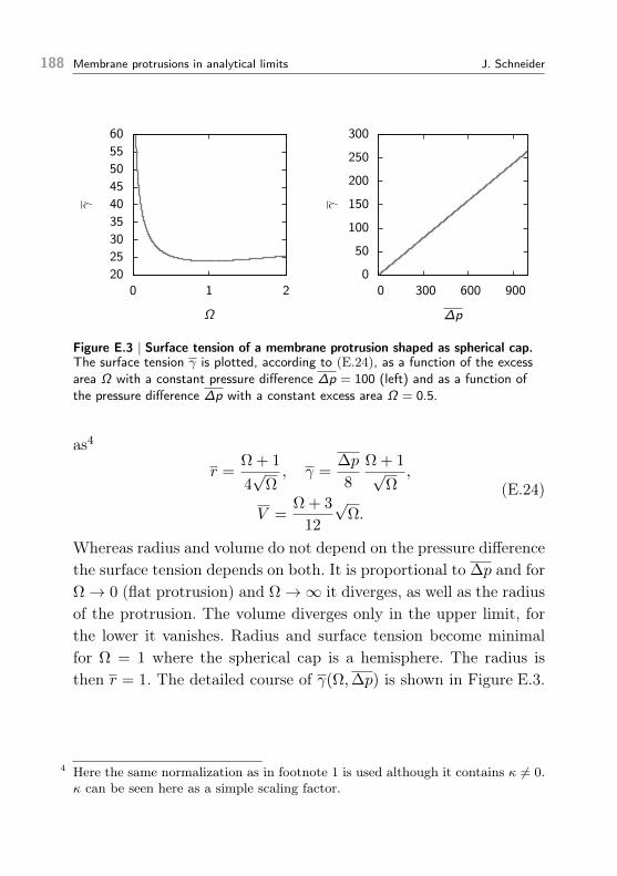
188 Membrane protrusions in analytical limits J. Schneider
202530354045505560
0 1 2
γ
Ω
0
50
100
150
200
250
300
0 300 600 900
γ∆p
Figure E.3 | Surface tension of a membrane protrusion shaped as spherical cap.The surface tension γ is plotted, according to (E.24), as a function of the excessarea Ω with a constant pressure difference ∆p = 100 (left) and as a function ofthe pressure difference ∆p with a constant excess area Ω = 0.5.
as4
r =Ω + 1
4√
Ω, γ =
∆p
8
Ω + 1√Ω
,
V =Ω + 3
12
√Ω.
(E.24)
Whereas radius and volume do not depend on the pressure differencethe surface tension depends on both. It is proportional to ∆p and forΩ→ 0 (flat protrusion) and Ω→∞ it diverges, as well as the radiusof the protrusion. The volume diverges only in the upper limit, forthe lower it vanishes. Radius and surface tension become minimalfor Ω = 1 where the spherical cap is a hemisphere. The radius isthen r = 1. The detailed course of γ(Ω, ∆p) is shown in Figure E.3.
4 Here the same normalization as in footnote 1 is used although it contains κ 6= 0.κ can be seen here as a simple scaling factor.

E.3 Tube approximation 189
Figure E.4 | Schematic of a cylindricalmembrane tube.
E.3 | Tube approximation
When membrane is pulled into a tube it can be modeled, in a goodapproximation, as a cylinder [116,191]. This approximation is, com-pared to the two previous approximations, strictly speaking not rigo-rous in the mathematical sense because it neglects the bottom partof the protrusion where it is attached to the base. Here this region isinstead treated as a flat disc. Then the simplified cross section of themembrane tube takes a form as shown in Figure E.4. The bottomdisc as well as the disc at the top of the cylinder do not contributeto the energy of the tube since their curvature is zero. Therefore,recalling volume and side area of a cylinder, the energy (B.5) can bewritten as5
F =
[κ
2
1
ρ2+ γ
]2πρL−∆pπρ2L− fL. (E.25)
In order to find the equilibrium cylinder shape (E.25) needs to beminimized with respect to both ρ and L. This gives rise to the twoequations
0 = ∆pρ3 − γ ρ2 +1
2, (E.26)
5 Area and volume of a cylinder can also be calculated with the help of the ex-pressions in Table B.1 taking into account that ρ is constant.

190 Membrane protrusions in analytical limits J. Schneider
0 = ∆pρ3 − 2γ ρ2 +f
πρ− 1, (E.27)
where now the same normalized quantities are used as previouslyfor axisymmetric protrusions. A third equation is given by the areaconservation, which is considered for the excess area as before:
Ω = 8ρL. (E.28)
The three equations match the three quantities ρ, L and γ and can,thus, be solved to express the unknowns by the given parameters ∆p
and f .To solve (E.26), (E.27) and (E.28) for radius, elongation and
surface tension, first, (E.26) and (E.28) can be solved for γ and L,respectively:
γ =2∆p ρ3 + 1
2ρ2 , (E.29)
L =Ω
8ρ. (E.30)
Both still depend on ρ. However, ρ can be determined independentlyby using (E.29) to eliminate γ in (E.27). This gives an equation thatonly depends on the radius:
0 = ∆p ρ3 − f
πρ+ 2. (E.31)
The solution can be derived by standard techniques for cubic equati-ons [215]. From the three occurring solutions only one is of physicalrelevance, namely
ρ = 6πζ−1tube
fsin
[arcsin ζtube
3
](E.32)

E.3 Tube approximation 191
with
ζtube :=
√27π3∆p
f3 (E.33)
being a dimensionless parameter, which has to lie in the range
0 ≤ ζtube ≤ 1. (E.34)
The upper boundary is required to ensure that ρ is real valued, thelower boundary is due to the fact that both the pressure differenceand the point force shall be equal or larger than zero here. The radiusmultiplied with the point force is plotted as a function of ζtube inFigure E.5a. It is monotonously increasing between 2π at ζtube = 0
and 3π at ζtube = 1.The result (E.32) together with (E.29) and (E.30) fully cha-
racterizes the equilibrium shape of a membrane tube, simplified bya cylinder. It is interesting to emphasize that neither the radius ofthe cylindrical tube nor the surface tension depends on the imposedarea. The elongation, on the other hand, is directly proportional tothe excess area. The pressure difference acts in all cases as a resca-ling parameter for the point force. This becomes more obvious byrewriting ζtube as
f
f tube= ζ
−2/3tube (E.35)
withf tube := 3π
3
√∆p . (E.36)
Nevertheless, f tube, and therewith ∆p, is not only a scaling para-meter but, according to the upper limit of ζtube in (E.34), also theminimal point force needed to induce tubes. The quantities ρ, L andγ cannot be expressed only in terms of the rescaled point force in(E.35) but the expressions ρf , L/Ωf and γ/f2. The latter two are

192 Membrane protrusions in analytical limits J. Schneider
2π
3π
0 1
ρf
ζtubea
124π
116π
1
L/
Ωf
f /f tubeb
18π2
16π2
1
γ/
f2
f /f tubec
Figure E.5 | Equilibrium properties of a cylindrical membrane tube. a shows thetube radius as in (E.32), multiplied with the point force. In b the elongation,divided by the imposed excess area and point force, is shown and in c the surfacetension, divided by the squared point force, both plotted as a function of therescaled point force (see text). The dashed lines indicate the ranges, according to(E.34), within which the three quantities are defined.
shown in Figure E.5b and Figure E.5c, respectively. Whereas L/Ωfincreases monotonously, starting from a minimal value at f = f tube,indicated in the plot, γ/f2 decays monotonously, also starting fromf = f tube. Especially interesting is the asymptotic behavior of bothfor f/f tube 1. Both expressions then approach a constant value,from which can be concluded that
L ∝ Ωf
16π, γ ∝ 1
2
(f
2π
)2
for f 3
√∆p . (E.37)

APPENDIX
ALTERNATIVELATERAL TENSION EXPRESSION F
In this work the lateral tension is defined as
γ‖ :=dFdA‖
, (F.1)
where F is the energy (B.5) on page 138 of the membrane and A‖ itsbasal area1. Calculating γ‖ according to (F.1) is inconvenient as itrequires first the integration of the equilibrium membrane shape tocompute F and then the differentiation. This procedure can becomecomputationally relatively costly and also inaccurate if a numericalcalculation is involved.
An alternative approach to obtain the lateral tension γ‖ isto study the work dW needed to deform the membrane such thatthe basal area changes by dA‖. This can be done because here theinfinitesimal work performed is equal to the negative infinitesimalchange of the energy:
dW = −dF = −γ‖dA‖. (F.2)
1 The basal area A‖ is the projection of the membrane area into the x-y-plane.
193

194 Alternative lateral tension expression J. Schneider
On the other hand dW can be written as the surface integral2
dW =
∫dAγijdεi|j (F.3)
over the scalar product of the gradient of local displacements dεi andthe local, tangential tension tensor [216]3
γij =κ
2(Ckk − C0)
(2Cki gjk − (Ckk − C0) gij
)− γ gij . (F.4)
Equation (F.3) can be rewritten by using the chain rule and forcebalance γij|j = 0 so that the divergence theorem [214] can be applied:
dW =
∫dA(γijdεi
)|j =
∮dΓ νjγ
ijdεi. (F.5)
The second integration is performed along the closed boundary line Γ
of the membrane where νj is the unit normal vector of the boundaryline. If the local displacement dεi acts isotropically in perpendicularto the boundary line, then it is, on the one hand, independent of thepath integration in (F.5) and, on the other hand, can be written asdεi = dε νi. Taking this into account in (F.5) together with (F.2) thefollowing relation for the lateral tension can be found4:
γ‖ = −(dA‖
dε
)−1 ∮dΓνiνjγij . (F.6)
Relation (F.6) can further be simplified for specific membranegeometries. Here it is used for membrane protrusions, as discussed inthis work. Their axial symmetry is resulting from the full and smoothattachment along the circular boundary line at constant radius ρ =
l/2. The basal area is, hence, A‖ = π4 l
2 and the deformation dε =
2 Again the simplification |i := ∂/∂xi is used here.3 γij is tangential to the surface.4 Here the indices of νiνj and γij were flipped for convenience.

195
dl/2 acts in radial direction (due to the smooth boundary). Theboundary path Γ can be parameterized by the polar angle as dΓ =l2dϕ. Equation (F.6) then simplifies to
γ‖ = − 1
2π
∫dϕ γρρ
∣∣∣∣ρ= l
2
. (F.7)
As the membrane protrusion is axisymmetric γρρ does not depend onthe integration with respect to ϕ. That simplifies the lateral tensionto γ‖ = −γρρ. Furthermore, taking into account that at the boundaryline gρρ = gss = bs ·bs = 1, gϕs = gϕρ = bϕ ·bs = 0 and Cϕϕ = 0, therequired tensor component γρρ can be calculated so that the lateraltension for a membrane protrusion becomes
γ‖ =[γ∗ − κ
2(2H)2
]ρ= l
2
. (F.8)
Here the mean curvature is equivalent toH = 12C
ρρ. The found result
agrees with what has been reported in [192] and [139].

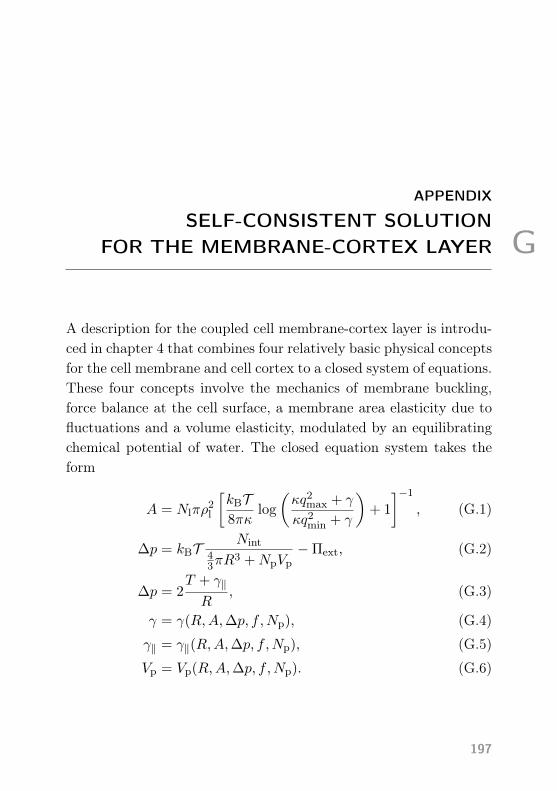
APPENDIX
SELF-CONSISTENT SOLUTIONFOR THE MEMBRANE-CORTEX LAYER G
A description for the coupled cell membrane-cortex layer is introdu-ced in chapter 4 that combines four relatively basic physical conceptsfor the cell membrane and cell cortex to a closed system of equations.These four concepts involve the mechanics of membrane buckling,force balance at the cell surface, a membrane area elasticity due tofluctuations and a volume elasticity, modulated by an equilibratingchemical potential of water. The closed equation system takes theform
A = Nlπρ2l
[kBT8πκ
log
(κq2
max + γ
κq2min + γ
)+ 1
]−1
, (G.1)
∆p = kBTNint
43πR
3 +NpVp−Πext, (G.2)
∆p = 2T + γ‖
R, (G.3)
γ = γ(R,A, ∆p, f ,Np), (G.4)
γ‖ = γ‖(R,A, ∆p, f ,Np), (G.5)
Vp = Vp(R,A, ∆p, f ,Np). (G.6)
197

198 Self-consistent solution for the membrane-cortex layer J. Schneider
Here Nl is the number of lipids, Np the number of protrusions, Nint
the number of solute particles inside the cell, Πext the external os-motic pressure, T the cortex tension and f a local force exertedby cortex filaments onto the cell membrane. If these quantities areknown, this equation system determines the global cell propertiespressure difference ∆p, surface tension γ, radius R, volume V andsurface area A self-consistently.
Numerical solution
The equation system (G.1) – (G.6) can, in general, only be solvednumerically. This is, on the one hand, owed the fact that the fullinformation on membrane buckling, given by the relations (G.4),(G.5) and (G.6), is obtained numerically (see chapter 3 and appendixD for details). On the other hand, relation (G.1) would lead, inany case, to a transcendental relation, which can only be solvedimplicitly. However, the equation system can be simplified for thenumerical evaluation because for the quantities γ, γ‖ and Vp explicitexpressions are known. Hence, only three equations must be solvedsimultaneously. They can be obtained by plugging (G.4) into (G.1),(G.5) into (G.3) and (G.6) into (G.2). For this work the remainingset of equations is solved with the built-in function FindRoot ofMathematica. Furthermore, with the function Interpolation thenumerical results for γ, γ‖ and Vp are interpolated in order to enablethe numerical evaluation.
Analytical solution for zero cortex tension
For zero cortex tension, T = 0, on the one hand, the force balance(G.3) turns into Laplace’s law, relating the cell radius R0 and lateralmembrane tension γ‖0 to the cell pressure ∆p0. On the other hand, if

199
cap
Figure G.1 | Schematic of thegeometrical relations between sphericalcap membrane protrusion and cell cortex.R0 is the apparent cell radius, r0 the capradius, γ0 the membrane surface tension,γ‖0 the lateral membrane tension and ψ0,ψ′0 tilt angles between the tensions andthe ρ-axis.
the membrane protrusions, which form due to buckling, are treatedas spherical caps (see section E.2), also each protrusion has to obeyLaplace’s law in the form (E.20) on page 187, relating the protrusionradius r0 and membrane surface tension γ0 to the pressure difference∆p′0. Since the pressure difference has to take the same value in both
cases, i.e., ∆p0 = ∆p′0, it follows:
γ
r0=γ‖0R0
= cos (ψ0 − ψ′0)γ0
R0. (G.7)
Here γ‖0 is projected to the spherical cortex (see Figure G.1). Equa-tion (G.7) can only be satisfied if R0 = r0 and ψ0 = ψ
′0. That means
the cap becomes a portion of the underlying sphere or, in otherwords, the cell membrane does not buckle for T = 0.
For an unbuckled membrane which is flat attached to the un-derlying cortex the equation system (G.1) – (G.6) becomes particu-larly simple as then Vp = 0 and γ0 = γ‖0 . Hence, ∆p0 in (G.2) canbe replaced via (G.3) by R0 and γ0. Furthermore, A0 = 4πR2
0 andV0 = 4πR3
0/3 in (G.1) and (G.2), respectively. Equations (G.2) canthen be solved for the surface tension
γ0 =3kBT Nint − 4πR3
0 Πext
8πR20
(G.8)

200 Self-consistent solution for the membrane-cortex layer J. Schneider
and R0 is implicitly determined via (G.1) by the relation
Nlρ2l
4R20
= 1 +kBT8πκ
log
[3kBT Nint + 8πκq2
maxR20 − 4πΠextR
30
3kBT Nint + 8πκq2minR
20 − 4πΠextR3
0
].
(G.9)
Area and volume elasticity for small cortex tensions
In contrast to the case T = 0, where the cell membrane is flat atta-ched to the underlying cortex, for T > 0 the numerical solution of(G.1) – (G.6) predicts for biological relevant parameters a bucklingof the cell membrane into small protrusions. This is discussion inmore detail in section 4.2.2. There it is also stated that in order toenable buckling it is necessary that the cell exhibits a finite volumeor area elasticity, represented by (G.1) and (G.2), respectively. Forvery small cortex tensions these elasticities can be estimated ana-lytically by expanding (G.1) and (G.2) around the initial sphericalshape. The result can be written in the form
γ ≈ γ0 +KAA0 −AA0
, (G.10)
∆p ≈ ∆p0 +KVV0 − VV0
(G.11)
with the respective area elasticity and volume elasticity
KA := −καAb
A0
(q2max − q2
min)eα(1+Ab/A0)(
eα − eαAb/A0)2 , (G.12)
KV := kBTNint
V0, (G.13)
where α := 8πκ/kBT and Ab = Nlπρ2l . The quantities A0, V0, γ0
and ∆p0 correspond to those found in the limit T → 0.

REFERENCES
[1] G. W. C. Kaye and T. H. Laby. Tables of physical and chemical constants.Longman, Harlow, 16th ed. (1995)
[2] H. Goldmann. Spaltlampenphotographie und –photometric. Ophthalmolo-gica 98, 257–270 (1939)
[3] A. Nwaneshiudu, C. Kuschal, F. H. Sakamoto, R. R. Anderson, K. Schwar-zenberger, and R. C. Young. Introduction to confocal microscopy. Journalof Investigative Dermatology 132, e3 (2012)
[4] P. Vesely. Handbook of biological confocal microscopy. Scanning 29, 91–91(2007)
[5] D. Kruger, P. Schneck, and H. Gelderblom. Helmut ruska and the visua-lisation of viruses. The Lancet 355, 1713–1717 (2000)
[6] H. G. Rudenberg and P. G. Rudenberg. Chapter 6 - Origin and backgroundof the invention of the electron microscope: Commentary and expanded no-tes on memoir of reinhold rüdenberg. In Advances in Imaging and ElectronPhysics, 207–286. Elsevier (2010)
[7] R. F. Egerton. Physical principles of electron microscopy: an introductionto TEM, SEM, and AEM. Springer, New York (2005)
[8] R. Hooke, J. Martyn, and J. Allestry. Micrographia or some physiologicaldescriptions of minute bodies made by magnifying glasses with observationsand inquiries thereupon. Royal Society (1665)
[9] B. Alberts, A. Johnson, J. Lewis, M. Raff, K. Roberts, and P. Walter.Molecular biology of the cell. Garland Science, 4th ed. (2002)
[10] C. R. Woese, O. Kandler, and M. L. Wheelis. Towards a natural systemof organisms: proposal for the domains archaea, bacteria, and eucarya.Proceedings of the National Academy of Sciences 87, 4576–4579 (1990)
201

202 References J. Schneider
[11] A. G. Clark, K. Dierkes, and E. K. Paluch. Monitoring actin cortex thick-ness in live cells. Biophysical Journal 105, 570–580 (2015)
[12] J. Hanson and J. Lowy. The structure of f-actin and of actin filamentsisolated from muscle. Journal of Molecular Biology 6, 46–60 (1963)
[13] N. Morone, T. Fujiwara, K. Murase, R. S. Kasai, H. Ike, S. Yuasa, J. Usu-kura, and A. Kusumi. Three-dimensional reconstruction of the membraneskeleton at the plasma membrane interface by electron tomography. TheJournal of Cell Biology 174, 851–862 (2006)
[14] G. Charras, C.-K. Hu, M. Coughlin, and T. Mitchison. Reassembly ofcontractile actin cortex in cell blebs. Journal of Cell Biology 175, 477–490(2006)
[15] F. Gittes, B. Mickey, J. Nettleton, and J. Howard. Flexural rigidity ofmicrotubules and actin filaments measured from thermal fluctuations inshape. The Journal of Cell Biology 120, 923–934 (1993)
[16] G. Salbreux, G. Charras, and E. Paluch. Actin cortex mechanics andcellular morphogenesis. Trends in Cell Biology (2012)
[17] M. Fritzsche, A. Lewalle, T. Duke, K. Kruse, and G. Charras. Analysis ofturnover dynamics of the submembranous actin cortex. Molecular Biologyof the Cell 24, 757–767 (2013)
[18] H. Miyata, R. Yasuda, and K. Kinosita Jr. Strength and lifetime of thebond between actin and skeletal muscle α-actinin studied with an opticaltrapping technique. Biochimica et Biophysica Acta 1290, 83–88 (1996)
[19] S. Mukhina, Y. li Wang, and M. Murata-Hori. α-actinin is required fortightly regulated remodeling of the actin cortical network during cytokinesis.Developmental Cell 13, 554–565 (2007)
[20] D. Bray and J. White. Cortical flow in animal cells. Science 239, 883–888(1988)
[21] O. Thoumine and A. Ott. Time scale dependent viscoelastic and contractileregimes in fibroblasts probed by microplate manipulation. Journal of CellScience 110, 2109–2116 (1997)
[22] G. Forgacs, R. A. Foty, Y. Shafrir, and M. S. Steinberg. Viscoelasticproperties of living embryonic tissues: a quantitative study. BiophysicalJournal 74, 2227–2234 (1998)
[23] M. J. Tyska and D. M. Warshaw. The myosin power stroke. Cell Motilityand the Cytoskeleton 51, 1–15 (2002)

References 203
[24] J. Peukes and T. Betz. Direct measurement of the cortical tension duringthe growth of membrane blebs. Biophysical Journal 107, 1810–1820 (2014)
[25] M. Mayer, M. Depken, J. S. Bois, F. Julicher, and S. W. Grill. Anisotro-pies in cortical tension reveal the physical basis of polarizing cortical flows.Nature 467, 617–621 (2010)
[26] J. Sedzinski, M. Biro, A. Oswald, J.-Y. Tinevez, G. Salbreux, and E. Pa-luch. Polar actomyosin contractility destabilizes the position of the cytoki-netic furrow. Nature 476, 462–466 (2011)
[27] J.-F. Joanny and J. Prost. Active gels as a description of the actin-myosincytoskeleton. Human Frontier Science Program Journal 3, 94–104 (2009)
[28] A. G. Clark, O. Wartlick, G. Salbreux, and E. K. Paluch. Stresses atthe cell surface during animal cell morphogenesis. Current Biology 24,R484–R494 (2014)
[29] F. C. Sauer. Mitosis in the neural tube. The Journal of ComparativeNeurology 62, 377–405 (1935)
[30] M. P. Stewart, J. Helenius, Y. Toyoda, S. P. Ramanathan, D. J. Muller,and A. A. Hyman. Hydrostatic pressure and the actomyosin cortex drivemitotic cell rounding. Nature 469, 226–230 (2011)
[31] S. P. Ramanathan, J. Helenius, M. P. Stewart, C. J. Cattin, A. A. Hyman,and D. J. Muller. Cdk1-dependent mitotic enrichment of cortical myosinii promotes cell rounding against confinement. Nature Cell Biology 17,148–159 (2015)
[32] G. Charras and E. Paluch. Blebs lead the way: how to migrate withoutlamellipodia. Nature Reviews Molecular Cell Biology 9, 730–736 (2008)
[33] M. Bergert, A. Erzberger, R. A. Desai, I. M. Aspalter, A. C. Oates,G. Charras, G. Salbreux, and E. K. Paluch. Force transmission duringadhesion-independent migration. Nature Cell Biology 17, 524–529 (2015)
[34] S. R. Naganathan, S. Fürthauer, M. Nishikawa, F. Jülicher, and S. W.Grill. Active torque generation by the actomyosin cell cortex drives left–right symmetry breaking. eLife 3 (2014)
[35] R. Farhadifar, J.-C. Röper, B. Aigouy, S. Eaton, and F. Jülicher. The influ-ence of cell mechanics, cell-cell interactions, and proliferation on epithelialpacking. Current Biology 17, 2095–2104 (2007)
[36] R. Etournay, M. Popović, M. Merkel, A. Nandi, C. Blasse, B. Aigouy,H. Brandl, G. Myers, G. Salbreux, F. Jülicher, S. Eaton, and H. McNeill.

204 References J. Schneider
Interplay of cell dynamics and epithelial tension during morphogenesis ofthe drosophila pupal wing. eLife (2015)
[37] K. Dierkes, A. Sumi, J. Solon, and G. Salbreux. Spontaneous oscillationsof elastic contractile materials with turnover. Physical Review Letters 113,148102 (2014)
[38] L. Saias, J. Swoger, A. D’Angelo, P. Hayes, J. Colombelli, J. Sharpe, G. Sal-breux, and J. Solon. Decrease in cell volume generates contractile forcesdriving dorsal closure. Developmental Cell 33, 611–621 (2015)
[39] G. Karp. Cell and molecular biology: concepts and experiments. Wiley,Hoboken, 5th ed. (2008)
[40] A. Krogh, B. Larsson, G. von Heijne, and E. L. Sonnhammer. Predictingtransmembrane protein topology with a hidden markov model: applicationto complete genomes. Journal of Molecular Biology 305, 567–580 (2001)
[41] B. Hille. Ion channels of excitable membranes. Sinauer Assoc., Sunderland,Mass., 3rd ed. (2001)
[42] S. Mukherjee, R. N. Ghosh, and F. R. Maxfield. Endocytosis. PhysiologicalReviews 77, 759–803 (1997)
[43] B. Razani, S. E. Woodman, and M. P. Lisanti. Caveolae: From cell biologyto animal physiology. Pharmacological Reviews 54, 431–467 (2002)
[44] M. Algrain, O. Turunen, A. Vaheri, D. Louvard, and M. Arpin. Ezrincontains cytoskeleton and membrane binding domains accounting for itsproposed role as a membrane-cytoskeletal linker. The Journal of Cell Bio-logy 120, 129–139 (1993)
[45] R. G. Fehon, A. I. McClatchey, and A. Bretscher. Organizing the cellcortex: the role of erm proteins. Nature Reviews Molecular Cell Biology11, 276–287 (2010)
[46] M. P. Sheetz. Cell control by membrane–cytoskeleton adhesion. NatureReviews Molecular Cell Biology 2, 392–396 (2001)
[47] M. Fritzsche, R. Thorogate, and G. Charras. Quantitative analysis of ezrinturnover dynamics in the actin cortex. Biophysical Journal 106, 343–353(2014)
[48] F. Brochard and J. Lennon. Frequency spectrum of the flicker phenomenonin erythrocytes. J. Phys. France 36, 1035–1047 (1975)
[49] E. Sackmann, J. Engelhardt, K. Fricke, and H. Gaub. On dynamic mo-lecular and elastic properties of lipid bilayers and biological membranes.Colloids and Surfaces 10, 321–335 (1984)

References 205
[50] T. Betz and C. Sykes. Time resolved membrane fluctuation spectroscopy.Soft Matter 8, 5317–5326 (2012)
[51] S. Levin and R. Korenstein. Membrane fluctuations in erythrocytes arelinked to mgatp-dependent dynamic assembly of the membrane skeleton.Biophysical Journal 60, 733–737 (1991)
[52] S. Tuvia, S. Levin, A. Bitler, and R. Korenstein. Mechanical fluctuati-ons of the membrane–skeleton are dependent on f-actin atpase in humanerythrocytes. The Journal of Cell Biology 141, 1551–1561 (1998)
[53] J.-B. Manneville, P. Bassereau, S. Ramaswamy, and J. Prost. Active mem-brane fluctuations studied by micropipet aspiration. Physical Review E 64,021908 (2001)
[54] N. Gov. Membrane undulations driven by force fluctuations of active pro-teins. Physical Review Letters 93, 268104 (2004)
[55] A. C. Woodka, P. D. Butler, L. Porcar, B. Farago, and M. Nagao. Li-pid bilayers and membrane dynamics: Insight into thickness fluctuations.Physical Review Letters 109, 058102 (2012)
[56] H. M. McConnell and R. D. Kornberg. Inside-outside transitions of phos-pholipids in vesicle membranes. Biochemistry 10, 1111–1120 (1971)
[57] F. Kamp and J. A. Hamilton. ph gradients across phospholipid membra-nes caused by fast flip-flop of un-ionized fatty acids. Proceedings of theNational Academy of Sciences 89, 11367–11370 (1992)
[58] F. Kamp, D. Zakim, F. Zhang, N. Noy, and J. A. Hamilton. Fatty acidflip-flop in phospholipid bilayers is extremely fast. Biochemistry 34, 11928–11937 (1995)
[59] T. Fujiwara, K. Ritchie, H. Murakoshi, K. Jacobson, and A. Kusumi. Phos-pholipids undergo hop diffusion in compartmentalized cell membrane. TheJournal of Cell Biology 157, 1071–1082 (2002)
[60] G. Lindblom and G. Orädd. Lipid lateral diffusion and membrane hetero-geneity. Biochimica et Biophysica Acta 1788, 234–244 (2009)
[61] J. Lippincott-Schwartz, E. Snapp, and A. Kenworthy. Studying proteindynamics in living cells. Nature Reviews Molecular Cell Biology 2, 444–456 (2001)
[62] K. Schmidt and B. J. Nichols. A barrier to lateral diffusion in the cleavagefurrow of dividing mammalian cells. Current Biology 14, 1002–1006 (2004)

206 References J. Schneider
[63] S. J. Singer and G. L. Nicolson. The fluid mosaic model of the structureof cell membranes. Science 175, 720–731 (1972)
[64] A. Kusumi and Y. Sako. Cell surface organization by the membrane ske-leton. Current Opinion in Cell Biology 8, 566–574 (1996)
[65] A. Kusumi, C. Nakada, K. Ritchie, K. Murase, K. Suzuki, H. Murakoshi,R. S. Kasai, J. Kondo, and T. Fujiwara. Paradigm shift of the plasma mem-brane concept from the two-dimensional continuum fluid to the partitionedfluid: High-speed single-molecule tracking of membrane molecules. AnnualReview of Biophysics and Biomolecular Structure 34, 351–378 (2005)
[66] K. Suzuki, K. Ritchie, E. Kajikawa, T. Fujiwara, and A. Kusumi. Rapidhop diffusion of a g-protein-coupled receptor in the plasma membrane asrevealed by single-molecule techniques. Biophysical Journal 88, 3659–3680(2005)
[67] R. D. Allen. Fine structure of membranous and microfibrillar systems inthe cortex of paramecium caudatum. The Journal of Cell Biology 49, 1–20(1971)
[68] E. A. C. Follett and R. D. Goldman. The occurrence of microvilli duringspreading and growth of bhk21/c13 fibroblasts. Experimental Cell Research59, 124–136 (1970)
[69] S. J. Burwen and B. H. Satir. Plasma membrane folds on the mast cellsurface and their relationship to secretory activity. The Journal of CellBiology 74, 690–697 (1977)
[70] M. P. Sheetz, J. E. Sable, and H.-G. Döbereiner. Continuous membrane-cytoskeleton adhesion requires continuous accommodation to lipid and cy-toskeleton dynamics. Annual Review of Biophysics and BiomolecularStructure 35, 417–434 (2006)
[71] S. Mayor. Need tension relief fast? Try caveolae. Cell 144, 323–324 (2011)
[72] B. Sinha, D. Köster, R. Ruez, P. Gonnord, M. Bastiani, D. Abankwa, R. V.Stan, G. Butler-Browne, B. Vedie, L. Johannes, N. Morone, R. G. Parton,G. Raposo, P. Sens, C. Lamaze, and P. Nassoy. Cells respond to mechanicalstress by rapid disassembly of caveolae. Cell 144, 402–413 (2011)
[73] P. Sens and M. S. Turner. Budded membrane microdomains as tensionregulators. Physical Review E 73, 031918 (2006)
[74] D. Raucher and M. P. Sheetz. Characteristics of a membrane reservoirbuffering membrane tension. Biophysical Journal 77, 1992–2002 (1999)

References 207
[75] N. Groulx, F. Boudreault, S. Orlov, and R. Grygorczyk. Membrane reser-ves and hypotonic cell swelling. Journal of Membrane Biology 214, 43–56(2006)
[76] C. Morris and U. Homann. Cell surface area regulation and membranetension. Journal of Membrane Biology 179, 79–102 (2001)
[77] L. Figard and A. M. Sokac. A membrane reservoir at the cell surface:Unfolding the plasma membrane to fuel cell shape change. Bioarchitecture4, 39–46 (2014)
[78] R. M. Steinman, I. S. Mellman, W. A. Muller, and Z. A. Cohn. Endocytosisand the recycling of plasma membrane. The Journal of Cell Biology 96,1–27 (1983)
[79] J. Wolfe and P. L. Steponkus. Mechanical properties of the plasma mem-brane of isolated plant protoplasts: Mechanism of hyperosmotic and extra-cellular freezing injury. Plant Physiology 71, 276–285 (1983)
[80] E. Boucrot and T. Kirchhausen. Endosomal recycling controls plasmamembrane area during mitosis. Proceedings of the National Academy ofSciences 104, 7939–7944 (2007)
[81] L. Thilo and G. Vogel. Kinetics of membrane internalization and recy-cling during pinocytosis in dictyostelium discoideum. Proceedings of theNational Academy of Sciences of the United States of America 77 (1980)
[82] N. C. Gauthier, M. A. Fardin, P. Roca-Cusachs, and M. P. Sheetz. Tem-porary increase in plasma membrane tension coordinates the activation ofexocytosis and contraction during cell spreading. Proceedings of the Na-tional Academy of Sciences 108, 14467–14472 (2011)
[83] H. Harris. The Birth of the Cell. Yale University Press (2000)
[84] S. J. Morrison and J. Kimble. Asymmetric and symmetric stem-cell divi-sions in development and cancer. Nature 441, 1068–1074 (2006)
[85] H. T. K. Tse, W. M. Weaver, and D. Di Carlo. Increased asymmetric andmulti-daughter cell division in mechanically confined microenvironments.PLoS ONE 7, e38986 (2012)
[86] P. Kunda and B. Baum. The actin cytoskeleton in spindle assembly andpositioning. Trends in Cell Biology 19, 174–179 (2009)
[87] S. Carreno, I. Kouranti, E. S. Glusman, M. T. Fuller, A. Echard, andF. Payre. Moesin and its activating kinase slik are required for corticalstability and microtubule organization in mitotic cells. The Journal of CellBiology 180, 739–746 (2008)

208 References J. Schneider
[88] C. E. Walczak and R. Heald. Chapter 3 - Mechanisms of mitotic spindleassembly and function. In A Survey of Cell Biology, International Reviewof Cytology, vol. 265, 111–158. Academic Press (2008)
[89] J. Brugués and D. Needleman. Physical basis of spindle self-organization.Proceedings of the National Academy of Sciences 111, 18496–18500 (2014)
[90] C. Luxenburg, H. Amalia Pasolli, S. E. Williams, and E. Fuchs. Deve-lopmental roles for srf, cortical cytoskeleton and cell shape in epidermalspindle orientation. Nature Cell Biology 13, 203–214 (2011)
[91] O. M. Lancaster, M. L. Berre, A. Dimitracopoulos, D. Bonazzi, E. Zlotek-Zlotkiewicz, R. Picone, T. Duke, M. Piel, and B. Baum. Mitotic roundingalters cell geometry to ensure efficient bipolar spindle formation. Develop-mental Cell 25, 270 – 283 (2013)
[92] J. R. McIntosh, E. L. Grishchuk, and R. R. West. Chromosome-microtubule interactions durin mitosis. Annual Review of Cell and De-velopmental Biology 18, 193–219 (2002)
[93] S. Dumont. Chromosome segregation: Spindle mechanics come to life.Current Biology 21, R688–R690 (2011)
[94] L. G. Cao and Y. L. Wang. Signals from the spindle midzone are requiredfor the stimulation of cytokinesis in cultured epithelial cells. MolecularBiology of the Cell 7, 225–232 (1996)
[95] S. Oliferenko, T. G. Chew, and M. K. Balasubramanian. Positioning cy-tokinesis. Genes & Development 23, 660–674 (2009)
[96] C. Cabernard, K. E. Prehoda, and C. Q. Doe. A spindle-independentcleavage furrow positioning pathway. Nature 467, 91–94 (2010)
[97] T. E. Schroeder. Cell constriction: Contractile role of microfilaments indivision and development. American Zoologist 13, 949–960 (1973)
[98] L. G. Cao and Y. L. Wang. Mechanism of the formation of contractilering in dividing cultured animal cells. i. recruitment of preexisting actinfilaments into the cleavage furrow. The Journal of Cell Biology 110, 1089–1095 (1990)
[99] D. N. Robinson and J. A. Spudich. Towards a molecular understanding ofcytokinesis. Trends in Cell Biology 10, 228–237 (2000)
[100] K. Murthy and P. Wadsworth. Myosin-ii-dependent localization and dy-namics of f-actin during cytokinesis. Current Biology 15, 724–731 (2005)

References 209
[101] H. Turlier, B. Audoly, J. Prost, and J.-F. Joanny. Furrow constriction inanimal cell cytokinesis. Biophysical Journal 106, 114–123 (2014)
[102] W. Greiner, D. Rischke, L. Neise, and H. Stöcker. Thermodynamics andStatistical Mechanics. Springer, New York (2000)
[103] T. Young. An essay on the cohesion of fluids. Philosophical Transactionsof the Royal Society of London 95, 65–87 (1805)
[104] P. S. d. Laplace. Traité de mécanique céleste. Duprat, Paris (1799)
[105] S. K. Feller (Editor). Computational Modeling of Membrane Bilayers,vol. 60. Elsevier, Amsterdam (2008)
[106] P. B. Canham. The minimum energy of bending as a possible explanationof the biconcave shape of the human red blood cell. Journal of TheoreticalBiology 26, 61–81 (1970)
[107] S. Svetina and B. Zeks. Membrane bending energy and shape determi-nation of phospholipid vesicles and red blood cells. European BiophysicsJournal 17, 101–111 (1989)
[108] R. Lipowsky. The conformation of membranes. Nature 349, 475–481(1991)
[109] F. Jülicher. Die Morphologie von Vesikeln. Ph.D. thesis, University ofCologne (1994)
[110] W. Helfrich. Elastic properties of lipid bilayers: Theory and possible expe-riments. Zeitschrift für Naturforschung 28c, 693–703 (1973)
[111] E. A. Evans. Bending resistance and chemically induced moments in mem-brane bilayers. Biophysical Journal 14, 923–931 (1974)
[112] R. Dimova. Recent developments in the field of bending rigidity measu-rements on membranes. Advances in Colloid and Interface Science 208,225–234 (2014)
[113] W. Helfrich. Blocked lipid exchange in bilayers and its possible influence onthe shape of vesicles. Zeitschrift für Naturforschung 29c, 510–515 (1974)
[114] U. Seifert. Configurations of fluid membranes and vesicles. Advances inPhysics 46, 13–137 (1997)
[115] O.-Y. Zhong-can and W. Helfrich. Instability and deformation of a sphe-rical vesicle by pressure. Physical Review Letters 59, 2486–2488 (1987)
[116] I. Derényi, F. Jülicher, and J. Prost. Formation and interaction of mem-brane tubes. Physical Review Letters 88, 238101 (2002)

210 References J. Schneider
[117] E. Hannezo, J. Prost, and J.-F. Joanny. Mechanical instabilities of biolo-gical tubes. Physical Review Letters 109, 018101 (2012)
[118] M. Raatz, R. Lipowsky, and T. R. Weikl. Cooperative wrapping of nano-particles by membrane tubes. Soft Matter 10, 3570–3577 (2014)
[119] X. Liang, Y. Zu, Y.-P. Cao, and C. Yang. A dual-scale model for thecaveolin-mediated vesiculation. Soft Matter 9, 7981–7987 (2013)
[120] M. P. do Carmo. Differential geometry of curves and surfaces. PrenticeHall, Englewood Cliffs (1976)
[121] E. P. Petrov, S. Arumugam, J. Ehrig, and P. Schwille. Cytoskeletal pinningprevents large-scale phase separation in model membranes. BiophysicalJournal 104, 252a (2013)
[122] L. J. Pike. The challenge of lipid rafts. Journal of Lipid Research 50,S323–S328 (2009)
[123] E. Glassinger and R. M. Raphael. Influence of thermally driven surface un-dulations on tethers formed from bilayer membranes. Biophysical Journal91, 619–625 (2006)
[124] E. Evans and A. Yeung. Special issue functional dynamics of lipids in bio-membranes hidden dynamics in rapid changes of bilayer shape. Chemistryand Physics of Lipids 73, 39–56 (1994)
[125] U. Seifert and S. A. Langer. Viscous modes of fluid bilayer membranes.Europhysics Letters 23, 71 (1993)
[126] M. A. Peterson, H. Strey, and E. Sackmann. Theoretical and phase contrastmicroscopic eigenmode analysis of erythrocyte flicker: amplitudes. Journalde Physique II 2, 1273–1285 (1992)
[127] M. B. Schneider, J. T. Jenkins, and W. W. Webb. Thermal fluctuati-ons of large quasi-spherical bimolecular phospholipid vesicles. Journal dePhysique 45, 1457–1472 (1984)
[128] S. T. Milner and S. A. Safran. Dynamical fluctuations of droplet microe-mulsions and vesicles. Physical Review A 36, 4371–4379 (1987)
[129] M. A. Peterson. Shape fluctuations of red blood cells. Molecular Crystalsand Liquid Crystals 127, 159–186 (1985)
[130] J. Paulose, G. A. Vliegenthart, G. Gompper, and D. R. Nelson. Fluctuatingshells under pressure. Proceedings of the National Academy of Sciences109, 19551–19556 (2012)

References 211
[131] A. Gholami, M. Enculescu, and M. Falcke. Membrane waves driven byforces from actin filaments. New Journal of Physics 14, 115002 (2012)
[132] B. Loubet, U. Seifert, and M. A. Lomholt. Effective tension and fluctua-tions in active membranes. Physical Review E 85, 031913 (2012)
[133] N. Gov and S. A. Safran. Pinning of fluid membranes by periodic harmonicpotentials. Physical Review E 69, 011101 (2004)
[134] W. Choi, J. Yi, and Y. W. Kim. Fluctuations of red blood cell membranes:The role of the cytoskeleton. Physical Review E 92, 012717 (2015)
[135] W. Helfrich. Effect of thermal undulations on the rigidity of fluid mem-branes and interfaces. Journal de Physique 46, 1263–1268 (1985)
[136] L. Peliti and S. Leibler. Effects of thermal fluctuations on systems withsmall surface tension. Physical Review Letters 54, 1690–1693 (1985)
[137] F. David and S. Leibler. Vanishing tension of fluctuating membranes. J.Phys. II France 1, 959–976 (1991)
[138] W. Helfrich and R.-M. Servuss. Undulations, steric interaction and cohe-sion of fluid membranes. Il Nuovo Cimento D 3, 137–151 (1984)
[139] J.-B. Fournier and C. Barbetta. Direct calculation from the stress tensor ofthe lateral surface tension of fluctuating fluid membranes. Physical ReviewLetters 100, 078103 (2008)
[140] R. Courant and D. Hilbert. The Calculus of Variations, 164–274. Wiley-VCH, Weinheim (1989)
[141] O.-Y. Zhong-can and W. Helfrich. Bending energy of vesicle membranes:General expressions for the first, second, and third variation of the shapeenergy and applications to spheres and cylinders. Physical Review A 39,5280–5288 (1989)
[142] E. J. Post. Formal Structure of Electromagnetics: General Covariance andElectromagnetics. Dover Publications, Mineola (1997)
[143] F. L. Brown. Elastic modeling of biomembranes and lipid bilayers. AnnualReview of Physical Chemistry 59, 685–712 (2008)
[144] M. Deserno and T. Bickel. Wrapping of a spherical colloid by a fluidmembrane. Europhysics Letters 62, 767 (2003)
[145] T. R. Powers, G. Huber, and R. E. Goldstein. Fluid-membrane tethers: Mi-nimal surfaces and elastic boundary layers. Physical Review E 65, 041901(2002)

212 References J. Schneider
[146] W. Cai and T. C. Lubensky. Covariant hydrodynamics of fluid membranes.Physical Review Letters 73, 1186–1189 (1994)
[147] J. L. Harden, F. C. MacKintosh, and P. D. Olmsted. Budding and domainshape transformations in mixed lipid films and bilayer membranes. PhysicalReview E 72, 011903 (2005)
[148] F. Jülicher and U. Seifert. Shape equations for axisymmetric vesicles: Aclarification. Physical Review E 49, 4728–4731 (1994)
[149] J. Chen and M. C. Wagner. Altered membrane-cytoskeleton linkage andmembrane blebbing in energy-depleted renal proximal tubular cells. Ameri-can Journal of Physiology Renal Physiology 280, F619–F627 (2001)
[150] M. Simunovic, A. Srivastava, and G. A. Voth. Linear aggregation of pro-teins on the membrane as a prelude to membrane remodeling. Proceedingsof the National Academy of Sciences 110, 20396–20401 (2013)
[151] G. J. Doherty and H. T. McMahon. Mediation, modulation, and conse-quences of membrane-cytoskeleton interactions. Annual Review of Biophy-sics 37, 65–95 (2008)
[152] G. Lim H. W., M. Wortis, and R. Mukhopadhyay. Stomatocyte–discocyte–echinocyte sequence of the human red blood cell: Evidence for the bilayer–couple hypothesis from membrane mechanics. Proceedings of the NationalAcademy of Sciences 99, 16766–16769 (2002)
[153] N. Sarkar and A. Basu. Instabilities and diffusion in a hydrodynamic modelof a fluid membrane coupled to a thin active fluid layer. The EuropeanPhysical Journal E 35, 1–14 (2012)
[154] R. Alert, J. Casademunt, J. Brugués, and P. Sens. Model for probingmembrane-cortex adhesion by micropipette aspiration and fluctuation spec-troscopy. Biophysical Journal 108, 1878–1886 (2015)
[155] P. Sens and N. Gov. Force balance and membrane shedding at the red-blood-cell surface. Physical Review Letters 98, 018102 (2007)
[156] L. C.-L. Lin and F. L. H. Brown. Dynamics of pinned membranes withapplication to protein diffusion on the surface of red blood cells. BiophysicalJournal 86, 764–780 (2004)
[157] J.-B. Fournier, D. Lacoste, and E. Raphaël. Fluctuation spectrum of fluidmembranes coupled to an elastic meshwork: Jump of the effective surfacetension at the mesh size. Physical Review Letters 92, 018102 (2004)

References 213
[158] R.-J. Merath and U. Seifert. Nonmonotonic fluctuation spectra of mem-branes pinned or tethered discretely to a substrate. Physical Review E 73,010401 (2006)
[159] K. Gowrishankar, S. Ghosh, S. Saha, R. C., S. Mayor, and M. Rao. Activeremodeling of cortical actin regulates spatiotemporal organization of cellsurface molecules. Cell 149, 1353–1367 (2012)
[160] F. Heinemann, S. Vogel, and P. Schwille. Lateral membrane diffusion mo-dulated by a minimal actin cortex. Biophysical Journal 104, 1465–1475(2013)
[161] B. B. Machta, S. Papanikolaou, J. P. Sethna, and S. L. Veatch. Minimalmodel of plasma membrane heterogeneity requires coupling cortical actinto criticality. Biophysical Journal 100, 1668–1677 (2011)
[162] A. Honigmann, S. Sadeghi, J. Keller, S. W. Hell, C. Eggeling, R. Vink,and R. Schekman. A lipid bound actin meshwork organizes liquid phaseseparation in model membranes. eLife 3 (2014)
[163] R. Shlomovitz and N. S. Gov. Membrane waves driven by actin and myosin.Physical Review Letters 98, 168103 (2007)
[164] Lim, F. Y., Chiam, K.-H., and Mahadevan, L. The size, shape, and dyna-mics of cellular blebs. Europhysics Letters 100, 28004 (2012)
[165] G. T. Charras. A short history of blebbing. Journal of Microscopy 231,466–478 (2008)
[166] J.-Y. Tinevez, U. Schulze, G. Salbreux, J. Roensch, J.-F. Joanny, andE. Paluch. Role of cortical tension in bleb growth. Proceedings of theNational Academy of Sciences 106, 18581–18586 (2009)
[167] A. P. Liu, D. L. Richmond, L. Maibaum, S. Pronk, P. L. Geissler, andD. A. Fletcher. Membrane-induced bundling of actin filaments. NaturePhysics 4, 789–793 (2008)
[168] S. A. Rautu, G. Rowlands, and M. S. Turner. Membrane compositionvariation and underdamped mechanics near transmembrane proteins andcoats. Physical Review Letters 114, 098101 (2015)
[169] P. Rangamani, K. K. Mandadap, and G. Oster. Protein-induced membranecurvature alters local membrane tension. Biophysical Journal 107, 751–762(2014)
[170] R. Lipowsky. Budding of membranes induced by intramembrane domains.Journal de Physique II 2, 1825–1840 (1992)

214 References J. Schneider
[171] J. Derganc, B. Antonny, and A. Čopič. Membrane bending: the power ofprotein imbalance. Trends in Biochemical Sciences 38, 576–584 (2013)
[172] W. Wiese and W. Helfrich. Theory of vesicle budding. Journal of Physics:Condensed Matter 2, SA329 (1990)
[173] M. Kapustina, T. C. Elston, and K. Jacobson. Compression and dilationof the membrane-cortex layer generates rapid changes in cell shape. TheJournal of Cell Biology 200, 95–108 (2013)
[174] M. Staykova, D. P. Holmes, C. Read, and H. A. Stone. Mechanics ofsurface area regulation in cells examined with confined lipid membranes.Proceedings of the National Academy of Sciences 108, 9084–9088 (2011)
[175] M. Staykova, M. Arroyo, M. Rahimi, and H. A. Stone. Confined bilayerspassively regulate shape and stress. Physical Review Letters 110, 028101(2013)
[176] L. Figard, H. Xu, H. G. Garcia, I. Golding, and A. M. Sokac. The plasmamembrane flattens out to fuel cell-surface growth during drosophila cellu-larization. Developmental Cell 27, 648–655 (2013)
[177] M. Lenz, D. J. G. Crow, and J.-F. Membrane buckling induced by curvedfilaments. Physical Review Letters 103, 038101 (2009)
[178] M. P. Sheetz and J. Dai. Modulation of membrane dynamics and cellmotility by membrane tension. Trends in Cell Biology 6, 85–89 (1996)
[179] K. Sliogeryte, S. D. Thorpe, D. A. Lee, L. Botto, and M. M. Knight.Stem cell differentiation increases membrane-actin adhesion regulating cellblebability, migration and mechanics. Scientific Reports 4, 7307 (2014)
[180] R. Lipowsky. Spontaneous tubulation of membranes and vesicles revealsmembrane tension generated by spontaneous curvature. Faraday Discussi-ons 161, 305–331 (2013)
[181] L. C.-L. Lin and F. L. H. Brown. Dynamic simulations of membranes withcytoskeletal interactions. Physical Review E 72, 011910 (2005)
[182] J. D. Jackson. Classical electrodynamics. Wiley, New York, 3rd ed. (1999)
[183] D. G. Duffy. Green’s Functions with Applications. CRC Press (2001)
[184] D. Schmidt, C. Monzel, T. Bihr, R. Merkel, U. Seifert, K. Sengupta, andA.-S. Smith. Signature of a nonharmonic potential as revealed from a con-sistent shape and fluctuation analysis of an adherent membrane. PhysicalReview X 4, 021023 (2014)

References 215
[185] W. H. Press, S. A. Teukolsky, W. T. Vetterling, and B. P. Flannery. Nu-merical Recipes 3rd Edition: The Art of Scientific Computing. CambridgeUniversity Press, New York, 3 ed. (2007)
[186] W. Wiese, W. Harbich, and W. Helfrich. Budding of lipid bilayer vesiclesand flat membranes. Journal of Physics: Condensed Matter 4, 1647 (1992)
[187] H. Kusumaatmaja and R. Lipowsky. Droplet-induced budding transitionsof membranes. Soft Matter 7, 6914–6919 (2011)
[188] R. Bar-Ziv and E. Moses. Instability and pearlingßtates produced in tubu-lar membranes by competition of curvature and tension. Physical ReviewLetters 73, 1392–1395 (1994)
[189] T. Zhang, R. Sknepnek, M. J. Bowick, and J. M. Schwarz. On the modelingof endocytosis in yeast. Biophysical Journal 108, 508–519 (2015)
[190] G. Koster, A. Cacciuto, I. Derényi, D. Frenkel, and M. Dogterom. Forcebarriers for membrane tube formation. Physical Review Letters 94, 068101(2005)
[191] F. Hochmuth, J. Shao, J. Dai, and M. Sheetz. Deformation and flow ofmembrane into tethers extracted from neuronal growth cones. BiophysicalJournal 70, 358–369 (1996)
[192] J.-B. Fournier. On the stress and torque tensors in fluid membranes. SoftMatter 3, 883–888 (2007)
[193] S. Strogatz. Nonlinear dynamics and chaos: with applications to physics,biology, chemistry, and engineering. Westview Press, Boulder, 2nd ed.(2015)
[194] J. H. van’t Hoff. Lois de l’équilibre chemique dans l’état dilué, gazeuzou dissous. In Kongliga Svenska vetenskaps-akademiens handlingar., 594.Royal Swedish Society of Sciences, Stockholm (1885)
[195] R. Phillips, J. Kondev, J. Theriot, and H. Garcia. Physical Biology of theCell. Garland Science, New York, 2nd ed. (2012)
[196] C. S. Peskin, G. M. Odell, and G. F. Oster. Cellular motions and thermalfluctuations: the brownian ratchet. Biophysical Journal 65, 316–324 (1993)
[197] M. J. Footer, J. W. J. Kerssemakers, J. A. Theriot, and M. Dogterom.Direct measurement of force generation by actin filament polymerizationusing an optical trap. Proceedings of the National Academy of Sciences104, 2181–2186 (2007)

216 References J. Schneider
[198] C. Waymouth. Osmolality of mammalian blood and of media for cultureof mammalian cells. In Vitro 6, 109–127 (1970)
[199] E. Evans and W. Rawicz. Entropy-driven tension and bending elasticityin condensed-fluid membranes. Physical Review Letters 64, 2094–2097(1990)
[200] J. Solon, J. Pécréaux, P. Girard, M.-C. Fauré, J. Prost, and P. Bassereau.Negative tension induced by lipid uptake. Physical Review Letters 97,098103 (2006)
[201] Y. Y. Avital and O. Farago. Small membranes under negative surfacetension. The Journal of Chemical Physics 142 (2015)
[202] E. Fischer-Friedrich, A. A. Hyman, F. Jülicher, D. J. Müller, and J. Hele-nius. Quantification of surface tension and internal pressure generated bysingle mitotic cells. Scientific Reports 4, 6213 (2014)
[203] R. Osserman. The isoperimetric inequality. Bulletin of the AmericanMathematical Society 84, 1182–1238 (1978)
[204] L. M. Bond, D. A. Tumbarello, J. Kendrick-Jones, and F. Buss. Small-molecule inhibitors of myosin proteins. Future Medicinal Chemistry 5,41–52 (2012)
[205] E. Evans and K. Ritchie. Dynamic strength of molecular adhesion bonds.Biophysical Journal 72, 1541–1555 (1997)
[206] S. Dmitrieff and F. Nédélec. Membrane mechanics of endocytosis in cellswith turgor. PLoS Computational Biolology 11, e1004538 (2015)
[207] E. Loiseau, J. A. M. Schneider, F. C. Keber, C. Pelzl, G. Massiera, G. Sal-breux, and A. R. Bausch. Shape remodeling and blebbing of active cytoske-letal vesicles. Science Advances 2 (2016)
[208] P. Mangeat, C. Roy, and M. Martin. Erm proteins in cell adhesion andmembrane dynamics. Trends in Cell Biology 9, 187 – 192 (1999)
[209] D. Robinson, G. Cavet, H. Warrick, and J. Spudich. Quantitation of thedistribution and flux of myosin-ii during cytokinesis. BioMed Central CellBiology 3 (2002)
[210] E. Kreyszig. Differential Geometry. Dover Publications, New York (1959)
[211] M. Deserno. Fluid lipid membranes: From differential geometry to curva-ture stresses. Chemistry and Physics of Lipids 185, 11–45 (2015)
[212] R. G. Parr. Density-Functional Theory of Atoms and Molecules. OxfordUniversity Press, New York (1989)

References 217
[213] K. Atkinson. An Introduction to Numerical Analysis. Wiley, New York(1988)
[214] I. N. Bronshtein, K. A. Semendyayev, G. Musiol, and H. Mühlig. Handbookof Mathematics. Springer, Berlin Heidelberg (2007)
[215] R. W. D. Nickalls. Viète, descartes and the cubic equation. The Mathe-matical Gazette 90, 203–208 (2006)
[216] R. Capovilla and J. Guven. Stresses in lipid membranes. Journal of PhysicsA: Mathematical and General 35, 6233 (2002)


LIST OF FIGURES
1.1 Illustration of the internal cell organization . . . . . . . . . . . . 201.2 Illustration of the cell membrane with the underlying cell cortex 231.3 Cell pole oscillations during cytokinesis . . . . . . . . . . . . . . 271.4 Schematic of a fluctuating membrane . . . . . . . . . . . . . . . . 321.5 Schematic of two special parameterizations for curves and surfaces 351.6 Local membrane deformations during cytokinesis . . . . . . . . . 401.7 Illustration of membrane buckling induced by lateral compression 411.8 Illustration of an anchored membrane buckled due to available
excess area . . . . . . . . . . . . . . . . . . . . . . . . . . . . . . 43
2.1 Illustration of a membrane sheet . . . . . . . . . . . . . . . . . . 462.2 Membrane sheet bound to a square lattice of discrete anchoring
points . . . . . . . . . . . . . . . . . . . . . . . . . . . . . . . . . 482.3 Surface tension of an anchored membrane sheet . . . . . . . . . . 532.4 Resistive forces at the membrane anchoring points . . . . . . . . 552.5 Equilibrium shapes of a membrane sheet anchored to a square
lattice of discrete anchoring points . . . . . . . . . . . . . . . . . 57
3.1 Illustration of a membrane protrusion with axial symmetry . . . 623.2 Equilibrium shapes of a membrane protrusion . . . . . . . . . . . 673.3 Stability of compressed membrane protrusions . . . . . . . . . . . 703.4 Formation of membrane tubes . . . . . . . . . . . . . . . . . . . . 723.5 Surface tension of a membrane protrusion . . . . . . . . . . . . . 753.6 Lateral tension of a membrane protrusion . . . . . . . . . . . . . 773.7 Membrane structured as a collection of protrusions . . . . . . . . 803.8 Equilibrium shapes of coupled membrane protrusions . . . . . . . 83
219

220 List of figures J. Schneider
3.9 Stability of a homogeneous excess area distribution for acollection of protrusions . . . . . . . . . . . . . . . . . . . . . . . 85
3.10 Shape states for a collection of protrusions perturbed by localpoint forces . . . . . . . . . . . . . . . . . . . . . . . . . . . . . . 89
4.1 The cell membrane as a regular mesh of protrusions with axialsymmetry . . . . . . . . . . . . . . . . . . . . . . . . . . . . . . . 93
4.2 Global cell parameters determined through the interplay of cellmembrane and cell cortex . . . . . . . . . . . . . . . . . . . . . . 100
4.3 Theoretical prediction for cell blebbing and cortex driventubulation . . . . . . . . . . . . . . . . . . . . . . . . . . . . . . . 106
4.4 Membrane perturbations caused by local anchoring forces . . . . 1104.5 Cross section of a cell during cytokinesis . . . . . . . . . . . . . . 1134.6 Membrane flow across the cleavage furrow . . . . . . . . . . . . . 1164.7 Surface elasticity caused by membrane buckling . . . . . . . . . . 121
5.1 Membrane buckling during bleb retraction . . . . . . . . . . . . . 1275.2 Experimentally measured membrane protrusions fitted by
theoretical shapes . . . . . . . . . . . . . . . . . . . . . . . . . . . 1285.3 Membrane sheet bound to a hexagonal lattice . . . . . . . . . . . 129
A.1 Schematic of a parameterized curved surface . . . . . . . . . . . . 134
C.1 Truncation error of the function Γα(x, y) . . . . . . . . . . . . . . 160C.2 Higher order equilibrium solutions of an anchored membrane sheet 162C.3 Surface tension of an anchored membrane sheet . . . . . . . . . . 165
D.1 Comparison of two different initial profiles ψinitial . . . . . . . . . 171D.2 Steady state convergence of the numerical evaluation . . . . . . . 175D.3 Convergence of the numerical solution for a decreasing
discretization step . . . . . . . . . . . . . . . . . . . . . . . . . . 177D.4 Divergence of the analytical solution from the full numerical
solution for increasing excess area . . . . . . . . . . . . . . . . . . 178
E.1 Equilibrium properties of a membrane protrusion in weak-bendingapproximation. . . . . . . . . . . . . . . . . . . . . . . . . . . . . 185
E.2 Schematic of a membrane protrusion approximated by a sphericalcap . . . . . . . . . . . . . . . . . . . . . . . . . . . . . . . . . . . 187
E.3 Surface tension of a membrane protrusion shaped as spherical cap 188

List of figures 221
E.4 Schematic of a cylindrical membrane tube . . . . . . . . . . . . . 189E.5 Equilibrium properties of a cylindrical membrane tube . . . . . . 192
G.1 Schematic of the geometrical relations between spherical capmembrane protrusion and cell cortex . . . . . . . . . . . . . . . . 199


VersicherungHiermit versichere ich, dass ich die vorliegende Arbeit ohne unzulässige HilfeDritter und ohne Benutzung anderer als der angegebenen Hilfsmittel angefertigthabe; die aus fremden Quellen direkt oder indirekt übernommenen Gedankensind als solche kenntlich gemacht. Die Arbeit wurde bisher weder im Inlandnoch im Ausland in gleicher oder ähnlicher Form einer anderen Prüfungsbehör-de vorgelegt.Die Arbeit wurde am Max-Planck-Institut für Physik komplexer Systeme ange-fertigt und von Dr. Guillaume Salbreux betreut.Ich erkenne die Promotionsordnung der Fakultät Mathematik und Naturwissen-schaften der Technischen Universität Dresden an.
Jochen A. M. Schneider