The Interval Dissonance Rate in Chopin’s Études Op. 10

Louisiana State UniversityLSU Digital Commons

LSU Doctoral Dissertations Graduate School

5-22-2018

The Interval Dissonance Rate in Chopin’s ÉtudesOp. 10, Nos. 1-4: Dissecting Arpeggiation,Chromaticism, and Linear ProgressionsNikita MamedovLouisiana State University and Agricultural and Mechanical College, [email protected]

Follow this and additional works at: https://digitalcommons.lsu.edu/gradschool_dissertations

Part of the Music Theory Commons

This Dissertation is brought to you for free and open access by the Graduate School at LSU Digital Commons. It has been accepted for inclusion inLSU Doctoral Dissertations by an authorized graduate school editor of LSU Digital Commons. For more information, please [email protected].

Recommended CitationMamedov, Nikita, "The Interval Dissonance Rate in Chopin’s Études Op. 10, Nos. 1-4: Dissecting Arpeggiation, Chromaticism, andLinear Progressions" (2018). LSU Doctoral Dissertations. 4588.https://digitalcommons.lsu.edu/gradschool_dissertations/4588

https://digitalcommons.lsu.edu?utm_source=digitalcommons.lsu.edu%2Fgradschool_dissertations%2F4588&utm_medium=PDF&utm_campaign=PDFCoverPages

https://digitalcommons.lsu.edu/gradschool_dissertations?utm_source=digitalcommons.lsu.edu%2Fgradschool_dissertations%2F4588&utm_medium=PDF&utm_campaign=PDFCoverPages

https://digitalcommons.lsu.edu/gradschool?utm_source=digitalcommons.lsu.edu%2Fgradschool_dissertations%2F4588&utm_medium=PDF&utm_campaign=PDFCoverPages

https://digitalcommons.lsu.edu/gradschool_dissertations?utm_source=digitalcommons.lsu.edu%2Fgradschool_dissertations%2F4588&utm_medium=PDF&utm_campaign=PDFCoverPages

http://network.bepress.com/hgg/discipline/522?utm_source=digitalcommons.lsu.edu%2Fgradschool_dissertations%2F4588&utm_medium=PDF&utm_campaign=PDFCoverPages

https://digitalcommons.lsu.edu/gradschool_dissertations/4588?utm_source=digitalcommons.lsu.edu%2Fgradschool_dissertations%2F4588&utm_medium=PDF&utm_campaign=PDFCoverPages

mailto:[email protected]

THE INTERVAL DISSONANCE RATE IN CHOPIN’S ÉTUDES OP. 10, NOS. 1-4: DISSECTING ARPEGGIATION, CHROMATICISM, AND LINEAR PROGRESSIONS

A Dissertation

Submitted to the Graduate Faculty of the Louisiana State University and

Agricultural and Mechanical College in partial fulfillment of the

requirements for the degree of Doctor of Philosophy

in

School of Music

by Nikita Mamedov

B.M., Rider University, 2013 M.M., Rider University, 2014

August 2018

ii

PREFACE

This dissertation has been submitted to fulfill the graduation requirements

for the degree of Doctor of Philosophy at the Louisiana State University. This study

was conducted under the supervision of Professor Robert Peck in the Music

Theory Area. I began my initial research for this project in the summer of 2016.

Parts of my research have been presented in multiple conferences, which include

2016 International Chopinological Conference, 2016 and 2017 Bridges

Conferences, 2017 Modus-Modi-Modality International Musicological Conference,

and 2018 International Conference on New Music Concepts.

iii

ACKNOWLEDGMENTS

I would like to thank my committee chair Professor Robert Peck, whose

valuable guidance, supervision, and research collaboration allowed me to focus

on my dissertation. I would also like to express my gratitude to committee member

Professor Daniel Shanahan for his time, mentorship, and informative advice during

the process of writing this document. Furthermore, I would like to thank committee

members Professor Alison McFarland and Professor William L. Douglas for their

insightful commentaries and generosity of time regarding this study. Finally, I

would like to thank all members of Louisiana State University faculty from the

departments of music theory and musicology for lectures and seminars that

allowed me to complete this research project.

iv

TABLE OF CONTENTS

PREFACE.............................................................................................................. ii

ACKNOWLEDGEMENTS ..................................................................................... iii

ABSTRACT ......................................................................................................... xii

CHAPTER 1. INTRODUCTION ............................................................................ 1

CHAPTER 2. PIANISM AND SCHENKERIAN APPROACH .............................. 15 2.1 Pianism and Influence ............................................................................. 15 2.2 The Schenkerian Approach, Op. 10 No. 1 ............................................... 28 2.3 The Schenkerian Approach, Op. 10 No. 2 ............................................... 34 2.4 The Schenkerian Approach, Op. 10 No. 3 ............................................... 39 2.5 The Schenkerian Approach, Op. 10 No. 4 ............................................... 45

CHAPTER 3. DISSONANCE MEASUREMENT FOR ANALYSIS ...................... 48 3.1 Approaches to Dealing with Dissonance ................................................. 48 3.2 Evaluation of Existing Literature .............................................................. 51 3.3 Calculating Harmonic Dissonance .......................................................... 62 3.4 Chopin’s Connection ............................................................................... 69

CHAPTER 4. THE INTERVAL DISSONANCE RATE TECHNIQUE ................... 75 4.1 About Interval Dissonance Rate .............................................................. 75 4.2 The modified icv ...................................................................................... 80 4.3 The IDR of Trichords, Tetrachords, and Pentachords ............................. 84 4.4 Meter and Rhythm ................................................................................... 94 4.5 The IDR of Opening Phrases in Op. 10 Nos. 1-4 .................................... 98 4.6 Computing Components of IDR ............................................................ 101

CHAPTER 5. QUANTIFYING CHOPIN’S ÉTUDES NOS. 1-4.......................... 104 5.1 Overview ............................................................................................... 104 5.2 Étude No. 1 ........................................................................................... 117 5.3 Étude No. 2 ........................................................................................... 124 5.4 Étude No. 3 ........................................................................................... 129 5.5 Étude No. 4 ........................................................................................... 134

CHAPTER 6. CONCLUSION............................................................................ 137

BIBLIOGRAPHY ............................................................................................... 148

APPENDIX ....................................................................................................... 156 1 THE SCHENKERIAN BACKGROUND GRAPH: OP. 10 NO. 1 ............... 156 2 THE SCHENKERIAN FOREGROUND GRAPH: OP. 10 NO. 1 ............... 157 3 THE SCHENKERIAN BACKGROUND GRAPH: OP. 10 NO. 2 ............... 160 4 THE SCHENKERIAN FOREGROUND GRAPH: OP. 10 NO. 2 ............... 161

v

5 THE SCHENKERIAN BACKGROUND GRAPH: OP. 10 NO. 3 ............... 164 6 THE SCHENKERIAN FOREGROUND GRAPH: OP. 10 NO. 3. .............. 165 7 THE SCHENKERIAN BACKGROUND GRAPH: OP. 10 NO. 4 ............... 168 8 THE SCHENKERIAN FOREGROUND GRAPH: OP. 10 NO. 4. .............. 169 9 THE SCRIPT TO COMPUTE IDR ............................................................ 174

VITA ................................................................................................................. 175

vi

LIST OF TABLES

3.1. Index of tonal consonance, based on the experimental data from studies by Malmberg ................................................................ 63

3.2. Index of tonal dissonance, based on the experimental data from studies by Hutchinson and Knopoff ......................................... 64

3.3. Index of tonal dissonance, based on the experimental data from studies by Kameoka and Kuriyagawa ...................................... 65

3.4. Normalized data set of combined interval-class index ............................. 66

3.5. LoPresto’s order of merit table ................................................................. 67

4.1. Other common trichords with their respective IDR .................................. 87

4.2. Most common seventh chords with their respective IDR ......................... 90

4.3. The IDR analysis of ninth chords ............................................................. 93

4.4. Types and examples of standard meter................................................... 94

5.1. The IDR analysis of Op. 10 Nos. 1-4 ..................................................... 105

5.2. The intervallic breakdown of Chopin’s Étude Op. 10 No. 1, m. 51 ........................................................................................... 108

5.3. The intervallic breakdown of Chopin’s Étude Op. 10 No. 4, m. 25 ........................................................................................... 109

5.4. The intervallic breakdown of Chopin’s Étude Op. 10 No. 4, m. 54, beat 4 ............................................................................... 114

5.5. The IDR analysis of Chopin’s Étude Op. 10 No. 2, mm. 1-2 .................. 127

vii

LIST OF FIGURES

1.1. Chopin’s Étude Op. 10 No. 1, mm. 59-64 .................................................. 6

1.2. Chopin’s Étude Op. 10 No. 2, mm. 1-4 ...................................................... 7

1.3. Chopin’s Étude Op. 10 No. 3, mm. 36-44 .................................................. 9

1.4. Chopin’s Étude Op. 10 No. 4, mm. 13-21 ................................................ 10

2.1. Clementi’s Étude No. 2, mm. 1-4 ............................................................. 17


2.3. Cramer’s Étude No. 1, mm. 1-2 ............................................................... 19

2.4. Chopin’s Étude Op. 10 No. 4, mm. 1-2 .................................................... 19


2.6. Czerny’s Étude Op. 740 No. 12, mm. 7-8 ................................................ 21

2.7. Chopin’s Étude Op. 10 No. 12, mm. 25-27 .............................................. 21

2.8. Szymanowska’s Étude No. 1, mm. 1-4 .................................................... 23


2.10. Chopin’s Étude Op. 10 No. 8, m. 32 ........................................................ 24

2.11. Szymanowska’s Étude No. 8, mm 1-4 ..................................................... 24


2.13. Scriabin’s Étude Op. 8 No. 6, mm. 1-3 .................................................... 26

2.14. Chopin’s Étude Op. 10 No 1, mm. 25-26 ................................................. 27

2.15. Godowsky’s Étude No. 1, mm. 25-26 ...................................................... 27

2.16. Harmonic reduction of Chopin’s Étude Op. 10 No. 1, mm. 1-10 ....................................................................................... 30

2.17. The hand-arm motion effect from perspective of the Schenkerian analysis, seen in Chopin’s Étude Op. 10 No. 1, mm. 1-10 ....................................................................................... 32

viii


2.19. Schenkerian representation of Shishkin’s performance of Op. 10 No 2, mm. 1-16 ................................................... 37




2.23. The Schenkerian analysis of Chopin’s Étude Op. 10 No. 3, mm. 38-42 ......................................................................... 45

3.1. Two possible resolutions of a tritone towards imperfect consonance ............................................................................................. 68

3.2. Two possible examples of “triple tritonal system” .................................... 69

3.3. An example of implied dissonance, as taken from Meyer’s Explaining Music: Essays and Explorations .............................................. 71

3.4. Chopin’s Mazurka Op. 17 No. 1, mm. 9-10 .............................................. 72


4.1. An example of dissonant augmented fifth and consonant minor sixth ............................................................................................... 77

4.2. An example of consonant major sixth and dissonant diminished seventh .................................................................................. 78

4.3. The C+ and A♭+6 triads with different intervallic makeups ........................ 78

4.4. Two identical B- chords with same icv, but with a different level of dissonance .................................................................... 80

4.5. Scriabin’s Trois Études Op. 65 No. 1, mm. 1-7 ........................................ 82

4.6. Debussy’s La Cathédrale Engloutie, mm. 13-15 ...................................... 83

4.7. The generation of the eight ic for construction of IDR .............................. 84

4.8. The IDR of C major, C minor, C diminished, and C augmented triads ................................................................................. 85

ix

4.9. The G7 chord with IDR of 33.33% and 30.00% ........................................ 92

4.10. The C7 chord with IDR of 13.33% and 40.00% ........................................ 92

4.11. Two passages with identical harmonic icv, but different perceptions of dissonance ....................................................................... 96

4.12. The IDR analysis of a triplet (3 vs. 2) ....................................................... 97


4.14. The IDR analysis of a quadruplet (4 vs. 3) ............................................... 98

5.1. Modified interval-class vector generation of C major triad ..................... 107

5.2. Chopin’s Étude Op. 10 No. 1, m. 51 ...................................................... 107






5.8. Chopin’s Étude Op. 10 No. 4, m. 8 ........................................................ 135


6.1. Scriabin’s Op. 11 No. 2, mm. 7-9 ........................................................... 146

x

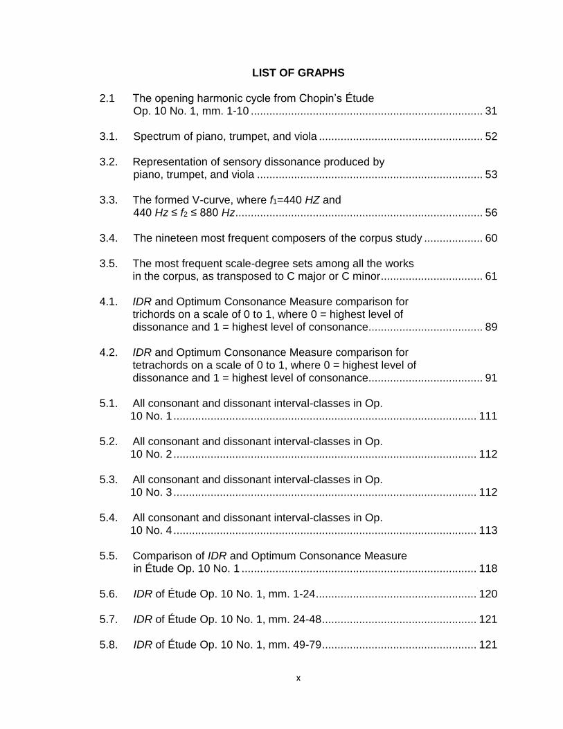
LIST OF GRAPHS

2.1 The opening harmonic cycle from Chopin’s Étude Op. 10 No. 1, mm. 1-10 ........................................................................... 31

3.1. Spectrum of piano, trumpet, and viola ..................................................... 52

3.2. Representation of sensory dissonance produced by piano, trumpet, and viola ......................................................................... 53

3.3. The formed V-curve, where f1=440 HZ and 440 Hz ≤ f2 ≤ 880 Hz ................................................................................ 56

3.4. The nineteen most frequent composers of the corpus study ................... 60

3.5. The most frequent scale-degree sets among all the works in the corpus, as transposed to C major or C minor ................................. 61

4.1. IDR and Optimum Consonance Measure comparison for trichords on a scale of 0 to 1, where 0 = highest level of dissonance and 1 = highest level of consonance..................................... 89

4.2. IDR and Optimum Consonance Measure comparison for tetrachords on a scale of 0 to 1, where 0 = highest level of dissonance and 1 = highest level of consonance..................................... 91

5.1. All consonant and dissonant interval-classes in Op. 10 No. 1 .................................................................................................. 111




5.5. Comparison of IDR and Optimum Consonance Measure in Étude Op. 10 No. 1 ............................................................................ 118

5.6. IDR of Étude Op. 10 No. 1, mm. 1-24 .................................................... 120

5.7. IDR of Étude Op. 10 No. 1, mm. 24-48 .................................................. 121

5.8. IDR of Étude Op. 10 No. 1, mm. 49-79 .................................................. 121

xi

5.9. Combining the IDR and the Optimum Consonance Measure analyses in Étude Op. 10 No. 2 .............................................. 126

5.10. The IDR analysis of all seven phrases in Étude Op. 10 No. 2 with identical opening motive at mm. 1-2 ..................................... 128

5.11. The IDR and the Optimum Consonance Measure analyses of Chopin’s Étude Op. 10 No. 3 .............................................. 130

5.12. The IDR analysis of all phrases in Étude Op. 10 No. 3 .......................... 132

5.13. The IDR and the Optimum Consonance Measure analyses of Chopin’s Étude Op. 10 No. 4 .............................................. 136

xii

ABSTRACT

Chopin’s twenty-seven piano études display the composer’s poetic musical

language, uniting keyboard techniques, virtuosity, and artistic imagery, while

preserving Romantic lyricism and songfulness. Each of these studies is unique in

its set of pianistic challenges, compositional processes, and difficulty level.

Schenkerian analysis provides an interpretation of relationships between the notes

that constitute the harmony and the melody. This type of analysis allows one to

understand the theoretical aspects that are necessary to play Chopin’s études.

The Schenkerian theories can be used to amalgamate pianism and performance

with harmony and analysis. Furthermore, the Schenkerian understanding of these

études provides an analytical dissection of the compositions that can help explain

certain pianistic techniques by the notions of musical elaborations, which include

arpeggiation, as seen in Op. 10 No. 1, chromaticism, as seen in Op. 10 No. 2, and

linear progressions, as seen in Op. 10 Nos. 3 and 4. Throughout these four

compositions, Chopin employs different levels of harmonic dissonance to create

tension and to move between any two harmonic structures.

This study traces the amount of dissonance in each of the études, focusing

on the intervallic makeup of Chopin’s harmonies. The notion of harmonic

dissonance and consonance in music is established from two or more

simultaneously played notes. There are multiple approaches into dissecting this

concept, some of which are acoustical, mathematical, and psychological. This

research uses the Interval Dissonance Rate (IDR) – a tool that integrates musical

and mathematical analyses in non-monophonic Western music, using modified

xiii

interval-class vectors (modicv) and the frequency of recurrent pitches to determine

the percentage of dissonant and consonant verticalities. The connection between

pianism, Schenkerian analysis, and computation of dissonance is a vital aspect to

consider when understanding these études on both artistic and analytical levels.

1

CHAPTER 1. INTRODUCTION

Frédéric Chopin’s works are among the most widely known compositions in

the piano literature of the Romantic period. Chopin is responsible for the output of

over two-hundred pieces of various forms and genres, including four ballades, two

piano concerti, twenty-seven piano études, four scherzi, three sonatas, as well as

multiple mazurkas, nocturnes, polonaises, and waltzes.1 While educated

according to the music traditions of Mozart, Haydn, and Beethoven, Chopin falls

into a unique category of composers who were equally virtuoso pianists, which is

why his music is especially influential to other similar artists, such as Louis

Gottschalk, Henri Herz, Franz Liszt, Anton Rubinstein, Alexander Scriabin, and

Sergei Rachmaninoff.2 Chopin’s life bifurcates between Poland and France, with

1830 being the year of the composer’s immigration, due to the November

Uprising.3

Despite the many changes occurring in his life, Chopin’s style is established

early in his career and does not undergo significant stylistic evolution, even though

some of his later works are more “ambitious” and “audacious.”4 After Chopin’s

1 William A. Palmer, Chopin: An Introduction to his Piano Works (New York, NY: Alfred Publishing, 1971): 2. 2 Jonathan D, Bellman, Chopin and his World (Princeton, NJ: Princeton University Press, 2017), 150-151. Nicholas Cook, "Between Process and Product: Music and/as Performance," Music Theory Online 7, no. 2 (April 2001). Robert Rimm, The Composer-Pianists: Hamelin and the Eight (Portland, OR: Amadeus Press, 2002), 140. 3 Halina Goldberg, The Age of Chopin: Interdisciplinary Inquiries (Bloomington, IN: Indiana University Press, 2004), 8. For more information on Chopin’s nationality and its influence on his music, refer to Richard Taruskin, "Chopin and Gottschalk as Exotics; Orientalism," in Music in the Nineteenth Century: The Oxford History of Western Music. Oxford: Oxford University Press, 2010. 4 Charles Rosen, The Romantic Generation (Cambridge: Harvard University Press, 1998), 360. This is unlike Haydn, Beethoven, and Liszt, who went through major stylistic changes in their compositional careers.

2

immigration to France, the composer continued to produce music inclined by the

Polish character and Polish national traits.5 According to Poniatowska, Chopin is

a “musical poet,” who is “distinct amongst all the great masters of the keyboard

with his artistry being indeterminable in its beauty.”6 While this can be said

regarding multiple genres of works in Chopin’s compositional output, nowhere is

his poetics more evident than in his twenty-seven piano études.7

The purpose of this dissertation is to integrate the artistic and the technical

aspects of pianism and music analysis, based on Schenkerian theories and

theories of consonance and dissonance. For this project, I will be working with

Chopin’s Études Op. 10, Nos. 1-4, using the Interval Dissonance Rate (IDR), an

analytical system that allows one to measure the amount of harmonic dissonance

in a piece of music.8 I will situate my analytical tool in the context of what is already

known about the four études from analytical standpoints.9 Each étude carries its

own set of unique pianistic challenges that a performer must confront. Schenkerian

analysis is a theory that can define and represent these components with notated

elaborations. This dissertation will focus on the integration of Schenkerian studies,

its relation to the pianistic techniques that Chopin presents in each composition,

and how such unity of performance and analysis influences the harmonic

dissonance in these works. The chromatic harmony employed by Chopin in these

5 Irena Poniatowska, Fryderyk Chopin: The Man and his Music (Warsaw: Multico Oficyna Wydawnicza, 2010), 101. 6 Irena Poniatowska, Fryderyk Chopin: A Poet of Sound. 7 These include twelve études in Op. 10, twelve études in Op. 25, and Trois Nouvelles Études. 8 Nikita Mamedov and Robert Peck, “The Interval Dissonance Rate: An Analytical Look into Chromaticism of Chopin’s Op. 10 No. 2 and Scriabin’s Op. 11 No. 2” in Proceedings of Bridges 2017 (Phoenix, AZ: Tessellations Publishing, 2017), 475. 9 These standpoints include Schenkerian analysis, Chopin’s chromatic harmony, and pianism.

3

piano studies likewise impacts the level of harmonic dissonance. Furthermore, this

research will look at methods, in which Chopin utilizes vertical tension, based on

a Schenkerian reading of each work.

There are numerous composers in music history who showcased their

compositional mastery in the creation of études – studies that are meant to perfect

and exercise one or more sets of techniques or musical skills. Nevertheless, the

elements of artistry and lyricism likewise play a crucial role. According to Rosen,

Chopin is the first composer to give piano études a “complete artistic form,” in

which the notions of “musical substance and technical difficulty coincide.”10 Chopin

is one of the most significant composers of études in the Romantic era, providing

innovative pianistic techniques and allowing the performer to enhance his or her

musical abilities and present his or her own interpretation.

In his compositions, Chopin aligns the technical and the lyrical components

of piano performance practice. This is especially evident in his piano études –

exemplary works for analysis when it comes to combining the musical aspects of

technique and artistry. Since the composer employs different levels of harmonic

dissonance throughout his études to move between two or more harmonic

structures, as evident from the analysis of Chopin’s music, his harmonic goals are

not always certain.11 The Schenkerian approach is an example of theory that can

be used to analyze such passages and allows one to trace harmony without

10 Charles Rosen, The Romantic Generation (Cambridge: Harvard University Press, 1998), 363. Chopin is one of the most significant composers of études in the Romantic era, providing innovative pianistic techniques and allowing the performer to enhance his or her musical abilities and present his or her own interpretation. Other notable composers of études are Charles-Valentin Alkan, Claude Debussy, Leopold Godowsky, Franz Liszt, Sergei Rachmaninoff, and Alexander Scriabin. 11 As per Schoenberg, a harmony that has a musical goal and either accepts or rejects the tonic is a chord progression, while a harmony that is aimless is a chord succession.

4

emphasis on Roman numerals, as seen in Der freie Satz, Das Meisterwerk in der

Musik, and Five Graphic Music Analyses.12

A Schenkerian reading can benefit from a quantifying system and the

synthesis of both can be helpful in both performance and analysis.13 From the

perspective of harmonic dissonance, an analyst or a performer can trace the level

of vertical tension among multiple musical passages. When looking at the pianistic

challenges presented by Chopin in his études, it is evident that the first four pieces

of Op. 10 introduce the techniques of playing arpeggios, chromatic scales, and

linear patterns in their purest form.14 Despite these techniques’ being apparent

from the pianist’s point of view, the Schenkerian approach is the most effective

theory to explain the technical aspects that Chopin presents from an analytical

perspective.

The first étude, nicknamed Waterfall, is based on arpeggiation. This work is

composed in the key of C major and contains a strong rhythmic balance with the

bright sounds of the main arpeggiated theme that cover three or four octaves on

every run. Each ascending arpeggio is followed by a descending arpeggio, where

the left hand is generating the bass support. The fluency of the work is derived

through maintaining a steady flow of harmonic tension at its dissonant passages.

The difficulty of this étude lies in the execution of arpeggiated patterns with the

12 Analysis of Tonal Music: A Schenkerian Approach by Cadwallader & Gagné. Introduction to Schenkerian Analysis: Instructor’s Manual by Forte & Gilbert. Unfoldings: Essays in Schenkerian Theory and Analysis by Schachter. These are some of the notable sources on Schenkerian theory. For additional sources on Schenkerian approach to understanding Chopin, refer to the Bibliography section. 13 It is important to note that the theories of Schenker are purely analytical and not quantifiable. On the contrary, many theories of consonance and dissonance employ a computing metric. 14 Regina Smendzianka, How to Play Chopin? Part 3: Chopin's Études.

5

right hand that cover intervals, as large as an eleventh, where an alteration of a

single note can modify the harmony of the composition.15

Furthermore, this étude requires a particular fingering pattern, a strong wrist

control in the right hand, and accurate extensions of the right elbow.16 The fourth

finger is considered as the weakest finger on a pianist's hand according to Chopin's

teaching philosophy, which likewise reflects his compositional approach to writing

for the right hand in the opening étude and therefore, the emphasis of the study on

scales and arpeggios should be directed to the fourth finger.17 Such an approach

to playing arpeggios is the reason why Op. 10 No. 1 is considered as one of the

most difficult pieces of the Op. 10 set.18 In addition, Rosen states that it is possible

to alter Chopin’s fingering pattern to 1-2-5-2, which is particularly advantageous

for the pianists with “moderate sized hands,” yet such a tactic generates issues in

phrasing.19 An excerpt from the opening étude, found in mm. 59-64, can be seen

in Figure 1.1.20

15 An example can be seen in Figure 1.1. Throughout m. 59, the combination of pitches, A, C, and F generate an F major harmony in first inversion. In the first half of m. 60, Chopin preserves notes A and C, yet introduces notes E and F in lieu of pitch F, creating an F♯ seventh chord in first inversion. 16 Charles Rosen, The Romantic Generation (Cambridge: Harvard University Press, 1998), 362. 17 Jon Verbalis, Natural Fingering: A Topographical Approach to Pianism (Oxford: Oxford University Press, 2012), 21. 18 In Op. 10 No. 1, this can be seen in the predominance of 1-2-4-5 fingering pattern on most of the ascending and descending arpeggios. 19 Charles Rosen, The Romantic Generation (Cambridge: Harvard University Press, 1998), 364. 20 Frédéric Chopin, Douze Grandes Études (New York: Schirmer Inc., 1934), 6.

6

Figure 1.1: Chopin’s Étude Op. 10 No. 1, mm. 59-64.

The second étude, nicknamed Chromatique, is based on chromaticism.

This étude is in the key of A minor, where Chopin utilizes ascending and

descending chromatic scales in the right hand, played by the third, fourth, and fifth

fingers, as the main voice varies among multiple triadic chordal structures. This

approach allows Chopin to generate dissonance between the harmonies of the

work, created by the left hand and by the first and the second fingers of the right

hand. An example of this technique can be seen in the first phrase of the étude in

Figure 1.2.21

Like Op. 10 No. 1, a certain fingering pattern must be used for proper

execution throughout majority of the work. Typically, a chromatic scale is played

with the use of the first, second, and third fingers in either right or left hands.22 In

this étude, a pianist must employ the third, fourth, and fifth fingers for the chromatic

21 Ibid., 7. 22 The chromatic scale between two Cs can be played using [1-3-1-3-1-2-3-1-3-1-3-1-2] in the right hand. The chromatic scale between two Cs can be played using [1-3-1-3-2-1-3-1-3-1-3-2-1] in the left hand.

7

ascents and descents, as shown in Figure 1.2.23 Furthermore, the technical

difficulty of this work lies in the generation of clear melody with very little use of

sustaining pedal. Because of constant chromaticism in the right hand, each phrase

generates a sense of a musical curvature, made of ascending and descending

chromatic line, and Chopin makes sure that each arc interacts with the harmony

provided by the left hand and right hand’s inner voices in a unique way.


The third étude, nicknamed Tristesse, is one of the most well-known and

most frequently analyzed studies by Chopin.24 It is based on linear patterns, which

23 This pianistic approach creates difficulties and complexities for pianists in achieving the necessary speed and clarity. 24 Allen Cadwallader and David Gagné, Analysis of Tonal Music. A Schenkerian Approach (New York: Oxford University Press, 2011). Richard Parks, “Voice Leading and Chromatic Harmony in the Music of Chopin,” Journal of Music Theory 20, no. 2 (Autumn 1976): 189-214. Mark J. Spicer, “An Application of Grundgestalt Theory in the Late Chromatic Music of Chopin: A Study of His Last Three Polonaises” PhD diss., University of North Texas. 1994. Mark J. Spicer, “Root Versus Linear Analysis of Chromaticism: A Comparative Study of Selected Excerpts from the Oeuvres of Chopin,” College Music Symposium 36 (1996): 138-147.

8

can be seen in each of the three sections and which occur in both left and right

hands. While Étude No. 1 focuses on large arpeggiated stretches across multiple

octaves and Étude No. 2 concentrates on chromaticism with multiple subordinary

voices, the difficulty of Étude No. 3 lies in the musical contrast of hidden

arpeggiation and chromaticism. This likewise defines the pianistic approach to

performing this work.25 There are three unique characteristics that separate this

étude from the opening two studies of Op. 10.

First, the slow and tranquil tempo of the A-section in the third étude creates

disparity and contrast when compared to the musical characters of Op. 10 Nos. 1

and 2. Furthermore, Chopin generates a distinction between lyricism (as seen in

the A-section of the third étude) and virtuosity (as seen in the étude’s B-section).

Second, Tristesse combines the pianistic concepts of polyphonic voice leading,

cantabile style, and constant legato, all of which integrate to create musical

technical challenges.26 Third, there is an evident dissimilarity in the opening

sections of the third étude, which is seen through tempo, musical character,

harmony, and harmonic dissonance. A passage from Op. 10 No. 3 (mm. 36-44)

can be seen in Figure 1.3.27

25 Kenneth Hamilton, After the Golden Age: Romantic Pianism and Modern Performance (Oxford: Oxford University Press, 2008), 272. 26 Frederick Niecks, Frederick Chopin, as a Man and Musician (London: Novello Inc., 1890), 253. 27 Frédéric Chopin, Douze Grandes Études (New York: Schirmer Inc., 1934), 10.

9


The fourth étude, nicknamed Torrent, is based on linear patterns, in which

a single melody must be executed at a quick tempo against an underlying

harmony.28 This is also the first étude, in which Chopin deliberately alternates the

main melody between the right and the left hands. Unlike Tristesse, this étude is

played in Presto tempo and contains dueling linear patterns between the upper

and the lower voices, which altogether generate perpetuum mobile motion. Like

the third étude, but unlike the first two études, Chopin does not designate

directions for these elaborations and therefore, no patterns to understanding the

motion of the musical motives exist.29

This aspect can be seen in mm. 13-21, shown in Figure 1.4.30 The main

melody can be found in the right hand of mm. 13-16, as the left hand presents

28 Throughout most of Chopin’s études, speed is one of the prominent components that pianists work to excel at. 29 In Op. 10 Nos. 1 and 2, the respective ascending and descending arpeggios and chromatic lines are evident and part of compositional texture. This is not the case in Op. 10 No. 3. 30 Frédéric Chopin, Douze Grandes Études (New York: Schirmer Inc., 1934), 12.

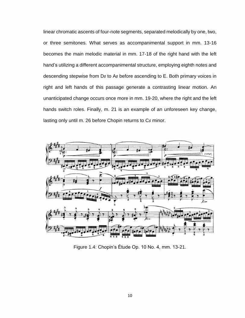
10

linear chromatic ascents of four-note segments, separated melodically by one, two,

or three semitones. What serves as accompanimental support in mm. 13-16

becomes the main melodic material in mm. 17-18 of the right hand with the left

hand’s utilizing a different accompanimental structure, employing eighth notes and

descending stepwise from D♯ to A♯ before ascending to E. Both primary voices in

right and left hands of this passage generate a contrasting linear motion. An

unanticipated change occurs once more in mm. 19-20, where the right and the left

hands switch roles. Finally, m. 21 is an example of an unforeseen key change,

lasting only until m. 26 before Chopin returns to C♯ minor.


11

Dissonance is a prominent component of both music performance and

music theory.31 The study of harmonic dissonance and consonance is derived from

combinations of two or more simultaneously played pitches. The notion of

dissonance has always existed in Western classical music and throughout the

history of music, different composers utilized dissonance in their own unique ways.

Furthermore, composers have individual motivations for the application of

dissonance and in many cases, the tactics for generating multiple levels of

harmonic tension can reveal substantial information regarding the specifics of the

musical style.32

In my dissertation, I will trace Chopin’s use of harmonic dissonance in each

of the opening four études, focusing on the intervallic makeup of their harmonies.

The IDR technique that will be used throughout this dissertation combines the

cognitivist and physicalist approaches to analyzing harmonic verticalities.33 The

IDR will be used to dissect the level of harmonic dissonance from the perspective

of modified interval-class vector, which will be based on eight interval-classes

rather than the traditional six.34 Additionally, I will analyze the dissonance relations

to approaching each work’s culmination points and how such instances of

harmonic tension lead towards the apogees of each étude.

31 Artur Szklener, Chopin in Paris: The 1830s (Warsaw: Narodowy Instytut Fryderyka Chopina, 2006), 245. 32 James Tenney, A History of “Consonance” and “Dissonance” (New York: Excelsior Music Publishing Company, 1988), 42. 33 Ian Cross, “Music Science and Three Views,” Revue Belge de Musicologie / Belgisch Tijdschrift voor Muziekwetenschap 52 (1998): 208. 34 Nikita Mamedov and Robert Peck, “The Interval Dissonance Rate: An Analytical Look into Chromaticism of Chopin’s Op. 10 No. 2 and Scriabin’s Op. 11 No. 2” in Proceedings of Bridges 2017 (Phoenix, AZ: Tessellations Publishing, 2017), 476.

12

There are four parts in this dissertation that follow the Introduction. In the

second chapter, I will discuss the Schenkerian readings of the four études.35 I will

define how the Schenkerian approach combines the notions of pianism and

analysis and how the performance grows out of the background structure.36

Furthermore, I will discuss the chromatic harmony that is found within these works,

how such harmony relates to harmonic dissonance of each étude, and how

Schenkerian analysis allows one to understand and interpret the dissonance from

analytical and interpretational perspectives. I will consider the necessity to highlight

and emphasize harmonic dissonance in Romantic music, as well as its importance

as part of Chopin’s compositional style and its function in each of the four works.

Finally, I will engage with the literature on empirical approaches to idiomatics and

its relation to the introductory four compositions of Op. 10.

In the third chapter, I will cover the main methodologies for working with

dissonance and will discuss the need for incorporating interdisciplinary studies for

accurate analysis.37 I will also define the need for both subjective and objective

dissonance analyses and the necessity for their integration when working with

Western musical repertoire.38 Finally, I will conclude the chapter by discussing the

significance behind quantification methods when analyzing tension in Chopin’s

études.

35 The background and foreground graphs of Op. 10 Nos. 1-4 can be found in the Appendix section of this dissertation. 36 John Rink, The Practice of Performance: Studies in Musical Interpretation (Cambridge: Cambridge University Press, 1995), 108. 37 The interdisciplinary studies covered in this research are music and mathematics, as well as psychology and mathematics. In addition, the literature review can likewise be found in the third chapter. 38 Ian Cross, “Music Science and Three Views,” Revue Belge de Musicologie / Belgisch Tijdschrift voor Muziekwetenschap 52 (1998): 210.

13

The fourth chapter will be dedicated to the description of my analytical tool.

I will explain the main components of the IDR and how such an approach to finding

harmonic dissonance functions in a piece of music. This chapter will likewise

present the mathematical calculations that are necessary to determine the

harmonic dissonance rate and discuss the code that was used for generating the

IDR calculations.39 In addition, the fourth chapter will focus on the perception of

consonance and dissonance from the perspective of meter, define various

rhythmic complexities that arise when using the IDR analysis, and discuss how

these complexities can be resolved.

The fifth chapter will break down the mathematical results retrieved from the

proposed analysis. I will emphasize the data related to harmonic dissonance, its

influence from individual interval-classes, as well as other significant statistical

patterns. Furthermore, I will explain the role that dissonance plays in Chopin’s tonal

ambiguities and how the harmonic dissonance influences the overall structure of

the four pieces examined in this dissertation. Each piece will likewise be dissected

separately and compared with the numerical data retrieved from the Optimum

Consonance Measure analysis – a dissonance metric developed by Huron.40

In the sixth chapter, I will summarize my analytical method, my findings, and

discuss how the knowledge of this information can be used for analysts and

performers alike. I will likewise draw upon the musical connections that exist

39 Nikita Mamedov and Robert Peck, “The Interval Dissonance Rate: An Analytical Look into Chromaticism of Chopin’s Op. 10 No. 2 and Scriabin’s Op. 11 No. 2” in Proceedings of Bridges 2017 (Phoenix, AZ: Tessellations Publishing, 2017), 476. 40 David Huron, “Interval-Class Content in Equally Tempered Pitch-Class Sets: Common Scales Exhibit Optimum Tonal Consonance,” Music Perception 11, no. 3 (Spring 1994): 293.

14

among the data provided by the IDR, the Schenkerian interpretations of each work,

and the performance practice. I will, in addition, propose future research that can

be conducted with this study.

15

CHAPTER 2. PIANISM AND SCHENKERIAN APPROACH

2.1 Pianism and Influence

Music history plays a prominent role in the study of Chopin’s études. One of the

key innovations in the Romantic era is the rise of compositions written particularly

for the improvement of performer’s technique.41 Chopin is one of the significant

composers to focus on this genre and his artistic output is derived from

compositional languages of his predecessors. Therefore, to fully understand

Chopin’s compositional strategies, the works of other composers who influenced

him need to be considered.

Chopin's Op. 10, Op. 25, and Trois Nouvelles Études form the foundation

and the basis for technique and artistry in the piano literature of the Romantic

tradition. In Chopin’s earliest efforts at composing in this genre, the twelve pieces

of Op. 10 encompass some of the most challenging and picturesque music, filled

with poetic symbolism.42 These works are likewise considered as some of the most

popular compositions in modern pianist’s concert repertoire and are frequently

performed in recitals, festivals, and competitions. The musical characterizations

that Op. 10 carries led to the drastic increase of appreciation and appearance of

these works in the concert halls. In addition to the main goal of each composition

to create a fixed musical training based on a specific technique, each of the pieces

likewise provides a musical story, which is why Chopin’s études are considered as

concert works rather than candid technical exercises. Guided by the compositional

41 For more information, refer to: Tim Fulford, Literature, Science and Exploration in the Romantic Era: Bodies of Knowledge (Cambridge: Cambridge University Press, 2007). 42 Franciszek German, "Chopin and Mickiewicz," Rocznik Chopinowski 1 (1956): 235.

16

approaches of his predecessors, Chopin marks the new era in the history of

études, offering innovation to performance practice.43

The works in Op. 10 are essential for professional concert artists from the

perspective of pianism. These twelve short pieces allow one to tackle most of the

major aspect of pianistic techniques. Throughout the history of piano performance

practice, there have been multiple excellent interpretations of these works, each

artistic in own way and each emphasizing on unique musical components. These

include prewar recordings by Vladimir de Pachmann (1927) and Ignacy Jan

Paderewski (1928), as well as postwar recordings by Sviatoslav Richter (1967,

1971, 1976), Maurizio Pollini (1985), Boris Berezovsky (1991), and Lang Lang

(2012).44

Chopin’s compositional techniques in writing in this genre can be traced to

composers of the previous generation, dating back to the early 19th century. Just

like Chopin, early composers of études were interested in piano pedagogy, rather

than refined expertise and virtuosity. Muzio Clementi (1752-1832) is one of the first

such composers who took strides in developing works for enhancing keyboard

techniques. This can be seen in his Gradus ad Parnassum – a set of one-hundred

études, composed between 1817 and 1826.45 Although Clementi’s études are

43 Frederick Chopin and Albert R. Parsons (ed.), Frederick Chopin's Works: Instructive Edition with Explanatory Remarks and Fingerings by Dr. Theodore Kullak (New York: Schirmer, 1880), 1. 44 Sviatoslav Richter, Richter Plays Chopin, Melodiya 10-01626, 2012. Maurizio Pollini, Chopin Études, Deutsche Grammophon 00289-477-8423, 1985. Boris Berezovsky, Chopin Études, Teldec 9031-73129-2, 1991. Lang Lang, The Chopin Album, Sony Classical 88725449602, 2012. 45 Muzio Clementi, Gradus ad Parnassum (New York: Schirmer, 1908), 7. The first book contains Études Nos. 1-27; the second book contains Études 28-50; the third book contains Études Nos. 51-100.

17

highly repetitive in its motivic content, they are technical and challenging, when

compared to compositions of his era.

In some of the études, Clementi provides more than one possible set of

fingerings in which a technical challenge can be executed. Figure 2.1 shows mm.

1-4 of Étude No. 2, where Clementi presents the performer with three different

fingering variations.46 As seen from the example, the main melody is presented in

the right hand, while the technical aspect of this étude is presented in the left hand

and is based on variations of a stepwise ascending and descending motive.

Figure 2.1: Clementi’s Étude No. 2, mm. 1-4.

Chopin's rejection of the standard fingering technique in piano literature is

widely known and in his études, Chopin develops own fingering patterns, based

on the technical challenges imposed on the pianist.47 Similar to the Clementi’s

46 Ibid., 7. 47 Jon Verbalis, Natural Fingering: A Topographical Approach to Pianism (Oxford: Oxford University Press, 2012), 72. Chopin's approach to determining the fingerings allow for more consistency, elegancy, and smoothness, when moving across the keyboard. The fingering provided in Chopin's études transformed the pianist's approach to studying Romantic repertoire.

18

example, Chopin’s Op. 10 No. 1 is a technical study, where the composer presents

passages that can be played in more than one way. This can be seen in m. 28 and

m. 30, shown in Figure 2.2, where the descending melody can be performed with

two sets of fingerings.48 The fingering patterns that pianists apply are determined

by multiple factors, such as speed, voicing, technique, and rhythm.49 The emphasis

on fingering allows for various interpretations in performance practice, which

include phrasing, dynamics, articulation, and memorization.50


English pianist and composer Johann Baptist Cramer (1771-1858) writes

Studio per il Pianoforte – a set of 84 études between 1804 and 1808.51 It is

48 Frederick Chopin and Albert R. Parsons (ed.), Frederick Chopin's Works: Instructive Edition with Explanatory Remarks and Fingerings by Dr. Theodore Kullak (New York: Schirmer, 1880), 3. In m. 28, a pianist may choose either a 5-3-2-1 pattern on all four descending arpeggios or 5-2-1-3 on the first three arpeggios with the return of 5-3-2-1 on the last set to prepare for m. 29. A similar concept can be traced in m. 30, only the primary fingering choice is 5-4-2-1 because of the three

black keys (E♭, B♭, and E♭) in each arpeggio. 49 Richard Parncutt, John A. Sloboda, Eric F. Clarke, Matti Raekallio, and Peter Desain, “An Ergonomic Model of Keyboard Fingering for Melodic Fragments,” Music Perception 14 no. 4 (Summer 1997): 341. 50 Ibid., 342. Parncutt et al. argue that one’s interpretation and the quality of one’s playing depends on the set of fingering that a pianist chooses. Furthermore, Parncutt et al. developed a model to predict the best recommended fingering pattern in performance, which depends on the degree of comfortability. A modified version of the system was presented by J. Pieter Jacobs. 51 Johann Baptist Cramer, Studio per il Pianoforte (Leipzig: C. F. Peters, 1890): 1-168. The first book of 42 études was completed in 1804 and the second book of 42 études was completed between 1807 and 1808.

19

unknown, yet possible that Chopin was aware of Cramer’s piano studies, since

there are a few resemblances in the compositional style of both composers. Figure

2.3 shows the opening two bars of Cramer's Étude No. 1. After the initial C major

chord, Cramer continues with an ascending motivic structure moving in parallel

motion in both hands. In Op. 10 No. 4, Chopin begins in similar fashion, only with

a motivic ascent in the right hand in m. 1 and a motivic descent in the right hand in

m. 2, shown in Figure 2.4.52 Figure 2.5 presents the same phrase in the left hand,

repeated in mm. 5-6.

Figure 2.3: Cramer’s Étude No. 1, mm. 1-2.


52 Frédéric Chopin, Douze Grandes Études (New York: Schirmer Inc., 1934), 14-18.

20


Carl Czerny (1791-1857), one of the most prolific composers and

pedagogues in the history of Western music with over a thousand completed

works, is one of the most significant early composer of piano études and has

influenced Chopin in his works. Having taught some of the greatest piano

technicians of the Romantic era, such as Franz Liszt, Theodor Leschetizky, and

Theodor Kullak, Czerny completed multiple sets of technical studies, all of which

vary in form, speed, technique, and difficulty level. An influence of Czerny’s Op.

740 No. 12 can be seen in Chopin’s Op. 10 No. 12. In Czerny’s work, mm. 7-8

serve as transition to return to the reinstatement of the main theme, where the left

hand contains a stepwise descent, interrupted by a static repetition of pitch A, as

seen in Figure 2.6.53 A similar pattern exists in mm. 25-27 of Chopin’s Op. 10 No.

12, only the left hand contains a stepwise ascent from pitch D to G♭ with a static

repetition of B♭-C♭-B♭ in bar 25 and B♭-C♮-B♭ in bar 26, as seen in Figure 2.7.

53 Carl Czerny, Die Kunst Der Fingerfertigkeit (Frankfurt: C. F. Peters, 1950), 42.

21

Figure 2.6: Czerny’s Étude Op. 740 No. 12, mm. 7-8.


The closest precursor to Chopin’s études is the compositional output of

Maria Szymanowska (1789-1831), known for her Vingt Exercises et Préludes,

completed in 1820.54 Szymanowska is the first Polish-born composer to write a set

of études.55 At the time when Chopin was attending the Warsaw Conservatory,

Szymanowska already established her career as a composer and a pianist.56

Throughout the research of Polish music, there have been a lot of parallels drawn

between both composers. For instance, it is a known fact that both artists knew

54 Zofia Chechlińska. "Szymanowska, Maria Agata." Oxford Music Online, accessed January 12, 2018, http://www.oxfordmusiconline.com/subscriber/article/grove/music/27327. 55 Irena Poniatowska, Historia i interpretacja muzyki. Z badań nad muzykš od XVII do XVIII wieku (Warsaw: Musica Iagellonica, 1995), 95. 56 Slawomir Dobrzański, “Maria Szymanowska and Fryderyk Chopin: Parallelism and Influence,” Polish Music Journal 5, no. 1 (Summer 2002): 1

22

each other and were aware of the similarities in their compositional careers.57

Furthermore, amalgamated by similar Polish traditions and driven by the notions

of Polish nationalism, some of the genres in which Szymanowska composed align

with Chopin’s compositional output and include études, mazurkas, nocturnes,

polonaises, preludes, and waltzes.58 While Chopin never discussed or mentioned

Szymanowska’s effect on his music, her influence on his works is non-debatable.59

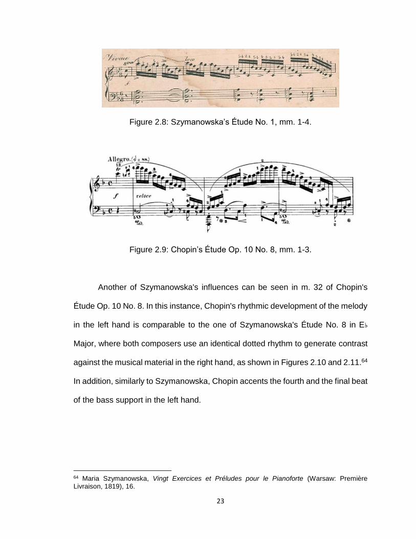
Szymanowska's harmonic models and approaches to melodic

developments have served as examples for Chopin's études.60 In her Étude No. 1

in F major, Szymanowska begins with an anacrusis on note C that leads to a series

of sixteenth notes in the right hand of the main melody, supported by the bass

structure in the left hand, as seen in Figure 2.8.61 Chopin begins his Étude Op. 10

No. 8 in a similar manner with an anacrusis starting on pitch C, initializing the main

melody with a technical passage in the right hand, accompanied by the steady

supporting line in the left hand, as seen in Figure 2.9.62 Furthermore, the spacing

on the downbeat between both hands is identical and the musical material, found

in the right hand of both études, contains an evenly spaced melody of a broken

chordal figuration of F major tonic.63

57 Ibid., 25. 58 Mieczysław Tomaszewski, Chopin: Człowiek, Dzieło, Rezonans (Poznań: Podsiedlik, 1998), 588. 59 Stefania Łobaczewska, Z dziejów polskiej kultury muzycznej (Kraków: PWM, 1966), 157. 60 Halina Goldberg, Music in Chopin's Warsaw (Oxford: Oxford University Press, 2008), 194. 61 Maria Szymanowska, Vingt Exercices et Préludes pour le Pianoforte (Warsaw: Première Livraison, 1819), 2. 62 Frédéric Chopin, Douze Grandes Études (New York: Schirmer Inc., 1934), 24. 63 Sławomir Dobrzański, “Maria Szymanowska and Fryderyk Chopin: Parallelism and Influence”, Polish Music Journal 5, no. 1 (Summer 2002): 10.

23

Figure 2.8: Szymanowska’s Étude No. 1, mm. 1-4.


Another of Szymanowska's influences can be seen in m. 32 of Chopin's

Étude Op. 10 No. 8. In this instance, Chopin's rhythmic development of the melody

in the left hand is comparable to the one of Szymanowska's Étude No. 8 in E♭

Major, where both composers use an identical dotted rhythm to generate contrast

against the musical material in the right hand, as shown in Figures 2.10 and 2.11.64

In addition, similarly to Szymanowska, Chopin accents the fourth and the final beat

of the bass support in the left hand.

64 Maria Szymanowska, Vingt Exercices et Préludes pour le Pianoforte (Warsaw: Première Livraison, 1819), 16.

24

Figure 2.10: Chopin’s Étude Op. 10 No. 8, m. 32.

Figure 2.11: Szymanowska’s Étude No. 8, mm 1-4.

The composers, mentioned above, have added substantially to this genre,

yet it was Chopin, who established the étude as a concert work, rather than a mere

pedagogical exercise. While unique in ternary form, the twelve études of Op. 10

are all diverse in the level of difficulty. For instance, Études No. 3 in E Major and

No. 6 in G♭ Minor are among the easier studies of the set. According to Robert

Schumann, both études lack technical challenges related to speed, yet present

musical artistry, where a pianist needs to have excellent control of melody and

accompaniment with one hand at the same time.65 On the contrary, Études No. 1

in C Major, No. 2 in A Minor, and No. 4 in C♯ Minor, are among some of the most

difficulty studies of the set and as the level of artistry and technique among

65 Robert Schumann, "Die Pianoforte-Etuden, ihren Zwecken nach geordnet," Neue Zeitschrift für Musik 11 (February 6, 1836), 46.

25

professional pianists increased, these études were becoming essential for

performers in order to improve their technical abilities. Throughout his

compositional career, Chopin created his own unique musical style and while

influenced by composers of previous generations, Chopin’s études present

fundamental pianistic techniques in unique and innovative ways.

Finally, it is important to note that Chopin’s études have influenced

composers of subsequent generations.66 For instance, Chopin’s Op. 10 and Op.

25 have carved the way for Alexander Scriabin’s set of twelve Op. 8 études,

composed in 1894. Scriabin’s early études are based on the Chopinesque style,

form, as well as melodic and accompanimental presentations.67 Figures 2.12 and

2.13 show the influence of Chopin’s Op. 25 No. 8 in D♭ Major on Scriabin’s Op. 8

No. 6 in A Major. Both études are based on the intervals of major and minor sixths,

seen in right and left hands. In the right hand, these intervals function as a double

primary melody, while in the left hand, these intervals are used for the purpose of

accompaniment. Such texture in both works stays consistent until the very last

measure. This example shows that Scriabin deliberately followed Chopin’s

compositional approach.68

66 Irena Poniatowska, Fryderyk Chopin: The Man and his Music (Warsaw: Multico Oficyna Wydawnicza, 2010), 101 67 Stephen Downes, Music and Decadence in European Modernism: The Case of Central and Eastern Europe (Cambridge: Cambridge University Press, 2010), 226-227. Daniel Dewitt Mickey, “An Analysis of Texture in Selected Piano Études of Chopin and Scriabin,” (Master's Thesis, Ohio State University, 1980), 8. 68 Yuri Bortz, “The Stylistic Foundation in the Etudes of Chopin, Scriabin, and Messiaen,” Master’s Thesis, University of Akron, 1997.

26

Figure 2.12: Chopin’s Étude Op. 25 No. 8, mm. 1-2.69

Figure 2.13: Scriabin’s Étude Op. 8 No. 6, mm. 1-3.70

Another Polish composer and pianist who was influenced by Chopin’s

études is Leopold Godowsky (1870-1938). He is most known for his Studies on

Chopin's Études – a set of fifty-three arrangements, based on Chopin's Opp. 10,

25, and Trois Nouvelles Études, completed between 1894 and 1914.71 These

compositions are considered as some of the most difficult and technical piano

works in the literature, where Godowsky implements extra technical challenges on

top of the already existing ones from Chopin's études.72 Despite the difficulty level,

69 Frédéric Chopin, Études Op. 25 (Leipzig: C. F. Peters, 1879), 28. 70 Alexander Scriabin, The Complete Preludes & Études for Pianoforte Solo (New York: Dover Publications, 1973), 170. 71 Charles Hopkins. "Godowsky, Leopold." Oxford Music Online, accessed December 15, 2017, http://www.oxfordmusiconline.com/subscriber/article/grove/music/11344. 72 Harold Schonberg noted that Godowky’s études push the piano technique to its maximum limits. Robert Rimm, The Composer-Pianists: Hamelin and the Eight (Portland, OR: Amadeus Press, 2002), 242.

27

Godowsky’s études clearly present his pedagogical philosophy at the keyboard,

amalgamating mechanical, technical, and musical aspects of piano playing. Figure

2.14 shows mm. 25-26 of Chopin’s Op. 10 No. 1, where the phrase begins with a

broken ascending and descending arpeggiated sequence in the right hand. Figure

2.15 shows mm. 25-26 of Godowsky’s transcription of the same étude, where the

technique of playing broken arpeggios must be executed in both hands in contrary

motion.73

Figure 2.14: Chopin’s Étude Op. 10 No 1, mm. 25-26.

Figure 2.15: Godowsky’s Étude No. 1, mm. 25-26.

73 Leopold Godowsky, Studien über die Etüden von Chopin (Berlin: Schlesinger, 1914), 5.

28

The various aspects of pianism are significant from the perspective of

Schenkerian analysis. A composition’s pianism is seen in the musical path that a

composer chooses for harmony and melody. Schenkerian analysis dissects such

a path and presents analytical observations and hierarchical relationships between

the prominent pitches located in the score. Furthermore, Schenkerian analysis

allows one to view a composition by focusing on multiple musical layers, each

consisting of its own analytical details. Schenkerian analysis additionally portrays

the directions and the relations between the elements provided by pianism and

reflects many musical nuances from the composer's perspective. While the

performance of a composition grows out of the background structure in

Schenkerian analysis, it is nevertheless possible to apply such theory to graph the

performer’s interpretations. According to Schenker, the performance of a musical

work is based on one's perception and one’s musical understanding and therefore,

"musical punctuations" that a pianist provides in a work’s motives, themes, and

phrases can be reflected via the means of a Schenkerian representation.74

2.2. The Schenkerian Approach, Op. 10 No. 1

The principles of Schenkerian analysis explain the structure of a musical work by

employing the technique of prolongation. Schenkerian prolongations consist of

various elaborations that allow one to connect the work through multiple linear

units. Prolongation in Schenkerian analysis explains the development and the

expansion of all melodies and harmonies throughout a composition. In addition,

74 Heinrich Schenker, Der Freie Satz, Volume III (New York: Longman, 1935), 8.

29

understanding prolongation allows one to understand the basics of artistic

consistency in performance.

Previous research history of Chopin’s music shows that there exist

theoretical tools that help explain the composer’s analytical intentions and the

analysis of Chopin’s music can be understood through the artistic meaning that the

composer embodies in each of his works. For instance, Schenkerian theory is an

appropriate approach that combines pianism and harmony, and explains the

technical aspects that Chopin presents in his études. This occurs from the

standpoint of three Schenkerian elaborations: arpeggiation, as seen in Étude No.

1, chromaticism, as seen in Étude No. 2, and linear patterns, as seen in Études

Nos. 3 and 4. Schenkerian analysis allows one to dissect Chopin’s harmonic

language and trace the pianistic proficiency that is expected of the performers.

Charles Rosen combines the notions of pianism with analysis in his book

The Romantic Generation (1998). According to Rosen, Étude Op. 10 No. 1 is a

prime example of a work, in which a change of harmony is evident and is based

on phrasing of the broken ascending and descending arpeggios.75 The musical

idea that Chopin presents is realized through the physical configuration of hand

and arm. Therefore, the unification of the technique with musical thought generates

a unique pianistic style of this étude. While the arpeggiated patterns continue

75 Charles Rosen, The Romantic Generation (Cambridge, MA: Harvard University Press, 1998), 364.

30

throughout the whole work, it is the harmonic reduction that allows one to notice

the shape, the structure, and the curvature of the composition.76

Figure 2.16 shows the harmonic reduction of mm. 1-10 of the étude,

encompassing the first phrase and the opening two bars of the second phrase, as

seen in Czerny’s School of Practical Composition (1840).77

Figure 2.16: Harmonic reduction of Chopin’s Étude Op. 10 No. 1, mm. 1-10.

Graph 2.1 illustrates the alterations of harmonies in the opening cycle.78

Chopin initializes and finalizes this cycle in an identical manner through the means

of C major tonality in mm. 1-2 and mm. 9-10. The other harmonies presented in

this cycle are F major in m. 3, F♯ diminished seventh in m. 4, G major in m. 5, D

dominant seventh in m. 6, and G dominant seventh in mm. 7-8.79 The tonic C

76 Harmonic reduction is the initial step taken in the generation of Schenkerian analyses. The harmonic reduction (chordal configuration) leads towards the creation of the imaginary continuo, which leads towards the generation of the Schenkerian graphs. Allen Cadwallader and David Gagné, Analysis of Tonal Music: A Schenkerian Approach (Oxford: Oxford University Press, 2011), 66. 77 Carl Czerny, School of Practical Composition, Volume I (London: Robert Cocks & Co., 1848), 92. 78 The first phrase of Op. 10 No. 1 is found in bars 1-8; the second phrase of the A-section is initialized in mm. 9-10. Cohn’s term closed harmonic cycle can be used to define mm. 1-10. According to Cohn, the harmonies of a passage form a cycle if such a passage incorporates an ordered set of at least four elements, where the first and the last elements are identical, while the other elements are distinct. The first cycle of Op. 10 No. 1 contains six unique elements. Richard Cohn, “Maximally Smooth Cycles, Hexatonic Systems, and the Analysis of Late-Romantic Triadic Progressions,” Music Analysis 15, no. 1 (March 1996), 15. 79 Abbreviations used: M = major; m = minor; dim = diminished; 7 = seventh chord.

31

major, the subdominant F major, and the dominant G major are the three

harmonies in the cycle shown in their pure triadic structure, where Chopin only

incorporates the root, the third, and the fifth.

Graph 2.1: The opening harmonic cycle from Chopin’s Étude Op. 10 No. 1, mm. 1-10.

Schenkerian analysis shows that Op. 10 No. 1 is built entirely on chords

that form combinations of rhythmically defined phrases in each of the three

sections. According to Czerny, Chopin makes sure that each chord receives an

appropriate musical answer, essential to sustain the melodic idea of the étude.80

Even though Op. 10 No. 1 is based solely on arpeggiation, this is an example of

Chopin’s use of “real melody” rather than “accidental melody.”81

Rosen states that the theoretical notions of the work, seen in the phrasing

through the arpeggios, can be amalgamated with Chopin’s intended pianistic

technique. Musical interpretation can be reflected through Schenkerian analysis,

80 Carl Czerny, School of Practical Composition, Volume I (London: Robert Cocks & Co., 1848), 93. 81 Ibid., 94. Real melody stays the same even without any accompaniment. The real melody is still “intelligible”, “full of meaning”, and is “capable of being sung”. Accidental melody is the type of melody that needs an accompaniment to be recognized.

32

which is the approach taken by Rosen to combine both theoretical and pianistic

concepts of Op. 10 No. 1. The hand and the arm configurations about which Rosen

writes are marked with arrows, representing the alternating ascending and

descending arpeggio patterns. Each of the patterns is a Schenkerian arpeggiated

elaboration, signified by a group of two slurred quarter notes, seen in the first

phrase of Figure 2.17. This Schenkerian understanding of the passage likewise

reveals the musical characterization that a pianist depicts in a performance.

Figure 2.17: The hand-arm motion effect from perspective of the Schenkerian analysis, seen in Chopin’s Étude Op. 10 No. 1, mm. 1-10.

Appendix 1 presents the background Schenkerian analysis of Op. 10 No. 1.

The background graph of the work allows one to trace the form, the structure, and

the central harmonic structure of the composition. The Ursatz of the étude consists

of fundamental ^3-^2-//-^3-^2-^1 Urlinie with an interruption (labeled as //)

occurring at the end of the B-section before the reinstatement of A at m. 49. The

33

interruption separates sections A and B from A; while both A and B sections are

twenty-four bars in length, section A consists of thirty-one bars. The symmetry in

the measure length found in the opening forty-eight bars of the étude reveals

Chopin’s intent to create a musical equilibrium between the opening two sections.

Appendix 2 presents the foreground Schenkerian graph of Op. 10 No. 1.

Based on the foreground graph, it is evident that the identical pianistic technique

is used throughout the piece and every two-measure unit incorporates the

arpeggiation elaboration. The graph reveals that, while a variety of harmonies exist

in the A-section, the highest pitch that Chopin includes in the right hand of the

étude is ^3. In fact, the only three pitches used as the apogee of every arpeggiation

pattern are D, D♯, and E (^2, ^♯2, and ^3). From the perspective of form, each of

the composition’s three eight-measure phrases is generated by these two-

measure units.82

In the B-section, Chopin’s compositional approach to treating the apogee of

each arpeggiation changes, as the composer utilizes a greater variety of pitches

and harmonic regions. A unique choice of harmony to generate a cadential ending

can be observed in mm. 23-24, where Chopin utilizes the E major mediant instead

of the G major dominant, leading the B-section to begin with a resolution into A

major harmony.83 A similar occurrence happens in mm. 47-48 at the end of the B-

section. This time, however, the E major transforms into G7 before returning to C

major tonic in section A at m. 49. Another significant aspect of the B-section is its

82 Such symmetry is interrupted in the final section of the étude. 83 Beethoven uses this technique in his Piano Sonata No. 21, Op. 53, where the opening theme in C major modulates to E major, the key of the secondary theme in the first movement. Ludvig Van Beethoven, Klaviersonaten (Munich: G. Henle Verlag, 1980), 88.

34

use of linear sequences in the bass of the left hand to lead a series of ascending

and descending arpeggios in the right hand. This can be observed in three

instances: two passages in mm. 25-33 and mm. 42-47, both containing the

sequential descent of melodic perfect fourths, and one passage in mm. 35-41 that

incorporates the sequential descent of melodic perfect fifths.84


Structurally, the second étude is similar to Op. 10 No. 1.85 While the technical

challenges vary, the pianistic aspects of legato, accuracy, and voicing should still

be implemented by the performer. Unlike the first étude, the main pianistic purpose

of Op. 10 No. 2 is to achieve evenness, consistency, and strength in the right

hand's three weakest fingers. Chopin uses very little innovation in this work,

focusing on the chromaticism in the right hand and chordal harmony in the left

hand, as well as in the secondary voices of the right hand.

Chopin’s ability to expand thematic material is evident in mm. 13-16, where

an ascending chromatic run from A to F in mm. 13-14 develops and transforms

into an ascending chromatic run from B♭ to A♮ in mm. 15-16, as shown in Figure

2.18. On the first chromatic rise, Chopin begins with a tonic harmony, moves

towards the subdominant harmony, and returns to the tonic harmony, which

generates an A minor D minor A minor progression. Chopin initializes the

84 Bars 25-33 (movement by fourths): (A-D) (G-C) (F-B♭);

Bars 42-47 (movement by fourths): (E-A) (D-G) (C-F) (B-E);

Bars 35-41 (movement by fifths): (A-D) (G-C) (F-B♭). 85 Furthermore, the directions of Schenkerian elaborations are likewise evident throughout the second étude.

35

second chromatic ascent with the Neapolitan harmony before moving to the

dominant harmony. Instead of returning to the tonic, Chopin finalizes the musical

apex with the submediant harmony, which generates a B♭ major E dominant

seventh F major progression. The common characteristic of mm. 13-14 and

mm. 15-16 is the ascending and descending primary chromatic melody, yet Chopin

utilizes diverse harmonic paths and stresses different metric spots for the pitch

zeniths. The highest pitch in the initial ascent occurs on the first (strong) sixteenth

note of the second beat. On the contrary, the highest pitch in mm. 15-16 ensues

on the last (weak) sixteenth note of the fourth beat in m. 15.


Appendix 3 presents the background Schenkerian analysis of Op. 10 No. 2.

The background graph reveals the untraditional path of the Urlinie throughout the

work. First, this is the first example of ^5-^1 line in the Op. 10 set. Second, the

Urlinie occurs three times in the étude, each time amalgamating new melodic and

harmonic material. Third, the descent of the Urlinie in each of the final two

36

instances is based on a harmonic minor scale with a raised ^7, since A is followed

by G♯, not a G♮. Fourth, this is the only one of Chopin’s études to end on a Picardy

third, where the final note of the melody is found in the right hand and ends on C♯

rather than C♮. According to Schenker, the goal of the fundamental structure is to

“represent tonality” and to “achieve musical coherence” through the means of

stepwise descent from either ^8, ^5, or ^3.86 Even though ^1 is the final stated goal,

it is achieved in m. 45 with mm. 45-49 serving as post-cadential closure, which

includes an ascending chromatic rise and a descending chromatic return to the

Picard third.87

Appendix 4 presents the foreground Schenkerian graph of Op. 10 No. 2.

Based on the foreground graph, it is evident that the main thematic passage in

mm. 1-2 (mot. a1) generates the melodic and harmonic expansion of each of the

four phrases in Section A.88 The opening two measures are identical to mm. 5-6

(mot. a2), mm. 9-10 (mot. a3), and mm. 13-14 (mot. a4). Each of these musical

statements introduce a short phrase. A similar idea applies to section A, where

mm. 1-2 are identical to mm. 36-37 (mot. a5), mm. 40-41 (mot. a6), and mm. 45-46

(mot. a7). The final three motives are responsible for all three phases in the final

section of the étude. Based on the homogenous structure of the piece, the

86 Heinrich Schenker, Der Freie Satz, Volume III (New York: Longman, 1935), 5-6. 87 It is important to mention that it is likewise possible for the Schenkerian Urlinie to fail reaching ^1, an example of which is presented Marston's Schenkerian graph of Schumann's Kinderszenen Op. 15 No. 1, where the Urlinie closes on ^3. Nicholas Marston, Heinrich Schenker and Beethoven's Hammerklavier' Sonata (London: Ashgate Publishing, 2013), 90. 88 The key characteristic of Op. 10 No. 2 is that Chopin initializes multiple phrases in an identical manner. In this section, each such initialization will be labeled as mot. ax. Therefore, mm. 1-2 = mot. a1; mm. 5-6 = mot. a2; and so on. Since all mot. ax share identical music material, it is to the benefit of a pianist to create artistic disparity in the way these motives are performed and the changes in performance practice can be traced through the use of Schenkerian analysis.

37

analytical representation of similarity at the beginning of each phrase is significant

from the perspective of performer, since an identical playing of these motives is

not encouraged. Therefore, a performer needs to decide on specific artistic

characteristics that can enhance this work musically.

Figure 2.19: Schenkerian representation of Shishkin’s performance of Op. 10 No 2, mm. 1-16.

38

This can be seen and analyzed in Dmitry Shishkin’s performance of Étude

Op. 10 No. 2 at the 17th International Fryderyk Chopin Piano Competition.89 Figure

2.19 shows the foreground graph of Shishkin’s interpretation of section A. In mot.

a1, there is a slight accent on note A in the left hand of the first beat on bar 2. As

evident from the foreground graph, the pitch A is prolonged in mm. 1-2 and

therefore, an identical note is not needed. Figure 2.19 likewise reveals that the

primary prolonged pitch A is interconnected with a supplementary pitch A (as a

quarter note), which Shishkin accents with the use of a dotted slur. Therefore, while

the A minor harmony is prolonged, it is also emphasized.

In mot. a2, no evident interpretational changes exist, although there is an

emphasis on note E in the left hand of the second beat on m. 8. As in the previous

example, no additional pitch E is necessary, since the E on the first beat of m. 8

represents the prolonged dominant harmony for the full bar. However, Shishkin’s

interpretation requires an additional quarter note E on the second beat to

emphasize the harmony.

The mot. a3 contains a similar execution as mot. a1, except the accent on

note A in the left hand of the first beat on m. 2 is stronger and more apparent. The

Schenkerian analysis represents this by using a half note to define the additional

note A, instead of a quarter note, as it was done in mot. a1. Furthermore, Shishkin

brings out the pitches D♯ and E of the secondary melody in the middle voices of

the right hand, found on the second and third beat of m. 12. Since this does not

happen in mot. a1, the pitches D♯ and E (of mot. a3) are represented as individual

89 Dmitry Shishkin, Chopin. Études, Polonaise in A-flat Major Op. 53, Scherzo in B-flat Minor Op. 31 Fryderyk Chopin Institute B01LWQ527E, 2016.

39

quarter notes. Finally, mot. a4 has no evident interpretational changes, but the

continuation of mot. a4 in mm. 15-17 incorporates a larger use of sustained pedal.

Additionally, Shishkin creates a slight ritardando before the entrance into the B-

section.

Each interpretation is unique and each pianist’s musical comprehension of

a work can be represented by a distinctive Schenkerian depiction. The musical

components that are idiosyncratic in each performance are based on accentuation

and musical emphasis. Therefore, a series of dynamic accents can be highlighted

by Schenkerian notation, such as filled in noteheads, quarter notes, and half notes.

On the contrary, there are component of performance that Schenkerian analysis

cannot graph. Examples of such components are purely interpretive, such as

tempo alterations and pedaling.


Of the opening four works, the third étude has received the most research and

thorough analysis with notable theoretical studies by Spicer and Parks.90

Cadwallader and Gagné focus on the notion of melody and provide an analytical

interpretation of the opening five measures in Op. 10 No. 3, as seen in Figure

2.20.91 The initial phrase of this composition allows one to outline the arch, where

the tonic pitch E on the first beat of m. 1 ascends to the second scale degree (F♯)

90 Richard Parks, “Voice Leading and Chromatic Harmony in the Music of Chopin,” Journal of Music Theory 20, no. 2 (Autumn 1976): 189-214. Mark J Spicer, “Root Versus Linear Analysis of Chromaticism: A Comparative Study of Selected Excerpts from the Oeuvres of Chopin,” College Music Symposium 36 (1996): 138-147. 91 Allen Cadwallader and David Gagné, Analysis of Tonal Music: A Schenkerian Approach (Oxford: Oxford University Press, 2011), 18.

40

on the second beat of the same measure and to the third scale degree (G♯) on the

second beat of m. 2.


The apogee of the arch descends from G♯ back to tonic in mm. 4-5. The

third measure contains a musical break between the two G♯ of the melodic arch,

revealing the real apex of the phrase – the C♯ on the second beat of m. 3 preceded

by the interval of a perfect fourth. The significance of m. 3 lies in its generation of

dissonance on the dominant harmony that is resolved on the descent towards the

E in m. 5. The tones E, F♯, and G♯ are heard as primary elements of the main

melody of the étude.92

The harmonic reduction of this passage reveals the Chopinesque melodic

arch in its highest voice, supported by the tonic on the first and the third scale

degrees, and by the dominant on the second scale degree.93 Furthermore, the

inclusion of pitch B in the pickup measure fulfills the outline the tonic triad through

the means of “continuity” and “variety.”94 The consistence of lyrical and melodious

92 Ibid., 17. 93 The complete background and foreground graphs of Étude Op. 10 No. 3 can be viewed in Appendices 5 and 6. 94 Ibid., 18.

41

qualities that Chopin presents in the third étude is the technical challenge in itself,

seen in the analytical interpretation and the chordal configuration of the opening

phrase. This instance of Chopin’s melodic development illustrates the meaning of

the analysis in artistic pianism of the composition.

One of the distinct features of Chopin’s musical language is that his

harmonic goals are not always certain and employ unexpected turns, as seen in

the music analysis. This can be traced in mm. 13-17 of the third étude, shown in

Figure 2.21, where Chopin incorporates chromatic intermediate chords to move

from tonic to the cadential 6/4 that forms at the culmination point of the first

section.95 In this passage, the three significant harmonies are found in mm. 15-16,

where the goal is to generate an exaggerated motion towards the cadence at m.

17. The first intermediate harmony, C♯ minor, is seen in the second beat of m. 15.

Relative to the tonic, it expands towards the second intermediate harmony – the

second inversion of the dominant, seen on the first beat of m. 16.

This harmony is important from the perspective of both harmonic analysis

and pianism. From the standpoint of analysis, the second intermediate harmony

creates an unusual VI-V motion, while from the standpoint of pianism, there are

two musical elaboration that need to be executed – con forza and ritenuto. The

second intermediate harmony likewise resolves suddenly into the third

intermediate harmony on the second beat of bar 16 – a French augmented chord,

which cadences in m. 17.

95 Ibid., 48.

42


Another analytical phenomenon in the third étude occurs in the B-section,

where a linear analysis can assist with revealing the tonal ambiguities of Chopin’s

progressions.96 This happens in mm. 38-41 of Op. 10 No. 3, shown in Figure 2.22.

This section of the work is highly dissonant, where chromatic harmony is embodied

inside the linear patterns. In this passage, Chopin contradicts the traditional

harmonic and melodic musical paths, generating a progression with high degree

of tension that delays resolution until m. 42.97

These several bars consist of chromatically descending fully-diminished

seventh chords, contrasting drastically against the A-section of the étude, which is

based on the prolongation of tonic and dominant harmonies.98 The passage in mm.

38-42 can be subdivided in four groups of eight descending chords.99 In each

group, the left hand continues the chromatic descent of tritones, while the right

96 Mark J Spicer, “Root Versus Linear Analysis of Chromaticism: A Comparative Study of Selected Excerpts from the Oeuvres of Chopin,” College Music Symposium 36 (1996): 138. 97 Ibid., 141. 98 The more detailed analysis of the third étude can be found in the second chapter of Spicer’s dissertation. Mark Spicer, “An Application of Grundgestalt Theory in the Late Chromatic Music of Chopin: A Study of His Last Three Polonaises” PhD diss., University of North Texas, 1994. 99 The third and the fourth groups can likewise be combined to represent one block of sixteen verticalities.

43

hand inverts the bottom note of the third, fifth, and the seventh elements (also

represented by harmonic tritones). While such approach breaks off the descending

motion of the thematic material, it preserves the parallel motion of harmonic

tritones, generating a significant source of dissonance in the middle section of the

étude.

An interesting harmonic phenomenon in the B-section incorporated by the

composer can be traced with the return of the dominant B major harmony after a

prolonged tonally adventurous excerpt. In Chopin’s music, seventh chords are

typically resolved to a consonant (major or minor) triadic harmony.100 In the

instance of mm. 38-42 of Op. 10 No. 3, each seventh chord resolves into

proceeding seventh chord and a musical progression, generated from a chain of

dissonant verticalities, leads to the only consonance in the passage, found in m.

42.101


100 Sheung Yung Joyce Yip, "Tonal and Formal Aspects of Selected Mazurkas of Chopin: A Schenkerian View," PhD diss., University of Michigan, 2010. 101 In the A-section, the dominant harmony serves the role of a dissonant harmonic region that seeks resolution to a consonant tonic harmony, generating a I-V-I progression. In the B-section, the dominant harmony is likewise prominent, yet this time as a consonant harmony, employed by Chopin as a harmonic region to accept the resolution.

44

Figure 2.23 presents a detailed Schenkerian representation of mm. 38-41

of the third étude.102 The Schenkerian analysis shows that the passage is

prolonged on the G♯ fully-diminished seventh chord on the first beat of m. 38

leading towards the resolution of the B major dominant harmony in m. 42. The

Schenkerian representation of mm. 38-41 enhances the performance in two

unique ways.

First, the graph shows the primary harmonies of the passage, on which a

pianist may focus. The primary emphasis is on the B major harmony (the

dominant), as well as on the F♯ dominant seventh harmony (dominant of the B

major dominant). Second, the Schenkerian graph illustrates the linear motivic

descent, which serves as the basis of this work. Chopin generates four motives,

where the first motive ends on the A♯ fully-diminished chord in m. 39, the second

motive ends on the D♯ fully-diminished chord in second inversion in m. 40, the third

motive ends on the G♯ fully-diminished chord in m. 41, and the fourth motive ends

on the dominant harmony of B major. The four motives generate a strong drive

towards the pure consonance, found in m. 42.

The interpretation of a work lies in the mixture of historical performance

practices, based on the aspects of playing, such as tempo, articulation, dynamics,

and pedaling. The third étude allows for a variety of interpretational performances.

Similarly, the Schenkerian analysis builds an interpretation by utilizing pitches of

different level of significance through multiple types of elaborations. The

102 Richard Parks, “Voice Leading and Chromatic Harmony in the Music of Chopin,” Journal of Music Theory 20, no. 2 (Autumn 1976): 206-210.

45

Schenkerian analysis allows one to see the voice leading and various fundamental

designs in form and texture that make up the composition.

Figure 2.23: The Schenkerian analysis of Chopin’s Étude Op. 10 No. 3, mm. 38-42.


The background Schenkerian analysis of Op. 10 No. 4 can be viewed in Appendix

7. In this work, the background graph presents a set of interesting observations

that are noteworthy in performances. The background graph reveals a ̂ 5-^1 Urlinie

descent with interruption occurring in m. 50 before a return to the ^5, the first such

Urlinie in Op. 10. The A-section is in mm. 1-16 and consists of two phrases of equal

length. Furthermore, the A-section ends on A major, generating a nontraditional

transition to the upcoming section. The B-section is in mm. 17-50, spanning for a

total of thirty-four measures. The B-section consists of two groups, found in mm.

17-33 and in mm. 33-45, as well as a transition, found in mm. 45-50. The first group

of the B-section in mm. 17-33 transits through a key change in mm. 21-26. This

passage ends with the E♯ fully-diminished seventh chord. The second group of the

B-section primarily represents the ^2 of the Urlinie, cadencing on the first inversion

46

of the G♯7. The B-section ends with a bridge that lead to the opening of the A-

section starting at m. 51. The A-section reinstates the thematic material found in

the A-section until m. 72, before presenting a coda that continues until the end of

the étude.

The foreground graph, shown in Appendix 8, reveals multiple Schenkerian

elaborations that constitute and disclose the compositional stylistic features of the

fourth étude.103 First, Chopin encloses several ascending and descending ^1-^5

lines.104 This can be seen in mm. 1-3 in the right hand, where the ascent occurs

between notes C♯ and G♯ before a descent to the original pitch. Another instance

can be seen in mm. 17-19 in the right hand, where the ascent occurs between

notes FX and D♯ before a descent to the original pitch. Second, the fourth étude

contains multiple instances of scales that can be traced through the foreground

graph, yet are not noticeable from the perspective of performance. One such

example can be seen in mm. 10-12, where the descending line from G♯ to C♯

continues to F♯, ending on the subdominant of F♯ minor.

Third, this étude contains reversed motivic parallelism, which can be seen

in mm. 25 and 26.105 The F-G-A♭ line in the right hand is reversed as an F-F♭-E♭

line in the left hand in m. 25, while the A-A♯-B line in the right hand is reversed as

an A♭-G-F♯ line in the left hand in m. 26. Finally, while the background graph

presents the strong cadential endings throughout the work, the foreground graph

103 All of these are generated through the three primary Schenkerian techniques, described earlier: arpeggiation, chromaticism, and linear progressions. 104 These could be thought of as subordinary Urlinie structures. 105 Schenker refers to “motivic parallelism” as “hidden repetition”. David Witten, Nineteenth-Century Piano Music: Essays in Performance and Analysis (New York: Garland Publishing Inc., 1997), 120.

47

presents their respective expansion, seen through motivic parallelism.106 This can

be observed in m. 33, where Chopin uses the notes of the G♯ fully-diminished

seventh chord to generate a melodic line in mm. 34-35. Similarly, Chopin uses the

notes of the FX fully-diminished seventh chord, found in m. 37, to generate a

melodic line in mm. 39-40.

106 Nicholas Cook, Beyond the Score: Music as Performance (Oxford: Oxford University Press,

2013), 36.

48

CHAPTER 3. DISSONANCE MEASUREMENT FOR ANALYSIS

3.1. Approaches to Dealing with Dissonance

The type of sound that is generated between two or more simultaneously played

notes provides a piece of music with a sense of cohesiveness and adherence.107

This results in a generation of a series of harmonic intervals throughout a

composition. The harmonic intervallic makeup of each musical work is unique and

can define characteristics, such as style and genre. From the standpoint of

performance practice, the notion of harmonic consonance and dissonance

produces musical occurrences that evoke emotions in listeners and in performers

themselves. Furthermore, the notions of consonance and dissonance allow one to

generate own musical interpretation and areas of emphasis throughout the score.

The type of tension that exists between two notes depends on aspects such

as pitch, register, intensity of the sound, and texture of the harmony.108 Likewise,

the function for evaluating the relative dissonance of two tones is based on the

roughness of its respective frequencies.109 There exist numerous sources of

scholarship on consonance and dissonance, with the earliest treatises dating to

the epoch of the Ancient Greeks, specifically focusing on harmonic intervals.110

Most scholarship on this topic can be divided based on particular methodology,

107 James Tenney, A History of “Consonance” and “Dissonance” (New York: Excelsior Music Publishing Company, 1988), 95. 108 Ibid., 90. 109 Johnson-Laird, Phi N., Kang, Olivia E., and Yuan Chang Leong. “On Musical Dissonance.” Music Perception: An Interdisciplinary Journal 30 no. 1 (2012): 22. 110 John Fauvel, Raymond Flood, and Robin Wilson. Music and Mathematics: From Pythagoras to Fractals (Oxford: Oxford University Press, 2010), 7. Nicomachus of Gerasa, Introduction to Arithmetic, trans, Martin Luther D'Ooge (London: Johnson Reprint Corp., 1972).

49

with which one studies the notion of consonance and dissonance. Some of the

interdisciplinary ways to subdivide this type of research are through the means of

psychological, acoustical, and mathematical approaches.111

Ian Cross considers three views in which music dissonance can be

understood: cognitivist, physicalist, and immanentist.112 The cognitivist approach

to understanding music occurs through one’s psychological perception, where

aspects, such as culture, musical training, and musical apprehension will decide

how consonant or dissonant an interval sounds.113 This means that one’s

awareness is an instance of “abstract representation” and “the structure and

function of abstract representations, of their instantiations in cognition and in the

material correlates of that instantiation in terms of musical behaviors, musical

sound and neural activity.”114 Furthermore, music is a "product of cultural

convention" that relies on subjective reasoning rather than scientific (objective)

explanation and therefore, the notion of cognitivist point of view allows for multiple

interpretations of consonance and dissonance.115 Likewise, the implementation of

such view seeks to make an evident correlation between what one experience

111 The study of acoustics allows for the unique objective distinction between intervals. The context of acoustics, however, does not allow for such distinction and is bound for influence of stylistic perception. What is considered dissonant in one style can be considered consonant in another. 112 Ian Cross, “Music Science and Three Views,” Revue Belge de Musicologie / Belgisch Tijdschrift voor Muziekwetenschap 52 (1998): 207. 113 Paula Virtala and Mari Tervaniemi, "Neurocognition of Major-Minor and Consonance-Dissonance," Music Perception 34, no. 4 (April 2017): 387. 114 Ian Cross, “Music Science and Three Views,” Revue Belge de Musicologie / Belgisch Tijdschrift voor Muziekwetenschap 52 (1998): 208. 115 Ibid., 207-208.

50

when listening to dissonance and what (and how) one generalizes such

dissonance to others.116

A physicalist approach to understanding music is an example of objective

methodology. Such philosophy of interpreting dissonance incorporates the

comprehension that music “is out there” whereas the notions of music, sound, and

one’s musical experiences are provided and determined by its mere existence.117

According to Cross, pure physicalist connection with music is problematic, since

“if the physicalist view were to hold, then there would be no question of science’s

efficacy for understanding music.”118 The mathematical approach to working with

dissonance derives from physicalist point of view and allows one to perform an

objective data analysis, based on the nature of artistic subjectivity found in stylistic

musical languages of various compositions. While statistical analysis does not

eliminate the level of subjectivity, it diminishes it and allows for objective theoretical

examination of musical tension in each work. On the contrary, the immanentist

view of dissonance assumes that music has no physical reality. An example of

such rejection of scientific premise as fundamental background for music can be

seen in Scruton’s writings, who states that science deals with “material” which

116 From an acoustical perspective, multiple changing variables, such as tuning systems, can create diversity in the dissonance John Fauvel, Raymond Flood, and Robin Wilson. Music and Mathematics: From Pythagoras to Fractals (Oxford: Oxford University Press, 2010), 15. Fauvel et. al. provide an example of two tuning systems. The Pythagorean tuning system is based on perfectly tuned fourths, fifths, and octaves, while equal temperament tuning system is based on equal distribution of pitches between every two neighboring semitones, hence the distance between any two pitches will vary (apart from the octaves), resulting in different acoustical calculations of dissonance. 117 Ian Cross, “Music Science and Three Views,” Revue Belge de Musicologie / Belgisch Tijdschrift

voor Muziekwetenschap 52 (1998): 207. 118 Ibid., 208.

51

music is not.119 Nevertheless, the study of dissonance in music is a prominent

component, which can be approached through multiple angles.

The proposed methodology in this dissertation assumes the cognitivist point

of view. This occurs because the perception of vertical tension in this research is

based on the unique grouping of harmonic intervals into consonances and

dissonances.120 The IDR bifurcates all harmonic intervals into two distinct groups,

according to the traditional principles of harmony in the Chopinesque Romantic

era. Such understanding of vertical tension is suitable for the analysis of Chopin’s

works, yet will require modification for analysis of other composers, such as Claude

Debussy.

3.2. Evaluation of Existing Literature

There exists a vast amount of empirical literature on multiple approaches to

understanding harmonic consonance and dissonance. This section of the chapter

will discuss previous research that carved a path for the generation of the IDR tool.

The sources mentioned in this section provided the foundations and the

fundamentals for the development and the devising of a mathematical tool, which

can be used to calculate the rate of harmonic dissonance in a piece of music.121

The notion of consonance and dissonance depends on the musical

fundamental building blocks of individual pitches. Composers organize pitches into

119 Roger Scruton, The Aesthetic Understanding (London: Methuen, 1983), 87. Ian Cross, “Music Science and Three Views,” Revue Belge de Musicologie / Belgisch Tijdschrift voor Muziekwetenschap 52 (1998): 209. 120 The grouping of harmonic consonances and dissonances is described in detail in Chapter 4. 121 Chapter 3.2 will discuss works by Huron, MacCallum & Einbond, Jensen, Kameoka & Kuriyagawa, Terhardt, and Isaacson.

52

collections, also known as pitch-class sets.122 Major and minor triads are two of

many examples of pitch-class sets. Such sets considered with a combination of

harmonic intervals and interval-classes. An interval is based on the notion of tonal

context that is generated between two pitches and can be described with size and

direction, while an interval-class defines and groups intervals; each interval-class

represents several types of intervals.123 According to Huron, the frequency of

occurrences of various interval-classes corresponds to the perceived

consonance.124

Graph 3.1: Spectrum of piano, trumpet, and viola.125

122 For more information on tonal properties of pitch-class sets, refer to: David Temperley, "The Tonal Properties of Pitch-Class Sets: Tonal Implication, Tonal Ambiguity, and Tonalness," Tonal Theory for the Digital Age: Computing in Musicology 15 (2007): 24-38. 123 Joseph N. Straus, Introduction to Post-Tonal Theory (Upper Saddle River, NJ: Pearson, 205), 10-11. 124 David Huron, “Interval-Class Content in Equally Tempered Pitch-Class Sets: Common Scales Exhibit Optimum Tonal Consonance,” Music Perception 11, no. 3 (Spring 1994): 289. 125 Ibid., 61.

53

Graph 3.2: Representation of sensory dissonance produced by piano, trumpet, and viola.126

According to Jensen, the sensory dissonance depends on the spectrum of

the sounds, as shown in Graphs 3.1 and 3.2.127 Graph 3.1 displays the association

between amplitude (dB) and frequency (Hz), seen in the sounds generated by

piano, trumpet, and viola. On the contrary, Graph 3.2 presents the level of

harmonic dissonance based on the frequency interval (represented in cents).

Based on this data, the “more spectrally rich sounds” provide a higher level of

sensory dissonance, as seen with the trumpet, while the “less spectrally rich

sounds” present a lower level of sensory dissonance, as seen with piano and

viola.128

126 Ibid., 61. 127 Kristoffer Jensen, "Sensory Dissonance Using Memory Model," Danish Musicology Online (2015), 60-61. 128 Ibid., 60.

54

Each phrase in music is generated from a unique series of harmonic

intervals, meaning that each work incorporates distinct successions of musical

verticalities and therefore, presents own individual level of harmonic dissonance.

In addition, each musical composition can generate a variety of sensory

dissonance levels, depending on performative interpretation. In the piano works of

Chopin, the concepts of one’s interpretation that may alter the level of sensory

dissonance may include tempo, articulation, voicing, timbre, and pedaling.129 From

a performance perspective, different harmonic intervals evoke various types of

emotions, which depend on elements, such as individual pitches, pitch registers,

and dynamic levels.130 This means that one’s performance practice is guided by

both sensory and perceptual dissonance. In Chopinesque Romantic music, while

it is to the benefit of a pianist to “promote” a high degree of tonal consonance, most

pianists prefer to “control” and “limit” the sensory dissonance of tonal tension.131

The perceptual dissonance, guided by one’s awareness, follows the sensory

dissonance and allows one to know that something outside of the norm has just

happened.

Kameoka and Kuriyagawa focused on analyzing harmonic dyad

dissonance, based on the frequency ratios of two pitches. Such approach requires

the use of intervallic ratios. When it comes to consonant intervals, the frequency

129 Each interpretation is unique and performative components of one’s interpretation alter one’s perception of consonance and dissonance. Based on works of Richard Parncutt and Ernst Terhardt, John MacCallum and Aaron Einbond have designed an algorithm that calculates the sensory dissonance of a given performance. John MacCallum and Aaron Einbond, “Real-Time Analysis of Sensory Dissonance,” Lecture Notes in Computer Science 4969 (2007): 203-211. 130 Kameoka & Kuriyagawa, 1969a, 1969b; Plomp & Levelt, 1965. 131 David Huron, “Interval-Class Content in Equally Tempered Pitch-Class Sets: Common Scales Exhibit Optimum Tonal Consonance,” Music Perception 11, no. 3 (Spring 1994): 291.

55

ratios of 1:1, 2:1, 3:2, and 4:3 generate pure consonant intervals, while frequency

ratios of 5:4, 5:3, 6:5, and 8:5 generate imperfect consonant intervals.132 All other

ratios generate dissonant intervals.133 Furthermore, Kameoka’s and Kuriyagawa’s

research is based on the notion that harmonic intervals cannot be measured by

the degree of consonance or dissonance.134 This occurs because of deviations in

tuning systems that generate different ratios and frequency rates for each

interval.135

Kameoka and Kuriyagawa define each interval as a distance (range)

between two points of fx, such as f1 and f2. The main variable in calculating for

dissonance is the sound pressure level.136 If f1 is fixed at 440 Hz and f2 increases

from 440 HZ to 880 Hz and if the sound pressure level is static, the consonance

that begins at the maximum consonance point gradually decreases, generating a

maximum dissonance point, before progressively increasing back to the maximum

consonance point, as shown in Graph 3.3.137 Furthermore, Kameoka and

Kuriyagawa introduce the concept of dissonance intensity, which can be applied

to loudness of separate dyads.138

132 By pure consonant intervals, the authors refer to perfect consonant intervals. Akio Kameoka and Mamoru Kuriyagawa, "Consonant Theory Part I: Consonance of Dyads,” Journal of the Acoustical Society of America 45, no. 6 (February 1969): 1451. 133 The author does not present possible groups of dissonant intervals. 134 Ibid., 1452. 135 These musical temperaments include equal temperament tuning, meantone temperament tuning, and Pythagorean tuning systems. 136 For more information on sound pressure level, refer to: Andrzej Miskiewicz and Andrzej Rakowski, "Loudness Level Versus Sound-Pressure Level: A Comparison of Musical Instruments," The Journal of the Acoustical Society of America 96, no. 6 (1994): 203-216. 137 Ibid., 1452-1453. 138 Akio Kameoka and Mamoru Kuriyagawa, “Consonance Theory Part II: Consonance of Complex Tones and Its Calculation Method,” Journal of the Acoustical Society of America 45, no. 6 (February 1969): 1461.

56

Graph 3.3: The formed V-curve, where f1=440 HZ and 440 Hz ≤ f2 ≤ 880 Hz.139

Based on the intervallic analysis of tonal music, the pure consonant

intervals with small frequency ratios are most common.140 These include the

perfect octave with a frequency ratio of 2:1, the perfect fifth with a frequency ratio

of 3:2, and the perfect fourth with a frequency ratio of 4:3. In his research,

Terhardt’s understanding of dissonance can be traced through the consolidation

of smallest harmonic particles, such as intervals, to generate chords. According to

Terhardt, chords are the “functional basis” of tonal music, since these chords are

employed to produce melodies that one associates with respective harmonies.141

Furthermore, Terhardt links the intervallic dissonance with existence of respective

139 Akio Kameoka and Mamoru Kuriyagawa, "Consonant Theory Part I: Consonance of Dyads,” Journal of the Acoustical Society of America 45, no. 6 (February 1969): 1452. 140 Ernst Terhardt, "Pitch Consonance, and Harmony," The Journal of the Acoustical Society of America 55 no. 5 (May 1974): 1061. 141 Ibid., 1067.

57

musical scales, as composers establish the keys and harmonic regions to realize

such intervals.142 This leads to the inference that the consonance of chords is

dependent on the harmonic structure and even completely consonant sonorities

will generate different levels of consonance.

The research mentioned above provides scholarly insight on dissonance

from perspective of performance practice. In Chopin’s études, interpretational

deviations are frequent occurrences when looking at the history of performances

and each epoch presents own set of artistic innovations.143 While different

performances of the same work do not generate significant alterations to the level

of dissonance, each pianist nevertheless chooses his or her own artistic approach

and presents a reading of the work. Therefore, because of limitless possibilities to

integrate tempo, dynamics, and pedaling, no two performances are ever identical.

As mentioned previously, many researchers (such as Terhardt) associate

the derivation of dissonance with harmony, where chords are the fundamental

building blocks of tension. Chordal progressions can be subdivided into smaller

vertical elements – intervals, which can be stacked and combined to generate

various types of harmonies. The fundamental way to dissect the intervallic makeup

of a set of notes is to use the interval-class vector. The mathematical relationship

between multiple interval-classes of such vectors can be measured and analyzed

through Isaacson’s ICVSIM relations, a tool that measures the interval similarity of

142 Ibid., 1068. 143 This is especially noticeable when comparing various prewar and postwar recordings of Chopin’s piano études.

58

two or more pitch-class sets based on their intervallic content.144 While the ICVSIM

relations do not measure dissonance, there are three significant qualities to this

interval relation that exist in the IDR calculations.145

First, Isaacson bases the ICVSIM relations on values between 0.00 and

3.58, establishing a metric rate between two pitch-class sets. A rate of 0.00

specifies maximal similarity between two interval-class vectors and a rate of 3.58

generates a highest level of dissimilarity, which occurs between pitch-class sets in

set classes 6-35 and 8-28.146 A metric rate is a special type of rate that contains a

minimum and a maximum, allowing for mathematical comparison within specific

numerical boundaries. Second, the ICVSIM and the IDR can be used equally with

pitch collections of any cardinality. At least two simultaneously played notes must

be present for a relation to exist. Third, similar to the IDR, the ICVSIM relations

provide a distinct formula that is appropriate for any musical pitch collection.147

𝐼𝐶𝑉𝑆𝐼𝑀 (𝑥) = √∑(𝐼𝑑𝑉𝑖 − 𝐼𝑑𝑉)2

6

In addition, the ICVSIM relations are relevant to IDR research for three

reasons. First, both the ICVSIM and the IDR use a metric rate to generate a value

for comparison. While the ICVSIM relations are based on the scale of 0.00 to 3.58,

144 Eric J Isaacson, “Similarity of Interval-Class Content Between Pitch-Class Sets: The ICVSIM Relation,” Journal of Music Theory 34, no. 1 (Spring 1990): 16. 145 Other interval-similarity measurements include Forte’s Rn, Lord’s sf, Morris’s SIM, Rahn’s MEMB, Lewin’s REL, and Castren’s RECREL relations. 146 Ibid., 1. The sets with identical interval-class content are maximally similar. The whole tone and octatonic collections are maximally diverse in their intervallic content. 147 The formula to calculate the Interval Dissonance Rate will be presented in Chapter 4 of the dissertation.

59

the IDR is based on the scale of 0 to 1. Both metrics contain the minima and the

maxima that are responsible for providing the comparison parameters of all

possible values. Second, both ICVSIM and IDR generate a value that represents

rate by using an interval-class vector. While the ICVSIM relations are based on

traditional interval-class vector, the IDR is based on the modified interval-class

vector, which supplement the traditional vectors with the frequency of recurrent

pitches and contains specific coordinate for tallies of unisons, octaves, and

equivalent intervals.148 Third, both ICVSIM and IDR provide a rate to distinguish

similarity in two or more musical structures.

There are two significant differences between the ICVSIM and IDR

analyses. First, the ICVSIM can only be used to examine two separate interval-

class vectors. This means that multiple harmonies will generate numerous values

of comparison. On the contrary, the IDR does not carry any limitations regarding

the number of analyzed harmonies and will provide one rate for musical passage

of any length. Second, the primary purpose of the ICVSIM is to measure and

compare interval-similarity in two harmonic contents. While the IDR can be used

to examine various interval-classes and function of these interval-classes in music,

its primary purpose is to analyze and compare harmonic dissonance.

Aside from intervallic similarity, the IDR system benefits from a

segmentation methodology and the subdividing of each measure into multiple

sectors, generating a series of verticalities. In his research, Quinn presented the

148 Chapter 4 goes in depth on modified interval-class vectors and its relation to the IDR. Furthermore, the modified interval-class vector is a derivation from Morris’s multiset. Robert Morris, "Mathematics and the Twelve-Tone System: Past, Present, and Future," Perspectives of New Music 45, no. 2 (Summer 2007): 98.

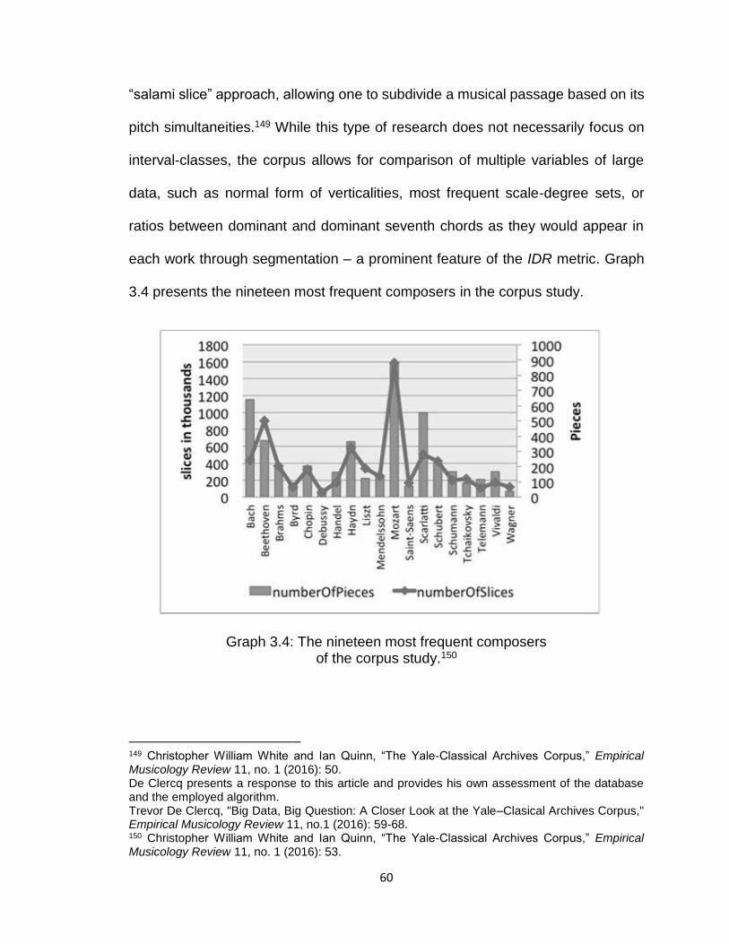
60

“salami slice” approach, allowing one to subdivide a musical passage based on its

pitch simultaneities.149 While this type of research does not necessarily focus on

interval-classes, the corpus allows for comparison of multiple variables of large

data, such as normal form of verticalities, most frequent scale-degree sets, or

ratios between dominant and dominant seventh chords as they would appear in

each work through segmentation – a prominent feature of the IDR metric. Graph

3.4 presents the nineteen most frequent composers in the corpus study.

Graph 3.4: The nineteen most frequent composers of the corpus study.150

149 Christopher William White and Ian Quinn, “The Yale-Classical Archives Corpus,” Empirical Musicology Review 11, no. 1 (2016): 50. De Clercq presents a response to this article and provides his own assessment of the database and the employed algorithm. Trevor De Clercq, "Big Data, Big Question: A Closer Look at the Yale–Clasical Archives Corpus," Empirical Musicology Review 11, no.1 (2016): 59-68. 150 Christopher William White and Ian Quinn, “The Yale-Classical Archives Corpus,” Empirical Musicology Review 11, no. 1 (2016): 53.

61

Graph 3.5 presents the most frequent scale-degree sets among all the

works in the corpus, as transposed to C major or C minor.151 This supports the

notion that the tonic triad is the predominant phenomenon in tonal works, occurring

9% of all times. Furthermore, this graph mathematically reveals that the works in

the corpus studies are principally based on the sub-elements of either tonic or

dominant. The nine most frequent sub-elements are the major tonic triad, ^5, ^1,

dominant seventh chord, minor tonic triad, dominant triad, as well as harmonic

intervals of C-E, C-G, and E-G, all of which constitute the tonic triad.

Graph 3.5: The most frequent scale-degree sets among all the works in the corpus, as transposed to C major or C minor.152

151 Ibid., 53-55. 152 Ibid., 55.

62

3.3. Calculating Harmonic Dissonance

As stated previously, the accurate representation of harmonic dissonance can be

achieved by combining the cognitivist and the physicalist methodologies.

Numerical analysis that generates data is what constitutes the mathematical side

of dissonance research. Dissonance that is measured can be ranked and

compared based on statistical analysis. Huron derives the term consonance index

to define a value that represents the perceived consonance between two

concurrent tones. The consonance index likewise presents a particular weight to

each interval-class. It is important to note that from a mathematical perspective,

the accurate representation of consonance index would disregard aspects, such

as sound pressure level and pitch register, even though these are essential

components of acoustical and psychological dissonance.153

Huron constructs an index of tonal consonance based on the experimental

data from previous studies by Malmberg (1918), Kameoka and Kuriyagawa (1969),

and Hutchinson and Knopoff (1978).154 All major, minor, and perfect intervals,

except for unisons and octaves were analyzed. The results can be seen in Tables

3.1, 3.2, and 3.3.

153 David Huron, “Interval-Class Content in Equally Tempered Pitch-Class Sets: Common Scales Exhibit Optimum Tonal Consonance,” Music Perception 11, no. 3 (Spring 1994): 292. 154 Ibid., 292. Akio Kameoka and Mamoru Kunyagawa, “Consonance Theory. Part I: Consonance of Dyads,” Journal of the Acoustical Society of America 45 (1969): 1451–1459. Akio Kameoka and Mamoru Kunyagawa, “Consonance Theory. Part II: Consonance of Complex Tones and its Calculation Method,” Journal of the Acoustical Society of America 45 (1969): 1460-1469. C. F. Malmberg, "The Perception of Consonance and Dissonance," Psychological Monographs 25, no. 2 (1918): 93-133. W. Hutchinson and L. Knopoff, “The Acoustic Component of Western Consonance,” Interface 7 no. 1 (1978): 1-29. W. Hutchinsonand L. Knopoff, “The Significance of the Acoustic Component of Consonance in Western Triads,” Journal of Musicological Research 3 (1979): 5-22.

63

Table 3.1: Index of tonal consonance, based on the experimental data from studies by Malmberg.155

Consonance

Interval Level of Consonance

minor second 0.00

major second 1.50

minor third 4.35

major third 6.85

perfect fourth 7.00

tritone 3.85

perfect fifth 9.50

minor sixth 6.15

major sixth 8.00

minor seventh 3.30

major seventh 1.50

Malmberg’s study is ranked on the increasing scale with the lowest value of

0.00 being highly dissonant. According to Malmberg’s work, the minor second is

the most dissonant interval while the perfect fifth and the perfect fourth are the

most consonant intervals. Hutchinson’s and Knopoff’s study is ranked on the

decreasing scale with the lowest value of 0.0221 being highly consonant. As

Malmberg, Hutchinson and Knopoff present the perfect fourth and the perfect fifth

155 David Huron, “Interval-Class Content in Equally Tempered Pitch-Class Sets: Common Scales Exhibit Optimum Tonal Consonance,” Music Perception 11, no. 3 (Spring 1994): 293.

64

as a consonant interval. Unlike Malmberg, Hutchinson and Knopoff present the

minor seventh as the most dissonant interval.

Table 3.2: Index of tonal dissonance, based on the experimental data from studies by Hutchinson and Knopoff.156

Dissonance

Interval Level of Dissonance

minor second 0.4886

major second 0.2690

minor third 0.1109

major third 0.0551

perfect fourth 0.0451

tritone 0.0930

perfect fifth 0.0221

minor sixth 0.0843

major sixth 0.0477

minor seventh 0.0998

major seventh 0.2312

Finally, Kameoka’s and Kuriyagawa’s study is based on the decreasing

scale with the lowest value of 215 being highly consonant. According to Kameoka’s

and Kuriyagawa’s research, the minor second is the most dissonant interval and

the perfect fifth is the most consonant interval.

156 Ibid., 293.

65

Table 3.3: Index of tonal dissonance, based on the experimental data from studies by Kameoka and Kuriyagawa.157

Dissonance

Interval Level of Dissonance

minor second 285

major second 275

minor third 255

major third 250

perfect fourth 245

tritone 265

perfect fifth 215

minor sixth 260

major sixth 230

minor seventh 250

major seventh 255

Although all three studies show that the minor sixth is more consonant than

the major third, such a difference is irrelevant, since both intervals are

complementary and belong to the same interval-class.158 Huron compiles the three

studies into one. In this instance, the complementary intervals are combined (such

as minor second and major seventh, major second and minor seventh, minor third

and major sixth, as well as perfect fourth and perfect fifth). Table 3.4 shows the

157 Ibid., 293. 158 Ibid., 293.

66

combined intervals that generate interval-classes, as well as an appropriate

consonance index for each interval-class.159

Table 3.4: Normalized data set of combined interval-class index.

Interval-Class Consonance

minor second / major seventh -1.428

major second / minor seventh -0.582

minor third / major sixth +0.594

major third / minor sixth +0.386

perfect fourth / perfect fifth +1.240

augmented fourth / diminished fifth -0.453

It is also important to mention LoPresto’s work on measuring musical

consonance because his research, similar to the IDR, bases the dissonance metric

on the frequency of different intervals under equal temperament tuning system.160

Such a mathematical approach of calculating dissonance measures intervals

according to the order of merit, ranking them from the most consonant to the most

dissonant.161 This method predominantly focuses on harmonic dyads and does not

combine them into larger harmonic structures, such as triads or seventh chords.

The order of merit, as per LoPresto, can be seen in Table 3.5.

159 Ibid., 293. 160 Michael C LoPresto, “Measuring Musical Consonance and Dissonance,” The Physics Teacher 53, no. 4 (2015): 226. 161 Ibid., 226.

67

Table 3.5: LoPresto’s order of merit table.

Interval P8 P5 M6 M3 P4 m6 m3 trit. m7 M2 M7 m2

Order of merit 1 2 3 4 5 6 7 8 9 10 11 12

The scholarship mentioned above deals with various types of consonant

and dissonant intervals. In addition, there has been research in the past that looks

at dissonant intervals and the many ways of providing harmonic resolutions. In his

works, Yavorksy deals with tritones – the most unstable harmonic interval in

music.162 Yavorsky designs a music system that looks at all possible resolution of

tritone towards consonance, or of the tritone towards dissonance, followed by

consonance.163 Yavorsky focuses on the tritone as the nucleus of a harmonic

progression.

Figure 3.1 provides two examples of “gravitational pulls,” which are possible

for a tritone that requires resolution towards imperfect consonance.164 In the first

example, the upper pitch of the tritone is resolved by a descending minor second,

while the lower pitch of the tritone is resolved by an ascending minor second. This

generates a resolution towards the interval of a major third. In the second example,

the upper note of the tritone is resolved by an ascending minor second, while the

lower pitch of the tritone is resolved by a descending minor second. This generates

a resolution towards the interval of a minor sixth – the inverse of a major third. In

162 William Drabkin, "Tritone," Groves Music Online (2008). http://www.oxfordmusiconline.com/subscriber/article/grove/music/28403. 163 Mark Aranovsky, “Теория и Концепция Яворского,” Искуство Музыки: Теория и История 6 (2012): 49. 164 Ibid., 50.

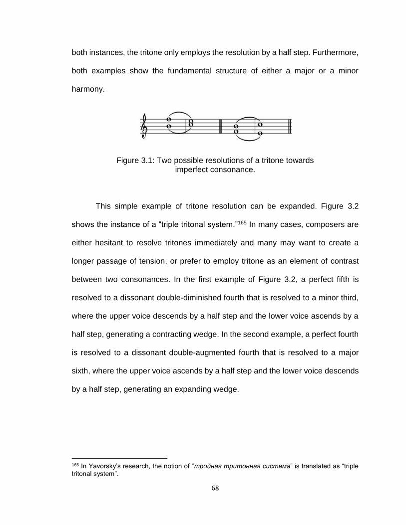
68

both instances, the tritone only employs the resolution by a half step. Furthermore,

both examples show the fundamental structure of either a major or a minor

harmony.

Figure 3.1: Two possible resolutions of a tritone towards imperfect consonance.

This simple example of tritone resolution can be expanded. Figure 3.2

shows the instance of a “triple tritonal system.”165 In many cases, composers are

either hesitant to resolve tritones immediately and many may want to create a

longer passage of tension, or prefer to employ tritone as an element of contrast

between two consonances. In the first example of Figure 3.2, a perfect fifth is

resolved to a dissonant double-diminished fourth that is resolved to a minor third,

where the upper voice descends by a half step and the lower voice ascends by a

half step, generating a contracting wedge. In the second example, a perfect fourth

is resolved to a dissonant double-augmented fourth that is resolved to a major

sixth, where the upper voice ascends by a half step and the lower voice descends

by a half step, generating an expanding wedge.

165 In Yavorsky’s research, the notion of “тройная тритонная система” is translated as “triple tritonal system”.

69

Figure 3.2: Two possible examples of “triple tritonal system.”

The theories of Yavorsky are based on the idea that harmonic intervals build

harmonies, rather than chords. Furthermore, Yavorsky generates multiple

common approaches how dissonance, such as tritone, can be used in the Western

music. Chopin establishes the importance of tritone in many of his works.166 The

tritone is an interval that exists in many chords used by Chopin to create

dissonance, which include augmented sixth chords and seventh chords.

3.4. Chopin’s Connection

Chapter 2 covered the basics of Schenkerian methodology to understand the

theory and the pianism of the four études. The various graphs of Schenkerian

analysis can trace the vertical tension both on local and global levels, as seen in

the foreground and the background readings of the four works. In music of Chopin,

dissonance generates musical diversity and allows for necessity to gravitate

towards consonance, since the dissonant inferences created by a composer in the

melodic and harmonic processes must be resolved and finalized.167 One of the

166 George Rochberg, A Dance of Polar Opposites: The Continuing Transformation of Our Musical Language (Rochester, NY: Rochester University Press, 2012), 58. 167 Reed J. Hoyt, “Harmonic Process, Melodic Process, and Interpretive Aspects of Chopin’s Prelude in G Minor,” Indiana Theory Review 5, no. 3 (Spring 1982): 22.

70

ways to construe tension in music is through the means of implication and

realization.

According to Meyer, the implicative relationships in music allow the listener

to link multiple musical phenomena.168 Therefore, an implication, such as harmonic

dissonance, is connected to a realization – its resolution. For composers such as

Chopin, it is a matter of when to realize an implication and for how long such

implicative relationship is to be held before proceeding onto the next one. Figure

3.3 presents example of implied dissonance, taken from Meyer’s Explaining Music:

Essays and Explorations. The example consists of a small passage of six

measures and its two Schenkerian representations.

In this example, the middle graph is of most significance. In Graph B, the

implied dissonance is indicated in the analysis by the tied note C, where “the falling

seventh (C♯ to D♯) creates an implied dissonance so that the following B acts as

the resolution of an imagined suspension.”169 Another example of dissonance is

morphological, where a passage serves as a finale of one melody and the

initialization of another.170 An instance of such phrasal intersection is where the

"resolution enhances the sense of satisfaction and closure."171

168 Leonard B. Meyer, Explaining Music: Essays and Explorations (Berkeley, CA: University of California Press, 1973), 116. 169 Ibid., 168. 170 Meyer labels such occurrence as “elision.” 171 Ibid., 233.

71

Figure 3.3: An example of implied dissonance, as taken from Meyer’s Explaining Music: Essays and Explorations.172

The I-R model is likewise related to the notion of musical closure, since a

strong implication weakens the closure and a strong closure weakens one’s

perception of the implication.173 Dissonance, as a musical component, can

determine and increase the strength of the implication, as well as have an influence

on the type and quality of the resolution, which depends on the compositional

strategy of a composer.174 Dissonance can likewise "displace the implied location

of a melodic realization."175 From perspective of music theory, dissonant elements

can function in multiple ways, beneficial to reaching the resolution. An example

can be seen in Chopin's Mazurka Op. 17, no. 1, mm. 9-11 (Figure 3.4). This

172 Ibid., 168. 173 Eugene Narmour, “Implication – Realization: Continuous Bottom-Up Non-Closure Versus Top-Down Closural Structuration,” in Music in the Social and Behavioral Sciences: An Encyclopedia, ed. William Forde Thompson (Paris: Saga Publications, 2014), par. 1. 174 Eugene Narmour, The Analysis and Cognition of Melodic Complexity: The Implication-Realization Model (Chicago: The University of Chicago Press, 1992), 61. 175 Ibid., 177.

72

passage begins with a large melodic leap from C to B♭. The next significant

component of dissonance, the F♯, occurs on the first beat of m. 10; this pitch breaks

off the descending pattern that was started in m. 9 (B♭-A-F♯) and initializes a

melodic motion in an opposite direction towards (F♯-G-A), which ends on the

second beat of m. 10 before reaching the closure with a stepwise descent to G on

the third beat of m. 10.

Figure 3.4: Chopin’s Mazurka Op. 17 No. 1, mm. 9-10.176

From the perspective of harmony, the clearest and the simplest approach

to realize a dissonant passage is to resolve such passage on a major or minor

consonance. This can be seen in mm. 67-70 Op. 10 No. 3, shown in Figure 3.5.

Chopin generates a string of dissonant implications that are realized through pure

consonances. Three of the many instances, where a model of implication-

realization can be applied, are in m. 67, m. 68, and mm. 69-70. In m. 67, the E7

harmony that spans through beats 1-4 is realized on A major harmony on beat 5,

generating a V7/IV – IV progression. Similar concept exists in m. 68, where the G♯7

harmony on beats 1-4 is realized through the C♯ major harmony on beat 5,

generating a V7/vi – vi progression. Finally, the dominant seventh and the French

176 Ibid., 199.

73

augmented harmonies in m. 69 are realized through the E major harmony in m.

70.


These examples of implication and realization are likewise significant from

perspective of performance practice. One of the artistic elements that a pianist

applies to signify the moments of dissonance and consonance is rubato. The

methodology of rubato changed throughout the history of performance. In Chopin’s

works, the notion of rubato depends on one’s “interpretation,” “individuality,” and

the amount of musical meaning that a pianist wishes to apply to an element, such

as consonance and dissonance.177 The flexibility of tempo that a pianist chooses

for a passage can be understood through musical connotations and stylistic

features of the work.178 The composer himself, for instance, preferred to play the

melody with more rhythmic freedom while keeping the accompaniment close to

instructed tempo.179 This is because Chopin was one of the first pianists to apply

the word rubato as a "direction in a performance" and not simply as “tempo

177 Thomas Fielden, "Tempo Rubato," Music & Letters 23, no. 1 (April 1953): 151. 178 Sandra P. Rosenblum, "The Uses of Rubato in Music, Eighteenth to Twentieth Centuries," Performance Practice Review 7, no. 1 (Spring 1994), 43. 179 Jean-Jacques Eigeldinger, Chopin: Pianist and Teacher as Seen by his Pupils (Cambridge: Cambridge University Press, 1986),250.

74

adjustment”.180 This occurred as a result of 19th-century performance practice

being more flexible and allowing for a more varied interpretational possibilities.181

Contrary to modern performance practice, Chopin's innovative comprehension of

tempo rubato represented a "slight delay of the melody with respect to the bass.182

The preceding discussion summarizes the important elements on which the

Interval Dissonance Rate will be based. The mathematical and acoustical research

presented in previous scholarship allowing one to define and apply the notion of

harmonic dissonance to the analysis of Chopin’s compositions. Furthermore,

previous approaches to dissonance generate scholarly knowledge, on which the

IDR tool is based on, and which leads to a better understanding of Chopin’s many

contributions to harmony and vertical tension.

180 Richard Taruskin, Music in the Nineteenth Century: The Oxford History of Western Music (Oxford: Oxford University Press, 2010). 181 Nicholas Cook, Beyond the Score: Music as Performance (Oxford: Oxford University Press, 2013), 174. 182 Richard Taruskin, Music in the Nineteenth Century: The Oxford History of Western Music (Oxford: Oxford University Press, 2010).

75

CHAPTER 4. THE INTERVAL DISSONANCE RATE TECHNIQUE

4.1 About Interval Dissonance Rate

The computational approach to intervallic breakdown of a musical passage (or

larger structures) provides beneficial results, as seen in works of Malmberg,

Hutchinson & Knopoff, Kameoka & Kuriyagawa, LoPresto, and Huron. In their

research, however, all intervals are ranked based on their respective level of

consonance and dissonance. Nevertheless, the dissection of every possible

harmonic interval presents an opportunity to focus on harmonies from perspective

of any two concurrently played notes.183 Furthermore, the segmentation analysis

allows for equal analytical comparison of any verticality that is found in the score.

The IDR will employ segmentation to analyze for harmonic dissonance, dissecting

all possible harmonic dyads in the opening four études of Op. 10. Such practice

combines the musical analysis with a mathematical approach and the proposed

methodology diminishes the level of subjectivity by emphasizing the objective

theoretical examination of musical tension in Chopin’s compositions.184

The IDR is an analytical system that measures the amount of harmonic

dissonance and is based on a formula that can be applied to any piece of tonal

music that contains vertical tension. The proposed system calculates the relative

percentage of dissonant vertical intervals (that will be labeled as the DI group) and

consonant vertical intervals (that will be labeled as the CI group). Furthermore, the

IDR integrates analytical and scientific evaluations in non-monophonic Western

music, using a modified interval-class vector (modicv) that incorporates the

183 The technique of IDR incorporates vertical dissection employing harmonic dyads. 184 It is important to note that musical tension in a composition is considered a subjective concept.

76

frequency of recurrent pitches (pn), where the collection of DI and CI intervals

contains two sets of four modified interval-classes (ic). The DI and CI groups

combine to generate a set of all possible harmonic intervals (TI).

The traditional interval-class vector (icv) is a string of six digits, where each

numeral represents one of the six interval-classes, based on the number of

semitones (s).185 The icv, with elements such as <x1, x2, x3, x4, x5, x6>, consists of

the following:

• The element <x1> denotes the total amount of minor seconds (1s), major

sevenths (11s), and equivalent intervals.

• The element <x2> denotes the total amount of major seconds (2s), minor

sevenths (10s), and equivalent intervals.

• The element <x3> denotes the total amount of minor thirds (3s), major sixths

(9s), and equivalent intervals.

• The element <x4> denotes the total amount of major thirds (4s), minor sixths

(8s), and equivalent intervals.

• The element <x5> denotes the total amount of perfect fourth (5s), perfect

fifths (7s), and equivalent intervals.

• The element <x6> denotes the total amount of tritones (6s) and equivalent

intervals.

185 Michiel Schuijer, Analyzing Atonal Music: Pitch-Class Set Theory and Its Contexts (Rochester, NY: University of Rochester Press, 2008), 47.

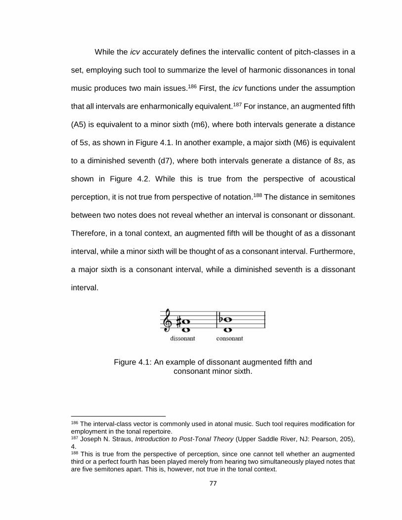
77

While the icv accurately defines the intervallic content of pitch-classes in a

set, employing such tool to summarize the level of harmonic dissonances in tonal

music produces two main issues.186 First, the icv functions under the assumption

that all intervals are enharmonically equivalent.187 For instance, an augmented fifth

(A5) is equivalent to a minor sixth (m6), where both intervals generate a distance

of 5s, as shown in Figure 4.1. In another example, a major sixth (M6) is equivalent

to a diminished seventh (d7), where both intervals generate a distance of 8s, as

shown in Figure 4.2. While this is true from the perspective of acoustical

perception, it is not true from perspective of notation.188 The distance in semitones

between two notes does not reveal whether an interval is consonant or dissonant.

Therefore, in a tonal context, an augmented fifth will be thought of as a dissonant

interval, while a minor sixth will be thought of as a consonant interval. Furthermore,

a major sixth is a consonant interval, while a diminished seventh is a dissonant

interval.

Figure 4.1: An example of dissonant augmented fifth and consonant minor sixth.

186 The interval-class vector is commonly used in atonal music. Such tool requires modification for employment in the tonal repertoire. 187 Joseph N. Straus, Introduction to Post-Tonal Theory (Upper Saddle River, NJ: Pearson, 205), 4. 188 This is true from the perspective of perception, since one cannot tell whether an augmented third or a perfect fourth has been played merely from hearing two simultaneously played notes that are five semitones apart. This is, however, not true in the tonal context.

78

Figure 4.2: An example of consonant major sixth and dissonant diminished seventh.

Figure 4.3 present a C augmented triad and an A♭ augmented triad in first

inversion. Both triads employ the root, the third, and the fifth as chordal factors.

Correspondingly, both triads contain identical pitch-classes and are represented

by the same normal form (048).189 However, in a tonal context, these triads are

notated in different ways and while a C augmented triad and an A♭ augmented

triad in first inversion share an identical icv, both serve diverse functions in a tonal

context. The initial triad in Figure 4.3 consists of two major thirds and an

augmented fifth, while the latter triad consists of a major third, a diminished fourth,

and a minor sixth. Therefore, enharmonic equivalence should not be utilized when

working with dissonance in the Romantic period music of Chopin.

Figure 4.3: The C+ and A♭+6 triads with different

intervallic makeups. 190

189 The notion of prime and normal forms does not change when applying the modified interval-class vector. 190 The symbol “+” represents an augmented triad and the symbol “–” represents a diminished triad.

79

Second, the traditional icv does not incorporate recurrent pitches and

therefore, does not present an interval-class that signifies unisons, octaves, and

equivalent harmonic intervals. Since the icv is predominantly used for post-tonal

music, the inclusion of such an interval-class is not necessary.191 Nevertheless,

unisons and octaves are prominent intervals in tonal music, particularly in the

works of Chopin.192 The significance of such interval-class in Chopin’s Études Op.

10 Nos. 1-4 will be shown in Chapter 5. The unisons, octaves, and similar intervals

generate major and minor triads, which are the fundamental musical elements for

construction of tonal works. The number of times that a pitch repeats in a harmonic

set is an important concept of calculating for dissonance, since the reinstated

pitches create additional harmonic verticalities that must be included into the

computational analysis.

Figure 4.4 shows two different sets of notes with identical icv. While the

intervallic content of both sets is alike, the cardinality is not.193 As shown, the only

source of dissonance in D-F-B is the single tritone between pitches F and B. On

the contrary, the second set has a cardinality of five, with pitches D and F repeated.

The second chord incorporates more tension with the supplementary notes,

producing two tritones.

191 David Huron, “Interval-Class Content in Equally Tempered Pitch-Class sets: Common Scales Ehxibit Optimum Tonal Consonance,” Music Perception: An Interdisciplinary Journal 11, no. 3 (Spring, 1994): 292. 192 Jim Samson, Chopin Studies, Volume 1 (Cambridge: Cambridge University Press, 1988), 145. An example can be seen in Chopin’s Étude Op. 10 No. 1, where the composer utilizes only the unisons and octaves throughout the whole work in the left hand. 193 For more information on function of a set based on its cardinality, see Eric J Isaacson, “Similarity of Interval-Class Content Between Pitch-Class Sets: The ICVSIM Relation,” Journal of Music Theory 34, no. 1 (Spring 1990).

80

Figure 4.4: Two identical B- chords with same icv, but with a different level of dissonance.

4.2. The modified icv

The modicv is derived from the Morris’s notion of a multiset.194 The modicv is a

revised version of icv, modified to accurately represent the intervallic content of

tonal music. The total number of intervals (TI) found in modicv consist of two

intervallic groups – the consonant intervals groups (CI) and the dissonant intervals

group (DI), where each group holds four modified interval-classes. Each interval

must belong to a group and no interval may belong to more than one icx. The

interval-classes of modicv are as follows:

• The element <c1> consists of consonant intervals, such as unisons (0s),

octaves (12s), and equivalent intervals.

• The element <c2> consists of consonant intervals, such as minor third (3s),

major sixth (9s), and equivalent intervals.

• The element <c3> consists of consonant intervals, such as major third (4s),

minor sixth (8s), and equivalent intervals.

194 Morris incorporates the use of multisets to include the multiple occurrences of pitch-classes in a set. Robert Morris, “Mathematics and the Twelve-Tone System: Past, Present, and Future,” Perspectives of New Music 45, no. 2 (Summer, 2007): 98.

81

• The element <c4> consists of consonant intervals, such as perfect fourth

(5s), perfect fifth (7s), and equivalent intervals.

• The element <d1> consists of dissonant intervals, such as minor seconds

(1s), major sevenths (11s), and equivalent intervals.

• The element <d2> consists of dissonant intervals, such as major seconds

(2s), minor sevenths (10s), and equivalent intervals.

• The element <d3> consists of dissonant intervals, such as tritones (6s), and

equivalent intervals.

• The element <d4> consists of all dissonant intervals that are enharmonically

equivalent to consonances.

It is important to mention that the ideas of consonance and dissonance are

context-specific and many intervals can be thought of as both consonant and

dissonant, depending on the music period and genre. The IDR focuses on defining

consonant and dissonant intervals, based on the pre-20th century view of Western

tonality. Therefore, while such system is appropriate for Chopin’s music and

presents definite results, it would require modification and adjustment, when

working with compositions of other composers, such as Debussy, or non-classical

styles, such as jazz music.195

195 For more information on dissonance in Debussy’s music, refer to: Robert Schmitz, The Piano Works of Claude Debussy (New York: Dover, 1966). For more information on dissonance in jazz music, refer to: Ajay Heble, Landing on the Wrong Note: Jazz, Dissonance, and Critical Practice (London: Routledge, 2000).

82

One of the notable examples is the understanding of musical tension in

major and minor thirds, since such intervals were considered as dissonant in the

pre-Odington era and as consonant in the post-Odington period.196 Another

example is the perception of the harmonic ninths. According to the IDR, a minor

and a major ninth is equivalent to a minor and a major second and therefore, both

are to be considered as dissonant intervals. Such instance can be seen in Figure

4.5 in mm. 1-7 of Scriabin’s Trois Études Op. 65 No. 1, where a series of ninths

generate a dissonant harmony in the need of resolution.197 Such resolution,

however, never occurs.

Figure 4.5: Scriabin’s Trois Études Op. 65 No. 1, mm. 1-7.

196 Jeffrey Pulver, "Walter Odington: The Consonance of the Third, and the Common Chord," The Musical Times 69, no. 1030 (December 1928): 1086. 197 This is an instance of Scriabin’s late period works, where the composer bases the whole composition on the interval of a ninth.

83

However, a ninth in the works of Debussy, whose compositional strategy

includes consideration for and emphasis on sevenths, ninths, and eleventh chords,

sounds consonant.198 This can be seen in Figure 4.6 in m 13-15 of La Cathédrale

Engloutie. In this instance, the ninth is generated from the lowest and the highest

pitches of the left hand in mm. 14-15. Such series of harmonies is tonally stable

and is not in need of resolution.

Figure 4.6: Debussy’s La Cathédrale Engloutie, mm. 13-15.

As mentioned in Chapter 2, one of the most common approaches to working

with harmonic dissonance involves the ranking of harmony from least to most

consonant. While the IDR does not rank the dissonances, it bifurcates them

between two groups.199 The CI-group contains a total of eight intervals.200 These

include four perfect intervals, two major intervals, and two minor intervals: perfect

unison, minor third, major third, perfect fourth, perfect fifth, minor sixth, major sixth,

198 Such a unique treatment of harmony is not a frequent occurrence in the common-practice period of the Western music, yet the use of sevenths, ninths, and elevenths is an important characteristic of Debussy’s compositional style. 199 The IDR can likewise calculate the frequency of a specific ic found in the score. For instance, Scriabin incorporates 16.5% of ic(d2) in Prelude Op. 11 No. 2 in A minor. This accounts for 56.16% of total dissonance found in the work. Nikita Mamedov and Robert Peck, “The Interval Dissonance Rate: An Analytical Look into Chromaticism of Chopin’s Op. 10 No. 2 and Scriabin’s Op. 11 No. 2” in Proceedings of Bridges 2017 (Phoenix, AZ: Tessellations Publishing, 2017), 478. 200 There are four sub-groups of the cx, where each cx contains two intervals.

84

and perfect octave. The DI-group amalgamates minor, major, diminished, and

augmented intervals: minor second, major second, tritone, minor seventh, major

seventh, as well as all possible diminished and augmented intervals.201 Figure 4.7

shows the range of possible TI subdivisions.

Figure 4.7: The generation of the eight ic for construction of IDR.

There are two steps that need to be taken to calculate the IDR of a harmonic

set. First, one needs to calculate the modicv. Second, one needs to divide the DI

group by the sum of all possible intervals (TI). The IDR is calculated based on the

following conditions:

IDR (%) = TI / DI, where {CI & DI} = modicv(x) + pn DI = {d1, d2, d3, d4}; CI = {c1, c2, c3, c4}

4.3. The IDR of Trichords, Tetrachords, and Pentachords

Functional harmony in a tonal composition tends to heavily rely on the four main

types of triads that appear in a diatonic scale, shown in Figure 4.8: major, minor,

diminished, and augmented. The major and the minor triads are consonant, while

201 Every possible interval in both CI and DI groups can have a diminished and an augmented interval. Therefore, for each major, minor, or perfect interval, there exist two possible ic(d4) intervals.

85

the diminished and the augmented triads are dissonant. Both major and minor

triads have two similar features: an identical prime form (047) and an identical icv

of <001110>. Furthermore, both major and minor triads in root position generate a

total of three intervals: a minor third, a major third, and a perfect fifth. However, the

order of the major and the minor thirds in each triad, which is influenced by the

location of the third scale degree, makes the major and the minor triads different.

The modicv of both triads is <01110000>. Since each triad consists of three

pitches, one can conclude that CI = 3 and DI = 0. Therefore, the IDR of C-E-G and

C-E♭-G is 0.00%, (as 0/3 = 0). It is also important to note that the number of pn will

not affect either of these triads, since no dissonant intervals exist.

Figure 4.8: The IDR of C major, C minor, C diminished, and C augmented triads.

The diminished triad in root position that is made of three notes contains

two stacked minor thirds and a diminished fifth. The prime form of a diminished

triad is (036) and its icv is <002001>. The diminished fifth is the source of

dissonance in this triad. The modicv of a diminished triad is <02000010>. Based

on the modicv, it is evident that CI = 2, DI = 1, and IDR = 33.33%. A root-position

augmented triad of identical cardinality contains two stacked major thirds and an

augmented fifth. Its prime form is (048) and its icv is <000300>. The modicv of an

augmented triad is <00200001>. Based on the modicv, it is evident that CI = 2, DI

= 1, and therefore, the IDR = 33.33%. Since the IDR does not rank the intervals

86

on the level of dissonance, it can be concluded that the IDR of both diminished

and augmented triads are identical.

An augmented triad is an example of a situation in which the d4 interval-

class is used. Enharmonically speaking, the augmented fifth is analogous to a

minor sixth, and both are equal to eight semitones. This proves that the icv of a set

cannot be used to accurately calculate the dissonance rate. Based on the icv of an

augmented triad, its IDR would be identical to the IDR of purely consonant major

and minor triads.

While tonal music is principally based on major, minor, diminished, and

augmented triads, other three-note combinations likewise exist.202 Table 4.1

shows some of the trichords and their respective IDR. All trichords are ranked from

most dissonant to most consonant. The following table also contains the notes of

a triad, its icv, its modicv, as well as a possible musical location of such harmonic

set. Based on the level of dissonance that they produce, all trichords can be

perceived differently. However, the mathematical approach limits the IDR of all

trichords with no recurrent pitches to four dissonance levels: 0.00%, 33.33%,

66.66&, and 100.00%.203 This occurs because any three notes can produce only

202 There are multiple views on what constitutes a triad. Ronald Pen states that a triad is a set of three notes that must contain successive intervals of a third. Therefore, a triad requires a root, a third, and a fifth. On the contrary, Howard Hanson and Carlton Gamer state that a triad is a combination of any three unique pitches and there should not be any intervallic limitations in between such pitches. For clarity, any set of three consecutively played notes will be labeled as a trichord. Ronald Pen, Introduction to Music (New York: McGraw-Hill, 1992): 81. Howard Hanson, Harmonic Materials of Modern Music: Resources of the Tempered Scale (New York: Appleton-Century-Crofts, 1960). Carlton Gamer, "Some Combinational Resources of Equal-Tempered Systems", Journal of Music Theory 11, no. 1 (1967): 37, 46, 50–52. 203 0.00% will be known as Pure Harmonic Consonance. This will be a significant term in the analysis of Chopin’s Études.

87

three intervals.204 The larger the cardinality of a harmonic set, the higher variety of

dissonance there will be.

Table 4.1: Other common trichords with their respective IDR.

Harmonic Trichord <icv> <modicv> IDR% Description

[C-C♯-D] <210000> <00001101> 100.00% Subset of a chromatic scale

[C-C♯-D♯] <111000> <00000102> 100.00% Subset of an octatonic scale

[C-E-F♯] <100011> <00100110> 66.66% Subset of a whole-tone scale

[C-D-E] <020100> <00100200> 66.66% Subset of a whole-tone and diatonic scales

[C-D-F♯] <010101> <00100110> 66.66% Subset of a dominant seventh chord

[C-D-F] <011010> <01010100> 33.33% Subset of a diatonic scale

[C-C♯-E] <101100> <01100001> 33.33% Subset of a hexatonic scale

[C-E-F] <100110> <00111000> 33.33% Subset of a diatonic scale

[C-D-G] <010020> <00020100> 33.33% Subset of a diatonic scale

[C-E♭-G♭] <002001> <02000010> 33.33% A diminished triad

[C-E-G♯] <000300> <00200001> 33.33% An augmented triad

[C-E-G] <001110> <01110000> 0.00% Major triad

[C-E♭-G] <001110> <01110000> 0.00% Minor triad

204 The amount of TI in a set can be calculated by combinatorial probability formula, such as

C(n, r)! = n! / (n – r)!r! The variable n represents the number of notes in a harmonic set. Furthermore, r = 2, where r represents the possible combinations of an interval consisting of no more than two notes. Therefore, a harmonic set made of three notes produces three harmonic intervals; a harmonic set made of four notes produces six harmonic intervals; a harmonic set made of five notes produces ten harmonic intervals; and so on. E. T. Jaynes and G. Larry Bretthorst (ed.), Probability Theory: The Logic of Science (Cambrdige: Cambridge University Press, 2003): 1-758.

88

The trichords [C-C♯-D] and [C-C♯-D♯] produce an IDR of 100.00%. This

means that such harmonic sets will incorporate zero consonance. Most of the

trichords, however, will produce an IDR of either 33.33% or 66.66%, since there

will be at least one or two dissonances in the set. There are only a handful of

trichords that will produce a perfect harmonic consonance; an example of such

trichords are all major and minor triads.205

In addition to trichords, there are multiple types of seventh chords that exist

in Western music, all of which have distinct functions.206 The history of music

theory reveals a rich tradition of various composers who utilize seventh chords in

unique ways. Further, while the exact reasoning for the use of seventh chords lies

in the compositional approach of each individual composer, it is a truism that one

of the common purposes for the use of seventh chords is the generation of

harmonic tension. Each of the seventh chords, made up of four notes with no

recurrent pitches, will produce six harmonic intervals. Therefore, there are six

possible IDR rates for pitch collections that consist of four unique notes: 0.00%,

16.66%, 33.33%, 50.00%, 66.66%, 83.33%.

It is important to note, however, that while the analysis of IDR presents a

set of categorial variables when analyzing trichords and seventh chords, this is

diversified with the inclusion of additional intervals. For instance, a musical

passage with twenty harmonic intervals contains 190 dissonance possibilities. The

205 The major and minor triads are not the only three-note harmonic sets that combine to form perfect harmonic consonance. However, a perfect harmonic consonance must be based on at least one of the scale degrees of the tonic triad. 206 Samuel Reenan and Richard Bass, "Types and Applications of P3,0 Seventh-Chord Transformations in Late Nineteenth-Century Music," Music Theory Online 22, no. 2 (June 2016). Eytan Agmon, "The Bridges that Never Were: Schenker on the Contrapuntal Origin of the Triad and Seventh Chord," Music Theory Online 3, no. 1 (January 1997).

89

first four Chopin’s études contain few thousand harmonic intervals. For

comparison, the opening étude consists of 3196 harmonic intervals – the lowest of

the four works. Based on the combinatorial probability formula, there are a total of

5,105,610 possible IDR values with such number of harmonic intervals.

Graph 4.1 presents the contrast between the harmonic dissonance

according to IDR and Huron’s Optimum Consonance Measure. All values have

been normalized on the scale of 0-1, where 0 is equivalent to maximum

dissonance and 1 is equivalent to maximum consonance.

Graph 4.1: IDR and Optimum Consonance Measure comparison for trichords on a scale of 0 to 1, where 0 = highest level of

dissonance and 1 = highest level of consonance.

The IDR of 0.00% is possible in a four-note collection. However, an IDR of

0.00% is impossible in a seventh chord, since at least one of the intervals of the

seventh chord, (the seventh), will always be dissonant and be part of either

interval-class d3 or d4. The most frequent types of seventh chords in tonal music

are dominant seventh chord, minor seventh chord, leading tone seventh chord,

90

half-diminished seventh chord, and major seventh chord.207 Table 4.2 presents the

most common seventh chords in tonal music, its interval-class vector, modified

interval-class vector, and each chord’s respective IDR.

Table 4.2: Most common seventh chords with their respective IDR.

Harmonic Tetrachord Example <icv> <modicv> IDR%

Major seventh chord [C-E-G-B] <101220> <01221000> 16.66%

Minor seventh chord [C-E♭-G-B♭] <012120> <02120100> 16.66%

Minor major seventh chord [C-E♭-G-B] <101310> <01211001> 16.66%

Augmented major seventh chord [C-E-G♯-B] <101310> <01211001> 16.66%

Dominant seventh chord [C-E-G-B♭] <012111> <02110110> 33.33%

Half-diminished seventh chord [C-E♭-G♭-B♭] <012111> <02110110> 33.33%

Fully-diminished seventh chord [C-E♭-G♭-B♭♭] <004002> <02000022> 66.66%

Augmented minor seventh chord [C-E-G♯-B♭] <020301> <00200112> 66.66%

Diminished major seventh chord [C-E♭-G♭-B] <102111> <02001021> 66.66%

Dominant seventh flat five chord [C-E-G♭-B♭] <020202> <00200121> 66.66%

Graph 4.2 shows the comparison between the harmonic dissonance of

tetrachords according to IDR and Huron’s Optimum Consonance Measure. All

values have been normalized on the scale of 0-1, where 0 is equivalent to

maximum dissonance and 1 is equivalent to maximum consonance.

207 Stefan Kostka and Dorothy Payne, Tonal Harmony with an Introduction to Twentieth-Century Music (New York: McGraw-Hill Education, 2008), 225.

91

Graph 4.2: IDR and Optimum Consonance Measure comparison for tetrachords on a scale of 0 to 1, where 0 = highest level of

dissonance and 1 = highest level of consonance.

As stated previously, the frequency of recurrent pitches likewise plays a role

in the dissonance content of a harmony. This occurs because a supplemental note

(or a set of notes) can create additional interval-class verticalities in the makeup of

the TI. For instance, a dominant G7 chord, where each pitch is only used once, will

generate an IDR of 33.33%. This happens because the harmonic relationship

between pitches G, B, D, and F contains two dissonant and four consonant

intervals. However, if a supplementary pitch G is implemented to the dominant G7

chord, the IDR decreases to 30.00%. This occurs because the harmonic

relationship between pitches G, G, B, D, and F contains three dissonant and seven

consonant intervals. As evident, a difference of 3.33% exists while no new pitch-

classes are incorporated. This is shown in Figure 4.9.

92

Figure 4.9: The G7 chord with IDR of 33.33% and 30.00%.

The IDR of the two chords in Figure 4.10 has a difference of 3.33% – a small

change for a supplemental root note to generate. On the other hand, a similar

differential rate between two full pieces of music is significant enough to reveal a

stylistic change in the way both works generate harmonic dissonance. Typically,

consonance and dissonance in a piece of music can be produced by pitch doubling

and, therefore, the same notes can be employed to increase or decrease tension

in music. As seen from previous example, the IDR of a dominant seventh chord

that uses each of the pitches once is 33.33%.

Figure 4.10: The C7 chord with IDR of 13.33% and 40.00%.

On the contrary, the first chord in Figure 4.10 is a dominant seventh chord

that uses the fifth as a chordal factor three times, and the root, the third, and the

seventh scale degrees once, generating the IDR of 13.33%, creating a difference

of 20.00% when compared to a basic dominant seventh chord. The first chord in

93

Figure 4.10 contains thirteen dissonant and two consonant intervals. The second

chord in Figure 4.10 is a dominant seventh chord that uses the seventh scale

degree three times, and the root, the third, and the fifth scale degrees once,

generating the IDR of 40.00%, creating a difference of 6.66% when compared to

a basic dominant seventh chord and creating a difference of 26.66% when

compared to the first chord. In the second scenario, there are nine consonant

intervals and six dissonant intervals.

While not as frequent as the seventh chords, the ninth chords are likewise

significant to the harmony of Chopin’s music. In tonal music, the common practice

is to incorporate the 3rd, 7th, and the 9th scale degrees of the ninth chord, while

omitting the 5th scale degree.208 In this instance, the ninth chord is to be analyzed

as a tetrachord. However, there are occurrences, in which all five pitches of the

ninth chord are employed in a harmonic verticality. Table 4.3 shows a series of

ninth chords prominent to the analysis of Romantic music.

Table 4.3: The IDR analysis of ninth chords.

Harmonic Pentachords Example <icv> <modicv> IDR%

Minor ninth chord [C-E♭-G B♭-D] <122230> <02231200> 30.00%

Major ninth chord [C-E-G-B-D] <122230> <02231200> 30.00%

Dominant ninth chord [C-E-G- B♭-D] <032221> <02220310> 40.00%

Dominant minor ninth chord [C-E-G- B♭-D♭] <114112> <03111121> 50.00%

208 Bruce Benward and Marilyn Saker, Music in Theory and Practice, Volume 2 (New York: McGraw-Hill Companies, 2009), 183-184.

94

The dissonance range between the least dissonant chords (minor ninth and

major ninth) and the most dissonant chord (dominant minor ninth) is 20%.

However, two of the four chords share identical IDR. This occurs because the IDR

does not rank the intervals based on their dissonance level and therefore, if a

harmonic set has 10 interval-classes and three of them are dissonant, the IDR will

always be 30%.

4.4. Meter and Rhythm

Meter plays a significant role in the perception of consonance and dissonance. The

meter of a given work provides one with information regarding the strong and the

weak beats in each measure, as well as presenting a suggested sequence of

pulses. Furthermore, such emphasis on the strong and the weak beats changes

depending on the nature of the rhythm and alters our awareness of music tension.

Table 4.4 presents multiple examples of meter in music and provides an

appropriate time signature for each.

Table 4.4: Types and examples of standard meter.

Simple Duple Meter

2/2; 2/4; 2/8

Simple Triple Meter

3/2; 3/4; 3/8

Simple Quadruple Meter

4/2; 4/4; 4/8

Compound Duple Meter

6/4; 6/8; 6/16

Triple Compound Meter

9/4; 9/8; 9/16

Quadruple Compound Meter

12/4; 12/8; 12/16

The main beats in each meter are emphasized by the metric accents. For

instance, the first beat (the strong beat) of the 3/4 meter is accented, while the

95

second and the third beats (the weak beats) of 3/4 meter are unaccented. Other

types of accents, such as dynamic accent, tonic accent, and agogic accent are

likewise prominent. Whether part of melody or harmony falls on accentuated

division of the measure is an important conception both from theoretical and

performance perspectives, since accented beats will generate a higher level of

perceived dissonance. This occurs because of variance in the notions of internal

and external lengths of notes.209 The internal length of a note is how such note is

rhythmically represented in the score. From internal perspective, a metrically

accented quarter note is identical to metrically unaccented quarter note. However,

from external perspective, both notes would differ in duration, the concept that is

associated with performance practice. According to Caplin, this means that the

"position of the note within the measure is sufficient to impart accentuation in the

absence of any real durational or dynamic differentiation."210

Another important component of consonance and dissonance can be traced

through non-chord tones, some of which are suspensions, passing tones, and

neighbor tones. The placement of these non-chord tones likewise affects one’s

perception of consonance and dissonance. Figure 4.11 presents instances of two

harmonic successions. From the perspective of interval-class vector, both

examples can be represented identically: <001000>, <100000>, <001000>,

<010000>, and <000100>.

209 William E. Caplin, "Theories of Musical Rhythm in the Eighteenth and Nineteenth Centuries," in The Cambridge History of Western Music Theory, ed. Thomas Christensen (Cambridge: Cambridge University Press, 2008), 662. 210 Ibid., 662.

96

However, an evident difference exists in the way both passages sounds and

therefore, both structures will produce different perceptions of dissonance. The

second passage is generated by moving the top voice down the octave.

Furthermore, the lower voice is responsible for generating dissonance in the first

passage and the upper voice is responsible for generating dissonance in the

second passage.

Figure 4.11: Two passages with identical harmonic icv, but different perceptions of dissonance.211

Rhythm is one of the main characteristics of music that allows one to

understand a compositional language. The notion of rhythm amalgamates the

elements of pitch and duration, and therefore, influences the outcome of melodic

and harmonic dissonance.212 One of the ways how a composer may vary and

deviate the rhythm of a work is by using tuplets, allowing for division of a beat in

different number of subdivisions. In Chopin’s works, tuplets are essential to create

harmonic dissonance. The IDR treats tuplets the same way as other harmonic

rhythms. Figure 4.12 shows how a triplet will be dissected in the IDR analysis. In

this instance, the triplet is in the treble stave, while the regular rhythm is provided

211 Fred Lerdahl and Ray S. Jackendoff, A Generative Theory of Tonal Music (Cambridge: The MIT Press, 1983), 89. 212 Jeremy Pickens, Harmonic Modeling for Polyphonic Music Retrieval, PhD. Diss., University of Massachusetts, 2004: 12.

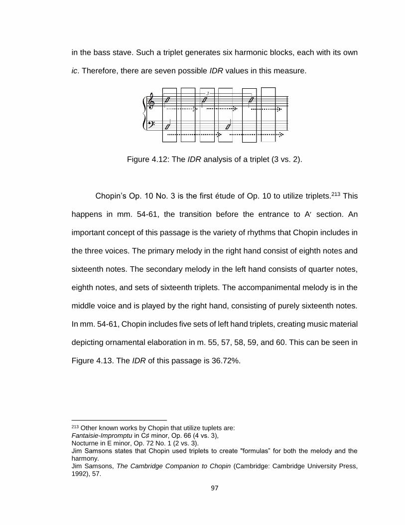
97

in the bass stave. Such a triplet generates six harmonic blocks, each with its own

ic. Therefore, there are seven possible IDR values in this measure.

Figure 4.12: The IDR analysis of a triplet (3 vs. 2).

Chopin’s Op. 10 No. 3 is the first étude of Op. 10 to utilize triplets.213 This

happens in mm. 54-61, the transition before the entrance to A section. An

important concept of this passage is the variety of rhythms that Chopin includes in

the three voices. The primary melody in the right hand consist of eighth notes and

sixteenth notes. The secondary melody in the left hand consists of quarter notes,

eighth notes, and sets of sixteenth triplets. The accompanimental melody is in the

middle voice and is played by the right hand, consisting of purely sixteenth notes.

In mm. 54-61, Chopin includes five sets of left hand triplets, creating music material

depicting ornamental elaboration in m. 55, 57, 58, 59, and 60. This can be seen in

Figure 4.13. The IDR of this passage is 36.72%.

213 Other known works by Chopin that utilize tuplets are: Fantaisie-Impromptu in C♯ minor, Op. 66 (4 vs. 3), Nocturne in E minor, Op. 72 No. 1 (2 vs. 3). Jim Samsons states that Chopin used triplets to create "formulas” for both the melody and the harmony. Jim Samsons, The Cambridge Companion to Chopin (Cambridge: Cambridge University Press, 1992), 57.

98


While Op. 10 Nos. 1-4 only contain one instance of tuplets, similar concept

can be applied to all tuplet subdivisions. Figure 4.14 presents how IDR analysis

dissects an instance of quadruplet.

Figure 4.14: The IDR analysis of a quadruplet (4 vs. 3).

4.5. The IDR of Opening Phrases in Op. 10 Nos. 1-4.

As mentioned earlier, the IDR can be used to test for dissonance of a specific

passage in music. The texture of each of Chopin’s études is dependent on the

technical challenge that the composer chose for each work. The following

99

subchapter presents the IDR analysis of the four opening phrases of Études Nos.

1-4, each with its own unique harmonic dissonance rate.

The opening phrase of Op. 10 No. 1 occurs in mm. 1-8. The phrase ends

with a half cadence that would go on to resolve to tonic in mm. 9-10. The IDR of

this phrase is 15.96%. The passage begins with purely consonant harmonies in

mm. 1,2, and 3, using only the root, the third, and the fifth chordal factors of C

major (tonic) and F major (subdominant) harmonies, before the harmonic

dissonance begins to increase. It is also important to note that the octaves in the

left hand generate the ic1 consonance at all times throughout the étude.

The opening phrase of Op. 10 No. 2 occurs in mm. 1-4. Much like the

opening phrase of Op. 10 No. 1, this phrase ends on a half cadence (E7). The IDR

of mm. 1-4 of the second étude is 16.51%. The harmonic consonance is created

from the major and minor triadic structures, found in the left hand’s accompaniment

and in the right hand’s inner voices. The harmonic dissonance, on the other hand,

is produced from the chromatic ascent and descent of the main melody of the

passage. For instance, the opening harmonic block in m. 1 contains the A minor

triad with IDR of 0.00%.214 However, the following harmonic block of m. 1 contains

the chromatic ascent of an augmented unison from A to A♯, generating dissonant

interval-classes between the pitch A♯ and the eighth note A, found in the left hand.

Another instance of an increase in dissonance occurs on the ninth harmonic block

of m. 2, where the pitch C♯, being a part of the chromatic path in the main melody,

214 Each measure in Op. 10 No. 2 contains a total of sixteen harmonic blocks.

100

contradicts the A minor harmony in the measure, generated in the left hand,

creating a harmonic tension between pitches C and C♯.

The opening phrase of Op. 10 No. 3 occurs in mm. 1-5. Similar to the

opening phrase of Op. 10 No. 1, this phrase is made up of three essential musical

layers: the main melody in the right hand, the secondary melody in the left hand,

and the inner voices in both right and left hands. Unlike the opening phrases of

Op. 10 Nos. 1 and 2, the opening phrase of the third étude consists of five

measures and ends on tonic of E major (perfect authentic cadence). The unique

characteristic of this phrase is the necessity of it to be performed unlike an étude,

incorporating a cantabile style and creating polyphonic depiction among the three

voices. The IDR of mm. 1-5 is 15.00%. This is a typical tonal Chopinesque melody

that reveals small traces of harmonic dissonance on unstable harmonies that need

resolution. This can be seen on the second beat of m. 1, where Chopin includes a

V7 harmony; the pitch A (seventh scale degree) is dissonant against the pitch B

(root) and the pitch D♯ (third). In this instance, the V7 harmony engulfs the full

second beat of m. 1, consisting of harmonic blocks 5-8, and the first beat of m. 2,

consisting of harmonic blocks 1-4. In both instances, the inner voice of the passage

interchanges pitch A, which is part of a pure consonance, and pitch B that

generates harmonic dissonance.

The opening phrase of Op. 10 No. 4 occurs in mm. 1-4. Like the opening

phrase in Op. 10 No. 3, Chopin chooses to employ an anacrusis measure to create

a stronger entrance into the tonic harmony. The harmonic dissonance is

implemented in mm. 1-5 of Op. 10 No. 3 in the inner voice. On the contrary, the

101

harmonic dissonance is implemented in mm. 1-4 of Op. 10 No. 4 in the main

melody in the right hand that consists of a series of sixteenth notes, which move

against the subordinate musical material in the left hand. When looking at the IDR

of the musical material found in the left hand, it is evident that the only harmonic

dissonance exists on beat four of m. 2 and beat two of m. 3. Nevertheless, the

inclusion of the right hand’s carrying the main melody of the étude generates

chromatic harmony and increases the level of harmonic tension with the IDR of

17.93%.

4.6. Computing Components of IDR

There are four components of the proposed technique: (1) pitch representation; (2)

interval-class representation; (3) range parameters; (4) the IDR calculations. The

pitch representation component allows one to turn the pitch name from the music

score into a number. The total of twelve recognized pitch-classes will generate

twelve values from 0 to 12. However, since the concept of enharmonic equivalence

does not exist in the IDR, this means that the same number cannot represent two

enharmonically equivalent pitches. Therefore, each note (n) will contain five

assigned values: double flat (♭♭), flat (♭), natural (♮), sharp (♯), and double sharp

(x).215 Since there exist seven unique notes in a diatonic scale, this generates a

total of thirty-five values for n. A variable (r) is used to represent a music rest and

does not carry any mathematical weight towards the analysis. The script can be

viewed in Appendix 9.

215 The script uses the “#” symbol to represent the “♯” and the “b” symbol to represent the “♭.” The

pitch is assumed as natural, if neither of the symbols are used.

102

Each harmonic interval is generated with the addition of two n values (the

combination of two pitch-classes). The sequence of all possible n values, such as

{0,1,3,7…} has an additive property, according to which the combination of any

two n values will never generate an identical answer, something that helps avoid

the enharmonic equivalence.

na + nb = na+b nc + nd = nc+d na+b – nc+d ≠ 0

There are 630 unique values that exist when any two n values are added.

This means that there are that many different harmonic intervals that exist between

any two notes of a diatonic scale, assuming octave equivalence. Each of the 630

values, which represent harmonic intervals, is assigned to one of the eight interval

classes of the modicv. This is done using a v-lookup table that allows one to match

icx to one of the 630 values. Each value can only belong to one interval-class.

The range parameters in the IDR analysis exist in order for one to select the

music that needs to be analyzed. The range parameter depends on the amount of

voices in the piece (or the passage). For instance, a composition with a maximum

of three musical layers, such as a, b, and c, will consist of three lines, each

representing an interval class ab, bc, and ac. This is the case with Chopin’s Étude

Op. 10 No. 1. On the contrary, Étude Op. 10 No. 2 contains a maximum of seven

musical layers, such as a, b, c, d, e, f, and g, generating twenty-one lines. The

parameters must state the beginning and the end of the chosen passage.

103

The IDR calculations are based on the parameters that are chosen for an

analysis. The IDR calculations consist of interval-class calculations, interval-group

calculations, and the final Interval Dissonance Rate calculations. The occurrence

of interval-class such as cx or dx is computed with the use of countif and indirect

functions. An indirect function is used because the range parameters are

references rather than statements that are written in. The CI and DI calculations

are computed by adding the cx and dx. Finally, the IDR is computed with diving the

total number of dissonant intervals by the total number of consonant intervals.

104

CHAPTER 5. QUANTIFYING CHOPIN’S ÉTUDES NOS. 1-4

5.1 Overview

The IDR calculations provide one with a large amount of quantitative data, which

allows for a broad assessable study of the four Chopin’s works. In addition, the

retrieved data allows one to focus on specific interval-classes and their relations

to Chopin’s music, his style of composition, and chromatic harmony. The IDR

results consist of statistical information that clarifies multiple components of

harmonic dissonance in the opening four études. These are:

1) Chopin’s most frequent dissonant interval-class is d2, which includes major

seconds, minor sevenths, and equivalent intervals.

2) The IDR analysis supports the notion that the use of chromaticism does not

result in a greater level of harmonic dissonance.

3) Each of the four B-sections are more dissonant than the average IDR of

their respective études. Likewise, the middle section is the most dissonant

part of each étude.216

Table 5.1 presents the results retrieved from the IDR analysis of Chopin’s

Op. 10 Nos. 1-4. For every étude, as well as each composition’s three sections of

the A-B-A form, the table shows the percentile values of the total interval

dissonance rate, as well as each distinct interval-class. The total percent of the

IDR is equivalent to the sum of the all four dissonant interval-classes. Based on

such an analysis, each interval-class in both consonant and dissonant groups is

216 The Average IDR of each étude consists of sections A, B, and A.

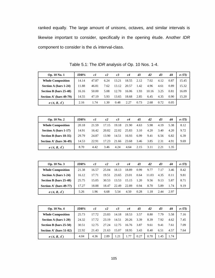
105

ranked equally. The large amount of unisons, octaves, and similar intervals is

likewise important to consider, specifically in the opening étude. Another IDR

component to consider is the d4 interval-class.

Table 5.1: The IDR analysis of Op. 10 Nos. 1-4.

Op. 10 No. 1 IDR% c1 c2 c3 c4 d1 d2 d3 d4 σ (TI)

Whole Composition 14.14 47.87 6.24 13.21 18.55 2.12 7.02 4.12 0.87 15.45

Section A (bars 1-24) 11.88 46.81 7.62 13.12 20.57 1.42 4.96 4.61 0.89 15.32

Section B (bars 25-48) 16.16 50.00 5.08 12.70 16.06 1.93 10.16 3.25 0.81 16.09

Section A (bars 49-79) 14.55 47.19 5.93 13.65 18.68 2.85 6.45 4.35 0.90 15.20

σ (A, B, A) 2.16 1.74 1.30 0.48 2.27 0.73 2.68 0.72 0.05



Section A (bars 1-17) 14.91 16.42 20.82 22.02 25.83 3.10 4.20 3.40 4.20 9.72

Section B (bars 18-35) 29.79 24.87 13.90 14.51 16.93 6.99 9.41 6.56 6.82 6.39

Section A (bars 36-49) 14.53 22.91 17.23 21.66 23.68 3.46 3.85 2.31 4.91 9.69

σ (A, B, A) 8.70 4.42 3.46 4.24 4.64 2.15 3.11 2.21 1.35



Section A (bars 1-24) 16.12 17.71 19.51 23.65 23.01 0.64 11.03 4.35 0.11 9.81

Section B (bars 25-48) 25.75 15.05 30.53 13.53 15.15 1.20 9.56 9.13 5.87 8.71

Section A (bars 49-77) 17.27 18.88 18.47 22.49 22.89 0.94 8.70 5.89 1.74 9.19

σ (A, B, A) 5.26 1.96 6.68 5.54 4.50 0.28 1.18 2.44 2.97



Section A (bars 1-20) 24.32 17.72 23.19 14.51 20.26 3.39 8.39 7.92 4.62 7.45

Section B (bars 25-50) 30.51 12.75 27.24 12.75 16.76 3.87 9.61 9.41 7.61 7.09

Section A (bars 51-82) 22.92 21.43 21.63 15.07 18.95 3.43 8.40 6.51 4.57 7.64

σ (A, B, A) 4.04 4.36 2.89 1.21 1.77 0.27 0.70 1.45 1.74

106

Due to the predominance of major and minor triads in the first étude, the d4

interval-class occurs less than 1% of the time. However, d4 is a significant interval-

class in the remaining three works and is especially emphasized in chromatic

passages. In addition, the table provides the standard deviation of all interval-class

rates and the standard deviation of each separate interval-class, based on its

occurrence in A, B, and A sections. Throughout the opening four études, Chopin

uses a varied set of harmonic interval-classes, as seen in diverse range of σ(TI).

On the contrary, unique interval-class rates in each of the three sections of every

étude tend to contain a lower range of σ(TI).

The average level of dissonance rises from the first to the fourth études.

Such an increase in IDR can be explained by the larger variety of harmonies,

something that can also be seen in the Schenkerian analysis. While there is no

definite dissonance for each pianistic technique that Chopin presents in the études,

it is evident that pure arpeggiation provides the least amount of harmonic

dissonance. The arpeggios are based on the root, third, fifth, and octave chordal

factors of each harmony. From a harmonic perspective, such a set will provide only

consonant intervals. From a melodic perspective, the level of dissonance will

depend on the supplementary musical material found in each harmonic slice.

Figure 5.1 shows the generation of all possible interval-classes in a root-position

major triad.

107

Figure 5.1: Modified interval-class vector generation of C major triad.

Figure 5.2 shows m. 51 of Op. 10 No. 1, as taken from the score – the

example of pure harmonic consonance. Table 5.2 provides the intervallic

breakdown of m. 51 that is generated form harmonic consolidation of notes F and

F, F and A, as well as F and C. Based on all possible harmonies of this passage,

only c1, c3, and c4 interval-classes exist and no types of ic(dx). The pianist is

expected to hold the octave in the left hand throughout the whole measure, which

explains the 47.83% frequency of the c1 interval-classes. Furthermore, m. 51

consists of sixteen beats, with the octaves and equivalent intervals generated on

beats 5, 9, and 13. In this example, ic(c2) that generates the interval of a minor

third or a major sixth does not exist.

Figure 5.2: Chopin’s Étude Op. 10 No. 1, m. 51.217

217 Frédéric Chopin, Études Op. 10 (Leipzig: C. F. Peters, 1879), 4.

108

Table 5.2: The intervallic breakdown of Chopin’s Étude Op. 10 No. 1, m. 51.

ic(c1) of m. 51 22/46 (47.83%)

ic(c2) of m. 51 0/46 (0.00%)

ic(c3) of m. 51 8/46 (17.39%)

ic(c4) of m. 51 16/46 (34.78%)

ic(d1) of m. 51 0/46 (0.00%)

ic(d2) of m. 51 0/46 (0.00%)

ic(d3) of m. 51 0/46 (0.00%)

ic(d4) of m. 51 0/46 (0.00%)

CI to DI ratio 46:0

IDR% 0.00%

The level of dissonance will increase with the reduction of arpeggiation. This

occurs because the arpeggios present outlines of major and minor triadic harmony,

which lowers the average IDR rate. When the number of interval-classes that

represent triadic harmony decreases, the ratio of dissonant to total intervals

increases, resulting in a higher IDR. Figure 5.3 shows the excerpt of m. 25 from

Op. 10 No. 4 and Table 5.3 presents the intervallic breakdown of the passage.

The IDR of m. 25 is 37.25%. The main reason for such a high level of

harmonic dissonance is the inclusion of double neighbor tones. The IDR

subdivides the measure into sixteen beats. Harmonic dissonance exists on beats

1-2, 5-6, 9-10, and 13-16. These beats contain multiple layers of music, as the

main melody in the right hand is supported by the chordal structure in the left hand

109

and in the inner voice of the right hand. Beats 3-4, 7-8, and 11-12 contain

monophonic melody in the right hand, as the left hand and the inner voices do not

carry any notes.

Figure 5.3: Chopin’s Étude Op. 10 No. 4, m. 25.218

Table 5.3: The intervallic breakdown of Chopin’s

Étude Op. 10 No. 4, m. 25.

ic(c1) of m. 25 12/51 (23.53%)

ic(c2) of m. 25 9/51 (17.65%)

ic(c3) of m. 25 5/51 (9.80%)

ic(c4) of m. 25 6/51 (11.76%)

ic(d1) of m. 25 3/51 (5.88%)

ic(d2) of m. 25 4/51 (7.84%)

ic(d3) of m. 25 5/51 (9.80%)

ic(d4) of m. 25 7/51 (13.72%)

CI to DI ratio 32:19

IDR% 37.25%

While the opening four études have an increasing rate of harmonic

dissonance, as based on the calculations of IDR, this is not the case for the rest of

218 Ibid., 12.

110

the opus, as the trend is broken at Op. 10 No. 5 – an étude in the key of G♭ Major,

where Chopin employs the arpeggiation, albeit in a different way than in Op. 10

No. 1.219 Nevertheless, the increasing dissonance rate is an important component

to consider from the perspective of performance practice, especially when

performing all études in one concert.220 There are multiple pianistic approaches

that a performer may choose to undertake, influenced by harmonic dissonance.

This can be seen in musical deviations in dynamics, tempo, texture, or the use of

pedals.

Graphs 5.1, 5.2, 5.3, and 5.4 present the frequency of all consonances and

dissonances in the four études in order, as they appear according to the modified

interval-class vector. The predominant interval-class in Op. 10 No. 1 is c1, which

occurs 47.87% of the time. The second most frequent interval-class is c4, which is

seen only 18.55% of the time. In the third and the fourth études, the interval-

classes are more dispersed. The most common interval-class in Op. 10 Nos. 3 and

4 is c2 and the least common interval-class is d1. Likewise, the d4 interval-class

varies, based on the technical skill that Chopin presents in each work. More varied

harmonies, as seen in Études Nos. 2 and 4 will generate a larger amount of d4

interval-classes. On the contrary, triadic configuration, as seen in Op. 10 No. 1

present the d4 interval-class less than 1% of the time.

219 Also nicknamed as the Black Keys étude, the arpeggiation model of Op. 10 No. 5 is based on the triplet configuration in the right hand, supported by the chordal accompaniment in the left hand. Another important characteristic of this work is that the melody in the right hand is played solely on black keys. 220 While an arduous task to accomplish, it is not an infrequent occurrence to find all works on the same program.

111

When it comes to harmonic dissonance in all four études, Chopin prefers to

use the d2 interval-class, which contains major seconds, minor sevenths, and

equivalent intervals. This interval-class is used between 3.85% to 11.03% of the

time throughout the analyzed works. The d2 interval-class occurs 3.85% of the time

in the A-section of Op. 10 No. 1 and 11.03% of the time in the A-section of Op. 10

No. 3. This is a significant interval, since it can be used to generate multiple types

of seventh chords, including dominant seventh chords, minor seventh chords, and

half-diminished seventh chords.221

Graph 5.1: All consonant and dissonant interval-classes in Op. 10 No. 1.

221 Refer to Table 4.2 of Chapter 4 regarding the modicv of various seventh chords and the location of ic(d2) in these chords.

0

5

10

15

20

25

30

35

40

45

50

as %

of

all n

ote

s

112



0

5

10

15

20

25

30

35

40

45

50

as %

of

all n

ote

s

0

5

10

15

20

25

30

35

40

45

50

as %

of

all n

ote

s

113


In all of these seventh chords, at least one interval-class of d2 exists when

such chord is in root position or in inversion. An example of this phenomena can

be seen in Figure 5.4 on the fourth beat of m. 54 of Étude Op. 10 No. 4. There are

thirteen d2 interval-classes out of possible sixty-six combinations. Table 5.4 reveals

the intervallic breakdown of the fourth beat of m. 54 with the IDR of 21.21%. It is

evident that on the final beat of the measure, ic(d2) is the most frequent dissonant

interval. The only other source of harmonic dissonance is a sole ic(d1). Therefore,

ic(d2) makes up a total of 92.86% of total dissonance in this excerpt. Moreover,

ic(d2) is the third most frequent interval on the fourth beat of m. 54 after ic(c4) and

ic(c2).

0

5

10

15

20

25

30

35

40

45

50

as %

of

all n

ote

s

114


Table 5.4: The intervallic breakdown of Chopin’s Étude Op. 10 No. 4, m. 54, beat 4.

ic(c1) of m. 54, beat 4 11/66 (16.66%)

ic(c2) of m. 54, beat 4 16/66 (24.24%)

ic(c3) of m. 54, beat 4 7/66 (10.60%)

ic(c4) of m. 54, beat 4 18/66 (27.27%)

ic(d1) of m. 54, beat 4 1/66 (1.52%)

ic(d2) of m. 54, beat 4 13/66 (19.70%)

ic(d3) of m. 54, beat 4 0/66 (0.00%)

ic(d4) of m. 54, beat 4 0/66 (0.00%)


IDR% 21.21%

In Romantic music, composers use chromaticism to produce tension and

generate musical variety, as well as to move between or replace two or more

diatonic harmonies.222 However, a larger use of chromaticism does not result in a

222 Dmitri Tymoczko, A Geometry of Music: Harmony and Counterpoint in the Extended Common Practice (Oxford: Oxford University Press, 2011), 21.

115

greater level of dissonance.223 The comparison can be made between the second

chromatic étude that is the second most harmonically consonant étude of the four

and the fourth piano étude that is the most harmonically dissonant of the four. In

this instance, the fourth étude is approximately on average 5.55% more dissonant

than the second étude. The most dissonant element of the second étude is the B-

section, which contains 29.79% of harmonic dissonance, while the most dissonant

section (of the twelve) in the first four compositions of Op. 10 is the B-section of

the fourth étude with the IDR of 30.51%.

Based on the IDR results, the B-section of each étude is more dissonant

than the average IDR of each respective étude. Likewise, the four middle sections

are the most dissonant parts of the first four études. This occurs because the A-

section seeks to present and establish the main thematic material of each

composition. Given the expository functions of the A-sections, this is not surprising.

The goal of middle sections is to develop the material presented in the opening

sections, directly or non-directly.224 Therefore, Chopin incorporates a wider variety

of harmonies and takes various motivic patterns through multiple tonal adventures.

The B-sections need to have a greater diversity of dissonance, building towards a

climax that can later be resolved in the closing A-sections.

These results can be taken further and can be used to compare the contrast

level between two or more sections, based on dissonance. An application of

223 Nikita Mamedov and Robert Peck, “The Interval Dissonance Rate: An Analytical Look into Chromaticism of Chopin’s Op. 10 No. 2 and Scriabin’s Op. 11 No. 2” in Proceedings of Bridges 2017 (Phoenix, AZ: Tessellations Publishing, 2017), 478. 224 Chopin develops the main musical material directly in the first, second, and the fourth études. This is not the case for the third étude.

116

standard deviation is appropriate in this instance. A low deviation value means that

the sections have little or no contrast. For instance, 0.00 would mean that all three

sections of an étude have a similar amount of dissonance.225 The higher the

deviation value, the higher is the contrast between multiple sections of each étude.

The second étude contains the most contrasting sections, based on the level of

dissonance. A maximum difference of 15.26% exist between Section B and

Section A with a total deviation of 8.70 among all three sections. On the other

hand, the first étude provides the least contrast among dissonance level, seen in

the deviation of 2.16. This occurs because Étude No. 1 is the work in which Chopin

incorporates very little melodic development when comparing the opening and the

middle sections.226

Another significant dissonance-related musical trait can be observed in the

deviation of the interval-classes. In the interval-class analysis of each étude, a

dissonant interval-class provides the lowest deviation: interval-classes d1 and d3 in

the first étude; interval-class d1 in the second and the third études; interval-class

d2 in the fourth étude. It is a truism that dissonance is one of the devices through

which composers generate tension and move between altering harmonies in their

works. The IDR confirms that Chopin relies on various sources for dissonance to

create contrast and variety in his music.

225 A similar amount of dissonance means that such sections will have an identical IDR value. It is important to note, however, that the sections do not have to be identical. It is possible for two or more completely different pieces of music to achieve an identical IDR, due to similar ratio of dissonant and consonant harmonic intervals. 226 Charles Rosen, The Romantic Generation (Cambridge: Harvard University Press, 1998), 364.

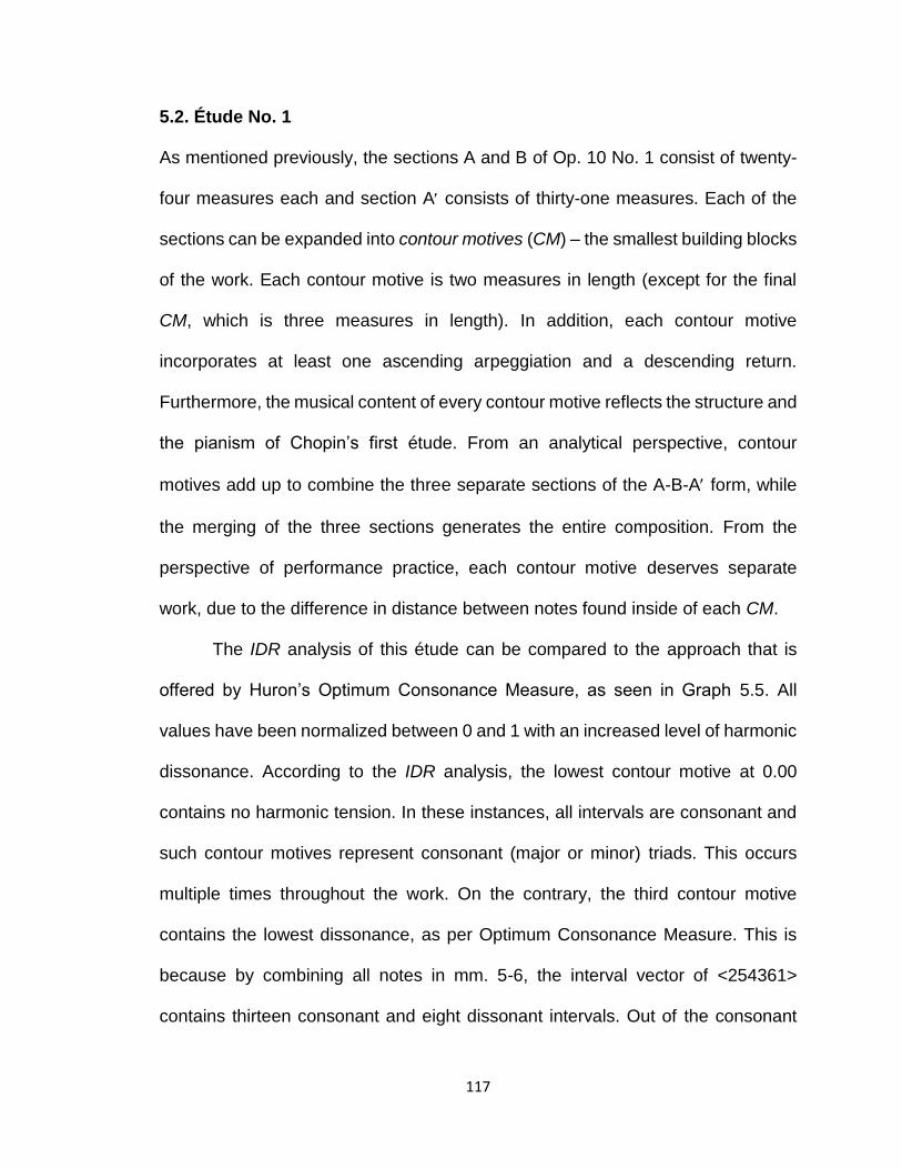
117

5.2. Étude No. 1

As mentioned previously, the sections A and B of Op. 10 No. 1 consist of twenty-

four measures each and section A consists of thirty-one measures. Each of the

sections can be expanded into contour motives (CM) – the smallest building blocks

of the work. Each contour motive is two measures in length (except for the final

CM, which is three measures in length). In addition, each contour motive

incorporates at least one ascending arpeggiation and a descending return.

Furthermore, the musical content of every contour motive reflects the structure and

the pianism of Chopin’s first étude. From an analytical perspective, contour

motives add up to combine the three separate sections of the A-B-A form, while

the merging of the three sections generates the entire composition. From the

perspective of performance practice, each contour motive deserves separate

work, due to the difference in distance between notes found inside of each CM.

The IDR analysis of this étude can be compared to the approach that is

offered by Huron’s Optimum Consonance Measure, as seen in Graph 5.5. All

values have been normalized between 0 and 1 with an increased level of harmonic

dissonance. According to the IDR analysis, the lowest contour motive at 0.00

contains no harmonic tension. In these instances, all intervals are consonant and

such contour motives represent consonant (major or minor) triads. This occurs

multiple times throughout the work. On the contrary, the third contour motive

contains the lowest dissonance, as per Optimum Consonance Measure. This is

because by combining all notes in mm. 5-6, the interval vector of <254361>

contains thirteen consonant and eight dissonant intervals. Out of the consonant

118

intervals, six of these are perfect fourths and perfect fifths and this particular

interval-class contains the highest effect on the overall increase in consonance.

According to the IDR, the highest dissonance in this étude is CM32, where 34.04%

of the interval-classes are dissonant. Based on Optimum Consonance Measure

calculations CM11 (mm. 21-22) and CM17 (mm. 33-34) have the highest

dissonance. This occurs because the pitches in mm. 21-22 and in mm. 33-34

generate interval-class vectors (<322332> and <122212>) with predominance of

dissonance intervals.

Graph 5.5: Comparison of IDR and Optimum Consonance Measure in Étude Op. 10 No. 1.

Some other interesting points of comparison between the IDR and Optimum

Consonance Measure can be seen in CM6, CM22, and CM30. CM6 contains the

juxtaposition of F major and F♯ diminished harmonies. While dissonance is evident

and is reflected in the Optimum Consonance Measure analysis, the harmonic

subdivision of each sixteenth beat nevertheless produces a series of consonant

interval-classes, which is why the IDR of this motive is 0.00%. The generated

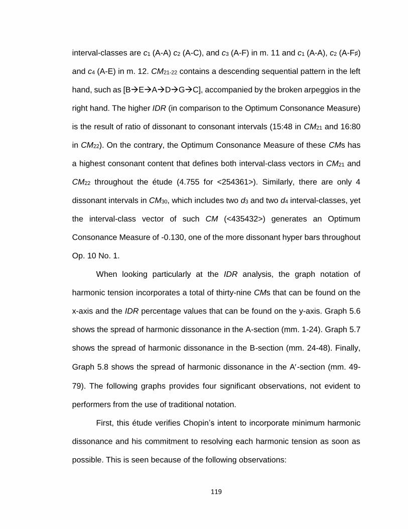
119

interval-classes are c1 (A-A) c2 (A-C), and c3 (A-F) in m. 11 and c1 (A-A), c2 (A-F♯)

and c4 (A-E) in m. 12. CM21-22 contains a descending sequential pattern in the left

hand, such as [BEADGC], accompanied by the broken arpeggios in the

right hand. The higher IDR (in comparison to the Optimum Consonance Measure)

is the result of ratio of dissonant to consonant intervals (15:48 in CM21 and 16:80

in CM22). On the contrary, the Optimum Consonance Measure of these CMs has

a highest consonant content that defines both interval-class vectors in CM21 and

CM22 throughout the étude (4.755 for <254361>). Similarly, there are only 4

dissonant intervals in CM30, which includes two d3 and two d4 interval-classes, yet

the interval-class vector of such CM (<435432>) generates an Optimum

Consonance Measure of -0.130, one of the more dissonant hyper bars throughout

Op. 10 No. 1.

When looking particularly at the IDR analysis, the graph notation of

harmonic tension incorporates a total of thirty-nine CMs that can be found on the

x-axis and the IDR percentage values that can be found on the y-axis. Graph 5.6

shows the spread of harmonic dissonance in the A-section (mm. 1-24). Graph 5.7

shows the spread of harmonic dissonance in the B-section (mm. 24-48). Finally,

Graph 5.8 shows the spread of harmonic dissonance in the A-section (mm. 49-

79). The following graphs provides four significant observations, not evident to

performers from the use of traditional notation.

First, this étude verifies Chopin’s intent to incorporate minimum harmonic

dissonance and his commitment to resolving each harmonic tension as soon as

possible. This is seen because of the following observations:

120

a) Twelve of thirty-nine CMs (≈31% of the entire work) incorporate perfect

harmonic consonance.

b) Each increase in harmonic tension is typically followed by an immediate

decrease in harmonic tension. This occurs fourteen times throughout the

work, while an increase in harmonic tension is followed by another increase

only three times (once in the A-section, once in the B-section, and once in

the A-section). While dissonance is essential in the arpeggiated sequences

of Chopin’s compositional approach, the composer is not interested in

prolonging it.

Graph 5.6: IDR of Étude Op. 10 No. 1, mm. 1-24.

121



Second, Chopin incorporates varied use of harmonic dissonance, ranging

between 4.26% and 34.04%, which is found in the étude’s twenty-seven CMs,

where the IDR is greater than 0.00%. Some IDR rates are identical. For instance,

122

CM1 through CM5 are identical to CM25 through CM29. This occurs because

sections A and A share the same opening harmonic cycle (a general

characterization of ternary form) with the turning point occurring at CM26.227 On

the contrary, CM14, CM15, and CM16 have no associations to each other from the

perspective of musical form, and while their IDR is identical at 14.89%, their

respective construction is not. The construction of the three CMs can be compared

through modicv. The ratio of CI to DI is 48:14 in CM14, CM15, and CM16. However,

a different modicv exists for seven (of the eight) different ic content, apart from the

stationary ic(d4).

a) modicv(CM14) = [48,0,8,24,0,14,0,0];

b) modicv(CM15) = [42,16,14,8,0,6,8,0];

c) modicv(CM16) = [40,8,24,8,0,14,0,0].

Third, the three largest dissonances in this étude are the only three IDR

values that are greater than 30%. All three dissonances resolve to perfect

harmonic consonance. In this work, there is:

a) One occurrence in the A-section, where CM11 with IDR of 31.91% resolves

to CM12, shown in Figure 5.5;

b) One occurrence in the B-section, where CM17 with IDR of 31.75% resolves

to CM18, shown in Figure 5.6;

c) One occurrence in the A-section, where CM32 with IDR of 34.04% resolves

to CM33, shown in Figure 5.7.

227 Richard Cohn, “Maximally Smooth Cycles, Hexatonic Systems, and the Analysis of Late-Romantic Triadic Progressions,” Music Analysis 15, no. 1 (March 1996), 15.

123




124

Fourth, it is evident that each of the three sections contains a wide range of

harmonic tension, yet each of the final cadences of sections A, B, and A ends on

perfect authentic cadence. According to the analysis the IDR of the A-section

fluctuates between 0.00% and 31.91% while cadencing on CM12, the IDR of the B-

section fluctuates between 0.00% and 31.75% while cadencing on CM24, and the

IDR of the A-section fluctuates between 0.00% and 34.04% while cadencing on

CM39. The IDR of CM12, CM24, and CM39 is 0.00%.

Chopin’s music provides theorists and musicologists with a variety of

compositional innovations in the development of tonal harmony.228 Harmonic

dissonance generated in Chopin’s compositions is a significant aspect of analysis

and performance.229 Each point of tension in Op. 10 No. 1 signifies a musical

climax that needs resolution and the graphical notation of harmonic dissonance

allows one to trace such tension through the étude.

5.3. Étude No. 2

The use of chromaticism in Op. 10 No. 2 allows Chopin to generate both vertical

and horizontal dissonance. The vertical dissonance is achieved through rhythm,

since the performer is required to hold the left hand’s bass voice and right hand’s

inner voices, both represented with eighth notes, at the time when the main melody

in the right hand ascends and descends in chromatic motion, represented with

228 Eugene Narmour, “Melodic Structuring of Harmonic Dissonance: A Method for Analyzing Chopin’s Contribution to the Development of Harmony” in Jim Samson, Chopin Studies, Volume I, Cambridge University Press, 1988. 229 James S. Walker and Gary W. Don, Mathematics and Music: Composition, Perception, and Performance. CRC Press, 2014.

125

sixteenth notes. The horizontal dissonance is achieved through constant half-step

perpetuum mobile motion. While there are instances, in which Chopin incorporates

alternate melodic intervals in the right hand, each note in the main melody is either

preceded or proceeded by its half-step neighbor at all times. The employment of

different levels of musical tension throughout the étude allows Chopin to move

between two or more harmonic structures. The use of dissonance likewise shows

Chopin’s modified harmonic paths, which are generated through multiple turning

points.

As seen previously, Huron’s Optimum Consonance Measure looks at the

aggregate consonance values, combining pitches into a multiple interval-class

vector. Due to the large amount of chromaticism in the second étude, such an

approach to analyzing dissonance in each measure will result in interval-class

vectors, generated from all possible pitch-classes. Such occurrence exists in the

very first measure of the work, generating an interval-class vector of <12 12 12 12

12 6>. However, Huron’s interval-class ranking can be applied to the IDR of each

measure, as seen in Graph 5.9. This creates a comparison of weighted interval-

classes (as seen in Huron’s Optimum Consonance Measure) and non-weighted

interval-classes (as seen in IDR). As seen from the analysis, the most consonant

harmony is A major, located at the very last measure of the work.

The IDR analysis is helpful for the analysis of harmonic dissonance based

on each measure, where the IDR is normalized between the values of 0 and 1 with

0 being equivalent to a perfect harmonic consonance. This type of analysis

presents three unique observations. First, the maxima IDR value in the graph of

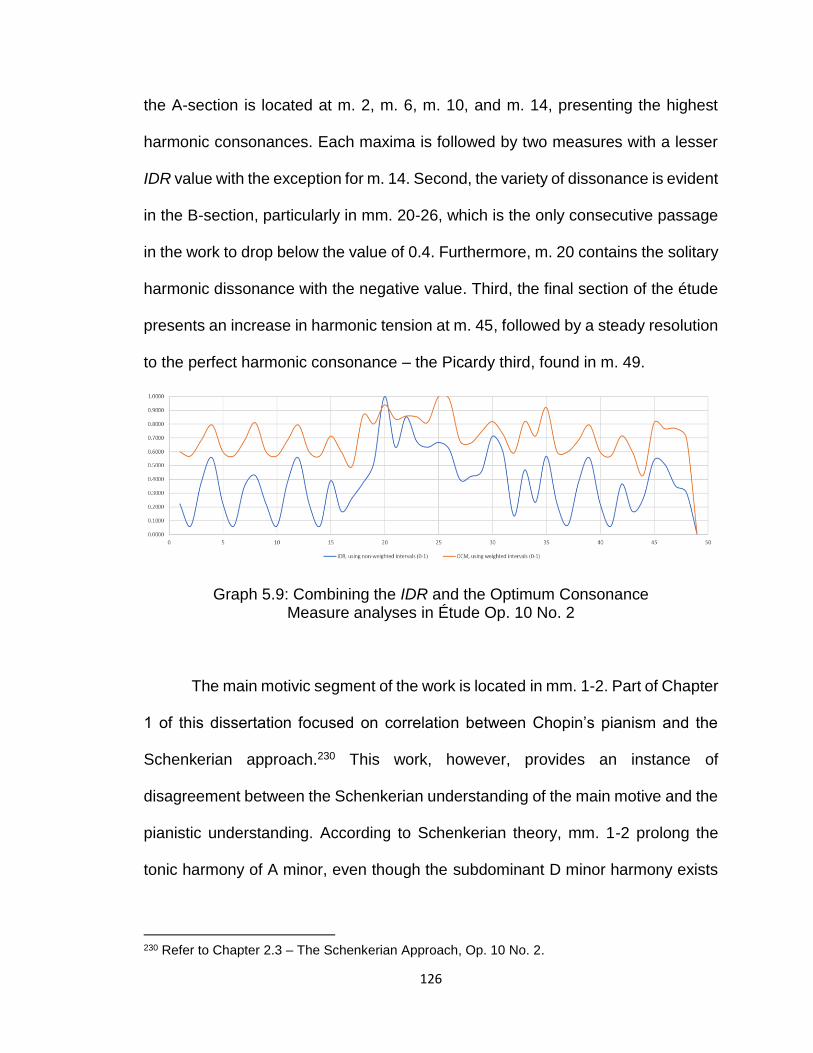
126

the A-section is located at m. 2, m. 6, m. 10, and m. 14, presenting the highest

harmonic consonances. Each maxima is followed by two measures with a lesser

IDR value with the exception for m. 14. Second, the variety of dissonance is evident

in the B-section, particularly in mm. 20-26, which is the only consecutive passage

in the work to drop below the value of 0.4. Furthermore, m. 20 contains the solitary

harmonic dissonance with the negative value. Third, the final section of the étude

presents an increase in harmonic tension at m. 45, followed by a steady resolution

to the perfect harmonic consonance – the Picardy third, found in m. 49.

Graph 5.9: Combining the IDR and the Optimum Consonance Measure analyses in Étude Op. 10 No. 2

The main motivic segment of the work is located in mm. 1-2. Part of Chapter

1 of this dissertation focused on correlation between Chopin’s pianism and the

Schenkerian approach.230 This work, however, provides an instance of

disagreement between the Schenkerian understanding of the main motive and the

pianistic understanding. According to Schenkerian theory, mm. 1-2 prolong the

tonic harmony of A minor, even though the subdominant D minor harmony exists

230 Refer to Chapter 2.3 – The Schenkerian Approach, Op. 10 No. 2.

127

in the second half of the first measure. On the other hand, based on the

performance practice of this étude, the D minor harmony cannot be ignored.231

Since dissonance governs the main character of this work and since the way in

which Chopin utilizes chromaticism creates multiple technical complexities, a

pianist needs to apply extra importance on consonant harmonies, and the D minor

harmony on beat 9 of m. 1 is one of the examples of perfect harmonic consonance.

A unique characteristic of this étude is the emphasis that Chopin puts on mm. 1-2

in the A and A sections. Table 5.5 shows the IDR analysis of mm. 1-2. This is a

highly consonant motive, where ic(d4) is the prime source of dissonance.

Table 5.5: The IDR analysis of Chopin’s Étude Op. 10 No. 2, mm. 1-2.

ic(c1) of m. 1-2 17/114 (14.91%)

ic(c2) of m. 1-2 27/114 (23.68%)

ic(c3) of m. 1-2 29/114 (25.44%)

ic(c4) of m. 1-2 32/114 (28.07%)

ic(d1) of m. 1-2 1/114 (0.88%)

ic(d2) of m. 1-2 2/114 (1.75%)

ic(d3) of m. 1-2 0/114 (0.00%)

ic(d4) of m. 1-2 6/114 (5.26%)


IDR% 7.89%

231 Kenneth Hamilton, After the Golden Age: Romantic Pianism and Modern Performance (Oxford: Oxford University Press, 2008), 69.

128

All seven phrases of both sections in the second étude begin with an

identical motive. Furthermore, the motive is responsible for generating multiple

harmonic turning points. The A-section of Op 10 No. 2 (mm. 1-17) contains three

small phrases of four measures (mm. 1-4), (mm. 5-8), and (mm. 9-12), as well as

one phrase of five measures (mm. 13-17). The A-section of Op. 10 No. 2 (mm.

36-49) contains one phrase of four measures (mm. 36-39) and two phrases of five

measures (40-44) and (45-49). The seven phrases with identical motives generate

six unique IDR rates, which are shown in Graph 5.10.232 Based on the IDR

analysis, both the A and A sections begin with the most harmonically dissonant

phrases and end with most harmonically consonant phrases. This is unlike Op. 10

No. 1, where the initial contour motives of the opening and the ending sections are

perfect harmonic consonances. Finally, it is important to note that while the second

étude resolves on tonic harmony of A major, the most consonant motive,

nevertheless, is the penultimate.

Graph 5.10: The IDR analysis of all seven phrases in Étude Op. 10 No. 2 with identical opening motive at mm. 1-2.

232 The music material found in mm. 1-4 and 9-12 is identical.

0.00%

5.00%

10.00%

15.00%

20.00%

mot. A1 mot. A2 mot. A3 mot. A4 mot. A5 mot. A6 mot. A7

129

5.4. Étude No. 3

The third étude does not carry any contour motive or unique motivic thematic idea,

on which the piece is based. The opening two measures of Op. 10 No. 3 initiate

merely two other phrases in m. 9 and m. 62 (the start of A-section). Instead,

Chopin uses multiple levels of dissonance in several passages of the work. The A-

section spans until the cadence on the start of m. 21 and can be subdivided into

three phrases. These are mm. 1-5, mm. 6-13, and mm. 14-21. The B-section can

be subdivided into four phrases. The first phrase spans until the subdominant

harmony of A major at the start of m. 30. The second phrase continues until the E♯

fully-diminished seventh chord at the start of m. 38. The third phrase extends until

the B major harmony at the beginning of m. 46. The fourth phrase spans until the

half cadence at the start of m. 54. The passage in m. 54-61 serves as a transition

into the A-section. Comparable to Op. 10 No. 2, Chopin’s A-section is significantly

shorter than the opening section, based on identical thematic material, and

consists of two phrases, found in mm. 62-66 and mm. 67-77.

The comparison between the Huron’s Optimum Consonance Measure and

the IDR can be used to understand the harmonic makeup of the composition.

Based on the harmonic and the Schenkerian analyses of this étude, the harmony

of the opening phrase (mm. 1-5) consists of alternating tonic and dominant seventh

chords. The Optimum Consonance Measure of m. 1 is 2.459, consisting of pitches

D♯, E, F♯, G♯, A, and B with an interval-class vector of <233241>. The Optimum

Consonance Measure of m. 2 is identical to m. 1 with identical pitches and interval-

class vector. The Optimum Consonance Measure presents the same consonance

130

results in the opening of the first phrase. Such metric allows one to trace the

harmonic plan of mm. 1-2 in terms of dissonance level, since m. 1 utilizes tonic

moving towards the dominant and m. 2 returns the dominant back to the tonic. The

third measure of the étude employs pitches C♯, D♯, E, G♯, A, and B with an interval-

class vector of <232341> and Optimum Consonance value of 2.251. In this

instance, however, C♯ is used in lieu of F♯. Measures 4 and 5 use pitches C♯, D♯,

E, F♯, G♯, A, and B, generating an interval-class vector of <254361> and Optimum

Consonance value of 4.755. The first five measures of the étude generate three

Optimum Consonance values. On the contrary, the IDR generates four unique

values because of consideration for repeated pitches as well as inclusion of

unisons, octaves, and equivalent intervals. The average Optimum Consonance

value of each eighth harmonic slices can also be compared to the IDR, as shown

in Graph 5.11.

Graph 5.11: The IDR and the Optimum Consonance Measure analyses of Chopin’s Étude Op. 10 No. 3.

Similar to Op. 10 No. 2, certain passages in the third étude contain hidden

chromaticism patterns in each measure and will therefore generate complex

interval-class vectors. This can be seen in mm. 46-51. The Optimum Consonance

131

Measure of m. 46, m. 48, and m. 50 is 1.404 with the interval-class vector of

<448444>, consolidating eight of the possible twelve pitches. The Optimum

Consonance Measure of m. 47, m. 49, and m. 51 is -0.198 with the interval-class

vector of <12 12 12 12 12 6>, consolidating all twelve pitches. This means that

according to the Optimum Consonance Measure, m. 46, m. 48, and m. 50 are

slightly consonant (as 1.404 > 0), while m. 47, m. 49, and m. 51 are slightly

dissonant (as -0.198 < 0).233 This passage contains a descending series of

harmonic alternating sixths (both major and minor) and diminished sevenths.

A disparity in analyses based on IDR and Optimum Consonance Measure

can be seen in mm. 20-30 and mm. 70-77. This occurs because of certain Huron’s

interval ranking indexes that generate a high level of harmonic dissonance. For

instance, m. 22 has an IDR of 16.67% and only contains four dissonant intervals:

A♯-E, F♯-E, E-A♯, and B-C♯. Two of these are ic6 on the standard interval-class

vector with index value of -0.453 and two of these are ic2 on the standard interval-

class vector with index value of -0.582. By applying Huron’s index values that

generate ranking for interval-classes, the Optimum Consonance Measure of m. 22

is 1.4295, which is 0.7709 on a 0-1 scale and contains less consonance than

similar passage, according to the IDR.

This étude is an example of Chopin’s ability to create a mix of unstable and

unbalanced harmonies. The IDR analysis of Op. 10 No. 3 reveals that Chopin uses

gradual harmonic dissonance to enhance musical tension towards the dissonant

nucleus of the B-section, found at mm. 38-42. This passage, constructed from a

233 David Huron, “Interval-Class Content in Equally Tempered Pitch-Class Sets: Common Scales Exhibit Optimum Tonal Consonance,” Music Perception 11, no. 3 (Spring 1994): 294.

132

series of fully-diminished chords, contains the musical climax of the entire work

and requires resolution, which occurs on the B major harmony in the first beat of

bar 42. Graph 5.12 shows the increase in harmonic dissonance, as one reaches

mm. 38-42, as well as an increase in harmonic consonance, as the work comes to

a close.

Graph 5.12: The IDR analysis of all phrases in Étude Op. 10 No. 3.

The three phrases of the A-section range between the IDR of 15.21% and

18.52%. Chopin makes sure to resolve any dissonant components of harmony.

Each phrase of the A-section cadences on the tonic of E major. The B-section

contains a larger variety of harmonic dissonance, ranging from 12.89% to 47.92%.

In addition, the four cadential endings of each phrase never reach the harmony of

E major. The third phrase of the B-section is of most interest. The phrase can be

bifurcated into two subphrases. The opening of the third phrase is highly dissonant

with the IDR of 47.92%. On the other hand, the closure of the phrase is highly

consonant with the IDR of 12.89%, making it the most consonant passage in the

étude.

133

The interpretation that one builds in the reading of a work is an essential

component in studies of the performance practice. In the case of Op. 10 Nos. 1

and 2, the deviation in interpretation is not very large and the melodic motion is

self-evident for majority of pianists. On the contrary, Op. 10 No. 3 differs in its

departure from technical virtuosity and places emphasis on the poetic nature of its

melody. The deviations in tempo, dynamics, and pedaling are some of the

components on which pianists work to create an appropriate interpretation in this

étude. Knowledge and familiarity with harmonic dissonance can allow pianists to

incorporate such information into their own interpretations. This can be seen in

performance analysis of mm. 38-54 of Maurizio Pollini, Lang Lang, and Valentina

Lisitsa.234

The interpretational differences occur in three passages: mm. 38-42 and

mm. 46-54, both of which contain a series of fully-diminished seventh chords,

resolving on B major harmony, as well as mm. 42-46, which serves as the transition

between the two dissonant passages.

Pollini establishes three groups in mm. 38-42, based on Chopin’s slurring

recommendations, and stays very close to what the score suggests. Pollini likewise

groups the passage in mm. 46-54, based on slight dynamic accents on the first

beat of every measure. Lang Lang abruptly increases the tempo and the volume

in mm. 38-42 and makes sure to emphasize the final B major harmony.

Furthermore, Lang Lang continues to increase the tempo in mm. 42 and 46,

234 Maurizio Pollini, Chopin Études, Deutsche Grammophon 00289-477-8423, 1985. Lang Lang, The Chopin Album, Sony Classical 88725449602, 2012. Valentina Lisitsa, Chopin: 12 Études Op. 10, Decca, 2014.

134

specifically on the consonant harmonic alterations of [D-B] and [A-F♯] in m. 42.

Finally, Lang Lang gradually decreases the tempo in the last section of the

passage. It is important to note that every chord is emphasized, making the

harmonic dissonance very apparent. Similarly to Lang Lang, Lisitsa increases the

tempo and crescendos towards the B major harmony in m. 42. Lisitsa employs

aberrant pedaling in mm. 46-52 to emphasize dissonance that is created between

alternating sevenths and sixths intervals before suddenly decreasing and returning

to the original tempo in in m. 53. In all performances, such dissonant passages are

open to pianistic interpretation and can be understood musically in multiple ways.

5.5. Étude No. 4

The fourth étude is one of the most harmonically complex works in Op. 10. The

high level of dissonance in this work depends on Chopin’s consolidation of

arpeggiation, chromaticism, and linear patterns, which can be noticed in mm. 28-

34. Beats 1, 5, 9, and 13 (of 16) in mm. 28-29 consist of harmonic triads or seventh

chords, while the melody in the same passage consists of ascends and descends

by a half (chromatic) or a whole step. On the contrary, the melodic motion in the

inner voices of mm. 32-33 is consonant moving downward by harmonic major or

minor thirds.

Another distinct characteristic of this study is Chopin’s subtle differences in

alternating thematic material between section A and A. This can be seen in m. 8

(Figure 5.8) and m. 58 (Figure 5.9). In the A-section, a series of half-step patterns

on m. 8, represented by the eighth notes, is to be held in the inner voice of the right

135

hand while the main melody continues in perpetual motion, represented by the

sixteenth notes. This creates an extra layer of harmonic dissonance, overlapping

each of the sixteenth notes with the right hand’s main melody and the left hand’s

bass support. On the contrary, Chopin avoids the inner voice in m. 58 of the A-

section and instead focuses on a two-voice contrary motion. The lack of secondary

melody decreases the IDR from 18.33% (m. 8) to 15.91% (m. 58).



Graph 5.13 shows the comparison between the IDR and Huron’s Optimum

Consonance Measure analyses. The highest dissonance in both analyses occurs

in m. 39-40. In this passage, both right and left hands create a descending two-

part harmony using broken seventh chords in the lower melody and linear pattern

136

with chromatic ascents in the main melody. A disparity in both analyses occurs at

the end of A-section, where the Optimum Consonance Measure is higher than the

IDR. This occurs because of large amount of d1 interval-classes on the modified

interval-class vector, equivalent to ic1 on the traditional interval-class vector in mm.

71-79. Out of 242 total intervals in this passage, 65 are dissonant and 76 belong

to class c1, which Huron’s Optimum Consonance Measure does not rank. Out of

65 harmonic dissonances, 19 of these (29.23% of total dissonance) belong to d1

class and 27 of these (41.53%) belong to the d2 class. Huron’s index values for ic1

and ic2 on traditional interval-class vector are -1.428 and -0.582. Such high

dissonance occurrence is the reason why this passage is ranked highly dissonant

according to the Optimum Consonance Value analysis.

Graph 5.13: The IDR and the Optimum Consonance Measure analyses of Chopin’s Étude Op. 10 No. 4.

137

CHAPTER 6. CONCLUSION

The notion of consonance and dissonance plays a prominent role in Western

music. The generation of tension and its resolution is one of the largest

fundamental principles that exists in tonal literature. Consonance and dissonance

in each musical work provides a degree of contrast and ‘polarity’, which can be

viewed from the stance of cognitivism, physicalism, and immanentism.235 In

Chopin's music, harmonic dissonance can be interpreted as a musical function that

requires detailed analysis and examination. It is up to each individual composer to

enhance one’s composition by producing areas of tension and by deciding how

such dissonant regions will be finalized from melodic and harmonic viewpoints.

Mathematically, the methods for computing for musical tension vary,

depending on goals that one wishes to achieve by such calculations. The primary

focus of IDR research is to compute the level of harmonic dissonance based on

verticalities from the standpoint of interval-classes. In addition to the dissonance

rates, the proposed methodology likewise generates data for the analytic

investigation of intervallic structure. Each verticality can be expressed as a ratio of

consonant and dissonant intervals and a series of such verticalities generate the

harmonic and melodic formulae in a composition. The dissonance in a musical

work that derives from such harmony and melody is an artistic component, which

a pianist must execute in a performance. Therefore, the connection between

pianism, Schenkerian analysis, and computation of dissonance is a vital aspect to

consider when understanding a work on both artistic and analytical levels.

235 Norman Cazden, "The Definition of Consonance and Dissonance," International Review of the Aesthetics and Sociology of Music 11, no. 2 (December 1980), 124.

138

The intervallic makeup of a musical work relates to several features of its

style and genre. In the case of Chopin’s music (and particularly in the case of

Chopin’s études), such features are purely pianistic.236 Furthermore, the unique

interval-classes generate harmonies, which in turn, produce chordal progressions

and harmonic regions that Chopin arranges in a unique way. The details of such

arrangement constitute a significant component of Chopin’s compositional

language and lead to his idiomatic treatment of harmonic dissonance. Likewise,

the aspects of the piano technique are significant to take into consideration in

Études Op. 10 Nos. 1-4, since they also influence the harmonic path that the

composer selects. A series of verticalities in the four études provides one with a

data set for the evaluation of harmonic tension and intervallic distribution.

In Op. 10 No. 1, 47.87% of all interval-classes are perfect unisons and

octaves, most of which are found in the left hand. The IDR analysis reveals that

these interval-classes assist with producing a low dissonance ratio throughout the

étude. Analytically, such intervals typically double the chordal factors of the major

and minor triads, on which the work is based. Pianistically, the octaves in the left

hand constitute a main melody that the right hand’s arpeggiations harmonize.237 In

addition, supplementary octaves are produced when verticalities in the left hand’s

melody correspond with the equivalent chordal factor in each right hand’s

236 It is important to remember that Chopin himself was a pianist and pedagogue. Therefore, while many of his pieces are complex from the standpoints of artistry, musicianship, and technique, Chopin’s works are nevertheless pianistically comfortable. Irena Poniatowska, Fryderyk Chopin: The Man and his Music (Warsaw: Multico Oficyna Wydawnicza. 2010), 125. 237 The primary thematic material is in the right hand’s arpeggiation. However, the right hand does not generate a melody. On the contrary, the left hand does not carry technical difficulties, yet produces a melody that outlines the form of each of the three sections in the étude.

139

arpeggio. Since the octaves and equivalent intervals constitute almost half of the

composition, it is important to highlight them pianistically.238 There are multiple

methodologies to do so, one of which is employing accentuation, specifically on

linear patterns and fully established phrases.239

When it comes to comparing all possible contour motives in Op. 10 No. 1,

only 14.14% of intervals are dissonant, with thirty-seven out of thirty-nine IDR

values below 30%. This occurs because the arpeggiation patterns in this étude

generate low amounts of dissonance, given the surplus of two-note dyads that

arise between the first, the third, and the fifth chordal factors. Pianistically

speaking, such phenomenon is only possible in predominantly triadic music, as

shown in this étude, since the primary purpose of this work is to generate a series

of practical components for enhancing arpeggio playing. Another intersection

between the IDR and Chopin’s compositional approach can be seen in purely

consonant contour motives, occurring in twelve separate passages, combining for

a total of twenty-five measures of pure consonant verticalities.

From a pianistic standpoint, Op. 10 No. 1 is an appropriate work for the

inclusion of these purely consonant passages, as Chopin is following a

compositional plan related to a specific technique, alternating ascending and

descending arpeggios. On the contrary, employing only unisons, thirds, fourths,

fifths, sixths, octaves, and equivalent intervals may be considered too simplistic for

Romantic era music in general, particularly for a work that is meant to provide

238 In Chopin’s compositional output, there are several études that specifically focus on a particular interval. 239 For pianistic interpretation (both technical and artistic) of Études Op. 10, refer to Alfred Cortot, Chopin: 12 Studies Op. 10. Paris: Editions Salabert, 1915.

140

challenges and complications for a pianist’s sense of artistry.240 In Chopin’s Op.

10, Op. 25, and Trois Nouvelles Études, Op. 10 No. 5 (Black Key) and Op. 25 No.

12 (Ocean) are the only other works, in which the composer incorporates pure

arpeggiation for a substantial passage in a work.241 There are likewise three études

that emphasize specific intervals and, therefore, are based on subsets of

arpeggiation. This can be in Op. 25 No. 6, where a pianist must focus on thirds,

Op. 25 No. 8, where a pianist must focus on sixths, and Op. 25 No. 10, where a

pianist must focus on octaves. Such a compositional layout is not stylistic in more

artistically-inclined Romantic compositions, or in works that are based on

alternative pianistic techniques.

A musical composition can be dissected analytically, historically, or

pianistically.242 In particular, music analysis allows one to separate and view the

structural components of any work. From the perspective of theory, Schenkerian

analysis presents a series of compositional rules that occur in the melody,

harmony, and counterpoint. Furthermore, Schenkerian analysis defines and

denotes a series of structural components with notated elaborations. Schenkerian

prolongations reveal how various passages in a musical piece function and

associate with one another. As pianistic techniques serve as the primary

240 Irena Poniatowska, Fryderyk Chopin: The Man and his Music (Warsaw: Multico Oficyna

Wydawnicza, 2010), 120. 241 While the arpeggiation is used in both Op. 10 No. 5 and Op. 25 No. 12, the compositional strategy varies. 242 This is likewise known as holistic musical analysis. For more information on such musical evaluation, refer to: Daniil Zavlunov, "The 'tselostnyi analiz' (holistic analysis) of Zuckerman and Mazel," Music Theory Online 20, no. 3 (2014). Hugh Aitken, The Piece as a Whole: Studies in Holistic Musical Analysis. Contributions to the Study of Music and Dance (Westport, CN: Praeger, 1997).

141

foundations of Chopin’s études, Schenkerian analysis can represent and graph

these components in analytical terms. In addition to pianism, the Schenkerian

analysis can assist with identification of dissonance and the IDR application can

be beneficial for mathematically calculating and classifying various dissonance

levels.

During Chopin’s artistic period, the notion of tonality was the accustomed

compositional tradition. Nonetheless, components such as chromaticism produce

aspects of tonal ambiguities, as seen in Op. 10 No. 2. Chromaticism is present in

the opening section of the work in the right hand’s primary voice in mm. 1-17.

Throughout this passage, the level of vertical dissonance fluctuates between

12.5% and 31.25%. Whereas the inclusion of chromatic harmony produces higher

levels of tonal tension, the IDR calculations allow one to see and compare various

harmonically dissonant regions in the score regardless of their degree of

chromaticism. For instance, the highest harmonic tension in the A-section occurs

in m. 4, m. 8, and m. 12. These measures contain half cadences that generate

tension and seek for respective resolutions into m. 5, m. 9, and m. 13. Pianistically,

the opening three primary sub-phrases of mm. 1-17 are mm. 1-4, mm. 5-8, and

mm. 9-12, each of which begins with identical thematic material.

In this instance through the use of technique of diminution, Schenkerian

analysis represents such subphrases as a series of I-V progressions, each with

identical half cadence that resolves to the tonic, generating three consecutive

identical reoccurrences. By analyzing harmonic dissonance, it is evident that the

most discordant regions in the A-section are the harmonies that seek to return to

142

tonic. As the analytical theory behind the construction of this section becomes

relatively evident, the pianistic comprehension is not, since there are numerous

interpretive and subjective aspects that an artist must decide for oneself.243 This is

because the pianistic facets, such as rubato, the level of crescendo, accentuation,

and the use of sustaining pedal must be carefully planned for a well-built artistic

interpretation.

Another connection between pianism, Schenkerian analysis, and the

dissonance range can be seen in the main melody of Étude Op. 10 No. 2. From

the standpoint of pianism, this work has three layers: the main melody in the right

hand, the bass accompaniment in the left hand, and the subordinate inner voices

played by the left and the right hands. For an accurate performance, it is crucial

that the main melody is emphasized in a smooth and graceful manner, while the

bass and the inner voices are employed as harmonic support for the primary

voice.244 Analytically, the chromatic passages range between pitch A (^1) and the

apex – pitch F (^6). Each hyperbar that initializes every subphrase in the A-section

of Op. 10 No. 2 contains an ascending and a descending chromatic passage.

Schenkerian analysis emphasizes the lowest and the highest pitches of these

melodies.

From the perspective of dissonance, the amount of harmonic tension

decreases as the chromatic line ascends, while the amount of harmonic tension

increases as the chromatic line descends. This generates an interesting

243 Alfred Cortot, Chopin: 12 Studies Op. 10. (Paris: Editions Salabert, 1915), 15. 244 In certain passages, some pianists may choose to emphasize parts of the bass accompaniment or subordinate voices for the purpose of musical contrast.

143

interpretive situation, since a crescendo occurs with the decrease in vertical

dissonance and a diminuendo occurs with the increase of vertical dissonance.

While employing chromaticism in Op. 10 No. 2, Chopin does not highlight any

particular harmonic interval-classes. On the contrary, Op. 25 No. 5, nicknamed

(Wrong Note) uses a large amount of melodic minor seconds, generating a high

level of melodic dissonance.

Another interaction between the combined functionality of pianism,

Schenkerian analysis, and IDR can be seen in the meaning of harmony in Étude

Op. 10 No. 3. The most dissonant section of the work, found in mm. 38-41 is of

most interested here.245 With an IDR of 47.92%, this passage is the only excerpt

in the work to contain such a large amount of dissonance, due to a series of fully-

diminished seventh chords. Pianistically and analytically speaking, Chopin

deviates from his traditional use of harmony and chooses to integrate a prominent

vertically dissonant section. The high IDR rate is significant both in terms of

performance practice and music analysis. While no specific emphasis is needed

to highlight a series of dissonant progressions, there are multiple interpretations

how such passage should be played; in the history of performance practice, there

have been many interpretations of this excerpt.

However, the amount of dissonance is not the only noteworthy musical

component of this passage. Additionally, its resolution is likewise significant, as

mm. 38-42 resolve to the dominant region of B Major. A typical phrase at its most

simple level can be notated as I-V-I, generating a tonic region, a dominant region,

245 This is shown in Figure 2.22.

144

and a return to tonic region. In the A-section, the dominant harmony serves the

role of a dissonant harmonic region, as E major moves to its (dissonant) dominant

B major, which seeks resolution by returning to the tonic E major, hence generating

a I-V-I progression. On the contrary, the symbolism of the B major harmony in m.

42 relies on the fact that it serves as a stable region, employed as an area for

resolution of mm. 38-41, rather than as a traditional dominant harmonic region that

would seek such resolution. The IDR assists the Schenkerian understanding of

such analytical component and it is up to the pianist to produce an interpretation

that would fulfill Chopin’s approach to dealing with the B major harmonic region.

For music theorists, the IDR serves as an analytical technique that can

examine and evaluate harmonic dissonance of a piece, based on the modified

interval-vector, construed from eight interval-classes.246 The IDR can be used to

make comparisons between different stylistic periods of a composer and between

different composers of the same stylistic era. For instance, the IDR can compare

the amount of harmonic dissonance that Beethoven uses in his early period,

middle period, and late period sonatas. Another example of hypothetical IDR

application can be seen in assessment and evaluation of harmonic dissonance in

romances of the same compositional period, such as of Cesar Cui and Nikolai

Rimsky-Korsakov.247 Finally, other works by Chopin can be tested for dissonance,

246 It is also important to note that the d4 interval-class can likewise be subdivided into multiple subgroups. 247 Stylistically, both composers were a part of the Mighty Five.

145

focusing on the relations and associations of interval-classes throughout the

works, both small and large-scale compositions.248

For pianists, the technique of IDR can be employed when shaping their own

interpretations in performances.249 For instance, a unique dissonant section can

be emphasized musically through dynamics and articulation. This leads to the

amalgamation of performance and analysis, allowing musicians to generate an

artistic reading of a work based on the extracted empirical data. Furthermore, the

IDR can provide an insight into dissonance levels in works, which were influenced

by historically earlier composers.

For instance, Scriabin, in his early compositional period, is inspired and

influenced by Chopin and, therefore, many of Scriabin’s early works reveal traces

of Chopin’s compositional approaches.250 The salient chromaticism in Chopin’s

Op. 10 No. 2 was seen previously in Figure 1.2. In contrast, the chromaticism in

Scriabin’s Op. 11 No. 2 is concealed between the primary melody and subordinary

thematic material, as shown in in mm. 7-9 of the A-section in Figure 6.1.251

248 For instance, the IDR can be used to calculate the harmonic dissonance of Chopin’s nocturnes or the four scherzi. 249 For more information on performance practice and the use of musical interpretation to shape dissonance, refer to: Clive Brown, Classical & Romantic Performing Practice 1750-1900 (Oxford: Oxford University Press, 2004). 250 Hwa-Young Lee, "Tradition and Innovation in the Twenty-Four Preludes, Opus 11 of Alexander Scriabin," DMA Monograph, University of Texas, 2006. 251 Nikita Mamedov and Robert Peck, “The Interval Dissonance Rate: An Analytical Look into

Chromaticism of Chopin’s Op. 10 No. 2 and Scriabin’s Op. 11 No. 2” in Proceedings of Bridges 2017 (Phoenix, AZ: Tessellations Publishing, 2017), 477.

146

Figure 6.1: Scriabin’s Op. 11 No. 2, mm. 7-9.252

Scriabin’s work contains evident traits of Chopinesque lyricism, even

though it incorporates different approaches to chromaticism and is tonally more

complex. Considering harmonic dissonance, Chopin uses 4.19% of tritones and

equivalent intervals, while Scriabin uses 10.58%. This is a significant percentile,

as the combined IDR of Scriabin’s Op. 11 No. 2 is 29.37%. On the contrary,

Chopin’s Op. 10 No. 2 utilizes 21.59% of unisons, octaves, and similar intervals –

a significant amount, due to the predominance of chromatic scalar passages.

Unlike Chopin’s étude, Scriabin’s Op. 11 No. 2 employs merely 9.08% of

octaves. It is evident that unlike Chopin, Scriabin makes sure to hide the chromatic

passages, concealing them with alternative harmonic dissonances. From a

pianistic standpoint, while both works carry many similarities, different

performative approaches must be taken. In Chopin’s Op. 10 No. 2, the chromatic

lines do not need to be emphasized and their clarity is evident nonetheless. On the

contrary, a performer is required to uncover and emphasize the chromatic

252 Alexander Scriabin, The Complete Preludes & Études for Pianoforte Solo (New York: Dover

Publications, 1973), 6

147

elaborations in Scriabin’s Op. 11 No. 2. Such artistic elements are essential for

pianists to notice and are prominent components of modern performance practice.

Western tonal music contains a repertoire of multiple styles and various

theoretical analyses have been applied to music literature of different epochs. One

of the ways to subdivide multiple centuries of compositions is by the concept of

tonality. Roman numeral analysis and Schenkerian analysis, which are based on

the principles of harmony and counterpoint, are two of the common methods to

look at music that contains a tonal center. The IDR can be applied to any tonal

piece that contains harmonic construction. By providing empirical data on how

dissonant a piece of music is harmonically, the IDR can be used to identify and

categorize patterns of dissonance and consonance in the music of various

composers.

148

BIBLIOGRAPHY

Agmon, Eytan. "The Bridges that Never Were: Schenker on the Contrapuntal Origin of the Triad and Seventh Chord." Music Theory Online 3, no. 1 (January 1997).

Aitken, Hugh. The Piece as a Whole: Studies in Holistic Musical Analysis. Contributions to the Study of Music and Dance. Westport, CN: Praeger. 1997.

Aranovsky, Mark. “Теория и Концепция Яворского.” [Eng: The Theory and the Conception of Yavorsky] Искуство Музыки: Теория и История 6 (2012): 41-60.

Beethoven, Ludwig Van. Klaviersonaten. Munich: G. Henle Verlag. 1980.

Bellman, Jonathan D. Chopin and his World. Princeton, NJ: Princeton University Press. 2017.

Bent, Ian. "Heinrich Schenker, Chopin and Domenico Scarlatti." Music Analysis 5, no. 3 (July 1986): 131-149.

Benward, Bruce, and Marilyn Saker. Music in Theory and Practice, Volume 2. New York: McGraw-Hill Companies. 2009.

Berezovsky, Boris. Chopin Études. Teldec 9031-73129-2. 1991.

Bortz, Yuri. “The Stylistic Foundation in the Etudes of Chopin, Scriabin, and Messiaen.” Master’s Thesis, University of Akron, 1997.

Brown, Clive. Classical & Romantic Performing Practice 1750-1900. Oxford: Oxford University Press. 2004.

Cadwallader, Allen, and David Gagné. Analysis of Tonal Music: A Schenkerian Approach. Oxford: Oxford University Press. 2011.

Caplin, William E. "Theories of Musical Rhythm in the Eighteenth and Nineteenth Centuries." In The Cambridge History of Western Music Theory, edited by Thomas Christensen, 657-694. Cambridge: Cambridge University Press. 2008.

Cazden, Norman. "The Definition of Consonance and Dissonance." International Review of the Aesthetics and Sociology of Music 11, no. 2 (December 1980): 123-168.

Chechlińska Zofia. "Szymanowska, Maria Agata." Oxford Music Online. Accessed January 12, 2018. http://www.oxfordmusiconline.com/subscriber/article/grove/music/27327.

Chopin, Frédéric. Douze Grandes Études. New York: Schirmer Inc. 1934.

Chopin, Frédéric. Études Op. 10. Leipzig: C. F. Peters. 1879.

149

Chopin, Frédéric. Études Op. 25. Leipzig: C. F. Peters. 1879.

Chopin, Frédéric, and Albert R. Parsons (ed.). Frederick Chopin's Works: Instructive Edition with Explanatory Remarks and Fingerings by Dr. Theodore Kullak. New York: Schirmer. 1880.

Clementi, Muzio. Gradus ad Parnassum. New York: Schirmer. 1908.

Cohn, Richard. "Maximally Smooth Cycles, Hexatonic Systems, and the Analysis of late-Romantic Triadic Progression." Music Analysis 15, no. 1 (March 1996): 9-40.

Cook, Nicholas. "Between Process and Product: Music and/as Performance." Music Theory Online 7, no. 2 (April 2001).

Cook, Nicholas. Beyond the Score: Music as Performance. Oxford: Oxford University Press. 2013.

Cortot, Alfred. Chopin: 12 Studies Op. 10. Paris: Editions Salabert, 1915.

Cramer, Johann Baptist. Studio per il Pianoforte. Leipzig: C. F. Peters. 1890.

Cross, Ian. “Music Science and Three Views.” Revue Belge de Musicologie / Belgisch Tijdschrift voor Muziekwetenschap 52 (1998): 207-214.

Czerny, Carl. Die Kunst Der Fingerfertigkeit. Frankfurt: C. F. Peters. 1950.

Czerny, Carl. School of Practical Composition, Volume I. London: Robert Cocks & Co., 1848.

De Clercq, Trevor. "Big Data, Big Question: A Closer Look at the Yale–Clasical Archives Corpus." Empirical Musicology Review 11, no.1 (2016): 59-68.

De Voto, Mark. "Some Aspects of Parallel Harmony in Debussy." In Liber Amicorum Isabelle Cazeaux: Symbols, Parallels and Discoveries in Her Honor, edited by Paul-Andru Bempechat, 459-485. Hillsdale, NY: Pendragon Press. 2002.

Dobrzański, Slawomir. “Maria Szymanowska and Fryderyk Chopin: Parallelism and Influence.” Polish Music Journal 5, no. 1 (Summer 2002): 1-15.

Downes, Stephen. Music and Decadence in European Modernism: The Case of Central and Eastern Europe. Cambridge: Cambridge University Press. 2010.

Drabkin, William. "Tritone." Groves Music Online. 2008. http://www.oxfordmusiconline.com/subscriber/article/grove/music/28403.

Eigeldinger, Jean-Jacques. Chopin: Pianist and Teacher as Seen by his Pupils. Cambridge: Cambridge University Press. 1986.

Fauvel, John, Flood, Raymond, and Robin Wilson. Music and Mathematics: From Pythagoras to Fractals. Oxford: Oxford University Press, 2010.

150

Fielden, Thomas. "Tempo Rubato." Music & Letters 23, no. 1 (April 1953): 150-152.

Forte, Allen and Steven E. Gilbert. Instructor's Manual for Introduction to Schenkerian Analysis. New York: W. W. Norton & Co. 1982.

Fulford, Tim. Literature, Science and Exploration in the Romantic Era: Bodies of Knowledge. Cambridge: Cambridge University Press. 2007.

Gamer, Carlton. "Some Combinational Resources of Equal-Tempered Systems." Journal of Music Theory 11, no. 1 (1967).

German, Franciszek. "Chopin and Mickiewicz." Rocznik Chopinowski 1 (1956): 227-253.

Godowsky, Leopold. Studien über die Etüden von Chopin. Berlin: Schlesinger. 1914.

Goldberg, Halina. Music in Chopin's Warsaw. Oxford: Oxford University Press. 2008.

Goldberg, Halina. The Age of Chopin: Interdisciplinary Inquiries. Bloomington, IN: Indiana University Press. 2004.

Hanson, Howard. Harmonic Materials of Modern Music: Resources of the Tempered Scale. New York: Appleton-Century-Crofts. 1960.

Heble, Ajay. Landing on the Wrong Note: Jazz, Dissonance, and Critical Practice. London: Routledge. 2000.

Hopkins, Charles. "Godowsky, Leopold." Oxford Music Online. Accessed December 15, 2017. http://www.oxfordmusiconline.com/subscriber/article/grove/music/11344.

Hoyt, Reed J. “Harmonic Process, Melodic Process, and Interpretive Aspects of Chopin’s Prelude in G Minor.” Indiana Theory Review 5, no. 3 (Spring 1982): 22-42.

Huron, David. “Interval-Class Content in Equally Tempered Pitch-Class Sets: Common Scales Exhibit Optimum Tonal Consonance.” Music Perception 11, no. 3 (Spring 1994): 289-305.

Hutchinson, W., and L. Knopoff. “The Acoustic Component of Western Consonance.” Interface 7 no. 1 (1978): 1-29.

Hutchinson, W., and L. Knopoff. “The Significance of the Acoustic Component of Consonance in Western Triads.” Journal of Musicological Research 3 (1979): 5-22.

Isaacson, Eric J. “Similarity of Interval-Class Content Between Pitch-Class Sets: The ICVSIM Relation.” Journal of Music Theory 34, no. 1 (Spring 1990): 1–18.

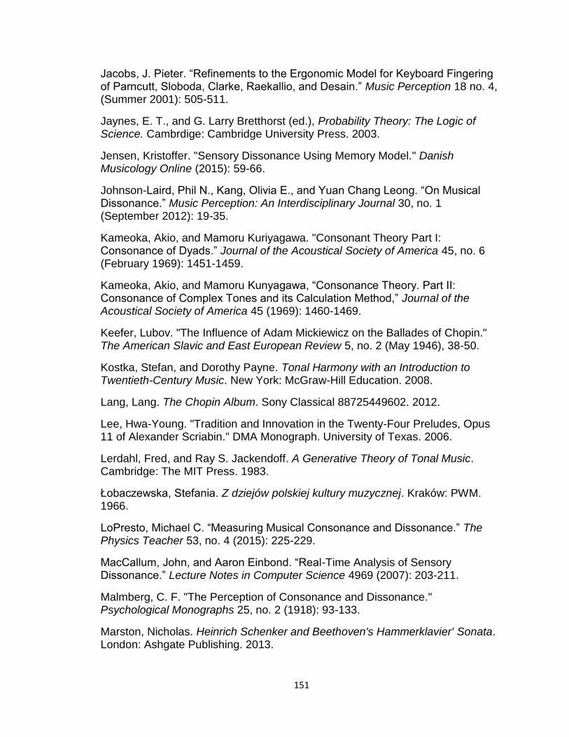
151

Jacobs, J. Pieter. “Refinements to the Ergonomic Model for Keyboard Fingering of Parncutt, Sloboda, Clarke, Raekallio, and Desain.” Music Perception 18 no. 4, (Summer 2001): 505-511.

Jaynes, E. T., and G. Larry Bretthorst (ed.), Probability Theory: The Logic of Science. Cambrdige: Cambridge University Press. 2003.

Jensen, Kristoffer. "Sensory Dissonance Using Memory Model." Danish Musicology Online (2015): 59-66.

Johnson-Laird, Phil N., Kang, Olivia E., and Yuan Chang Leong. “On Musical Dissonance.” Music Perception: An Interdisciplinary Journal 30, no. 1 (September 2012): 19-35.

Kameoka, Akio, and Mamoru Kuriyagawa. "Consonant Theory Part I: Consonance of Dyads.” Journal of the Acoustical Society of America 45, no. 6 (February 1969): 1451-1459.

Kameoka, Akio, and Mamoru Kunyagawa, “Consonance Theory. Part II: Consonance of Complex Tones and its Calculation Method,” Journal of the Acoustical Society of America 45 (1969): 1460-1469.

Keefer, Lubov. "The Influence of Adam Mickiewicz on the Ballades of Chopin." The American Slavic and East European Review 5, no. 2 (May 1946), 38-50.

Kostka, Stefan, and Dorothy Payne. Tonal Harmony with an Introduction to Twentieth-Century Music. New York: McGraw-Hill Education. 2008.

Lang, Lang. The Chopin Album. Sony Classical 88725449602. 2012.

Lee, Hwa-Young. "Tradition and Innovation in the Twenty-Four Preludes, Opus 11 of Alexander Scriabin." DMA Monograph. University of Texas. 2006.

Lerdahl, Fred, and Ray S. Jackendoff. A Generative Theory of Tonal Music. Cambridge: The MIT Press. 1983.

Łobaczewska, Stefania. Z dziejów polskiej kultury muzycznej. Kraków: PWM. 1966.

LoPresto, Michael C. “Measuring Musical Consonance and Dissonance.” The Physics Teacher 53, no. 4 (2015): 225-229.

MacCallum, John, and Aaron Einbond. “Real-Time Analysis of Sensory Dissonance.” Lecture Notes in Computer Science 4969 (2007): 203-211.

Malmberg, C. F. "The Perception of Consonance and Dissonance." Psychological Monographs 25, no. 2 (1918): 93-133.

Marston, Nicholas. Heinrich Schenker and Beethoven's Hammerklavier' Sonata. London: Ashgate Publishing. 2013.

152

Meyer, Leonard B. Explaining Music: Essays and Explorations. Berkeley, CA: University of California Press. 1973.

Mickey, Daniel Dewitt. “An Analysis of Texture in Selected Piano Études of Chopin and Scriabin.” Master's Thesis. Ohio State University. 1980.

Miskiewicz, Andrzej, and Andrzej Rakowski. "Loudness Level Versus Sound-Pressure Level: A Comparison of Musical Instruments." The Journal of the Acoustical Society of America 96, no. 6 (1994): 203-216.

Morris, Robert. “Mathematics and the Twelve-Tone System: Past, Present, and Future.” Perspectives of New Music 45, no. 2 (Summer 2007): 76-107.

Narmour, Eugene. “Implication – Realization: Continuous Bottom-Up Non-Closure Versus Top-Down Closural Structuration.” In Music in the Social and Behavioral Sciences: An Encyclopedia, edited by William Forde Thompson. Paris: Saga Publications. 2014.

Narmour, Eugene. The Analysis and Cognition of Melodic Complexity: The Implication-Realization Model. Chicago: The University of Chicago Press. 1992.

Nicomachus of Gerasa. Introduction to Arithmetic. Translated by Martin Luther D'Ooge. London: Johnson Reprint Corp. 1972.

Niecks, Frederick. Frederick Chopin, as a Man and Musician. London: Novello Inc. 1890.

Palmer, William A. Chopin: An Introduction to his Piano Works. New York, NY: Alfred Publishing. 1971.

Parks, Richard. “Voice Leading and Chromatic Harmony in the Music of Chopin.” Journal of Music Theory 20, no. 2 (Autumn 1976): 189-214.

Parncutt, Richard, John A. Sloboda, Eric F. Clarke, Matti Raekallio, and Peter Desain. “An Ergonomic Model of Keyboard Fingering for Melodic Fragments.” Music Perception 14 no. 4 (Summer 1997): 341-382.

Pen, Ronald Introduction to Music. New York: McGraw-Hill. 1992.

Pickens, Jeremy. “Harmonic Modeling for Polyphonic Music Retrieval.” Phd. Diss. University of Massachusetts. 2004.

Pollini, Maurizio. Chopin Études. Deutsche Grammophon 00289-477-8423. 1985.

Poniatowska, Irena. Fryderyk Chopin: A Poet of Sound.

Poniatowska, Irena. Fryderyk Chopin: The Man and his Music. Warsaw: Multico Oficyna Wydawnicza. 2010.

Poniatowska, Irena. Historia i interpretacja muzyki. Z badań nad muzykš od XVII do XVIII wieku. Warsaw: Musica Iagellonica. 1995.

153

Pulver, Jeffrey. "Walter Odington: The Consonance of the Third, and the Common Chord." The Musical Times 69, no. 1030 (December 1928): 1086-1088.

Reenan, Samuel, and Richard Bass. "Types and Applications of P3,0 Seventh-Chord Transformations in Late Nineteenth-Century Music." Music Theory Online 22, no. 2 (June 2016).

Richter, Sviatoslav. Richter Plays Chopin. Мелодия 10-01626. 2012.

Rimm, Robert. The Composer-Pianists: Hamelin and the Eight. Portland, OR: Amadeus Press. 2002.

Rink, John. The Practice of Performance: Studies in Musical Interpretation. Cambridge: Cambridge University Press. 1995.

Rochberg, George. A Dance of Polar Opposites: The Continuing Transformation of Our Musical Language. Rochester, NY: Rochester University Press. 2012.

Rosen, Charles. The Romantic Generation. Cambridge: Harvard University Press. 1998.

Rosenblum, Sandra P. "The Uses of Rubato in Music, Eighteenth to Twentieth Centuries." Performance Practice Review 7, no. 1 (Spring 1994): 33-53.

Samson, Jim. Chopin Studies, Volume 1. Cambridge: Cambridge University Press, 1988.

Samsons, Jim. The Cambridge Companion to Chopin. Cambridge: Cambridge University Press. 1992.

Schachter, Carl and Joseph N. Straus (ed.). Unfoldings: Essays in Schenkerian Theory and Analysis. Oxford: Oxford University Press. 1990.

Schenker, Heinrich. Der Freie Satz, Volume III. New York: Longman. 1935.

Schmitz, Robert. The Piano Works of Claude Debussy. New York: Dover. 1966.

Scruton, Roger. The Aesthetic Understanding. London: Methuen. 1983.

Shishkin, Dmitry. Chopin. Études, Polonaise in A-flat Major Op. 53, Scherzo in B-flat Minor Op. 31. Fryderyk Chopin Institute B01LWQ527E. 2016.

Schuijer, Michiel. Analyzing Atonal Music: Pitch-Class Set Theory and Its Contexts. Rochester, NY: University of Rochester Press, 2008.

Schumann, Robert. "Die Pianoforte-Etuden, ihren Zwecken nach geordnet," [Eng: The Pianoforte Études, Categorized According to their Purposes], Neue Zeitschrift für Musik 11 (February 6, 1836).

Scriabin, Alexander. The Complete Preludes & Études for Pianoforte Solo. New York: Dover Publications. 1973.

154

Smendzianka, Regina. How to Play Chopin? Part 3: Chopin's Études.

Spicer, Mark. “An Application of Grundgestalt Theory in the Late Chromatic Music of Chopin: A Study of His Last Three Polonaises.” PhD diss., University of North Texas. 1994.

Spicer, Mark J. “Root Versus Linear Analysis of Chromaticism: A Comparative Study of Selected Excerpts from the Oeuvres of Chopin.” College Music Symposium 36 (1996): 138-147.

Straus, Joseph N. Introduction to Post-Tonal Theory. Upper Saddle River, NJ: Pearson, 205.

Szklener, Artur. Chopin in Paris: The 1830s. Warsaw: Narodowy Instytut Fryderyka Chopina. 2006.

Szymanowska, Maria. Vingt Exercices et Préludes pour le Pianoforte. Warsaw: Première Livraison. 1819.

Taruskin, Richard. Music in the Nineteenth Century: The Oxford History of Western Music. Oxford: Oxford University Press. 2010.

Temperley, David. "The Tonal Properties of Pitch-Class Sets: Tonal Implication, Tonal Ambiguity, and Tonalness." Tonal Theory for the Digital Age: Computing in Musicology 15 (2007): 24-38.

Tenney, James. A History of “Consonance” and “Dissonance.” New York: Excelsior Music Publishing Company. 1988.

Terhardt, Ernst. "Pitch Consonance, and Harmony." The Journal of the Acoustical Society of America 55 no. 5 (May 1974): 1061-1069.

Tomaszewski, Mieczysław. Chopin: Człowiek, Dzieło, Rezonans. Poznań: Podsiedlik. 1998.

Verbalis, Jon. Natural Fingering: A Topographical Approach to Pianism. Oxford: Oxford University Press. 2012.

Virtala, Paula, and Mari Tervaniemi. "Neurocognition of Major-Minor and Consonance-Dissonance." Music Perception 34, no. 4 (April 2017): 387-404.

White, William Christopher, and Ian Quinn. “The Yale-Classical Archives Corpus.” Empirical Musicology Review 11, no. 1 (2016): 50-58.

Witten David. Nineteenth-Century Piano Music: Essays in Performance and Analysis. New York: Garland Publishing Inc. 1997.

Yip, Sheung Yung Joyce. "Tonal and Formal Aspects of Selected Mazurkas of Chopin: A Schenkerian View." PhD Diss., University of Michigan. 2010.

155

Zakrzewska, Dorota. "Alienation and Powerlessness: Adam Mickiewicz's ‘Ballady’ and Chopin's Ballades." Polish Music Journal 2, no. 1 (1999): 1-38.

Zavlunov, Daniil. "The 'tselostnyi analiz' (holistic analysis) of Zuckerman and Mazel." Music Theory Online 20, no. 3 (2014).

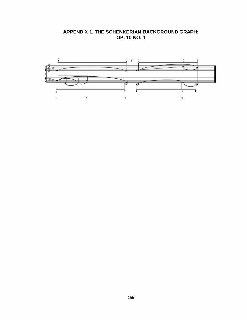
156

APPENDIX 1. THE SCHENKERIAN BACKGROUND GRAPH: OP. 10 NO. 1

157

APPENDIX 2. THE SCHENKERIAN FOREGROUND GRAPH: OP. 10 NO. 1

158

159

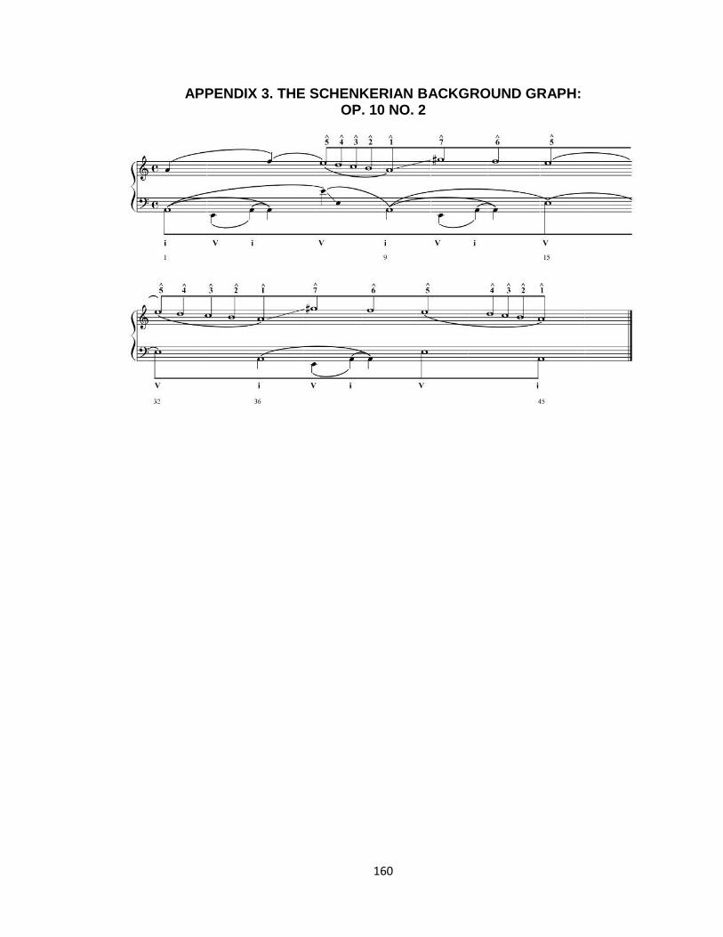
160


161


162

163

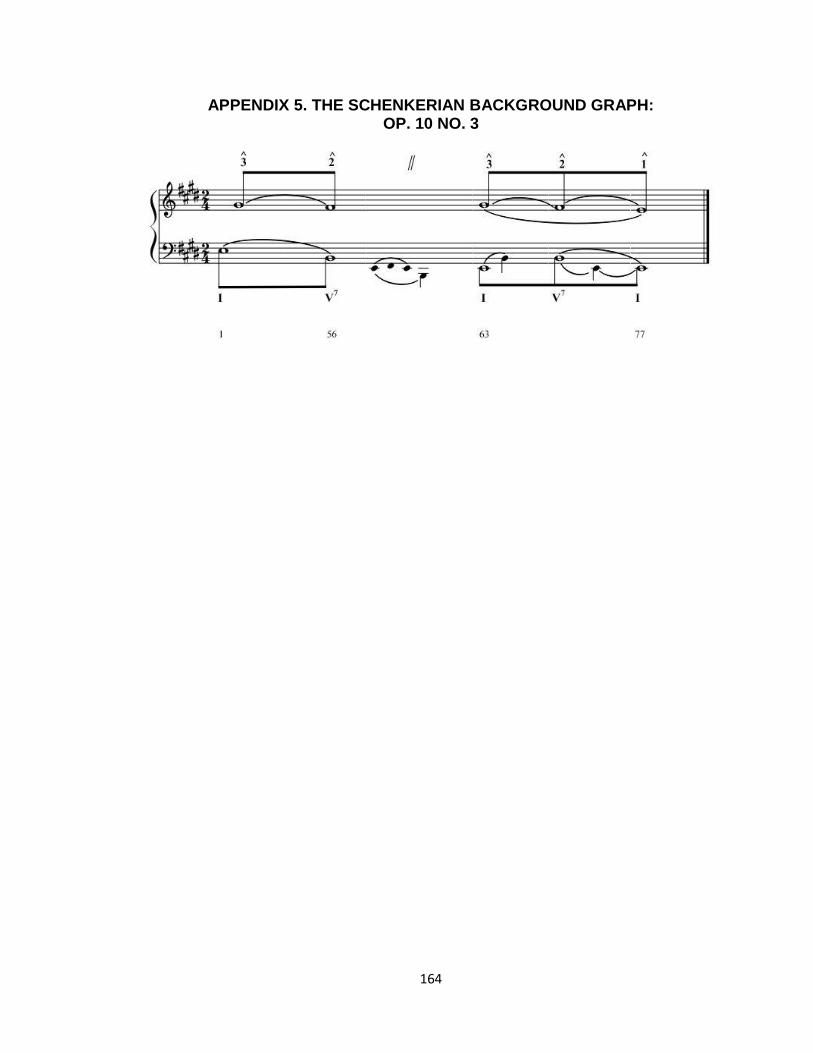
164


165


166

167

168


169


170

171

172

173

174

APPENDIX 9. THE SCRIPT TO COMPUTE IDR

=IF (n = "Cbb",0, IF(n = "Cb",1, IF(n = "C",3, IF(n = "C#",7, IF(n = "C##",15, IF(n = "Dbb",31, IF(n = "Db",63, IF(n = "D",127, IF(n ="D#",255, IF(n = "D##",511, IF(n = "Ebb",1023, IF(n = "Eb",2047, IF(n = "E",4095, IF(n = "E#",8191, IF(n = "E##",16383, IF(n = "Fbb",32767, IF(n="Fb",65535, IF(n = "F",131071, IF(n = "F#",262143, IF(n = "F##",524287, IF(n="Gbb",1048575, IF(n = "Gb",2097151, IF(n = "G",4194303, IF(n = "G#",8388607, IF(n="G##",16777215, IF(n = "Abb",33554431, IF(n = "Ab",67108863, IF(n = "A",134217727, IF(n="A#",268435455, IF(n = "A##",536870911, IF(n = "Bbb",1073741823, IF(n="Bb",2147483647, IF(n = "B",4294967295, IF(n = "B#",8589934591, IF(n="B##",17179869183, IF(n = "r","--"))))))))))))))))))))))))))))))))))))

175

VITA

Nikita Mamedov is a native of St. Petersburg, Russia and is currently in the

process of completing his PhD in Music Theory at Louisiana State University. He

received his Master's degree in Piano Performance & Pedagogy and his

Bachelor's degree in Piano and Music Theory & Composition from Rider

University.

Documents

The Interval Dissonance Rate in Chopin’s Études Op. 10