Embed Size (px)
Citation preview

The Introduction of a Knowledge-based Approach and Statistical Methods to Make GIS-Compatible Climate Map
Goshi Fujimoto
at MIG seminar on 16th, May
Daly, C. et al., 2002; Climate Research, vol. 22, 99-113.
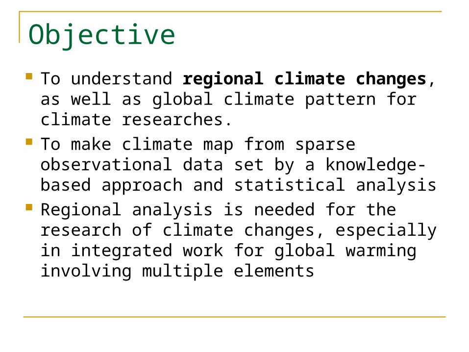
Objective To understand regional climate
changes, as well as global climate pattern for climate researches.
To make climate map from sparse observational data set by a knowledge-based approach and statistical analysis
Regional analysis is needed for the research of climate changes, especially in integrated work for global warming involving multiple elements

Introduction Knowledge-based approach
Based on topographic analyses The correlation of point climate data and topographic pos
ition, slope, exposure, elevation, and wind speed and direction
Statistical method To weight irregularly spaced point data to estimate
a regularly spaced prediction grid Inverse-distance weighting Kriging Splining

PRISM - Parameter-elevation Regressions on Independent Slopes Model
Fig. 1 The conceptual structure of a knowledge-based system for climate.

Regression function
A regression function between climate and elevation is the main predictive equation. A linear regression is adapted Y = β1X + β0 [ β1m ≤ β1 ≤ β1x ]
where Y is the predicted climate element, β1 and β0 are the regression slope and intercept. X is the elevation at the target grid cell. And β1m and β1x are the minimum and maximum regression slopes (Table 1).

Searching area from target grid cell The climate-elevation regression is developed from
pairs of elevation and climate observations.
Make a regression line : the range of β1, regression slope, must be between β1m and β1x.
is needed number of st, minimum number of total stations desired in regression : 10 or 15 or 30 stations

The knowledge base
The knowledge base is considered for weighting the various of correlations of climate stations and several elements.
Elevational influence on climate Terrain-induced climate transitions, ‘facets’ Coastal effects Two-layer atmosphere

Station weighting Upon entering the regression function, each station i
s assigned a weight that is based on several factors. The combined weight, W, is given as follows: W = [FdW(d)2 + FzW(z)2]1/2W(c)W(l)W(f)W(p)W(e)
where W(d), W(z), W(c), W(l), W(f), W(p), and W(e) are the distance, elevation, cluster, vertical layer, topographic facet, coastal proximity, and effective terrain weights, respectively. Fd and Fz are the distance and elevation weighting importance factors.

The distance weighting A station’s influence is assumed to decrease
as its distance from the target grid cell increases. The distance weight is given as:
where d is the horizontal distance and a is the
distance weighting exponent, is typically set to 2, which is equivalent to an inverse-distance-squared weighting function.

The elevation weighting A station’s influence is assumed to decrease as its verti
cal distance from the target gid cell increases. The elevation weight is given as:
where Δz is the elevation difference, b is the elevation weighting exponent, is typically set to 1, which is equivalent to a 1-dimensional inverse-distance weighting function. Δzm is the minimum elevation difference, and Δzx is the maximum one.

Topographic facets Delineation of topographic facets
The smoothed elevation for 6 levels is prepared by applying a Gaussian filter. The filtering wavelength is controlled by a maximum wavelength, λx.
Determination of each facets orientationby computing from elevation gradients between the 4 adjacent cells and assignedto an orientation on an 8 point compass.
Gaussian filter to the each levels
1
2
3
4
5
6

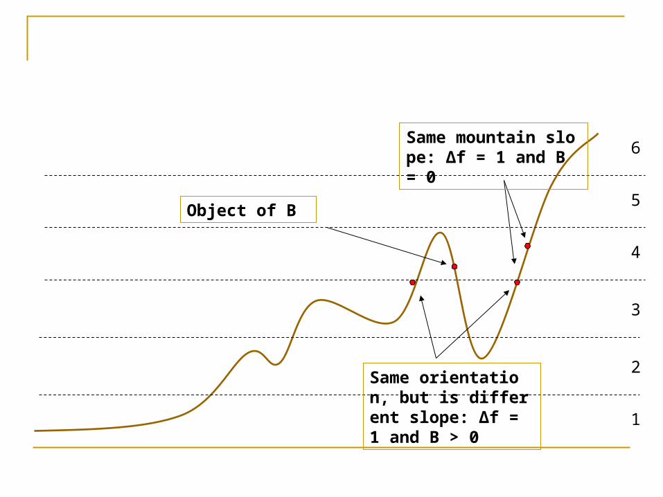
The facet weight The facet weight for a station is calculated as:
where Δf is the orientation difference (maximum possible difference is 4 compass points, or 180°), B is the number of intervening barrier cells with a different orientation with that of the target cell. c is the facet weighting exponent, which is typically set at 1.5 to 2.0, because of the rain shadows that can occur to the leeward of coastal mountains. In inland and flat regions, where rain shadows are less pronounced, a value of 1.5 or less will suffice.
1
2
3
4
5
6Same mountain slope: Δf = 1 and B = 0
Same orientation, but is different slope: Δf = 1 and B > 0
Object of B
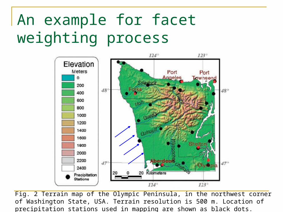
An example for facet weighting process
Fig. 2 Terrain map of the Olympic Peninsula, in the northwest corner of Washington State, USA. Terrain resolution is 500 m. Location of precipitation stations used in mapping are shown as black dots.

(b)
Fig. 3 Topographic facet grids overlain on shaded terrain grids for the Olympic Peninsula delineated at 2 wavelengths; (a) 4 km and (b) 60 km
Estimation of facet direction

Precipitation map for the Olympic Mountain
Fig. 4. Mean annual (1961–1990) precipitation with: (a) elevation regression functions and topographic weighting at each grid cell; (b) same as (a) except without topographic facet weighting; and (c) same as (b) except without terrain (all elevations set to zero). Mapping grid resolution is 4 km.
(b)
(c)
Evidence : on the windward, mean annual runoff is
3452 mm : in the Hoh River watershed
3442 mm : in the Queets River watershed
4042 mm : in the Quinault River watershed

Coastal proximity weight Coastal proximity grids have been developed that estima
te the proximity of each grid cell to major water bodies. Its weight for a station is calculated as:
where Δp is the absolute difference between the station and target cell, y is the coastal proximity weighting exponent, is typically set at 1.0, and px is the maximum proximity difference.

An example for coastal proximity
Fig. 5 Map of 1961–1990 mean August maximum temperature for the coast of central California (a) without and (b) with coastal proximity weighting. Open squares denote locations of coastal stations. Solid dots denote inland stations. Modeling grid resolution is 4 km.

The vertical layer weight
To simulate situations where non-monotonic relationships between climate and elevation are possible, climate stations are divided into 2 vertical layers.
The vertical layer weight is given as follows:
where Δl is the layer difference (1 for adjacent layer, 0 for same layer), Δz is the elevation difference, and y is the vertical layer weighting exponent. Δzm is the minimum elevation difference. A value of y is 0.5 to 1.0.

Estimation of potential wintertime inversion height
Fig. 6 Estimated wintertime inversion layer grid for the conterminous US. Shaded areas denote terrain estimated to be in the free atmosphere (layer 2) under winter inversion conditions, should they develop. Unshaded areas are expected to be within the boundary layer (layer 1). Grid resolution is 4 km.

Apply to my future work Adaptation to the case in Japan (Hokkaido?)
this algorithm Japan has much observation points than United
States of America in this case. Application to global warming conditions (by
several global warming scenarios) based on the case in Japan above
Adding to various of elements, correlations of climate and the vegetation, the population, and the economy, in this algorithm for integrated research for global warming.


![HANE GOSHI - Junomichi · is a hip technique [Koshi Waza] integrated into the Gokyo no Waza deve-lopped by Judo founder Master Jigoro Kano. Hane Goshi is the 5th hip](https://img.pdfslide.net/doc/110x75/5be5d92909d3f2ea1a8c2ea6/hane-goshi-junomichi-is-a-hip-technique-koshi-waza-integrated-into-the-gokyo.jpg)