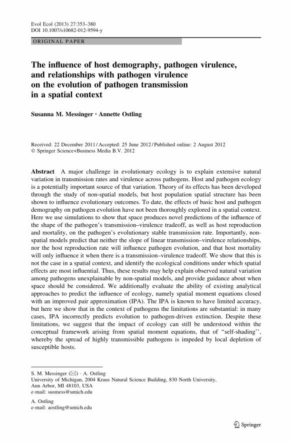
ORI GIN AL PA PER

The influence of host demography, pathogen virulence,and relationships with pathogen virulenceon the evolution of pathogen transmissionin a spatial context

Susanna M. Messinger • Annette Ostling

Received: 22 December 2011 / Accepted: 25 June 2012 / Published online: 2 August 2012� Springer Science+Business Media B.V. 2012

Abstract A major challenge in evolutionary ecology is to explain extensive natural

variation in transmission rates and virulence across pathogens. Host and pathogen ecology

is a potentially important source of that variation. Theory of its effects has been developed

through the study of non-spatial models, but host population spatial structure has been

shown to influence evolutionary outcomes. To date, the effects of basic host and pathogen

demography on pathogen evolution have not been thoroughly explored in a spatial context.

Here we use simulations to show that space produces novel predictions of the influence of

the shape of the pathogen’s transmission–virulence tradeoff, as well as host reproduction

and mortality, on the pathogen’s evolutionary stable transmission rate. Importantly, non-

spatial models predict that neither the slope of linear transmission–virulence relationships,

nor the host reproduction rate will influence pathogen evolution, and that host mortality

will only influence it when there is a transmission–virulence tradeoff. We show that this is

not the case in a spatial context, and identify the ecological conditions under which spatial

effects are most influential. Thus, these results may help explain observed natural variation

among pathogens unexplainable by non-spatial models, and provide guidance about when

space should be considered. We additionally evaluate the ability of existing analytical

approaches to predict the influence of ecology, namely spatial moment equations closed

with an improved pair approximation (IPA). The IPA is known to have limited accuracy,

but here we show that in the context of pathogens the limitations are substantial: in many

cases, IPA incorrectly predicts evolution to pathogen-driven extinction. Despite these

limitations, we suggest that the impact of ecology can still be understood within the

conceptual framework arising from spatial moment equations, that of ‘‘self-shading’’,

whereby the spread of highly transmissible pathogens is impeded by local depletion of

susceptible hosts.

S. M. Messinger (&) � A. OstlingUniversity of Michigan, 2004 Kraus Natural Science Building, 830 North University,Ann Arbor, MI 48103, USAe-mail: susmess@umich.edu

A. Ostlinge-mail: aostling@umich.edu

123

Evol Ecol (2013) 27:353–380DOI 10.1007/s10682-012-9594-y

Keywords Spatial structure � Pathogen evolution � Pair approximation � Host ecology �Transmission–virulence tradeoff

Introduction

A significant challenge in disease ecology is to explain the tremendous natural variation in

pathogen transmission and virulence across pathogen species. A potentially important

source of variation is host and pathogen ecology. For example, the tuberculosis pathogen

(Mycobacterium tuberculosis) is highly virulent (causes high host mortality) while pneu-

monia (Mycoplasma pneumoniae) is much less virulent (Walther and Ewald 2004). One

possible explanation is that the bacteria causing tuberculosis can survive upwards of

250 days in the environment while the bacteria causing pneumonia can survive less than

2 days in the environment (Bonhoeffer et al. 1996; Walther and Ewald 2004). Thus, the

negative impact of virulence on pathogen fitness, mediated by host mortality, is less for

tuberculosis than pneumonia. The evolutionary importance of environmental pathogen

transmission has been more generally addressed in the literature (e.g., Roche et al. 2011;

Gandon 1998; Day 2002). Other highly cited ecological explanations for observed varia-

tion in pathogen transmission and virulence include the presence and shape of a trans-

mission–virulence tradeoff (Levin and Pimentel 1981; Anderson and May 1982; May and

Anderson 1982), the timing of transmission (Cooper et al. 2002; Day 2003; Osnas and

Dobson 2010), the mode of transmission (Ewald 1987, 1998; White et al. 2002), and the

occurrence of co-infection or super-infection (Levin and Pimentel 1981; Bull 1994; Levin

and Bull 1994; van Baalen and Saebelis 1995; Frank 1996; Mosquera and Adler 1998;

Nowak and Sigmund 2002; Alizon and Lion 2011).

Our current understanding of the evolutionary influence of host and pathogen ecology is

largely based on analysis of mathematical models or inference from observational studies

(e.g., Ewald 1993). Empirical studies are limited by the difficulty of isolating the evolu-

tionary influence of one particular ecological factor on pathogen variation. As methods in

the study of evolutionary ecology become more sophisticated, observational and theoretical

predictions are increasingly being tested (e.g., de Roode et al. 2008; Eshelman et al. 2010).

Yet the mathematical theory being tested has been developed primarily from analysis of

non-spatial pathogen-host models. Recent theoretical work suggests that spatial context can

strongly influence the evolution of interacting species (Johnson and Seinen 2002; Le Gal-

liard et al. 2003; Hansen et al. 2007; Prado and Kerr 2008), including pathogens (Boots and

Sasaki 1999; Haraguchi and Sasaki 2000; Rauch et al. 2002; Kerr et al. 2006; Kamo et al.

2007; Lion and van Baalen 2008; Messinger and Ostling 2009; Boerlijst and van Balle-

gooijen 2010). This is especially relevant for pathogens since host populations are often

naturally structured by intrinsic limitations on movement, ranging from immobility (e.g.,

plants) to restricted home ranges (e.g., many mammal species).

While some theoretical work has addressed the evolutionary impact of host and path-

ogen ecology in a spatial context (Claessen and de Roos 1995; Boots et al. 2004; Kamo and

Boots 2004; Caraco et al. 2006; Kamo et al. 2007), the impact of basic host demography on

the evolution of pathogen transmission has not been thoroughly explored. Furthermore, we

have only pieces of the whole picture regarding the impact of the shape of the relationship

between the pathogen’s transmission rate and virulence in a spatial context (see: Boots and

Sasaki 1999; Haraguchi and Sasaki 2000; Kamo et al. 2007). In particular, lacking is a

systematic exploration of the pathogen’s ES transmission rate across both host

354 Evol Ecol (2013) 27:353–380

123

demography, relationships between the pathogen’s transmission and virulence, and path-

ogen virulence when there is no transmission–virulence relationship. Given that these

aspects of ecology are fundamental to hosts and their pathogens, elucidating their effects in

a spatial context may improve our understanding of trait variation across of a broad range

of pathogen species.

Here we evaluate via simulations the predicted effect of the shape of the pathogen’s

transmission-virulence relationship on the pathogen’s evolutionary stable (ES) transmis-

sion rate. In addition, we evaluate the predicted effect of the host reproduction rate, host

natural death rate, and pathogen virulence on the pathogen’s ES transmission rate for no

transmission–virulence relationship and across a range of linear and concave-down

transmission–virulence relationships. We find that the ecological context set by these traits

is an important determinant of the pathogen’s ES transmission rate even when the non-

spatial model predicts they are not. Particularly important is host reproduction: high host

reproduction leads to a higher ES transmission rate. In most cases, host death increases the

ES transmission rate, but at high host reproduction rates the ES transmission rate can

actually decline. Though in some cases the spatial and non-spatial models predict the same

qualitative trends with ecology, the quantitative difference varies. In some ecological

contexts the quantitative differences are substantial, suggesting that despite overarching

qualitative consistency in the theoretical predictions of spatial and non-spatial models, the

potential evolutionary effects of spatial structure should not be ignored.

Given the potential of these results to inform our understanding of pathogen evolution,

as well as the computational difficulties associated with deriving them for all possible

ecological contexts, we additionally evaluate the ability of existing analytical approaches

to predict them. Researchers have debated about the best way to quantify pathogen fitness

in space and thus predict the evolutionary influence of the ecological context (Slobodkin

1974; van Baalen and Rand 1998; Boots and Sasaki 1999, e.g., compare interpretations of

pathogen fitness in: Johnson and Boerlijst 2002; Kerr and Godfrey-Smith 2002; and Rauch

et al. 2002, also see: Goodnight et al. 2008). A recent key approach has been to quantify

pathogen fitness through the use of spatial moment equations: coupled equations that

describe the mean density and spatial arrangement of hosts in a population. These equa-

tions enable one to deconstruct fitness into its spatial and non-spatial components and thus

more clearly understand how spatial structure will influence the evolution of a particular

trait as well as the effect of different ecological contexts. In particular, these equations

have highlighted the evolutionary role of ‘‘self-shading’’, when the growth of cheaters or

over-exploiters is hindered by the depletion of local resources, and host demography

(Boots and Sasaki 1999; Lion and Boots 2010).

Although conceptually insightful, the tractability of the fitness concept based on spatial

moment equations depends on the use of a moment closure method. A frequently used

method is a pair approximation (PA) (see Boots and Sasaki 2000; Caraco et al. 2006; Kamo

and Boots 2006; Kamo et al. 2007) that eliminates the infinite array of moments above

pairs of individuals (Matsuda et al. 1992; Harada and Iwasa 1994; Sato et al. 1994).

Though it is common knowledge that pair approximations are not always accurate, it is not

clear to what extent for host-pathogen interactions. A few recent studies have questioned

the accuracy of the PA in predicting the pathogen’s ES transmission rate when the path-

ogen is not subject to a transmission–virulence relationship (de Aguiar et al. 2004; Boots

et al. 2006; Lion and Boots 2010), demanding a more comprehensive evaluation.

Here we evaluate the ES transmission rate predicted using the improved pair approx-

imation (IPA), which has commonly been used in studies of spatial pathogen-host

dynamics, in comparison to that predicted by spatial simulations. We find that predictions

Evol Ecol (2013) 27:353–380 355

123

based on IPA can be qualitatively incorrect, and fail to the largest degree when the effects

of spatial structure are most significant. This demonstrates the previously unknown extent

of the limitations of IPA in predicting the effect of spatial structure on pathogen evolution

and advocates examination of the accuracy of other moment closure methods (e.g., Filipe

and Maule 2003; Bauch 2005; Peyrard et al. 2008). However, despite the limitations of the

IPA, we find that the relationships with host and pathogen demography uncovered through

simulation can still be conceptually understood within the framework of ‘‘self-shading’’.

We suggest that future work should explore new constructs for quantifying the effects of

‘‘self-shading’’.

Non-spatial model and predictions

A standard non-spatial model of susceptible-infected host-pathogen dynamics is given by

the following equations:dS

dt¼ ðr � dÞ � S� b � S � I ð1Þ

dI

dt¼ b � S � I � ðd þ aÞ � I ð2Þ

In this model, S is the number of susceptible hosts, I is the number of infected hosts, d is

the host natural death rate, r is the host reproduction rate, b is the infection rate per infected

individual, and a is the pathogen virulence (the death rate of the host due to infection). The

product of b and I is the infection rate. Thus, b�S�I is the number of susceptible hosts that

become infected per time assuming complete mixing of the host population. This model

assumes that infected hosts do not recover from infection but are removed from the

population due to natural death or disease-induced death. A number of real pathogen-host

systems conform to this assumption, ranging from very virulent pathogens like lethal

yellowing disease to nearly avirulent pathogens like Herpes. The model also assumes that

hosts cannot be co-infected. As mentioned, co-infection has been shown to play an

important role in pathogen evolution (Levin and Pimentel 1981; Bull 1994; Levin and Bull

1994; Frank 1996; Mosquera and Adler 1998; Nowak and Sigmund 2002). Here, however,

our goal is to more carefully explore the role of a limited set of basic host and pathogen

ecology related only to demography. As such, we choose to build from a simple model that

does not include evolutionary complexities like co-infection.

From the above model, a pathogen’s per-capita growth rate is

1

I� dI

dt¼ b � S� d þ a

b

� �ð3Þ

where S is the number of susceptible hosts experienced by the pathogen. Given some

number of susceptible hosts, the per-capita growth rate decreases with infected host

mortality and increases with transmission. The quantity (d ? a)/b has special significance:

it is the expected equilibrium number of susceptible hosts in a monomorphic population,

S*. Thus, the pathogen’s per-capita growth rate can be re-written as

1

I� dI

dt¼ b � S� S�ð Þ ð4Þ

and the pathogen population is predicted to grow if the actual number of susceptible hosts

it experiences is greater than the number expected at equilibrium. S* is the inverse of the

356 Evol Ecol (2013) 27:353–380

123

pathogen’s epidemiological R0 (the number of secondary infections caused per infected

individual over its infectious period in a completely susceptible population; Eq. 5).

R0 ¼b

d þ að5Þ

To understand the evolutionary dynamics predicted by this model, we consider the per-

capita growth rate of a pathogen from rarity in a dimorphic population, where the host

population is already at equilibrium with a resident pathogen strain. In this scenario, both

pathogens experience the same actual number of susceptible hosts (S from Eq. 4), which is

the number of susceptible hosts at equilibrium with the resident pathogen. Thus,

1

Iinvader� dIinvader

dt¼ Binvader � S�resident � S�invader

� �ð6Þ

If the invader’s expected equilibrium number of susceptible hosts in a monomorphic

population (Sinvader* ) is less than the actual number it experiences (Sresident

* , which is also the

expected equilibrium number of susceptible hosts in a monomorphic population with just

the resident), the invasion will succeed. In terms of R0, the pathogen with the bigger R0 can

invade. Therefore, this model predicts that selection will maximize R0. Note that the

pathogen’s per-capita growth rate is no different if the host is assumed to have logistic

rather than exponential growth—the predictions arising from the following invasion

analysis are not dependent on any assumptions about the host’s growth. This is important

since our spatial model effectively regulates the host’s growth.

We can understand the non-spatial evolutionary influence of host and pathogen ecology

by finding the transmission rate that maximizes R0 (Eq. 5). Assuming there can be a

relationship between the pathogen’s transmission rate and virulence (a = C�bz), the ES

transmission rate that maximizes R0 is

b ¼ffiffiffiffiffiffiffiffiffiffiffiffiffiffiffiffiffiffiffiffiffi

d

C � ðz� 1Þz

sð7Þ

When there is no transmission–virulence relationship (C = 0) or if the relationship is

linear (z = 1), the ES transmission rate is undefined: R0 is maximized by an infinite

transmission rate (and virulence, in the case of a linear transmission–virulence relation-

ship). In practice, the model predicts evolution to pathogen-driven host extinction. Only if

there is a transmission–virulence tradeoff (z [ 1) does the non-spatial model predict an

intermediate ES transmission rate. It follows that when there is no transmission–virulence

relationship or a linear transmission–virulence relationship, host and pathogen ecology are

not predicted to play a role in pathogen evolution. When there is a transmission–virulence

tradeoff, the ES transmission rate is predicted to increase with the constant of propor-

tionality (C) and the tradeoff exponent (z). The host reproduction rate is not predicted to

influence pathogen evolution when there is a transmission-virulence tradeoff (the param-

eter r does not even appear in Eq. 7), and the ES transmission rate is predicted to increase

with the host natural death rate (d).

Spatial model and predictions

Assuming the same basic susceptible-infected pathogen-host dynamics (no immunity or

co-infection), we consider a relatively simple stochastic spatial model where the host

Evol Ecol (2013) 27:353–380 357

123

population resides on a regular two-dimensional lattice (150 9 150). Lattice sites can be

occupied or empty, hosts are fixed in space, and host reproduction and pathogen trans-

mission only occur between directly adjacent lattice sites. The realized rate of host

reproduction is determined by the product of r and the number of empty sites among the

host’s four nearest-neighboring sites. Similarly, the realized rate of transmission is

determined by the product of b and the number of susceptible hosts among the infected

hosts four nearest-neighboring sites. Otherwise, the dynamics are as described for the non-

spatial model. Though simple, this type of spatial structure captures the key elements of

spatially-explicit host-pathogen dynamics and has already been demonstrated to have

significant evolutionary effects (Messinger and Ostling 2009). Hence it provides a good

starting point for understanding spatial effects on pathogen evolution. Furthermore, this

type of spatial structure is potentially representative of several natural host populations,

including plants, sedentary plant parasites like aphids and other scale insects, sessile

marine animals like barnacles, or animals with limited movement like anemones, starfish,

and some terrestrial invertebrates.

Note that in the spatial model, the realized host reproduction rate and pathogen trans-

mission rate differ from the rates quantified by the parameters r and b. The actual

parameter value reflects the rate if space were not limiting—in other words, if empty sites

for reproduction and susceptible hosts for infection were unlimited. For example, in the

absence of the pathogen, a reproduction rate of 25 per host generation yields a realized rate

of 3.67 per host generation. This is within the range of measured values of rmax for many

organisms. Despite the large discrepancy between the actual parameter value and the

resulting realized value, the two are always positively related. Thus, the trends in the ES

pathogen transmission rate with the actual value reflect the trends with realized value.

To find the ES transmission rate for the spatial model we simulate the dynamics as a

Poisson process using the Gillespie algorithm (Gillespie 1977). The algorithm computes

the time interval between sequentially occurring events, which is exponentially distributed

for a Poisson process. When an event occurs, the probability of a particular event (host

birth, host death, and pathogen transmission) is equal to the rate at which that event should

occur, divided by the total rate at which events occur. Each time a susceptible host is

infected, there is some chance that the infecting strain will mutate and acquire a different

transmission rate, slightly different than the parent strain. Starting from a low initial

transmission rate, the average transmission rate of the pathogen population changes over

time. When the average transmission rate is no longer changing over time, we run the

simulation for an additional 2,000 time steps and take the average over the last 2,000 time

steps as the ES transmission rate. Although this method has been used elsewhere (e.g., Best

et al. 2011), it is different than the method used in other papers (e.g., Kamo et al. 2007,

where the ES transmission rate is determined through the outcome of comprehensive pair-

wise invasions). We compared three different methods of inferring the ES transmission rate

and found no difference between them (Appendix 1).

We compare the influence of the shape of the transmission virulence relationship, the

host reproduction rate, the host death rate, and the pathogen virulence predicted by the

spatial model with the influence predicted by the non-spatial model. We make comparisons

for the following cases: no transmission virulence relationship, three types of linear

relationships (a = b/3, a = b/6, and a = b/10), and four types of tradeoffs (a = b1.1/10,

a = b1.3/10, a = b1.5/10, a = b1.7/10). For each relationship, including none, we examine

a range of host reproduction rates and natural host death rates. For the case of no trans-

mission–virulence relationship we also examine a range of pathogen virulence. For all

cases we also show the extinction threshold transmission rate (above which the endemic

358 Evol Ecol (2013) 27:353–380

123

equilibrium is unstable and the pathogen causes host extinction) and invasion threshold

transmission rate (below which the endemic equilibrium is unstable and the pathogen

cannot invade the host population) predicted from IPA. The thresholds predicted by

ordinary and improved PAs have been shown to be qualitatively accurate for the type of

dynamics and spatial structure examined here (Boots and Sasaki 2000; Haraguchi and

Sasaki 2000; Ohtsuka et al. 2006; Webb et al. 2007a, b).

Shape of the transmission–virulence relationship

Assuming a linear transmission–virulence relationship we corroborate over a much broader

parameter space the previous finding (e.g., Kamo et al. 2007) that the spatial model

predicts an intermediate ES transmission rate and endemism. We further find that the ES

transmission rate declines with increasing values of the constant of proportionality (C in

the equation a = C�bz when z = 1) for both low and high host reproduction rates (Fig. 1a).

In other words, steeper linear transmission–virulence relationships lead to lower ES

transmission rates. This is perhaps intuitive based on the non-spatial prediction that steeper

transmission–virulence tradeoffs lead to a lower ES transmission rate, but demonstrates

that spatial structure can induce evolutionary effects where non-spatial models predict

none.

Similar to the spatial model, assuming a transmission-virulence tradeoff, the spatial

model predicts a decline in the ES transmission rate with the tradeoff exponent (z in the

equation a = C�bz when C = 0.1; Fig. 1b). However, across all tradeoff exponents the

60

0

120

Tradeoff Exponent, z

1 1.1 1.3 1.91.5 1.7

spatial, r=100

non-spatial

spatial, r=30

(a)

(b)

∞

150

0

Tradeoff Proportionality Constant, C

0 0.1 0.2 0.3

75

Fig. 1 ES transmission ratesacross transmission–virulencerelationships. The EStransmission rates (ES b)obtained from simulation (datapoints) and predictions from thenon-spatial model (thick lines)are shown for differenttransmission–virulencerelationships and for two hostreproduction rates (r = 30,squares and dashed line;r = 100, triangles and solidline). a Linear transmission–virulence relationships, shapecontrolled by constant ofproportionality C in a = C�bz

when z = 1, b concave-downtransmission–virulence tradeoffs,shape controlled by tradeoffexponent z in a = C�bz whenC = 0.1

Evol Ecol (2013) 27:353–380 359

123

spatial ES transmission rate is lower than the non-spatial expectation—a trend that has

been hinted at (Messinger and Ostling 2009) but not fully demonstrated.

Host reproduction rate

In contrast to the non-spatial model, for all transmission-virulence relationships including

none, the spatial model predicts an intermediate ES transmission rate that varies with the

100

50

0

100

50

0

7

6.5

6

5.5

(a)

(b)

(c)

500 25

0 10050

0 10050

Host Reproduction Rate

spatial

non-spatial

∞

∞

Fig. 2 Effect of hostreproduction rate on EStransmission rate. Threeexamples of the ES transmissionrates (ES b) obtained fromsimulation (data points withdashed spline fit) and predictionsfrom the non-spatial model (thicklines) across host reproductionrates (r). The shaded areas areregions where the IPA predictsextinction of the host, pathogen,or both. In the region to the left,the host will go extinct due to aninsufficient reproduction rate. Inthe upper region the pathogendrives the host population anditself to extinction. In the lowerregion the pathogen cannotinvade the host population due toan insufficient transmission rate.In all cases, the non-spatialmodel predicts no trend with hostreproduction rate. a notransmission–virulencerelationship (a = 1), b lineartransmission–virulencerelationship (a = b/6), andc concave-down transmission–virulence tradeoff (a = 0.1�b1.5)

360 Evol Ecol (2013) 27:353–380

123

host reproduction rate (Fig. 2). In particular, assuming no transmission-virulence rela-

tionship, the ES transmission rate initially decreases and then increases with host repro-

duction rate for low host death rates (d = 1, d = 2) and pathogen virulence (a = 0,

a = 1). For higher host death rates (d = 3, d = 4) and pathogen virulence (a = 2, a = 3),

the ES transmission rate increases with host reproduction (d = 1 and a = 1 shown in

Figs. 2a, 9). Assuming a transmission–virulence relationship, either linear or a tradeoff, the

ES transmission rate increases with the host reproduction rate (Figs. 2b, c, 10, 11). Across

all host reproduction rates, the spatial ES transmission rate is always lower than the non-

spatial expectation assuming a transmission–virulence tradeoff.

Host mortality

In contrast to the non-spatial model, assuming no transmission–virulence relationship or a

linear relationship the spatial model predicts an increase in the ES transmission rate with

host death rate (Figs. 3a, b, 12, 13). Assuming no transmission virulence relationship, the

spatial model predicts a similar increase with pathogen virulence (Figs. 4, 12). Further, the

effect of host death rate and virulence diminishes as host reproduction rate increases,

actually reversing at high host reproduction rates such that an increase in host death or

virulence decreases the ES transmission rate. In addition, the death rate has a larger effect

than the virulence on the spatial ES transmission rate. Finally, the host death rate and

virulence most significantly influence evolution assuming no transmission–virulence

relationship when host reproduction is low.

Similar to the non-spatial expectation, assuming a transmission–virulence tradeoff the

non-spatial model predicts an increase in the ES transmission rate with host death rate

across all host reproduction rates (Figs. 3c, 13). However, the non-spatial model consis-

tently predicts a larger increase than the spatial model. In other words, the spatial model

predicts a weaker evolutionary effect of the host death rate.

Pair approximation

One way to capture the effects of the type of spatial structure described above is via spatial

moment equations that describe the time derivative of paired states on the lattice

(Appendix 2). Summing the appropriate state pair derivatives yields the time derivative for

infected hosts. From this analysis, a pathogen strain’s per-capita growth rate is

1

I� dI

dt¼ b

n� QðSjIÞ � d þ a

b

� �¼ b

n� ½QðSjIÞ � Q�ðSjIÞ� ð8Þ

In this equation, n is the number of lattice sites in the neighborhood of each host (here

n = 4), Q(S|I) is the actual average number of susceptible hosts in the neighborhood of an

infected host, Q*(S|I) is the expected average number at equilibrium in a monomorphic

population (which, like S* in the non-spatial model, is the inverse of the pathogen’s

epidemiological R0), and all other parameters are as defined for the non-spatial model.

Similar to the non-spatial model, the pathogen population is predicted to grow if the actual

number of susceptible hosts surrounding an infected host is bigger than the number

expected at equilibrium.

As with the non-spatial model, to understand the evolutionary dynamics predicted by

the spatial moment equations, we consider the growth rate of a pathogen from rarity in a

Evol Ecol (2013) 27:353–380 361

123

dimorphic population, where the host population is already at equilibrium with a resident

pathogen strain. If we make the assumption that the resident and invading pathogen

experience the same actual average number of susceptible hosts at the time of invasion

(Q(S|I) from Eq. 8) and that it is equal to the resident’s expected equilibrium value, the

invading pathogen’s per-capita growth rate is

0

1

3.5

Fact

or o

f In

crea

se

3

1

0

Host Reproduction Rate

d=2-3d=1-2

d=3-4

non-spatial

0

1

2

8 9 10 20 30 40 20 40 60 80 100 20 40 60 80 100

(a) (c)

Host Reproduction RateHost Reproduction Rate

(b)

Fig. 3 Effect of host natural death rate on ES transmission rate. Three examples of the factor of increase inthe ES transmission rates (ES b) with a unit increase in the host natural death rate (e.g., from d = 1 tod = 2) obtained from simulation (bars) and predictions from the non-spatial model (thick lines) across hostreproduction rates (r). A factor of increase of 1 represents no change in the ES b with death rate or virulence,a value greater than 1 is an increase, and a value less than 1 is a decrease. For no transmission–virulencerelationship and a linear relationship the non-spatial model predicts no change with host natural death rate(factor of increase = 1). a no transmission–virulence relationship (a = 1), b linear transmission–virulencerelationship (a = b/6), and c concave-down transmission–virulence tradeoff (a = 0.1�b1.1)

Host Reproduction Rate

2

1

0

Fact

or o

f In

crea

se

α=1-2α=0-1

α=3-4α=2-3

α=4-5

8 9 10 20 30 407654

Fig. 4 Effect of virulence on ES transmission rate for no transmission–virulence relationship. An exampleof the factor of increase in the ES transmission rate (ES b) with a unit increase in the virulence fromsimulations (bars) along with predictions from the non-spatial model (thick lines) is shown for a range ofhost reproduction rates. A value of 1 represents no change in the ES b with death rate or virulence, a valuegreater than 1 is an increase, and a value less than 1 is a decrease. The non-spatial model predicts no changewith pathogen virulence (factor of increase = 1). Other parameters: d = 1

362 Evol Ecol (2013) 27:353–380

123

1

Iinvader� dIinvader

dt¼ binvader

n� ½Q�ðSjIresidentÞ � Q�ðSjIinvaderÞ� ð9Þ

This leads to an invasion criterion similar to the non-spatial model: if the invader’s

expected equilibrium average number of susceptible hosts around an infected host in a

monomorphic population (Q*(S|Iinvader)) is less than the actual number it experiences

(Q*(S|Iresident)), which is also the expected equilibrium average number in a monomorphic

population with the resident), the invasion will succeed. However, in a spatial context the

resident and invading pathogen will not experience the same Q(S|I)—a rare invading

pathogen can have an immediate and large impact on the number of susceptible hosts in its

local neighborhood. Therefore, shortly after invasion, the resident pathogen will experi-

ence Q*(S|Iresident) susceptible hosts but the invading pathogen will experience a quasi-

equilibrium number, Q0(S|Iinvader). At quasi-equilibrium the invading strain is still rare but

has come to equilibrium with its local neighborhood (Matsuda et al. 1992). This yields

instead

1

Iinvader� dIinvader

dt¼ binvader

n� ½Q0ðSjIinvaderÞ � Q�ðSjIinvaderÞ� ð10Þ

By this equation, the invasion will succeed if Q0(S|Iinvader) is greater than Q*(S|Iinvader).

Note that even though this representation of the invasion fitness does not explicitly include

the resident strain, Q0(S|Iinvader) depends on how the resident pathogen has already shaped

the host population. For example, if there are very few susceptible hosts in the population

to begin with, the invader is unlikely to realize a high Q0(S|Iinvader). In addition, note that

Boots and Sasaki (1999) take this one step further to frame the invasion fitness as a balance

between the difference in 1/R0 of the resident and invader (well-mixed effects) and the

difference in Q(S|I) of the resident at equilibrium and invader at quasi-equilibrium (spatial

effects). This alternative representation implies that the resident pathogen must be

accounted for in ways beyond it’s effect on Q0(S|Iinvader), however, when interactions are

completely local, 1/R0 = Q*(S|I) for the resident and thus cancel out of the equation.

Equation 10 provides a conceptual framework for explaining the effect of spatial

structure on pathogen evolution. Because a highly transmissible pathogen quickly infects

neighboring susceptible hosts, it will tend to have a lower Q0(S|Iinvader), thus diminishing

its overall ability to invade the population. In effect, highly transmissible pathogens ‘‘self-

shade’’ themselves. The risk of ‘‘self-shading’’ will vary depending on the invasion con-

text. For example, if there are many susceptible hosts available upon invasion, the risk is

lower than if there are few. An alternative framework for explaining the effect of spatial

structure on pathogen evolution has more recently been proposed by Lion and Boots

(2010). They derive the selection gradient for the pathogen’s transmission rate. In this

framework, the risk of ‘‘self-shading’’ also depends on the invasion context: in addition to

the density of susceptible hosts around an infected host, it depends on the density of empty

sites around an infected host and the relatedness of neighboring pathogens.

Although conceptually insightful, Eq. 10 and the selection gradient formulated by Lion

and Boots (2010) are not closed: the average pair densities depend on higher order spatial

correlations. For example, the number of susceptible hosts next to infected hosts (Q(S|I))depends on higher order spatial moments (e.g., Q(S|IS)). The dependencies continue

upward in scale to the size of the entire lattice. Thus, in order to quantify pathogen fitness

or the selection gradient, one must use a moment closure method. A simple moment

closure method often used is the improved PA (IPA) (Sato et al. 1994). PAs take advantage

of the fact that the number of state triples on a lattice can be written in terms of the two

Evol Ecol (2013) 27:353–380 363

123

state pairs that it is composed of. If one makes certain assumptions about the distribution of

state triples across the lattice (see: Morris 1997), the relationship between state triples and

pairs simplifies so that correlations above pairs can be ignored. The IPA is a special PA

that accounts for the aggregation of susceptible hosts in space due to local reproduction

(Appendix 3).

Here we infer the ES transmission rate predicted by an IPA of the spatial moment

equations using Eq. 10. For each transmission-virulence relationship, including none, and

parameter set we numerically solve for the quasi-equilibrium Q(S|I) (method described in:

Kamo et al. 2007; see Appendix 4) and use it to calculate the invasion fitness for pairs of

resident and invading pathogens. The transmission rate of the pathogen that cannot be

invaded by any other pathogen strain is taken as the ES transmission rate. To find the

predicted extinction threshold transmission rate and the invasion threshold transmission

rate, we perform a stability analysis of the endemic equilibrium (methods described in:

Sato et al. 1994).

Somewhat surprisingly, we find that like the non-spatial model, assuming no trans-

mission–virulence relationship the IPA predicts evolution to an infinite transmission rate

across all host reproduction rates, host death rates, and pathogen virulence. Assuming a

linear transmission–virulence relationship, the IPA demonstrates inconsistent qualitative

accuracy in predicting the trends between the ES transmission rate and the shape of the

transmission–virulence relationship, host reproduction rate, and host death rate. In par-

ticular, it is only qualitatively accurate in predicting the effect of the shape of the trans-

mission–virulence relationship and can be quite inaccurate in predicting the trends with

host reproduction rate and host death rate (for example, see Fig. 5). Finally, assuming a

transmission–virulence tradeoff, the IPA demonstrates consistent qualitative accuracy in

predicting the trends between the ES transmission rate and host and pathogen demography.

However, we note that the quantitative accuracy varies, in some cases by more than an

order of magnitude. For a full summary of the accuracy of the IPA, see Appendix 5.

Discussion

Effects of host and pathogen ecology

Through extensive spatially-explicit simulations of host–pathogen interactions and com-

parison with non-spatial theory, we identified novel ways in which host and pathogen

ecology can influence the pathogen’s ES transmission rate in a spatial context. In partic-

ular, we have shown that in a spatial context: (1) the shape of the transmission-virulence

relationship is important even when it is not an explicit tradeoff, (2) the host reproduction

rate plays an important evolutionary role, and (3) host mortality has a broader influence

than expected in a non-spatial context (and can even have an influence opposite to that

predicted by non-spatial models). In addition, for ecological contexts where the spatial and

non-spatial models yield qualitatively consistent predictions, we have identified when

space is still likely to have strong quantitative effects.

First, in contrast to non-spatial expectations, we found that in a spatial context the slope

of the linear transmission–virulence relationship strongly influences the ES transmission

rate: as the relationship becomes steeper, the ES transmission rate decreases. These results

suggest that when the host population is spatially structured, the details of the transmission-

virulence relationship can be important even when that relationship is not an explicit

tradeoff. Space seems to induce an effective tradeoff between transmission and virulence

364 Evol Ecol (2013) 27:353–380

123

even when the direct relationship between these traits is only linear. Furthermore, although

when the relationship is a tradeoff the influence of the shape of the tradeoff on the ES

transmission rate is qualitatively similar in a spatial and non-spatial context (the ES

transmission rate declines with increasing tradeoff steepness), the quantitative difference

between the spatial and non-spatial prediction increases and becomes substantial as the

tradeoff gets shallower and as the host reproduction rate increases. These results imply that

for pathogens with a shallow transmission–virulence tradeoff, consideration of space is

particularly important for fully understanding pathogen evolution.

Second, we have shown that in space the ES transmission rate is influenced by the host

reproduction rate, whereas in a non-spatial context it is predicted to have no influence. In

100

3

4

1

0

2

Fact

or o

f In

crea

se

Host Reproduction Rate

600

400

0

200

800

80604020

100755025

(a)

(b)

spatial

non-spatial

IPA

spatial

non-spatial

IPA

∞

Fig. 5 Trends with host ecology predicted by IPA. a An example of the ES transmission rate (ES b)predicted by the improved pair approximation (IPA; thin line) compared with predictions obtained fromsimulation (circles with dashed spline fit) and the non-spatial model (thick line) for a linear transmission-virulence relationship (a = 0.1�b) across host reproduction rates (r). The shaded areas are as in Fig. 2.Notably, for low host reproduction rates the IPA predicts an ES b that is in the region of pathogen-drivenextinction and is furthermore qualitatively different than predicted by simulations. b An example of thefactor of increase in the ES transmission rate (ES b) with a unit increase in the host natural death ratepredicted by the improved pair approximation (IPA; thin line) compared with predictions from simulations(bars) and the non-spatial model (thick line) for a linear transmission–virulence relationship (a = b/3)across a range of host reproduction rates (r). A value of 1 represents no change in the ES b with death rate orvirulence, a value greater than 1 is an increase, and a value less than 1 is a decrease. The IPA predicts aqualitatively different trend than predicted by simulations

Evol Ecol (2013) 27:353–380 365

123

particular, when the pathogen is subject to a transmission-virulence relationship, the ES

transmission rate increases with the host reproduction rate. This trend was postulated based

on other studies (Messinger and Ostling 2009; Lion and Boots 2010) but was not com-

prehensively tested. In the case of no transmission-virulence relationship, we show that the

ES transmission rate decreases then increases with host reproduction across a wide range of

host death rates and virulence. This trend was previously shown only for one set of

parameter values (a = 1, d = 1; Haraguchi and Sasaki 2000). When there is no trans-

mission-virulence relationship, the ES transmission rate approaches the pathogen-driven

extinction threshold at low and high host reproduction rates. Notably, the non-spatial

model predicts that the host reproduction rate will not influence pathogen evolution,

regardless of the presence or shape of a transmission–virulence relationship. Thus, a more

complete theory of pathogen evolution that considers the influence of space, predicts that

existing variation in pathogen transmission rates may arise from differences in the intrinsic

host reproduction rate.

Third, we find that in a spatial context the ES transmission rate typically increases with

the host natural death rate for all transmission–virulence relationships and no relationship,

but can actually decline with host death rate for high host reproduction rates in the case of

no relationship. Importantly, the non-spatial model predicts that host death rate will

influence pathogen evolution only in the case of a transmission–virulence tradeoff, and it

never predicts a decline with host death rate. Furthermore, in the case of a transmission–

virulence tradeoff, where the spatial and non-spatial models qualitatively agree regarding

the influence of the death rate, the non-spatial predicted change in the ES transmission rate

with host death is consistently greater than predicted by the spatial model. As host death

rates increase, the spatial prediction diverges from the non-spatial prediction and in this

sense spatial effects become strong (for example, given a = 0.1�b1.1, the spatial ES

transmission rate is 66.8 % lower than the non-spatial prediction for d = 1 and r = 20 but

74.2 % lower for d = 2 and r = 20).

Interestingly, we also find an important interactive effect between the effects of the

host’s reproduction and mortality rates. More specifically, for no transmission–virulence

relationship or a less steep linear relationship, the spatial model predicts an increase in the

ES transmission rate with host mortality (host death rate or virulence) that diminishes with

host reproduction. In other words, host mortality has less influence on the evolutionary

dynamics as host reproduction increases. This implies that an increased host reproduction

rate not only directly influences the ES transmission rate (as seen in Fig. 2) but can also

indirectly influence it by moderating the impact of other demographic rates. This is a

particularly relevant finding since host reproduction is not predicted to influence pathogen

evolution at all in a non-spatial context. The indirect effects of host reproduction do not

extend to steeper linear relationships and tradeoffs, where the influence of the host death

rate is fairly constant across reproduction rates.

Finally, the spatial model predicts an evolutionary role for the pathogen’s virulence that

is not predicted by the non-spatial model. For no transmission–virulence relationship, the

pathogen virulence increases the ES transmission rate. In contrast, the non-spatial model

predicts that pathogen virulence will not influence the ES transmission rate.

Accuracy of the IPA

We demonstrate that the IPA does not always accurately predict the influence of host and

pathogen ecology on pathogen evolution in a spatial context. In particular, we confirm for a

wide range of host and pathogen ecology what has been hinted at in the literature for a few

366 Evol Ecol (2013) 27:353–380

123

cases: the IPA is dramatically inaccurate when the pathogen is not subject to a transmis-

sion-virulence relationship, predicting pathogen-driven extinction while the spatial model

predicts endemism (de Aguiar et al. 2004; Boots et al. 2006; Lion and Boots 2010).

Perhaps more surprising, we show that the same can be true for less steep linear rela-

tionships, especially for low host reproduction rates and high host death rates. For steeper

linear relationships the IPA correctly predicts endemism. This has previously been shown

for similarly steep relationships, including a = 3�b where d = 0.01 and r = 3 (Boots and

Sasaki 1999; Kamo et al. 2007), as well as for a = C�b where C ranges from 0.01 to 0.2,

d = 1, and r = 8 (Haraguchi and Sasaki 2000). However, we show that despite correctly

predicting endemism, the IPA predicts different qualitative trends with increasing host

reproduction and host death rate. Finally, we show that the IPA correctly predicts ende-

mism and qualitatively predicts the correct trends with increasing host reproduction when

there is a transmission–virulence tradeoff. However, for less steep tradeoffs, lower host

reproduction rates, and higher host death rates, the quantitative difference increases.

Notably, these are the same conditions for which the spatial and non-spatial predictions

diverge most, meaning that the IPA performs most poorly when spatial structure is most

influential.

That the IPA is not always a good predictor of pathogen evolution is not surprising.

However, its limitations appear to be more extensive than initially suspected. Especially

in cases where the pathogen is not subject to a transmission–virulence relationship or

when the relationship is linear and shallow, new analytical methods of quantifying

pathogen fitness should be investigated. Forays in that direction have already been

made (Filipe and Maule 2003; Bauch 2005; Peyrard et al. 2008) and have shown some

success in predicting equilibrium population densities. However, this does not neces-

sarily suggest that these methods will be accurate predictors of evolutionary outcomes,

since the improved pair approximation has also been shown to do well predicting

equilibrium population densities and stability (Sato et al. 1994; Boots and Sasaki 2000;

Haraguchi and Sasaki 2000; Ohtsuka et al. 2006; Webb et al. 2007a, b). A more careful

examination of the spatial correlations in the cases where the IPA does not work well

might suggest in particular why the IPA fails and inform the development of new

methods. For example, Dieckmann and Law (2000) suggest that larger scale spatial

structure may be more appropriately modeled with diffusion approximations, which

could potentially be combined with moment approximations to more accurately predict

spatial effects.

Explaining the effects of ecology

Despite the quantitative limitations of the IPA, we can qualitatively understand the

influence of particular aspects of the host and pathogen ecologies on pathogen evolu-

tion within the conceptual framework arising from spatial moment equations. The

invasion fitness of a pathogen derived from spatial moment equations implicates ‘‘self-

shading,’’ where the spread of more transmissible pathogens is impeded by the rapid

depletion of the local supply of susceptible hosts, as an important evolutionary force in

a spatial context. Examination of the spatially-explicit patch structure arising in dif-

ferent ecological contexts alludes to the relationship between ‘‘self-shading’’ and host

and pathogen ecology. Consider host reproduction. Regardless of the transmission-

virulence relationship, host reproduction increases local host availability. Therefore,

when host reproduction is high the risk of ‘‘self-shading’’ is lower, resulting in a higher

ES transmission rate. The trend of initially decreasing ES transmission rate with host

Evol Ecol (2013) 27:353–380 367

123

reproduction when there is no relationship may arise because when the host repro-

duction rate is very low, the initial infecting pathogen strain creates a highly depau-

perate host population. Subsequently, most pathogens quickly go locally extinct but

small, uninfected patches of susceptible hosts are free to grow. These patches can get

very large before they come into contact with the sparsely occurring infected hosts

(Fig. 6). The risk of ‘‘self-shading’’ in these large patches is low. Thus, it is the

periodic formation of very large patches of susceptible hosts at lower host reproduction

that favors a higher ES transmission rate. This does not occur when the pathogen is

subject to a transmission–virulence relationship, most likely because the initial infection

does not lead to such a large reduction in susceptible hosts because infected hosts die

more quickly (Fig. 6).

The trends with host natural death rate and virulence are not immediately intuitive, but

can also be understood within the framework of ‘‘self-shading’’ once the spatially explicit

patch structure in different ecological contexts is identified. By reducing the availability of

susceptible hosts, one might assume that the host natural death rate would increase the risk

of ‘‘self-shading’’ and thus reduce the ES transmission rate. However, empty sites are

necessary for host reproduction. Thus, by creating space for new susceptible hosts, an

increased host natural death rate may actually increase host availability and thus ultimately

Fig. 6 Population structure for lowest and highest host reproduction rates. Shown is the spatial distributionof empty sites (black), susceptible hosts (gray), and infected hosts (red) for low host reproduction (leftcolumn) and high host reproduction (right column) for no transmission–virulence relationship (top row) anda linear relationship of a = 0.1�b (bottom row). In case of no relationship, when host reproduction is low,uninfected patches of susceptible hosts grow very large before becoming infected, actually reducing the riskof ‘‘self-shading’’. This does not occur in the linear relationship case. Note that host reproduction is notchosen to be lower in the linear relationship case because the range of transmission rates leading toendemism (between the invasion and extinction threshold transmission rates) is very narrow and due todemographic stochasticity, simulation data could not be obtained. Other parameters: d = 1, and for linearrelationship a = 1

368 Evol Ecol (2013) 27:353–380

123

reduce the risk of ‘‘self-shading’’ (for example, the average number of susceptible hosts

over 500 time steps during evolutionary equilibrium when there is no transmission–viru-

lence relationship, r = 10, a = 1, and d = 1 is 2,825 ± 264.6 while for d = 2 it is

3,999 ± 446.2). In addition, the host natural death rate applies to infected hosts: fewer

infected hosts results in lower predation pressure and thus reduces the risk of ‘‘self-

shading.’’ When there is no transmission–virulence relationship, by removing infected

hosts virulence also creates space for new susceptible hosts and reduces the predation

pressure. Thus, it similarly affects the ES transmission rate. However, because virulence

only affects infected hosts it does not create as much empty space for new susceptible hosts

and therefore has less of an effect on the ES transmission rate than the host natural death

rate. Further, when host reproduction is high, the benefit of increased host natural death or

virulence in terms of empty space relative to the direct cost to the pathogen in terms of

decreasing susceptible and infected hosts is lower, potentially explaining the diminishing

effect with host reproduction and eventual trend reversal for no transmission–virulence

tradeoff.

Summary

In summary, host and pathogen ecology play an important role in the evolution of

pathogen transmission rate when the population is spatially structured and may help

explain variation among pathogens. We find that when there is no transmission–viru-

lence relationship or when the relationship is linear and less steep, the host reproduction

rate is a key determinant of pathogen evolution. Importantly, the non-spatial model

predicts that the host reproduction rate should not influence the ES transmission rate.

Understanding the effects of basic host demography and pathogen life-history will help

to inform our understanding of the problematic emergence and re-emergence of infec-

tious disease and the factors that increase the risk of such events. Although we show

that the IPA is not a good method for quantifying ‘‘self-shading’’ and predicting these

patterns, most notably in the cases where the effect of spatial structure is strongest, the

conceptual framework of ‘‘self-shading’’ is still useful for gaining insights into the role

of different ecological contexts. Thus, future work should focus on developing new

approximations as well as alternative constructs for quantifying the effects of ‘‘self-

shading.’’

Acknowledgments We would like to thank the Associate Editor and the reviewers for their comments andthe Rackham Graduate School of the University of Michigan for funding.

Appendix 1

Inferring ES transmission rate from simulations

By definition, the ES transmission rate is the transmission rate that cannot be invaded by

any other transmission rate. Using simulations, one can infer the ES transmission rate from

the results of a multitude of discrete pair-wise invasions (see for example Kamo et al.

2007). The ability of one pathogen strain to invade another is taken as the average number

of successful invasions out of some number of trial invasions. One can also infer the ES

transmission rate from the results of continuous invasion by mutation (see for example

Webb et al. 2007a, b). Once the pathogen strain with the ES transmission rate invades, no

Evol Ecol (2013) 27:353–380 369

123

other mutant strain will be able to invade and the average transmission rate in the popu-

lation will stabilize at the ES value. The notable, and potentially important difference

between the two methods is that the under pair-wise invasion there are never more than two

pathogen strains in the population at one time while under continuous invasion many

strains are present. To be sure our results were not dependent on our method of inference,

we tested three different methods of inferring the ES transmission rate from simulations:

pair-wise invasion, continuous invasion by small mutations, and continuous invasion by

random mutation.

For the pair-wise invasion method we started the host population with a single resident

strain at equilibrium. We then allowed a second pathogen strain with a random trans-

mission rate to invade. Once either the invading or resident strain had been excluded from

the host population, the process was repeated. Although this method is not exactly the same

as a complete pair-wise invasion analysis, it does capture the essential feature that only two

pathogen strains reside in the population at any given time. For the two continuous

invasion methods, the ES transmission rate is taken as the average transmission rate of the

pathogen population over 2,000 time steps when it is no longer changing over time (a slope

between -0.001 and 0.001). For the continuous invasion by random mutation method, we

allowed mutant pathogens to differ randomly (rather than only by a small amount) from the

parent strain. In all cases, for at least one set of parameters we started the simulation from a

range of initial transmission rates. Regardless of the initial transmission rate, the predicted

ES transmission rate was the same, suggesting that evolutionary bi-stability is not a fun-

damental feature of the model.

To determine whether the methods yielded different results, we compared the ES

transmission rate across multiple realizations of each method for the case of no trans-

mission–virulence tradeoff. The three methods did not give significantly different pre-

dictions (Fig. 7). Thus, using the ES transmission rate predicted by the less

computationally intensive continuous evolution method is an accurate comparison point

for the ES transmission rate predicted by an IPA of the spatial moment equations.

Fig. 7 Comparing methods of inferring evolutionary stable transmission rate (ES b) for no transmission–virulence relationship. The left panel shows the average pathogen transmission rate (b) over time for sixdifferent stochastic simulations where evolution is modeled as continuous evolution by small mutations. Themiddle panel shows the same for continuous evolution with randomly sized mutations. The right panelshows the average b over time for simulations consisting of a sequence of pair-wise invasions—there areonly ever two pathogen strains in the population at one time. The dashed line shows the ES b inferred byaveraging across the last 500 time steps of the continuous evolution by small mutation data. In the analyseshere we found no substantial difference in the ES b obtained across these methods. Other parameters arer = 20, a = 1, and d = 1

370 Evol Ecol (2013) 27:353–380

123

Appendix 2

Spatial moment equations

On a regular two-dimensional lattice where sites can be occupied by a susceptible host (S),

an infected host (I), or be empty (O), the change in the number of paired states on the

lattice (e.g., SO pairs) can be described by the following set of equations.

d½SS�dt¼ 2 � r

n� QðSjOSÞ � ½SO� � 2 � d þ 2 � b

n� QðIjSSÞ

� ½SS� ð11Þ

d½SO�dt¼ r

n� QðSjOOÞ � ½OO� þ d � ½SS� þ ðd þ aÞ � ½IS�

� d þ r

n� QðSjOSÞ þ b

n� QðIjOSÞ

� ½SO�

ð12Þ

d½OO�dt¼ 2 � d � ½SO� þ 2 � ðd þ aÞ � ½IO� þ 2 � r

n� QðSjOOÞ � ½OO� ð13Þ

d½II�dt¼ 2 � b

n� QðIjSIÞ � ½SI� � 2 � ðd þ aÞ � ½II� ð14Þ

d½IS�dt¼ r

n� QðSjOIÞ � ½IO� þ b

n� QðIjSSÞ � ½SS� � 2 � d þ aþ b

n� QðIjSIÞ

� ½IS� ð15Þ

d½IO�dt¼ b

n� QðIjSOÞ � ½SO� þ d � ½IS� þ ðd þ aÞ � ½II� � d þ aþ r

n� QðSjOIÞ

n o½OI� ð16Þ

In these equations, r is the host reproduction rate, d is the natural host death rate, a is the

pathogen virulence, b is the pathogen transmission rate, and n is the neighborhood size.

Q(X|YZ) is the number of lattice sites in state X in the neighborhood of a site in state Y with a

neighboring lattice site in state Z. This set of equations does not incorporate any approxi-

mations but is not closed. Further, these equations can be scaled to the size of the lattice and

interaction neighborhood to represent the proportion of state pairs on the lattice. Summing

Eqs. 11, 12, and 15 yields an equation for the time derivative of the number of susceptible

hosts on the lattice, summing Eqs. 14–16 yields the time derivative of the number of infected

hosts, and summing Eqs. 12, 13, and 16 yields the time derivative of the number of empty sites.

Appendix 3

Improved pair approximation (IPA)

Equations 11–16 are not closed. Quantities involving state triples (Q(X|YZ)) depend on

higher order state combinations. To solve these equations, a moment closure method is

required. An ordinary pair approximation (OPA) simply assumes that the presence of a site

in state X next to a site in state Y does not depend on the state of other sites in the

neighborhood of Y. Thus,

QðXjYZÞ ¼ ð1� hÞ � QðXjYÞ ð17Þ

QðXjYXÞ ¼ ð1� hÞ � QðXjYÞ þ 1 ð18Þ

Evol Ecol (2013) 27:353–380 371

123

where h is 1/n and scales the relationship to account for the fact that the maximum Q(X|Y)

is 4 but the maximum Q(X|YZ) is 3. However, when host reproduction is local, Q(S|OO)

should be smaller than Q(S|O) and Q(S|OS) should be larger than Q(S|O) because sus-

ceptible hosts will tend to cluster in space. The improved pair approximation (IPA) takes

this clustering into account. When the size of the neighborhood on the lattice is 4, the ratio

of Q(S|OO) to Q(S|O) has been shown to be approximately 0.8093. Thus, the IPA assumes

that

QðSjOOÞ ¼ 0:89093 � ð1� hÞ � QðSjOÞ ð19ÞUsing the relationship in Eq. 19 and the following identity relationship

QðSjOSÞ � QðSjOÞ þ QðSjOOÞ � QðOjOÞ þ QðSjOIÞ � QðIjOÞ ¼ QðSjOÞ ð20Þ

the IPA also assumes that

QðSjOSÞ ¼ n� ð1� hÞ � QðIjOÞ � 0:89093 � ð1� hÞ þ QðOjOÞ ð21Þ

Appendix 4

Solving for quasi-equilibrium Q(S|I)

The quasi-equilibrium Q(S|I) for a pathogen strain invading a resident strain in equilibrium

with the host population must be obtained numerically. Using IPA, for two pathogen

strains J and K, where J is the invading strain and K is the resident strain, the time

derivatives of paired states involving strain J are:

d½IJS�dt¼ r

n� ð1� hÞ � QðSjOÞ � ½IJO� þ bJ

n� ð1� hÞ � QðIJ jSÞ � ½SS�

� 2 � d þ aJ þbK

n� QðIK jSÞ þ

bJ

n� ð1þ ð1� hÞ � QðIK jSÞÞ

� ½IJS�

ð22Þ

d½IJO�dt¼ bJ

n� ð1� hÞ � QðIJ jSÞ � ½SO� þ d � ½IJS� þ ðd þ aJÞ � ½IJIJ � þ ðd þ aKÞ � ½IKIJ �

� d þ aJ þr

n� ð1� hÞ � QðSjOÞ

n o� ½OIJ � ð23Þ

dIJIJ

dt¼ 2 � bJ

n� ð1þ ð1� hÞ � QðIJ jSÞÞ � ½SIJ � � 2 � ðd þ aJÞ � ½IJIJ � ð24Þ

dIJIK

dt¼ bJ

n� ð1� hÞ � QðIJ jSÞ � ½SIK � þ

bK

n� ð1� hÞ � QðIK jSÞ � ½SIJ �

� ð2 � d þ aJ þ aKÞ � ½IJIK � ð25Þ

Parameters are as defined above and h is 1/n. Numerically solving these equations

assuming equilibrium values for all pairs and Q(X|Y) that do not involve strain J (e.g.,

in Eq. 22, [SS], Q(S|O), and Q(IK|S)), yields the quasi-equilibrium number of state pairs

for the invading pathogen. The quasi-equilibrium QS/I for strain J can then be calcu-

lated as:

Q0ðSjIJÞ ¼ ½SIJ �0=½IJ �0 ð26Þ

372 Evol Ecol (2013) 27:353–380

123

Appendix 5

Supplementary data and figures

Shape of the transmission–virulence relationship

Figure 8 shows the predicted effect of the shape of the transmission–virulence relationship

on the evolutionary stable (ES) transmission rate. For linear relationships (Fig. 8a), sim-

ulations and the IPA predict a decrease in the ES transmission rate with increasing rela-

tionship steepness (higher values of C in the relationship a = C�b). The non-spatial model

predicts no trend with relationship steepness. The IPA predicts higher ES transmission

rates than simulations and the predictions diverge for less steep relationships. For concave-

down transmission–virulence tradeoffs (Fig. 8b), simulations, the IPA, and the non-spatial

model all predict a decrease in the ES transmission rate with increasing tradeoff steepness

(higher values of z in the relationship a = C�bz). As with linear relationships, the IPA and

non-spatial model predict higher ES transmission rates than simulations and the predictions

diverge for less steep tradeoffs (Fig. 8b, lower panel).

Fig. 8 ES transmission ratesacross transmission–virulencerelationships. The EStransmission rates (ES b)obtained from simulation (datapoints) and predictions fromimproved pair approximation(IPA; thin lines) and a non-spatialmodel (thick lines) are shown fordifferent transmission–virulencerelationships and for two hostreproduction rates (r = 30,squares and dashed line;r = 100, triangles and solidline). a Linear transmission–virulence relationships, shapecontrolled by constant ofproportionality C in a = C�bz

when z = 1, b concave-downtransmission–virulence tradeoffs,shape controlled by tradeoffexponent z in a = C�bz whenC = 0.1. The top panel shows ESb and bottom panel shows thepercent difference between thespatial and non-spatialpredictions

Evol Ecol (2013) 27:353–380 373

123

Host reproduction rate

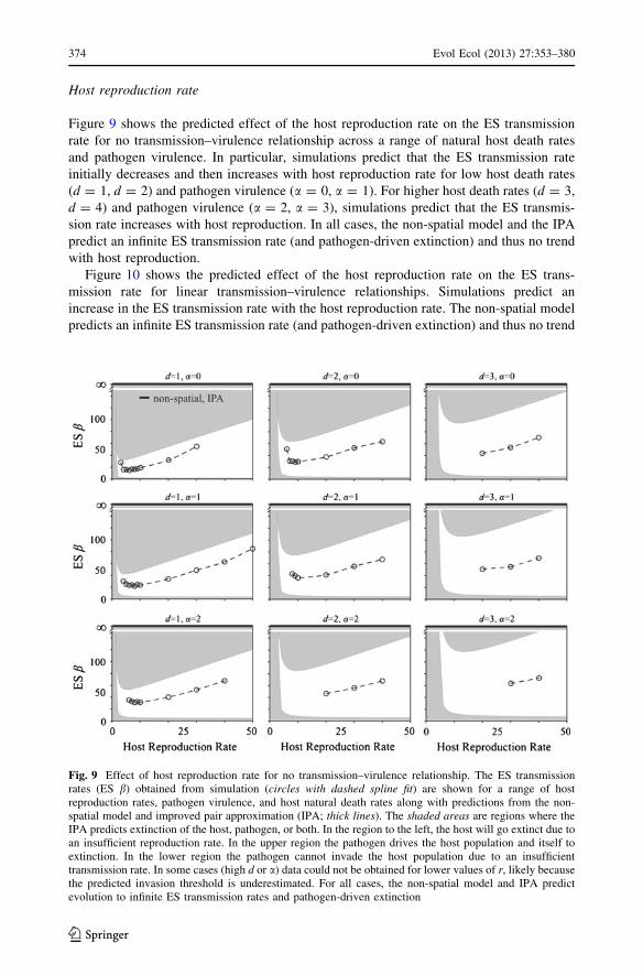
Figure 9 shows the predicted effect of the host reproduction rate on the ES transmission

rate for no transmission–virulence relationship across a range of natural host death rates

and pathogen virulence. In particular, simulations predict that the ES transmission rate

initially decreases and then increases with host reproduction rate for low host death rates

(d = 1, d = 2) and pathogen virulence (a = 0, a = 1). For higher host death rates (d = 3,

d = 4) and pathogen virulence (a = 2, a = 3), simulations predict that the ES transmis-

sion rate increases with host reproduction. In all cases, the non-spatial model and the IPA

predict an infinite ES transmission rate (and pathogen-driven extinction) and thus no trend

with host reproduction.

Figure 10 shows the predicted effect of the host reproduction rate on the ES trans-

mission rate for linear transmission–virulence relationships. Simulations predict an

increase in the ES transmission rate with the host reproduction rate. The non-spatial model

predicts an infinite ES transmission rate (and pathogen-driven extinction) and thus no trend

Fig. 9 Effect of host reproduction rate for no transmission–virulence relationship. The ES transmissionrates (ES b) obtained from simulation (circles with dashed spline fit) are shown for a range of hostreproduction rates, pathogen virulence, and host natural death rates along with predictions from the non-spatial model and improved pair approximation (IPA; thick lines). The shaded areas are regions where theIPA predicts extinction of the host, pathogen, or both. In the region to the left, the host will go extinct due toan insufficient reproduction rate. In the upper region the pathogen drives the host population and itself toextinction. In the lower region the pathogen cannot invade the host population due to an insufficienttransmission rate. In some cases (high d or a) data could not be obtained for lower values of r, likely becausethe predicted invasion threshold is underestimated. For all cases, the non-spatial model and IPA predictevolution to infinite ES transmission rates and pathogen-driven extinction

374 Evol Ecol (2013) 27:353–380

123

with host reproduction. The IPA correctly predicts an intermediate ES transmission rate for

all host reproduction rates. However, the trends with host reproduction are qualitatively

wrong, especially when the relationship is less steep and the host reproduction rate is low:

the ES transmission rate is predicted to be greater than the extinction threshold trans-

mission rate, effectively predicting pathogen-driven extinction.

Figure 11 shows the predicted effect of the host reproduction rate on the ES trans-

mission rate for concave-down transmission–virulence tradeoffs. Simulations predict an

increase in the ES transmission rate with the host reproduction rate. Though the non-spatial

model correctly predicts an intermediate transmission rate across host reproduction rates, it

predicts no trend with the host reproduction rate. The IPA correctly predicts that the ES

transmission rate varies with the host reproduction rate. Further, the predicted trends are

qualitatively similar to the trends predicted by simulation. Quantitatively, however, the

relative difference between the ES transmission rate predicted by IPA and simulations

varies depending on the steepness of transmission–virulence tradeoff as well as the host

Fig. 10 Effect of hostreproduction rate for lineartransmission–virulencerelationships. The EStransmission rates (ES b)obtained from simulation (circleswith dashed spline fit) are shownacross a range of hostreproduction rates and tradeoffsteepness, along with predictionsfrom the non-spatial model (thicksolid line) and improved pairapproximation (IPA; thin solidline). The shaded areas are as inFig. 9. Data could not beobtained for lower values of r,likely because the IPA predictedinvasion threshold isunderestimated. For all graphs,d = 1

Evol Ecol (2013) 27:353–380 375

123

reproduction rate and natural death rate. As the transmission–virulence tradeoff becomes

steeper (higher z in a = C�bz where C = 0.1) the relative difference decreases. In fact, for

the steepest tradeoff (a = 0.1�b1.7), the difference between predictions is nearly 0 across all

host reproduction rates. For less steep tradeoffs, the relative difference is highest for low

host reproduction rates, but decreases as host reproduction increases.

Host mortality

Figure 12 shows the effect of host mortality (either natural host death rate or virulence) on

the ES transmission rate for no transmission–virulence relationship. Simulations predict

that the ES transmission rate will increase with increased host mortality. However, the

factor of increase declines as the host reproduction rate increases, and for high host

reproduction rates the ES transmission rate may actually decrease. The non-spatial model

predicts an infinite ES transmission rate for all mortality rates and thus predicts no trend

with either the host natural death rate or virulence. Similarly, the IPA incorrectly predicts

an infinite ES transmission rate and pathogen-driven extinction regardless of the host

natural death rate or virulence. Thus, the ES transmission rate predicted by IPA is both

qualitatively and quantitatively inaccurate.

Figure 13 (top two panels and lower left panel) shows the effect of host mortality

(natural host death rate) on the ES transmission rate for linear transmission–virulence

Fig. 11 Effect of host reproduction rate for concave-down transmission–virulence tradeoffs. The EStransmission rates (ES b) obtained from simulation (circles with dashed spline fit, error bars shown whenlarger than data points) are shown across a range of host reproduction rates and tradeoff steepness, alongwith predictions from the non-spatial model (thick solid line) and improved pair approximation (IPA; thinsolid line). The shaded areas are as in Fig. 9

376 Evol Ecol (2013) 27:353–380

123

relationships. Simulations predict that the ES transmission rate will increase with

increased host mortality. In some cases the factor of increase is greater for low host

reproduction rates, but the trend is not consistent across relationship shapes. For some

parameter sets the IPA correctly predicts that the ES transmission rate should increase

with host death rate; however, overall the predicted trends are qualitatively and quan-

titatively inaccurate.

Figure 13 (lower right panel) also shows the effect of host mortality (natural host death

rate) on the ES transmission rate for a concave-down transmission–virulence tradeoff.

Simulations, the non-spatial model, and the IPA predict that the ES transmission rate will

increase with increased host mortality. The non-spatial model predicts the same factor of

increase in the ES transmission rate with host mortality across host reproduction rates. In

contrast, though the trends are not strong, the IPA predicts a slight decrease in the influence

of host death with host reproduction while simulations predict a slight increase with host

reproduction.

Fig. 12 Effect of host mortality on ES transmission rate for no transmission–virulence relationship. Thefactor of increase in the ES transmission rate (ES b) with a unit increase in the death rate (d; top left panela = 0 and top right panel a = 1) and virulence (a; bottom left panel d = 1 and bottom right panel d = 2)from simulations (bars) along with predictions from the non-spatial model and improved pair approximation(IPA; thick lines) is shown for a range of host reproduction rates. A value of 1 represents no change in theES b with death rate or virulence, a value greater than 1 is an increase, and a value less than 1 is a decrease.For example, the first bar in the top left graph (the d = 1–2 bar) indicates that when a = 0 the EStransmission rate is 3.5 times higher when d = 2 than when d = 1. The non-spatial model and IPA predictno change across host reproduction rates

Evol Ecol (2013) 27:353–380 377

123

References

Alizon S, Lion S (2011) Within-host parasite cooperation and the evolution of virulence. Proc R Soc LondSer B Biol Sci 278(1725):3738–3747

Anderson RM, May RM (1982) Coevolution of hosts and parasites. Parasitology 85:411–426Bauch CT (2005) The spread of infectious diseases in spatially structured populations: an invasory pair

approximation. Math Biosci 198(2):217–237Best A, Webb S, White A et al (2011) Host resistance and coevolution in spatially structured populations.

Proc R Soc Lond Ser B Biol Sci 278(1715):2216–2222Boerlijst MC, van Ballegooijen WM (2010) Spatial pattern switching enables cyclic evolution in spatial

epidemics. PLoS Comput Biol 6(12):e1001030Bonhoeffer S, Lenski RE, Ebert D (1996) The curse of the pharaoh: the evolution of virulence in pathogens

with long living propagules. Proc R Soc Lond Ser B Biol Sci 263(1371):715–721Boots M, Sasaki A (1999) ‘Small worlds’ and the evolution of virulence: infection occurs locally and at a

distance. Proc R Soc Lond Ser B Biol Sci 266(1432):1933–1938Boots M, Sasaki A (2000) The evolutionary dynamics of local infection and global reproduction in host-

parasite interactions. Ecol Lett 3(3):181–185Boots M, Hudson PJ, Sasaki A (2004) Large shifts in pathogen virulence relate to host population structure.

Science 303(5659):842–844Boots M, Kamo M, Sasaki A (2006) The implications of spatial structure within populations to the evolution

of parasites. In: Feng Z, Dieckmann U, Levin SA (eds) Disease evolution: models, concepts, and dataanalyses. American Mathematical Society, Providence, p 297

Fig. 13 Effect of host mortality on ES transmission rate for transmission–virulence relationships, linear andconcave-down tradeoffs. The factor of increase in the ES transmission rate (ES b) with an increase in thedeath rate from d = 1 to d = 2 is shown for a range of host reproduction rates and tradeoff types: threelinear and one concave down (simulation data = bars, predictions from non-spatial model = thick solidline, predictions from IPA = thin solid line). The factor of increase predicted by simulations is alwaysgreater than or equal to 1 (dashed line). For the least steep linear tradeoff, the dotted portion of the curveindicates that the IPA predicts an ES b above the extinction threshold for d = 1 or d = 2 at that hostreproduction rate

378 Evol Ecol (2013) 27:353–380

123

Bull JJ (1994) Virulence. Evolution 48(5):1423–1437Caraco T, Glavanakov S, Li SG et al (2006) Spatially structured superinfection and the evolution of disease

virulence. Theor Popul Biol 69(4):367–384Claessen D, de Roos AM (1995) Evolution of virulence in a host-pathogen system with local pathogen

transmission. Oikos 74(3):401–413Cooper VS, Reiskind MH, Miller JA et al (2002) Timing of transmission and the evolution of virulence of an

insect virus. Proc R Soc Lond Ser B Biol Sci 269(1496):1161–1165Day T (2002) Virulence evolution via host exploitation and toxin production in spore-producing pathogens.

Ecol Lett 5(4):471–476Day T (2003) Virulence evolution and the timing of disease life-history events. Trends Ecol Evol

18(3):113–118de Aguiar MAM, Rauch EM, Bar-Yam Y (2004) Invasion and extinction in the mean field approximation

for a spatial host-pathogen model. J Stat Phys 114(5/6):1417–1451de Roode JC, Yates AJ, Altizer S (2008) VIrulence–transmission trade-offs and population divergence in

virulence in a naturally occuring butterfly parasite. PNAS 105(21):7489–7494Dieckmann U, Law R (2000) Moment approximations of individual-based models. In: Dieckmann U, Law

R, Metz JAJ (eds) The geometry of ecological interactions: simplifying spatial complexity. CambridgeUniversity Press, Cambridge, pp 252–270

Eshelman CM, Vouk R, Stewart JL, Halsne E, Lindsey HA, Schneider S, Gualu M, Dean AM, Kerr B (2010)Unrestricted migration favours virulent pathogens in experimental metapopulations: evolutionarygenetics of a rapacious life history. Phil Trans R Soc B Biol Sci 365(1552):2503–2513

Ewald PW (1987) Transmission modes and evolution of the parasitism-mutualism continuum. Ann NYAcad Sci 503:295–306

Ewald PW (1993) Evolution of virulence. Sci Am 268:56–62Ewald PW (1998) The evolution of virulence and emerging diseases. J Urban Health Bull NY Acad Med

75(3):480–491Filipe JAN, Maule MM (2003) Analytical methods for predicting the behaviour of population models with

general spatial interactions. Math Biosci 183(1):15–35Frank SA (1996) Models of parasite virulence. Q Rev Biol 71(1):37–78Gandon S (1998) The curse of the pharaoh hypothesis. Proc R Soc Lond Ser B Biol Sci 265(1405):

1545–1552Gillespie DT (1977) Exact stochastic simulation of coupled chemical reactions. J Phys Chem 81(25):

2340–2361Goodnight C, Rauch E, Sayama H et al (2008) Evolution in spatial predator-prey models and the ‘‘prudent

predator’’: the inadequacy of steady-state organism fitness and the concept of individual and groupselection. Complexity 13(5):23–44

Hansen SK, Rainey PB, Haagensen JAJ et al (2007) Evolution of species interactions in a biofilm com-munity. Nature 445(7127):533–536

Harada Y, Iwasa Y (1994) Lattice population-dynamics for plants with dispersing seeds and vegetativepropagation. Res Popul Ecol 36(2):237–249

Haraguchi Y, Sasaki A (2000) The evolution of parasite virulence and transmission rate in a spatiallystructured population. J Theor Biol 203(2):85–96

Johnson CR, Boerlijst MC (2002) Selection at the level of the community: the importance of spatialstructure. Trends Ecol Evol 17(2):83–90

Johnson CR, Seinen I (2002) Selection for restraint in competitive ability in spatial competition systems.Proc R Soc Lond Ser B Biol Sci 269:655–663

Kamo M, Boots M (2004) The curse of the pharaoh in space: free-living infectious stages and the evolutionof virulence in spatially explicit populations. J Theor Biol 231(3):435–441

Kamo M, Boots M (2006) The evolution of parasite dispersal, transmission, and virulence in spatial hostpopulations. Evol Ecol 8(7):1333–1347

Kamo M, Sasaki A, Boots M (2007) The role of trade-off shapes in the evolution of parasites in spatial hostpopulations: an approximate analytical approach. J Theor Biol 244(4):588–596

Kerr B, Godfrey-Smith P (2002) Individualist and multi-level perspectives on selection in structured pop-ulations. Biol Philos 17(4):477–517

Kerr B, Neuhauser C, Bohannan BJM et al (2006) Local migration promotes competitive restraint in a host-pathogen ‘tragedy of the commons’. Nature 442(7098):75–78

Le Galliard JF, Ferriere R, Dieckmann U (2003) The adaptive dynamics of altruism in spatially hetero-geneous populations. Evolution 57(1):1–17

Levin BR, Bull JJ (1994) Short-sighted evolution and the virulence of pathogenic microorganisms. TrendsMicrobiol 2(3):76–81

Evol Ecol (2013) 27:353–380 379

123

Levin S, Pimentel D (1981) Selection of intermediate rates of increase in parasite-host systems. Am Nat117(3):308–315

Lion S, Boots M (2010) Are parasites ‘‘prudent’’ in space? Ecol Lett 13(10):1245–1255Lion S, van Baalen M (2008) Self-structuring in spatial evolutionary ecology. Ecol Lett 11(3):277–295Matsuda H, Ogita N, Sasaki A et al (1992) Statistical mechanics of population: the lattice Lotka-Volterra

model. Prog Theor Phys 88(6):1035–1049May RM, Anderson RM (1982) Parasite-host coevolution. In: Futuyma DJ, Slatkin M (eds) Coevolution.

Sinauer Associates, Inc., Sunderland, pp 186–206Messinger SM, Ostling A (2009) The consequences of spatial structure for the evolution of pathogen

transmission rate and virulence. Am Nat 174(4):441–454Morris AJ (1997) Representing spatial interactions in simple ecological models. Dissertation, University of

WarwickMosquera J, Adler FR (1998) Evolution of virulence: a unified framework for coinfection and superin-

fection. J Theor Biol 195(3):293–313Nowak MA, Sigmund K (2002) Super- and coinfection: the two extremes. In: Dieckmann U, Metz JAJ,

Sabelis MW, Sigmund K (eds) Adaptive dynamics of infectious diseases: in pursuit of virulencemanagement. Cambridge University Press, Cambridge, pp 124–149

Ohtsuka K, Konno N, Masuda N et al (2006) Phase diagrams and correlation inequalities of a three-statestochastic epidemic model on the square lattice. Int J Bifurc Chaos 16(12):3687–3693

Osnas EE, Dobson AP (2010) Evolution of virulence when transmission occurs before disease. Biol Lett6(4):505–508

Peyrard N, Dieckmann U, Franc A (2008) Long-range correlations improve understanding of the influenceof network structure on contact dynamics. Theor Popul Biol 73(3):383–394

Prado F, Kerr B (2008) The evolution of restraint in bacterial biofilms under nontransitive competition.Evolution 62(3):538–548

Rauch EM, Sayama H, Bar-Yam Y (2002) Relationship between measures of fitness and time scale inevolution. Phys Rev Lett 88(22):1–4

Roche B, Drake JM, Rohani P (2011) The curse of the Pharaoh revisited: evolutionary bi-stability inenvironmentally transmitted pathogens. Ecol Lett 14(4):569–575

Sato K, Matsuda H, Sasaki A (1994) Pathogen invasion and host extinction in lattice structured populations.J Math Biol 32(3):251–268

Slobodkin LB (1974) Prudent predation does not require group selection. Am Nat 108(963):665–678van Baalen M, Rand DA (1998) The unit of selection in viscous populations and the evolution of altruism.

J Theor Biol 193(4):631–648van Baalen M, Saebelis MW (1995) The milker-killer dilemma in spatially structured predator–prey

interactions. Oikos 74:391–400Walther BA, Ewald PW (2004) Pathogen survival in the external environment and the evolution of viru-

lence. Biol Rev 79(4):849–869Webb SD, Keeling MJ, Boots M (2007a) Spatially extended host-parasite interactions: the role of recovery

and immunity. Theor Popul Biol 71(2):251–266Webb SD, Keeling MJ, Boots M (2007b) Host–parasite interactions between the local and the non-spatial:

how and when does spatial population structure matter? J Theor Biol 249(1):140–152White PJ, Norman RA, Hudson PJ (2002) Epidemiological consequences of a pathogen having both virulent

and avirulent modes of transmission: the case of rabbit haemorrhagic disease virus. Epidemiol Infect129(3):665–677

380 Evol Ecol (2013) 27:353–380

123