The Investment Performance of Housing and “Hedonic” Spatial

Equilibrium

By

Tracey Seslen Marshall School of Business

University of Southern California

William C. Wheaton Department of Economics

MIT

Henry O. Pollakowski Center for Real Estate

MIT

DRAFT: August, 2005

The authors are indebted to CSW/FISERV, the Warren Group, and Dataquick, Inc. for the provision of data. The Authors remain fully responsible for all conclusions and analysis drawn from this research.

2

ABSTRACT This research unites the two major strands of work that exist to date in the literature on Housing Markets. The first is the notion of spatial equilibrium wherein consumers inhabiting different units are thought to be at a constant utility level. As a consequence prices “compensate” for differential “hedonic” housing attributes. The second is the application of life-cycle analysis to the determination of the “full” cost of owning housing as a financial asset. Linking the two we hypothesize that it is the “risk-adjusted annual cost of ownership” which should compensate owners for the differential consumption flows that come from various houses. To test whether this is the case we develop a unique data set for 4 US metropolitan areas that ascertains the appreciation and risk from owning housing at the ZIP code level. We then combine this with transaction based data on price levels – at the same level of geographic detail. We find that in ZIP codes with higher historic appreciation, price levels are indeed higher, but we suspect that this may represent misspecification through an identity. When we test over a shorter period for whether prices anticipate future appreciation – we get very mixed results. In nearly half of the specifications ex ante appreciation are insignificant or have the wrong sign. The results for risk are similarly disappointing. These results reinforce the doubts raised by others over whether the housing market is “efficiently” priced.

3

I. INTRODUCTION This paper connects two central ideas in the long literature on Housing markets.

The first idea, Ricardian Rent, is hundreds of years old. Ricardo [1817] hypothesized that

in equilibrium, land would absorb the advantages of location and its price would hence

exactly compensate for any and all attributes that either consumers or producers would

“value”. Following a significant expansion by Alonso [1967] and then Rosen [1974],

there have appeared hundreds of papers using the idea of spatial equilibrium to implicitly

value travel time, public goods and environmental externalities (e.g. Smith [1995], Bartik

[1987]), not to mention a host of housing attributes (e.g. Case et. al [1989], Palmquist

[1984], Brown and Rosen [1982]) . Recently there has arisen some criticism over the

empirical specification of “hedonic” models (e.g. Epple [1987], Ekeland et. al [2004]) ,

but the central theoretical premise of prices acting to “compensate” remains quite central

to much applied research.

The second strand in the housing literature is inter-temporal and deals with the

consumption of housing services over time and the investment returns contained therein.

Starting with Kearl [1979], Schwab [1982], Dougherty and Van Order [1982] economists

realized that the un-taxed nominal capital gains earned by owning housing could bestow

a major advantage to home ownership (Hamilton and Schwab [1985]). Poterba [1984] put

this idea into a rational expectations equilibrium framework and demonstrated that

unanticipated shocks to housing demand would generate anticipated patterns of future

price appreciation that would generate further increases in housing demand. After this it

was well recognized that the “user cost” of owning housing incorporated expected future

capital gains as well as implicit rent – even with trading frictions (Grossman and Laroque

[1990]).

A union of these two literatures began with a paper by Capozza and Helsley

[1990] in which the authors showed that in a Ricardian equilibrium for a growing city,

prices would have to not only compensate for location attributes but also for the

anticipated changing valuation of those attributes over time due to growth. Dipasquale

and Wheaton [1996] expounded upon this and showed how with anticipated growth,

certain locations within a city would have both high price levels and high growth in

4

Ricardian rent, while other areas would exhibit the reverse. In equilibrium, a “user cost”

measure of Rent-minus-appreciation would be exactly the same across locations.

The present paper takes this union one further step arguing that it should be Rent-

minus-appreciation-plus risk that is equilibrated across locations. Empirically, the

implication is that all hedonic equations should include the two investment dimensions of

housing – expected appreciation and risk – in addition to observable physical and

location characteristics. To the extent that such investment behavior is correlated with

measured attributes, the omission biases results.

To test these ideas empirically for the first time we undertake a several-part study.

We begin by obtaining repeat sale price indices at the ZIP-code level for 4 MSAs. These

indices span roughly 25 years (from 1979 to 2004) and reveal several conclusions. First,

virtually all ZIP codes do in fact closely follow the cyclic movements of the broader

MSA. Secondly, these cyclic movements are quite predictable as other authors have

argued (e.g. Case et. al [1989]). Thirdly, there are significant differences across ZIP

codes (within an MSA) in longer term appreciation and risk and there are consistent

patterns in which areas have higher appreciation and lower risk. Finally, there is the

expected positive simple correlation between risk and historic return across ZIP levels –

although it is generally weak.

We next produce hedonic price equations for a single year within but near the end

of those spanned by the indices (1998). We do this with thousands of transactions in each

MSA and each transaction is linked to a ZIP code. Incorporating measured risk and

appreciation measures into the hedonic equations we find the following:

1) Historic appreciation is reflected in 1998 prices in roughly the magnitude that

would be suggested by theory. This occurs in all 4 of our MSAs.

2). However, several measures of ex ante appreciation (from 1998-2004) are not

well reflected in 1998 prices – particularly when the appreciation of the last 6 years is any

different from historical.

3) Risk (which can only be measured historically) is correctly reflected in price in

only 1 of 4 MSAs.

4). Not surprisingly, risk and return are correlated particularly strongly with some

location variables and hence their omission could change the estimated impacts of those

5

variables. In our 4 cities however, this turns out not to be a problem. The impact of

location variables on house prices seems to come not from consumer’s valuing the flow

of services they produce, but rather from the fact that certain locations have higher

expected long term appreciation.

Our paper proceeds in accordance with the discussion above. In Section II we

review some theoretical literature and develop a simple model to illustrate how the

historic investment behavior of housing markets can be expected to impact current or

future consumption decisions. Section III then describes the repeat sale price indices

obtained, their behavior over time, and offers several different measures of risk and

appreciation. We present these metrics in several different ways and show that they are

highly autocorrelated over time. We also show that risk and appreciation are positively

related historically across ZIP codes and that there are strong location patterns to the

investment performance of housing

In Section IV, we describe the data used to construct our hedonic equations in

each MSA. We use a number of specifications with and without investment variables, but

all appreciation measures are historically based over the full time period. We compare

results across MSAs and find that the point estimates for historic appreciation are

reasonable according to several theoretical perspectives.

In Section V we argue that the encouraging results of the previous section could

be due to an identity, and remove this possible specification error by determining if

anticipated future appreciation is reflected in prices. Our results in this case are quite poor

and raise the prospect that ex ante investment performance is not well priced. We draw

some conclusions which reinforce the literature on housing market inefficiency and

suggest further research.

II. HOW SHOULD RISK AND APPRECIATION BE PRICED IN HOUSING?

In this section we develop a simple model of housing consumption to illustrate

how the expected (and possibly historic) appreciation and risk characteristics of housing

markets determine the consumption decision. In short run equilibrium, with supply

largely fixed, the impact on desired consumption will be directly translated into housing

6

prices. In long run equilibrium, some of these impacts will be tempered by supply

response, but with less than perfect supply elasticity, they will still hold qualitatively.

We begin with a 2 period model with two forms of consumption -- housing (a

durable, h) and a numeraire (non-durable, c). In the first period, the individual has total

wealth W0, and must decide how much to allocate of this in the next period between

riskless asset b and housing wealth ph. In the second period the return on b is R which is

known with certainty. The appreciation on housing is H is known with uncertainty and

comes from the probability distribution of the change in p over the second period.1

Efficient capital markets allow the individual to finance its numeraire consumption in the

second period with the total return on wealth: phH + Rb.

In this framework, the individual has preferences represented by the CARA utility

function with no intermediate consumption. Returns on housing, H, are normally

distributed with mean Hµ and variance 2Hσ . The individual maximizes:

hacehcU α−−−=),( (1)

subject to

bphW +=0 and

RbphHc += Solving the maximization

][max][max )( hRbphHahac eEeE αα −+−−− −=− , we get optimal housing expenditure

2*

H

H

aa

Rph

σ

αµ +−= (2)

Thus optimal housing expenditure will increase when the appreciation on housing

is expected to be greater, will decrease as other investments have higher returns and will

decrease with the greater the risk associated with homeownership. It is purely a function

of the moments of housing returns, and wealth effects do not come into play.

7

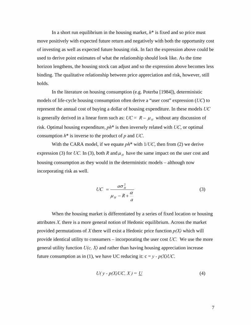
In a short run equilibrium in the housing market, h* is fixed and so price must

move positively with expected future return and negatively with both the opportunity cost

of investing as well as expected future housing risk. In fact the expression above could be

used to derive point estimates of what the relationship should look like. As the time

horizon lengthens, the housing stock can adjust and so the expression above becomes less

binding. The qualitative relationship between price appreciation and risk, however, still

holds.

In the literature on housing consumption (e.g. Poterba [1984]), deterministic

models of life-cycle housing consumption often derive a “user cost” expression (UC) to

represent the annual cost of buying a dollar of housing expenditure. In these models UC

is generally derived in a linear form such as: UC = R – Hµ without any discussion of

risk. Optimal housing expenditure, ph* is then inversely related with UC, or optimal

consumption h* is inverse to the product of p and UC.

With the CARA model, if we equate ph* with 1/UC, then from (2) we derive

expression (3) for UC. In (3), both R and Hµ have the same impact on the user cost and

housing consumption as they would in the deterministic models – although now

incorporating risk as well.

UC

aR

a

H

H

αµ

σ

+−=

2

(3)

When the housing market is differentiated by a series of fixed location or housing

attributes X, there is a more general notion of Hedonic equilibrium. Across the market

provided permutations of X there will exist a Hedonic price function p(X) which will

provide identical utility to consumers – incorporating the user cost UC. We use the more

general utility function U(c, X) and rather than having housing appreciation increase

future consumption as in (1), we have UC reducing it: c = y - p(X)UC.

U( y - p(X)UC, X ) = U (4)

8

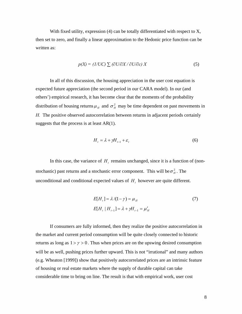
With fixed utility, expression (4) can be totally differentiated with respect to X,

then set to zero, and finally a linear approximation to the Hedonic price function can be

written as:

p(X) = (1/UC) ∑ (∂U/∂X / ∂U/∂c) X (5)

In all of this discussion, the housing appreciation in the user cost equation is

expected future appreciation (the second period in our CARA model). In our (and

others’) empirical research, it has become clear that the moments of the probability

distribution of housing returns Hµ and 2Hσ may be time dependent on past movements in

H. The positive observed autocorrelation between returns in adjacent periods certainly

suggests that the process is at least AR(1).

ttt HH εγλ ++= −1 (6)

In this case, the variance of tH remains unchanged, since it is a function of (non-

stochastic) past returns and a stochastic error component. This will be 2Hσ . The

unconditional and conditional expected values of tH however are quite different.

HtHE µγλ =−= )1/(][ (7)

Httt HHHE µγλ ′=+= −− 11 ]|[

If consumers are fully informed, then they realize the positive autocorrelation in

the market and current period consumption will be quite closely connected to historic

returns as long as 01 >> γ . Thus when prices are on the upswing desired consumption

will be as well, pushing prices further upward. This is not “irrational” and many authors

(e.g. Wheaton [1999]) show that positively autocorrelated prices are an intrinsic feature

of housing or real estate markets where the supply of durable capital can take

considerable time to bring on line. The result is that with empirical work, user cost

9

measures may be generated using recent or historic movements of the housing returns

data without necessarily violating economic rationality.

III. THE INVESTMENT PERFORMANCE OF ZIP-LEVEL HOUSING

MARKETS.

Empirical evidence on the risk, appreciation and predictability of housing prices

at the metropolitan level has been well-documented, starting with Case and Shiller

[1989]. Using transactions and other administrative data from four major metropolitan

areas, their study showed strong positive autocorrelation in returns over short intervals;

an increase in housing prices in the current period predicted an increase ¼ to ½ as large

in the following period. Similar results from a larger sample of metropolitan areas were

estimated in Capozza, Hendershott, and Mack [2004] and Seslen [2004]. No study, as of

yet, has extended this type of analysis to the sub-metropolitan level.

In this section, we use weighted repeat-sales housing price indices provided to us

by Case Shiller Weiss/FISERV at the ZIP code level to examine a series of questions.

These include whether ZIP level housing prices behave closely with their MSA aggregate

index or whether there are wide differences. We next present a set of time series metrics

to characterize each ZIP series. These include simple risk and appreciation measures as

well as the parameters of a univariate model (estimated separately for each ZIP). The data

cover four MSAs: Boston, Chicago, Phoenix, and San Diego. In choosing these areas,

we have attempted to create a sample representing a diverse set of demographic,

geographic, and housing market-related conditions.

The Boston metropolitan area covers 249 ZIP codes from 1982 through 2002,

Chicago comprises 152 ZIP codes from 1987 through 2002; Phoenix includes 164 ZIP

codes spanning 1988 to 2002, and San Diego covers 86 ZIP codes starting in 1975. In

the final version of our empirical model, the data were kept or dropped based on three

conditions: the length of the time series itself, the proximity of the zip code to the center

of the MSA, and the availability of other data needed to carry out the later stages of our

analysis. For Boston, we confined our sample to those ZIP codes within the I-495

beltway; outside that area, it could be argued that Boston is not the primary center of

economic “pull” on housing prices, and we did not want that possibility to cloud our

10

results. For the other three MSAs, attenuation of the sample size was primarily due to the

lack of corresponding transactions data.

The final sample resulted in 109 observations for Boston, 51 for Chicago, 80 for

Phoenix, and 42 for San Diego. For purposes of discussion, price levels are deflated using

the (urban) consumer price index. The risk and appreciation measures used in estimation

are all calculated in current dollars.

As can been seen in Figure 1, housing prices across the four MSAs were behaving

quite differently from one another over the last two decades. While Boston and San

Diego were experiencing significant boom-bust cycles, Chicago and Phoenix were

progressing through substantially less volatile paths.

Figure 1

MSA Real Price SeriesData reported quarterly, baseline at 1995q1

0

20

40

60

80

100

120

140

1975

:1

1980

:1

1985

:1

1990

:1

1995

:1

2000

:1

Pric

e In

dex

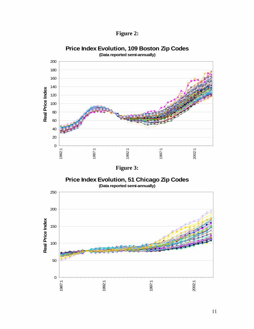
Boston-Worcester MSA Chicago MSA Phoenix-Mesa MSA San Diego MSA In Figures 2 through 5, we have graphed the price series for every ZIP in each of

the four MSAs again in constant dollars. Within Boston and San Diego, the ZIP-level

series follow one another quite closely, while in Chicago and Phoenix, they exhibit

greater divergence from one another, particularly towards the end of the sample period.

From first glances, it would appear that “a rising tide raises all boats.”

11

Figure 2:

Price Index Evolution, 109 Boston Zip Codes(Data reported semi-annually)

0

20

40

60

80

100

120

140

160

180

20019

82:1

1987

:1

1992

:1

1997

:1

2002

:1

Rea

l Pric

e In

dex

Figure 3:

Price Index Evolution, 51 Chicago Zip Codes(Data reported semi-annually)

0

50

100

150

200

250

1987

:1

1992

:1

1997

:1

2002

:1

Rea

l Pric

e In

dex

12

Figure 4:

Price Index Evolution, 80 Phoenix Zip Codes(Data reported semi-annually)

0

50

100

150

200

25019

88:1

1993

:1

1998

:1

2003

:1

Rea

l Pri

ce In

dex

Figure 5:

Price Index Evolution, 42 San Diego Zip Codes(Data reported semi-annually)

0

20

40

60

80

100

120

140

160

180

200

1974

:1

1979

:1

1984

:1

1989

:1

1994

:1

1999

:1

2004

:1

Rea

l Pri

ce In

dex

It is possible to more formally characterize the distribution of ZIP series for each

MSA. In Appendix 1, we provide the ZIP level quantile distribution of (current dollar) risk

and appreciation for each market. Table 1 below summarizes those results and shows that for

most markets, 90% of the ZIP codes have raw risk and appreciation that spans two or three

percentage points or alternatively lies with 1.5% either side of the MSA mean.

Table 1: distribution of ZIP statistics (current $)

(90-percent inter-quartile range shown for risk and return)

MSA MSA Return Return Risk

Boston 8.5 7.5 – 9.5 8.5 – 11.5

Chicago 6.5 5.0 – 9.5 2.5 – 5.0

Phoenix 5.0 3.8 – 7.0 2.5 – 5.0

S. Diego 7.6 6.5 – 8.5 7.7 – 10.0

In one sense the range breadth in the distribution of return and risk across ZIPs is a

measure of the degree to which each MSA is “spatially integrated”. If all ZIP codes are close

substitutes and demand very elastic across areas then presumably ZIP codes would behave

quite closely. Conversely, if there is lower spatial demand elasticity and ZIP codes are quite

differentiated then the variation in behavior would be greater. By this standard, Boston and

San Diego are the more “integrated” while Chicago and Phoenix are less “integrated”. In all

these markets there is a significant positive correlation between risk and appreciation –

although this will be discussed in more detail later.

As an alternative to using simple descriptive statistics to examine the behavior of ZIP

level price series we also estimate a basic autoregressive model for each series – and then

examine the spread in the parameter distribution of this model across the ZIPs. The rationale

for this is based on the idea that if some component of price variation is expected,

individuals do not need to receive compensation for it (in the form of a “risk premium”)

because the variation does not make them worse off. In a predictable market where

participants observe the autoregressive and mean reverting behavior, appreciation should be

the underlying trend in the series and true “risk” is the component of price variation that is

unexpected. If there were little expected variation in housing prices (which seems unlikely

14

here given Figures 2-5), then the use of either measure would lead to similar results and

conclusions.

The model we use is adapted from Capozza, Hendershott, and Mack [2004]2, and has

three parameters of interest: one representing the autocorrelation of housing prices over

time, one representing the degree of mean reversion in housing prices, and the last being the

structural (or equilibrium) trend around which housing prices oscillate. The root MSE of the

model will be of interest as a measure of the degree of unexplainable variation in housing

prices and of course the trend will represent underlying return.

In the CHM model, the change in housing prices from today to tomorrow is a

function of the change in housing prices from yesterday to today, and the deviation of

housing prices from an equilibrium price level, P*, which can change over time, and is

estimated in a first-stage regression of price on various MSA-level economic and

demographic characteristics. Due to the lack of time series economic data at the ZIP code

level, and in name of simplicity, we eliminate the first stage, and assume that each ZIP’s

prices deviate around a constant trend. This gives the following specification:

εββ +−+−=− −++ )ln(ln)ln(lnlnln *21112 ttttt PPPPPP (8)

where: bTrendaeP +=*

In our model, housing price changes are measured over an interval of one year;

however, the housing price index itself is measured every six months. So we end up with an

overlapping of intervals. With this, the above equation translates to:

εγγγγ +++−+=− −++ TrendPPPPP ttttt 3211102 ln)ln(lnlnln , (9)

where: a20 βγ = , 22 βγ −= , and b23 βγ = .

The parameter 1γ (or equivalently, - 1β ) measures autocorrelation in the housing

series and 2γ , mean reversion. Estimation of the latter will allow the backing out of a and b,

where b is the underlying ZIP trend.

15

In our time series model, the parameter space allows for four possible outcomes with

regard to housing market cyclic behavior. With mean reversion ( 02 <β ) and

autocorrelation ( 1β ) greater than one, prices diverge in an oscillating fashion. With mean

reversion, and autocorrelation less than one, prices converge with oscillations. With no

mean reversion ( 02 ≥β ) and autocorrelation greater than one, prices diverge with no

oscillations. Finally, with no mean reversion and autocorrelation less than one (or with

mean reversion and very small values of 1β ), prices converge with no oscillations.3

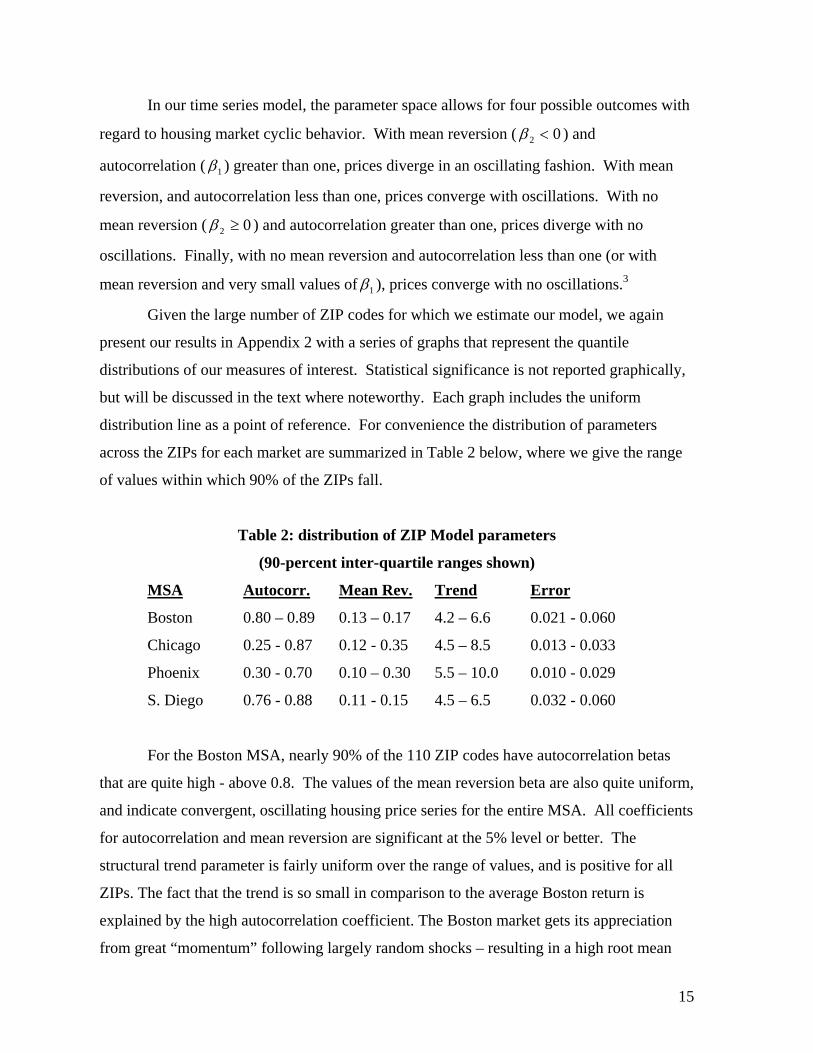
Given the large number of ZIP codes for which we estimate our model, we again

present our results in Appendix 2 with a series of graphs that represent the quantile

distributions of our measures of interest. Statistical significance is not reported graphically,

but will be discussed in the text where noteworthy. Each graph includes the uniform

distribution line as a point of reference. For convenience the distribution of parameters

across the ZIPs for each market are summarized in Table 2 below, where we give the range

of values within which 90% of the ZIPs fall.

Table 2: distribution of ZIP Model parameters

(90-percent inter-quartile ranges shown)

MSA Autocorr. Mean Rev. Trend Error

Boston 0.80 – 0.89 0.13 – 0.17 4.2 – 6.6 0.021 - 0.060

Chicago 0.25 - 0.87 0.12 - 0.35 4.5 – 8.5 0.013 - 0.033

Phoenix 0.30 - 0.70 0.10 – 0.30 5.5 – 10.0 0.010 - 0.029

S. Diego 0.76 - 0.88 0.11 - 0.15 4.5 – 6.5 0.032 - 0.060

For the Boston MSA, nearly 90% of the 110 ZIP codes have autocorrelation betas

that are quite high - above 0.8. The values of the mean reversion beta are also quite uniform,

and indicate convergent, oscillating housing price series for the entire MSA. All coefficients

for autocorrelation and mean reversion are significant at the 5% level or better. The

structural trend parameter is fairly uniform over the range of values, and is positive for all

ZIPs. The fact that the trend is so small in comparison to the average Boston return is

explained by the high autocorrelation coefficient. The Boston market gets its appreciation

from great “momentum” following largely random shocks – resulting in a high root mean

16

squared error. The fit of the time series model to the Boston data is still good, with a

minimum R-squared of 0.63. Over 90% of the observations fall between 0.8 and the

maximum of 0.96.4

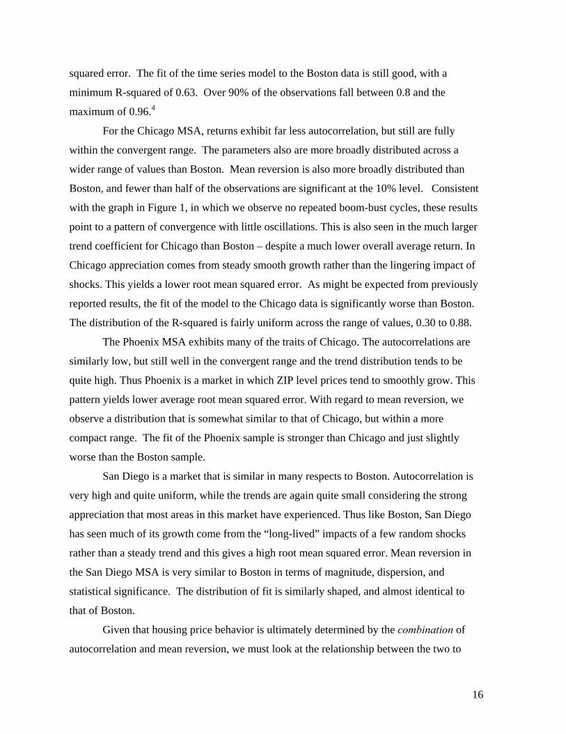
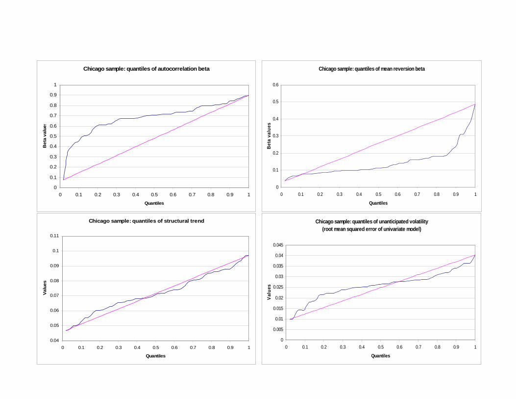
For the Chicago MSA, returns exhibit far less autocorrelation, but still are fully

within the convergent range. The parameters also are more broadly distributed across a

wider range of values than Boston. Mean reversion is also more broadly distributed than

Boston, and fewer than half of the observations are significant at the 10% level. Consistent

with the graph in Figure 1, in which we observe no repeated boom-bust cycles, these results

point to a pattern of convergence with little oscillations. This is also seen in the much larger

trend coefficient for Chicago than Boston – despite a much lower overall average return. In

Chicago appreciation comes from steady smooth growth rather than the lingering impact of

shocks. This yields a lower root mean squared error. As might be expected from previously

reported results, the fit of the model to the Chicago data is significantly worse than Boston.

The distribution of the R-squared is fairly uniform across the range of values, 0.30 to 0.88.

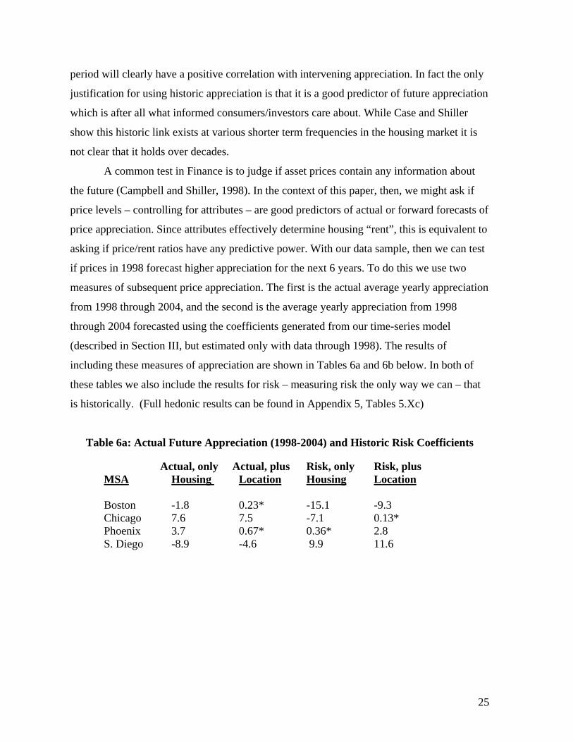
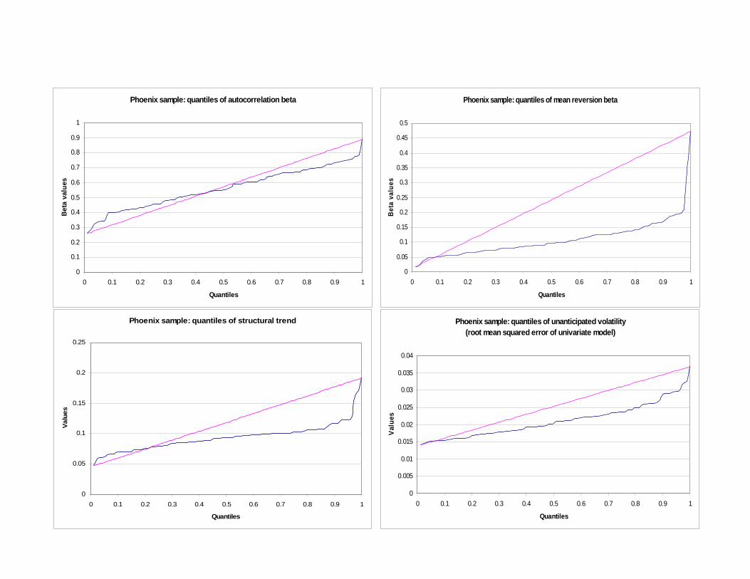
The Phoenix MSA exhibits many of the traits of Chicago. The autocorrelations are

similarly low, but still well in the convergent range and the trend distribution tends to be

quite high. Thus Phoenix is a market in which ZIP level prices tend to smoothly grow. This

pattern yields lower average root mean squared error. With regard to mean reversion, we

observe a distribution that is somewhat similar to that of Chicago, but within a more

compact range. The fit of the Phoenix sample is stronger than Chicago and just slightly

worse than the Boston sample.

San Diego is a market that is similar in many respects to Boston. Autocorrelation is

very high and quite uniform, while the trends are again quite small considering the strong

appreciation that most areas in this market have experienced. Thus like Boston, San Diego

has seen much of its growth come from the “long-lived” impacts of a few random shocks

rather than a steady trend and this gives a high root mean squared error. Mean reversion in

the San Diego MSA is very similar to Boston in terms of magnitude, dispersion, and

statistical significance. The distribution of fit is similarly shaped, and almost identical to

that of Boston.

Given that housing price behavior is ultimately determined by the combination of

autocorrelation and mean reversion, we must look at the relationship between the two to

17

complete our analysis – which we do with the figures in Appendix 3. Once again, we

observe strong similarities within the Boston-San Diego and Chicago-Phoenix pairs. Across

all four MSAs, there is a tendency toward lower levels of mean reversion ( 2β or - 1γ closer to

zero) in ZIP codes with higher levels of autocorrelation. In Boston and San Diego, the

observations are very tightly bunched, and the relationship is fairly subtle. For Chicago and

Phoenix, the observations are highly dispersed and the relationship is extremely pronounced.

In these two markets, we see quite a few ZIP codes that would fall into the parameter region

where there is convergence with no oscillations, while we see no such observations in the

other two MSAs.

In Section II we argued that a full equilibrium requires that the overall risk adjusted

cost of owning a home compensate for the utility flow of services. Thus we would expect to

find that “rent” (price level times opportunity cost of capital) minus expected appreciation

plus the value of risk must compensate for service flow. In this equilibrium, this is

equivalent to having risk equal the service flow minus rent plus expected appreciation. Thus

holding service flow and prices fixed (if that is possible), we expect to find a positive

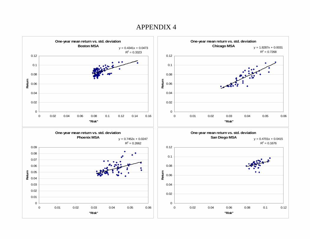
(partial) relationship between risk and appreciation. and in Appendix 4 we examine if there

are in fact such a positive relationships across the ZIP codes of our 4 MSAs. We do this with

a series of scatterplots and accompanying regressions

The first panel in Appendix 4 shows the relationship between “raw” appreciation and

risk – the average, one-year log difference in the price index and the standard deviation of

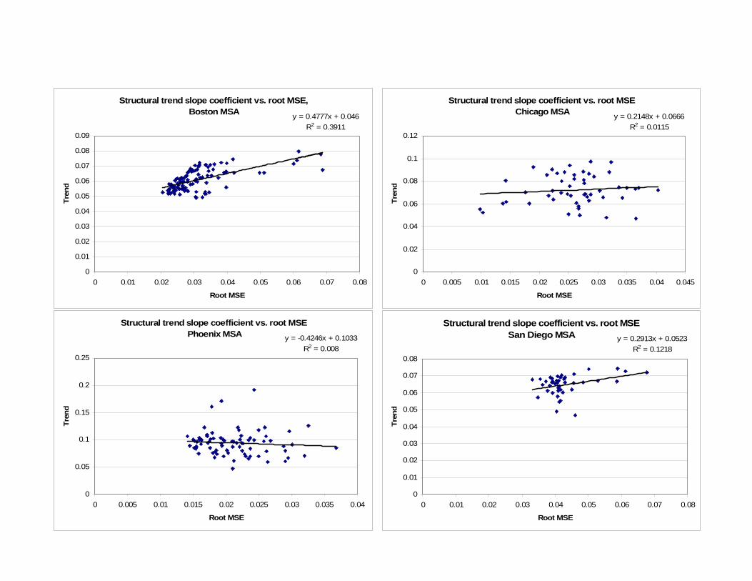
that difference over the entire time-series interval. In the bottom panel, we substitute

estimated appreciation and risk (the equilibrium slope coefficient and root MSE of the time

series model, respectively) for the raw measure.

The strongest positive relationship between risk and appreciation can be found with

the raw measures in Phoenix, where we observe a correlation of around 0.85. Phoenix is

followed by Boston at 0.58 and Phoenix at 0.52. The worst of the four is San Diego, in

which the data exhibit a wide range of returns within a much narrower band of risk.

Looking at our alternative measures of risk and return, we generally observe a lower degree

of correlation than with the raw measure. Only Boston shows an improvement using the

estimated values. Thus with respect to these historic performance, it does seem that ZIPs

behave somewhat as an inter-temporal spatial equilibrium would demand.

18

Not only is there predictability over time in ZIP level investment performance, there

is also cross-sectional predictability. In each market we can run regressions between the ZIP

level location variables that we will include shortly, and risk or return. To illustrate the

spatial patterns of investment performance Table 3 presents cross section regressions of five

main ZIP characteristics on investment performance. We do this for appreciation before and

after 1998 – the date at which we will be examining Hedonic prices.

Table 3: Cross Section predicted House Price Appreciation Boston Chicago Phoenix San Diego Variable -98 / +98 -98 /+98 -98 /+98 -98 /+98 R2 0.81 / 0.81 0.88 / 0.72 0.66 / 0.64 0.88 / 0.85 Nonwhite 0.01 / 0.03 -0.005* / -0.01* -0.03 / -0.016* -0.006 / 0.13 Distance -0.11 / -0.05 -0.19 / -0.27 -0.31 / -0.32 0.02 / -0.09 Distance2 0.12 / .04 0.19 / 0.37 0.69 / 0.70 -0.08 / 0.14 Ocean dist. n/a n/a n/a -2.1 / 0.01* Median. inc. 0.0001* / .03 -0.009* / -0.01* 0.001* / .0003* 0.0002* / -4.2 All coefficients significant at 5% except those with an *.

The first observation from Table 3 is that ZIP appreciation is quite predictable. In all

markets but San Diego, for example, ZIPs at farther distances from the urban center have

less appreciation. The impact of median income and the percentage of nonwhite residents is

inconsistent across metropolitan areas in both sign and significance.

The second observation is that in Chicago and Phoenix, these patterns are quite

stable both before and after 1998. In Boston and San Diego however, they change quite

significantly. In these latter two cities appreciation in the last 6 years is not at all similar to

that which happened in the 15-20 years prior to 1998.

IV: INCORPORATING HISTORIC INVESTMENT PERFORMANCE INTO

HEDONIC EQUATIONS.

The data employed to estimate the hedonic regressions came from a variety of

sources. The transactions data and housing unit characteristics were obtained from two real

estate information clearing houses: The Warren Group and Dataquick, Inc. The former

provided data for the Boston area, while the latter provided data for the other three MSAs.

19

Data were initially limited to owner-occupied, single-family detached units. Further filtering

led to the discarding of units with essential data missing, or values believed to be data

reporting or recording errors. Homes with sale prices below $20,000 (Boston) and $10,000

(Chicago, Phoenix, and San Diego) were also discarded as possible indications of non-arms-

length sales, possible data reporting/recording errors, or otherwise being non-representative

of “normal” housing prices in our MSAs. All data were from 1998. For the Boston MSA,

housing characteristics included the number of bedrooms, the number of bathrooms, interior

square footage, lot size, and the year in which the house was built. Observations were

further discarded if the number of bedrooms or bathrooms was less than one. The lot size

was bounded between 0.02 and 10 acres. After filtering, we were left with 19,848

observations. For the Chicago MSA, housing characteristics were limited to number of

bathrooms, interior square footage, and lot size. Observations were discarded if the number

of bathrooms was less than one and no upper limit was placed on lot size. The final dataset

contained 12,799 observations. Transaction data for the Phoenix MSA included the number

of bathrooms, the number of total rooms, interior square footage, lot size, year built, and

whether the house had a garage or pool. In this dataset, houses with “three-quarter” baths

(containing a toilet and shower) were grouped together with those containing the next

highest whole number of bathrooms. As with the Chicago MSA, no upper bound was placed

on the lot size. The transactions data for San Diego contained the number of bedrooms,

number of bathrooms, interior square footage, and whether the house had a garage or pool.

Lot size was missing from over 40% of the observations, and therefore was ultimately

omitted from the regression analysis. The final dataset contained 34,511 observations. In

addition to those filters listed for Boston, square footage was bounded from below at a value

of 300. The final dataset contained 13,970 observations.

Among the location attributes used in our hedonic specification, population density,

median income, rate of homeownership and percentage nonwhite were obtained from the

2000 Decennial Census gazetteer and summary files. With the exception of median income,

the location attributes were calculated using various other data from the census files, i.e.

total population, total land area, total housing units, number of owner-occupied units, and

total nonwhite population. The distance from the city center and the distance to the ocean

(San Diego only) were generated using Mapquest internet mapping software.5

20

For the Boston area only, we also included a set of variables measuring educational

quality and crime, two location factors which one would expect to be strongly capitalized

into housing values. Educational quality is measured by 1998 Massachusetts

Comprehensive Assessment System (MCAS) combined scores.6 The MCAS is a

standardized test that is administered in a variety of grades as a means of measuring public

school performance. All students in the participating grades must take the exam, regardless

of disability status or level of English proficiency. Scores are reported for “all students” and

“regular students” (non-disabled and English proficient). In our analysis, we include the

district-level scores for regular students in Grade 10 only. MCAS data were obtained from

the Massachusetts Department of Education website.7

Data on crime were broken down into two categories, property crime and violent

crime. Data for the city of Boston for 1998, broken down by neighborhood, was obtained

from the Boston Police Office of Media Relations.8 Data on all other towns came from the

Massachusetts Crime Reporting Unit website.9 Crime rates are presented as a per capita

measure. Crimes incurred on college campuses are recorded separately from the towns in

which they are located, and are not included in our measure. Data on crime and educational

quality were not included in the analysis of the other three MSAs.10

The final variables included in the hedonic model measure risk and appreciation. In

our analysis, we use two different sets of measures, each based off of the CSW/FISERV

dataset described earlier. In the first instance, we use raw measures of risk and average

historic appreciation – the log difference in the housing price index over a one-year interval,

averaged (by ZIP code) over the entire duration of the time series, and the standard deviation

of that average. In the second instance, return is measured as the slope coefficient on the

structural trend from our time series model, while “risk” is the root mean squared error of

the model. To carry out our initial analysis, we run six different hedonic specifications for

each of the four MSAs: 1) prices against housing characteristics alone, 2) prices against

housing characteristics with the addition of price appreciation and risk, 3) prices against

housing and trend and root mean squared error, 4) prices against housing characteristics and

location variables, 5) prices against housing characteristics, location variables with price

appreciation and risk, and 6), prices against housing characteristics, location variables and

21

trend and root mean squared error. In all of our specifications, we regress the log of prices

against a linear list of right hand side variables (Cropper [1988], Case et. al [1991])

The results of these hedonic equations are presented in full in Appendix 5. For each

city there is a table of summary statistics, followed by a table of the combined regression

results. Our primary concern is with the additional role that the various risk and return

measures add to the equations so to that effect we present Tables 4a, and 4b. We then

discuss the results for each city in turn.

Table 4a: Historic Appreciation Coefficients

Average, only Average plus Trend, only Trend, plus MSA Housing Location Housing Location Boston 25.4 10.6 35.2 14.4 Chicago 12.8 11.6 9.4 6.5 Phoenix 13.3 5.1 .1* -.8* S. Diego 17.6 -2.6 15.7 1.8

Table 4b: Historic Risk Coefficients Risk, only Risk, plus RMSE, only RMSE, plus MSA Housing Location Housing Location Boston -27.1 -11.2 -15.9 -3.8 Chicago -21.2 -10.1 -4.4 -5.2 Phoenix 0.6 2.5 -2.7 3.1 S. Diego -3.8 11.0 6.2 9.0 All coefficients significant at 5% except those with *.

Boston. The basic equation with only housing characteristics has an R2 of 0.53.

Almost all coefficients except the indicators for 3 and 4 bedrooms are significant. This

result is often found when total interior square feet is controlled for; homes with many small

rooms are not as valued. When the investment variables are added, the R2 jumps quite

dramatically to 0.64 in the case where raw risk and appreciation are used or 0.62 when trend

and root mean squared error are the metrics. Both variables are very significant, and have the

correct sign.

22

When the location variables are added into the hedonic equation, the R2 rises to 0.69.

It is important to note that the equation with location variables and no investment

performance metrics has about the same R2 as the equation with just the investment metrics.

As established earlier, there is a high degree of collinearity between the investment metrics

and the location variables.

Chicago. The basic equation for Chicago, containing only housing characteristics

has a somewhat lower R2 than Boston at 0.44. Unlike Boston, adding in our investment

metrics increases the explanatory power of the equation only modestly, to an R2 of around

0.47. The appreciation variable has the hypothesized positive sign, and is smaller in

magnitude to Boston when measured either as return or trend.

When the locational attributes are added, the R2 increases from 0.47 to 0.61. The

appreciation and trend metrics now are much closer in point estimate to the Boston results,

and the risk metrics remain significantly negative in sign.

Phoenix. Phoenix, with a richer array of structural variables, has a “base” R2 of

0.70. When we add in raw risk and average appreciation the R2 increases only to 0.72, and

barely at all with trend and root mean squared error. Raw appreciation is quite significant,

trend appreciation less so. The raw risk metric has the wrong sign.

Once location variables are added to the equation the R2 increases only modestly,

from 0.70 to 0.76 (Appendix Table 5.4b column 4). When in turn the investment metrics are

added, R2 increases less than one percentage point. With the location variables included both

risk measures perform poorly.

San Diego. The San Diego results are similar to those in Boston. San Diego has a

“base” R2 of 0.54. When the investment metrics are added the R2 increases to 0.57. Both

average appreciation and risk have the correct signs only when entered in raw form and only

without the location variables.

With the addition of the location variables, the R2 increases 8 to 10 percentage

points. The raw appreciation variable no longer has a positive coefficient, and both

appreciation coefficients are significantly smaller in magnitude. The risk coefficients both

have positive signs and have increased in value.

In summary, the hedonic equations produce quite reasonable results without the

investment variables – results that seem typical with other studies. The inclusion of historic

23

appreciation, measured either raw or with the trend variable is almost always highly

significant and with a large positive coefficient. The risk metric, however, has more mixed

results. Only in Boston and Chicago does this variable consistently have the expected

significant and negative impact (measured either raw or as root mean squared error). In

many of the other markets, its impact is positive on price and in many cases this effect is

significant. At this time we have no explanation for the absence of risk-pricing in the

markets outside of Boston and Chicago.

The magnitude of the coefficients also should be judged against the theory of Section

II. The point estimates in Table 3a suggest in exchange for a 1% increase in annual

appreciation (for 25 years – or effectively forever) owners are willing to pay between 10%

and 20% more for a unit (with the same flow of utility-based services). If there are no

liquidity constraints we can think of this 1% yearly increase in appreciation as an income

flow which must be discounted. In perpetuity we should be willing to pay 1/discount rate for

that. By this reasoning a coefficient of 10 to 20 is just in the correct ballpark.

We can also examine equation (4) in more detail. There if we take the percentage

derivative of p with respect to a unit change in Hµ we get 1/ )(a

RHαµ +− . In real terms

housing appreciates a bit more than the real interest rate R, but this expression actually is

dominated by the CARA coefficient ratio aα . This ratio is the same as the ratio of housing

to “other” expenditure and might have a value on average of say 0.2. By this formulation we

would get a coefficient in a log price regression that is smaller – around 5.0.

When we turn to the risk coefficients, things obviously become much more

complicated. When we examine equation (4) we would get a percentage derivative of price

with respect to the “value” of risk (the product: 2Haσ ) that is minus 1 over that value. From

an investment perspective, in liquid financial markets, the “value” of the risk in housing

should be the difference between the total return to housing and the risk free return (R). With

3% real appreciation and say a 6% rent payment and 2% real R, we would say that the

product should be between 5% and 10%. One over that would give a regression coefficient

of between -10 and -20. Interestingly that is almost exactly the case in Boston and Chicago,

24

but not in the other cities, where the coefficient most often has the wrong sign. Further

investigation of the data may be needed to resolve this issue.

A second objective of the paper is to ascertain if the inclusion of the investment

performance metrics changes any other coefficients that are included in such equations – in

particular for variables that represent location attributes. Here the most pronounced results

occur in Boston where it was possible to collect some data on public services that

overlapped nicely with ZIP codes. The inclusion of the investment metrics had a very

inconsistent impact on the importance of crime and no impact on the valuation of school

quality. For the other MSA and attributes we turn to Table 5.

Table 5: Impact of Historic Investment Metrics on Hedonic Location Coefficients Boston Chicago Phoenix San Diego Variable WO / W WO / W WO / W WO / W Nonwhite -0.40 / -0.19 -0.52 / -0.40 -0.79 / -0.69 -0.66 / -0.71 Distance -1.6 / -0.86 0.24* / 1.1 -2.2 / -0.53 -1.14 / -0.96 School qual. 0.0026 / 0.0024 na na na Med. inc. 0.80 / 0.65 1.2 / 1.1 0.42 / 0.39 0.63 / 0.61 All coefficients significant at 5% except those with an *.

In Boston, the inclusion of the investment metrics modestly reduces the negative

impact of a ZIP’s racial makeup, but in the other cities the coefficients hold up. Likewise, in

all four MSAs, the impact of ZIP median income is largely left intact with the inclusion of

the investment metrics. The most significant impact of the investment variables is on the

distance to the city center. Thus it would appear that the utility flow valuations of

neighborhood income, race and school quality hold up reasonably well when the investment

performance of these areas is included – despite the observed correlations between these

variables and investment performance (Table 3).

V. EX ANTE INVESTMENT PERFORMANCE AND HOUSE PRICES

There is a significant problem with using historic appreciation in a housing price

equation in which price is measured near the end of the period over which appreciation is

calculated. By construction, ZIP areas that differ in prices randomly at the beginning of the

25

period will clearly have a positive correlation with intervening appreciation. In fact the only

justification for using historic appreciation is that it is a good predictor of future appreciation

which is after all what informed consumers/investors care about. While Case and Shiller

show this historic link exists at various shorter term frequencies in the housing market it is

not clear that it holds over decades.

A common test in Finance is to judge if asset prices contain any information about

the future (Campbell and Shiller, 1998). In the context of this paper, then, we might ask if

price levels – controlling for attributes – are good predictors of actual or forward forecasts of

price appreciation. Since attributes effectively determine housing “rent”, this is equivalent to

asking if price/rent ratios have any predictive power. With our data sample, then we can test

if prices in 1998 forecast higher appreciation for the next 6 years. To do this we use two

measures of subsequent price appreciation. The first is the actual average yearly appreciation

from 1998 through 2004, and the second is the average yearly appreciation from 1998

through 2004 forecasted using the coefficients generated from our time-series model

(described in Section III, but estimated only with data through 1998). The results of

including these measures of appreciation are shown in Tables 6a and 6b below. In both of

these tables we also include the results for risk – measuring risk the only way we can – that

is historically. (Full hedonic results can be found in Appendix 5, Tables 5.Xc)

Table 6a: Actual Future Appreciation (1998-2004) and Historic Risk Coefficients Actual, only Actual, plus Risk, only Risk, plus MSA Housing Location Housing Location Boston -1.8 0.23* -15.1 -9.3 Chicago 7.6 7.5 -7.1 0.13* Phoenix 3.7 0.67* 0.36* 2.8 S. Diego -8.9 -4.6 9.9 11.6

26

Table 6b: Forecast Future Appreciation (1998-2004) and Historic Risk Coefficients1 Forecast, only Forecast, plus Risk, only Risk, plus MSA Housing Location Housing Location Boston 21.0 7.0 -2.6 -3.1 Chicago -10.4 0.23* 13.8 -2.2 Phoenix 3.4 1.6 4.8 4.2 S. Diego 8.0 -0.71* 4.7 9.8 All coefficients significant at 5% except those with an *.

The results in these tables are quite disappointing. A quick look back at Figures 2

through 5 shows that the period from 1998-2004 saw both a great deal of housing price

appreciation, and if anything a widening gap between the appreciation of individual ZIP

areas. Despite this fact, the predictive power of prices with respect to appreciation is very

poor. In the first two columns of Tables 6a, 5 of 8 of the appreciation coefficients are either

insignificant or of the incorrect sign! It is very questionable if actual future appreciation was

anticipated by price (to rent) levels in 1998. This is very much worse than the results we

obtained using actual historic appreciation in Table 4a, where all coefficients were

appropriate. This suggests that our concern over misspecification was probably justified.

It might be argued that future appreciation can not always be anticipated by past data

- particularly given the results of Table 3, and in Boston and San Diego. That said, prices (if

forward looking) should still pick up the predictable part of actual future appreciation – in

Table 6b. This story seems to hold for Boston (where the forecasted impacts now have the

correct signs) but not San Diego, with only one correctly-signed investment coefficient.

Likewise, in Chicago, where appreciation had quite similar patterns after 1998 to before, the

forecasted appreciation signs all are wrong. With results using forecasted appreciation nearly

as poor as those using actual appreciation, we are forced to conclude that the market is

largely inefficient in pricing forward growth. The risk results are equally poor whether

paired with actual or forecasted growth, with 10 out of 16 total coefficients showing an

incorrect sign.

In terms of further research, there are clear priorities. We need to expand the number

of location variables to possibly include environmental measures, and to obtain the crime

and school data for the remaining MSAs. Quite possibly the absence of these important

27

variables is altering our results. For the moment, however, we conclude that while the

housing market is quite predictable, across locations, this predictability is not efficiently

priced into current price levels.

1 We ignore the possibility that there might be uncertainty in the received consumption flow of housing, h, and focus on just the financial uncertainty embedded in H. 2 Heretofore referred to as the CHM model 3 See CHM [2004] Figure 1. 4 In the interest of space, the graphs of the R-squared distributions have been omitted. They are available upon request. 5 Distance was measured based on the most efficient driving route between the center of the ZIP code and the center of the city proper. 6 This is the sum of scores from English/Language Arts, Mathematics, and Science and Technology 7 http://www.doe.mass.edu/mcas/results.html 8 The neighborhood data conform very closely, if not perfectly, to ZIP code boundaries. Assigning neighborhood-specific crime values to the various ZIP codes within the Boston city limits proved very important, due to the overall city size and strong variation in crime rates across locations 9 http://www.ucrstats.com/ 10 Boston was a very convenient “test case” for the explanatory power and “proxy value” of education and crime statistics, since 1) every town has its own school district and police force, and 2) the ZIP codes contained within those towns never cross town borders. In the other three MSAs, ZIP codes often contain more than one school district or police jurisdiction, making it very difficult to pinpoint the district/jurisdiction governing the particular housing unit in the sample.

References

Alonso, W. Location and Land Use, (Cambridge, MA: Harvard University Press, 1964). Bartik, Timothy. “The Estimation of Demand Parameters in Hedonic Price Models, Journal of Political Economy, 95 (1987) 172-183. Brown, James, and Harvey Rosen. “On the Estimation of Structural Hedonic Price Models”, Econometrica, 50 (1982) 765-768. Campbell, John, and Shiller, R.J. "Valuation Ratios and the Long Run Stock Market Outlook” Journal of Portfolio Management, (Winter, 1998) 11-26. Capozza, Dennis and Bob Helsley. "The Stochastic City", Journal of Urban Economics, 28 (1990) 187-203. Capozza, Dennis, Hendershott, Patric, and Charlotte Mack. “An Anatomy of Price Dynamics in Illiquid Markets: Analysis and Evidence from Local Housing Markets,” Real Estate Economics, 32 (2004) 1-21. Case, Bradford, Henry O. Pollakowski, and Susan M. Wachter. “On Choosing among Housing Price Index Methodologies,” AREUEA Journal, 19 (1991), 286-307. Case, K.E., and Shiller, R.J. "The Efficiency of the Market for Single Family Homes," American Economic Review, 79 (1989) 125-137. Cropper, Maureen, Leland Deck and Kenneth McConnell. “On the Choice of Functional Form for Hedonic Price Functions.” Review of Economics and Statistics. 70 (1988) 688-675. DiPasquale, D. and Wheaton, W.C. Urban Economics and Real Estate Markets, Prentice Hall, New Jersey (1996). Dougherty, A., and R. Van Order. "Inflation, Housing Costs and the Consumer Price Index", American Economic Review, 72 (1982). Ekeland, Ivar, James Heckman, and Lars Nesheim. “Identification and Estimation of Hedonic Models”, Journal of Political Economy, 112 (2004 forthcoming). Epple, Dennis. “Hedonic Prices and Implicit Markets: Estimating Demand and Supply Functions for Differentiated Products”, Journal of Political Economy, 95 (1987) 59-80. Grossman, Sandford, and Guy Laroque. “Asset Pricing and Optimal Portfolio Choice in the Presence of Illiquid Durable Consumption Goods”, Econometrica, 58 (1990) 25-51. Hamilton, B. and R. Schwab, "Expected Price Appreciation in Urban Housing Markets," Journal of Urban Economics, 23 (1985).

28

Kearl, J.R. "Inflation, Mortgages and Housing", Journal of Political Economy, 87 (1979). Palmquist, Raymond. “Estimating the Demand for the Characteristics of Housing”, Review of Economics and Statistics, 66 (1984) 394-404. Poterba, J. M. "Tax Subsidies to Owner-Occupied Housing: An Asset-Market Approach," Quarterly Journal of Economics, 99 (1984) 729-752. Ricardo, D. On the Principles of Political Economy and Taxation, 1817. Rosen, Sherwin. “Hedonic Prices and Implicit Markets; Product Differentiation in Pure Competition”, Journal of Political Economy, 82 (1974) 35-55. Schwab, R.M. "Inflationary Expectations and the Demand for Housing", American Economic Review, 72 (1982). Seslen, Tracey N. “Housing Price Dynamics and Household Mobility Decisions,” mimeo, USC Marshall School of Business (2004). Smith, V. Kerry, and Ju-Chin Huang. “Can Markets Value Air Quality? A Meta-Analysis of Hedonic Property Value Models.” Journal of Political Economy, 103 (1995) 209-227. Wheaton, William. “Real Estate Cycles: Some Fundamentals.” Real Estate Economics, 27 (1999) 122-222.

29

Boston sample: quantiles of raw 1-year return

0.065

0.07

0.075

0.08

0.085

0.09

0.095

0.1

0.105

0.11

0 0.1 0.2 0.3 0.4 0.5 0.6 0.7 0.8 0.9 1

Quantiles

Valu

es

Chicago sample: quantiles of raw 1-year return

0.04

0.05

0.06

0.07

0.08

0.09

0.1

0.11

0 0.1 0.2 0.3 0.4 0.5 0.6 0.7 0.8 0.9 1

Quantiles

Valu

es

Boston sample: quantiles of raw 1-year risk

0

0.02

0.04

0.06

0.08

0.1

0.12

0.14

0.16

0 0.1 0.2 0.3 0.4 0.5 0.6 0.7 0.8 0.9 1

Quantiles

Valu

es

Chicago sample: quantiles of raw 1-year risk

0.02

0.025

0.03

0.035

0.04

0.045

0.05

0.055

0.06

0 0.1 0.2 0.3 0.4 0.5 0.6 0.7 0.8 0.9 1

Quantiles

Valu

es

APPENDIX 1

Phoenix sample: quantiles of raw 1-year return

0.03

0.04

0.05

0.06

0.07

0.08

0.09

0 0.1 0.2 0.3 0.4 0.5 0.6 0.7 0.8 0.9 1

Quantiles

Valu

es

San Diego sample: quantiles of raw 1-year return

0.05

0.055

0.06

0.065

0.07

0.075

0.08

0.085

0.09

0.095

0.1

0 0.1 0.2 0.3 0.4 0.5 0.6 0.7 0.8 0.9 1

Quantiles

Valu

es

Phoenix sample: quantiles of raw 1-year risk

0.02

0.025

0.03

0.035

0.04

0.045

0.05

0.055

0.06

0 0.1 0.2 0.3 0.4 0.5 0.6 0.7 0.8 0.9 1

Quantiles

Valu

es

San Diego sample: quantiles of raw 1-year risk

0.07

0.075

0.08

0.085

0.09

0.095

0.1

0.105

0.11

0 0.1 0.2 0.3 0.4 0.5 0.6 0.7 0.8 0.9 1

Quantiles

Valu

es

Boston sample: quantiles of autocorrelation beta

0

0.1

0.2

0.3

0.4

0.5

0.6

0.7

0.8

0.9

1

0 0.1 0.2 0.3 0.4 0.5 0.6 0.7 0.8 0.9 1

Quantiles

Bet

a va

lues

Boston sample: quantiles of mean reversion beta

0

0.05

0.1

0.15

0.2

0.25

0 0.1 0.2 0.3 0.4 0.5 0.6 0.7 0.8 0.9 1

Quantiles

Beta

val

ues

Boston sample: quantiles of structural trend

0.04

0.045

0.05

0.055

0.06

0.065

0.07

0.075

0.08

0.085

0 0.1 0.2 0.3 0.4 0.5 0.6 0.7 0.8 0.9 1

Quantiles

Valu

es

Boston sample: quantiles of unanticipated volatility (root mean squared error of univariate model)

0.01

0.02

0.03

0.04

0.05

0.06

0.07

0.08

0 0.1 0.2 0.3 0.4 0.5 0.6 0.7 0.8 0.9 1

Quantiles

Valu

es

APPENDIX 2

Chicago sample: quantiles of autocorrelation beta

0

0.1

0.2

0.3

0.4

0.5

0.6

0.7

0.8

0.9

1

0 0.1 0.2 0.3 0.4 0.5 0.6 0.7 0.8 0.9 1

Quantiles

Bet

a va

lues

Chicago sample: quantiles of mean reversion beta

0

0.1

0.2

0.3

0.4

0.5

0.6

0 0.1 0.2 0.3 0.4 0.5 0.6 0.7 0.8 0.9 1

Quantiles

Beta

val

ues

Chicago sample: quantiles of structural trend

0.04

0.05

0.06

0.07

0.08

0.09

0.1

0.11

0 0.1 0.2 0.3 0.4 0.5 0.6 0.7 0.8 0.9 1

Quantiles

Valu

es

Chicago sample: quantiles of unanticipated volatility (root mean squared error of univariate model)

0

0.005

0.01

0.015

0.02

0.025

0.03

0.035

0.04

0.045

0 0.1 0.2 0.3 0.4 0.5 0.6 0.7 0.8 0.9 1

Quantiles

Valu

es

Phoenix sample: quantiles of autocorrelation beta

0

0.1

0.2

0.3

0.4

0.5

0.6

0.7

0.8

0.9

1

0 0.1 0.2 0.3 0.4 0.5 0.6 0.7 0.8 0.9 1

Quantiles

Beta

val

ues

Phoenix sample: quantiles of mean reversion beta

0

0.05

0.1

0.15

0.2

0.25

0.3

0.35

0.4

0.45

0.5

0 0.1 0.2 0.3 0.4 0.5 0.6 0.7 0.8 0.9 1

Quantiles

Beta

val

ues

Phoenix sample: quantiles of structural trend

0

0.05

0.1

0.15

0.2

0.25

0 0.1 0.2 0.3 0.4 0.5 0.6 0.7 0.8 0.9 1

Quantiles

Valu

es

Phoenix sample: quantiles of unanticipated volatility (root mean squared error of univariate model)

0

0.005

0.01

0.015

0.02

0.025

0.03

0.035

0.04

0 0.1 0.2 0.3 0.4 0.5 0.6 0.7 0.8 0.9 1

Quantiles

Valu

es

San Diego sample: quantiles of autocorrelation beta

0.7

0.75

0.8

0.85

0.9

0.95

0 0.1 0.2 0.3 0.4 0.5 0.6 0.7 0.8 0.9 1

Quantiles

Beta

val

ues

San Diego sample: quantiles of mean reversion beta

0

0.02

0.04

0.06

0.08

0.1

0.12

0.14

0 0.1 0.2 0.3 0.4 0.5 0.6 0.7 0.8 0.9 1

Quantiles

Beta

val

ues

San Diego sample: quantiles of structural trend

0

0.01

0.02

0.03

0.04

0.05

0.06

0.07

0.08

0 0.1 0.2 0.3 0.4 0.5 0.6 0.7 0.8 0.9 1

Quantiles

Valu

es

San Diego sample: quantiles of unanticipated volatility (root mean squared error of univariate model)

0.03

0.035

0.04

0.045

0.05

0.055

0.06

0.065

0.07

0 0.1 0.2 0.3 0.4 0.5 0.6 0.7 0.8 0.9 1

Quantiles

Valu

es

Boston Sample: Autocorrelation vs. Mean Reversion

0

0.05

0.1

0.15

0.2

0.25

0 0.1 0.2 0.3 0.4 0.5 0.6 0.7 0.8 0.9 1

Autocorrelation beta

Mea

n re

vers

ion

beta

(red

uced

form

)

Chicago sample: Autocorrelation vs. Mean Reversion

0

0.1

0.2

0.3

0.4

0.5

0.6

0 0.1 0.2 0.3 0.4 0.5 0.6 0.7 0.8 0.9 1

Autocorrelation beta

Mea

n re

vers

ion

beta

(red

uced

form

)

Phoenix Sample: Autocorrelation vs. Mean Reversion

0

0.05

0.1

0.15

0.2

0.25

0.3

0.35

0.4

0.45

0.5

0 0.1 0.2 0.3 0.4 0.5 0.6 0.7 0.8 0.9 1

Autocorrelation beta

Mea

n re

vers

ion

beta

(red

uced

form

)

San Diego Sample: Autocorrelation vs. Mean Reversion

0

0.02

0.04

0.06

0.08

0.1

0.12

0.14

0 0.1 0.2 0.3 0.4 0.5 0.6 0.7 0.8 0.9 1

Autocorrelation beta

Mea

n re

vers

ion

beta

(red

uced

form

)

APPENDIX 3

One-year mean return vs. std. deviationBoston MSA y = 0.4341x + 0.0473

R2 = 0.3323

0

0.02

0.04

0.06

0.08

0.1

0.12

0 0.02 0.04 0.06 0.08 0.1 0.12 0.14 0.16

"Risk"

Ret

urn

One-year mean return vs. std. deviation Chicago MSA y = 1.8287x + 0.0031

R2 = 0.7268

0

0.02

0.04

0.06

0.08

0.1

0.12

0 0.01 0.02 0.03 0.04 0.05 0.06

"Risk"

Ret

urn

One-year mean return vs. std. deviation Phoenix MSA y = 0.7452x + 0.0247

R2 = 0.2662

0

0.01

0.02

0.03

0.04

0.05

0.06

0.07

0.08

0.09

0 0.01 0.02 0.03 0.04 0.05 0.06

"Risk"

Retu

rnAPPENDIX 4

One-year mean return vs. std. deviation San Diego MSA y = 0.4701x + 0.0415

R2 = 0.1676

0

0.02

0.04

0.06

0.08

0.1

0.12

0 0.02 0.04 0.06 0.08 0.1 0.12

"Risk"

Retu

rn

Structural trend slope coefficient vs. root MSE, Boston MSA y = 0.4777x + 0.046

R2 = 0.3911

0

0.01

0.02

0.03

0.04

0.05

0.06

0.07

0.08

0.09

0 0.01 0.02 0.03 0.04 0.05 0.06 0.07 0.08

Root MSE

Tren

d

Structural trend slope coefficient vs. root MSE Chicago MSA y = 0.2148x + 0.0666

R2 = 0.0115

0

0.02

0.04

0.06

0.08

0.1

0.12

0 0.005 0.01 0.015 0.02 0.025 0.03 0.035 0.04 0.045

Root MSE

Tren

d

Structural trend slope coefficient vs. root MSE Phoenix MSA y = -0.4246x + 0.1033

R2 = 0.008

0

0.05

0.1

0.15

0.2

0.25

0 0.005 0.01 0.015 0.02 0.025 0.03 0.035 0.04

Root MSE

Tren

d

Structural trend slope coefficient vs. root MSE San Diego MSA y = 0.2913x + 0.0523

R2 = 0.1218

0

0.01

0.02

0.03

0.04

0.05

0.06

0.07

0.08

0 0.01 0.02 0.03 0.04 0.05 0.06 0.07 0.08

Root MSE

Tren

d

Table 5.1 -- Variable definitions (housing and locational attributes)

log of sale price natural log of the sale pricebuilt 19XX-19YY indicator variable = 1 if the home was built during the given interval# bedroom(s) indicator variable = 1 if the home contained the designated number of bedrooms# bathrooms(s) indicator variable = 1 if the home contained the designated number of bathrooms# total room(s) indicator variable = 1 if the home contained the designated number of total roomsinterior square feet total interior square footagelot size total exterior square footage, in acrespool indicator variable = 1 if the house has a swimming poolgarage indicator variable = 1 if the house has a garageMCAS score Massachusetts Comprehensive Assessment System score, by zip. Regular

students in the 10th grade only. Range is between 600 and 840. violent crime rate incidence of murder, rape, assault, etc. per 1000 populationproperty crime rate incidence of burglary, larceny, etc. per 1000 populationdistance to city center distance in miles from the center of the zip code to the center of the MSApopulation density number of residents per square miledistance to ocean distance in miles to the nearest shoreline, via the fastest driving routeownership rate number of owner-occupied housing units divided by total units.percent nonwhite fraction of the zip population that is nonwhitelog of median income natural log of the median zip household income

APPENDIX 5

Table 5.2a -- Descriptive Statistics for the Boston Hedonic Sample

N = 19848Mean Std. Dev. Min Max

log of sale price 12.3152 0.5591 9.9035 15.0393built 1960-1980 0.2106 0.4077 0 1built 1940-1960 0.2558 0.4363 0 1built 1900-1940 0.2509 0.4335 0 1built pre-1900 0.0687 0.2530 0 11 bedroom 0.0075 0.0863 0 12 bedrooms 0.1253 0.3310 0 13 bedrooms 0.4939 0.5000 0 14 bedrooms 0.3075 0.4615 0 11 bathroom 0.2450 0.4301 0 11.5 bathrooms 0.2382 0.4260 0 12 bathrooms 0.1630 0.3694 0 12.5 bathrooms 0.2475 0.4316 0 1interior square ft. 1917.35 888.34 375.00 14241.00lot size 0.5185 0.6837 0.0211 9.9565MCAS score 701.78 24.1870 646.00 744.00violent crime rate 0.0025 0.0033 0 0.0129property crime rate 0.0190 0.0116 0 0.0480dist. to city center/100 0.2083 0.0989 0.0284 0.4597population density/10000 3.1050 2.9842 0.2631 23.6767ownership rate 0.7103 0.1501 0.2706 0.9563non white status 0.1142 0.1173 0.0077 0.9431log of median income 11.1274 0.3018 10.2010 11.9440nominal return 1982-2004 0.0849 0.0068 0.0715 0.1070std. dev. 1982-2004 0.0884 0.0083 0.0784 0.1447structural trend 0.0596 0.0062 0.0490 0.0798root mean sq. error 0.0293 0.0068 0.0206 0.0688nominal return 1998-2004 0.1150 0.0136 0.0914 0.1713forecasted return 1998-2004 0.0318 0.0084 0.0025 0.0532std. dev. 1982-1998 0.0894 0.0084 0.0793 0.1463

Table 5.2b: Comparison of coefficients, with and without risk and return. Dependent variable: ln(sale price)

Boston (1) (2) (3) (4) (5) (6)Housing attributes Housing attributes Housing attributes Housing attributes Full model with Full model with

only and raw risk/return with estimated and locational char. raw risk/return estimated risk/returnrisk/return

Built 1960-1980 0.0945 *** 0.0206 *** 0.0288 *** -0.04683 *** -0.0419 *** -0.0442 ***(0.0080) (0.0074) (0.0076) (0.0071) (0.0071) (0.0071)

Built 1940-1960 0.1287 *** -0.0248 *** -0.0145 * -0.11033 *** -0.1134 *** -0.1162 ***(0.0092) (0.0086) (0.0088) (0.0084) (0.0083) (0.0083)

Built 1900-1940 0.0731 *** -0.0460 *** -0.0703 *** -0.14939 *** -0.1455 *** 0.1501 ***(0.0101) (0.0092) (0.0096) (0.0090) (0.0089) (0.0089)

Built pre-1900 0.0198 -0.0741 *** -0.0905 *** -0.17962 *** -0.1743 *** -0.1775 ***(0.0143) (0.0131) (0.0135) (0.0125) (0.0123) (0.0124)

1 bedroom -0.1176 *** -0.1341 *** -0.1249 *** -0.16702 *** -0.1531 *** -0.1586 ***(0.0343) (0.0327) (0.0333) (0.0325) (0.0325) (0.0322)

2 bedrooms -0.0527 *** -0.0715 *** -0.0592 *** -0.08557 *** -0.0788 *** -0.0789 ***(0.0179) (0.0157) (0.0160) (0.0148) (0.0146) (0.0146)

3 bedrooms -0.0120 -0.0263 ** -0.0078 -0.0284 ** -0.0244 ** -0.0218 *(0.0158) (0.0138) (0.0140) (0.0129) (0.0128) (0.0127)

4 bedrooms -0.0049 -0.0057 0.0151 -0.01333 -0.0115 -0.0071(0.0153) (0.0134) (0.0136) (0.0126) (0.0124) (0.0124)

1 bathroom -0.5418 *** -0.3451 *** -0.3891 *** -0.26762 *** -0.2497 *** -0.2528 ***(0.0151) (0.0133) (0.0136) (0.0126) (0.0124) (0.0124)

1.5 bathrooms -0.3567 *** -0.2271 *** -0.2559 *** -0.181383 *** -0.1674 *** -0.169 ***(0.0141) (0.0122) (0.0126) (0.0115) (0.0113) (0.0113)

2 bathrooms -0.3838 *** -0.2522 *** -0.2858 *** -0.2086 *** -0.1949 *** -0.1991 ***(0.0145) (0.0127) (0.0131) (0.0119) (0.0117) (0.0117)

2.5 bathrooms -0.1468 *** -0.0926 *** -0.0936 *** -0.08157 *** -0.0738 *** -0.0728 ***(0.0122) (0.0105) (0.0109) (0.0099) (0.0098) (0.0098)

interior square feet 0.0003 *** 0.0003 *** 0.0003 *** 0.0003 *** 0.0003 *** 0.0002 ***(0.0000) (0.000) (0.0000) (0.0000) (0.0000) (0.0000)

sq. feet squared -1.56e-08 *** -1.53e-08 *** -1.39e-08 *** -1.11e-08 *** -1.20e-08 *** -1.13e-08 ***(2.35e-09) (2.39e-09) (2.45e-09) (2.50e-09) (2.54e-09) (2.54e-09)

lot size in acres 0.1361 *** 0.1575 *** 0.2243 *** 0.08388 *** 0.1001 *** 0.1 ***(0.0103) (0.0100) (0.0109) (0.0096) (0.0095) (0.0096)

lot size squared -0.0168 *** -0.0183 *** -0.0271 *** -0.01077 *** -0.0123 *** -0.0124 ***(0.0020) (0.0019) (0.0022) (0.0016) (0.0016) (0.0017)

distance to -1.6375 *** -0.8395 *** -0.6087 ***city center/100 (0.1233) (0.1536) (0.1417)

distance squared 1.0947 *** 0.5157 ** 0.2023(0.2179) (0.2437) (0.2298)

Population density/10000 0.00033 0.0116 *** 0.0019(0.0020) (0.0020) (0.0020)

homeownership rate -0.82599 *** -0.5683 *** -0.6867 ***(0.0366) (0.0400) (0.0372)

percent nonwhite -0.40788 *** -0.1889 *** -0.3083 ***(0.0301) (0.0336) (0.0363)

log of median income 0.80755 *** 0.6524 *** 0.6935 ***(0.0230) (0.0245) (0.0239)

MCAS score 0.0026 *** 0.0025 *** 0.0027 ***(regular students only) (0.0002) (0.0002) (0.0002)

violent crime rate 1.439 2.617 ** -0.9227(1.174) (1.203) (1.234)

property crime rate -0.0258 0.3979 0.8805 **(0.3247) (0.3318) (0.3334)

1-year return 25.75 *** 10.49 ***(0.4907) (0.8103)

1-year risk -27.49 *** -11.58 ***(0.4933) (0.6731)

structural trend 35.35 *** 14.48 ***(0.5569) (0.7390)

root MSE -15.89 *** -3.876 ***(0.5143) (0.7297)

R-squared 0.5266 0.6438 0.6177 0.6886 0.6956 0.6947

N 19848 19848 19848 19848 19848 19848

Robust std. errors in parentheses. *, **, and *** represent statistical significance at the 10%, 5%, and 1% levels, respectively.

Table 5.2c: Comparison of coefficients, historic risk and actual or predicted return '98-'04. Dependent variable: ln(sale price)

Boston (1) (2) (3) (4)Housing attributes Full model with Housing attributes Full model with

historic risk historic risk historic risk historic riskactual return '98-'04 actual return '98-'04 predicted return predicted return

distance to -1.9860 *** -1.379 ***city center/100 (0.1296) (0.1284)

distance squared 1.7690 *** 0.8858 ***(0.2223) (0.2247)

Population density/10000 0.0103 *** 0.0069 ***(0.0021) (0.0021)

homeownership rate -0.5855 *** -0.5502 ***(0.0402) (0.0399)

percent nonwhite -0.1435 *** -0.1703 ***(0.0332) (0.0330)

log of median income 0.6644 *** 0.6009 ***(0.0258) (0.0250)

MCAS score 0.0024 *** 0.0026 ***(regular students only) (0.0002) (0.0002)

violent crime rate 4.944 *** 2.041 *(1.185) (1.210)

property crime rate -0.2844 0.5181(0.3279) (0.3313)

1-year average return -1.811 *** -0.2453 21.29 *** 7.108 ***(0.4877) (0.5021) (0.4611) (0.5199)

1-year historic risk -15.91 *** -9.327 *** -2.59 *** -3.154 ***(0.8882) (0.9112) (0.5251) (0.8258)

R-squared 0.5909 0.6929 0.6359 0.6960

N 19848 19848 19848 19848

Robust std. errors in parentheses. *, **, and *** represent statistical significance at the 10%, 5%, and 1% levels, respectively.The above regressions all include the housing attributes found in Table 5.2b.These coefficients have been suppressed for visual clarity.

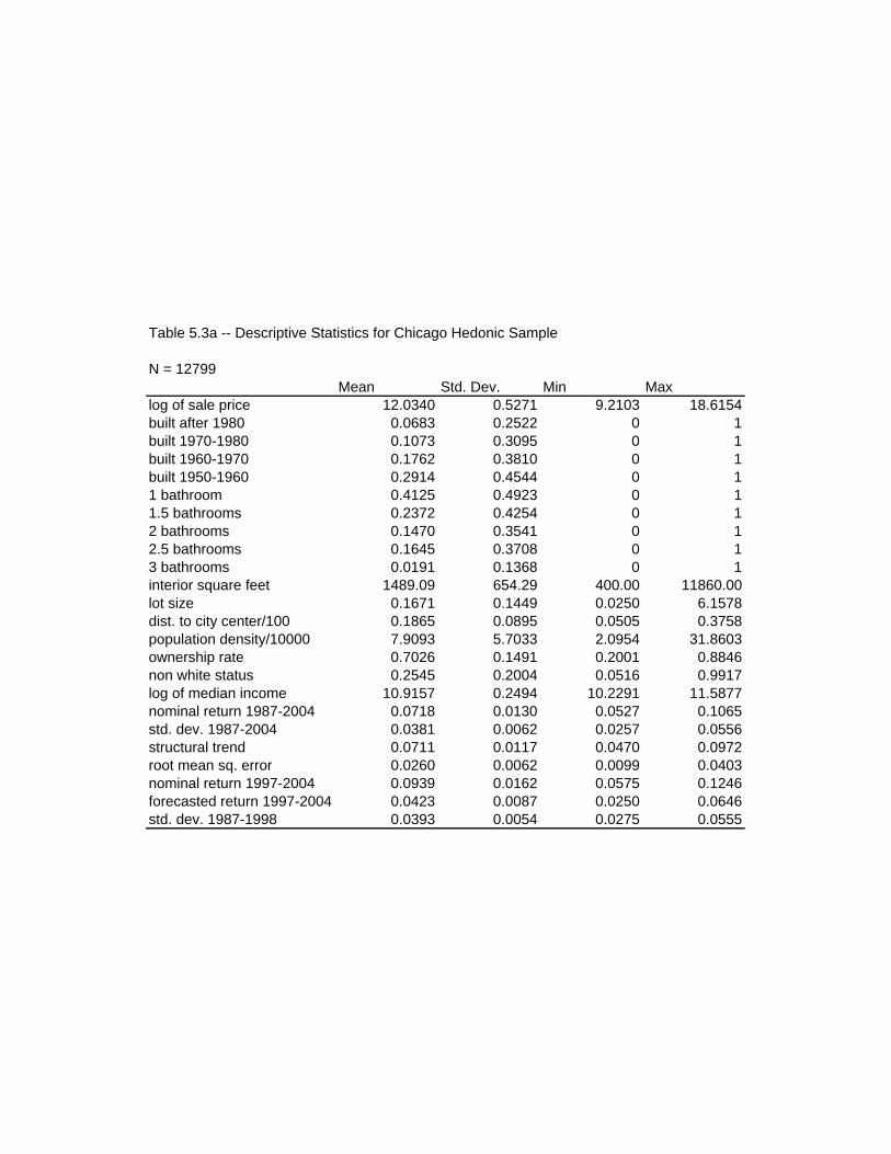
Table 5.3a -- Descriptive Statistics for Chicago Hedonic Sample

N = 12799Mean Std. Dev. Min Max

log of sale price 12.0340 0.5271 9.2103 18.6154built after 1980 0.0683 0.2522 0 1built 1970-1980 0.1073 0.3095 0 1built 1960-1970 0.1762 0.3810 0 1built 1950-1960 0.2914 0.4544 0 11 bathroom 0.4125 0.4923 0 11.5 bathrooms 0.2372 0.4254 0 12 bathrooms 0.1470 0.3541 0 12.5 bathrooms 0.1645 0.3708 0 13 bathrooms 0.0191 0.1368 0 1interior square feet 1489.09 654.29 400.00 11860.00lot size 0.1671 0.1449 0.0250 6.1578dist. to city center/100 0.1865 0.0895 0.0505 0.3758population density/10000 7.9093 5.7033 2.0954 31.8603ownership rate 0.7026 0.1491 0.2001 0.8846non white status 0.2545 0.2004 0.0516 0.9917log of median income 10.9157 0.2494 10.2291 11.5877nominal return 1987-2004 0.0718 0.0130 0.0527 0.1065std. dev. 1987-2004 0.0381 0.0062 0.0257 0.0556structural trend 0.0711 0.0117 0.0470 0.0972root mean sq. error 0.0260 0.0062 0.0099 0.0403nominal return 1997-2004 0.0939 0.0162 0.0575 0.1246forecasted return 1997-2004 0.0423 0.0087 0.0250 0.0646std. dev. 1987-1998 0.0393 0.0054 0.0275 0.0555

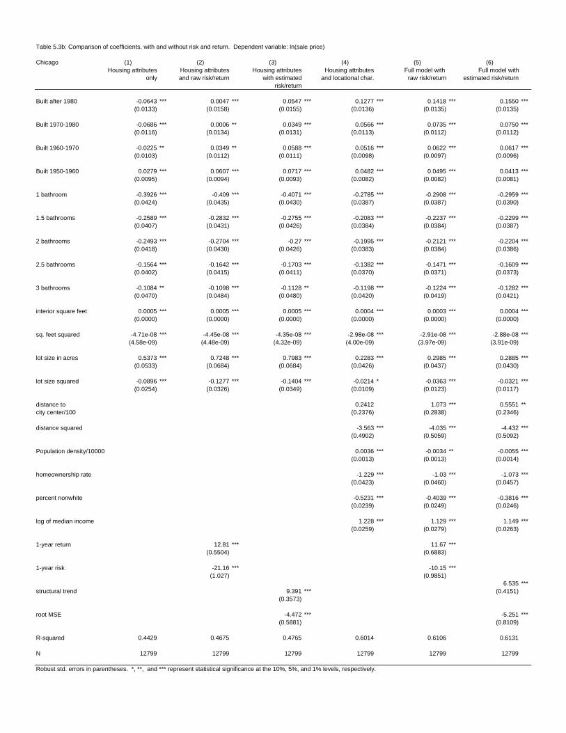
Table 5.3b: Comparison of coefficients, with and without risk and return. Dependent variable: ln(sale price)

Chicago (1) (2) (3) (4) (5) (6)Housing attributes Housing attributes Housing attributes Housing attributes Full model with Full model with

only and raw risk/return with estimated and locational char. raw risk/return estimated risk/returnrisk/return

Built after 1980 -0.0643 *** 0.0047 *** 0.0547 *** 0.1277 *** 0.1418 *** 0.1550 ***(0.0133) (0.0158) (0.0155) (0.0136) (0.0135) (0.0135)

Built 1970-1980 -0.0686 *** 0.0006 ** 0.0349 *** 0.0566 *** 0.0735 *** 0.0750 ***(0.0116) (0.0134) (0.0131) (0.0113) (0.0112) (0.0112)

Built 1960-1970 -0.0225 ** 0.0349 ** 0.0588 *** 0.0516 *** 0.0622 *** 0.0617 ***(0.0103) (0.0112) (0.0111) (0.0098) (0.0097) (0.0096)

Built 1950-1960 0.0279 *** 0.0607 *** 0.0717 *** 0.0482 *** 0.0495 *** 0.0413 ***(0.0095) (0.0094) (0.0093) (0.0082) (0.0082) (0.0081)

1 bathroom -0.3926 *** -0.409 *** -0.4071 *** -0.2785 *** -0.2908 *** -0.2959 ***(0.0424) (0.0435) (0.0430) (0.0387) (0.0387) (0.0390)

1.5 bathrooms -0.2589 *** -0.2832 *** -0.2755 *** -0.2083 *** -0.2237 *** -0.2299 ***(0.0407) (0.0431) (0.0426) (0.0384) (0.0384) (0.0387)

2 bathrooms -0.2493 *** -0.2704 *** -0.27 *** -0.1995 *** -0.2121 *** -0.2204 ***(0.0418) (0.0430) (0.0426) (0.0383) (0.0384) (0.0386)

2.5 bathrooms -0.1564 *** -0.1642 *** -0.1703 *** -0.1382 *** -0.1471 *** -0.1609 ***(0.0402) (0.0415) (0.0411) (0.0370) (0.0371) (0.0373)

3 bathrooms -0.1084 ** -0.1098 *** -0.1128 ** -0.1198 *** -0.1224 *** -0.1282 ***(0.0470) (0.0484) (0.0480) (0.0420) (0.0419) (0.0421)

interior square feet 0.0005 *** 0.0005 *** 0.0005 *** 0.0004 *** 0.0003 *** 0.0004 ***(0.0000) (0.0000) (0.0000) (0.0000) (0.0000) (0.0000)

sq. feet squared -4.71e-08 *** -4.45e-08 *** -4.35e-08 *** -2.98e-08 *** -2.91e-08 *** -2.88e-08 ***(4.58e-09) (4.48e-09) (4.32e-09) (4.00e-09) (3.97e-09) (3.91e-09)

lot size in acres 0.5373 *** 0.7248 *** 0.7983 *** 0.2283 *** 0.2985 *** 0.2885 ***(0.0533) (0.0684) (0.0684) (0.0426) (0.0437) (0.0430)

lot size squared -0.0896 *** -0.1277 *** -0.1404 *** -0.0214 * -0.0363 *** -0.0321 ***(0.0254) (0.0326) (0.0349) (0.0109) (0.0123) (0.0117)

distance to 0.2412 1.073 *** 0.5551 **city center/100 (0.2376) (0.2838) (0.2346)

distance squared -3.563 *** -4.035 *** -4.432 ***(0.4902) (0.5059) (0.5092)

Population density/10000 0.0036 *** -0.0034 ** -0.0055 ***(0.0013) (0.0013) (0.0014)

homeownership rate -1.229 *** -1.03 *** -1.073 ***(0.0423) (0.0460) (0.0457)

percent nonwhite -0.5231 *** -0.4039 *** -0.3816 ***(0.0239) (0.0249) (0.0246)

log of median income 1.228 *** 1.129 *** 1.149 ***(0.0259) (0.0279) (0.0263)

1-year return 12.81 *** 11.67 ***(0.5504) (0.6883)

1-year risk -21.16 *** -10.15 ***(1.027) (0.9851)

6.535 ***structural trend 9.391 *** (0.4151)

(0.3573)

root MSE -4.472 *** -5.251 ***(0.5881) (0.8109)

R-squared 0.4429 0.4675 0.4765 0.6014 0.6106 0.6131

N 12799 12799 12799 12799 12799 12799

Robust std. errors in parentheses. *, **, and *** represent statistical significance at the 10%, 5%, and 1% levels, respectively.

Table 5.3c: Comparison of coefficients, historic risk and actual or predicted return '98-'04. Dependent variable: ln(sale price)

Chicago (1) (2) (3) (4)Housing attributes Full model with Housing attributes Full model with

historic risk historic risk historic risk historic riskactual return '98-'03 actual return '98-'03 predicted return predicted return

distance to 2.127 *** 0.0632 ***city center/100 (0.2778) (0.2522)

distance squared -6.332 ** -3.365 ***(0.5226) (0.5029)

Population density/10000 -0.0035 *** 0.0037 ***(0.0014) (0.0013)

homeownership rate -1.03 *** -1.257 ***(0.0459) (0.0455)

percent nonwhite -0.394 *** -0.5128 ***(0.0244) (0.0237)

log of median income 1.0650 *** 1.2590 ***(0.0296) (0.0285)

1-year average return 7.556 *** 7.506 *** -10.17 *** 0.234(0.3288) (0.3424) (0.7321) (0.7250)

1-year historic risk -7.423 *** 1.014 *** 13.85 *** -2.295 ***(1.010) (0.8888) (1.162) (1.194)

R-squared 0.466 0.6133 0.4545 0.6015

N 12799 12799 12799 12799

Robust std. errors in parentheses. *, **, and *** represent statistical significance at the 10%, 5%, and 1% levels, respectively.The above regressions all include the housing attributes found in Table 5.3b.These coefficients have been suppressed for visual clarity.

Table 5.4a -- Descriptice Statistics for the Phoenix Hedonic Sample

N = 34511Mean Std. Dev. Min Max

log of sale price 11.7976 0.5102 9.2103 17.1928built 1980-1990 0.1799 0.3841 0 1built 1970-1980 0.1622 0.3687 0 1built 1960-1970 0.0635 0.2438 0 1built before 1960 0.0982 0.2976 0 11 bathroom 0.0636 0.2441 0 11.5 bathrooms 0.0018 0.0420 0 12 bathrooms 0.3258 0.4687 0 12.5 bathrooms 0.1411 0.3481 0 13 bathrooms 0.0937 0.2913 0 15 total rooms 0.2209 0.4149 0 16 total rooms 0.2681 0.4430 0 17 total rooms 0.2054 0.4040 0 18 or more total rooms 0.2586 0.4379 0 1interior square feet 1891.46 716.29 302.00 11347.00lot size 0.2215 0.2186 0.0253 13.0940pool 0.3204 0.4666 0 1garage 0.7939 0.4045 0 1dist. to city center/100 0.1927 0.0706 0.0073 0.3675population density/10000 4.1683 2.6056 0.3743 19.2318ownership rate 0.6754 0.1355 0.2826 0.9555non white status 0.1714 0.1245 0.0170 0.6033log of median income 10.8362 0.3068 10.0042 11.4894nominal return 1988-2004 0.0518 0.0070 0.0437 0.0833std. dev. 1988-2004 0.0389 0.0056 0.0318 0.0563structural trend 0.0904 0.0264 0.0473 0.1917root mean sq. error 0.0210 0.0045 0.0141 0.0368nominal return 1998-2004 0.0765 0.0112 0.0523 0.1163forecasted return 1998-2004 0.0568 0.0208 0.0191 0.1544std. dev. 1988-1998 0.0383 0.0057 0.0311 0.0567

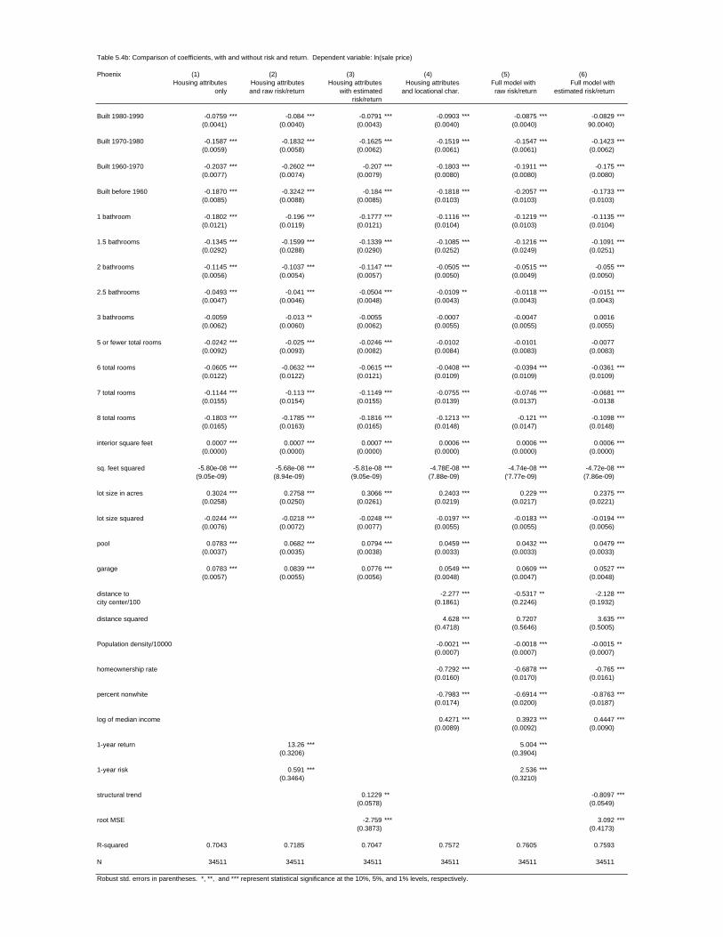
Table 5.4b: Comparison of coefficients, with and without risk and return. Dependent variable: ln(sale price)

Phoenix (1) (2) (3) (4) (5) (6)Housing attributes Housing attributes Housing attributes Housing attributes Full model with Full model with

only and raw risk/return with estimated and locational char. raw risk/return estimated risk/returnrisk/return

Built 1980-1990 -0.0759 *** -0.084 *** -0.0791 *** -0.0903 *** -0.0875 *** -0.0829 ***(0.0041) (0.0040) (0.0043) (0.0040) (0.0040) 90.0040)

Built 1970-1980 -0.1587 *** -0.1832 *** -0.1625 *** -0.1519 *** -0.1547 *** -0.1423 ***(0.0059) (0.0058) (0.0062) (0.0061) (0.0061) (0.0062)

Built 1960-1970 -0.2037 *** -0.2602 *** -0.207 *** -0.1803 *** -0.1911 *** -0.175 ***(0.0077) (0.0074) (0.0079) (0.0080) (0.0080) (0.0080)

Built before 1960 -0.1870 *** -0.3242 *** -0.184 *** -0.1818 *** -0.2057 *** -0.1733 ***(0.0085) (0.0088) (0.0085) (0.0103) (0.0103) (0.0103)

1 bathroom -0.1802 *** -0.196 *** -0.1777 *** -0.1116 *** -0.1219 *** -0.1135 ***(0.0121) (0.0119) (0.0121) (0.0104) (0.0103) (0.0104)

1.5 bathrooms -0.1345 *** -0.1599 *** -0.1339 *** -0.1085 *** -0.1216 *** -0.1091 ***(0.0292) (0.0288) (0.0290) (0.0252) (0.0249) (0.0251)

2 bathrooms -0.1145 *** -0.1037 *** -0.1147 *** -0.0505 *** -0.0515 *** -0.055 ***(0.0056) (0.0054) (0.0057) (0.0050) (0.0049) (0.0050)

2.5 bathrooms -0.0493 *** -0.041 *** -0.0504 *** -0.0109 ** -0.0118 *** -0.0151 ***(0.0047) (0.0046) (0.0048) (0.0043) (0.0043) (0.0043)

3 bathrooms -0.0059 -0.013 ** -0.0055 -0.0007 -0.0047 0.0016(0.0062) (0.0060) (0.0062) (0.0055) (0.0055) (0.0055)

5 or fewer total rooms -0.0242 *** -0.025 *** -0.0246 *** -0.0102 -0.0101 -0.0077(0.0092) (0.0093) (0.0082) (0.0084) (0.0083) (0.0083)

6 total rooms -0.0605 *** -0.0632 *** -0.0615 *** -0.0408 *** -0.0394 *** -0.0361 ***(0.0122) (0.0122) (0.0121) (0.0109) (0.0109) (0.0109)

7 total rooms -0.1144 *** -0.113 *** -0.1149 *** -0.0755 *** -0.0746 *** -0.0681 ***(0.0155) (0.0154) (0.0155) (0.0139) (0.0137) -0.0138

8 total rooms -0.1803 *** -0.1785 *** -0.1816 *** -0.1213 *** -0.121 *** -0.1098 ***(0.0165) (0.0163) (0.0165) (0.0148) (0.0147) (0.0148)

interior square feet 0.0007 *** 0.0007 *** 0.0007 *** 0.0006 *** 0.0006 *** 0.0006 ***(0.0000) (0.0000) (0.0000) (0.0000) (0.0000) (0.0000)

sq. feet squared -5.80e-08 *** -5.68e-08 *** -5.81e-08 *** -4.78E-08 *** -4.74e-08 *** -4.72e-08 ***(9.05e-09) (8.94e-09) (9.05e-09) (7.88e-09) ('7.77e-09) (7.86e-09)

lot size in acres 0.3024 *** 0.2758 *** 0.3066 *** 0.2403 *** 0.229 *** 0.2375 ***(0.0258) (0.0250) (0.0261) (0.0219) (0.0217) (0.0221)

lot size squared -0.0244 *** -0.0218 *** -0.0248 *** -0.0197 *** -0.0183 *** -0.0194 ***(0.0076) (0.0072) (0.0077) (0.0055) (0.0055) (0.0056)

pool 0.0783 *** 0.0682 *** 0.0794 *** 0.0459 *** 0.0432 *** 0.0479 ***(0.0037) (0.0035) (0.0038) (0.0033) (0.0033) (0.0033)

garage 0.0783 *** 0.0839 *** 0.0776 *** 0.0549 *** 0.0609 *** 0.0527 ***(0.0057) (0.0055) (0.0056) (0.0048) (0.0047) (0.0048)

distance to -2.277 *** -0.5317 ** -2.128 ***city center/100 (0.1861) (0.2246) (0.1932)

distance squared 4.628 *** 0.7207 3.635 ***(0.4718) (0.5646) (0.5005)

Population density/10000 -0.0021 *** -0.0018 *** -0.0015 **(0.0007) (0.0007) (0.0007)

homeownership rate -0.7292 *** -0.6878 *** -0.765 ***(0.0160) (0.0170) (0.0161)

percent nonwhite -0.7983 *** -0.6914 *** -0.8763 ***(0.0174) (0.0200) (0.0187)

log of median income 0.4271 *** 0.3923 *** 0.4447 ***(0.0089) (0.0092) (0.0090)

1-year return 13.26 *** 5.004 ***(0.3206) (0.3904)

1-year risk 0.591 *** 2.536 ***(0.3464) (0.3210)

structural trend 0.1229 ** -0.8097 ***(0.0578) (0.0549)

root MSE -2.759 *** 3.092 ***(0.3873) (0.4173)

R-squared 0.7043 0.7185 0.7047 0.7572 0.7605 0.7593

N 34511 34511 34511 34511 34511 34511

Robust std. errors in parentheses. *, **, and *** represent statistical significance at the 10%, 5%, and 1% levels, respectively.

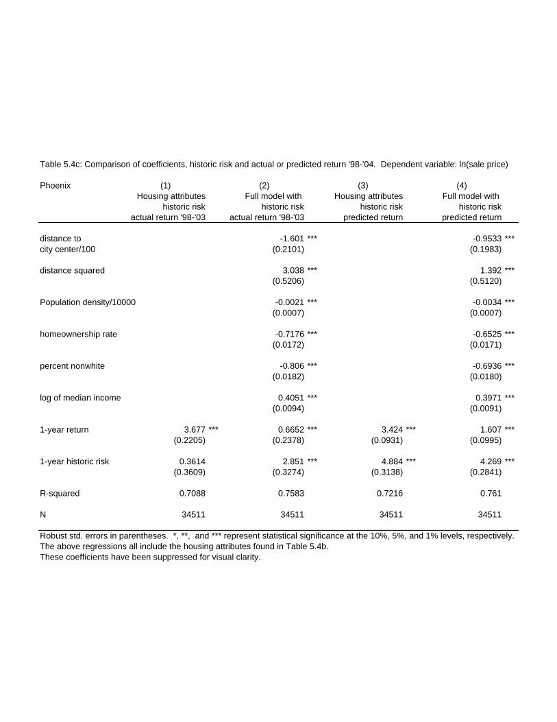
Table 5.4c: Comparison of coefficients, historic risk and actual or predicted return '98-'04. Dependent variable: ln(sale price)

Phoenix (1) (2) (3) (4)Housing attributes Full model with Housing attributes Full model with

historic risk historic risk historic risk historic riskactual return '98-'03 actual return '98-'03 predicted return predicted return

distance to -1.601 *** -0.9533 ***city center/100 (0.2101) (0.1983)

distance squared 3.038 *** 1.392 ***(0.5206) (0.5120)

Population density/10000 -0.0021 *** -0.0034 ***(0.0007) (0.0007)

homeownership rate -0.7176 *** -0.6525 ***(0.0172) (0.0171)

percent nonwhite -0.806 *** -0.6936 ***(0.0182) (0.0180)

log of median income 0.4051 *** 0.3971 ***(0.0094) (0.0091)

1-year return 3.677 *** 0.6652 *** 3.424 *** 1.607 ***(0.2205) (0.2378) (0.0931) (0.0995)

1-year historic risk 0.3614 2.851 *** 4.884 *** 4.269 ***(0.3609) (0.3274) (0.3138) (0.2841)

R-squared 0.7088 0.7583 0.7216 0.761

N 34511 34511 34511 34511

Robust std. errors in parentheses. *, **, and *** represent statistical significance at the 10%, 5%, and 1% levels, respectively.The above regressions all include the housing attributes found in Table 5.4b. These coefficients have been suppressed for visual clarity.

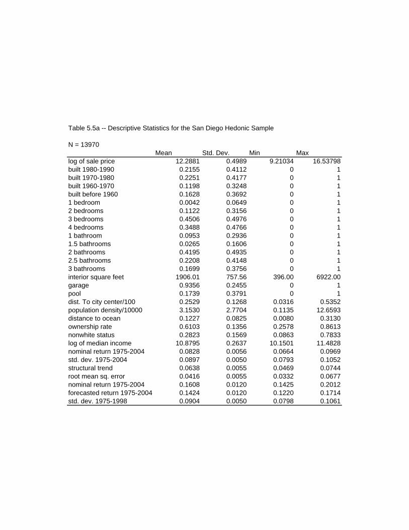
Table 5.5a -- Descriptive Statistics for the San Diego Hedonic Sample

N = 13970Mean Std. Dev. Min Max

log of sale price 12.2881 0.4989 9.21034 16.53798built 1980-1990 0.2155 0.4112 0 1built 1970-1980 0.2251 0.4177 0 1built 1960-1970 0.1198 0.3248 0 1built before 1960 0.1628 0.3692 0 11 bedroom 0.0042 0.0649 0 12 bedrooms 0.1122 0.3156 0 13 bedrooms 0.4506 0.4976 0 14 bedrooms 0.3488 0.4766 0 11 bathroom 0.0953 0.2936 0 11.5 bathrooms 0.0265 0.1606 0 12 bathrooms 0.4195 0.4935 0 12.5 bathrooms 0.2208 0.4148 0 13 bathrooms 0.1699 0.3756 0 1interior square feet 1906.01 757.56 396.00 6922.00garage 0.9356 0.2455 0 1pool 0.1739 0.3791 0 1dist. To city center/100 0.2529 0.1268 0.0316 0.5352population density/10000 3.1530 2.7704 0.1135 12.6593distance to ocean 0.1227 0.0825 0.0080 0.3130ownership rate 0.6103 0.1356 0.2578 0.8613nonwhite status 0.2823 0.1569 0.0863 0.7833log of median income 10.8795 0.2637 10.1501 11.4828nominal return 1975-2004 0.0828 0.0056 0.0664 0.0969std. dev. 1975-2004 0.0897 0.0050 0.0793 0.1052structural trend 0.0638 0.0055 0.0469 0.0744root mean sq. error 0.0416 0.0055 0.0332 0.0677nominal return 1975-2004 0.1608 0.0120 0.1425 0.2012forecasted return 1975-2004 0.1424 0.0120 0.1220 0.1714std. dev. 1975-1998 0.0904 0.0050 0.0798 0.1061

Table 5.5b: Comparison of coefficients, with and without risk and return. Dependent variable: ln(sale price)

San Diego (1) (2) (3) (4) (5) (6)Housing attributes Housing attributes Housing attributes Housing attributes Full model with Full model with

only and raw risk/return with estimated and locational char. raw risk/return estimated risk/returnrisk/return

Built 1980-1990 -0.0111 -0.0211 *** -0.0262 *** -0.0271 *** -0.0249 *** -0.0285 ***(0.0083) (0.0080) (0.0080) (0.0075) (0.0075) (0.0075)

Built 1970-1980 -0.0431 *** -0.0685 *** -0.0772 *** -0.0984 *** -0.0955 *** -0.1021 ***(0.0094) (0.0090) (0.0090) (0.0083) (0.0083) (0.0083)

Built 1960-1970 -0.0254 ** -0.0694 *** -0.089 *** -0.0825 *** -0.0784 *** -0.0797 ***(0.0113) (0.0109) (0.0111) (0.0102) (0.0103) (0.0102)

Built before 1960 0.0467 *** -0.0241 * -0.0672 *** -0.0522 *** -0.0508 *** -0.0549 ***(0.0132) (0.0124) (0.0133) (0.0127) (0.0127) (0.0127)

1 bedroom 0.1706 *** 0.3067 *** 0.2862 *** 0.1504 *** 0.1424 *** 0.1384 ***(0.0581) (0.0619) (0.0627) (0.0496) (0.0501) (0.0498)

2 bedrooms 0.1014 *** 0.1764 *** 0.16 *** 0.0971 *** 0.0881 *** 0.0886 ***(0.0182) (0.0178) (0.0180) (0.016) (0.0159) (0.0159)

3 bedrooms 0.0621 *** 0.1127 *** 0.1067 *** 0.0774 *** 0.0758 *** 0.0785 ***(0.0138) (0.0134) (0.0135) (0.0121) (0.0120) (0.0120)

4 bedrooms 0.0393 *** 0.0582 *** 0.0554 *** 0.0501 *** 0.0493 *** 0.0508 ***(0.0123) (0.0118) (0.0119) (0.0106) (0.0106) (0.0106)

1 bathroom -0.1896 *** -0.1415 *** -0.1484 *** -0.1074 *** -0.1116 *** -0.1086 ***(0.0286) (0.0273) (0.0273) (0.0246) (0.0246) (0.0245)

1.5 bathrooms -0.1883 *** -0.1263 *** -0.1300 *** -0.0755 *** -0.0812 *** -0.0790 ***(0.0313) (0.0301) (0.0301) (0.0269) (0.0268) (0.0268)

2 bathrooms -0.0993 *** -0.0511 ** -0.0544 ** -0.0296 -0.0275 -0.0271(0.0235) (0.0222) (0.0223) (0.0203) (0.0202) (0.0202)

2.5 bathrooms -0.0826 *** -0.0636 *** -0.0659 *** -0.054 *** -0.0515 *** -0.0507 ***(0.0216) (0.0202) (0.0203) (0.0187) (0.0186) (0.0186)

3 bathrooms -0.0702 *** -0.0497 *** -0.0512 *** -0.0447 ** -0.0443 ** -0.0444 **(0.0200) (0.0187) (0.0188) (0.0173) (0.0173) (0.0172)

interior square feet 0.0007 *** 0.0007 *** 0.0007 *** 0.0005 *** 0.0005 *** 0.0005 ***(0.0000) (0.0000) (0.0000) (0.0000) (0.0000) (0.0000)

sq. feet squared -4.45e-08 *** -5.60e-08 *** -5.36e-08 *** -3.26e-08 *** -3.17e-08 *** -3.11e-08 ***(4.93e-09) (4.82e-09) (4.85e-09) (4.49e-09) ('4.50e-09) ('4.47e-09)

pool 0.0401 *** 0.0477 *** 0.1355 *** 0.0549 *** 0.056 *** 0.0569 ***(0.0086) (0.0082) (0.0082) (0.0076) (0.0076) (0.0076)

garage 0.1469 *** 0.1349 *** 0.049 *** 0.1149 *** 0.1114 *** 0.1121 ***(0.0145) (0.0140) (0.0140) (0.0124) (0.0123) (0.0123)

distance to -1.142 *** -0.9582 *** -0.5148 ***city center/100 (0.1343) (0.1393) (0.1393)

distance squared 1.362 *** 0.4539 0.3359(0.2353) (0.2803) (0.2803)

Population density/10000 0.0003 -0.0071 *** -0.0053 ***(0.0015) (0.0017) (0.0015)

distance to ocean/100 -0.6137 *** -0.5954 *** -0.5213 ***(0.1521) (0.1633) (0.1675)

distance to ocean -0.0052 0.2651 0.1774squared (0.5034) (0.4995) (0.5063)

homeownership rate -0.8904 *** -0.7324 *** -0.776 ***(0.0343) (0.0367) (0.0352)

percent nonwhite -0.6621 *** -0.7103 *** -0.5492 ***(0.0198) (0.0209) (0.0223)

log of median income 0.6371 *** 0.6111 *** 0.6592 ***(0.0203) (0.0201) (0.0213)

1-year return 17.67 *** -2.660 **(1.371) (1.325)

1-year risk -3.770 *** 11.01 ***(1.122) (1.158)

structural trend 15.77 *** 1.769(0.6021) (1.388)

root MSE 6.209 *** 8.995 ***(0.6729) (0.7776)

R-squared 0.5370 0.5703 0.5697 0.6546 0.6750 0.6576

N 13970 13970 13970 13970 13970 13970

Robust std. errors in parentheses. *, **, and *** represent statistical significance at the 10%, 5%, and 1% levels, respectively.

Table 5.5c: Comparison of coefficients, historic risk and actual or predicted return '98-'04. Dependent variable: ln(sale price)

Phoenix (1) (2) (3) (4)Housing attributes Full model with Housing attributes Full model with

historic risk historic risk historic risk historic riskactual return '98-'03 actual return '98-'03 predicted return predicted return

distance to -1.470 *** -0.9596 ***city center/100 (0.1469) (0.1397)

distance squared 1.274 *** 0.5788 **(0.2585) (0.2584)

Population density/10000 -0.0057 *** -0.0075 ***(0.0017) (0.0017)

distance to ocean/100 -0.6565 *** -0.5209 ***(0.1505) (0.1511)

distance to ocean 0.4049 0.1904squared (0.4977) (0.4987)

homeownership rate -0.6497 *** -0.7526 ***(0.0385) (0.0392)

percent nonwhite -0.6369 *** -0.6836 ***(0.0201 (0.0221)

log of median income 0.4843 *** 0.6335 ***(0.0259) (0.0238)

1-year real return -8.903 *** -4.682 *** 7.996 *** -0.7137 ***(0.3452) (0.5573) (0.2981) (0.3974)

1-year real risk 9.911 *** 11.68 *** 4.687 9.841 ***(0.7160) (1.117) (0.6301) (1.124)

R-squared 0.5612 0.6584 0.5617 0.6569

N 13970 13970 13970 13970

Robust std. errors in parentheses. *, **, and *** represent statistical significance at the 10%, 5%, and 1% levels, respectively.The above regressions all include the housing attributes found in Table 5.5b.These coefficients have been suppressed for visual clarity.