The issue of classification versus precision rates in …nymetro.chapter.informs.org/prac_cor_pubs/09-2015...Pred Non Pred Event Total Actual Non-event A A / E =TNR A / G = NPR B B

10/5/15 Leonardo Auslender Copyright 201510/5/15 1

The issue of classification versus precision rates in comparing classification models

Informs NYC 2015/09.

By Leonardo Auslender

Independent Statistical Consultant Leonardo.Auslender ‘at’ gmail ‘dot’ com


Setting and topics of discussion.

Binary Target Models, used in DM, Finance, Telco, Clinical, etc.

Target variable usually denoted by Y and accepts two values or labels, “0” (non-event) and “1” (event). Typically, proportion of events << proportion of non-events.

Predictions are usually classified as “events” (“1”) whenever posterior probability > cutoff. Else, non-event (“0”). “Known” cutoff value assumed in this section. Tree models use an implicit cutoff point, usually .5.

Goals: Model Comparison.

Decision on model deployment.

Model(s) outcome easily portrayed in 2 x 2 table, called Classification or Confusion Table.

2 sets of examples: 1st based on 3 models of Titanic survivors. Each model differs in variables utilized for prediction and 2nd two fraud models.

Model details not shown for brevity. No K-S or other measures discussed much.



Pred Non Pred Event Total ActualNon-event A (TN): true

negativeB (FP): false positive

A + B

Event C (FN): false negative

D (TP): true positive

C + D

Total Predicted

A + C B + D A + B + C + D = Grand Total

Classification (Accuracy) Rate: 100 (A + D) / grand total. Positive Precision Rate: PPR = 100 * D / B + D. Sensitivity = Event class-recall- (hit) rate = TPR = 100 * D / C + D Specificity = Non-Event classification rate TNR = 100 * A / A + B.1 – Specificity = Event miscl. rate (false alarm) FPR = 100 * B / A + B. F1-measure = 2 / [ (1 / precision) + (1 / recall)] (geom. Mean of prec. & recall), (Van Rijsbergen, 1979).

Mutual Information =

Classification (confusion) Table (similar tables and analysis for other than 2 * 2).

2 2

1 1

( , )( , ) log

( ) ( )t p

t pt p t p

P Y XP Y X

P Y P X= =∑∑


Classification rate

Proportion of events predicted as events (similarly for non-events). (Also called recall or True Positive Rate (TPR). When considering events and non-events together, called accuracy or overall classification rate of events and non-events).

Denominator is number of original events and non-events, which is fixed for any original ratio of events and non-events (ratio called prior, skew, etc). Thus, in previous slide, TPR = 100 * D / (C + D).

Demsar (2006) shows most algorithms compared based on accuracy.

Precision Rate:

Proportion of predicted non-events/events that are truly non-events/events. Thus, PPR = 100 * D / (B + D).

Denominator is number of predicted events and non-events, which is conditional on any prior number of events.

Pred Non Pred Event Total Actual

Non-event A A / E =TNR A / G = NPR

B B / E = FPR E

Event C C / F = FNR D D / F = TPR D / H = PPR

F

Total Predicted G H I


Graphical Appreciation.

FP

∩= = =

+

∩= = =

+

| Predicted_Events Event |Pos.Precision

| Predicted_Event |

| Predicted_Event Event |Pos.Classif

| Event |

TPPPR

TP FP

TPTPR

TP FN

Non-Events

Predicted Events: everywhere else outside of oval, is predicted non-events.

FN

TPEvents


Example of Accuracy vs. Precision. Hand (2007, pp. 22-23), fraud study, classifier:

Correctly identifies 99 in 100 legitimate transactions è TNR = 99%Correctly identifies 99 in 100 fraudulent transactions è TPR = 99%

Assume 1 in 1000 is fraud (prior = prevalence = .001).

Pred Legit Pred Fraud Total ActualLegit 99% /

989.011% / 9.99 100% / 999

Fraud 1% / 0.01 99% / 0.99 100% / 1

Total Predicted

100% / 989.02

100% / 10.98 100% / 1000

Fraud Precision rate: 0.99 * 100 / 10.98 = 9.016% è 90% predicted frauds are legitimate transactions. Legit Precision Rate = 989.01 * 100 / (989.01 + 0.01) = 99.9%, almost all predicted legits are legits.


On what information should we focus?

TPR = Pr ( Pred (Y) = 1 / Y = 1)

PPR = Pr (Y = 1 / Pred (Y) = 1)

Or the square root of the sum divided by ‘e’?

10/5/15 Leonardo Auslender Copyright 201510/5/15

Example of Bayesian modeling (Ayres (2007), p. 213-214).

Pr (breast cancer at 40) = Prior = 1%.Pr (Positive diagnosis / Cancer) = TPR = 80%.Pr (Positive diagnosis / no cancer) = FPR = 10%.40 year old woman had positive diagnosis.

Q.: Pr (Cancer / positive diagnosis)? 80%?, 8% (TPR * PRIOR)?, some fudge of TPR and FPR? (note that TPR + FPR ≠ 100%).

Pred Healthy Pred Cancer Total Actual

Healthy 90% / 891 10% / 99 (FPR) 99% / 990

Cancer 20% / 2 80% / 8 (TPR) 1% / 10

Total Predicted 100% / 893 100% / 107 100%/ 1000


++ = =+ + +

=

= =+

=

Bayes Theorem:

Pr( ) *Pr( / )Pr( / )Pr( ) *Pr( / ) Pr( ) *Pr( / )

Prior*TPRPrior*TPR+(1-Prior)*FPR

.01*.80.01*.80 .99 *.10

.075 8 /107.

C CCC C C C

Detour: Bayes Theorem:

Note that in order to find Pr (C/+), the only necessary information is TPR and FPRthat originate from the ‘predicted’ column only.

In Business environment, Pr (C/ +) == Pr (Fraud / predicted fraud) == Pr ( Responder/ predicted responder). Pr ( C ) = .01 is no longer relevant for the patient. TPR and FPR‘known’ from previous work and chosen cutoff.


Bayesian Formula and Modeling.

Bayes’ formula updates original unconditional probability of cancer 1% with the new information from test diagnostic.

Probability jumps from 1% to 7.5% è

1) Modeling by “conditioning” on test diagnostic è update of information.

2) Notice that Bayes’ result is ‘our’ measure of precision è once Test diagnostic (model) is available, unconditional probability (PRIOR), TPR, FNR irrelevant (if you believe in given test). PPR and NPR become relevant.

12


Neglecting Costs and Getting a Cost headache.

If misclassification costs were equal (FNR and FPR costs), then could replace FNR and FPR by overall misclassification measures.

But, cost of classifying as Legit when is actually fraud case VERY DIFFERENT from classifying as fraud when legit.

If classify as Legit when it is a fraud case, business incurs direct loss.

If classify as fraud when legit, business does not directly incur loss but may lose customers due to loss of customer good-will.

Modeler may decide to minimize loss function, or better, maximize profit function, which requires FNR and FPR costs:

π ππ

π π

= += = =

= − + −iPrior Prob (Y=i), c miscl. cost into i, r ith revenue.

Profit ( ) ( )i i

Loss c FNR c FPR

r TNR c FNR rTPR c FPR

0 0 1 1

0 0 0 1 1 1


More terminology, just to summarize. Conditional probabilities.

TPR = Prob ( PRED POS / POSITIVE (EVENT)) = TP / (TP + FN) = Cum % captured events (DM).

TNR = Prob (PRED NEG / NEGATIVE (NO EVENT)) = Correct Rejection

FPR = Prob (PRED POS / NEGATIVE (NO EVENT)) = 1 – TNR = False Alarm = Type I error

FNR = Prob (PRED NEG / POSITIVE (EVENT)) = Miss = Type II error

PPR = Positive Precision rate = Purity = Prob ( POS / PRED POS)) = TP / (TP + FP) = Cum % events (and from this, lift, etc in DM).

NPR = Negative Precision Rate = P (NEG / PRED (NEG)) = TN/ (TN + FN)

Unconditional Probabilities.

Prevalence = risk = P (Positive) Used mostly in clinical studies.


Classification table as goodness-of-fit?

1.  Good model may classify poorly: Hosmer and Lemeshow (2000, p. 157): model with expected misclassification rate dependent on coefficient slope, not on model fit of logistic regression (unsystematic distances between observed and predicted).

2.  Classification done by choosing cutoff point in posterior probability. Well known that classification favors majority group, which is independent of model fit. Thus, if P1 = .49 and P2 = .52, and cutoff is .5, observations classified into different categories when probabilities very close.

Assumes known and unchanging “natural” class distribution and that error cost of FP = errors FN. Typically favors majority class; but in most applications, cost of misclassifying “1” is higher.


Accuracy can mislead, comparing 2 models (right and left). Example 1: Assume “1” important. Left Overall Accuracy = 92.5%,

Right overall accuracy = 97.5%, but right model misses all “1”s.

Example 2: 80% accuracy in two models. If test data set contains more “0”s, right model better. If more “1”s, left model.

Accuracy=92.5%

Predicted 0 Predicted 1 Accuracy=97.6%

Predicted 0 Predicted 1

Actual 0 180 15 195 0Actual 1 0 5 5 0

Precision 100% 25% 97.5% ?

80% acc. Predicted 0 Predicted 1 80% acc. Predicted 0 Predicted 1Actual 0 40 10 50 0Actual 1 10 40 20 30Precision 80% 80% 71% 100%

è


Classification table as goodness-of-fit?

3. Models from different samples cannot be compared based on these tables because predicted probabilities are confounded by the distribution of probabilities in original samples.

4. Classification error may increase when highly significant variable (however defined) is added to model. Classification error is insensitive and inefficient measure. Use Brier’s instead (Pencina et al, 2008). Some authors (Provost et al (1998) prefer ROC, while others (Harrell) used to prefer ROC and switched to Brier (to be discussed in the future).

− −=ˆ ˆ(Y Y)'(Y Y) ˆBrier , Y : posteriorN



Classification Costs Specific by Industry and discipline.

Pred non-resp

Pred resp

Non-resp TN FP

Resp. FN TP

DMers: FNR more important than FPR because FN are not targeted and lose potential revenue of fees & purchases on lifetime basis. Cost of reaching FP usually disregarded è DMers should concentrate on minimizing FN errors. Since FNR = 1 – TPR, equivalent to maximizing TPR, Let's denote (reviewed later) shows higher point of TPR. Max Likel minimizes FP + FN usually.

In fraud case, minimizing FNR may still leave bad “precision” for fraud cases.


Classification Costs Specific by Industry and discipline.

Suppose QC of toy screw manufacturing, positive = defective. FP may induce costly retooling, FN depends on toy and intended age, often disregarded. If screw is instead critical part of bridge which could fall, FN obviously costlier.

In Information Retrieval (e.g., web search) TPR not so important because if retrieve 5,000 references, ranking of references of top 50 or so more important than overall TPR è Lift (next section).

In Clinical and marketing analyses, event rates can be very low (called prevalence in clinical, or priors). In this case a test may yield high FP rates that are higher than the FN rates.

In this case a small PPR rate yields high FPR even if the TNR is close to 100%.


Are False positives less Important?

Database Technologies (DBT) was hired by Florida to create list of potential people to remove from list of voters (Ayres, 2007, p.137).

DBT matched registered voters to national lists of felons and was required 90% match between voters’ and felons’ names, (rough) birthday and race è many false positives emerged è 57,746 registered voters identified as convicted felons. (felon = positive).

Since higher proportion of convicted felons are black, higher proportion of black people were false positives than whites.

Clearly, not possible to request 100% matching. And no False Negative study ever done.

Highly debatable issue in civil rights.



Changing % of Non-events and Events per prob. cutoff


ROC and LIFT

Let's denote posterior probability or any monotonic transformation thereof as S (Y). Thus, for given s in [0, 1], TPR = Pr (S > s / Y = 1). And likewise, PPR = Pr (S > s / Pred (Y) = 1). S and s in [0, 1] and typically s = [0, .1, .2,,,,,,,, 1].

Receiver Operating Characteristics (ROC) curve graphs or tabulatespairs of TPR (in the y-axis) and FPR (1 – specificity, in the x-axis) fordifferent levels of s in S. That is, TPR(s) vs. FPR (s).

Lift graphs or tabulates TP (s) vs. Pr (S > s) (note: PRECISION based measure), and gains chart tables provide information on cumulative percentage of captured responders and of true events at point s. Lift measure is usually divided by the overall response rate, i.e., by TPR (s = 0). Lift tables usually presented as part of Gains Tables.

Note that neither ROC nor LIFT recommends cutoff point straightforwardly.


ROC and Cutoff Probabilities.

ROC building based on simulating probability cutoff changes from 0 to 1 (s). Can imagine series of classification tables for varying probability cutoffs and collecting TPR and FPR. Below, two tables for cutoff = 25% and 75% for models 1 through 3.

Class. Table

Predicted as

Non-Event

Event

Value Value

Study # Event Non-Event Status

0.84 0.16

1 Non-Event

Event 0.31 0.69

2 Non-Event 0.63 0.37

Event 0.13 0.87

3 Non-Event 0.65 0.35

Event 0.17 0.83

Class. Table

Predicted as

Non-Event

Event

Value Value

Study # Event Non-Event Status

0.88 0.12

1 Non-Event

Event 0.60 0.40

2 Non-Event 0.96 0.04

Event 0.51 0.49

3 Non-Event 0.97 0.03

Event 0.45 0.55


Different priors, Same AUROC, Different Accuracy, cutoff andPrecision.


A

BC

ROC model selection. Curves can cross. NW direction è better model. B is preferred to C for low FP rates, but C preferred over B later on. A clearly inferior.

“Best” model: max AUROC (area under curve and above 45* line). But max AUROC may not be ‘best’ for specific cost and class distribution.


Area under curve (AUROC or “c” statistic) shows % of pairs of (0 / 1) such that predicted probability for “1” > predicted probability “0” (same as Mann-Whitney U statistic (Bamber, 1975)) or Wilcoxon test of ranks.

(Also, related to Gini = Sommer’s D = 2 AUROC – 1.)

For randomly chosen event / non-event pair, AUROC = Prob (Event > Non-Event).

AUROC can be considered as the average TPR across all possible FPR.


ROC, Lift and Data priors.

ROC unaffected by different data priors or cost distributions (except when target variable was created by dichotomizing from continuous variable and probable measurement error, likely in clinical studies (Brenner, Gefeller, 1997)).

Note that ROC (and AUROC and KS) depend on probability ranking that does not change with priors. Precision, lift, F-score are affected by changes in priors.

è Same algorithm applied on 2 test data sets with different class balances but same number of events show same ROC curves, but precision-recall (recall = TPR) curve changes.

REMARK: Since cutoff (and model) can be chosen based on Precision and TPR, can use Precision-Recall curve to combine them that is affected by different priors (presented below).


Gains Table / Chart generation.

1)  Table in descending order of cutoff probability, usually shown in deciles (10%), demi-deciles (5%) or vingtiles (20%) intervals of counts of observations.

2)  Events expected to bundle at top of table for ‘good’ model.

3)  Obtain PPR and derivations thereof, such as lift and cumulatives. (% true events, %captured all events).

4) Interpretation: search for cutoff “decile” (or percentile, etc) based on criterion (profit, specific cumulative response rate, etc.), and consider as “events” observations above cutoff. Note: percentages and counts are of actual observations, not predicted, since posterior probability is used as index in decile creation.


Gains Table measures.“Cumulative” accumulate from top of probability to bottom in similar fashion as ROC from left to right.

Cum % events = Event Precision. If 1st decile is contacted/targeted, equivalent to predicting all observations as events è Cum % events in decile = precision è lift and gain are mere transformations of precision as well è

If cutoff (and sometimes model itself) chosen based on Lift, cutoff (and model) actually based on PRECISION (which is not part of ROC).

Lift: % Events in decile / Prior % events in pop, and corresponding cumulative.

Gain: (% events in decile / Random % events in decile ) – 1 (not very used).

Cum % captured events = True positive Rate (belongs in ROC). As cutoff is shifted down the table, Cum % captured = proportion predicted events that are truly events è if cutoff (and model) based on TPR achieved at specific percentile è cutoff (and model) chosen based on classification measure.


Gains Table Events Rate

Cum Events Rate

% Event Captured

Cum % Events

Captured Lift Cum Lift Brier Score *

100

Percentile Model Name

63.087 63.087 31.623 31.623 3.162 3.162 21.374 10 LOGISTIC_STEPWISE

TREES 71.708 71.708 35.945 35.945 3.594 3.594 0.000

20 LOGISTIC_STEPWISE 34.899 48.993 17.494 49.117 1.749 2.456 22.474

TREES 30.658 51.183 15.367 51.312 1.537 2.566 0.000

30 LOGISTIC_STEPWISE 21.141 39.709 10.597 59.714 1.060 1.990 16.726 TREES 23.467 41.944 11.763 63.075 1.176 2.103 0.000

40 LOGISTIC_STEPWISE 18.960 34.522 9.504 69.218 0.950 1.730 15.362 TREES 19.920 36.438 9.985 73.060 0.999 1.827 0.000

50 LOGISTIC_STEPWISE 13.591 30.336 6.812 76.030 0.681 1.521 11.817

Gains Table Example comparing 2 models.(Brier score not yet computed for Trees)


100

120

140

160

180

200

220

240

100


Single misclassified obs causes this drop.


Precision – Recall Curves.

Many situations in which priors and costs are unknown. Could also be case in which priors and costs actually vary, either in time or by subpopulations. E.g., prevalence of certain diseases differs across races or ethnic groups but the individual cannot be properly identified. Certainly prevalence of diseases and other events changes with time. E.g., obesity rates in the US in the past 30 years.

In these cases, ROC and threshold cutoff not so reliable because ROC does not reflect changes in priors.



0.43

Compromise?: Cutoff: intersection precision curve and TPR: no theory behind.


239

80

Cutoff point selected at top 80th percentile of prob. Distribution.

Money Matters: Profits determine cutoff.


ROC components and KS to determine cutoff point. Highest separation point.

Plot sensitivity and specificity (Y) vs. prob. cutoff points (X). Intersection indicates maximum separation (K-S test). No cost specified.


Using ROC with financial information to determine cutoff via ROC - Direct Marketing Application.

Suppose mailing data base 10,000 candidates. Expect 10% response rate è if mail everybody, expect 1,000 responders. Assume budget constraint that allows to mail to just 3,500 è

FPR * 9,000 + TPR * 1000 = 3,500, orTPR = 3.5 – FPR * 9

From ROC graph, locate pair (FPR, TPR) that satisfies equation, derive cutoff point and contact those above cutoff point.

But this is wrong because TPR + FPR ne 100%. Instead, use PPR and (1 – PPR).


ModelsComparison.



Note on ROC Comparisons.

Without looking at AUROC, Models 2 and 3 are preferable to 1. But Model 3 has a far shorter range of pairs of TPR and FPR than model 2.

For specific FNR, underlying cutoff points for each models are different (.35, .42, .22 respectively, from left to right). Implicitly, ROC curves have 3rd axis not shown of descending probability è choosing model based on ROC implies specific cutoff for THAT model cannot necessarily be used for another model, either for implementation or to compare classification tables.

There is no single measure or way to select ‘the’ model. A complex model that validates well may not be so robust to changing business/other conditions as simpler and ‘not so good’ model.


Model 2

Model 3

AUROC2 > AUROC3, but ‘3’ has larger % non-events in lowest grouping.

Model 2

Model 3

Non-events higher probability than events è AUROC < 1.


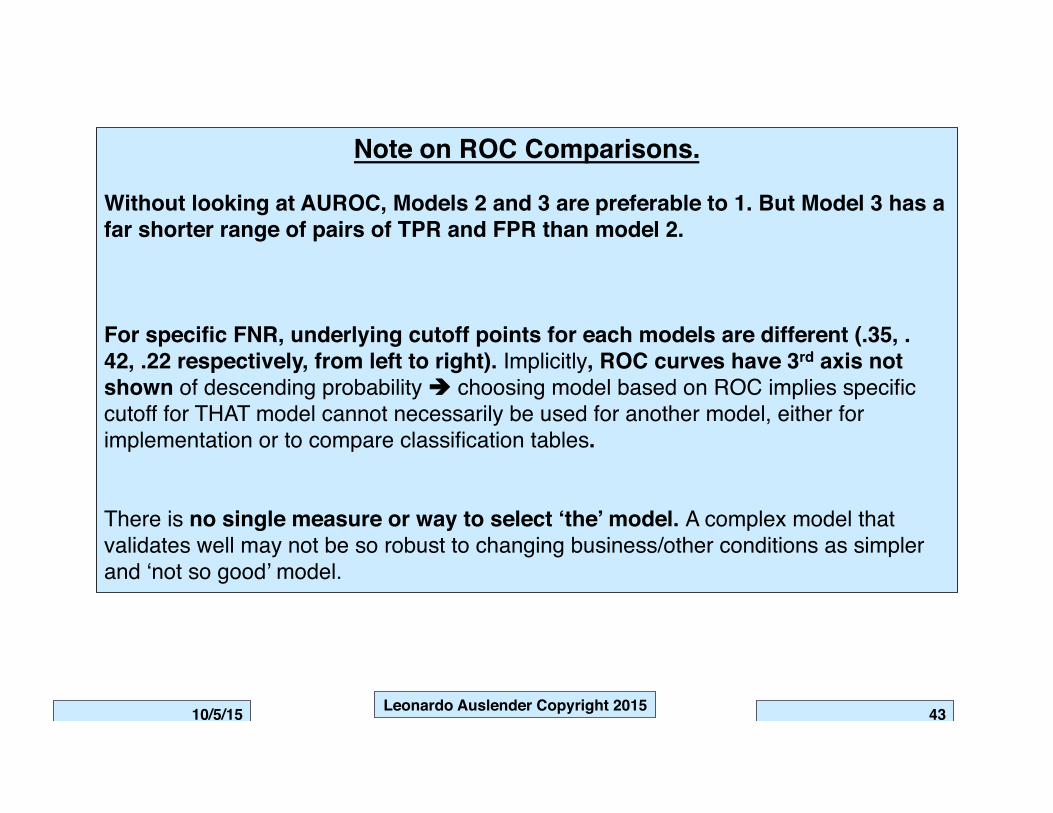
Model 3 finds higher proportion of events and non-events in extremes of score distribution. If interested in targeting very few positives, model 3 is preferable to model 2, despite fact that AUROC 2 > AUROC 3.

But also note that for non-extreme observations, model 3 is not a good discriminator.

K-S does not provide any useful information short of stating that the models differentiate and providing point of maximum difference. Note that those points are not necessarily optimal as cutoffs.

Likewise, ROC per se does not provide any optimal cutoff point.


0

100

200

300

100


100


Cutoff set by maximum Cumulative Profit from gains table. If Model 2 selected, cutoff = 0.70.



Training: Rates '-' ==> misclass & Missprec

Predicted Class

0 1 Overall

Class Rate Prec Rate Class Rate Prec Rate Class Rate Prec Rate

Fraudulent Activity yes/no Model Name

97.30 83.73 -2.70 -31.01 97.30 0 LOGISTIC_STEPWISE

TREES 98.87 84.66 -1.13 -13.92 98.87

1 LOGISTIC_STEPWISE -75.86 -16.27 24.14 68.99 24.14

TREES -71.91 -15.34 28.09 86.08 28.09

Overall LOGISTIC_STEPWISE 83.73 68.99 82.70 82.70

TREES 84.66 86.08 84.75 84.75

Note that TPR is rather low while PPR is quite high (prevalence = 20%).





Conclusions:

1)  Precision contains information conditioned on the new information available, e.g., clinical test, demographics. It answers the question of probability of response/sick/survival given present information.

2)  Do classification and precision measures typically rank order well? Yes, but they don’t indicate good models necessarily.

3)  Are models results reliable by just these measures? NO. 4)  To-do list:

1) Residual analysis (Pardoe, many papers).2) Calibrate models.3) Average and/or take median of predictions as additional

model. 4) Inference on lift measures to determine whether model

results not very different (Jiang, forthcoming in JASA, Ratner (Web)).


Documents

The issue of classification versus precision rates in …nymetro.chapter.informs.org/prac_cor_pubs/09-2015...Pred Non Pred Event Total Actual Non-event A A / E =TNR A / G = NPR B B