1

The Italian educational system: family background and social stratification†

Daniele Checchi – University of Milan

final version: January 2003

Contents: 1. Introduction ........................................................................................................................................................ 2 2. Some comparative evidence.............................................................................................................................. 3 3. Potential explanations ........................................................................................................................................ 7

3.1 – Wrong expectations ................................................................................................................................. 7 3.2 – Low returns to education ...................................................................................................................... 10 3.3 – Limited (public) resources invested in education .............................................................................. 12

4. Additional evidence on family background .................................................................................................. 16 5. Concluding remarks ......................................................................................................................................... 24 References.............................................................................................................................................................. 27 Appendix................................................................................................................................................................ 29 Daniele Checchi Facoltà di Scienze Politiche Università degli Studi di Milano via Conservatorio 7 20122 MILANO - Italy tel. +39-02-503-21519(dir) 21501(secr) fax +39-02-503-21504 email daniele.checchi@unimi.it

† Paper presented for the ISAE conference on Monitoring Italy (10/1/2003). The author acknowledges many valuable comments from the participants. Many ideas presented in the papers originate form joint work with different co-authors, whom I would like to thank without implicating: Giuseppe Bertola, Giorgio Brunello, Valentino Dardanoni, Andrea Ichino, Tullio Jappelli and Francesco Zollino. Remaining errors are my own responsibility.

2

…what is now known about early childhood development. The essence of that knowledge is not complicated: learning begins at birth, and a loving, secure, stimulating environment, with time devoted to play, reading, talking and listening to infants and young children, lays down the foundations for cognitive and social skills. No government can therefore ignore the issue of what happens in the preschool years.

Unicef 2002, pg.3 1. Introduction Human capital accumulation is widely recognised as a crucial factor for economic and social policies in modern societies. Individual returns to schooling have been proved positive for almost all countries, both in terms of steeper age-earning profiles and improved employment probability (Blöndal, Field and Girouard 2002). Not only the average educational attainment in a country, but also its distribution in the population plays a role in explaining growth performance over recent decades, for both developed and developing countries (Lopez, Thomas and Wang 1998, Bassanini and Scarpetta 2001). Finally, increased access to education is typically correlated with improvement in health, reduction in fertility, longer life expectancy, decline in crime rates and increase in use of liberty rights (UNDP 2001). Even taking into account the full cost of education, typically financed on public funds, the social returns to education are higher than both real rates of interest and rates of return on other productive assets, thus indicating the convenience of further investment in education. When we look at participation rates, a common evidence from a number of countries suggests that the minority of young people who fail to complete upper-secondary education tend to come from less affluent backgrounds. In many Mediterranean countries, including Italy, universal participation in secondary school still remains a challenge for public authorities. If we go at tertiary education, the participation of young people is highly correlated with the educational attainment of their parents. Thus increasing school participation has a double-edged challenge: on the grounds of efficiency, by improving the average educational attainment, public authorities may hope to increase country’s productivity and competitiveness; on the equity ground, since students from better family backgrounds (both in terms of education and income) already achieve the highest levels of education, average educational attainment can only be achieved by mostly improving the participation of youngsters from poor social conditions. The present paper analyses the low educational attainment characterising Italy with respect to other countries, and explores potential causes of this phenomenon. Given the high intergenerational persistence, it focuses on the mechanism of education transmission, and finds that early tracking is strongly correlated with parental education. Once children are channelled into different tracks (technical/vocational secondary schools on one side, academic oriented high schools on the other), transition to university is heavily dependent on past schooling, but parental education still plays a role. On the contrary, family income seems not to prevent educational attainment, such that “cultural constraints” seems a more appropriate description of the problem of Italian tertiary education than “liquidity constraint”. Once we have assessed this evidence, it is not easy to put forward solutions to the problem. Nevertheless, given the scant evidence on the effect of school resources on children performance, our analysis points to put greater efforts to reduce parental influence on children’s schooling: early schooling; full day schooling instead of homework; adult participation in formal education; later tracking; reversibility of choice; and so on. The paper ignores other related aspects of educational attainment, the most important of which is the debate about over-education. Despite of the low participation in education, a significant share of employed labour force typically declare to possess inappropriate and/or excessive knowledge with

3

respect to the requirement of the job they take.1 While the debate on over-education in Italy dates back at least one century (Barbagli 1974), a formal analysis requires information on the demand for skills by enterprises, information that still is lacking in our country. Thus the paper depicts a supply side analysis of educational achievement (or failure) under the assumption of constant demand for human capital in the labour market. The paper is organised as follows. In section 2 we review existing empirical evidence over the lower educational attainment in Italy when compared to other major European countries. Our country is also characterised by low intergenerational mobility, even if recent cohorts face an improved situation. Section 3 discusses alternative explanations of this evidence, taking into account wrong expectations formation, low returns to education and low resources invested in education. These explanations are all disregarded for being unable to explain both low achievement and strong parental dependence. Section 4 provides new evidence on the intergenerational persistence in educational attainment, showing that family income is statistically irrelevant, whereas parental education matters in attending secondary school and university. However, most of the effect of parental education passes through the choice of secondary school (high school versus technical schools), a choice that in Italy is undertaken quite early (when the child is aged 13). Section 5 contains some concluding remarks and discuss some policy options. 2. Some comparative evidence By international standards, Italy is characterised by low educational attainment, even if most recent cohorts seem to catch up in order to reduce the gap. Looking at tables 1 (and A.1 in Appendix), one can notice that this gap is not reduced when taking into account the fact that labour market participation increases with the educational attainment: slightly less than half of the Italian population (slightly more than half when considering the labour force) in the relevant age goes beyond compulsory education.2 This is obviously the result of Italy being a country of late industrialisation and late mass scholarisation, as it can be grasped by comparing secondary educational attainment by age cohorts, as reported in table 2. By looking at the last row of this table, one can see that the educational gap from the average declines by 2-3 percentage points each decade. Should the speed of catching up remain similar in the nearby future, we could expect Italy to reach the average of OECD countries (but not the best performers) in 80 years, which appear a very long-term horizon.

1 With respect to the Italian case, Ghignoni 2001 estimates “competence frontiers” (obtained under the assumption that work experience substitutes for lack of formal education), finding that 70% of the labour force achieves education in excess over the one required by the job. However, Rossetti and Tanda 2001 follow a multidimensional approach to analyse the benefits of education (satisfaction, flexibility, autonomy), showing that agents may be interested in obtaining more education in order to increase their probabilities to obtain better jobs. 2 We cannot count as falling short compulsory education the population share reported in the first column, since lower secondary education was made compulsory in 1962, thus affecting all age cohorts born after 1952. In Checchi 1998 we have measured educational poverty as the population share not attaining the compulsory obligation legally relevant for their cohort, when the 60% was already accomplishing the obligation. This correction is made necessary by the fact that legal obligation is per se insufficient to yield people accomplishment: the Gentile reform had already introduced a formal obligation of 8 years of schooling in 1923, but it took up to the seventies to attain enrolment rates close to 100% (see Checchi 1997a). The estimated educational poverty was 10.2% in the entire population taken to census in 1991.

4

Table 1 – Educational attainment of the population aged 25-64 (2001)

Pre-primary and primary education

(ISCED 0/1)

lower secondary (ISCED 2)

short (3 yrs) upper

secondary (ISCED 3b-c)

long (5 yrs) upper

secondary (ISCED 3a)

tertiary type-B

education (ISCED 4)

tertiary type-A

education (ISCED 5/6)

France 18 18 31 10 11 12 Germany 2 16 52 3 15 13 Italy 22 33 8 25 2 10 Japan -- 17 -- 49 15 19 United Kingdom -- 17 42 15 8 18 United States 5 8 -- 50 9 28 OECD average 15 19 19 22 11 15

Source: OECD 2002a, table A3.1a

Table 2 – Population that has attained at least upper secondary education by age cohort (2001) 25-64 25-34 35-44 45-54 55-64 France 64 78 67 58 46 Germany 83 85 86 83 76 Italy 43 57 49 39 22 Japan 83 94 94 81 63 United Kingdom 63 68 65 61 55 United States 84 88 89 89 83 OECD average 64 74 68 60 49 Italian gap from average 21 17 19 21 27

Source: OECD 2002a, table A1.2 The low educational attainment is the joint result of lower transition rates and higher drop-out rates that have always characterised Italian schools, at least since the influential book from the school of Barbiana (Milani 1967). When we go into the details of these transitions, as it is done in table 3, we notice that there are still a fraction of population not completing compulsory education: this 3.6% of dropper is mainly concentrated in the Southern regions, where in specific areas school buildings are unfit, most of teachers are untenured, double and even triple shifts are common practice (Trivellato and Bernardi 1995). An additional fraction of students does not enter and/or drops out before completing upper secondary school (16.0%) and a further fraction does not enter tertiary education (21.4%). Nonetheless, the lowest productivity (or the highest selectivity) in relative terms is recorded in tertiary education: only 37.8% of first year students achieve a university degree, which contrasts with 77.1% of upper secondary school and 96.4 of compulsory schools.

Table 3 – Theoretical career in education of a cohort of 1000 Italian youngsters –

academic year 1996-97 1000 children enter compulsory

(primary+lower secondary) education 36 abandon without any certificate

964 obtain the lower secondary degree (licenza media) 93 do not enter upper secondary education

871 enrol at upper secondary schools 77 abandon upper secondary school

128 achieve a short (3 year) secondary diploma 666 obtain a long (5 year) secondary diploma

(diploma di maturità) 214 do not enter tertiary education

452 enrol at universities 104 abandon during their first year of university attendance

41 abandon during their second year of university attendance 136 abandon during subsequent years of university attendance

22 obtain a three year degree (diploma triennale) 149 obtain an ordinary 4-5 year degree (laurea)

Source: adapted from figure 1 in Garonna, Nusperli and Silvestrini 2000 – obtained by comparing exit and entry rates of two adjacent years (metodo per contemporanei)

Low educational attainment and high drop-out rates are not necessarily an inefficient outcome should the schools mainly perform a screening activity on behalf on the future employers and the society at large. However we do not find that (surviving) Italian students achieve better results, at least in terms of

5

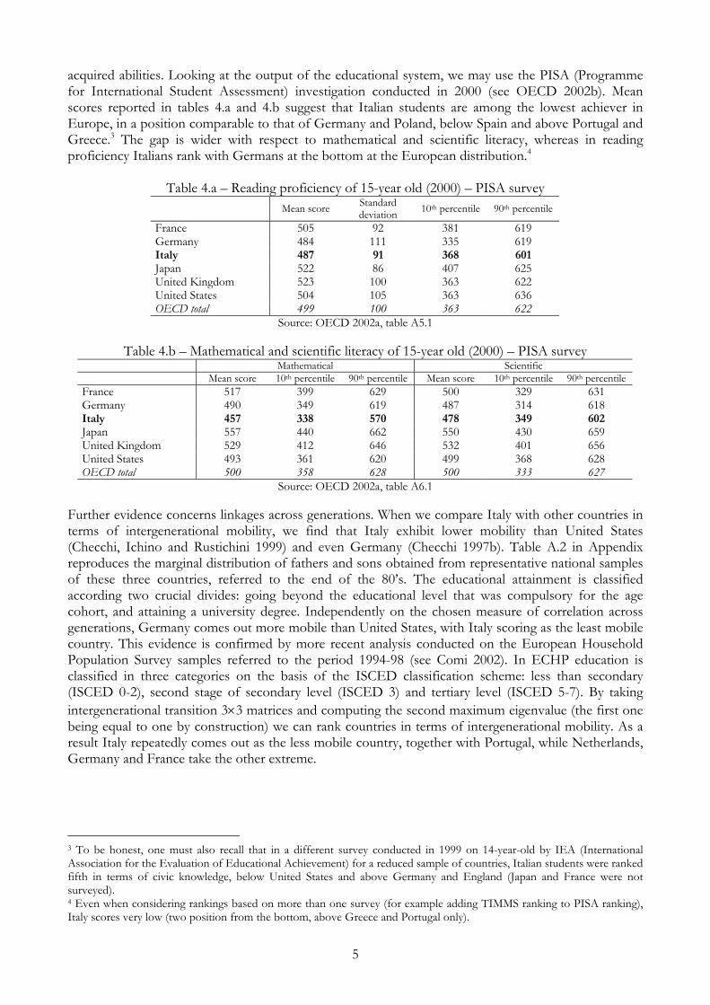
acquired abilities. Looking at the output of the educational system, we may use the PISA (Programme for International Student Assessment) investigation conducted in 2000 (see OECD 2002b). Mean scores reported in tables 4.a and 4.b suggest that Italian students are among the lowest achiever in Europe, in a position comparable to that of Germany and Poland, below Spain and above Portugal and Greece.3 The gap is wider with respect to mathematical and scientific literacy, whereas in reading proficiency Italians rank with Germans at the bottom at the European distribution.4

Table 4.a – Reading proficiency of 15-year old (2000) – PISA survey

Mean score Standard deviation 10th percentile 90th percentile

France 505 92 381 619 Germany 484 111 335 619 Italy 487 91 368 601 Japan 522 86 407 625 United Kingdom 523 100 363 622 United States 504 105 363 636 OECD total 499 100 363 622

Source: OECD 2002a, table A5.1

Table 4.b – Mathematical and scientific literacy of 15-year old (2000) – PISA survey Mathematical Scientific Mean score 10th percentile 90th percentile Mean score 10th percentile 90th percentileFrance 517 399 629 500 329 631 Germany 490 349 619 487 314 618 Italy 457 338 570 478 349 602 Japan 557 440 662 550 430 659 United Kingdom 529 412 646 532 401 656 United States 493 361 620 499 368 628 OECD total 500 358 628 500 333 627

Source: OECD 2002a, table A6.1 Further evidence concerns linkages across generations. When we compare Italy with other countries in terms of intergenerational mobility, we find that Italy exhibit lower mobility than United States (Checchi, Ichino and Rustichini 1999) and even Germany (Checchi 1997b). Table A.2 in Appendix reproduces the marginal distribution of fathers and sons obtained from representative national samples of these three countries, referred to the end of the 80’s. The educational attainment is classified according two crucial divides: going beyond the educational level that was compulsory for the age cohort, and attaining a university degree. Independently on the chosen measure of correlation across generations, Germany comes out more mobile than United States, with Italy scoring as the least mobile country. This evidence is confirmed by more recent analysis conducted on the European Household Population Survey samples referred to the period 1994-98 (see Comi 2002). In ECHP education is classified in three categories on the basis of the ISCED classification scheme: less than secondary (ISCED 0-2), second stage of secondary level (ISCED 3) and tertiary level (ISCED 5-7). By taking intergenerational transition 3×3 matrices and computing the second maximum eigenvalue (the first one being equal to one by construction) we can rank countries in terms of intergenerational mobility. As a result Italy repeatedly comes out as the less mobile country, together with Portugal, while Netherlands, Germany and France take the other extreme.

3 To be honest, one must also recall that in a different survey conducted in 1999 on 14-year-old by IEA (International Association for the Evaluation of Educational Achievement) for a reduced sample of countries, Italian students were ranked fifth in terms of civic knowledge, below United States and above Germany and England (Japan and France were not surveyed). 4 Even when considering rankings based on more than one survey (for example adding TIMMS ranking to PISA ranking), Italy scores very low (two position from the bottom, above Greece and Portugal only).

6

Table 5 - Intergenerational mobility matrices in educational attainment father-son mother-son father-daughter mother-daughter Country

eigenvalues rank eigenvalues rank eigenvalues rank eigenvalues rank Germany 0.147 3 0,620 7 0.171 5 0.663 7 Denmark 0.190 4 0,655 9 -0.097 3 0.586 3 Netherlands 0.130 1 0,638 8 0.080 2 0.600 4 Belgium 0.258 8 0,485 4 0.113 4 0.580 2 France 0.468 10 0,446 2 0.213 7 0.517 1 United Kingdom 0.144 2 0,678 11 0.016 1 0.666 8 Ireland 0.207 5 0,485 3 0.276 8 0.635 6 Italy 0.233 7 0,642 10 0.412 10 0.671 10 Greece 0.213 6 0,525 5 0.199 6 0.601 5 Spain 0.333 9 0,369 1 0.336 9 0.669 9 Portugal 0.642 11 0,625 6 0.541 11 0.725 11

Source: Comi 2002, table 6 and 7

One may object that the specific measure adopted here to rank countries is too specific. Checchi and Dardanoni (2002) use comparative samples of countries surveyed in the mid-seventies and measure intergenerational mobility in years of acquired education using nine different indices of mobility. Italy (surveyed in 1975) comes out as one of the least mobile countries, at least in terms of absolute (or structural) mobility, whereas it is much more mobile when looking at relative (or exchange) mobility. The authors have also repeated a similar exercise on more recent Italian data. By combining the SHIW (Survey of Household Incomes and Wealth) conducted by the Bank of Italy for 1993, 1995 and 1998 (to increase sample size) and collecting information on educational achievements of household heads and his/her parents, they obtain alternative measures of mobility for each age cohort, reported in figure 1. One may notice a strikingly different behaviour of the various classes of mobility indices, which can be explained by the different weight given to the structural and exchange component of mobility by the different indices. There are two conflicting forces at work: fathers and sons marginal distributions become “closer” over time (structural mobility declines) while becoming also less positively associated (exchange mobility increases). The net effect depends on the chosen class of indices. It is worth noticing that both groups of indicators point to an increase of mobility for the generation born during the 50’s. This is probably entirely attributable to the educational reform introduced in 1960 in Italy, which extended compulsory education from 5 to 8 years and unified the lower secondary school. This educational push was at the same time an increase in absolute mobility (for it was compulsory and was legally enforced, thanks to the construction of several school buildings) and in relative mobility, because it allowed the sons’ generation to gain access to secondary schools (which were originally de facto prevented by the existence of vocational schools driving children from peasant families directly to work after 5 years of primary school). This educational push attenuates for generations born in the 60’s, but the trend in relative mobility is rising.

7

Figure 1 – Mobility across cohorts – Italy 1993-95-98 – years of education

Alternative measures of educational achievement mobility

(mea

n) in

dex1

absolute mobility: index 1birth year

1930 1940 19501950 1960 1970

4.5

5

5.5

(mea

n) in

dex2

absolute mobility: index2birth year

1930 1940 19501950 1960 1970

30

35

40

45

(mea

n) in

dex3

relative mobility: index 3birth year

1930 1940 19501950 1960 1970

.45

.5

.55

(mea

n) in

dex4

relative mobility: index 4birth year

1930 1940 19501950 1960 1970

.5

1

1.5

2

2.5

(mea

n) in

dex5

relative mobility: index 5birth year

1930 1940 19501950 1960 1970

.4

.45

.5

.55

(mea

n) in

dex6

relative mobility: index 6birth year

1930 1940 19501950 1960 1970

.4

.45

.5

.55

(mea

n) in

dex7

relative mobility: index 7birth year

1930 1940 19501950 1960 1970

.06

.07

.08

.09

(mea

n) in

dex8

relative mobility: index 8birth year

1930 1940 19501950 1960 1970

.18

.2

.22

.24

(mea

n) in

dex9

mobility: index 9birth year

1930 1940 19501950 1960 1970

.3

.4

.5

.6

We can now summarise the aggregate empirical evidence concerning Italy. This country is characterised by low educational achievement when compared to other European countries with similar levels of development; the gap is sizeable with respect to tertiary education, while it is reducing (at a slow pace) in the case of upper secondary education. In terms of literacy, Italian youngsters rank below the OECD averages, despite the high rates of drop-out that should sort better students to remain in schools. The crucial question is therefore: why do Italians remain less at school than other Europeans ? and why, when they do, do they not get satisfactory results in terms of acquired abilities ? Among others, one potential explanation has to do with the limiting role of family background. Even if more recent cohorts face better prospects in terms of educational attainment, educational choices in Italy are strongly affected by parental education, and this may represent one of the most (if not the most) relevant factors hindering educational choice in Italy. The next section discusses competing potential explanations, whereas section 4 provides additional evidence on the issue of intergenerational dependence. 3. Potential explanations

3.1 – Wrong expectations

The first explanation that comes to mind about low educational attainment concerns the expected returns to education. If the expected flow of earnings has a net present value that is not greater than the current cost mainly constituted by forgone income, then standard theory predicts that an educational investment is not worth undertaking (Ben-Porath 1967). This explanation is hard to verify, since it is based on expectations of future rates of returns. Since return rates are equilibrium prices, it requires the prediction of future trends in demand and supply of human capital, a severe task in a period of technological change. As any expectation formation, it is likely to be affected by band-wagon effects, especially under static expectation formation. When current relative earnings for a specific profession are high, it is easy to predict that enrolment rates will rise in the specific school (or faculty) that gives

8

access to that profession.5 This phenomenon has already been noted with respect to the supply of engineers in the United States in the 60’s (Freeman 1986). Similar evidence could also be observed with respect to the Italian case, especially at university level (where perhaps the investment content of this educational choice is more accurate). With respect to secondary enrolment, reported in figure 2, some fluctuations are observable only with respect to teaching schools (istituti magistrali), whereas other enrolment shares suggest a relative decline in generalist and academic-oriented high schools counterbalanced by the expansion of technical and vocational enrolment.6 On the contrary, with respect to university enrolment shares shown in figure 3, we observe pronounced fluctuations in enrolment share: a first wave is detectable with respect to humanistic faculties at the end of the 60’s (probably following an intensification in public hiring for teachers), a subsequent wave can be observed in medical schools during the 70’s, while in recent years a rising trends is observed by Law and Economics faculties.

5 With this respect, the legal requirement of affiliation to a professional association, by restricting the access to the profession (and increasing the rent associated to it), should reduce the enrolment fluctuations. 6 The relative decline in high school enrolment is only the statistical artefact of even stronger rise of enrolments in vocational and technical schools: in fact the absolute number of students enrolled in high schools rose from 171.017 in 1945-46 to 753.476 in 1994-95, whereas total enrolment in technical schools grew over the same period from 105.329 to 1.159.569.

9

Figure 2 – Enrolment shares by secondary school types – Italy 1945-1996 sh

are

in s

econ

dary

enr

olm

ents

high schools - licei classici and scientificiyear

1946 1956 1966 1976 1986 1996

.2

.3

.4

.5

shar

e in

sec

onda

ry e

nrol

men

ts

4-year humanities secondary schoolsyear

teaching schools art schools

1946 1956 1966 1976 1986 1996

0

.05

.1

.15

.2

shar

e in

sec

onda

ry e

nrol

men

ts

3-year vocational schools - istituti professionaliyear

1946 1956 1966 1976 1986 1996

.05

.1

.15

.2

shar

e in

sec

onda

ry e

nrol

men

ts

5-year technical schools - istituti tecniciyear

1946 1956 1966 1976 1986 1996

.25

.3

.35

.4

.45

Figure 3 – Enrolment shares by faculties – Italy 1866-1997

shar

e in

uni

vers

ity e

nrol

men

ts

mathematics, physics and other sciences - engineering created in 1890year

scientist engineer

1866 1876 1886 1896 1906 1916 1926 1936 1946 1956 1966 1976 1986 1996

.1

.2

.3

.4

shar

e in

uni

vers

ity e

nrol

men

ts

medical schools and agrarian sciencesyear

medical agrarian sciences

1866 1876 1886 1896 1906 1916 1926 1936 1946 1956 1966 1976 1986 1996

0

.1

.2

.3

.4

shar

e in

uni

vers

ity e

nrol

men

ts

law, political sciences, economics and sociologyyear

law social sciences

1866 1876 1886 1896 1906 1916 1926 1936 1946 1956 1966 1976 1986 1996

0

.2

.4

.6

shar

e in

uni

vers

ity e

nrol

men

ts

literature, history and philosophyyear

1866 1876 1886 1896 1906 1916 1926 1936 1946 1956 1966 1976 1986 1996

0

.1

.2

.3

.4

10

These fluctuations signal the possibility of wrong expectations about future labour outcomes of educational choice. Direct test on expectations of college students has been conducted by Brunello, Lucifora and Winter-Ebner 2002 over 50 faculties of 32 universities in 10 European countries, with an overall sample of 6.829 college students. Generally speaking, they find that college students tend to overpredict their expected gain at start of career; but Italian students do not worse than students from other countries, both in terms of average errors and of dispersion of expectations. This evidence does not constitute a fully convincing explanation of low educational attainment. If expectations over labour market prospects were systematically biased at initial enrolment, and information accrues during the years of attendance, we could observe high drop-out rates as long as expectations are revised downwards.7 However wrong expectations per se cannot account for the intergenerational persistence in educational choice, unless we were inclined to accept an expectation formation theory where parental education has strong bearing.8

3.2 – Low returns to education

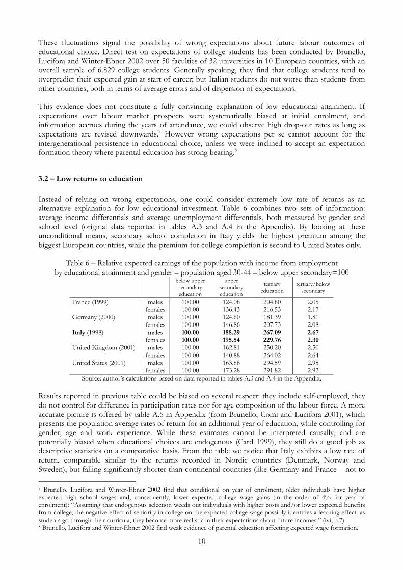
Instead of relying on wrong expectations, one could consider extremely low rate of returns as an alternative explanation for low educational investment. Table 6 combines two sets of information: average income differentials and average unemployment differentials, both measured by gender and school level (original data reported in tables A.3 and A.4 in the Appendix). By looking at these unconditional means, secondary school completion in Italy yields the highest premium among the biggest European countries, while the premium for college completion is second to United States only.

Table 6 – Relative expected earnings of the population with income from employment by educational attainment and gender – population aged 30-44 – below upper secondary=100

below upper secondary education

upper secondary education

tertiary education

tertiary/below secondary

France (1999) males 100.00 124.08 204.80 2.05 females 100.00 136.43 216.53 2.17 Germany (2000) males 100.00 124.60 181.39 1.81 females 100.00 146.86 207.73 2.08 Italy (1998) males 100.00 188.29 267.09 2.67 females 100.00 195.54 229.76 2.30 United Kingdom (2001) males 100.00 162.81 250.20 2.50 females 100.00 140.88 264.02 2.64 United States (2001) males 100.00 163.88 294.59 2.95 females 100.00 173.28 291.82 2.92

Source: author’s calculations based on data reported in tables A.3 and A.4 in the Appendix. Results reported in previous table could be biased on several respect: they include self-employed, they do not control for difference in participation rates nor for age composition of the labour force. A more accurate picture is offered by table A.5 in Appendix (from Brunello, Comi and Lucifora 2001), which presents the population average rates of return for an additional year of education, while controlling for gender, age and work experience. While these estimates cannot be interpreted causally, and are potentially biased when educational choices are endogenous (Card 1999), they still do a good job as descriptive statistics on a comparative basis. From the table we notice that Italy exhibits a low rate of return, comparable similar to the returns recorded in Nordic countries (Denmark, Norway and Sweden), but falling significantly shorter than continental countries (like Germany and France – not to 7 Brunello, Lucifora and Winter-Ebner 2002 find that conditional on year of enrolment, older individuals have higher expected high school wages and, consequently, lower expected college wage gains (in the order of 4% for year of enrolment): “Assuming that endogenous selection weeds out individuals with higher costs and/or lower expected benefits from college, the negative effect of seniority in college on the expected college wage possibly identifies a learning effect: as students go through their curricula, they become more realistic in their expectations about future incomes.” (ivi, p.7). 8 Brunello, Lucifora and Winter-Ebner 2002 find weak evidence of parental education affecting expected wage formation.

11

speak of the more liberalised labour market in United Kingdom). The association of Italy with Nordic countries may have something to do with unionisation of labour markets. As a tentative exercise, in figure A.1 in the Appendix we have cross-plotted the estimated returns with the average union membership for the corresponding period/country. The graph suggests a negative correlation between these two variables, since returns to education tend to be lower in countries where unions have a larger constituency and may keep a stronger hold in wage determination, compressing wage distribution (DiNardo, Fortin and Lemieux 1996).9 Nevertheless, the other Nordic countries still experience higher educational attainment than Italy, thus weakening the explanatory potential of returns to education. In any case, the structure of educational returns offers the right structure of incentives to proceed further in the academic ladder. In order to assess it, we pull together the SHIW surveys for the most recent decade (1933, 1995, 1998 and 2000) reaching a sample of 51.105 individuals aged between 25 and 65, among which 21939 have a positive labour income from dependent employment (see table A.7 in the Appendix for descriptive statistics of this sample).10 We have computed the yearly gross income from declared net incomes, by taking into account family compositions and relevant fiscal codes applicable to the year, in order to correct for potential bias due to progressivity of income taxation. Using sample weighed ordinary least squares and taking into account heteroskedasticity and clustering of errors, we then estimate the relative returns of different educational certificates, by progressively controlling for experience (linear and squared), gender, marital status (1st and 4th columns), whether employed part-time or full-time, whether employed the full year, the number of months worked (2nd and 5th columns), town size, region of birth, region of residence and cohorts effects (3rd and 6th columns – see table A.8 in the Appendix). The second three columns introduce parental education as additional controls. We take the most conservative estimates reported in the 6th column of table A.8 in the Appendix, and we compute the annualised rate of return for any educational levels, leaving the absence of educational credential as the reference case.11 As we can see from table 7, the yearly rate of return is increasing with the educational attainment: completing primary school is by now statistically indistinguishable from being illiterate, while completing lower secondary school is on the hedge of statistical significance. On the contrary, proceeding beyond compulsory education still provides a reasonable incentive.12

9 Once again, we are uncertain about the direction of causation: if returns to education reflect skill distribution, low returns could be the endogenous result of a compressed skill distribution. If at the same time low skill workers are more likely to unionise, then figure A.1 represents a case of spurious correlation. 10 We neglect incomes from self-employment, since they are plagued with under-reporting. See Cannari and D’Alessio 1993 and Brandolini 1999

11 Data in table 7 have been obtained as ( ) 100111

⋅

−

β+ ini where iβ is the dummy coefficient associated to

educational level i and in is the standard length of educational level i ; we have considered 5 years for primary school, 3 years for lower secondary school, 5 years for upper secondary school and 5 year for university degree. Unfortunately we do not have information about repetitions and/or failed attempt to proceed further in the educational career; as a consequence the estimates reported in table 7 are upward biased. However, since educational choices are endogenous and controlling for parental education does not solve the problem entirely, the same estimates could be downward biased. Since these estimates are meant as descriptive statistics to obtain relative return rates, if the direction of these biases do not change across different educational levels the comparisons remain meaningful. 12 The estimated coefficients are in the right order of magnitude for the Italian case, as can be checked by comparing with a set of previous estimates reported in tables A.9 and A.10 in the Appendix (showing OLS and IV previous estimates respectively). However Blöndal, Field and Girouard 2002 presents estimates by school level where the (internal) return rate for Italy declines when passing from upper secondary to tertiary education (see table A.6 in the Appendix); the difference can be accounted by the different methodology used to obtain the estimates.

12

Table 7 – Annualised rate of return of different educational levels - Italy 1993-1995-1998-2000

yearly rate of return (%)

Primary school 0.250 Lower secondary school 3.803 Upper secondary school 6.033 University degree 8.939

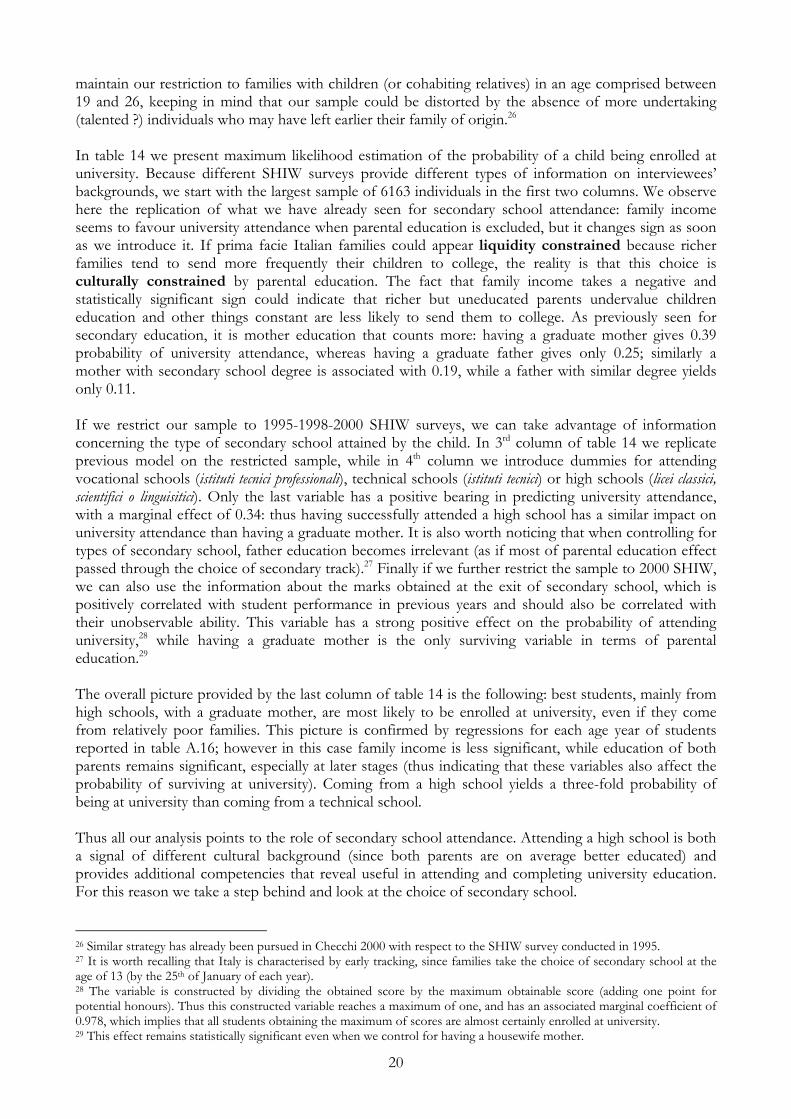
Source: see 6th column of table A.8 From table A.8 in the Appendix we also notice that a significant portion of differential returns are accounted by differences in working hours and local labour market and cohort effects, thus suggesting that different educational attainments could have additional returns in terms of easier employability and/or better access to full-time employment. This evidence suggests a better scrutiny of the returns associated to different secondary school degrees. Even if in principle the access to university is assured to any person holding a 5-year secondary school certificates (since the educational reform introduced in 1969), the Italian secondary school system should be classified as stratified, because transition rates to college are heavily dependent on the type of secondary school attained.13 As a consequence, it would be interesting to measure the relative return of different tracks, possibly on some equal grounds. In SHIW the information concerning the type of secondary school attained is available only starting with 1995, but unfortunately is not reported for individuals attaining a university degree.14 Thus it is possible to estimate the relative returns of different types of secondary school conditional on not accessing and/or not completing a university curriculum: in this way we are likely to measure relative returns of secondary schools for individuals in the bottom tail of unobservable ability distribution. In table A.11 in the Appendix we have estimated the relative return of different secondary degrees, while table A.12 in the Appendix provides estimates of the relative contribution of the same degrees with respect to the probability of entering the labour force and employment. By looking to the estimated coefficients, it looks as if the type of secondary school attended does not make any difference in terms of relative earnings,15 whereas they make a difference in terms of labour market participation. Having attended a generalist high school without proceeding further to the university is negatively correlated with the probability of entering the labour force, as indicated by the highly negative coefficient associated with this dummy. Overall, we conclude this section by claiming that Italy is characterised by lower return to education than other European countries, but the incentive structure is correctly oriented, because it seems to favour the progress to further education. However wrong choices (like attending a high school without continuing for a university degree), possibly due to early tracking, are subsequently penalised in the labour market, not in terms of monetary rewards but in terms of likelihood of entrance in the labour force. Nonetheless, as argued before with respect to wrong expectations, the risk of taking a wrong choice does not seem to constitute the main obstacle to educational investment.

3.3 – Limited (public) resources invested in education

A third potential explanation that can be put forward to explain the low educational attainment of Italians comes from limited resources invested in education. However, by observing the evidence reported in table 8 we perceive that Italy spends more than most of its competitor countries up to

13 Different opinion is contained in Shavit and Muller 1998, where they classify only Germany, Austria, Switzerland and the Netherlands as stratified. 14 The SHIW questionnaire asks information about the highest educational attainment only, neglecting the intermediate ones. In addition this variable is missing for 9.4% of interviewees declaring to possess a 5-year secondary school degree. More information is obtainable from retrospective surveys like the one reported in Schizzerotto 2002. 15 A test on joint significance of type of secondary degree dummies does not reject the hypothesis of all coefficients being not different from zero.

13

secondary education, whereas the true expenditure deficit materialises at tertiary education.16 A typical indicator of resources involved in education, the student/teacher ratio, confirms this. Looking at table 9, we see that Italy is characterised by the lowest student to teacher ratio up to secondary education, but at the same time has the second to highest ratio in tertiary education, after Greece.

Table 8 – Expenditure per student by educational level (1999) – PPP US dollars

pre-primary education

primary education

all secondary education

all tertiary education

France 3901 4139 7152 7867 Germany 4937 3818 6603 10393 Italy 5133 5354 6518 7552 Japan 3154 5240 6039 10278 United Kingdom 6233 3627 5608 9554 United States 6692 6582 8157 19220 OECD average 3847 4148 5465 9210

Source: OECD 2002a, table B1.1

Table 9 – Ratio of students to teaching staff – public and private education (2000)

pre-primary education

primary education

lower secondary education

upper secondary education

all tertiary education

France 19.1 19.8 14.7 10.4 18.3 Germany 23.6 19.8 15.7 13.9 12.1 Italy 13.0 11.0 10.4 10.2 22.8 Japan 18.8 20.9 16.8 14.0 13.1 United Kingdom 21.0 21.2 17.6 12.5 17.6 United States 18.7 15.8 16.3 14.1 13.5 OECD average 15.5 17.7 15.0 13.9 14.7

Source: OECD 2002a, table D2.2 But we have already noticed that the educational gap already materialises at secondary school level (see table 2 above), where the amount of resources invested in education in Italy, at least with respect to teachers, is still higher than the OECD average. In order to assess the relative contribution of school resources to educational attainment, in the sequel we have replicated the analysis developed in Brunello, Checchi and Comi (2002). In Italy there are no data on school quality at the individual level that covers a nationally representative sample. Therefore, we used aggregate measures of quality based on region and year of birth.17 We collected data on school quality for each of the 20 Italian regions and for any other year (due to the limited short term variability of the data), restricting our analysis to individuals born in between 1940 and 1970. With respect to educational resources, we start in 1944, when the oldest cohorts could start kindergarten, and end in 1989, when the youngest cohort could have completed upper secondary education. To illustrate, to an individual born in 1945 who went to kindergarten between 1948 and 1951, to primary school between 1951 and 1956, to junior high school between 1956 and 1958 and to upper secondary school between 1958 and 1963 we attribute the resource measures associated to each type of school in the same sub-period. To reduce the number of potential regressors, these measures are then aggregated across school levels, using participation rates as weights. In this way, each individual is given the average of educational resources s/he could have experienced had s/he attended school up to secondary level. The justification of this procedure is provided by the fact that the choice of not attending a further stage of education can be affected by the level of resources there available. The underlying assumption is that the relevant measure of school quality is associated to the region/year of birth, because most individuals completed their schooling, from less than primary to

16 Table A.13 in Appendix exhibit the ratio of expenditure with national output per capita. 17 Due to privacy restrictions, the SHIW survey only makes available to researchers information on the region of birth.

14

upper secondary, in the same region.18 We collected regional data on seven indicators of school resources, as reported in table 10. We have excluded college education, because individual migration between regions to enrol in college has been the standard pattern during most of the period under study.

Table 10 – Descriptive statistics of aggregate indicators of school resources experienced by people born in Italy over the period 1940-1970

variable name definition mean standard

deviation minimum maximum

G0 enrolment rate 61.84 15.16 0.32 (Basilicata 1942) 0.88 (Piedmont 1960) G1 students per teacher 20.96 4.91 13.28 (Umbria 1968) 38.92 (Sardinia 1942) G2 students per school 202.29 58.13 80.22 (Valle d’Aosta 1942) 351.68 (Puglia 1946) G3 class size 25.97 6.41 17.78 (Umbria 1968) 49.65 (Sardinia 1942) G4 private schools share 22.30 6.01 0.08 (Basilicata 1952) 0.40 (Liguria 1946) G5 tenured/untenured teachers 88.67 72.50 0.10 (AbruzzoMolise 1968) 6.70 (Basilicata 1950) G6 class size – private schools 25.70 2.06 19.24 (Umbria 1956) 31.02 (Puglia 1942) G7 selectivity (repetition rate) 9.90 4.61 2.99 (Umbria 1970) 25.48 (Sardinia 1944)

Figure 4 plots the aggregate indicators with ± one standard deviation computed across regions. Over the sample period it is easy to notice that participation rate rose, the student per teacher and class size declined in public schools (with a reduction in variation across regions), but remained almost constant in private schools. Private school share remained constant, while the proportion of untenured teachers and the repetition rates declined.

Figure 4 – Aggregate indicators of school resources

aggregate indicators - Italy

participation ratebirth year

aggregate:enrolment +1 sd -1 sd

1940 1950 1960 1970

.4

.6

.8

student/teacherbirth year

aggregate:student/teacher +1 sd -1 sd

1940 1950 1960 1970

15

20

25

30

35

school sizebirth year

aggregate publ:school size +1 sd -1 sd

1940 1950 1960 1970

100

150

200

250

300

class sizebirth year

aggregate publ:class size +1 sd -1 sd

1940 1950 1960 1970

20

25

30

35

40

private school sharebirth year

aggregate:private schools +1 sd -1 sd

1940 1950 1960 1970

.15

.2

.25

.3

.35

untenured/tenured teachersbirth year

aggregate:untenured/tenured tea +1 sd -1 sd

1940 1950 1960 1970

0

1

2

3

class size - privatebirth year

aggregate priv:class size +1 sd -1 sd

1940 1950 1960 1970

22

24

26

28

30

repetition ratebirth year

aggregate publ:selectivity +1 sd -1 sd

1940 1950 1960 1970

0

.05

.1

.15

.2

18 The plausibility of assigning to each individual the school quality of the region of birth could obviously be questioned. In the absence of individual information on the age when migration eventually took place, we can only control the percentage of individuals older than 19 who live in the same region of birth. In our sample, the 84.4% of individual was residing in the same region where they were born, but the percentage increases with younger cohorts (from 80.9% of the oldest to 90.1% of the youngest).

15

We have used these seven indicators of school resources to analyse potential correlation with educational choices of individuals in our sample. In addition to gender, region of birth, region of residence and cohort dummies, we have introduced parental education (measured by the number of years of the maximum educational attainment in the couple of parents) and the interaction between the resource indicator and parental education. An ordered probit model is reported in table 11, to account for ordinality of educational attainment, whereas an ordinary least square model (converting the degree in years of schooling) is reported in table A.14 in the Appendix.19

Table 11 – Maximum likelihood ordered probit estimation of educational attainment

weight cluster – SHIW surveys 1993-95-98-00 (robust standard errors – z-statistics in parentheses with p<0.05 = *, p<0.01 = **)

------------------------------------------------------------------------------------------- Resour: G1 G2 G3 G4 G5 G6 G7 # obs : 32884 32884 32884 28498 32884 32884 25649 Depvar: edyear edyear edyear edyear edyear edyear edyear ------------------------------------------------------------------------------------------- resources -0.0440** -0.0011~ -0.0295** -0.9617 -0.0416 -0.0484** -2.6681* (-6.89) (-2.20) (-6.51) (-1.12) (-0.83) (-3.33) (-1.99) parental 0.0554** 0.1630** 0.0587** 0.1305** 0.1395** 0.0833 0.1136** education (4.17) (10.79) (3.91) (8.12) (23.91) (1.57) (13.50) resour× 0.0049** 0.0000 0.0038** 0.1116 0.0203** 0.0028 0.4521** par.educ. (7.35) (-0.43) (6.32) (1.67) (3.26) (1.38) (5.68) Gender Yes Yes Yes Yes Yes Yes Yes Cohort Yes Yes Yes Yes Yes Yes Yes Birth Yes Yes Yes Yes Yes Yes Yes Resid Yes Yes Yes Yes Yes Yes Yes ------------------------------------------------------------------------------------------- pseudoR² 0.135 0.132 0.135 0.124 0.133 0.132 0.127 ===========================================================================================

We notice that student/teacher ratio (G1) and class size (G3 for public schools and G6 for private schools) limit educational attainment of the generations educated in the aftermath of the Second World War. But this effect is attenuated for individuals coming from better-educated families. As expectable, parental education is highly correlated with children educational attainment. If we look at OLS regression coefficients (table A.14 in the Appendix) we can derive an iso-attainment relationship (i.e. the locus of all possible combinations of parental education and teachers available to students such that student educational attainment remains constant) . Take for example the first column, and consider that sample averages of G1 and parental education EDG (when missing observations are excluded) are respectively 20.96 and 5.82; then the elasticity of substitution (along an hypothetical iso-attainment curve) computed at sample means is given by

96.096.20

82.546.396.20

82.596.2082.5012.096.2011.0

96.2082.5012.082.5250.01

1=⋅=⋅

⋅⋅+⋅−⋅⋅+⋅

−=⋅GEDG

dEDGdG

Its interpretation is straightforward: an improvement of 10% in school resources (reducing two students per teacher) compensates almost one to one a 10% decline in parental education (something more than half a year of educational attainment of parents). Given the fact that years of education have risen (from an average of 8.08 for individuals born in the period 1940-45 to 11.35 for individuals born in 1965-70) together with parental education (from 4.61 to 7.60 over the same period) and school resources (the student/teacher ratio declined from 27.2 to 16.1), the relative contribution of parental 19 The number of cases is reduced in the case of G4 and G7 indicators because of lack of information during initial years for these variables.

16

education (+1.50, computing the interaction effect at sample averages) is greater than school resources effect (+0.44, computing again the interaction effect at sample averages). We can therefore conclude this section by stating that public resources invested in schooling do not seem to prevent educational investment. If any, they have had a positive effect (at least in terms of the number of teachers employed), helping to raise the educational attainment in the population for recent cohorts. However, we found that parental education has a stronger impact than public resources, thus eliciting the suspect that this can be the real limiting factor in educational attainment in Italy. 4. Additional evidence on family background In the previous section we have discussed competing explanations of the low educational investment in Italy, based on expectational errors, low returns and low resources. None of these explanations is capable to account for the pattern of behaviour described in section 2, where we have shown that drop-out rates during secondary and tertiary education and/or low transition rates at university are found responsible for the low educational attainment. Fort this reason, in this section we focus on educational choice within Italian families, in order to gain additional insights on the problem. Even if it is a common plea, it is always worth repeating that Italy lacks adequate statistical information to deal with this type of issues. In order to analyse educational choices, the appropriate data-set would consist of a panel of individuals repeatedly observed in the course of their educational career.20 To the best of my knowledge, such a data-set does not exist in Italy. Therefore we are forced to rely on repeatedly cross-sections as if they could provide similar information. The validity of the “as if” assumption is conditional to the stability of the environment we intend to analyse. This is not exactly the case of Italy in recent years, where a sweeping reform of secondary education has been approved (and never implemented) in 200021 and a profound reorganisation of the university system has started in 2001.22 Thus any analysis based on observed behaviours during the previous decade may prove false in the light of a sort of Lucas’ critique: by changing the environment the agents are forced to redefine their optimal choices. Nonetheless, we believe that some problems are so deeply rooted in the Italian society that they will persist further of recent reforms. For these reasons, having these caveats in mind, we now proceed in our analysis. We take as our unity of analysis all individuals younger than 30 year old that belong to our sample, obtained by combining the SHIW surveys conducted in 1993,1995, 1998 and 2000. Above mentioned reforms were already announced, especially during the last survey, but these reforms are slow in taking place, and we feel safe in assuming that families interviewed in different surveys faced an identical environment with respect to educational choices.23 For each individual we know his/her actual position (whether student, first job seeker, unemployed, employed or out of labour force), maximum educational attainment achieved so far, and all relevant information concerning the family background (family composition, family income, parental education). We are therefore able to investigate whether 20 A good example is provided by the British NCDS (National Child Development Survey), where a cohort of individual born in the same week of 1958 has been interviewed 6 times, collecting information on school resources, parents attitudes, social environment, up to the entrance in the labour market. See Dearden, Ferri and Meghir 1998. 21 Legge quadro n.30 published in the Gazzetta Ufficiale on 10/2/2000 (better known as Berlinguer-DeMauro reform, by the name of the Ministers of Public Education), and now to be replaced by proposal n.1306 “Delega al governo per la definizione delle norme generali sull’istruzione e dei livelli essenziali delle prestazioni in materia di istruzione e formazione professionale” (also known as Moratti reform). 22 In application of the “Regolamento recante norme concernenti l’autonomia didattica degli atenei” (published in the Gazzetta Ufficiale on 4/1/2000), better known as “3+2” reform, since it introduces a 3-year degree equivalent to a B.A. followed by a 2-year M.A., enlarging the class of potential degrees awardable by each university. 23 It is also important to recall that the SHIW survey contains a panel component (equal to 43.1% of the sample in 1993, 44.9% in 1995, 36.7% in 1998 and 49.2% in 2000), that may distort our analysis if it constitutes a biased sample of the entire population (due for example to attrition). However, as long as all statistical analysis correct for sample weights, the problem is attenuated.

17

and how much family background affect current status. Unfortunately we ignore most of the educational career of each individual (whether s/he has never repeated one year, any change of school, any failed attempt, the marks obtained in previous school levels). Part of this information has to be obtained by other data-set. Let us start with the actual status distribution by age, as shown in figure 5, that virtually replicates the educational careers from aggregate data reported in table 3 . While 88.8% of the relevant cohort passes to upper secondary school at the age of 15, they shrink to 54.8% by the age of 19; 34% of potential graduates from secondary school vanishes during its course, mainly in the passage between first and second year. Similarly, 45.9% is enrolled at university at the age of 20, but only two third of them still persist after 4 years. When we look at territorial disaggregation (plotted in figure A.2) we discover that the lack of secondary school attendance is concentrated in Southern regions, and even more in the Islands: while 80% is still in school at the age of 18 in North and Centre, the corresponding figure is 70% in Southern regions and almost 60% for the Islands. It is also interesting to note that school attendance is on average five points higher for girls than for boys, and the difference disappears around the age of 24. If we now consider secondary school attendance in more detail, we lack information about educational career during primary and lower secondary schools; more specifically, we do not observe repetitions and failed attempts, nor we have information about marks. We know that compulsory education extends now to 15 years old , and for regular students it implies compulsory enrolment to first year of secondary school. However, we have seen that drop-out rates reduces that number in a couple of years. We consider three alternative conditions in which we can register youngster: in school (if they are classified as “student”), in the labour market (if they are recorder as “employed” or “unemployed” or “first job seeker”) and out of labour market (if they are classified as “housewife”, “rentier”, “invalidity pension” or “on military duty”). Given the fact that these choices are mutually excludable and are all potentially possible, in table 12 we have estimated a multinomial logit model for this choice.

Figure 5 – Current status by age – Italy 1993-95-98-2000

perc

ent

age0

.2

.4

.6

.8

1

in school seeking a job unemployed employed out of labour force

4 5 6 7 8 9 10 11 12 13 14 15 16 17 18 19 20 21 22 23 24 25 26 27 28 29 30

18

Table 12 – Maximum likelihood multinomial logit for youngsters’ condition weight cluster – SHIW surveys 1993-95-98-00 –

(relative risk ratios – robust standard errors – z-statistics in parentheses with p<0.05 = *, p<0.01 = **) Individuals coded as “child” or “relative”, aged between 15 and 19 – “out of labour force” as comparison case

------------------------------------------ # obs : 6100 6100 6100 ------------------------------------------ in school 74.60 employed/unemployed 22.62 out of labour force 2.78 ------------------------------------------

in school female 0.532* 0.564 0.587 (-1.80) (-1.66) (-1.53) age 0.697** 0.664** 0.682** (-3.53) (-4.24) (-3.94) log eq. 1.987** 1.207 fam.income (4.95) (1.19) father 4.629** up.secnd. (3.31) father 1.032 college (0.03) mother 16.41** up.secnd. (4.38) mother 62.73** college (3.86)

employed/unemployed/first job seeker

female 0.360** 0.365** 0.364** (-2.58) (-2.54) (-2.53) age 1.136 1.122 1.130 (1.36) (1.26) (1.37) log eq. 0.973 1.051 fam.income (-0.24) (0.33) father 0.751 up.secnd. (-0.69) father 0.132* college (-2.00) mother 1.693 up.secnd. (0.81) mother 1.036 college (0.03) ------------------------------------------ pseudoR² 0.098 0.128 0.242 ========================================== Note: macro-regions of residence and town size are included as additional regressors in all specifications.

Among potential explanatory variables, we have considered gender, age, macro-region of residence and town size; family background is measured by total family income (equivalised by a standard equivalence scale, that is divided by the square root of number of family components) and by educational attainments of both parents. Looking at statistically significant coefficients, it seems as family income favours staying in school, whereas the age works against it. However, when we look at table A.15 in the Appendix that decomposes the same model by each age year of the interviewee, we see that family income is crucial in determining school attendance only for the initial year (i.e. at age of 15), whereas educational attainment of both parents (especially if one or the other has completed secondary school) is important for permanence in school (and affects negatively the probability of entering the labour force). Territorial and/or town size dummies are almost always insignificant. Thus family income

19

comes out significant only because it is positively correlated with parental education: when we control for it (as done in 3rd column of table 12), we observe family income becoming statistically insignificant, while educational attainment of both parents (but in particular of the mother) are crucial in staying in secondary school. Overall the estimated model has a reduced explanatory power; its main weakness comes from our inability to control for the type of secondary school attained, since it is easy to suspect that different secondary tracks have different degrees of difficulty and pursue different policies of screening students. On the contrary, when we look at university attendance we identify potential university students according to two criteria: aged older than 18 (which represents the minimum age for a child starting at 5 and completing 5 years of primary, 3 years of lower secondary and 5 years of upper secondary school)24 and possessing a 5-year secondary school degree (diploma di maturità). Despite a legal duration of 4 to 6 years (depending on the subject), the median duration for the attainment of a bachelor degree in Italy is 7 years (see Istat 2000 and table 13 computed from the same data-set).

Table 13 – Effective years of duration for university degree attainment – Italy – ISTAT graduate survey 1995

Subjects mean

legal duration

st.deviation legal

duration

median effective duration

mean effective duration

st.deviation effective duration

Sciences 4.01 0.11 6 6.94 2.71 Chemistry and Pharmacy 4.66 0.47 6 6.95 2.82 Geo-biology 4.17 0.38 7 7.63 3.06 Medical school 5.77 0.42 7 8.28 3.37 Engineering 4.99 0.03 7 7.73 2.50 Architecture 4.99 0.09 8 8.79 2.66 Agrarian sciences 4.83 0.36 7 8.21 2.72 Economics and Statistics 4.04 0.19 6 6.74 2.09 Political sciences 4.02 0.16 6 7.23 3.34 Law 4.02 0.15 6 7.04 2.64 Arts 4.02 0.14 7 7.61 3.67 Literature 4.02 0.14 7 7.38 3.09 Teaching 4.01 0.12 7 8.55 5.08 Psychology 4.92 0.26 6 6.71 2.72 Total 4.39 0.58 7 7.41 2.98

Source: representative sample of graduates in 1995 surveyed in 1998 - standard sample file “Inserimento professionale dei laureati dell’anno 1995 Indagine 1998” – Istat 2000

For this reason we have considered as potential enrolled at the university all individuals aged between 19 and 26, extremes included. This strategy introduces potential distortions because we do not have information about children who may have left home to attend university in a different city, and are not registered as cohabiting. However we know from other sources that Italy is characterised by late leaving of family cohabitation,25 due to high costs of living and absence of unemployment benefits. Looking at our data, we can infer information by looking at family composition. In a constant population with children not leaving family cohabitation, we should observe a roughly constant number of children at any (average) age of children. Under the same assumption when we notice a sharp decline, we can take it as indirect indication of the (average) family leaving age. By observing figure A.3 in the Appendix, we notice that this sharp decline occurs in our data set around an average age of children of 29 (even if it starts declining at the age of 20). On this indirect evidence (and in the absence of better alternative) we

24 Istat (1999) reports that in 1995 only one third (31.7%) of secondary school graduates completed that order of schooling by the age of 19, while all the other either repeated at least one year or changed type of secondary school, loosing one year. 25 In 1996 the 98.1% of young people aged 18-19 was cohabiting with the family of origin. The same percentage declines to 88.4% for people aged 20-24, 54.1% for people aged 25-29 and 21.6% for people aged 30-34. See Istat 1997, pg.224 ss.

20

maintain our restriction to families with children (or cohabiting relatives) in an age comprised between 19 and 26, keeping in mind that our sample could be distorted by the absence of more undertaking (talented ?) individuals who may have left earlier their family of origin.26 In table 14 we present maximum likelihood estimation of the probability of a child being enrolled at university. Because different SHIW surveys provide different types of information on interviewees’ backgrounds, we start with the largest sample of 6163 individuals in the first two columns. We observe here the replication of what we have already seen for secondary school attendance: family income seems to favour university attendance when parental education is excluded, but it changes sign as soon as we introduce it. If prima facie Italian families could appear liquidity constrained because richer families tend to send more frequently their children to college, the reality is that this choice is culturally constrained by parental education. The fact that family income takes a negative and statistically significant sign could indicate that richer but uneducated parents undervalue children education and other things constant are less likely to send them to college. As previously seen for secondary education, it is mother education that counts more: having a graduate mother gives 0.39 probability of university attendance, whereas having a graduate father gives only 0.25; similarly a mother with secondary school degree is associated with 0.19, while a father with similar degree yields only 0.11. If we restrict our sample to 1995-1998-2000 SHIW surveys, we can take advantage of information concerning the type of secondary school attained by the child. In 3rd column of table 14 we replicate previous model on the restricted sample, while in 4th column we introduce dummies for attending vocational schools (istituti tecnici professionali), technical schools (istituti tecnici) or high schools (licei classici, scientifici o linguisitici). Only the last variable has a positive bearing in predicting university attendance, with a marginal effect of 0.34: thus having successfully attended a high school has a similar impact on university attendance than having a graduate mother. It is also worth noticing that when controlling for types of secondary school, father education becomes irrelevant (as if most of parental education effect passed through the choice of secondary track).27 Finally if we further restrict the sample to 2000 SHIW, we can also use the information about the marks obtained at the exit of secondary school, which is positively correlated with student performance in previous years and should also be correlated with their unobservable ability. This variable has a strong positive effect on the probability of attending university,28 while having a graduate mother is the only surviving variable in terms of parental education.29 The overall picture provided by the last column of table 14 is the following: best students, mainly from high schools, with a graduate mother, are most likely to be enrolled at university, even if they come from relatively poor families. This picture is confirmed by regressions for each age year of students reported in table A.16; however in this case family income is less significant, while education of both parents remains significant, especially at later stages (thus indicating that these variables also affect the probability of surviving at university). Coming from a high school yields a three-fold probability of being at university than coming from a technical school. Thus all our analysis points to the role of secondary school attendance. Attending a high school is both a signal of different cultural background (since both parents are on average better educated) and provides additional competencies that reveal useful in attending and completing university education. For this reason we take a step behind and look at the choice of secondary school. 26 Similar strategy has already been pursued in Checchi 2000 with respect to the SHIW survey conducted in 1995. 27 It is worth recalling that Italy is characterised by early tracking, since families take the choice of secondary school at the age of 13 (by the 25th of January of each year). 28 The variable is constructed by dividing the obtained score by the maximum obtainable score (adding one point for potential honours). Thus this constructed variable reaches a maximum of one, and has an associated marginal coefficient of 0.978, which implies that all students obtaining the maximum of scores are almost certainly enrolled at university. 29 This effect remains statistically significant even when we control for having a housewife mother.

21

Table 14 – Maximum likelihood probit estimation of university attendance weight cluster – SHIW surveys 1993-95-98-00 – marginal effects

(robust standard errors – z-statistics in parentheses with p<0.05 = *, p<0.01 = **) Individuals coded as “child” or “relative”, aged between 19 and 25, with a secondary school degree

------------------------------------------------------------------------------- # obs : 6163 6163 3973 3973 1176 1176 Depvar: uni uni uni uni uni uni Sample yrs: 1993-95-98-00 1995-98-00 2000 ------------------------------------------------------------------------------- un.student 49.9 49.9 46.9 46.9 48.4 48.4 not studnt 50.1 50.1 53.1 53.1 51.6 51.6 ------------------------------------------------------------------------------- female 0.026 0.037* 0.012 -0.047* -0.030 -0.060 (1.65) (2.20) (0.60) (-2.18) (-0.73) (-1.42) age -0.059** -0.053** -0.052** -0.052** -0.060** -0.060** (-11.13) (-9.72) (-7.82) (-7.91) (-4.91) (-4.85) log eq. 0.068** -0.066** -0.069** -0.087** -0.104** -0.114** fam.income (3.81) (-3.70) (-3.15) (-4.03) (-2.77) (-3.05) father 0.110** 0.043 0.008 -0.062 -0.045 up.secnd (3.46) (1.03) (0.21) (-0.73) (-0.56) father 0.250** 0.187** 0.089 0.177 0.177 college (5.14) (3.26) (1.59) (1.52) (1.52) mother 0.193** 0.212** 0.177** 0.123 0.055 up.secnd (3.97) (3.21) (2.82) (1.09) (0.48) mother 0.395** 0.426** 0.357** 0.299** 0.248* college (6.78) (7.38) (5.29) (2.77) (2.13) vocational -0.129 -0.250* -0.232 up.second (-1.67) (-2.01) (-1.85) technical -0.001 -0.147 -0.124 up.second (-0.02) (1.30) (1.07) high school 0.439** 0.342** 0.355** (6.76) (3.24) (3.17) mark at exit 0.997** up.secnd.schl (5.05) Town Yes Yes Yes Yes Yes Yes Area Yes Yes Yes Yes Yes Yes ------------------------------------------------------------------------------- R² 0.05 0.121 0.123 0.235 0.291 0.325 =============================================================================== We obtain further information from a survey conducted by ISTAT (the Italian National Institute for Statistics) in 1998 over a nationally representative sample of 18.843 students who left successfully the secondary school in 1995.30 We must keep in mind that this sample is not representative of the entire student population, since students completing upper secondary schools are self-sorted. Nevertheless it is the only sample reporting information on previous schooling experience and parental background.31

30 We use the standard file of “Percorsi di studio e di lavoro dei diplomati - Indagine 1998”. Descriptive statistics are reported in table A.17. 31 We are only aware of another recent survey of the same type, conducted by Istituto Cattaneo and described in Gasperoni 1996. These data have been analysed in Checchi and Zollino 2001, in order to detect potential existence of peer effects.

22

We use these data to investigate how school experience and parental background interrelate in modelling the secondary school choice, which is then relevant in future university choices. Table 15 displays the existence of correlation between family cultural background (as proxied by educational attainment of parents) and evaluation of students obtained at the exit of lower secondary school. Children with parents who did not complete compulsory education are much more likely to achieve the lowest grade; at the opposite extreme, children from graduate parents are most likely to score the highest. It must be recalled that in the final year of lower secondary school (when children are aged 13) teachers provide counselling services (orientamento scolastico) to families in order to choose an appropriate secondary school for their children. This guidance and/or autonomous family choices seem based on past students’ performance, as it can be grasped from table 16: best students are typically directed to academic careers through high schools, while less brilliant students are addressed to vocational schools. Since table 15 suggests that parental education reflects into student performance, and table 16 indicates that this assessment is relevant to future destiny, it raises the question on how predetermined are the destiny of students conditional on parental education.

Table 15 – Judgment at the exit of lower secondary school (licenza media) by maximum educational attainment in the couple of parents – Italy ISTAT survey 1995 – weighed maximum educational attainment between father and mother

sufficient (sufficiente)

good (buono)

very good (distinto)

excellent (ottimo)

total

illiterate 46.66 33.40 16.15 3.79 0.80 primary school 41.40 27.43 18.60 12.57 16.81 lower secondary school 39.46 28.63 17.82 14.09 34.19 vocational school (2-3 years) 33.58 31.72 21.62 13.08 5.56 upper secondary school (4-5 years) 27.30 27.68 22.49 22.53 30.83 BA (3-year university degree) 24.10 18.94 28.79 28.18 0.76 MA (5-year university degree)-PhD 16.60 23.42 21.94 38.05 11.05 Total 33.08 27.69 20.14 19.10 100.00

Table 16 – Judgment at the exit of lower secondary school (licenza media) and choice of secondary school – Italy ISTAT survey 1995 – weighed

vocational school

(ist.profess.)

technical school

(ist.tecnico)

teaching school

(ist.magistrale)

high school (licei)

school of arts

(ist.artistici) sufficient (sufficiente) 28.61 49.66 8.40 8.01 5.32 good (buono) 12.71 53.75 8.91 21.03 3.60 very good (distinto) 5.04 44.84 6.84 40.83 2.45 excellent (ottimo) 1.47 26.38 5.10 65.89 1.16 Total 14.33 45.41 7.60 29.18 3.48

In order to assess the relative contribution of student performance at previous school level and parental background, in table 17 we have estimate a maximum likelihood multinomial logit model on the secondary school choice. In the first model (1st and 3rd column) we have considered personal information (gender, age, region of residence) and the judgment at the exit of lower secondary: this model suggests that girls with better judgments tend to be self-sorted into high schools. In the second model (2nd and 4th columns) we add educational attainments of both parents. While the lower secondary judgment effect remains significant and in the same order of magnitude, parental education seems to affect the high school choice only. This implies that student with a better judgment at exit of lower secondary with uneducated parents suffer a disadvantage (in terms of probability of accessing a high school) with respect to student with worse judgment but educated parents. In other words, parental education seems to overcompensate poorer performance in compulsory schooling.

23

Table 17 – Maximum likelihood multinomial logit for secondary school attendance weight cluster – ISTAT survey 1995

(relative risk ratios - robust standard errors – z-statistics in parentheses with p<0.05 = *, p<0.01 = **) “other school” as comparison case

----------------------------------------------------------- # obs : 17418 ----------------------------------------------------------- high school 28.26 technical school 45.54 other school 26.20 ----------------------------------------------------------- high school technical school female 0.339** 0.404** 0.286** 0.284** (11.0) (9.60) (18.3) (17.8) age 0.808** 0.890** 1.072** 1.077** (5.33) (3.05) (4.93) (4.64) judg.lw.scnd. 4.053** 3.914** 1.810** 1.804** (23.5) (20.9) (13.1) (12.6) father primary 1.925 0.976 (1.35) (0.01) father lw.scdn. 2.679* 1.175 (1.89) (0.64) father 3yr voc 2.739* 1.083 (1.76) (0.35) father 5yr up.sc 6.239** 1.474 (3.71) (1.55) father tert.deg. 3.939** 0.341* (2.86) (2.06) father BA-MA-PhD 15.30** 1.340 (4.96) (0.94) mother primary 2.065* 1.174 (2.13) (0.58) mother lw.scdn. 2.662** 1.236 (2.90) (0.73) mother 3yr voc 3.531** 1.336 (3.76) (0.85) mother 5yr up.sc 5.215** 1.202 (4.87) (0.62) mother tert.deg. 3.421** 0.912 (2.91) (0.15) mother BA-MA-PhD 9.690** 0.958 (5.53) (0.13) ----------------------------------------------------------- pseudoR² 0.158 0.217 0.158 0.217 =========================================================== Note: regions of residence are included as additional regressors in all specifications.

Finally we wanted to test whether the parental background effect is long lasting in the academic career of students. As table 18 points out, transition rates at university are heavily dependent on the type of secondary school attended: while students from high school are almost certain to pass to university, students from vocational schools are rather sure of the opposite destiny. It is also worth stressing that the unconditional probability to attend university seems correlated with the nature of secondary school attended (private or public). In table A.18 in the Appendix we report a probit model estimate of the probability to enter university after completing secondary school. While this model is analogous to the one analysed in table 14, it introduce additional information from the educational records concerning the students. On the opposite side, it lacks information on family income, which anyhow was found statistically insignificant (see also the final two columns of table A.16 in the Appendix). Apart from confirming that the probability of attending university is increasing in the educational attainment of

24

parents, it is more surprising to find that the final judgment at the exit of lower secondary school is positively correlated with this probability, even after controlling for the marks obtained at exit of upper secondary school. In addition, the type of secondary school attended plays an independent effect: other things constant, exiting from a high school is associated to a six-fold probability to attend university than exiting from a technical school. Thus three factors are jointly correlated with the probability of university attendance: family background, choice of secondary school and relative valuation obtained during the schooling career (at exit of both lower secondary and upper secondary schools). A final point is worth mentioning: once we control for parental education and type of secondary school attended, the public or private nature of school seems to play no effect.32

Table 18 – Transition rates at university by type of secondary school – Italy ISTAT survey 1995 – weighed

out of university in university vocational school (ist.profess.) 82.35 17.65 technical school (ist.tecnico) 63.23 36.77 teaching school (ist.magistrale) 50.63 49.37 high school (licei) 8.73 91.27 school of arts (ist.artistici) 68.19 31.81 public 50.76 49.24 private 43.23 56.77 Total 49.75 50.25

Note: student coded as “in university” are currently enrolled or self-declare having been enrolled after exit from secondary school

5. Concluding remarks The present paper opens with the evidence that Italy is characterised by low educational achievement when compared to other European countries with similar levels of development; with a sizeable gap with respect to tertiary education, while a reducing one in the case of upper secondary education. Even if more recent cohorts face better prospects in terms of educational attainment, educational choice in Italy is still strongly affected by parental education. While wrong expectations about employment probabilities and/or relative returns to education do not represent a convincing explanation (because low participation in education is systematic), the evidence on returns to education indicates that the return structure (increasing returns for higher level of schooling) provides the right incentives to proceed in education. On the contrary, public resources invested in education (mainly through teachers hiring) are not appropriately distributed, since comparison with other countries shows an excess of resources assigned to compulsory schooling and a shortage for tertiary education. Despite this, our analysis shows that parental education is by far more relevant than teacher in conditioning educational achievements. Our main result, reported in table 14, show that university attendance is not constrained by family income, but by parental education. Though when we take into account the secondary school attended, most of this effect disappears, except for having a graduate mother. We interpret this result as evidence 32 However the estimate of this coefficient is biased if the choice of attending a private school is endogenous. Suppose for example that indolent students (where laziness in an unobservable characteristic) are less likely to enrol university (in order to keep effort at a minimum) and at the same time they are more likely to enter private schools (because parents expect private schools to be more benevolent to lazy students). Then the estimated coefficient will be biased. A test for exogeneity (Smith and Blundell 1986 - using the presence of a graduate grandfather as instrument) suggest that this variable is not exogenous. Bertola and Checchi 2002 discuss the potential endogeneity of attending a private school when they study its impact on the university careers of students enrolled at the University of Milan. After controlling for family income, type of secondary and marks obtained at exit of secondary school, they find a negative premium on attending a private secondary school (using both ordinary least squares and instrumental variable estimation, using family wealth as instrument for private attendance).

25

that social stratification through the schooling process occurs in Italy in the following way. Educated parents provide a more stimulating cultural environment for their children, and help them in their homework. At the end of compulsory education (at the age of 13) their children obtain positive evaluations and are advised to proceed further in academic oriented secondary schools. At the opposite side, children from uneducated parents are more likely repeating some year, ending compulsory school with low evaluations and following their teachers’ advice to enrol vocational or technical schools. Early tracking determines future destinies of children: high schools are characterised by less repetitions, almost total absence of track changes and high transition rates to university; at the opposite extreme, vocational schools are populated by students unconvinced of their curricula, with repeated failed years, and they exit with low intention to go on with tertiary education.33 This is the dilemma that Italy is currently facing: if it is deemed necessary for the country to raise the educational attainment in the population, it will be necessary to increase the educational attainment in the adult population and/or to reduce the dependence of educational choices on parental education. On the contrary, if the present process of stratification (where parental achievement shapes children’s destinies) is judged to be socially efficient, since it provides a screening of individual abilities, then the mechanisms should be reinforced. The first alternative requires creating incentives for older adults to participate in formal education programmes and for employers to offer training to their adult workers. This prospect goes against market incentives, since the adult population has higher opportunity costs and shorter time horizons to repay the direct cost of education. At the beginning of the 70’s Italy experienced a wave of adult scholarisation, when unions secured national wage contracts giving workers who lacked it the possibility of completing compulsory education (the so called 150 ore). The practice was then extended to any level of education, but numbers declined in subsequent years. This experience was the result of a trilateral agreement: firms supported the programme by granting 150 hours of paid work for school attendance; the worker contributed with an identical amount of time from his/her leisure time; the government participated in the agreement by creating specialised afternoon courses and hiring new teachers for these courses. While these courses were intended to cover lower secondary school attendance, similar opportunities could be recreated for subsequent school levels. Subsidised general training within firms could be an alternative, but requires special attention in the Italian case given the dominance of small-size firms. On the other hand, in order to reduce family influence on school careers, several possible interventions are at hand: early scholarisation (like lowering by one-two years the age for the start of compulsory education); full-day school instead of half-day with homework (in order not to rely on parental aid); later tracking decision in an open secondary school system (such that family choices can be reversed by the student’s personal choice); external support for students (in terms of libraries, remedial lessons, cultural opportunities). It must be remembered that these extra aids already exist for richer families through private school attendance.34 Given the stratified nature of the Italian secondary school system, if a family wants to signal the higher ability of a child it does not need to apply for a private school, because a public high school typically provides a good quality teaching. However a rich family may resort to private education in the case of low ability children, in order to ensure an easier transition to university (Bertola and Checchi 2001).

33 Using the ISTAT 1995 survey of graduates from secondary schools, it comes out that 97.6% of high school students has not changed type of school during their career, while the same percentage is 87.5% for vocational school students and 91.5% for technical school ones. One of the main reasons for changing schools is the occurrence of a failed year: only 14.2% of high school students has experienced at least one repetition, while 30% of vocational or technical school students have repeated at least one year (with one third of them having repeated two or more years). 34 Checchi and Jappelli 2002 analyse the determinants of the choice of attending a private school in Italy (using information reported in the SHIW survey conducted in 1993), finding that family income, parental education and lack of resources in local public schools raises the probability of attending a private institution.

26

This opportunity is absent for poorer families, even under recent bills promoting the introduction of school vouchers.35 If the Italian school system has to reduce its wastage of resources due to dropping-out, it needs to reduce the number of passages certified with exams. Currently, a student may achieve a BA degree by passing four general exams at the end of the four stages of education: at the age of 11 (primary), at the age of 14 (lower secondary), at the age of 19 (upper secondary) and in between 24 and 26 (university). These exams have the advantage of certifying for the general collectivity the acquisition of specified competences, but they have the drawback of creating in some cases an insurmountable barrier, because access to further education is precluded to students failing the final exam. In a country like Italy, where educational certificates have legal value (one can claim equal rights for equal certificates in front of the public administration) there is a strong pressure for ship-skin effects (students either obtain the certificate or drop out as soon as they realise they have little chance of completing that school level). As a consequence, any additional year of education without completing a given school order has no value because it cannot be certified (rather it creates a stigma effect for not completing it). If the credit system, now tested at the university level, could be extended to the upper secondary school level, it could favour longer permanence in secondary school. As long as school autonomy progresses, the competences transmitted by different schools will necessarily diverge, and this will make the present certification system untenable. It will obviously create the necessity of assessing students’ competences in alternative ways; but other countries’ experiences show that this is a relatively easy task to accomplish.

35 Two Italian regions (Lombardy and Veneto) have recently introduced school vouchers covering a maximum of 25% of fees for attending a private school, with an upper bound of 1200 euro a year (for a family with a family income of 14.493 euro in the case of Veneto for private secondary schools). Given the fact that these vouchers are not means-tested and leave at least ¾ of the cost on families’ budgets, they are rather unlikely to shift additional attendance towards the private sector.

27

References Barbagli, M. 1974. Disoccupazione intellettuale e sistema scolastico in Italia, Bologna, il Mulino Bassanini, A. and S.Scarpetta. 2001. Does human capital matter for growth in OECD countries?

Evidence from pooled mean-group estimates”, OECD Economics Department Working Papers n.282.

Ben-Porath, Y. 1967. The Production of Human Capital and the Life-Cycle of Earnings. Journal of Political Economy 75/4 (1): 352-365.

Bertola, G. and D.Checchi. 2001. Sorting and Private Education in Italy. Lavoro e relazioni industriali 2: 87-124.

Biagioli, M. 2000. Formazione e valorizzazione del capitale umano: un’indagine sui paesi dell’unione europea. Paper presented at SIE conference (Ancona 2000).

Blau, F.D. and L.M.Kahn. 1992. The Gender Earnings Gap: Some International Evidence, NBER Working Paper No. 4224

Blöndal, S., S.Field and N.Girouard. 2002. Investment in Human Capital Through Post-Compulsory Education and Training. OECD Economic Department Working Paper n.333.

Bowles, S., and H.Gintis. 1976. Schooling in capitalist America. Routledge & Kegan, London Brandolini, A. 1999. The Distribution of Personal Income in Post-War Italy: Source Description, Data

Quality, and the Time Pattern of Income Inequality, Bank of Italy Tema di Discussione n. 350 - April 1999.

Brunello, G. 2001. Absolute risk aversion and the returns to education, IZA wp.192 (forthcoming in Economics of Education Review 2003).

Brunello, G. and R.Miniaci. 1999. The economic returns to schooling for Italian men. An evaluation based on instrumental variables, Labour Economics 6:500-519.

Brunello, G., C.Lucifora and R.Winter-Ebner 2002. Wage expectations of European college students. CesIfo working paper.

Brunello, G., D.Checchi and S.Comi 2002. Qualità delle formazione scolastica, scelte formative ed esiti sul mercato del lavoro, forthcoming as Banca d’Italia, Temi di discussione.

Brunello, G., S.Comi and C.Lucifora. 2001. Italy, in Harmon, C., I.Walker and N.Wetergaard Nielsen. Education and Earnings in Europe. Edward Edgar, Cheltenham, United Kingdom.

Cannari, L. and G.D'Alessio. 1995. Il rendimento dell'istruzione: alcuni problemi di stima. Temi di Discussione Banca d'Italia n.253

Cannari, L., and G. D’Alessio 1993. “Non-Reporting and Under-Reporting Behavior in the Bank of Italy’s Survey of Household Income and Wealth”. In Proceedings of the ISI 49th Session, Florence: 395-412.

Cannari, L., G.Pellegrini and P.Sestito. 1989. Redditi da lavoro dipendente: un’analisi in termini di capitale umano. Banca d’Italia, Temi di Discussione N. 124

Card, D. 1999. The causal effect of education on earnings. in O.Ashenfelter and D.Card (eds). Handbook of Labor Economics – vol.3. North Holland, New York.

Checchi, D. 1997a. L'efficacia del sistema scolastico italiano in prospettiva storica, in Rossi N. (ed) 1997. Oltre il pezzo di carta. il Mulino, Bologna

Checchi, D. 1997b, Education and intergenerational mobility in occupations, American Journal of Economics and Sociology 4: 331-352

Checchi, D. 1998, Povertà ed istruzione: alcune riflessioni ed una proposta di indicatori. Politica economica 2 (also as Rapporto alla Commissione d'Indagine sulla Povertà e l'Emarginazione, Presidenza del Consiglio, December 1996)

Checchi, D. 2000. University education in Italy. International Journal of Manpower 21/3-4: 160-205. Checchi, D. and F.Zollino. 2001. Struttura del sistema scolastico e selezione sociale. Rivista di Politica

Economica 7-8/2001: 43-84 Checchi, D., A.Ichino e A.Rustichini 1999, More equal but less mobile ? Intergenerational mobility and

inequality in Italy and in the US, Journal of Public Economics, 1999, 74: 351-393 Checchi, D., and V.Dardanoni. 2002. Mobility Comparisons: Does using different measures matter ?

forthcoming in Research on Inequality 2002.

28

Checchi, D. and T.Jappelli. 2002. School choice and quality. mimeo Cobalti, A. 1988. Mobili e diseguali. Polis-πολισ 1: 53-82. Cobalti, A., and A.Schizzerotto. 1994. La mobilità sociale in Italia. Mulino, Bologna. Colussi, A. 1997. Il tasso di rendimento dell’istruzione in Italia. in Rossi N. (ed) 1997. Oltre il pezzo di

carta. il Mulino, Bologna (also published as “Una analisi cross section del tasso di rendimento dell'istruzione in Italia, Politica Economica 1997)

Comi, S. 2002. Intergenerational mobility in Europe: evidence from ECHP. mimeo. Dearden, L., J.Ferri and C.Meghir 1998. The effect of school quality on educational attainment and

wages. Institute for Fiscal Studies Wp.98/3 DeLillo, A. 1988. La mobilità sociale assoluta. Polis-πολισ 1: 19-52. DiNardo, J., N.Fortin and T.Lemieux. (1996). Labour market institutions and the distribution of wages,

1973-1992: a semiparametric approach. Econometrica 64(5): 1001-1044. Flabbi, L. 1997. Gender Discrimination and Return to Education: Estimates on Individual Data. Rivista

di Politica Economica, 12: 173-213. Flabbi, L. 1998. Schooling investment: is it better for her or for him? Evidence from Returns to Schooling

Estimates in Italy. mimeo, Università L. Bocconi. Freeman, R. 1986. Demand for education, in O.Ashenfelter and R.Layard (eds). Handbook of Labor

Economics – vol.2. NorthHolland, New York. Gambetta, D. 1987. Were they pushed or did they jump? Individual decision mechanisms in education. Cambridge,

Cambridge University Press. Garonna, P., F.Nusperli and A.Silvestrini 2000. Istruzione e capitale umano: statistiche e questioni di

misura. Paper presented at SIE conference (Ancona 2000). Gasperoni, G. 1996. Diplomati e istruiti. Il Mulino, Bologna. Ghignoni, E. 2001, Frontiere di competenza, “overeducation” e rendimento economico dell’istruzione

nei mercati del lavoro italiani degli anni ’90, Rivista di Politica Economica 7-8/2001: 115-158 ISTAT, 1997. Rapporto annuale. La situazione del paese nel 1996, Istituto Poligrafico dello Stato, Roma. ISTAT, 1999. Percorsi di studio e di lavoro dei diplomati – Indagine 1998. Istituto Poligrafico dello Stato,

Roma ISTAT, 2000. Inserimento professionale dei laureati – Indagine 1998, Istituto Poligrafico dello Stato, Roma. Lopez, R., V.Thomas and Y.Wang. 1998. Addressing the education puzzle. The distribution of

education and economic reform. World Bank Policy Research Working Paper n.2031. Lucifora, C. and B.Reilly. 1990. Wage Discrimination and Female Occupational Intensity. Labour, 4:

147-168. Milani, don L. 1967. Lettera ad una professoressa. Libreria Editrice Fiorentina O'Donoghue, C. 1999. Estimating the Rate of Return to Education using Microsimulation.

Dept.Applied Economics, University of Cambridge, Microsimulation Unit OECD 2002a. Education at a glance. Paris OECD 2002b. Sample tasks from the PISA 2000 Assessment – reading, mathematical and scientific literacy. Paris Rossetti, S. and P.Tanda. 2001. Rendimenti dell’investimento in capitale umano e mercato del lavoro.

Rivista di Politica Economica 7-8/2001: 159-202 Schizzerotto, A. 2002. Vite ineguali – Diseguaglianze e corsi di vita nell’Italia contemporanea. Bologna, IlMulino Sestito, P. 1991. Costanti e variazioni nella struttura dei differenziali retributivi in Italia. in Ricerche

applicate e modelli per la politica economica, Banca d'Italia Shavit, Y. and W.Muller 1998. From School to Work. Oxford, Clarendon Press. Smith, R. and R.Blundell. 1986, An exogeneity test for a simultaneous equation Tobit model with an

application to labor supply. Econometrica, 54(4): 679-686. Trivellato, U. and L.Bernardi. 1995. Scolarità e formazione professionale nel Mezzogiorno: nuove

evidenze da un’analisi dei flussi. Economia e Lavoro 28: 3-34. UNDP 2001. Human development report. Oxford, Blackwell UNICEF 2002. A league table of educational disadvantage in rich nations. Innocenti Report Card Issue

n.2, November.

29

Appendix

Table A.1 – Educational attainment of the labour force aged 25-64 (2001)

Pre-primary and primary education

(ISCED 0/1)

lower secondary (ISCED 2)

short (3 yrs) upper

secondary (ISCED 3b-c)

long (5 yrs) upper

secondary (ISCED 3a)

tertiary type-B

education (ISCED 4)

tertiary type-A education

(ISCED 5/6)

France 13 18 32 11 13 13 Germany 1 12 52 2 16 16 Italy 12 33 9 30 2 13 Japan -- 15 -- 49 14 22 United Kingdom -- 12 43 16 9 20 United States 3 6 -- 50 10 31 OECD average 12 17 19 23 12 17

Source: OECD 2002a, table A3.1b

Table A.2 – Educational attainment of fathers and sons Germany (1986) Italy (1985) US (1990) father son father son father son number of cases♣ 1351 1351 1615 1615 1037 1037 average age n.a. 42.5 46.7 43.6 46.0 32.3 Educational attainments (%):♥ uncompleted compulsory

17.54

7.55

47.72

10.84

42.04

13.98

completed compulsory 64.17 64.03 41.36 39.63 18.61 36.55 more than compulsory 14.36 17.32 12.88 41.24 23.24 36.16 university degree 3.92 11.10 3.03 8.30 16.10 27.29 Kolmogoroff dissimilarity index for educational attainments 0.10 0.34 0.28

Rank correlation between father and son educational attainments 0.38 0.53 0.43

Data sources: The data used in this study for Germany are from the public use version of the German Socio-Economic Panel Study. These data were provided by the Deutsches Istitut fuer Wirtschaftsforschung. The data for Italy come from the data set developed by A.DeLillo and others, whose results are published in DeLillo 1988 and Cobalti and Schizzerotto 1994. The data for US come from the PSID (Panel Study of Income Dynamics) panel developed by the University of Michigan.

♣ In each sample observations retained refer to matches father-(first) son aged more than 25, both working full-time, both native in the reference country. Therefore women, unemployed and partime-workers were excluded. ♥ I have considered primary (ISCED 1) and lower secondary (ISCED 2) education as corresponding to the concept of compulsory education,

and upper secondary (ISCED 3) or tertiary (ISCED 5) as corresponding to the concept of more than compulsory education. The class university degree includes graduate (ISCED 6) and postgraduate (ISCED 7) education. However, since the educational systems of each country have undergone significant changes in last decades, the definition of "compulsory education" has been adapted to each generation:

a) In order to take into account the 1964 reform (that unified primary education and created the existing tripartite system), for German fathers compulsory education is equivalent to general school leaving certificate (hauptschulen - corresponding to 7 years of schooling). For German sons uncompleted compulsory education is equivalent to either nothing or hauptschulen without further apprentship education - corresponding to 7 years of schooling); for them compulsory education is equivalent to general school leaving certificate (realschulen or gymnasium stage 1 - corresponding to 10 years of schooling).

b) In order to take into account the 1962 reform (that unified the lower secondary school and raised compulsory education from 5 to 8 years of schooling), for both Italian fathers and sons compulsory education is defined as completed primary school (scuola elementare providing licenza elementare degree - it corresponds to 5 years of schooling) if born before 1952, and as completed lower secondary school (scuola media inferiore providing licenza media degree - it corresponds to 8 years of schooling) if born later.

c) without a specific school reform at the federal level, I relied on Bowles and Gintis 1976 (claiming that 1930 is the turning point for secondary school to become a mass institution) and set compulsory education equal to completed lower secondary school (junior high school - grade 8 - corresponds to 8 years of schooling) if born before 1918, and completed upper secondary school (senior high school - grade 12 - corresponds to 12 years of schooling) if born afterwards.

30

Table A.3 – Unemployment rates by educational attainment and gender – population aged 30-44 (2001)

below upper secondary education

upper secondary education

tertiary education

all levels of education

France males 10.7 4.7 3.5 6.1 females 18.1 9.5 5.5 10.1 Germany males 14.2 7.0 2.6 6.5 females 11.2 7.4 4.4 7.2 Italy males 7.1 3.8 3.9 5.4 females 16.8 8.9 6.1 11.1 Japan males 7.5 3.6 2.0 3.1 females 4.2 4.2 3.8 4.0 United Kingdom males 11.9 3.9 2.2 4.2 females 8.2 4.3 2.0 4.0 United States males 7.4 4.4 1.8 3.7 females 8.9 3.7 2.3 3.6 OECD average males 9.9 4.5 2.4 4.9 females 11.1 6.3 3.3 6.3

Source: OECD 2002a, table A11.2

Table A.4 – Relative earnings of the population with income from employment by educational attainment and gender – population aged 30-44 – upper secondary=100

below upper secondary education

upper secondary education

tertiary education

tertiary/below secondary

France (1999) males 86 100 163 1.90

females 81 100 152 1.88

Germany (2000) males 87 100 139 1.60

females 71 100 137 1.93

Italy (1998) males 55 100 142 2.58

females 56 100 114 2.04

United Kingdom (2001) males 67 100 151 2.25

females 74 100 183 2.47

United States (2001) males 63 100 175 2.78

females 61 100 166 2.72

Source: OECD 2002a, table A13.1

31

Table A.5 – Mincerian estimates of the returns to education European countries – approximately around 1995 men women pot.exp. eff.exp. pot.exp. eff.exp.Austria (1995) 6.9 == 6.7 == Denmark (1995) 6.4 6.1 4.9 4.3 Finland (1993) 8.6 8.5 8.8 8.7 France (1995) 7.5 == 8.1 == (West) Germany (1995) 7.9 7.7 9.8 9.5 Greece (1994) 6.3 == 8.6 == Ireland (1994) 7.7 6.8 10.5 10.0Italy (1995) 6.2 5.8 7.7 7.0 Netherlands (1996) 6.3 5.7 5.1 4.2 Norway 4.6 4.5 5.0 4.7 Portugal (1994-95) 9.7 10.0 9.7 10.4Spain (1994) 7.2 6.9 8.4 7.9 Sweden (1991) 4.1 4.1 3.8 3.7 Switzerland (1995) 8.9 8.8 9.2 8.6 United Kingdom (1994-96) 9.4 9.6 11.5 12.2Average 7.2 7.0 7.9 7.6

Note: In brackets the sample year. “pot..exp.” computes the potential experience of work as (age-years of education-6). “eff.exp.” uses (when available) existing information about the

length of job experience. Source: Brunello, Comi and Lucifora 2001, table 4.

Table A.6 – Internal rate of returns by school level – integral method – 1999-2000 men women up.secd. tertiary up.secd. tertiaryCanada 13.6 8.7 12.7 9.9 Denmark 11.3 11.5 10.5 11.1France 14.3 13.5 17.9 15.4Germany 10.8 9.1 7.0 8.4 Italy 11.2 7.5 == == Japan 6.8 7.9 9.4 7.2 Netherlands 7.9 12.2 8.4 12.5Sweden 6.4 11.4 == 10.8United Kingdom 15.1 18.5 == 16.1United States 16.4 14.9 11.8 14.7Average 11.3 11.6 11.1 11.8

Note: In its comprehensive form, the costs equal tuition fees, foregone earnings net of taxes adjusted for the probability of being in employment minus the resources made available to students in the form of grants and loans. The benefits are the gains in post-tax earnings adjusted for higher employment probability minus the repayment, if any, of public support during the period of study. The calculations assume that the student is full-time in education18 and has no work activity, and hence no earnings while studying. Source: Blöndal, Field and Girouard 2002, table 3

32

Table A.7 – Descriptive statistics – SHIW surveys 1993-1995-1998-2000 (weighed) population aged 25-65 - standard deviation in brackets

1993 1995 1998 2000 full sample

Number of observations 13184 13289 11877 12755 Gender 51.14 51.15 51.59 50.60 Age 43.59 (11.6) 43.67 (11.74) 43.72 (11.58) 43.85 (11.48) Years of education 8.85 (4.41) 9.14 (4.35) 9.67 (4.29) 9.80 (4.25) Maximum educational certificate (%): no formal education 5.01 4.22 3.24 2.86 primary education 28.11 26.54 21.47 19.97 lower secondary education 32.72 29.91 30.73 31.57 upper secondary education 26.43 31.05 34.8 35.19 Bachelor, Master or PhD 7.74 8.29 9.77 10.41 Participation rate 62.53 62.91 64.33 63.89 Employment rate 56.58 56.20 56.45 58.32

sample of individuals with positive labour incomes Number of observations 5679 5664 4983 5613 Gender 36.69 39.10 41.43 40.08 Age 40.05 (9.31) 39.94 (9.47) 40.24 (9.39) 40.56 (9.19) Years of education 10.31 (4.15) 10.66 (4.01) 10.86 (3.94) 11.05 (3.93) Gross wage (millions lire) 27.886 28.834 30.176 32.385

33

Table A.8 – Returns to different educational certificates – ols weight cluster – SHIW surveys 1993-95-98-00

(robust standard errors – t-statistics in parentheses with p<0.05 = *, p<0.01 = **) ------------------------------------------------------------------------------- # obs : 16790 16790 16790 16790 16790 16790 Depvar: lgwage lgwage lgwage lgwage lgwage lgwage ------------------------------------------------------------------------------- primar 0.3971** 0.1287* 0.0142 0.3409** 0.1082* 0.0126 (5.18) (2.42) (0.26) (4.69) (1.99) (0.22) lowsec 0.7384** 0.2847** 0.1269* 0.6383** 0.2446** 0.1197 (8.30) (5.08) (2.06) (7.78) (4.27) (1.90) upsec 1.1238** 0.5480** 0.3590** 0.9831** 0.4828** 0.3403** (12.02) (9.75) (5.22) (11.72) (8.39) (4.84) BaMaPhD 1.4235** 0.8027** 0.5794** 1.2364** 0.6954** 0.5343** (14.48) (13.95) (7.26) (14.14) (11.89) (6.60) exp 0.0410** 0.0266** 0.0284** 0.0446** 0.0296** 0.0310** (5.46) (6.37) (6.91) (6.26) (7.33) (7.85) exp2 -0.0005** -0.0003** -0.0005** -0.0005** -0.0004** -0.0005** (-3.34) (-4.22) (-7.49) (-3.83) (-4.91) (-7.98) Sex Yes Yes Yes Yes Yes Yes Married Yes Yes Yes Yes Yes Yes Full.yr Yes Yes Yes Yes Full time Yes Yes Yes Yes Months worked Yes Yes Yes Yes Town size Yes Yes Birth Yes Yes Residence Yes Yes Cohort Yes Yes Parent.educ. Yes Yes Yes ------------------------------------------------------------------------------- R² 0.246 0.615 0.636 0.262 0.621 0.639 ===============================================================================

34

Table A.9 – Yearly rates of return in Italy – previous studies – OLS estimates Authors:

Data-set Survey year possible subsamples

estimate of return

Cannari-Pellegrini-Sestito 1989 SHIW 1987 0.046

Lucifora-Reilly 1990 ENI-IRI 1985 women men

0.040 0.036

Sestito 1991 SHIW 1987 0.037

Blau-Kahn 1992 SHIW 1987 women men

0.052 0.040

Flabbi 1997 (controls for sectors and qualifications)

SHIW 1991 women men

0.021 0.018

O’Donoghue 1999 SHIW 1993 women men

0.092 0.090

Biagioli 2000 Europanel ECHP 1993 0.042

Brunello-Comi-Lucifora 2001 SHIW 1984-1989-1995 women men

0.077 0.062

Note: the estimates are obtained from OLS regressions and include among the regressors at least experience.

Table A.10 – Yearly rates of return in Italy – previous studies – instrumental variable estimates Authors:

Survey year possible subsamples

OLS estimate of return

IV estimate of return

instruments

Cannari-D’Alessio 1995 1993 male household head 0.045 0.070 parents’ education

Colussi 1997 1993 male household head 0.062 0.076 parents’ education

Flabbi 1998 1991 women men

0.022 0.017

0.056 0.062

educational reform for low.secd.schol (1962) proximity to an university

Brunello-Miniaci 1999 1993 and 1995 male household head 0.048 0.057

educational reform for university access (1969) parents’ education

Brunello 2001 1995 male household head 0.048 0.088

risk aversion of interviewees educational reform for university access (1969)

Brunello-Comi-Lucifora 2001 1995 male household head 0.048 0.061

risk aversion of interviewees educational reform for university access (1969) parents’ education and occupational statuses

Note: all estimates are obtained from SHIW dataset and include among the regressors at least gender and experience (linear and squared).

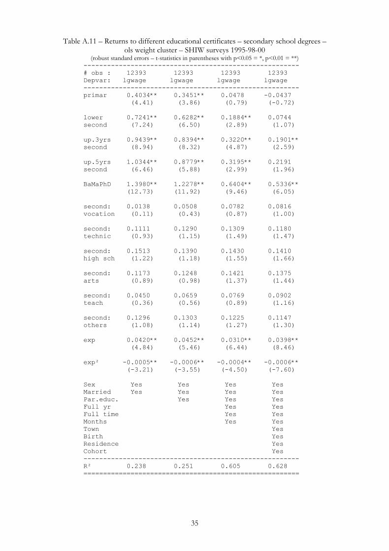
35

Table A.11 – Returns to different educational certificates – secondary school degrees – ols weight cluster – SHIW surveys 1995-98-00

(robust standard errors – t-statistics in parentheses with p<0.05 = *, p<0.01 = **) ------------------------------------------------------- # obs : 12393 12393 12393 12393 Depvar: lgwage lgwage lgwage lgwage ------------------------------------------------------- primar 0.4034** 0.3451** 0.0478 -0.0437 (4.41) (3.86) (0.79) (-0.72) lower 0.7241** 0.6282** 0.1884** 0.0744 second (7.24) (6.50) (2.89) (1.07) up.3yrs 0.9439** 0.8394** 0.3220** 0.1901** second (8.94) (8.32) (4.87) (2.59) up.5yrs 1.0344** 0.8779** 0.3195** 0.2191 second (6.46) (5.88) (2.99) (1.96) BaMaPhD 1.3980** 1.2278** 0.6404** 0.5336** (12.73) (11.92) (9.46) (6.05) second: 0.0138 0.0508 0.0782 0.0816 vocation (0.11) (0.43) (0.87) (1.00) second: 0.1111 0.1290 0.1309 0.1180 technic (0.93) (1.15) (1.49) (1.47) second: 0.1513 0.1390 0.1430 0.1410 high sch (1.22) (1.18) (1.55) (1.66) second: 0.1173 0.1248 0.1421 0.1375 arts (0.89) (0.98) (1.37) (1.44) second: 0.0450 0.0659 0.0769 0.0902 teach (0.36) (0.56) (0.89) (1.16) second: 0.1296 0.1303 0.1225 0.1147 others (1.08) (1.14) (1.27) (1.30) exp 0.0420** 0.0452** 0.0310** 0.0398** (4.84) (5.46) (6.44) (8.46) exp² -0.0005** -0.0006** -0.0004** -0.0006** (-3.21) (-3.55) (-4.50) (-7.60) Sex Yes Yes Yes Yes Married Yes Yes Yes Yes Par.educ. Yes Yes Yes Full yr Yes Yes Full time Yes Yes Months Yes Yes Town Yes Birth Yes Residence Yes Cohort Yes ------------------------------------------------------- R² 0.238 0.251 0.605 0.628 =======================================================

36

Table A.12 – Maximum likelihood probability estimation of labour market participation and employability - weight cluster – SHIW surveys 1993-95-98-00

(robust standard errors – z-statistics in parentheses with p<0.05 = *, p<0.01 = **) ------------------------------------------------------- # obs : 24542 24542 17722 17722 Depvar: lf lf emp emp ------------------------------------------------------- primar 0.1740 0.0618 0.4775** 0.2550 (1.59) (0.48) (2.61) (1.31) lower 0.6626** 0.3355* 0.6429** 0.5368** second (6.00) (2.46) (3.52) (2.71) up.3yrs 0.9748** 0.6243** 0.8782** 0.6704** second (8.58) (4.59) (4.42) (3.11) up.5yrs 3.0520** 2.6915** 0.3784 0.3098 second (7.82) (6.48) (0.91) (0.73) BaMaPhD 1.5410** 1.2496** 0.7650** 0.7338** (10.66) (7.22) (3.58) (3.18) second: -1.9234** -1.9045** 0.6000 0.6475 vocation (-5.00) (-4.80) (1.66) (1.79) second: -1.9026** -1.8864** 0.6575 0.6640 technic (-5.02) (-4.79) (1.86) (1.84) second: -2.5570** -2.5796** 0.2085 0.1812 high sch (-6.63) (-6.46) (0.59) (0.49) second: -2.0646** -1.9904** 0.3490 0.3867 arts (-4.95) (-4.61) (0.93) (1.03) second: -1.8651** -1.7620** 0.2616 0.3573 teach (-5.02) (-4.60) (0.74) (0.93) second: -1.5766** -1.5633** 0.7460 0.7776 others (-3.83) (-3.64) (1.84) (1.77) Sex Yes Yes Yes Yes Married Yes Yes Yes Yes Par.educ. Yes Yes Yes Yes Town Yes Yes Birth Yes Yes Residence Yes Yes Cohort Yes Yes ------------------------------------------------------- PseudoR² 0.237 0.281 0.100 0.194 =======================================================

37

Table A.13 – Expenditure per student by educational level (1999) – relative to GDP per capita pre-primary

education primary

education all secondary

education all tertiary education

France 17 18 31 34 Germany 20 16 27 42 Italy 21 22 27 32 Japan 13 21 24 41 United Kingdom 27 16 24 41 United States 20 20 24 57 OECD average 18 19 25 44

Source: OECD 2002a, table B1.2

Table A.14 – Determinant of years of education – individuals born between 1940 and 1970 - ols weight cluster – SHIW surveys 1993-1995-1998-2000

(robust standard errors – t-statistics in parentheses with p<0.05 = *, p<0.01 = **) ------------------------------------------------------------------------------------------- Model : g1 g2 g3 g4 g5 g6 g7 # obs : 32884 32884 32884 28498 32884 32884 25649 Depvar: edyear edyear edyear edyear edyear edyear edyear ------------------------------------------------------------------------------------------- resources -0.1106** -0.0030 -0.0730** -2.6053 -0.0989 -0.1338** -5.660 (-5.64) (-1.89) (-5.38) (-1.03) (-0.67) (-3.26) (-1.42) parental 0.2502** 0.5108** 0.2625** 0.4134** 0.4530** 0.2978* 0.3827** education (6.81) (12.55) (6.08) (9.56) (26.55) (2.09) (16.89) resour× 0.0120** 0.0000 0.0092** 0.3452 0.0559** 0.0078 1.1019** par.educ. (6.57) (-0.24) (5.43) (1.91) (3.27) (1.40) (4.65) Gender Yes Yes Yes Yes Yes Yes Yes Cohort Yes Yes Yes Yes Yes Yes Yes Birth Yes Yes Yes Yes Yes Yes Yes Residence Yes Yes Yes Yes Yes Yes Yes ------------------------------------------------------------------------------------------- R² 0.331 0.328 0.331 0.31 0.329 0.329 0.312 ===========================================================================================

38

Table A.15 – Maximum likelihood multinomial logit for youngsters’ condition weight cluster – SHIW surveys 1993-95-98-00 –

(relative risk ratios - robust standard errors – z-statistics in parentheses with p<0.05 = *, p<0.01 = **) Individuals coded as “child” or “relative” - “out of labour force” as comparison case

-------------------------------------------------------------- Age: 15 16 17 18 19 # obs : 1171 1113 1199 1270 1347 -------------------------------------------------------------- in school 88.8 83.4 76.8 71.5 55.4 lab.force 9.1 15.1 20.3 25.5 40.4 out lb.frc 2.1 1.5 2.8 3.0 4.2 --------------------------------------------------------------

in school female 0.243* 0.021** 0.003** 0.625 2.788** (-1.82) (-3.41) (-4.90) (-0.85) (2.30) log.fam 1.977* 1.103 0.991 0.654 1.269 income (1.84) (0.35) (-0.02) (-1.11) (1.07) father 1.3e+9** 4.017 4.3e+10** 11.28** 1.943 up.secnd (24.68) (1.14) (78.9) (2.11) (1.69) father 0.030 0.045** 1.8e+13** 7.488 9.8e+8** college (-1.65) (-5.95) (29.6) (1.74) (29.4) mother 200.0** 199.3** 9.995 2.1e+9** 6.128* up.secnd (2.38) (7.34) (1.31) (43.3) (1.95) mother 646.8** 4.1e+16** 0.004** 7.942 7.6e+9** college (2.92) (42.2) (-4.05) (1.72) (22.0)

employed/unemployed/first job seeker female 0.158** 0.011** 0.002** 0.365 2.081 (-2.24) (-3.55) (-5.32) (-1.53) (1.48) log.fam 1.562 0.958 0.807 0.573 1.209 income (1.68)* (-0.10) (-0.55) (-1.19) (1.03) father 7.4e+7 0.359 8.3e+9 2.7e+8 0.406** up.secnd --- (-0.81) --- (0.34) (-2.37) father 2.8e-7** 0.018** 5.9e+11 0.140 1.4e+8 college (-20.1) (-3.65) --- (0.04) --- mother 13.01 5.839** 1.540 2.7e+8 0.713 up.secnd (1.04) (2.27) (0.25) --- (-0.37) mother 9.9e-13** 69.60** 0.000** 0.140 1.5e+8 college (-12.4) (5.15) (-5.27) (-1.07) --- -------------------------------------------------------------- pseudoR² 0.326 0.296 0.281 0.200 0.184 ============================================================== Note: macro-region of residence and town size are included as additional regressors in all specifications.

39

Table A.16 – Maximum likelihood probit estimation of university attendance weight cluster – SHIW surveys 1995-98-00 – marginal effects

(robust standard errors – z-statistics in parentheses with p<0.05 = *, p<0.01 = **) Individuals coded as “child” or “relative”, with a secondary school degree

------------------------------------------------------------------------------- Age: 19 19 20 20 21 21 # obs : 541 541 696 696 709 709 Depvar: uni uni uni uni uni uni ------------------------------------------------------------------------------- un.student 30.1 30.1 41.3 41.3 48.8 48.8 not studnt 69.9 69.9 58.7 58.7 51.2 51.2 ------------------------------------------------------------------------------- female -0.174 -0.090 -0.079* 0.066 0.074 -0.021 (-0.23) (-1.34) (2.49) (1.21) (1.57) (-0.44) log.eq. -0.003 -0.047 -0.036 -0.051 -0.017 -0.090 fam.incm (-0.06) (-0.89) (-0.85) (-1.23) (-0.41) (-1.70) father 0.067 -0.025 0.010 0.006 0.226** 0.205** up.secnd (1.07) (-0.41) (0.12) (0.06) (3.15) (2.81) father 0.204 0.052 0.159 0.086 0.374** 0.313** college (1.65) (0.36) (1.27) (0.63) (3.89) (3.37) mother 0.289** 0.200* 0.280** 0.231* 0.422** 0.357* up.secnd (3.20) (1.78) (2.76) (2.21) (2.98) (2.41) mother 1.000** 1.000** 0.406** 0.357** 0.502** 0.451** college (0.0) (0.0) (5.22) (3.45) (4.09) (3.40) vocational 0.148 0.032 -0.072** up.second (1.29) (0.21) (-0.61) technical 0.146 0.209* 0.170** up.second (1.39) (1.92) (2.73) high school 0.411** 0.505** 0.627** (6.93) (4.36) (5.28) Town Yes Yes Yes Yes Yes Yes Area Yes Yes Yes Yes Yes Yes ------------------------------------------------------------------------------- R² 0.108 0.191 0.118 0.235 0.131 0.304 ===============================================================================

40

Table A.17 – Descriptive statistics – Italian students exiting secondary school in 1995 (weighed) standard deviation in brackets

Number of observations 18.843 Gender 52.41 Age 19.82 (2.72) Judgment obtained at exit of lower secondary school (%): sufficient (sufficiente) 33.27 good (buono) 27.71 very good (distinto) 20.03 excellent (ottimo) 18.99 Marks obtained at exit of upper secondary school (over 60) 45.02 (6.96) Secondary school attendance (%): vocational school (istituti tecnici professionali) 14.63 technical school (istituti tecnici) 45.54 teaching school (istituti magistrali) 8.24 high school (licei classici, scientifici, linguistici) 28.26 school of arts (istituti artistici) 3.32

41

Table A.18 – Maximum likelihood probit estimation of university attendance weight cluster – ISTAT survey 1995 – marginal effects

(robust standard errors – z-statistics in parentheses with p<0.05 = *, p<0.01 = **)

------------------------------- # obs : 17418 17418 Depvar: uni uni ------------------------------- un.student 50.2 50.2 not studnt 49.8 49.8 ------------------------------- female -0.015 -0.015 (-0.95) (-0.94) age -0.017** -0.017** (-3.56) (-3.47) jdg.exit 0.036** 0.036** lw.secnd (3.55) (3.77) mrk.exit 0.022** 0.022** up.secnd (21.73) (21.97) vocation. -0.105** -0.105** school (-3.45) (-3.53) technical 0.093** 0.092** school (4.20) (4.08) teaching 0.212** 0.213** school (7.41) (6.76) high 0.548** 0.549** school (17.77) (17.74) parent -0.003 -0.003 primary (-0.06) (-0.07) parent 0.056 0.055 lw.secnd (1.24) (1.19) parent 0.115* 0.115* 3-yr scnd (2.35) (2.24) parent 0.179** 0.179** 5-yr scnd (3.96) (3.85) parent 0.192* 0.192* tert.deg (2.19) (2.14) parent 0.305** 0.306** BA-MA-PhD (6.87) (6.79) private -0.004 (-0.13) Region Yes Yes ------------------------------- R-sq 0.334 0.334 ===============================

42

Figure A.1 – Return to education and union presence es

timat

ed re

turn

to a

dd.y

ear o

f edu

catio

n - m

en

union density 1994-96

ed.return men Fitted values

0 .5 1

.04

.06

.08

.1

France

Spain

Switzerl

Netherla

WestGerm

GreatBri

Italy

Portugal

Austria

Ireland

Norway

Denmark

Finland

Sweden

43

Figure A.2 - Current status by age and macro area of residence – Italy 1993-95-98-2000 pe

rcen

t

Northage

0

.2

.4

.6

.8

1

in school seeking a job unemployed employed out of labour force

11 12 13 14 15 16 17 18 19 20 21 22 23 24 25 26 27 28 29 30

perc

ent

Centreage

0

.2

.4

.6

.8

1

in school seeking a job unemployed employed out of labour force

11 12 13 14 15 16 17 18 19 20 21 22 23 24 25 26 27 28 29 30

perc

ent

Southage

0

.2

.4

.6

.8

1

in school seeking a job unemployed employed out of labour force

11 12 13 14 15 16 17 18 19 20 21 22 23 24 25 26 27 28 29 30

perc

ent

Islandsage

0

.2

.4

.6

.8

1

in school seeking a job unemployed employed out of labour force

11 12 13 14 15 16 17 18 19 20 21 22 23 24 25 26 27 28 29 30

44

Figure A.3 – Average number of children in families by average age of children – Italy 1993-95-98-2000

average age children

+ 1 st.dev. average num.children - 1 st.dev.

10 15 20 25 30

0

1

2

3

4