The Journal of FOUNDATIONS CIENCEcommonsensescience.net/pdf/articles/v20n2_The_Experimental... · electrodynamics known as Gauss’s Electrostatic and Magnetostatic Laws, Ampere’s

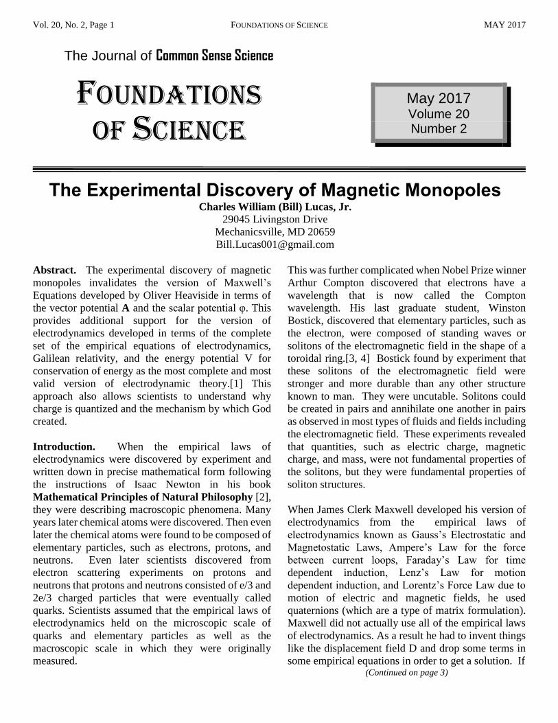
Vol. 20, No. 2, Page 1 FOUNDATIONS OF SCIENCE MAY 2017

Abstract. The experimental discovery of magnetic

monopoles invalidates the version of Maxwell’s

Equations developed by Oliver Heaviside in terms of

the vector potential A and the scalar potential φ. This

provides additional support for the version of

electrodynamics developed in terms of the complete

set of the empirical equations of electrodynamics,

Galilean relativity, and the energy potential V for

conservation of energy as the most complete and most

valid version of electrodynamic theory.[1] This

approach also allows scientists to understand why

charge is quantized and the mechanism by which God

created.

Introduction. When the empirical laws of

electrodynamics were discovered by experiment and

written down in precise mathematical form following

the instructions of Isaac Newton in his book

Mathematical Principles of Natural Philosophy [2],

they were describing macroscopic phenomena. Many

years later chemical atoms were discovered. Then even

later the chemical atoms were found to be composed of

elementary particles, such as electrons, protons, and

neutrons. Even later scientists discovered from

electron scattering experiments on protons and

neutrons that protons and neutrons consisted of e/3 and

2e/3 charged particles that were eventually called

quarks. Scientists assumed that the empirical laws of

electrodynamics held on the microscopic scale of

quarks and elementary particles as well as the

macroscopic scale in which they were originally

measured.

This was further complicated when Nobel Prize winner

Arthur Compton discovered that electrons have a

wavelength that is now called the Compton

wavelength. His last graduate student, Winston

Bostick, discovered that elementary particles, such as

the electron, were composed of standing waves or

solitons of the electromagnetic field in the shape of a

toroidal ring.[3, 4] Bostick found by experiment that

these solitons of the electromagnetic field were

stronger and more durable than any other structure

known to man. They were uncutable. Solitons could

be created in pairs and annihilate one another in pairs

as observed in most types of fluids and fields including

the electromagnetic field. These experiments revealed

that quantities, such as electric charge, magnetic

charge, and mass, were not fundamental properties of

the solitons, but they were fundamental properties of

soliton structures.

When James Clerk Maxwell developed his version of

electrodynamics from the empirical laws of

electrodynamics known as Gauss’s Electrostatic and

Magnetostatic Laws, Ampere’s Law for the force

between current loops, Faraday’s Law for time

dependent induction, Lenz’s Law for motion

dependent induction, and Lorentz’s Force Law due to

motion of electric and magnetic fields, he used

quaternions (which are a type of matrix formulation).

Maxwell did not actually use all of the empirical laws

of electrodynamics. As a result he had to invent things

like the displacement field D and drop some terms in

some empirical equations in order to get a solution. If (Continued on page 3)

May 2017

Volume 20 Number 2

The Experimental Discovery of Magnetic Monopoles Charles William (Bill) Lucas, Jr.

29045 Livingston Drive

Mechanicsville, MD 20659

[email protected]

The Journal of Common Sense Science

FOUNDATIONS OF SCIENCE



© 2017, Common Sense Science, Inc.

Published 4 times each year by

Common Sense Science, Inc.,

Charles William (Bill) Lucas Jr, Editor,

Glen C. Collins, Assistant Editor.

Internet: www.CommonSenseScience.org

Email: [email protected]

Telephone: 1-240-249-5589

Subscription Rates (four issues)

Science Partner Subscription: US $100

Regular Subscription by mail: US $25

Senior Subscription by mail: US $15

Regular Subscription by email; US $15

Student Subscription by email: US $10

Free subscription by email: Free for 1 year

Send request for subscription or address change to:

Common Sense Science, Inc.

29045 Livingston Drive

Mechanicsville, Maryland 29045-3271 USA

or [email protected]

DONATIONS: Common Sense Science is a non-profit organization

incorporated by the State of Georgia and recognized by the IRS

as a tax-exempt 501(c) (3) organization. Gifts to Common Sense

Science are tax deductible.

SENDING FUNDS: You may mail a check (payable in U. S.

dollars) to Common Sense Science, or you may use a credit card

to transmit funds by PayPal at the CSS website.

CORRESPONDENCE: Send editorial correspondence to Common

Sense Science at address above. FOUNDATIONS OF SCIENCE is

not a journal to review & publish just anyone’s scientific papers.

DIRECTORS of Common Sense Science:

David L. Bergman, President, Treasurer

Charles W. (Bill) Lucas, Jr., President

David L. Bergman - Director

Glen C. Collins, Director


Mailed This Issue:

Within US – 145

Outside US – 21

Email – 5

Letters and E-Mail Correspondence

Special Notices

The Directors and some loyal supporters of

Common Sense Science held an on-line

meeting at 10:00 AM EST on February 21,

2017. At that meeting David Bergman resigned

as President and Bill Lucas was elected as the

new President and Treasurer. Dave is still a

Director on the Board of Directors.

In the next few months an effort will be made

to establish a list of leaders at each of the major

scientific institutions in the United States. The

list will consist of contact name, position,

institution, postal address, email address and

telephone number. Each leader will also be

given a code to identify their interest as only

science or also the Judeo-Christian religious

aspects of science. We will also be creating a

list of leaders with a special religious code at

the Judeo-Christian seminaries, Bible colleges,

and universities. Once these lists are

established we will begin regular emails to the

various codes with information about the

reformation in science that we are attempting

to lead on a regular basis. All feedback from

these contacts will be welcome. If you are

interested in helping us develop our contact

lists, speaking engagements with scientific

organizations, colleges and universities and

Judeo-Christian seminaries and Bible schools,

please contact [email protected].

Back Issues are Available

Back Issues of FOUNDATIONS OF SCIENCE are

available to the general public online for free at

www.commonsensescience.org


The Experimental Discovery of Magnetic

Monopoles (Continued from page 1)

Maxwell had used all six of the empirical equations of

electrodynamics plus Galilean Relativity and

conservation of energy, he would not have had to

arbitrarily invent the displacement field and drop some

terms in order to get a solution. Despite these

irregularities, Maxwell was able to combine four of the

six laws of electricity and magnetism together into

electrodynamics and explain the wave nature of light

as the foundation of optics. This was considered great

progress in his day.

One of Maxwell’s followers, Oliver Heaviside, found

that the quaternion matrix approach of Maxwell was

too complicated and difficult for scientists of his day

to use. So he redid Maxwell’s quaternion equations in

terms of vectors. This is the version that is still used

today and called Maxwell’s Equations.

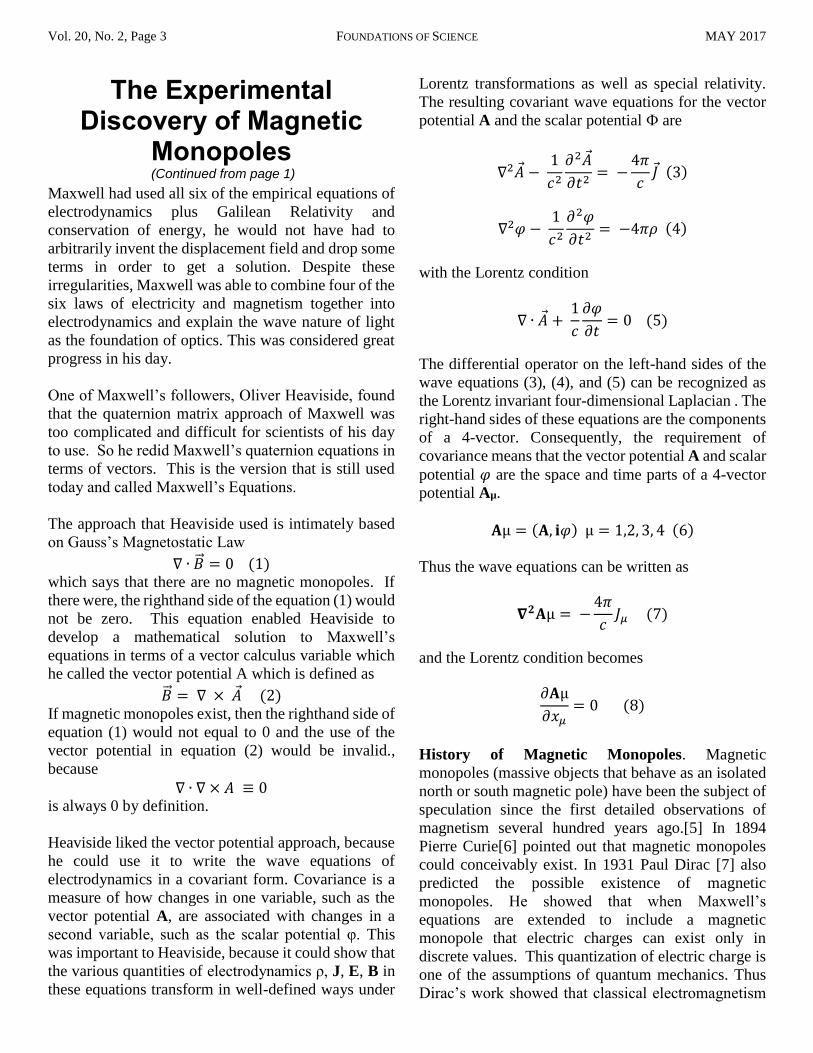
The approach that Heaviside used is intimately based

on Gauss’s Magnetostatic Law

∇ ∙ �⃗� = 0 (1) which says that there are no magnetic monopoles. If

there were, the righthand side of the equation (1) would

not be zero. This equation enabled Heaviside to

develop a mathematical solution to Maxwell’s

equations in terms of a vector calculus variable which

he called the vector potential A which is defined as

�⃗� = ∇ × 𝐴 (2)

If magnetic monopoles exist, then the righthand side of

equation (1) would not equal to 0 and the use of the

vector potential in equation (2) would be invalid.,

because

∇ ∙ ∇ × 𝐴 ≡ 0 is always 0 by definition.

Heaviside liked the vector potential approach, because

he could use it to write the wave equations of

electrodynamics in a covariant form. Covariance is a

measure of how changes in one variable, such as the

vector potential A, are associated with changes in a

second variable, such as the scalar potential φ. This

was important to Heaviside, because it could show that

the various quantities of electrodynamics ρ, J, E, B in

these equations transform in well-defined ways under

Lorentz transformations as well as special relativity.

The resulting covariant wave equations for the vector

potential A and the scalar potential Փ are

∇2𝐴 − 1

𝑐2

𝜕2𝐴

𝜕𝑡2= −

4𝜋

𝑐𝐽 (3)

∇2𝜑 − 1

𝑐2

𝜕2𝜑

𝜕𝑡2= −4𝜋𝜌 (4)

with the Lorentz condition

∇ ∙ 𝐴 + 1

𝑐

𝜕𝜑

𝜕𝑡= 0 (5)

The differential operator on the left-hand sides of the

wave equations (3), (4), and (5) can be recognized as

the Lorentz invariant four-dimensional Laplacian . The

right-hand sides of these equations are the components

of a 4-vector. Consequently, the requirement of

covariance means that the vector potential A and scalar

potential 𝜑 are the space and time parts of a 4-vector

potential Aµ.

𝐀µ = (𝐀, 𝐢𝜑) µ = 1,2, 3, 4 (6)

Thus the wave equations can be written as

𝛁𝟐𝐀µ = −4𝜋

𝑐𝐽𝜇 (7)

and the Lorentz condition becomes

𝜕𝐀µ

𝜕𝑥𝜇= 0 (8)

History of Magnetic Monopoles. Magnetic

monopoles (massive objects that behave as an isolated

north or south magnetic pole) have been the subject of

speculation since the first detailed observations of

magnetism several hundred years ago.[5] In 1894

Pierre Curie[6] pointed out that magnetic monopoles

could conceivably exist. In 1931 Paul Dirac [7] also

predicted the possible existence of magnetic

monopoles. He showed that when Maxwell’s

equations are extended to include a magnetic

monopole that electric charges can exist only in

discrete values. This quantization of electric charge is

one of the assumptions of quantum mechanics. Thus

Dirac’s work showed that classical electromagnetism


and quantum mechanics could be compatible theories

based on quantization of charge if magnetic monopoles

exist.

Numerous theoretical investigations and hitherto

unsuccessful experimental searches[8] have followed

Dirac’s 1931 development of a theory of monopoles

consistent with both quantum mechanics and the gauge

invariance of the electromagnetic field.[7] The

existence of even a single Dirac magnetic monopole

would have far-reaching consequences including an

explanation for the quantization of electric charge.[7,

8] Gauge theory is a type of field theory in which the

Lagrangian is invariant under a continuous group of

local transformations.

Many scientists believe that nature is symmetric. The

existence of magnetic monopoles would imply a

duality between electricity and magnetism. Maxwell’s

equations could be written in a symmetric fashion such

that the role of the electric and magnetic fields would

become more fundamental than the role of the non-

physical vector potential A and the scalar potential φ.

This is shown in equations (9), (10), (11), (12), and

(13).

Gauss′s electrostatic law ∇ ∙ 𝐸 = 4𝜋𝜌𝑒 (9)

Gauss′s magnetostatic law ∇ ∙ 𝐵 = 4𝜋𝜌𝑚 (10)

Faraday′s law − ∇ × 𝐸 = 1

𝑐

𝜕𝐵

𝜕𝑡 +

4𝜋

𝑐 𝑗𝑚 (11)

Ampere′s law ∇ × 𝐵 = 1

𝑐 𝜕𝐸

𝜕𝑡+

4𝜋

𝑐𝑗𝑒 (12)

Lorentz′s force law

𝐹 = 𝑞𝑒 (𝐸 + 𝑣

𝑐× 𝐵) + 𝑞𝑚 (𝐵 −

𝑣

𝑐× 𝐸) (13)

Although analogues of magnetic monopoles have been

found in exotic spin ices[10, 11] and other systems[12,

13, 14], there had been no direct experimental

observation of Dirac monopoles within a medium

described by a quantum field, such as superfluid

helium-3.[15, 16, 17, 18] Then in 2014 Dirac

monopoles were finally observed in a synthetic

magnetic field produced by a spinor Bose-Einstein

condensate.[19]

As a result of this work an international collaboration

was set up at Amherst College by Physics Professor

David S Hall and Aalto University (Finland) Academy

Research Fellow Mikko Mottonen. They have

identified and photographed synthetic magnetic

monopoles in Hall’s laboratory on the Amherst

campus.[20]

Monopoles are identified, in both experiments and

matching numerical simulations, at the termini of

vortex lines within the condensate. By directly

imaging such vortex lines, the presence of a monopole

may be discerned from the experimental data alone.

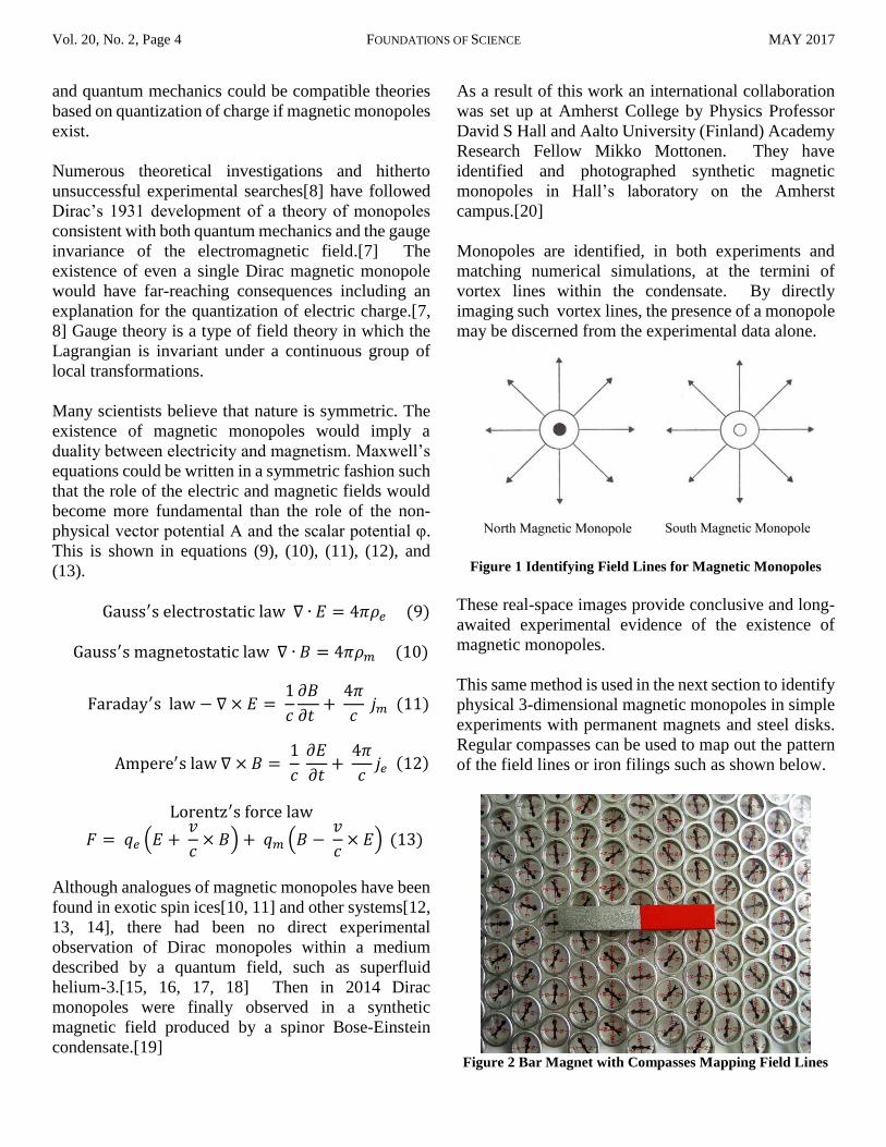
Figure 1 Identifying Field Lines for Magnetic Monopoles

These real-space images provide conclusive and long-

awaited experimental evidence of the existence of

magnetic monopoles.

This same method is used in the next section to identify

physical 3-dimensional magnetic monopoles in simple

experiments with permanent magnets and steel disks.

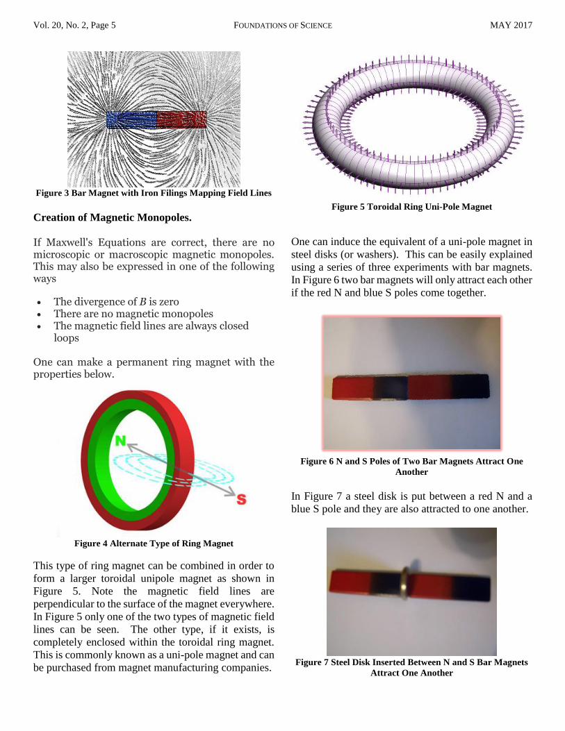
Regular compasses can be used to map out the pattern

of the field lines or iron filings such as shown below.

Figure 2 Bar Magnet with Compasses Mapping Field Lines


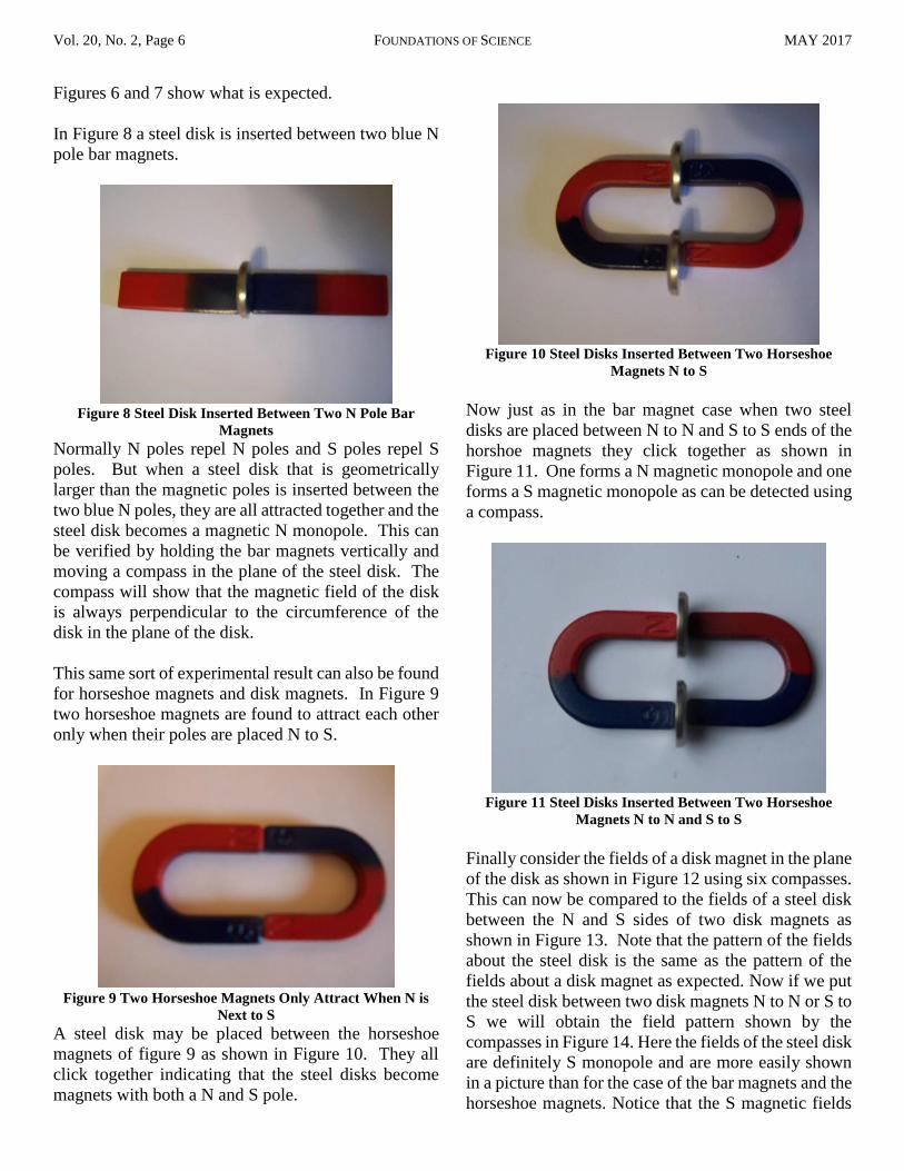
Figure 3 Bar Magnet with Iron Filings Mapping Field Lines

Creation of Magnetic Monopoles.

If Maxwell's Equations are correct, there are no microscopic or macroscopic magnetic monopoles. This may also be expressed in one of the following ways

The divergence of B is zero There are no magnetic monopoles The magnetic field lines are always closed

loops

One can make a permanent ring magnet with the properties below.

Figure 4 Alternate Type of Ring Magnet

This type of ring magnet can be combined in order to

form a larger toroidal unipole magnet as shown in

Figure 5. Note the magnetic field lines are

perpendicular to the surface of the magnet everywhere.

In Figure 5 only one of the two types of magnetic field

lines can be seen. The other type, if it exists, is

completely enclosed within the toroidal ring magnet.

This is commonly known as a uni-pole magnet and can

be purchased from magnet manufacturing companies.

Figure 5 Toroidal Ring Uni-Pole Magnet

One can induce the equivalent of a uni-pole magnet in

steel disks (or washers). This can be easily explained

using a series of three experiments with bar magnets.

In Figure 6 two bar magnets will only attract each other

if the red N and blue S poles come together.

Figure 6 N and S Poles of Two Bar Magnets Attract One

Another

In Figure 7 a steel disk is put between a red N and a

blue S pole and they are also attracted to one another.

Figure 7 Steel Disk Inserted Between N and S Bar Magnets

Attract One Another


Figures 6 and 7 show what is expected.

In Figure 8 a steel disk is inserted between two blue N

pole bar magnets.

Figure 8 Steel Disk Inserted Between Two N Pole Bar

Magnets Normally N poles repel N poles and S poles repel S

poles. But when a steel disk that is geometrically

larger than the magnetic poles is inserted between the

two blue N poles, they are all attracted together and the

steel disk becomes a magnetic N monopole. This can

be verified by holding the bar magnets vertically and

moving a compass in the plane of the steel disk. The

compass will show that the magnetic field of the disk

is always perpendicular to the circumference of the

disk in the plane of the disk.

This same sort of experimental result can also be found

for horseshoe magnets and disk magnets. In Figure 9

two horseshoe magnets are found to attract each other

only when their poles are placed N to S.

Figure 9 Two Horseshoe Magnets Only Attract When N is

Next to S A steel disk may be placed between the horseshoe

magnets of figure 9 as shown in Figure 10. They all

click together indicating that the steel disks become

magnets with both a N and S pole.

Figure 10 Steel Disks Inserted Between Two Horseshoe

Magnets N to S

Now just as in the bar magnet case when two steel

disks are placed between N to N and S to S ends of the

horshoe magnets they click together as shown in

Figure 11. One forms a N magnetic monopole and one

forms a S magnetic monopole as can be detected using

a compass.

Figure 11 Steel Disks Inserted Between Two Horseshoe

Magnets N to N and S to S

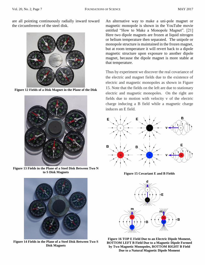
Finally consider the fields of a disk magnet in the plane

of the disk as shown in Figure 12 using six compasses.

This can now be compared to the fields of a steel disk

between the N and S sides of two disk magnets as

shown in Figure 13. Note that the pattern of the fields

about the steel disk is the same as the pattern of the

fields about a disk magnet as expected. Now if we put

the steel disk between two disk magnets N to N or S to

S we will obtain the field pattern shown by the

compasses in Figure 14. Here the fields of the steel disk

are definitely S monopole and are more easily shown

in a picture than for the case of the bar magnets and the

horseshoe magnets. Notice that the S magnetic fields


are all pointing continuously radially inward toward

the circumference of the steel disk.

Figure 12 Fields of a Disk Magnet in the Plane of the Disk

Figure 13 Fields in the Plane of a Steel Disk Between Two N

to S Disk Magnets

Figure 14 Fields in the Plane of a Steel Disk Between Two S

Disk Magnets

An alternative way to make a uni-pole magnet or

magnetic monopole is shown in the YouTube movie

entitled “How to Make a Monopole Magnet”. [21]

Here two dipole magnets are frozen at liquid nitrogen

or helium temperature then separated. The unipole or

monopole structure is maintained in the frozen magnet,

but at room temperature it will revert back to a dipole

magnetic structure upon exposure to another dipole

magnet, because the dipole magnet is more stable at

that temperature.

Thus by experiment we discover the real covariance of

the electric and magnet fields due to the existence of

electric and magnetic monopoles as shown in Figure

15. Note that the fields on the left are due to stationary

electric and magnetic monopoles. On the right are

fields due to motion with velocity v of the electric

charge inducing a B field while a magnetic charge

induces an E field.

Figure 15 Covariant E and B Fields

Figure 16 TOP E Field Due to an Electric Dipole Moment,

BOTTOM LEFT B Field Due to a Magnetic Dipole Formed

by Two Magnetic Monopoles, BOTTOM RIGHT B Field

Due to a Natural Magnetic Dipole Moment


In Figure 16 note that the electric and magnetic dipole

fields are more identical or covariant when magnetic

monopoles are used instead of magnetic dipoles.

Conclusions. The discovery that the external magnetic

fields of a magnet depend on the geometry of the

magnet enabled scientists to create magnetic

monopoles for certain geometries. Thus Gauss’s law

for magnetism needs to be changed to allow for

monopole and unipole type magnetic geometries. This

change invalidates the vector potential approach to

solving Maxwell’s equations. Instead of the

covariance of electrodynamics being expressed in

terms of the vector and scaler potential, the covariance

can now be expressed more naturally in terms of the

electric E and magnetic B fields. This implies that the

electromagnetic E and B fields are more fundamental

than the non-physical vector potential A and scalar

potential φ. It allows the use of the energy potential V

approach[1] enabling the conservation of energy in

electrodynamics. The vector potential approach to

solving Maxwell’s equations does not conserve energy

explicitly.

Before the discovery of magnetic monopoles or uni-

poles there were three basic approaches to

electrodynamics. The first approach was due to

Weber[22] and was based on Coulomb’s law for the

force between static charges, Ampere’s law for the

force between current elements, Faraday’s law of

electromagnetic induction, Newton’s third law and

conservation of energy. [24] The second was due to

Oliver Heaviside’s vector version of Maxwell’s

equations using 4 of the 6 empirical equations of

electrodynamics and solving them in terms of the

vector and scalar potentials with no conservation of

energy or magnetic monopoles. The third was due to

the author’s[1] use of the complete set of the empirical

equations of electrodynamics which includes Lenz’s

Law, Galilean relativity, and conservation of energy.

After the discovery of magnetic monopoles the

author’s approach is left as the only standing and the

only complete description of electrodynamics.

Furthermore the energy potential approach enables a

more general solution of the empirical equations of

electrodynamics that includes the acceleration a terms

describing radiation emission and absorption plus the

radiation recoil or reaction da/dt terms. These terms

are missing from Weber’s approach, Maxwell’s

Equations and even special relativity making the vector

potential approach to solving Maxwell’s equations and

combining them with special relativity incomplete.

Besides the energy potential approach[1] gives all the

special relativistic type factors like

𝛾 = 1

√1 − 𝑣2

𝑐2⁄

(10)

directly from Lenz’s Law and Galilean relativity

without any reference to special relativity at all.

Applying special relativity to the energy potential

version of electrodynamics would be redundant,

illogical and totally unnecessary!! Also note that

many of the assumptions of special relativity are

known by experiment to be false. For example special

relativity assumes that space is homogeneous and

isotropic with no center, but astronomical observations

show that the universe is not homogeneous and

isotropic, since solar systems, galaxies, and shells of

galaxies have a center.

Finally requiring the author’s version of

electrodynamics[1] with its three radiation reaction

da/dt terms to be in agreement with experiment,

appears to be satisfied only if the boundary condition

that all electromagnetic structures in nature are

composed of toroidal ring solitons of the

electromagnetic field in agreement with the work of

Arthur Compton, Winston Bostick[3,4], and Dave

Bergman[23] is true.

In the toroidal loop of the soliton the standing waves

dpend on the amount of magnetic flux in the loop. The

wave must have the same value after each revolution

around the loop that it had at the start for coherence

and stability. Only special values of the

electromagnetic field wave flux let that happen. Those


values are zero or some integer multiple of the

minimum flux for a standing wave in the toroidal ring.

What makes electrical charge (equivalent to the

electrical flux leaving a particle) to be quantized? In

the past Dirac [7] argued that if there are magnetic

monopoles, they too must have well defined quantum

states. This requirement places a constraint on electron

fluxes. That constraint leads to the requirement that

electrical charge be quantized in agreement with this

paper based on the author’s development of

electrodynamics.

Electron scattering experiments on protons and

neutrons have found that protons and neutrons are

composed of three sub-particles called quarks with

charges of ± e/3 and ± 2e/3 where e is the charge of the

electron. Thus from these experiments the minimum

quantum of charge is ± e/3 suggesting that the electron

consists of at least three toroidal rings of charge e/3.

Finally the discovery of magnetic monopoles and the

discrediting of Weber’s approach to electrodynamics

as well as Maxwell’s and Oliver Heaviside’s approach

leaves only one valid approach.[1] This approach,

which uses all the empirical equations of

electrodynamics plus Galilean relativity and

conservation of energy, explains electrodynamics

better than any previous approach and it explains how

God created the universe and maintains it.[25]

According to this approach to electrodynamics[1] all

particles of matter in the universe are composed of

standing wave solitons of the electromagnetic field.

The Bible identifies God as the source of the

electromagnetic field from which all matter is made

from rays of light forming solitons in the field.

And God said, “Let there be light,” and there was

light. [Genesis 1:3 KJV]

His brightness was like the light; He had rays

flashing from His hand, And there His power was

hidden. [Habakkuk 3:4 NKJV]

Furthermore the spherical and chiral symmetry of all

the terms of the electrodynamic force is in perfect

agreement with the structure or symmetry of the

Godhead of the Bible which produces it.

For since the creation of the world His invisible

attributes are clearly seen, being understood by the

things that He made, even His eternal power and

the structure of the Godhead, so mankind is

without excuse [Romans 1:20 NKJV]

The symmetry of God and the electrodynamic force are

seen in the symmetry of all known elementary

particles, atoms, nuclei, crystals, plant leaves, plant

flowers, animal body structures, orbits of the planets

about the sun, orbits of the moons about the planets,

the structure of the Milky Way galaxy, and the overall

structure of the universe about its center.[25]

References.

1. Charles W. Lucas, Jr., The Universal Force

Volume 1 – Derived From A More Perfect

Union of the Axiomatic and Empirical

Scientific Methods, (Create Space, May

2013). See www.amazon.com

2. Isaac Newton, The Principia, Mathematical

Principles of Natural Philosophy: A New

Translation, translators I Bernard Cohen and

Anne Whitman (University of California Press,

Berkeley, 1999).

3. Bostick, Winston H., W. Prior, L. Grunberger,

and G. Emmert, "Pair Production of Plasma

Vortices", Physics of Fluids, Vol. 9, Issue 10,

pp. 2078-2080 (1966).

4. Bostick, Winston H., “Mass, Charge, and

Current: The Essence and Morphology,”

Physics Essays, Vol. 4, No. 1, pp. 45-59

(1991).

5. A. S. Goldhaber, W. P. Trower, editors

Magnetic Monopoles (American Association

of Physics Teachers), 1990.

6. Pierre Curie, “Sur la possibilité d'existence de

la conductibilité magnétique et du magnétisme

libre” (On the possible existence of magnetic


conductivity and free magnetism), Séances de

la Société Française de Physique (Paris), p76

(1894).

7. Paul Dirac, “Quantized Singularities in the

Electromagnetic Field”, Proc. Roy. Soc.

(London) A 133, pp 60-72 (1931).

8. Milton, K. A. “Theoretical and Experimental

Status of Magnetic Monopoles”, Rep. Prog.

Phys. 69, pp. 1637–1711 (2006).

9. Vilenkin A., Shellard E. P. S., eds. Cosmic

Strings and Other Topological

Defects (Cambridge Univ. Press, 1994).

10. Castelnovo, C., Moessner, R. & Sondhi, S.

L., “Magnetic Monopoles in Spin

Ice”, Nature 451, pp 42–45 (2008).

11. Morris, D. J. P. et al. “Dirac Strings and

Magnetic Monopoles in the Spin Ice

Dy2Ti2O7”, Science 326, 411–414 (2009).

12. Chuang, I., Durrer, R., Turok, N. & Yurke,

B. “Cosmology in the Laboratory: Defect

Dynamics in Liquid Crystals”, Science 251, pp

1336–1342 (1991).

13. Fang, Z. et al. “The Anomalous Hall Effect and

Magnetic Monopoles in Momentum

Space” Science 302, pp. 92–95 (2003).

14. Milde, P. et al. “Unwinding of a Skyrmion

Lattice By Magnetic Monopoles”,

Science 340, pp. 1076–1080 (2013).

15. Blaha, S., “Quantization Rules for Point

Singularities in Superfluid 3He and Liquid

Crystals”, Phys. Rev. Lett. 36, pp. 874 -

876 (1976)

16. Volovik, G. & Mineev, V. P. “Vortices With

Free Ends in Superfluid He3-A”, JETP

Lett. 23, pp. 647–649 (1976).

17. Salomaa, M. M. “Monopoles in the Rotating

Superfluid Helium-3 A–B

Interface”, Nature 326, pp. 367–370 (1987).

18. Volovik, G. “The Universe in a Helium

Droplet”, (Oxford Univ. Press), pp 214-217

(2003).

19. Pietilä, V. & Möttönen, M. “Creation of Dirac

Monopoles in Spinor Bose-Einstein

Condensates”, Phys. Rev. Lett. , 103, pp.

030401 (2009).

20. M. W. Ray, E. Ruokokoski, S. Kandel, M.

Möttönen, and D. S. Hall, “Observation of

Dirac Monopoles in a Synthetic Magnetic

Field”, Nature 505, pp. 657-660 (2014).

21. How to Make A Monopole Magnet

https://www.youtube.com/watch?v=fn4A6VJo

dow

22. Andre Koch Torres Assis, Weber’s

Electrodynamics (Kluwer Academic

Publishers, Norwell, MA, 1994).

23. D. L. Bergman and J. P. Wesley, “Spinning

Charged Ring Model of Electron Yielding

Anomalous Magnetic Moment,” Galilean

Electrodynamics, vol. 1, no. 5, pp. 63-67

(Sept/Oct, 1990).

24. C. W. Lucas, Jr. and J. C. Lucas, “Weber’s

Force Law for Finite-Size Elastic Particles”,

Galilean Electrodynamics, vol. 14, no. 1, pp.

3-10 (Jan/Feb, 2003).

25. Charles W. Lucas, Jr., Fingerprints of the

Creator – The Source of All Beauty in

Nature, (Create Space, March 2014).See

www.amazon.com

Documents

The Journal of FOUNDATIONS CIENCEcommonsensescience.net/pdf/articles/v20n2_The_Experimental... · electrodynamics known as Gauss’s Electrostatic and Magnetostatic Laws, Ampere’s