Embed Size (px)
Citation preview

The Kappa platform for rule-based modeling
Pierre Boutillier1,*, Mutaamba Maasha1, Xing Li1,2,
Hector F. Medina-Abarca1, Jean Krivine3, Jerome Feret4,
Ioana Cristescu1, Angus G. Forbes5,* and Walter Fontana1,*
1Department of Systems Biology, Harvard Medical School, Boston, MA 02115, USA, 2Edgewise Networks, Burlington,
MA 01803, USA, 3IRIF, Universite Paris-Diderot – Paris 7 F-75205 Paris, France, 4Departement d’informatique
de l’ENS (INRIA/ENS/CNRS), PSL Research University, F-75005 Paris, France and 5Department of Computational
Media, UC Santa Cruz, Santa Cruz, CA 95064, USA
*To whom correspondence should be addressed.
Abstract
Motivation: We present an overview of the Kappa platform, an integrated suite of analysis and
visualization techniques for building and interactively exploring rule-based models. The main compo-
nents of the platform are the Kappa Simulator, the Kappa Static Analyzer and the Kappa Story
Extractor. In addition to these components, we describe the Kappa User Interface, which includes a
range of interactive visualization tools for rule-based models needed to make sense of the complexity
of biological systems. We argue that, in this approach, modeling is akin to programming and can like-
wise benefit from an integrated development environment. Our platform is a step in this direction.
Results: We discuss details about the computation and rendering of static, dynamic, and causal
views of a model, which include the contact map (CM), snaphots at different resolutions, the
dynamic influence network (DIN) and causal compression. We provide use cases illustrating how
these concepts generate insight. Specifically, we show how the CM and snapshots provide infor-
mation about systems capable of polymerization, such as Wnt signaling. A well-understood model
of the KaiABC oscillator, translated into Kappa from the literature, is deployed to demonstrate the
DIN and its use in understanding systems dynamics. Finally, we discuss how pathways might be
discovered or recovered from a rule-based model by means of causal compression, as exemplified
for early events in EGF signaling.
Availability and implementation: The Kappa platform is available via the project website at kappa-
language.org. All components of the platform are open source and freely available through the
authors’ code repositories.
Contact: [email protected] or [email protected] or [email protected]
1 Introduction
Statistical analysis and visualization efforts have become indispens-
able for interpreting and navigating the swell of data produced by
rapid advances in high-throughput methods at the single-cell level.
The abundance of mRNA transcripts, the localization of proteins
and their post-translational modifications are data taken to reflect
the state of a biological system. The overwhelming effort at analysis
and visualization to date has been directed at data originating from
such sweeping surveys of system state.
Meanwhile, detailed mechanistic studies are elucidating the
structural and post-translational requirements on protein regions,
domains and residues that enable specific interactions. These data
do not directly pertain to system state, but to the processes that gen-
erate system state. The many interactions inferred from biochemical,
biophysical and structural deep drills have been combined into static
networks. Surveying the properties of such networks, while useful,
offers limited insight, since the significance of any one interaction is
determined by the dynamic behavior of all interactions that co-
occur in a given situation. Likewise, static depictions of pathways
are narratives that might serve to organize data, yet pathways do
not exist as physical circuits like road networks do; rather, at any
moment, pathways emerge from and are maintained by the many
concurrent and changing interactions between the molecular agents
that populate a system.
Mechanistic models are needed for understanding systems
dynamics and making interventions into cellular processes more
deliberate. Yet, such models are often viewed with suspicion, be-
cause much of the mechanistic detail is missing, either for lack of
VC The Author(s) 2018. Published by Oxford University Press. i583
This is an Open Access article distributed under the terms of the Creative Commons Attribution Non-Commercial License (http://creativecommons.org/licenses/by-nc/4.0/),
which permits non-commercial re-use, distribution, and reproduction in any medium, provided the original work is properly cited. For commercial re-use, please contact
Bioinformatics, 34, 2018, i583–i592
doi: 10.1093/bioinformatics/bty272
ISMB 2018
Dow
nloaded from https://academ
ic.oup.com/bioinform
atics/article-abstract/34/13/i583/5045802 by guest on 04 January 2019
knowledge or the need to curtail complexity (or both). The utility of
mechanistic models appears further diminished by statistical models
that can yield prediction without concomitant understanding.
Another issue is the perception that mechanistic models, because
difficult to build, are rarely kept in sync with a rapidly evolving
knowledge base. These are not arguments against the need for mech-
anistic models in interpreting interaction data. Rather, these argu-
ments articulate the need for mechanistic models that are scalable,
easy to update and fork and based on a formal foundation condu-
cive to computer-aided reasoning. In this contribution, we lay out
our ideas and their implementation in support of this vision.
2 The rule-based approach
Technology for making, running and analyzing large dynamic mod-
els, though in its infancy, is progressing significantly (Bachman and
Sorger, 2011; Cohen, 2015; Gyori et al., 2017; Loew and Schaff,
2001). One powerful component are rule-based languages, such as
Kappa (Danos et al., 2007a) and BioNetGen (Faeder et al., 2009;
Harris et al., 2016) for molecular biology and Mød (Andersen et al.,
2016) for organic chemistry.
Common to rule-based languages are entities with a structure
represented as a graph and rules that are graph-rewrite directives
(Fig. 1a and b). The point of a rule is to distinguish between the
transformation of a structure fragment and the reaction instance
resulting from it in the context of specific entities. This distinction is
a key organizing principle in chemistry (Fig. 1a). Since a particular
interaction between proteins often appears to depend on some but
not all aspects of their state, rule-based languages adapt the chem-
ical perspective to molecular systems biology by viewing proteins as
higher-order atoms and non-covalent associations between proteins
as higher-order molecules (Fig. 1b).
A rule-based language sets a specific level of granularity at which
rules ‘axiomatize’ interactions. For example, a rule of chemical
transformation, as in Figure 1a, only exposes the net result of under-
lying electronic rearrangements, which are governed in turn by
‘arrow (or electron) pushing’ rules (Kermack and Robinson, 1922)
at a lower level of abstraction. Although not explicitly represented,
these processes are not ignored, as they inform what a rule should
say. Likewise, rules of protein interaction, Figure 1b and c, are based
on structural considerations, bioinformatic sequence analysis and
biochemical mechanisms reported in the literature (or hypothesized
by the modeler). Yet, a rule does not expose these lower-level
aspects, but summarizes their overall effect in terms of pre- and
post-conditions on protein state.
2.1 Agents, patterns, embeddings and activityAt the heart of languages like Kappa and BioNetGen lies the agent
abstraction, Figure 1c, which conceptualizes a protein as an agent
with an interface of sites that represent distinct interaction capabil-
ities, such as binding and post-translational modification (Fig. 1c).
Through their sites, agents can connect into site graphs (Fig. 1). A
site graph that exhibits the full interface and state of all its agents
represents a molecular species. A rule r : Lr !Rr involves two site
graphs, Lr and Rr, which usually mention some but not all sites of
their agents. Lr and Rr are therefore patterns, not molecular species
(Fig. 1).
The state of a system is itself a graph consisting of a (large) en-
semble of disconnected site graphs, each representing one instance
of a molecular species. We call such an ensemble a mixture (as in re-
action mixture) and denote it byM. A rule r is applied to a mixture
M by embedding Lr into M, which means a match in M of all
agent types, site names and states (including binding states) men-
tioned in Lr. A rule is executed by replacing the part of the mixture
matched to Lr withRr (Fig. 2).
A model is a collection of rules with an initial mixture. The sto-
chastic behavior of a model is explored using continuous time
Monte–Carlo (Boutillier et al., 2017a; Danos et al., 2007b;
Gillespie, 2007; Sneddon et al., 2011) or CTMC for short. For this
purpose, a rule r is assigned a constant, cr, which is the instantan-
eous probability rate that the rule triggers on any given embedding
of Lr inM (Fig. 2). The activity ar of a rule r (i.e. its propensity to
fire) depends on the total number of embeddings of Lr in M (mass
action), denoted by j Lr;M½ �j, and is given by ar ¼ crj Lr;M½ �j=rr,
where rr is the number of symmetries of Lr preserved by r. The term
j Lr;M½ �j=rr is the number of physical configurations that are
(a)
(c)
(b)
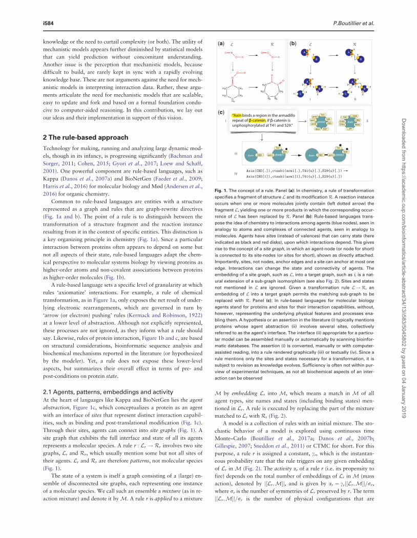
Fig. 1. The concept of a rule. Panel (a): In chemistry, a rule of transformation
specifies a fragment of structure L and its modificationR. A reaction instance
occurs when one or more molecules jointly contain (left dotted arrow) the
fragment L, yielding one or more products in which the corresponding occur-
rence of L has been replaced by R. Panel (b): Rule-based languages trans-
pose the idea of chemistry to interactions among agents (blue nodes), seen in
analogy to atoms and complexes of connected agents, seen in analogy to
molecules. Agents have sites (instead of valences) that can carry state (here
indicated as black and red disks), upon which interactions depend. This gives
rise to the concept of a site graph, in which an agent-node (or node for short)
is connected to its site-nodes (or sites for short), shown as directly attached.
Importantly, sites, not nodes, anchor edges and a site can anchor at most one
edge. Interactions can change the state and connectivity of agents. The
embedding of a site graph, such as L, into a target graph, such as i, is a nat-
ural extension of a sub-graph isomorphism (see also Fig. 2). Sites and states
not mentioned in L are ignored. Given a transformation rule L ! R, an
embedding of L into a target graph permits the matching sub-graph to be
replaced with R. Panel (c): In rule-based languages for molecular biology
agents stand for proteins and sites for their interaction capabilities, without,
however, representing the underlying physical features and processes ena-
bling them. A hypothesis or an assertion in the literature (i) typically mentions
proteins whose agent abstraction (ii) involves several sites, collectively
referred to as the agent’s interface. The interface (ii) appropriate for a particu-
lar model can be assembled manually or automatically by scanning bioinfor-
matic databases. The assertion (i) is converted, manually or with computer-
assisted reading, into a rule rendered graphically (iii) or textually (iv). Since a
rule mentions only the sites and states necessary for a transformation, it is
subject to revision as knowledge evolves. Sufficiency is often not within pur-
view of experimental techniques, as not all biochemical aspects of an inter-
action can be observed
i584 P.Boutillier et al.
Dow
nloaded from https://academ
ic.oup.com/bioinform
atics/article-abstract/34/13/i583/5045802 by guest on 04 January 2019

distinguishable with respect to the mechanism expressed in r. The
activity ar is the stochastic rule-based analog of the flux through a
reaction in standard chemical kinetics. If a reaction event occurs at
time t, then the probability that r is applied to one of its embeddings
is given by its relative activity ar=P
s as.
Even when the set of all reachable molecular species and their
reactions can be deduced from a given collection of rules, the size of
the resulting network is often too large to be handled explicitly.
Importantly, translating rules into kinetic differential equations based
on an explicit reaction network would miss the point of rule-based
approaches entirely. Rules provide compactness, transparency and a
handle on combinatorial complexity; and, perhaps most significantly,
systems of rules constitute a more appropriate level for causal analysis
than reaction networks, because reasoning at the level of rules avoids
contamination with context that defines a reaction but is irrelevant to
the application of the underlying rule (Figs 1b and 2).
2.2 SyntaxFrom here on our discussion refers specifically to the Kappa frame-
work (https://kappalanguage.org). Graphs are the proper formal
objects in this framework, but we need a textual notation for con-
venience. The binding state of a site s is specified in square brackets:
s[.] indicates that s is free (unbound), whereas s[n] (n a non-
negative integer) is bound to the unique other site in the same ex-
pression whose binding state is also n. Thus, A(x[2]), B(y[2]) asserts
that agent A is bound at x to agent B at y. Given an agent type with
two binding sites, A(x, y), a simple rule might be, bnd: A(x[.]),
A(y[.])! A(x[1]), A(y[1]). This rule yields ‘head-to-tail’ polymeriza-
tion, because it is matched by any two asymmetric ends (sites x and
y). Rule bnd, therefore, generates linear polymers and rings of any
size, limited only by the available pool of agents of type A. A site z
can also have an internal state, expressed as a string between curly
braces. The internal state is typically used to specify a post-
translational modification. Thus, C(z{p}[.]) denotes an agent of type
C whose site z is in state p (phosphorylated, say) and unbound.
When writing patterns, such as observables or rules, states not
mentioned do not constrain their matchings into the mixture (‘don’t
care, don’t write’). For example, C(z{p}) is matched by any instance
of C phosphorylated at z regardless of its binding state. An extensive
manual (Boutillier et al., 2017b) provides many details beyond the
present scope.
3 Materials and methods
3.1 Kappa software agentsThe main Kappa ecology consists of several software agents that com-
municate through an ad hoc JSON-based protocol and expose high-
level functionalities through both a Python API and an HTTP REST
service. At present these are: The Kappa Simulator (KaSim), the Kappa
Static Analyzer (KaSA) and the Kappa Story Extractor (KaSTOR). A
Python client enables scripting to tailor work flows and is available as
the kappy package in pip. Modeling in a rule-based language is much
like writing large and complex programs, which necessitates an inte-
grated development environment. To integrate the new Kappa web
services, we developed a browser-based User Interface (UI), which also
comes packaged as a self-contained application for the Windows OS,
Mac OS and Ubuntu. This effort raised several challenges pertaining to
visualization and analysis that we address below.
The KaSim is an implementation of CTMC designed for rule-
based models with particular emphasis on scalability in typical usage
regimes (Danos et al., 2007b). A recent optimization targets a costly
step in the CTMC core loop (Boutillier et al., 2017a). After a rule
has been applied to the mixture, rule activities (Section 2.1) must be
updated by identifying all embeddings that were gained or lost
(Fig. 2) and likewise for updating counts of user-defined observ-
ables. The optimization consists in the initial construction of a
model-dependent data structure by virtue of which no pattern—
whether the left side of a rule, a user-defined observable, or any sub-
pattern of these—is ever scanned twice for the same embedding into
the mixture. For example, if two left sides Lr and Ls have a common
sub-pattern, any match to that sub-pattern is shared during the at-
tempt at extending the match to Lr and Ls.
KaSim is interactive, allowing a simulation to be paused and
resumed at any time. A versatile intervention language can be used
for defining perturbations, such as altering rate constants and add-
ing/removing agents interactively or at time points set in the input
file. The intervention language supports queries about the state of
the system and requests for data dumps, such as snapshots of the
mixture and rule influence matrices (Section 3.3).
Simulation is the main tool for studying the dynamical behavior
of a rule-based model. However, some properties of a model can be
determined by direct inspection and manipulation of the rules with-
out execution. Such properties are static in the sense of being time-
independent, yet they relate to behavior because they demarcate its
envelope. For example, a static property is the reachability of a spe-
cific molecular species, i.e. an answer to the question whether a
given species (or pattern) can in principle be produced by the joint
operation of the rules. Another static property is the impossibility of
a rule to ever fire because its L-pattern can never be matched
(Section 3.2). Further properties are the existence of invariants, such
as between states at two sites of the same agent (i.e. assertions of the
kind ‘whenever site s is phosphorylated, site p is bound to agent D’).
The firing of a rule r could create a configuration that partially satis-
fies the Ls of another rule s, thus potentially contributing to an in-
crease in the activity of s. Similarly, r might compete with s for
instances, thus potentially decreasing the activity of s. Such potential
influence (positive, negative, or none) is also a static property.
Fig. 2. Rule application. Rule r asserts a simple mechanism in which the dis-
sociation of agents of type A from those of B at their respective sites s (the
name of a site has no formal meaning and is local to an agent) is independent
of the state at all other sites. The bottom left depicts a simple mixture M of
two molecular species, i and ii, each present in a single instance. Agents of
type A and B have more sites than are mentioned in the rule; black and red
dots indicate a post-translational modification (phosphorylation status, say).
L has three possible embeddings in M. An embedding is a sub-graph iso-
morphism respecting the type of agents and the state (including connectivity)
of sites mentioned. The propensity of r to fire in M is therefore 3cr , as each
embedding is equally likely to be chosen. Species ii allows for two possible
embeddings and will react twice as fast than species i. After application of r,
the mixture has changed and a new molecular species iii has appeared
The Kappa platform for rule-based modeling i585
Dow
nloaded from https://academ
ic.oup.com/bioinform
atics/article-abstract/34/13/i583/5045802 by guest on 04 January 2019

In Section 3.3, we look at the actual influence that rules have on
each other, which is a dynamic property. Static properties are espe-
cially helpful in debugging a model, as they can quickly pinpoint
discrepancies between expected and actual behavior. The KaSA
supports all these analyses. It relies heavily on a technique called
‘abstract interpretation’, described in Section 3.2.
A third tool is the KaSTOR which aims at providing insights into
how an event of interest (EOI) occurred in a particular event trace
obtained by simulation of a model. The underlying concepts offer a
distinctive perspective on (mechanistic) causality in molecular sys-
tems. We outline their implementation in Section 3.4.
3.2 Static analysis and abstract interpretationThe formal analysis of graph-rewrite systems relies heavily on eluci-
dating the relationships between graph-morphisms, for which cat-
egory theory provides a powerful framework. Yet, in practice,
computing an exact answer to problems like enumerating the set of
reachable species is not feasible, because of numbers beyond imagin-
ation. Static analysis algorithms written for Kappa achieve practical
utility by deploying an approach known as abstract interpretation
(Cousot and Cousot, 1977), wherein the given rules are made more
abstract in the sense of systematically discarding specific informa-
tion. The reachability problem is then approached within the set of
abstract rules, where it can be handled faster at the price of an over-
approximated rather than exact solution.
Central to the abstract interpretation technique in Kappa is the
concept of a local view. The local view of an agent A that occurs in
a site graph G consists of A itself, its sites and their state as men-
tioned in G, alongside information about which sites of A are bound
to which site of which agent type, i.e. without including the bound
agent and any additional information about it. For example, in
Figure 3, the local view of the first agent (labelled ‘1’) of type A is
given by ii, which consists of A, site d bound to site d of another
agent of type A (but without including that agent, hence the dotted
outline) and site s bound to site s of an agent of type B. We can think
of such linkage information as a bond ‘stub’, expressed syntactically
as A(s[s.B], d[d.A]). The local view of the other A-agent (labelled
‘2’) is the same. Thus, the complex i yield a set of three distinct local
views {ii, iii, iv}. This step is called abstraction, denoted by k �ð Þ.Continuing the example, we can stitch the local views back together
using the information in the bond ‘stubs’. Doing this in all possible
ways yields the set of four complexes shown in Figure 3. This step is
called concretization. Clearly, the abstraction step for agent A loses
information about the phosphorylation state of the B bound to it.
The concretization step reconstructs the original complex, but also
others—an overapproximation. We apply this idea to the left sides
Lr and right sides Rr of each rule r in a model. In this way, Lr !Rr
is replaced by an abstract version k Lrð Þ ! k Rrð Þ cast entirely in
terms of local views. It turns out that the fixed point obtained from
the forward closure of abstract rules always exists and is finite (even
for systems capable of generating infinitely many species). It can be
further shown that stitching together these local views in all admis-
sible ways yields a superset of the true reachable molecular species
(Danos et al., 2008). Because of overapproximation, a species Q in
the superset obtained from abstraction may not be reachable with
the original rules. However, if Q is not in the superset, it cannot be
reached by the original rules either: A no is a no, and a yes is a
maybe. The most recent version of KaSA generalizes local views to
more flexibly compromise between accuracy, efficiency and expres-
sivity (Feret and L�y, 2018).
This technique makes reachability analysis fast enough to permit
computing, thus visualizing, contact maps (CMs; Section 4.1) and
rule influence maps in real-time as a user updates a model. This in
turn makes abstract reachability useful in debugging a model, which
is a process that furthers understanding.
As a simple example of KaSA’s operation consider the following
minimal model snippet. (Rate constants are ignored by static analysis;
they only serve the purpose of getting the model past the parser).
%init: 1 E ()
%init: 1R ()
’r1’ E(x[.]), R(x[.]) -> E(x[1]), R(x[1]) @0
’r2’ E(x[1]), R(x[1], c[.]) ->
E(x[.]), R(x[.], c[.]) @0
’r3’ R(x[_], c[.]), R(x[_], c[.]) ->
R(x[_], c[1]), R(x[_], c[1]) @0
’r4’ R(c[1], cr[.], n[.]), R(c[1], cr[.], n[.]) ->
R(c[.], cr[.], n[.]), R(c[.], cr[.], n[.]) @0
’r5’ R(c[1], cr[.], n[.]), R(c[1], cr[.], n[.]) ->
R(c[1], cr[2], n[.]), R(c[1], cr[.], n[2]) @0
’r6’ R(cr[1]), R(n[1]) -> R(cr[.]), R(n[.]) @0
’q1’ R(x[.], c[.], cr[_], n[_]) ->
R(x[.], c[.], cr[_], n[_]) @0
’q2’ R(c[1], cr[2]), R(c[1]), R(n[2]) ->
R(c[1], cr[2]), R(c[1]), R(n[2]) @0
This snippet is a simplified version of reversible receptor/ligand
binding (‘r1’,‘r2’), receptor dimerization (‘r3’,‘r4’) and internal
crosslinking (‘r5’,‘r6’). (The underscore denotes a bound state with-
out caring about the type of binding partner.) To query the static
analyzer about the reachability of patterns of interest, we defined
two identity rules, ‘q1’ and ‘q2’ (in which Lqf1;2g ¼ Rqf1;2g), to ex-
ploit KaSA’s detection of dead rules. Dead rules are rules that can-
not fire because their left side pattern is unreachable. As soon as ‘q1’
and (or) ‘q2’ are added to ‘r1’–‘r6’ in the UI editor, KaSA flags them
as unreachable. For ‘q1’ this means that a receptor cannot be cross-
linked unless it is bound to ligand (but no single rule explicitly states
that); for ‘q2’ this means that the bonds at sites c and cr of a receptor
must both engage the same second receptor, i.e. no receptor triples.
KaSA came to this conclusion by automatic abstract interpretation.
The analysis made use of the initialization statements (‘init’) for lig-
and E and receptor R. (Static analysis only cares whether the initial
copy number is non-zero.) If we remove the first statement, KaSA
responds in real-time by flagging all rules as unreachable—because
of the absence of ligand. This can be useful to ensure that the initial
condition of complex models covers the intended agent types. The
command line version of KaSA provides many additional analyses
that are not yet exposed in the software agent.
3.3 The dynamic influence networkThe dynamic influence network (DIN) is a construct for tracking the
way rules influence each other over time. Its visualization is dis-
cussed in Section 4.3.
Fig. 3. Abstract interpretation. Complex (i) is ‘exploded’ into its local views
(ii), (iii) and (iv) by an abstraction process k described in the main text. The
concretization process c stitches the local views back into complexes, repro-
ducing the original, but also others, reflecting the fact that information was
abstracted away. Reachability via local views is a fast overapproximation,
enabling useful real-time analysis that would otherwise be prohibitive
i586 P.Boutillier et al.
Dow
nloaded from https://academ
ic.oup.com/bioinform
atics/article-abstract/34/13/i583/5045802 by guest on 04 January 2019

A rule r fires with a probability proportional to its activity ar
(Section 2.1). When r fires, it alters the state of the mixture M,
which can affect the activity of rule s by generating or destroying
matchings to Ls inM. Fix a time interval t; t þ s½ � and let i index the
events that occur in that interval. The ith event causes a transition
from stateMi (before the event) toMiþ1 (after the event). If the ith
event is due to the firing of r, its contribution to the relative change
in the activity of s, denoted by DIr;s ið Þ, is given by
DIr;s ið Þ ¼as iþ 1ð Þ � as ið Þ
as ið Þ if i is due to r and as ið Þ 6¼ 0
0 otherwise
8><>:
(1)
We aggregate these contributions during the interval t; t þ s½ � and
divide by the number nr of r-events to obtain the average influence
of r on s during that interval:
DIr;s t; sð Þ ¼ 1
nr
Xi in
t;tþs½ �
DIr;s ið Þ; (2)
with the events i occurring in t; t þ s½ �. We refer to the matrix
Equation (2) as the DIN. The nodes of the DIN are rules and an
edge between r and s has weight DIr;s t; sð Þ.
3.4 Causal lineages and compressionKaSim can output the whole sequence of events generated by a simu-
lation. This is called a trace. The traces of models we work with
comprise routinely many millions of events. A persistent challenge is
to extract an explanation of how an EOI specified by the user actu-
ally occurred in a particular run.
Given a trace s, i.e. a sequence of events s ¼ e1e2 � � � en to an EOI
(EOI � en), we first identify which events were on the path to the EOI
and in which causal order, as the temporal sequence of events may not
always be relevant in stochastic systems with concurrency. Two tem-
porally adjacent events e1e2 are concurrent if they can occur in any
order—e1e2 or e2e1—while having the same effect, otherwise there is a
relation of precedence between them. For e1 to precede e2 means that
the rule underlying e1 contributes to satisfying a condition required by
the left-hand side of the rule underlying e2. The naive approach we take
here is to view causality as the opposite of concurrency, i.e. a relation
of precedence. Not all precedence is causal, however. Suppose a kinase
can phosphorylate a substrate and, independently, the substrate can be
degraded. Whenever phosphorylation is observed, it must precede deg-
radation, but, given our assumption, we cannot say that phosphoryl-
ation caused degradation.
We now wish to identify the events in s that were involved in
bringing about the EOI while revealing their precedence relations.
Figure 4 illustrates the method by means of a simple example.
Assume the EOI is the production of a free phosphorylated substrate
in the following Michaelis–Menten type of model:
’b’ K(z[.]), S(x[.], y{u}) ->
K(z[1]), S(x[1], y{u})
’u’ K(z[1]), S(x[1]) -> K(z[.]), S(x[.])
’p’ K(z[1]), S(x[1], y{u}) ->
K(z[1]), S(x[1], y{p})
’*’ S(x[.], y{p}) -> S(x[.], y{p})
Since causality is a relation between events, the identity rule ‘*’
serves to transform our query into an event. Suppose a particular
mixture contains three substrate agents S and two kinase agents
K and that a simulation happened to produce the trace
s ¼ bbubpuppu�, where each event is labeled by the rule that
produced it and contains information about which agent identifiers
matched the rule. KaSTOR, the causal analysis software agent,
attaches to every site of every agent instance in the mixture a thread
and records whether an event only tested the state of a site or
whether it also modified it. In typical Kappa rules, a modification
also implies a test. This results in the representation depicted in
Figure 4a, where threads run vertically and events horizontally with
markings—black filled circles if the thread was modified, white if it
was only tested. To reconstruct the causal past of ’*’, we slide its
tests backward in time following the instructions shown in
Figure 4b. Consider an event e followed by event e0 and ask for every
site involved in e0 whether the test or modification of that site could
have occurred before e. If this is the case, slide that test or modifica-
tion backwards in time past e and repeat that question against the
event that occurred prior to e, etc. A test of the state at a particular
site in event e0 can always slide past a test (or absence thereof) for
the same site in event e, as it will not invalidate the occurrence of e.
A test associated with event e0 cannot slide past a modification asso-
ciated with event e, or e0 could not have occurred. This generates a
causal arrow from e to e0. A modification cannot slide past a modifi-
cation for the same reason. Lastly, a modification can slide past a
test, but this is a case of non-causal precedence discussed above and
is annotated by adding a ‘prevention arrow’ from e0 to e.
This procedure, applied to our trace, will discard any events that
had no bearing on the EOI (Fig. 4d), while producing a directed
acyclic graph representing the precedence structure of its causal past
(Fig. 4c). Figure 4c reads: S2 binds K1, then they dissociate, then K1
binds S1, then they dissociate; then K1 rebinds S2, then K1 phosphor-
ylates S2 and precedes (non-causally) the dissociation of K1 from S2,
thus causing the EOI. The problem is that events in the causal past
of an EOI often violate necessity. In our example, the detour
(a)
(b) (d)
(c) (e)
Fig. 4. Causal analysis of event traces. Panel (a): The representation of a trace
in terms of ‘worldlines’ that record the modifications and tests at each site for
each event in the trace. Panel (b): Schematic of allowed moves and annota-
tions emitted when swapping the order of adjacent events for a particular
wordline (i.e. site in the model). See text for details. Panel (c): The causal past
of the EOI reconstructed from the trace representation in panel (a) following
the instructions in panel (b). Panel (d): The events that had no bearing on the
EOI. Panel (e): Minimization of the causal past shown in panel (c) by eliminat-
ing cycles that return to an equivalent system state from the point of view of
the EOI
The Kappa platform for rule-based modeling i587
Dow
nloaded from https://academ
ic.oup.com/bioinform
atics/article-abstract/34/13/i583/5045802 by guest on 04 January 2019
through S1, although it occurred, was not necessary, since event e7
could have happened instead of e1 yielding the same result. One way
to isolate necessity is to search, within the causal past reconstructed
by the previous procedure, for a minimal sub-set of events that can
produce the EOI (Danos et al., 2012). We call this minimization
causal compression. KaSTOR automatically translates a causal past
into a propositional formula in which each event is associated with
a Boolean variable whose value determines whether the event is kept
or discarded. Each scenario has implications for which other events
must be retained or discarded to ensure that the EOI obtains.
KaSTOR then seeks the smallest number of propositional variables
that, when set to true (keep), satisfy the formula. This is done with
KaSTOR’s own SAT solver tailored to the structure of this problem.
The result is the compressed causal past of Figure 4e, which we call
a story. A more realistic case of causal compression is touched upon
in Section 4.4 and Figure 8.
4 Results
The Kappa UI is a suite of interactive visualization tools, integrating
various services in the Kappa ecology. Here, we provide details
about the Kappa CM, the snapshots tool, the DIN visualization
(DIN-Viz) and our initial efforts in visualizing stories created with
KaSTOR.
A range of projects introduce techniques for visualizing protein–
protein interaction networks in support of analysis (Murray et al.,
2017). Kohn et al. (2006) introduce a technique that visualizes regu-
latory networks, but is not rule-based in the sense defined here.
Chylek et al. (2011) provide guidelines for visualizing and annotat-
ing rule-based models extending the notion of CM (Danos et al.,
2007a). Smith et al. (2012) develop the RuleBender framework for
editing and exploring rule-based systems. This is taken further by
Sekar et al. (2017), in particular by grouping and merging rules into
a more compact diagrammatic representation. Dang et al. (2015)
present a visualization technique that uses animation to highlight
causal relationships within pathways, and Paduano and Forbes
(2015) explore interactive methods to visualize common patterns in
biological networks.
4.1 Visualization: the CMThe CM of a model is a generalized site graph in which every agent
type occurs exactly once and every site exhibits all bonds and states
that are possible according to the rules. The CM is generated auto-
matically. For smaller to moderately sized models, its construction
and visualization are updated in real-time while a user is writing
rules in the UI text editor. The CM allows a user to quickly check
visually whether a molecular species is admissible in principle. The
static analyzer KaSA can constrain the CM based on abstract reach-
ability, as outlined in Section 3.2. The most immediate utility of
such visualization is in debugging. For example, a missing arc,
where a modeler expected to see one, might indicate an omitted,
mistyped, or unreachable rule.
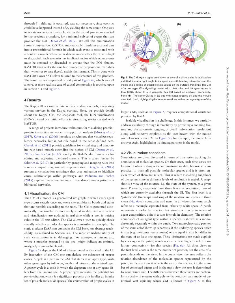
Figure 5a depicts the CM of a large model as rendered in the UI.
By inspection of the CM one can deduce the existence of proper
cycles. A cycle is a path in the CM that starts at an agent type, visits
other agent types by following bonds and returns to the original type.
A proper cycle is a cycle in which the departure site at any agent dif-
fers from the landing site. A proper cycle indicates the potential for
polymerization, which is a significant property as it implies an infinite
set of possible molecular species. The enumeration of proper cycles in
larger CMs, such as in Figure 5, requires computational assistance
provided by KaSA.
Scalable visualization is a challenge. In this instance, we partially
address scalability through interactivity by providing a zooming fea-
ture and the automatic toggling of detail (information resolution)
along with selective emphasis as the user hovers with the mouse
over elements of the CM. In Figure 5b, for example, the mouse hov-
ers over Axin, highlighting its binding partners in the model.
4.2 Visualization: snapshotsSimulations are often discussed in terms of time series tracking the
abundance of molecular species. On their own, such time series are
less useful when dealing with combinatorial models, because it is im-
practical to track all possible molecular species and it is often un-
clear which of them are salient. This is where visualizing snapshots
of the system state at different levels of resolution is useful. A snap-
shot is a view of the mixture, i.e. the state of the system, at a given
time. Presently, snapshots have three levels of resolution, two of
which are currently available through the UI. The first level is a
‘patchwork’ (treemap) rendering of the mixture and comes in three
views (Fig. 6a–c): count, size and mass. In all views, the term patch
refers to a rectangle separated from others by white space. A patch
represents a molecular species, but visualizes it only in terms of
agent composition, akin to a sum formula in chemistry. The relative
abundance of an agent type within a species is shown as a mono-
chromatic rectangle within the patch. Two monochromatic patches
of the same color show up separately if the underlying species differ
in size (e.g. monomer versus n-mer) or are equal in size but differ in
the state of at least one agent. These distinctions are made explicit
by clicking on the patch, which opens the next higher level of reso-
lution—connectivity—for that species (Fig. 6d). All three views at
the first level contain the same number of patches, but the area of a
patch depends on the view. In the count view, the area reflects the
relative abundance of the molecular species represented by the
patch; in the size view it reflects the size of the species, i.e. the num-
ber of connected agents and in the mass view the area is determined
by count times size. The differences between these views are particu-
larly notable in systems with polymerization, such as a model of ca-
nonical Wnt signaling whose CM is shown in Figure 5. In this
(a) (b)
Fig. 5. The CM. Agent types are shown as arcs of a circle; a site is depicted as
a dotted line at a right angle to its agent arc with binding interactions on the
inside and a listing of possible state values on the outside. Panel (a): The CM
of a prototype Wnt signaling model with 1440 rules and 19 agent types. It
took KaSA about 18 s to generate this CM based on abstract reachability.
Panel (b): The same CM as in (a) but with states toggled off and the mouse
over Axin (red), highlighting its interconnections with other agent types of the
model
i588 P.Boutillier et al.
Dow
nloaded from https://academ
ic.oup.com/bioinform
atics/article-abstract/34/13/i583/5045802 by guest on 04 January 2019

system, several scaffold proteins can form a polymeric structure, ei-
ther alone or in interaction with each other (Fiedler et al., 2011).
We illustrate the patchwork view by comparing the state of the
system before (–) to that after (þ) Wnt addition. In both cases the
most frequent components in the count view are homogenous, main-
ly protomers or dimers of scaffolds like Dvl, APC and LRP6. The
size view, however, is dominated by a large composite polymer—so
large that it also dominates the mass view. Prior to Wnt addition,
the polymer has the composition of a so-called ‘destruction com-
plex’, which targets b-catenin (CTNNB1) for degradation. The be-
fore/after comparison in the size view yields the following
observations. (i) The largest complex has increased in size. (ii) The
largest complex has changed composition, gaining a large mass of
Dvl (dark brown), previously spread across a variety of separate
entities. (iii) The rest of the mixture has become far more frag-
mented by a greater diversity of smaller species. (iv) The diversity of
LRP6 (dark pink) states has increased—prior to Wnt we recognize a
few patches in the lower right corner of the size view, while there
are many more monochromatic LRP6 patches after Wnt addition.
This is more conspicuous in the count view. (v) Proteins that were
associated with Dvl prior to Wnt addition (especially Fzd) have now
been pulled into the giant component, representing the migration of
the destruction complex machinery to the membrane where it inter-
acts with trans-membrane proteins, such as Fzd and CK1d. (vi) The
giant component from the pre-Wnt state has lost a large amount of
APC, which is now found in isolated association with b-catenin.
(vii) Complexes with a composition of more than four agent types
are more frequent. Prior to Wnt addition, the only complex with
more than four agent types was the destruction aggregate, whereas
afterwards the giant component increased in compositional diversity
and so did species not connected to it.
Such observations are drawn more readily from patchwork dia-
grams than time series, especially if it is unclear what to look for at
the outset. Patchwork diagrams lay out an overall view of a suitably
coarse-grained system state and seem especially conducive for quali-
tative comparisons. The observations made here, regardless of their
biological significance, also illustrate the complexity of phenomena
that can arise with a mere dozen agent types—a complexity that
would be difficult to capture without a rule-based platform with an
integrated visualization environment.
A higher level of informational resolution is accessed when click-
ing on patches to reveal the connectivity structure of the underlying
molecular species, as shown for the pre-Wnt case in Figure 6d. The
polymeric cross-linked structure dominating the pre-Wnt regime is
shown on the left of that panel, alongside with the second largest
structure, revealing a completely segregated aggregate of Dvl. At
this resolution, the structures do not exhibit (internal) state and site
information, which would not be cognitively scalable. The next level
of resolution consists in revealing detailed (local) state information
in a split view for any agent that the user hovers over in the connect-
ivity view. An interactively accessible resolution hierarchy increases
the effectiveness of the patchwork view.
4.3 Visualization: the DINKaSim can be directed to compute influence matrices DIr;s t; sð Þ,Equation (2), aggregated over user-specified time intervals t; t þ s½ �.Typically, s and increments in t are chosen so as to create overlap-
ping intervals for smoothness. A time series of such matrices can be
uploaded to the DIN visualization server (DIN-Viz) (https://github.
com/CreativeCodingLab/DynamicInfluenceNetworks), where the
DIN is presented as a node-link diagram, leveraging a force-directed
layout to position related nodes and clusters near to each other. The
nodes represent the rules and the links convey the influence of rules
on each other, color-coded with red (green) signifying a negative
(positive) influence. This visualization enables the topological ana-
lysis of rule-fluxes in a KaSim simulation at the chosen time step
scale. By mapping the magnitude of influence to the link strength,
highly mutually influential rules are closely grouped together visual-
ly. This provides insight as to which rules might (temporarily) con-
spire in producing a pathway.
In order to further facilitate the analysis of these highly related
rules, we perform a clustering operation on the network based on
the influence between rules to generate groups with a high inner in-
fluence, based on a user-selected threshold. The absolute value of in-
fluence between rules, determines the attractive link forces in the
network. DIN-Viz maps the number of firings of a rule (during
(a) (b)
(c) (d)
Fig. 6. Snapshots. Panels (a), (b), (c): The patchwork diagrams depict three views of the system state at the resolution of agent composition. See text for details.
The diagrams refer to the Wnt model with CM shown in Figure 5. For each view the snapshot was taken at steady state prior and after Wnt addition. Panel (d):
The next higher level of snapshot resolution exhibits agent connectivity for a patch clicked by the user. The connectivities shown pertain to the two complexes
indicated in the size view
The Kappa platform for rule-based modeling i589
Dow
nloaded from https://academ
ic.oup.com/bioinform
atics/article-abstract/34/13/i583/5045802 by guest on 04 January 2019

t; t þ s½ �) to the node size, and the influence of one rule on another
to the link width. We indicate the directionality of a link and the
sign of the influence by using directional color gradients. Figure 7
uses yellow-to-red for negative and yellow-to-green for positive;
colorblind-safe colormaps are also available.
Details-on-demand are available for each link, showing the
source and target, as well as the exact influence value; similarly,
hovering over a rule (node) shows the rule name, the amount of self-
influence and the rule’s top incoming and outgoing influences. The
user may also choose to make visible the names of the rules as labels,
either for all rules, or for interactively selected rules.
To represent the dynamism of the system, animation is used to
update the influence between the rules, which in turn updates the
edge weights, node sizes and cluster definitions. A time slider con-
trols the current time step, enabling the user to move through time
or jump to a particular time step. Standard playback controls ani-
mate the simulation so that the user can observe changes in the DIN
over time.
Although force-directed layouts mitigate visual clutter in node-
link diagrams, dense networks can still be difficult to make sense
of—an issue that is exacerbated when representing large datasets.
DIN-Viz enables the user to manually create a layout of nodes or en-
tire clusters through relocating and ‘pinning’ them to specified loca-
tions. This reorganization reduces clutter, but also helps users to
distribute rules and clusters in a way that is cohesive with their
thought process during exploratory analysis. When pinned, the spa-
tial positioning and grouping of selected rules and clusters is pre-
served over the course of the entire animation, over-riding the
normal layout behavior.
While the mathematically defined clusters capture groups of
rules that influence one another, there may be rules which are
related through their behavior but lack a strong influence with one
another. To solve this problem, we implement a ‘painting’ inter-
action. The user can provide a color marking to nodes to indicate
that they are grouped together, and then insert them into an existing
or newly created cluster. These categorical groupings, similar to the
spatial groupings achieved through pinning, aid in the logical organ-
ization of rules during analysis by the user.
As a use case we analyze a rule-based model of the autonomous
KaiABC circadian oscillator in the cyanobacterium Synechococcus
elongatus. We forgo a detailed description of the molecular biology
and of the Kappa model, which closely follows the literature
(van Zon et al., 2007), in favor of a broader outline illustrating the
reasoning enabled by the DIN and its visualization.
The KaiABC system consists of three proteins, A, B and C. C can
be phosphorylated and dephosphorylated at multiple sites, thereby
assuming distinct phosphorylation levels (p-levels for brevity). It
also can switch between two conformational states, A and I. At low
p-levels C prefers the A-state. The probability of a flip from A to I
increases with increasing p-level. When C is in the A-state, it binds A
with an affinity that decreases rapidly with increasing p-level. Upon
binding A, C gets locked into the A-state, which promotes phos-
phorylation. As the p-level increases, A dissociates from C, allowing
it to flip into the I-state, which favors dephosphorylation. This pro-
cess results in a p-level oscillation of individual C molecules. Since
these oscillations are not coordinated, no p-level oscillations will
occur at the macroscopic level of the C-population. Co-ordination
between C proteins is achieved by B, which binds C in the I-form.
Once bound, B locks C into the I-form, facilitating dephosphoryla-
tion. Crucially, once bound to C, B also binds A with an affinity
that is maximal at intermediate p-levels of C. By sequestering A in a
mechanism that depends on C molecules that are late in the cycle, B
holds back the phosphorylation of C molecules that are ahead in the
cycle, statistically synchronizing the individual cycles and resulting
pC_1 pC_1_op
pC_2 pC_2_op
pC_3 pC_3_oppC_4 pC_4_oppC_5 pC_5_op
pC_6 pC_6_op
flip_0 flip_0_opflip_1 flip_1_opflip_2 flip_2_opflip_3
A.Ca
B.Ci1_0
B.Ci1_0_op
B.Ci2_0
B.Ci2_0_op
B.Ci1_g0
B.Ci1_g0_op
B.Ci2_g0
B.Ci2_g0_op
A..BA.B1_1
A.B1_2A.B1_3
A.B1_4
A.B2_1
A.B2_2
A.B2_3
A.B2_4
flip_4 flip_4_opflip_5 flip_5_opflip_6 flip_6_op
A..Ca_0A..Ca_1
A..pC_2
A..Ca_3
A..Ca_4
A..Ca_5
A..Ca_6A..pC_1
A..Ca_2
A..pC_3A..pC_4A..pC_5A..pC_6
t=58 t=67
0 30 60 90 120
Time: 57.9-58.2
1e-8 1e-6 1e-4 1e-2
Influence > 7.97e-8Clustering Visibility
0 30 60 90 120
Time: 66.9-67.2
1e+0 1e+5 1e+10
Influence > 0.0399Clustering Visibility
50 54 58 62 66 70 74 78 82 86 900
0.2
0.4
0.6
0.8
50 54 58 62 66 70 74 78 82 86 900
0.2
0.4
0.6
0.8
Time [h]
Aver
age
phos
phor
ylat
ion
leve
l
(a) (b) (c) (d)
i ii
iii
viiviii
iiiiii
iv
v vi
Fig. 7. DIN and DIN-Viz. Panel (a): System level activity of the KaiABC oscillator. The ordinate is the overall fractional phosphorylation in the system, defined asPni¼1 i ½CðiÞ�=ðn
Pni¼1½CðiÞ�Þ, where ½CðiÞ� is the abundance of KaiC proteins whose p-level is i; here n¼ 6. Panels (b) and (c): DIN snapshots at the cycle phases indi-
cated by the dots in panel (a). Panel (d): An interactive feature of the DIN-Viz highlights the targets of the influences originating from a rule when the user selects it
Fig. 8. Causal compression in early EGF signaling. The concepts of Figure 4
are illustrated in the case of Sos recruitment
i590 P.Boutillier et al.
Dow
nloaded from https://academ
ic.oup.com/bioinform
atics/article-abstract/34/13/i583/5045802 by guest on 04 January 2019
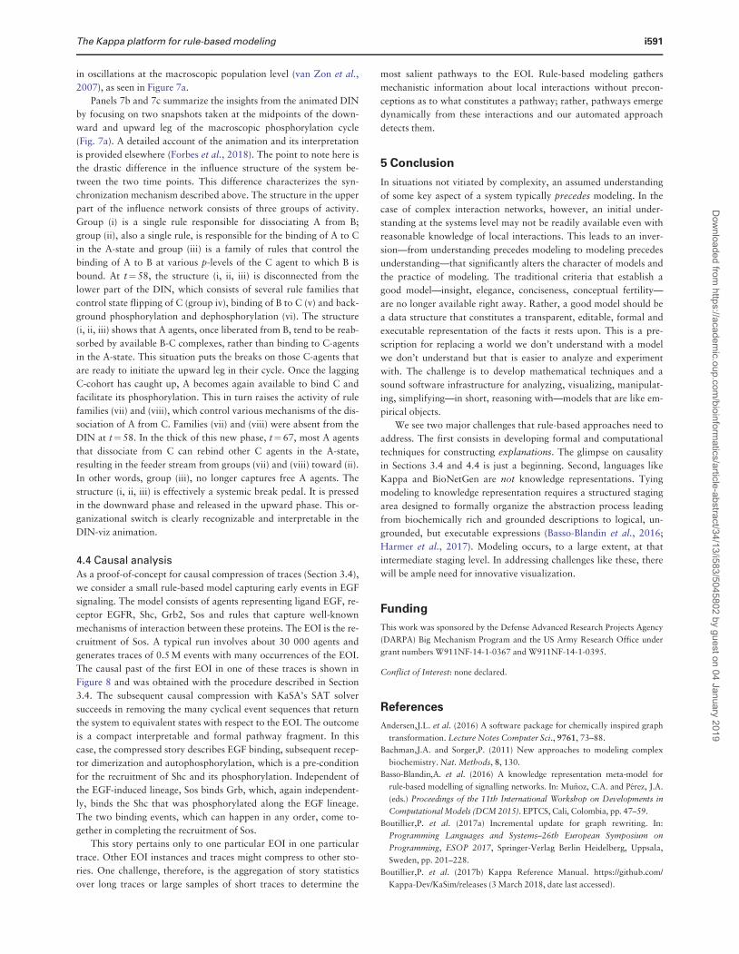
in oscillations at the macroscopic population level (van Zon et al.,
2007), as seen in Figure 7a.
Panels 7b and 7c summarize the insights from the animated DIN
by focusing on two snapshots taken at the midpoints of the down-
ward and upward leg of the macroscopic phosphorylation cycle
(Fig. 7a). A detailed account of the animation and its interpretation
is provided elsewhere (Forbes et al., 2018). The point to note here is
the drastic difference in the influence structure of the system be-
tween the two time points. This difference characterizes the syn-
chronization mechanism described above. The structure in the upper
part of the influence network consists of three groups of activity.
Group (i) is a single rule responsible for dissociating A from B;
group (ii), also a single rule, is responsible for the binding of A to C
in the A-state and group (iii) is a family of rules that control the
binding of A to B at various p-levels of the C agent to which B is
bound. At t¼58, the structure (i, ii, iii) is disconnected from the
lower part of the DIN, which consists of several rule families that
control state flipping of C (group iv), binding of B to C (v) and back-
ground phosphorylation and dephosphorylation (vi). The structure
(i, ii, iii) shows that A agents, once liberated from B, tend to be reab-
sorbed by available B-C complexes, rather than binding to C-agents
in the A-state. This situation puts the breaks on those C-agents that
are ready to initiate the upward leg in their cycle. Once the lagging
C-cohort has caught up, A becomes again available to bind C and
facilitate its phosphorylation. This in turn raises the activity of rule
families (vii) and (viii), which control various mechanisms of the dis-
sociation of A from C. Families (vii) and (viii) were absent from the
DIN at t¼58. In the thick of this new phase, t¼67, most A agents
that dissociate from C can rebind other C agents in the A-state,
resulting in the feeder stream from groups (vii) and (viii) toward (ii).
In other words, group (iii), no longer captures free A agents. The
structure (i, ii, iii) is effectively a systemic break pedal. It is pressed
in the downward phase and released in the upward phase. This or-
ganizational switch is clearly recognizable and interpretable in the
DIN-viz animation.
4.4 Causal analysisAs a proof-of-concept for causal compression of traces (Section 3.4),
we consider a small rule-based model capturing early events in EGF
signaling. The model consists of agents representing ligand EGF, re-
ceptor EGFR, Shc, Grb2, Sos and rules that capture well-known
mechanisms of interaction between these proteins. The EOI is the re-
cruitment of Sos. A typical run involves about 30 000 agents and
generates traces of 0.5 M events with many occurrences of the EOI.
The causal past of the first EOI in one of these traces is shown in
Figure 8 and was obtained with the procedure described in Section
3.4. The subsequent causal compression with KaSA’s SAT solver
succeeds in removing the many cyclical event sequences that return
the system to equivalent states with respect to the EOI. The outcome
is a compact interpretable and formal pathway fragment. In this
case, the compressed story describes EGF binding, subsequent recep-
tor dimerization and autophosphorylation, which is a pre-condition
for the recruitment of Shc and its phosphorylation. Independent of
the EGF-induced lineage, Sos binds Grb, which, again independent-
ly, binds the Shc that was phosphorylated along the EGF lineage.
The two binding events, which can happen in any order, come to-
gether in completing the recruitment of Sos.
This story pertains only to one particular EOI in one particular
trace. Other EOI instances and traces might compress to other sto-
ries. One challenge, therefore, is the aggregation of story statistics
over long traces or large samples of short traces to determine the
most salient pathways to the EOI. Rule-based modeling gathers
mechanistic information about local interactions without precon-
ceptions as to what constitutes a pathway; rather, pathways emerge
dynamically from these interactions and our automated approach
detects them.
5 Conclusion
In situations not vitiated by complexity, an assumed understanding
of some key aspect of a system typically precedes modeling. In the
case of complex interaction networks, however, an initial under-
standing at the systems level may not be readily available even with
reasonable knowledge of local interactions. This leads to an inver-
sion—from understanding precedes modeling to modeling precedes
understanding—that significantly alters the character of models and
the practice of modeling. The traditional criteria that establish a
good model—insight, elegance, conciseness, conceptual fertility—
are no longer available right away. Rather, a good model should be
a data structure that constitutes a transparent, editable, formal and
executable representation of the facts it rests upon. This is a pre-
scription for replacing a world we don’t understand with a model
we don’t understand but that is easier to analyze and experiment
with. The challenge is to develop mathematical techniques and a
sound software infrastructure for analyzing, visualizing, manipulat-
ing, simplifying—in short, reasoning with—models that are like em-
pirical objects.
We see two major challenges that rule-based approaches need to
address. The first consists in developing formal and computational
techniques for constructing explanations. The glimpse on causality
in Sections 3.4 and 4.4 is just a beginning. Second, languages like
Kappa and BioNetGen are not knowledge representations. Tying
modeling to knowledge representation requires a structured staging
area designed to formally organize the abstraction process leading
from biochemically rich and grounded descriptions to logical, un-
grounded, but executable expressions (Basso-Blandin et al., 2016;
Harmer et al., 2017). Modeling occurs, to a large extent, at that
intermediate staging level. In addressing challenges like these, there
will be ample need for innovative visualization.
Funding
This work was sponsored by the Defense Advanced Research Projects Agency
(DARPA) Big Mechanism Program and the US Army Research Office under
grant numbers W911NF-14-1-0367 and W911NF-14-1-0395.
Conflict of Interest: none declared.
References
Andersen,J.L. et al. (2016) A software package for chemically inspired graph
transformation. Lecture Notes Computer Sci., 9761, 73–88.
Bachman,J.A. and Sorger,P. (2011) New approaches to modeling complex
biochemistry. Nat. Methods, 8, 130.
Basso-Blandin,A. et al. (2016) A knowledge representation meta-model for
rule-based modelling of signalling networks. In: Mu~noz, C.A. and Perez, J.A.
(eds.) Proceedings of the 11th International Workshop on Developments in
Computational Models (DCM 2015). EPTCS, Cali, Colombia, pp. 47–59.
Boutillier,P. et al. (2017a) Incremental update for graph rewriting. In:
Programming Languages and Systems–26th European Symposium on
Programming, ESOP 2017, Springer-Verlag Berlin Heidelberg, Uppsala,
Sweden, pp. 201–228.
Boutillier,P. et al. (2017b) Kappa Reference Manual. https://github.com/
Kappa-Dev/KaSim/releases (3 March 2018, date last accessed).
The Kappa platform for rule-based modeling i591
Dow
nloaded from https://academ
ic.oup.com/bioinform
atics/article-abstract/34/13/i583/5045802 by guest on 04 January 2019

Chylek,L.A. et al. (2011) Guidelines for visualizing and annotating rule-based
models. Mol. BioSyst., 7, 2779–2795.
Cohen,P.R. (2015) DARPA’s Big Mechanism program. Phys. Biol., 12,
045008.
Cousot,P. and Cousot,R. (1977) Abstract interpretation: a unified lattice model
for static analysis of programs by construction or approximation of fixpoints.
In: Proceedings of the 4th Symposium on Principles of Programming
Languages, POPL’77. ACM, New York, NY, pp. 238–252.
Dang,T. et al. (2015) ReactionFlow: an interactive visualization tool for caus-
ality analysis in biological pathways. BMC Proc., 9, S6.
Danos,V. et al. (2007a) Rule-based modelling of cellular signalling. In:
Proceedings of the Eighteenth International Conference on Concurrency
Theory, CONCUR 2007, Vol. 4703 of Lecture Notes in Computer Science.
Lisbon, Portugal, Springer-Verlag Berlin Heidelberg, pp. 17–41.
Danos,V. et al. (2007b) Scalable simulation of cellular signaling networks. In:
Proceedings of the Fifth Asian Symposium on Programming Systems,
APLAS 2007, Vol. 4807 of Lecture Notes in Computer Science.
Springer-Verlag Berlin Heidelberg, Singapore, pp. 139–157.
Danos,V. et al. (2008) Abstract interpretation of cellular signalling networks.
In: Verification, Model Checking, and Abstract Interpretation, VMCAI
2008, Vol. 4905 of LNCS, Springer-Verlag Berlin Heidelberg, San
Francisco, USA, pp. 83–97.
Danos,V. et al. (2012) Graphs, rewriting and pathway reconstruction for
rule-based models. In: IARCS Annual Conference on Foundations of
Software Technology and Theoretical Computer Science, FSTTCS 2012,
Vol. 18, Leibniz International Proceedings in Informatics, Hyderabad,
India, pp. 276–288.
Faeder,J.R. et al. (2009) Rule-based modeling of biochemical systems with
bionetgen. In: Maly, I.V. (ed.) Methods in Molecular Biology, Systems
Biology, Vol. 500, Springer-Verlag Berlin Heidelberg, Springer, pp. 113–167.
Feret,J. and L�y,K.Q. (2018) Reachability analysis via orthogonal sets of pat-
terns. In: Seventh International Workshop on Static Analysis and Systems
Biology (SASB’16), Vol. 335, ENTCS. Elsevier, pp. 27–48.
Fiedler,M. et al. (2011) Dishevelled interacts with the DIX domain polymer-
ization interface of Axin to interfere with its function in down-regulating b
-catenin. PNAS, 108, 1937–1942.
Forbes,A.G. et al. (2018) Dynamic influence networks for rule-based models.
IEEE Trans. Visualization Computer Graph., 24, 184–194.
Gillespie,D.T. (2007) Stochastic simulation of chemical kinetics. Annu. Rev.
Phys. Chem., 58, 35–55.
Gyori,B.M. et al. (2017) From word models to executable models of signaling
networks using automated assembly. Mol. Syst. Biol., 13, 954.
Harmer,R. et al. (2017) Bio-curation for cellular signalling: the KAMI project.
In: Computational Methods in Systems Biology: 15th International
Conference, CMSB 2017, Darmstadt, Germany, Springer, pp. 3–19.
Harris,L.A. et al. (2016) BioNetGen 2.2: advances in rule-based modeling.
Bioinformatics, 32, 3366–3368.
Kermack,W.O. and Robinson,R. (1922) LI.—an explanation of the property
of induced polarity of atoms and an interpretation of the theory of partial
valencies on an electronic basis. J. Chem. Soc. Trans., 121, 427–440.
Kohn,K.W. et al. (2006) Depicting combinatorial complexity with the molecu-
lar interaction map notation. Mol. Syst. Biol., 2, 1–51.
Loew,L.M. and Schaff,J.C. (2001) The Virtual Cell: a software environment
for computational cell biology. Trends Biotechnol., 19, 401–406.
Murray,P. et al. (2017) A taxonomy of visualization tasks for the analysis of
biological pathway data. BMC Bioinformatics, 18, 21, 21–1–13.
Paduano,F. and Forbes,A.G. (2015) Extended LineSets: a visualization technique
for the interactive inspection of biological pathways. BMC Proc., 9, S4.
Sekar,J.A.P. et al. (2017) Automated visualization of rule-based models. PLoS
Comput. Biol., 13, e1005857.
Smith,A.M. et al. (2012) RuleBender: integrated modeling, simulation and visual-
ization for rule-based intracellular biochemistry. BMC Bioinformatics, 13, S3.
Sneddon,M.W. et al. (2011) Efficient modeling, simulation and
coarse-graining of biological complexity with NFsim. Nat. Methods, 8, 177.
van Zon,J.S. et al. (2007) An allosteric model of circadian kaic phosphoryl-
ation. Proc. Natl. Acad. Sci., 104, 7420–7425.
i592 P.Boutillier et al.
Dow
nloaded from https://academ
ic.oup.com/bioinform
atics/article-abstract/34/13/i583/5045802 by guest on 04 January 2019