Embed Size (px)
Citation preview

The Keynesian multiplier, news and fiscal policy rules in a DSGE model
Authors:
George Perendia and Chris Tsoukis
[email protected] [email protected]
London Metropolitan University

Abstract:
• We extend the standard Smets-Wouters (2007) medium-
sized DSGE model in two directions, namely to analyse
the effects of news and the Keynesian multiplier, and
secondly to incorporate a fiscal policy rule.
• We show that both the news channel and the government
spending fiscal policy rule significantly improve model fit to
data. We then simulate the effects of monetary and of fiscal
policy and particularly the role of the Keynesian vs. the
neoclassical aspects of the model in driving the results.

Motivation
Fiscal policy is again rising to prominence because:
• Limited effectiveness of monetary policy (zero bound effects, etc);
• In Europe, because of the loss of monetary sovereignty.
But debate continues to surround the desirability and effectiveness of fiscal policy and the controversy surrounding the „Obama stimulus plan‟, the ARRA 2009*.
• particularly government spending,
• crystallised around the notion of the „Keynesian multiplier‟, the notion of a virtuous circle of government spending generating incomes-consumption-output-further incomes, etc.,...
• both providing a rationale for fiscal policy via government spending.
*) American Recovery and Reinvestment Act, 2009

Introduction – the multiplier (I):
Two strands in the static multiplier literature:
1) a static variety of models seeks to re-discover the
Keynesian multiplier in static monopolistic set-up.
The balanced-budget multiplier emerges in the short
run because of the virtuous circle:
higher spending generating higher company profits
then feed on to higher spending
the multiplier vanishes in the long run because free
entry eliminates all profits and breaks the virtuous
circle.
(Mankiw, 1988; Starz, 1989; Dixon, 1987; Dixon and Lawler, 1996;
Heijdra, 1998, Heijdra, Ligthart and van der Ploeg, 1998;
Sylvestre, 1993;)

Introduction – the multiplier (II):
• 2) A second static strand of literature is purely neoclassical
(Hall, 2009, Woodford, 2011, Mulligan, 2011):
• Rational agents realise that government spending increases
will be accompanied by tax increases;
• Hence (rational consumer‟s) consumption declines
(„crowded out‟);
• Output rises because a poorer consumer will work harder
(will „buy less leisure‟);
• But the output rises is less than the government spending
increase.
• Neoclassical conclusions are vigorously contested by the
latest of Summers and DeLong (2012).

Introduction – the multiplier (III):
A 3rd strand builds on (Neoclassical) intertemporal
optimisation
include response of consumption to changing interest rates,
integrating fiscal policy with dynamic macroeconomics.
But due to their diversity they
fail to reach uniform conclusions; e.g. on,
the magnitudes of short- relative to long-run multipliers,
and
whether or not private consumption is crowded out or in
Mostly share with the static approaches the weakness that
fiscal policy is entirely wasteful!
(Aschauer, 1985, 1988; Barro, 1989; Aiyagari et al., 1990; Christiano and
Eichenbaum, 1992; Baxter and King, 1993; Gali, Lopez-Salido and
Valles, 2002)

Introduction:
This paper seeks to enhance our understanding of of fiscal policy
in the context of the
business cycles and current crisis, and
its potential for stabilisation.
we utilise a standard medium-sized DSGE model as in Smets
and Wouters (2007) (see also Drautzburg and Uhlig, 2010).
Our innovation is twofold,
to incorporate a Keynesian multiplier along the lines of the
first strand of literature summarised above; and
to account for fiscal policy that is not a random exogenous
shock as usually modelled, but, instead:
– may be endogenous, and,
– may follow a fiscal policy rules akin to that of Taylor
(1993) monetary policy rule.

Model of the Keynesian multiplier:
To introduce the Keynesian multiplier, we employ a variant
of the Euler equation for consumption that accounts for
unexpected developments in output and the interest rate
(„news‟).
Unexpected developments then adds up to output via
national income accounting, and then
further affects consumption due to our formulation of
consumption with the news.
a Keynesian multiplier structure arises around the
backbone of intertemporal evolution of the Euler
equation.
Such a structure is absent in standard formulations,
hampering a better understanding of the workings of
fiscal policy.

Model of the Keynesian multiplier:
The standard Euler equation shows the time profile of
consumption and its response to incentives to save (the
real interest rate) or consume now (rate of time
preference);
it is silent on how consumption responds to changes in
lifetime resources.
it takes into consideration the anticipated lifetime
resources at the beginning of the planning period,
but
any subsequent revisions of those are not reflected in the
path of consumption.
Schematically, the Euler equation determines the slope of the
consumption profile but not its position – see next slide.

Consumption profile over the lifetime
Figure 1: Consumption and „news‟
logC
to t1 t

Model of the Keynesian multiplier:In above figure
the bold consumption profile is determined at t0.
Euler eq. determines the slope – can change at any time.
But, its position is determined only once, at t0 (and
implicitly), reflecting the lifetime resources anticipated
then.
However, if at t1, say, there is „news‟, a revision of
lifetime fortunes (unanticipated at t0) that might warrant
a shift to a higher profile with the same slope (thinner
line), this development will be lost in the Euler equation.
This is a crucial omission, as at the core of the multiplier
is the virtuous circle fiscal expansion – higher incomes
over the lifetime – higher consumption – higher output
and lifetime incomes, etc.
(see Starz, Mankiw, and Dixon and others);
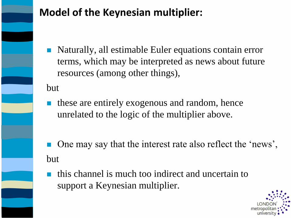
Model of the Keynesian multiplier:
Naturally, all estimable Euler equations contain error
terms, which may be interpreted as news about future
resources (among other things),
but
these are entirely exogenous and random, hence
unrelated to the logic of the multiplier above.
One may say that the interest rate also reflect the „news‟,
but
this channel is much too indirect and uncertain to
support a Keynesian multiplier.

Model of the Keynesian multiplier:To re-instate the multiplier via the effect of news onconsumption, we adopt a variant of the „permanentincome theory of consumption‟, following Obstfeld andRogoff (1996, Ch. 2, equation 2.16).
(1)
Where
,
is the inverse of the discount factor,
At current wealth.
Xt is labour earnings plus monopoly profits, and linearisation gives eq. (2):
0
/)1(~1
~
s
s
tstttt RXEAr
rC
s
v
vt
s
t rR1
)~1(
0
11
0 )~1(
)~1/()1)(1(~1
1
)~1(
)1(~1
~
ss
ststt
ss
stttt
r
yrrE
rr
xEa
r
r
C
Xc

Model of the Keynesian multiplier:
Following Deaton (1990, Ch. 3), we use the period budget
constraint in a beginning-of-period formulation in a
linearised form (eq 3‟):
and supplementing (3‟) into the consumption equation (2):
ttttt rcA
Cx
A
Xara )1()1()~1( 111
0
11
0
111
)~1(
)~1/()1)(1(
1
1
)~1(
)1(
)1()1()~1(
~1
~
ss
ststt
ss
stt
tttt
t
r
yrrE
rr
xE
rcA
Cx
A
Xar
r
r
C
Xc

If we lag (2) and multiply result by (1+r-) and subtract
from (4), we get (5):
Where
• The key is that the evolution of consumption isattributed to „news‟, i.e, revisions of expectations due tothe shocks hitting the system.
• The relation to the multiplier is that when outputchanges, so will profits and labour earnings, and
• this will create „news‟ of higher future earnings,
Model of the Keynesian multiplier:
0
111
0
1
)~1(
)1/()~1/()1()(
~1
)1/()~1/()1(
)~1(
)1)(()1(
~1
~
ss
ststtt
tt
ss
stttt
t
r
yrrEE
r
yrr
r
xEEr
r
r
Cc
sttsttsttt xExExEE 11)(

To close the model, we need:
(6)
where Mt: Real monopolistic (“supernormal”) profits,
in linearised form:
(6‟)
Introducing (6‟) into (5) we get consumption difference (7a)
and present value of labour earnings+monopoly profits Wt:
(7b)
whose revision in expectations form the news effect.
Model of the Keynesian multiplier:
))1/(11()/1( ttttttttt
M
tttt mYLWPMCYLWLWX
p
ttttt lwlshareyx )(
W
r
yrrEEr
r
r
Cc tt
ttttt ~1
)1/()~1/()1()()1(~1
~
1
)1()~1(
)1()1(~1
111
WW tt
tt
t
y
r
rx
r

Fiscal policy and (un-)employment targeting rules
Our second innovation concerns the fiscal policy rule a la
Taylor (1993). I.e. we explicitly recognise that:
fiscal policy is NOT random exogenous shock as wouldhave been modelled customary, and,
it shows endogenous association with the business cycle.
We tested several models based on S&W 2007 model‟sexogenous spending equation but with variations of thenews and/or unemployment* (or the lag-differences ofunemployment or labour force) added on the lines of:
or
*)when if used, the unemployment at time t was defined as adifference between the flexible (frictionless) and the rigideconomy‟s labour forces: ut = lf,t - lt
atygtttutgt guuggg )( 11
atygttttttutgt gEEuuggg W )()( 111

Models:
As a benchmark we used Dynare estimation results of
S&W‟07 model with the original US data and its Log data
density* which is estimated to be -925.087641
M0: A standard Euler equation as in SW, with no news in
either the Euler equation SW or the government spending
„Taylor rule‟, but with the unemployment rate (lagged
difference) defined as above.
We achieved the estimated Log-Density* of -917 , i.e.
substantially higher than for the original S&W 07 model!
*) We used Dynare for estimation of all models to Log data density
[Laplace approximation] stage only at this stage of research.

Models:
M1: Backward looking consumption with news; a
government spending „Taylor rule‟ with news effect:
this model failed the Blanchard-Kahn (1980) test due to
an insufficient number of forward looking variables
tttttt EEcc W )( 11 ,)1()~1(
)1()1(~1
111
WW tt
t
t
t
y
r
rx
r
atygtttttutgt gEEuggg W )( 11

Models:
M2: A standard Euler equation combined with Model 1,
with two types of mutually exclusive (weighted)
heterogeneous agents, one that follow the, the standard
S&W NK forward looking consumption expectation and
the other, backward looking but with the news effect:
This model achieved estimated log-density -915
A similar model but with the forward looking
unemployment difference in the fiscal rule:
achieved even better fit to data with log-density -912!
ttt ccc 21)1( , 10
)()()1( 3121111111 bttttttttt rclElccEcc
tttttt EEcc W )( 11222 ,)1()~1(
)1()1(~1
111
WW tt
t
t
t
y
r
rx
r
atygtttttutgt gEEuggg W )( 11
atygttttttutgt gEEuuggg W )()( 111

Models:
M3: An (SW07) Euler equation with news added, and a
basic government spending rule (I.e. without news or
unemployment targeting rule):
Estimated LDD= -929.6 (which is worse than SW07‟s)
M 4: A standard Euler equation (identical to SW), with a
government spending rule featuring news but no
unemployment targeting rule:
The estimated LDD= -912.1 is indicating importance of
endogenising so called “exogenous” government spending.
)()()()1( 312111 btttttttttttt rclElcEEcEcc W
atygttgt ggg 1
atygtttttgt gEEgg W )( 11

Models:
M5: As Model 4 with the addition of the change in the
unemployment rate in the government spending rule, as
follows:
(usmodel_li1KM01_wgdu.mod ) Estimated LDD=-911.9.
M 6: As model 3 (Euler equation with news) with the
addition of news (but no unemployment) in the fiscal
„Taylor rule‟:
This effectively augments both the Euler equation and the
fiscal rule with news. Estimated LDD=-912.
atygttttttutgt gEEuuggg W )()( 111
)()()()1( 312111 btttttttttttt rclElcEEcEcc W
atygtttttgt gEEgg W )( 11

Models:
M 7: As Model 6 with the addition of the forward-looking
difference in unemployment in the fiscal rule:
Estimated LDD=-911.9
M8: As in model 7 Euler with backward-looking (instead
of forward-looking) change in unemployment in the fiscal
rule:
Estimated LDD=-912.3; estimated 0.4395.
)()()()1( 312111 btttttttttttt rclElcEEcEcc W
atygttttttutgt gEEuuggg W )()( 111
)()()()1( 312111 btttttttttttt rclElcEEcEcc W
atygttttttutgt gEEuuggg W )()( 111

Models:
M 9: As in models 8 and 9 with the simple unemployment
rate (instead of its difference) in the fiscal unemployment
targeting rule:
Estimated LDD=-911.5, 0.45
M 11: As in model 9 but with backward-looking change in
labour force instead of unemployment in the fiscal rule:
Estimated LDD=-910.5;
M 12: A similar model but with no news in either Euler or
fiscal rule but only labour difference gives LLD=-913.1
)()()()1( 312111 btttttttttttt rclElcEEcEcc W
atygttttttutgt gEEuuggg W )()( 111
atygttttttutgt gEEllggg W )()( 111

Results:Multiplier Fiscal policy
Rank Model
news
in c
news
in g
(un)emp
rule
used
unempl
oyment
params LDD
MCMC
10000 Note
1 11 0.1463 -0.26 lab bk dif -0.1732 -910.513
2 9 0.1634 -0.298 simple u 0.0265 -911.493
3 7 0.151 -0.281 u fwd dif 0.164 -911.918
4 5 -0.259 u bk dif 0.1592 -911.926
5 6 0.1569 -0.295 -912.057
6 4 -0.316 -912.079
7 8 0.1544 -0.265 u bk dif 0.1154 -912.331
8 10 0.269 -0.261 simple u 0.0257 -912.352 Heterogen agents
9 12 lab bk dif -0.4711 -913.115 -917.586
10 2 0.4602 -0.318 simple u 0.0218 -915.805 Heterogen agents
11 0 u bk dif 0.4802 -917.623 -921.946
12 SW1 -924.956 -929.036 SW 07 li1
13 SW2 -925.088 -929.985
SW 07 li2,
ORIGINAL
14 3 -0.024 -929.619

Original S&W 2007 model responses to hg shock to g (I.e. g)
Results:
5 10 15 20-1
0
1dy
5 10 15 200
0.5
1y
5 10 15 200
0.01
0.02pinfobs
5 10 15 200
0.02
0.04robs
5 10 15 20-0.4
-0.2
0c
5 10 15 20-0.05
0
0.05w
5 10 15 200
0.2
0.4lab
5 10 15 200
0.5
1g
5 10 15 20-1
-0.5
0inve

Results:
The employment difference based fiscal rule only model 12 responses to
hg shock to g (I.e. g)

News and fiscal rule model 11 responses to hg shock to g (I.e. g)
Results:

Results (I):
• Experimenting with the models and data in the “linear
space” experimental laboratory of DSGE models
estimation and simulation Dynare toolkit, we found that
• our model behaves in a comparable manner to SW07.
• Having, however, with a sizeably higher likelihood, our
models provide a much better fit to data than SW07.
• Our estimation results show dramatic improvements
when either one or both factors,
– the news, and/or
– the (un-) employment
targeting rules are added to the so called “exogenous”
(government) spending and making it more endogenous.

The Multipliers
• Textbook multiplier: (Yt-Y0)/dG0
• 2 adjustments to render meaningful:
• As raw IRF of consumption gives a deviation of c from
its trend as a % of C, we multiply by the mean
consumption-output ratio (0.6) to express deviations as
% of output;
• Question over „true‟ exogeneity: In our model it is the
shock (eg) but if government have a target of g, then the
latter may be thought of as the exogenous variable with
eg as residual (endogenous) adjustment – hence, take
either as the true fiscal impulse.

The Multipliers – Table 2
Table 2 presents the following multipliers:
The models are organised in pairs, where, in each pair,
• Model a is the version with news in the Euler equation,
• Model b is the version of the same model without news*
*) Models 2a and 2b are not exact counterparts, in this respect, as 2a has
unemployment in the fiscal rule, whereas 2b has the difference in
unemployment in the fiscal rule; otherwise, they are exact counterparts,
except that 2a has news in the Euler equation whereas 2b does not.)

Table 2 – part i.
Quarter after shock
0 1 2 3 4 5 6 7 11 15 19
1a. usmodel_li1KM01_wswgdl_1_ news in SW+ g + lab diff in g LDD -910 BEST of all
c_eg/eg 0.16 0.10 0.05 0.01 -0.03 -0.05 -0.08 -0.10 -0.14 -0.16 -0.17
y_eg/eg 0.80 0.69 0.60 0.53 0.47 0.41 0.37 0.33 0.23 0.18 0.15
g_eg/eg 0.60 0.60 0.59 0.59 0.58 0.57 0.56 0.55 0.51 0.46 0.42
c_eg/g0 0.26 0.17 0.08 0.01 -0.04 -0.09 -0.13 -0.16 -0.24 -0.27 -0.28
y_eg/g0 1.34 1.16 1.01 0.88 0.78 0.69 0.61 0.55 0.39 0.30 0.24
g_eg/g0 1.00 1.00 0.99 0.98 0.97 0.95 0.94 0.92 0.84 0.77 0.69
1b. usmodel_lik1_gl_1 no news only diff lab in g LDD -913
c_eg/eg -0.03 -0.07 -0.10 -0.12 -0.14 -0.16 -0.17 -0.18 -0.20 -0.21 -0.20
y_eg/eg 0.74 0.66 0.59 0.54 0.48 0.44 0.40 0.37 0.27 0.21 0.17
g_eg/eg 0.74 0.74 0.74 0.74 0.73 0.72 0.71 0.70 0.63 0.57 0.51
c_eg/g0 -0.05 -0.09 -0.13 -0.16 -0.19 -0.21 -0.23 -0.24 -0.27 -0.28 -0.27
y_eg/g0 0.99 0.89 0.80 0.72 0.65 0.59 0.54 0.49 0.36 0.28 0.22
g_eg/g0 1.00 1.00 1.00 1.00 0.99 0.97 0.96 0.94 0.86 0.77 0.68

Table 2 – part ii.
Quarter after shock
0 1 2 3 4 5 6 7 11 15 19
2a. usmodel_li1KM01_swcy1gu_w1_rc1pi2_ news in SW+ g + u in g LL911 BEST with unemployment
c_eg/eg 0.20 0.14 0.09 0.05 0.01 -0.02 -0.05 -0.07 -0.13 -0.15 -0.16
y_eg/eg 0.86 0.72 0.60 0.51 0.43 0.36 0.30 0.26 0.15 0.09 0.07
g_eg/eg 0.62 0.60 0.57 0.55 0.53 0.51 0.49 0.48 0.42 0.37 0.33
c_eg/g0 0.33 0.23 0.15 0.08 0.02 -0.03 -0.07 -0.11 -0.20 -0.24 -0.26
y_eg/g0 1.39 1.16 0.97 0.81 0.68 0.58 0.49 0.42 0.24 0.15 0.11
g_eg/g0 1.00 0.96 0.92 0.88 0.85 0.82 0.79 0.76 0.67 0.59 0.52
2b. usmodel_li1KM01_wgdu _no news in SW but news and du in g 911.9
c_eg/eg -0.02 -0.05 -0.07 -0.09 -0.11 -0.12 -0.13 -0.14 -0.16 -0.16 -0.16
y_eg/eg 0.73 0.64 0.56 0.49 0.44 0.39 0.35 0.32 0.23 0.18 0.14
g_eg/eg 0.72 0.70 0.67 0.66 0.64 0.62 0.60 0.59 0.52 0.46 0.41
c_eg/g0 -0.03 -0.07 -0.10 -0.13 -0.15 -0.17 -0.19 -0.20 -0.22 -0.22 -0.22
y_eg/g0 1.02 0.89 0.78 0.68 0.61 0.54 0.49 0.45 0.32 0.25 0.20
g_eg/g0 1.00 0.96 0.93 0.91 0.88 0.86 0.84 0.82 0.73 0.64 0.57

Table 2 – Model 1a: responses normalised by eg0

Table 2 – Model 1a : responses normalised by g0

Multipliers – cont’d.
• Furthermore, the numerator of the multiplier, (Yt-Y0)/dG0,
can be decomposed as change along the trend plus
deviation from it;
• Only latter should be considered:
• Trend is completely exogenous, unrelated to fiscal
policy (as that is not assumed productive);
• Trend explodes asymptotically;
• Hence, if output devs. (in levels) is and
it follows that .
• Table 3 presents

Table 3
Quarter after shock
0 1 2 3 4 5 6 7 11 15 19
1a. usmodel_li1KM01_wswgdl_1_ news in SW+ g + lab diff in g LDD -910 BEST of all
c_eg/eg 0.16 0.10 0.05 0.01 -0.03 -0.06 -0.08 -0.10 -0.15 -0.17 -0.18
y_eg/eg 0.80 0.70 0.61 0.54 0.47 0.42 0.38 0.34 0.24 0.19 0.16
g_eg/eg 0.60 0.60 0.60 0.60 0.59 0.58 0.58 0.57 0.53 0.49 0.45
c_eg/g0 0.26 0.17 0.08 0.01 -0.04 -0.09 -0.13 -0.17 -0.25 -0.29 -0.31
y_eg/g0 1.34 1.16 1.02 0.89 0.79 0.70 0.63 0.57 0.41 0.32 0.26
g_eg/g0 1.00 1.00 1.00 0.99 0.98 0.97 0.96 0.95 0.88 0.82 0.75
1b. usmodel_lik1_gl_1 no news only diff lab in g LDD -913
c_eg/eg -0.03 -0.07 -0.10 -0.12 -0.14 -0.16 -0.18 -0.19 -0.21 -0.22 -0.22
y_eg/eg 0.74 0.67 0.60 0.54 0.49 0.45 0.41 0.38 0.28 0.22 0.18
g_eg/eg 0.74 0.75 0.75 0.75 0.75 0.74 0.73 0.72 0.67 0.61 0.55
c_eg/g0 -0.05 -0.09 -0.13 -0.17 -0.20 -0.22 -0.24 -0.25 -0.28 -0.30 -0.30
y_eg/g0 0.99 0.90 0.81 0.73 0.66 0.60 0.55 0.51 0.38 0.30 0.24
g_eg/g0 1.00 1.01 1.01 1.01 1.00 0.99 0.98 0.97 0.90 0.82 0.74

Table 3 – Model a: responses normalised by eg0

Table 3 – Model a: responses normalised by g0

Results (II):
1. Models with news in the Euler equation consistently
show higher responses of both consumption and output
to the fiscal shock.
2. Choice of the scaling factor (one standard deviation of
the estimated exogenous spending shock or g0) matters a
lot. In the latter case, we get true Keynesian multipliers
of higher than unity, that last at least for a year.
3. Incorporation of news is also critical in the sense that,
with it, consumption responds positively to the fiscal
shock in both types of shock (eg0 and g0), whereas
4. without it, the consumption response is lower, and
negative in the case of the former type of shock.
This refutes the key criticism of the fiscal multiplier that it
crowds out private consumption (if it actually does)
view (see e.g. Barro, 2010)

This paper seeks to enhance our understanding of fiscal policy in
the context of the
business cycles and current crisis, and
its potential for stabilisation.
We utilise a standard medium-sized DSGE model as in Smets
and Wouters (2007) (see also Drautzburg and Uhlig, 2010).
Our innovation is twofold,
to incorporate a Keynesian multiplier by allowing for „news‟
(unexpected revisions in lifetime wealth) to augment the
Euler equation, hence giving rise to an output news –
consumption – further output changes virtuous circle; and
to account for the evolution of fiscal policy that is not random
and exogenous, but may follow a rule akin to that of Taylor
(1993) for monetary policy.
Conclusions (I):

Conclusions (II):
• Another (New) Keynesian feature is inclusion of change
of employment rates or of unemployment (as difference
between the employment rates of the actual and flexible-
price economy) that affects the fiscal policy rule.
• More neo-classical features include
– intertemporal optimisation,
– elastic labour supply,
– trend growth.
• Our results show dramatic improvements in estimationresults over the standard SW specification.
The „news‟ channel allows for a change in resultstowards a more „keynesian‟ flavour – more prolongedoutput responses, positive consumption responses.

Possible extensions in future work:
• Extend the model towards heterogeneous framework, e.g. add the non-Ricardian consumers a la Drautzburg and Uhlig,
• optimistic and pessimistic (Animal spirit driven) agents along the lines of DeGrauwe, (2009) and
• the imperfect (partial) information solution framework with the adaptive behaving agents on the lines of Levine, Pearlman, Perendia and Yung (2010).
• Allow for beneficial effects of public debt on growth (e.g., Traum and Yang, 2009) – e.g., due to a possible reduction in capital gains taxes or increase in business investment.
• Allow for special nature of government spending:
• production-enhancing, e.g. via infrastructure-building;
• related to defence (see papers by Barro).

Thank you for listening!
The Keynesian multiplier, news and fiscal policy rules in a DSGE model
Authors:
George Perendia and Dr Chris [email protected] [email protected]
London Metropolitan University