Embed Size (px)
Citation preview

Introduction Main results Ancilliary results Conclusion
The kinks of financial journalism
Diego Garcı́aUniversity of Colorado Boulder
2nd Annual News & Finance conferenceColumbia University
March 8th, 2017
Diego Garcı́a (2017), CU-Boulder The kinks of financial journalism 1 / 36
Introduction Main results Ancilliary results Conclusion
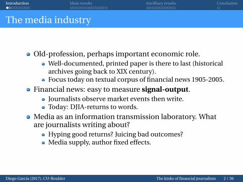
The media industry
Old-profession, perhaps important economic role.Well-documented, printed paper is there to last (historicalarchives going back to XIX century).Focus today on textual corpus of financial news 1905-2005.
Financial news: easy to measure signal-output.Journalists observe market events then write.Today: DJIA-returns to words.
Media as an information transmission laboratory. Whatare journalists writing about?
Hyping good returns? Juicing bad outcomes?Media supply, author fixed effects.
Diego Garcı́a (2017), CU-Boulder The kinks of financial journalism 2 / 36
Introduction Main results Ancilliary results Conclusion
Literature review
Politics slant: media can taint voters.Gentzkow and Shapiro (2006, 2010, 2011).DellaVigna and Kaplan (2007).
In finance: media can effect asset prices.Shiller (2000), Tetlock (2007), Garcı́a (2013).Engelberg and Parsons (2011), Dougal et al. (2012).Reuters and Zitzewitz (2006).
Literature focus: media drives economic variables.But what drives financial media slant?
This paper’s premise: the media itself is an interestingeconomic agent.Financial journalists get to colour Wall Street, but how?
Diego Garcı́a (2017), CU-Boulder The kinks of financial journalism 3 / 36

Introduction Main results Ancilliary results Conclusion
Theories? No theories
Two (non exclusive) interpretations of the data:1 Words are a reflection of journalists’
preferences/incentives (supply side).Maximize attention of readers.“Hyping” to sell more newspapers.
2 Journalists catering to investors (demand driven).Informational role: tell investors important news.Confirmation biases: journalists write what investors wantto read.
Demand and supply stories obviously intertwined.
Diego Garcı́a (2017), CU-Boulder The kinks of financial journalism 4 / 36
Introduction Main results Ancilliary results Conclusion
Null hypothesis
What type of slanting maximizes attention?
1 Informational role would probably argue for emphasizingbig stock price movements (important days).
2 Attention theories can rationalize emphasis on positivedomain, and/or on average days.
Leading null hypothesis:1 Linear relationship between signals and words.
Natural null.As in Admati and Pfleiderer (1986, 1987).
2 Shiller’s entertainment role hypothesis.“Hyping” big positive returns.“Exaggerate” average days.
Diego Garcı́a (2017), CU-Boulder The kinks of financial journalism 5 / 36
Introduction Main results Ancilliary results Conclusion
The paper in a nutshell
Large scale study of the content of financial news as afunction of market movements.
Little documented in the literature.Tetlock (2007) and Garcı́a (2013) show that they use morepositive/less negative words when market goes up.
Focus on lagged market returns, the “signal” that they arewriting about (noisy proxy, DJIA returns).
t-day lags.More unusual variables (not in draft).
Empirical approach: non-linear fit of media content as afunction of lagged market (DJIA) returns.
Diego Garcı́a (2017), CU-Boulder The kinks of financial journalism 6 / 36
Introduction Main results Ancilliary results Conclusion
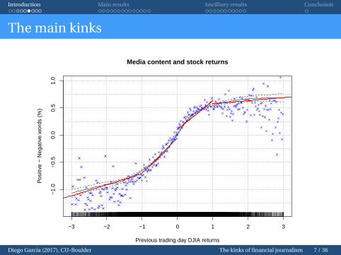
The main kinks
−3 −2 −1 0 1 2 3
−1.
0−
0.5
0.0
0.5
1.0
Media content and stock returns
Previous trading day DJIA returns
Pos
itive
− N
egat
ive
wor
ds (
%)
Diego Garcı́a (2017), CU-Boulder The kinks of financial journalism 7 / 36
Introduction Main results Ancilliary results Conclusion
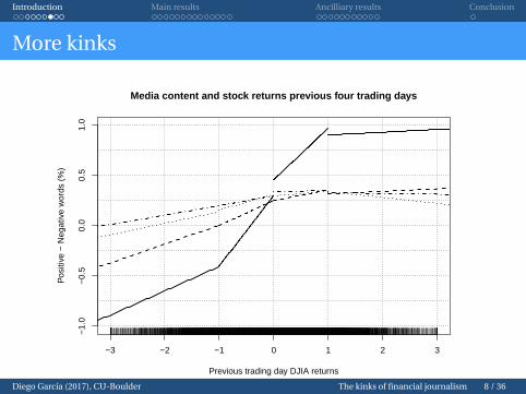
More kinks
−3 −2 −1 0 1 2 3
−1.
0−
0.5
0.0
0.5
1.0
Media content and stock returns previous four trading days
Previous trading day DJIA returns
Pos
itive
− N
egat
ive
wor
ds (
%)
Diego Garcı́a (2017), CU-Boulder The kinks of financial journalism 8 / 36
Introduction Main results Ancilliary results Conclusion
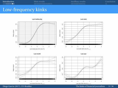
Low-frequency kinks
−3 −2 −1 0 1 2 3
−1.
0−
0.5
0.0
0.5
Last trading day
Last trading day DJIA return Rt
Med
ia c
onte
nt
−3 −2 −1 0 1 2 3
−0.
6−
0.4
−0.
20.
00.
2
Last week
Last week DJIA return Rt−4,t−1
Med
ia c
onte
nt
−3 −2 −1 0 1 2 3
−0.
4−
0.3
−0.
2−
0.1
0.0
0.1
0.2
Last month
Last month DJIA return Rt−24,t−5
Med
ia c
onte
nt
−3 −2 −1 0 1 2 3
−0.
20.
00.
20.
4
Last year
Last year DJIA return Rt−252,t−25
Med
ia c
onte
nt
Diego Garcı́a (2017), CU-Boulder The kinks of financial journalism 9 / 36
Introduction Main results Ancilliary results Conclusion
The new facts
There is an economically large kink in the domains ofgains/losses.
No difference in content when DJIA is 1% or when it is 3%,significant differences between−1% and−3%.
Convex in domain of losses, concave in domain of gains.S-shaped non-linear fit.
Persistence of effect over several days.News load on negative returns, but not on positivereturns.
Diego Garcı́a (2017), CU-Boulder The kinks of financial journalism 10 / 36

Introduction Main results Ancilliary results Conclusion
The data
Standard finance/macro variables (DJIA, CRSP).Word counts from NYT and WSJ (1905–2005).
“Financial Markets” and “Topics in Wall Street” from NYT.“Abreast of the market” from WSJ.
Aggregate articles by “trading clock”.Assume things are published between trading dates,irrespective of when.Saturday versus Sunday versus Monday, and holidayweekday issues.
Media content definition: percent of positive wordsminus negative words in articles.
Data calls for dictionary approach.Loughran-McDonald dictionaries.
Diego Garcı́a (2017), CU-Boulder The kinks of financial journalism 11 / 36
Introduction Main results Ancilliary results Conclusion
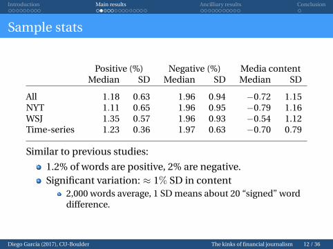
Sample stats
Positive (%) Negative (%) Media contentMedian SD Median SD Median SD
All 1.18 0.63 1.96 0.94 −0.72 1.15NYT 1.11 0.65 1.96 0.95 −0.79 1.16WSJ 1.35 0.57 1.96 0.93 −0.54 1.12Time-series 1.23 0.36 1.97 0.63 −0.70 0.79
Similar to previous studies:
1.2% of words are positive, 2% are negative.Significant variation: ≈ 1% SD in content
2,000 words average, 1 SD means about 20 “signed” worddifference.
Diego Garcı́a (2017), CU-Boulder The kinks of financial journalism 12 / 36
Introduction Main results Ancilliary results Conclusion
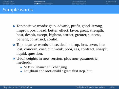
Sample words
Top positive words: gain, advanc, profit, good, strong,improv, posit, lead, better, effect, favor, great, strength,best, despit, except, highest, attract, greater, success,benefit, construct, confid.
Top negative words: close, declin, drop, loss, sever, late,lost, concern, cost, cut, weak, poor, eas, contract, sharpli,liquid, question.tf-idf weights in new version, plus non-parametricmethods.
NLP in Finance still changing.Loughran and McDonald a great first step, but.
Diego Garcı́a (2017), CU-Boulder The kinks of financial journalism 13 / 36
Introduction Main results Ancilliary results Conclusion
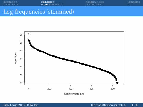
Log-frequencies (stemmed)
●●●
●●
●●●●●●●●●●●●●●●●●●●●●●●●●●●●●●●●●●●●●●●●●●●●●●●●●●●●●●●●●●●●●●●●●●●●●●●●●●●●●●●●●●●●●●●●●●●●●●●●●●●●●●●●●●●●●●●●●●●●●●●●●●●●●●●●●●●●●●●●●●●●●●●●●●●●●●●●●●●●●●●●●●●●●●●●●●●●●●●●●●●●●●●●●●●●●●●●●●●●●●●●●●●●●●●●●●●●●●●●●●●●●●●●●●●●●●●●●●●●●●●●●●●●●●●●●●●●●●●●●●●●●●●●●●●●●●●●●●●●●●●●●●●●●●●●●●●●●●●●●●●●●●●●●●●●●●●●●●●●●●●●●●●●●●●●●●●●●●●●●●●●●●●●●●●●●●●●●●●●●●●●●●●●●●●●●●●●●●●●●●●●●●●●●●●●●●●●●●●●●●●●●●●●●●●●●●●●●●●●●●●●●●●●●●●●●●●●●●●●●●●●●●●●●●●●●●●●●●●●●●●●●●●●●●●●●●●●●●●●●●●●●●●●●●●●●●●●●●●●●●●●●●●●●●●●●●●●●●●●●●●●●●●●●●●●●●●●●●●●●●●●●●●●●●●●●●●●●●●●●●●●●●●●●●●●●●●●●●●●●●●●●●●●●●●●●●●●●●●●●●●●●●●●●●●●●●●●●●●●●●●●●●●●●●●●●●●●●●●●●●●●●●●●●●●●●●●●●●●●●●●●●●●●●●●●●●●●●●●●●●●●●●●●●●●●●●●●●●●●●●●●●●●●●●●●●●●●●●●●●●●●●●●●●●●●●●●●●●●●●●●●●●●●●●●●●●●●●●●●●●●●●●●●●●●●●●●●●●●●●●●●●●●●●●●●●●●●●●●●●●●●●●●●●●●●●●●●●●●●●●●●●
●●●●●
●●●●●●
●●●●●●●●●●●
0 200 400 600 800
02
46
810
12
Negative words (LM)
Fre
quen
cies
Diego Garcı́a (2017), CU-Boulder The kinks of financial journalism 14 / 36
Introduction Main results Ancilliary results Conclusion
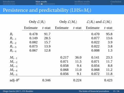
Persistence and predictability (LHS=Mt )
Only L(Rt ) Only L(Mt ) L(Rt ) and L(Mt )
Estimate t-stat Estimate t-stat Estimate t-stat
Rt 0.478 91.7 0.470 95.8Rt−1 0.149 28.5 0.077 13.6Rt−2 0.082 15.7 0.022 3.9Rt−3 0.073 13.9 0.022 3.8Rt−4 0.067 12.8 0.008 1.3
Mt−1 0.217 36.0 0.141 23.3Mt−2 0.071 11.5 0.071 11.7Mt−3 0.058 9.4 0.054 8.8Mt−4 0.068 11.0 0.068 11.2Mt−5 0.056 9.1 0.072 11.8
adj-R2 0.346 0.224 0.423
Diego Garcı́a (2017), CU-Boulder The kinks of financial journalism 15 / 36
Introduction Main results Ancilliary results Conclusion
Econometric specification
Main specification
Mt = f (Rt ;α, β) + ηXt + εt ;
Mt is media content published on date t + 1 (written inthe afternoon of time t).
Rt is the log-return on DJIA from closing of date t − 1 toclosing of date t , censored at±3%.
Controls Xt include L(Rt ), L(Mt ), time-spline, monthdummies, day-of-the-week dummies.
Standard errors Newey-West with 10 lags (HAC or OLSwork too).
Diego Garcı́a (2017), CU-Boulder The kinks of financial journalism 16 / 36
Introduction Main results Ancilliary results Conclusion
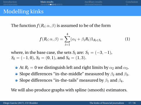
Modelling kinks
The function f (Rt ;α, β) is assumed to be of the form
f (Rt ;α, β) =
4∑i=1
(αi + βiRt )1Rt∈Si (1)
where, in the base case, the sets Si are: S1 = (−3,−1),S2 = (−1, 0), S3 = (0, 1), and S4 = (1, 3).
At Rt = 0 we distinguish left and right limits by α2 and α3.
Slope differences “in-the-middle” measured by β2 and β3.
Slope differences “in-the-tails” measured by β1 and β4.
We will also produce graphs with spline (smooth) estimators.
Diego Garcı́a (2017), CU-Boulder The kinks of financial journalism 17 / 36
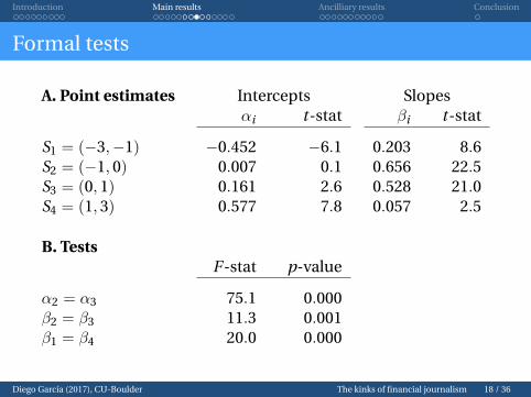
Introduction Main results Ancilliary results Conclusion
Formal tests
A. Point estimates Intercepts Slopesαi t-stat βi t-stat
S1 = (−3,−1) −0.452 −6.1 0.203 8.6S2 = (−1, 0) 0.007 0.1 0.656 22.5S3 = (0, 1) 0.161 2.6 0.528 21.0S4 = (1, 3) 0.577 7.8 0.057 2.5
B. TestsF -stat p-value
α2 = α3 75.1 0.000β2 = β3 11.3 0.001β1 = β4 20.0 0.000
Diego Garcı́a (2017), CU-Boulder The kinks of financial journalism 18 / 36
Introduction Main results Ancilliary results Conclusion
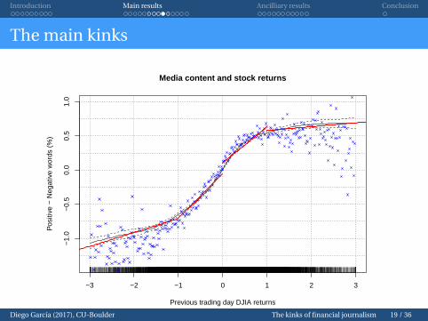
The main kinks
−3 −2 −1 0 1 2 3
−1.
0−
0.5
0.0
0.5
1.0
Media content and stock returns
Previous trading day DJIA returns
Pos
itive
− N
egat
ive
wor
ds (
%)
Diego Garcı́a (2017), CU-Boulder The kinks of financial journalism 19 / 36
Introduction Main results Ancilliary results Conclusion
Main findings
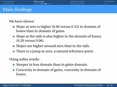
We have shown:
Slope at zero is higher (0.66 versus 0.53) in domain oflosses than in domain of gains.
Slope at the tails is also higher in the domain of losses(0.20 versus 0.06).
Slopes are higher around zero than in the tails.
There is a jump at zero, a natural reference point.
Using softer words:
Steeper in loss domain than in gains domain.
Concavity in domain of gains, convexity in domain oflosses.
Diego Garcı́a (2017), CU-Boulder The kinks of financial journalism 20 / 36
Introduction Main results Ancilliary results Conclusion
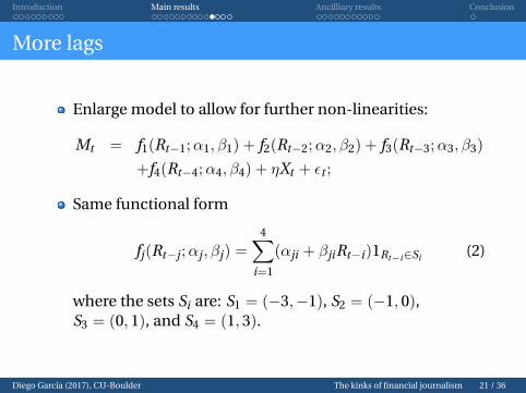
More lags
Enlarge model to allow for further non-linearities:
Mt = f1(Rt−1;α1, β1) + f2(Rt−2;α2, β2) + f3(Rt−3;α3, β3)
+f4(Rt−4;α4, β4) + ηXt + εt ;
Same functional form
fj(Rt−j ;αj , βj) =
4∑i=1
(αji + βjiRt−i)1Rt−i∈Si (2)
where the sets Si are: S1 = (−3,−1), S2 = (−1, 0),S3 = (0, 1), and S4 = (1, 3).
Diego Garcı́a (2017), CU-Boulder The kinks of financial journalism 21 / 36
Introduction Main results Ancilliary results Conclusion
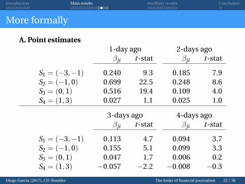
More formally
A. Point estimates1-day ago 2-days agoβji t-stat βji t-stat
S1 = (−3,−1) 0.240 9.3 0.185 7.9S2 = (−1, 0) 0.699 22.5 0.248 8.6S3 = (0, 1) 0.516 19.4 0.109 4.0S4 = (1, 3) 0.027 1.1 0.025 1.0
3-days ago 4-days agoβji t-stat βji t-stat
S1 = (−3,−1) 0.113 4.7 0.094 3.7S2 = (−1, 0) 0.155 5.1 0.099 3.3S3 = (0, 1) 0.047 1.7 0.006 0.2S4 = (1, 3) −0.057 −2.2 −0.008 −0.3
Diego Garcı́a (2017), CU-Boulder The kinks of financial journalism 22 / 36

Introduction Main results Ancilliary results Conclusion
More kinks
−3 −2 −1 0 1 2 3
−1.
0−
0.5
0.0
0.5
1.0
Media content and stock returns previous four trading days
Previous trading day DJIA returns
Pos
itive
− N
egat
ive
wor
ds (
%)
Diego Garcı́a (2017), CU-Boulder The kinks of financial journalism 23 / 36
Introduction Main results Ancilliary results Conclusion
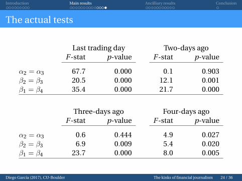
The actual tests
Last trading day Two-days agoF -stat p-value F -stat p-value
α2 = α3 67.7 0.000 0.1 0.903β2 = β3 20.5 0.000 12.1 0.001β1 = β4 35.4 0.000 21.7 0.000
Three-days ago Four-days agoF -stat p-value F -stat p-value
α2 = α3 0.6 0.444 4.9 0.027β2 = β3 6.9 0.009 5.4 0.020β1 = β4 23.7 0.000 8.0 0.005
Diego Garcı́a (2017), CU-Boulder The kinks of financial journalism 24 / 36
Introduction Main results Ancilliary results Conclusion
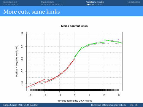
Robustness, interpretation, mechanism
Different econometric specifications.More cuts.Other indexes.
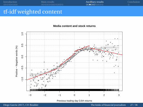
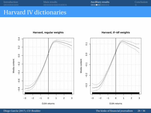
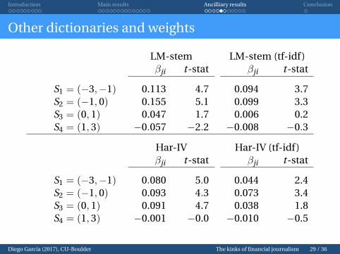
Different NLP techniques.Harvard versus LM dictionaries.tf-idf weights.Positive versus negative word lists.
Possible mechanisms (demand/supply).Time-series variation.Author-fixed effects.
Diego Garcı́a (2017), CU-Boulder The kinks of financial journalism 25 / 36
Introduction Main results Ancilliary results Conclusion
More cuts, same kinks
−3 −2 −1 0 1 2 3
−1.
0−
0.5
0.0
0.5
1.0
Media content kinks
Previous trading day DJIA returns
Pos
itive
− n
egat
ive
wor
ds (
%)
Diego Garcı́a (2017), CU-Boulder The kinks of financial journalism 26 / 36
Introduction Main results Ancilliary results Conclusion
tf-idf weighted content
−3 −2 −1 0 1 2 3
−1.
0−
0.5
0.0
0.5
1.0
Media content and stock returns
Previous trading day DJIA returns
Pos
itive
− N
egat
ive
wor
ds (
%)
Diego Garcı́a (2017), CU-Boulder The kinks of financial journalism 27 / 36
Introduction Main results Ancilliary results Conclusion
Harvard IV dictionaries
−3 −2 −1 0 1 2 3
−0.
8−
0.6
−0.
4−
0.2
0.0
0.2
0.4
Harvard, regular weights
DJIA returns
Med
ia c
onte
nt
−3 −2 −1 0 1 2 3
−0.
3−
0.2
−0.
10.
00.
1
Harvard, tf−idf weights
DJIA returns
Med
ia c
onte
nt
Diego Garcı́a (2017), CU-Boulder The kinks of financial journalism 28 / 36
Introduction Main results Ancilliary results Conclusion
Other dictionaries and weights
LM-stem LM-stem (tf-idf)βji t-stat βji t-stat
S1 = (−3,−1) 0.113 4.7 0.094 3.7S2 = (−1, 0) 0.155 5.1 0.099 3.3S3 = (0, 1) 0.047 1.7 0.006 0.2S4 = (1, 3) −0.057 −2.2 −0.008 −0.3
Har-IV Har-IV (tf-idf)βji t-stat βji t-stat
S1 = (−3,−1) 0.080 5.0 0.044 2.4S2 = (−1, 0) 0.093 4.3 0.073 3.4S3 = (0, 1) 0.091 4.7 0.038 1.8S4 = (1, 3) −0.001 −0.0 −0.010 −0.5
Diego Garcı́a (2017), CU-Boulder The kinks of financial journalism 29 / 36
Introduction Main results Ancilliary results Conclusion
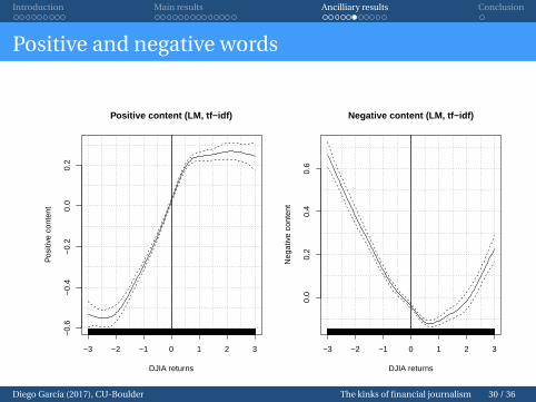
Positive and negative words
−3 −2 −1 0 1 2 3
−0.
6−
0.4
−0.
20.
00.
2
Positive content (LM, tf−idf)
DJIA returns
Pos
itive
con
tent
−3 −2 −1 0 1 2 3
0.0
0.2
0.4
0.6
Negative content (LM, tf−idf)
DJIA returns
Neg
ativ
e co
nten
t
Diego Garcı́a (2017), CU-Boulder The kinks of financial journalism 30 / 36
Introduction Main results Ancilliary results Conclusion
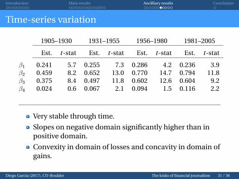
Time-series variation
1905–1930 1931–1955 1956–1980 1981–2005
Est. t-stat Est. t-stat Est. t-stat Est. t-stat
β1 0.241 5.7 0.255 7.3 0.286 4.2 0.236 3.9β2 0.459 8.2 0.652 13.0 0.770 14.7 0.794 11.8β3 0.375 8.4 0.497 11.8 0.602 12.6 0.604 9.2β4 0.024 0.6 0.067 2.1 0.094 1.5 0.116 2.2
Very stable through time.
Slopes on negative domain significantly higher than inpositive domain.
Convexity in domain of losses and concavity in domain ofgains.
Diego Garcı́a (2017), CU-Boulder The kinks of financial journalism 31 / 36

Introduction Main results Ancilliary results Conclusion
Author fixed-effects
Estimates for each author of AOTM colum (WSJ), 1970–2005.
β1 β2 β3 β4
N Estimate t-stat Estimate t-stat Estimate t-stat Estimate t-statHillery 2413 0.333 3.3 0.871 9.3 0.636 6.5 0.113 1.3Obrien 1215 0.533 3.5 1.169 5.1 1.069 5.2 0.218 1.5Talley 915 −0.025 −0.1 1.111 5.4 1.097 5.3 −0.258 −1.3Marcial 625 0.899 2.3 0.430 1.5 0.830 2.8 −0.169 −0.5Garcia 588 0.289 1.4 1.469 6.1 0.597 2.7 −0.112 −0.7Smith 302 −0.246 −0.6 1.124 3.7 0.945 3.0 −0.078 −0.3Wilson 251 0.037 0.1 0.988 2.9 0.656 2.4 0.397 1.3Browning 250 0.592 1.6 0.156 0.4 0.198 0.5 −0.066 −0.2Pettit 222 0.307 0.4 1.313 3.6 0.218 0.5 −0.587 −0.4Sease 157 0.624 1.8 0.735 1.6 −0.017 −0.0 0.648 0.8
Kinks pervasive for all authors.
Slopes on negative domain significantly higher than in positivedomain.
Convexity in domain of losses and concavity in domain ofgains.
Diego Garcı́a (2017), CU-Boulder The kinks of financial journalism 32 / 36
Introduction Main results Ancilliary results Conclusion
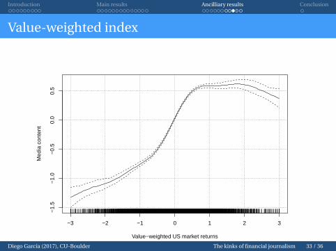
Value-weighted index
−3 −2 −1 0 1 2 3
−1.
5−
1.0
−0.
50.
00.
5
Value−weighted US market returns
Med
ia c
onte
nt
Diego Garcı́a (2017), CU-Boulder The kinks of financial journalism 33 / 36
Introduction Main results Ancilliary results Conclusion
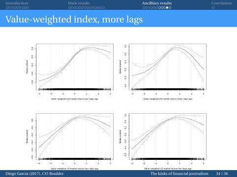
Value-weighted index, more lags
−3 −2 −1 0 1 2 3
−0.
6−
0.4
−0.
20.
00.
2
Value−weighted US market returns two−days ago
Med
ia c
onte
nt
−3 −2 −1 0 1 2 3
−0.
4−
0.3
−0.
2−
0.1
0.0
0.1
Value−weighted US market returns three−days ago
Med
ia c
onte
nt
−3 −2 −1 0 1 2 3
−0.
5−
0.4
−0.
3−
0.2
−0.
10.
0
Value−weighted US market returns four−days ago
Med
ia c
onte
nt
−3 −2 −1 0 1 2 3
−0.
5−
0.4
−0.
3−
0.2
−0.
10.
00.
1
Value−weighted US market returns five−days ago
Med
ia c
onte
nt
Diego Garcı́a (2017), CU-Boulder The kinks of financial journalism 34 / 36

Introduction Main results Ancilliary results Conclusion
Summary
Number of cuts does not affect any conclusions.Even smooth estimators tell the same story.
Results for value-weighted index are even stronger.If I were smarter I would redo main tables with KenFrench’s index.
Differences in domain of gains and losses shows up witheven (very) long lags.
Returns in days 1–4 move media content a fair amount,but only on the negative domain.Returns in days 6–25 move media content a little, but onlyon the negative domain.
Demand versus supply theories.Time-series stability and author-fixed effects suggestive ofkinks coming from demand side.
Diego Garcı́a (2017), CU-Boulder The kinks of financial journalism 35 / 36
Introduction Main results Ancilliary results Conclusion
Conclusion
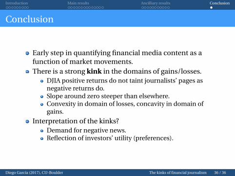
Early step in quantifying financial media content as afunction of market movements.There is a strong kink in the domains of gains/losses.
DJIA positive returns do not taint journalists’ pages asnegative returns do.Slope around zero steeper than elsewhere.Convexity in domain of losses, concavity in domain ofgains.
Interpretation of the kinks?Demand for negative news.Reflection of investors’ utility (preferences).
Diego Garcı́a (2017), CU-Boulder The kinks of financial journalism 36 / 36
Weather and calendar effects
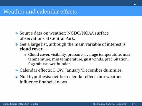
Source data on weather: NCDC/NOAA surfaceobservations at Central Park.Get a large list, although the main variable of interest iscloud cover.
Cloud cover, visibility, pressure, average temperature, maxtemperature, min temperature, gust winds, precipitation,fog/rain/snow/thunder.
Calendar effects: DOW, January/December dummies.
Null hypothesis: neither calendar effects nor weatherinfluence financial news.
Diego Garcı́a (2017), CU-Boulder The kinks of financial journalism 1 / 4
Weather variables
lm rlm
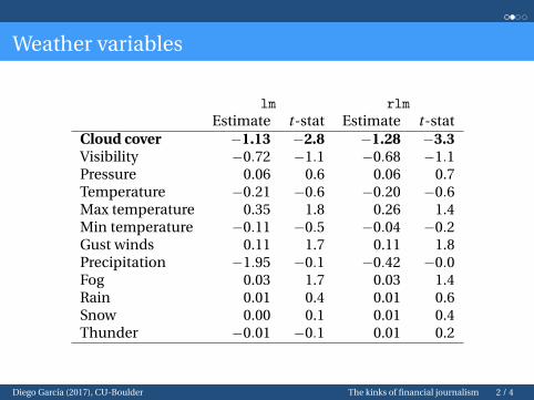
Estimate t-stat Estimate t-statCloud cover −1.13 −2.8 −1.28 −3.3Visibility −0.72 −1.1 −0.68 −1.1Pressure 0.06 0.6 0.06 0.7Temperature −0.21 −0.6 −0.20 −0.6Max temperature 0.35 1.8 0.26 1.4Min temperature −0.11 −0.5 −0.04 −0.2Gust winds 0.11 1.7 0.11 1.8Precipitation −1.95 −0.1 −0.42 −0.0Fog 0.03 1.7 0.03 1.4Rain 0.01 0.4 0.01 0.6Snow 0.00 0.1 0.01 0.4Thunder −0.01 −0.1 0.01 0.2
Diego Garcı́a (2017), CU-Boulder The kinks of financial journalism 2 / 4
Calendar effects
lm rlm
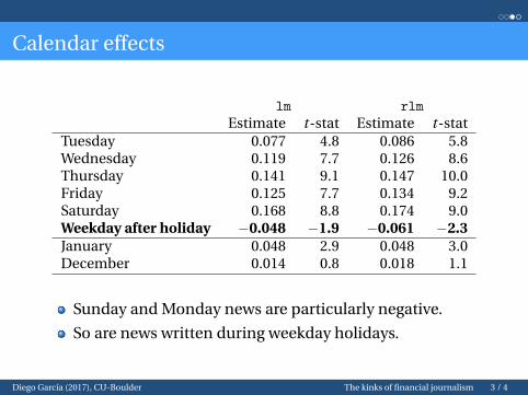
Estimate t-stat Estimate t-statTuesday 0.077 4.8 0.086 5.8Wednesday 0.119 7.7 0.126 8.6Thursday 0.141 9.1 0.147 10.0Friday 0.125 7.7 0.134 9.2Saturday 0.168 8.8 0.174 9.0Weekday after holiday −0.048 −1.9 −0.061 −2.3January 0.048 2.9 0.048 3.0December 0.014 0.8 0.018 1.1
Sunday and Monday news are particularly negative.
So are news written during weekday holidays.
Diego Garcı́a (2017), CU-Boulder The kinks of financial journalism 3 / 4
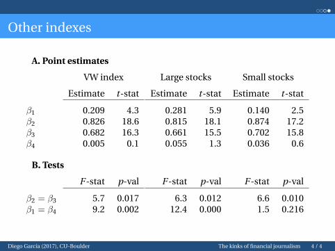
Other indexes
A. Point estimates
VW index Large stocks Small stocks
Estimate t-stat Estimate t-stat Estimate t-stat
β1 0.209 4.3 0.281 5.9 0.140 2.5β2 0.826 18.6 0.815 18.1 0.874 17.2β3 0.682 16.3 0.661 15.5 0.702 15.8β4 0.005 0.1 0.055 1.3 0.036 0.6
B. Tests
F -stat p-val F -stat p-val F -stat p-val
β2 = β3 5.7 0.017 6.3 0.012 6.6 0.010β1 = β4 9.2 0.002 12.4 0.000 1.5 0.216
Diego Garcı́a (2017), CU-Boulder The kinks of financial journalism 4 / 4