Embed Size (px)
Citation preview
4
For help in preparation of this article, thanKehrer, NLfB-KTB, Hannover, Germany; HJochen Kück, Manfred Neuber, Thomas RöSowa and Klaus Sturmeit, Windischeschenmany; Karl Bohn and Ignaz de Grefte, SchWireline & Testing, Windischeschenbach,Howard, Schlumberger Wireline & TestingTexas, USA; Jörn Lauterjung, GFZ InstituteGermany; N. Riquier and Alain Poizat, SchWireline & Testing, Abbeville, France.In this article CSU (wellsite surface instrumFMI (Fullbore Formation MicroImager), FoMicroScanner, GLT (Geochemical LoggingLitho-Density, NGS (Natural Gamma Ray and Sidewall CoreDriller are marks of SchVAX is a mark of Digital Equipment Corpo
The drill bit has stopped turning and the KTB project is winding down.
complete. How and why was it drilled?
ieved so far?
Kurt BramJohann DraxlerGottfried HirschmannGustav ZothNLfB-KTBHannover, Germany
Stephane HironClamart, France
Miel KührWindischeschenbach, Germany
The KTB Borehole—Germany’s Superdeep Telescope into the Earth’s Crust
essnd total ofin- asck
idengicsndngns
specifically for scientific research only withinthe last thirty years.
The internationally funded Ocean DrillingProgram (ODP) was started as part of aworldwide effort to research the hard outerlayer of the Earth’s crust called the litho-sphere.1 Results from this project have beendramatic, providing real evidence of conti-nental drift and plate tectonics. The litho-sphere is made up of six major and severalminor rigid moving plates. New oceaniccrust is formed and spreads out at mid-oceanridges and is consumed at active plate mar-gins—subduction zones—where it sinks
annover
SCIENTIFIC DRILLING
ks to Peterorst Gatto,ckel, Michaelbach, Ger-lumberger Germany; Pete, Houston,, Potsdam,lumberger
entation), rmation Tool),
Spectrometry)lumberger.ration.
Germany’s superdeep borehole is
And what have the scientists ach
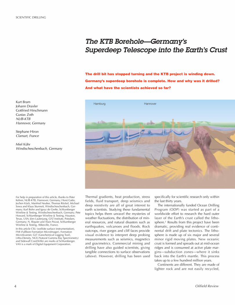
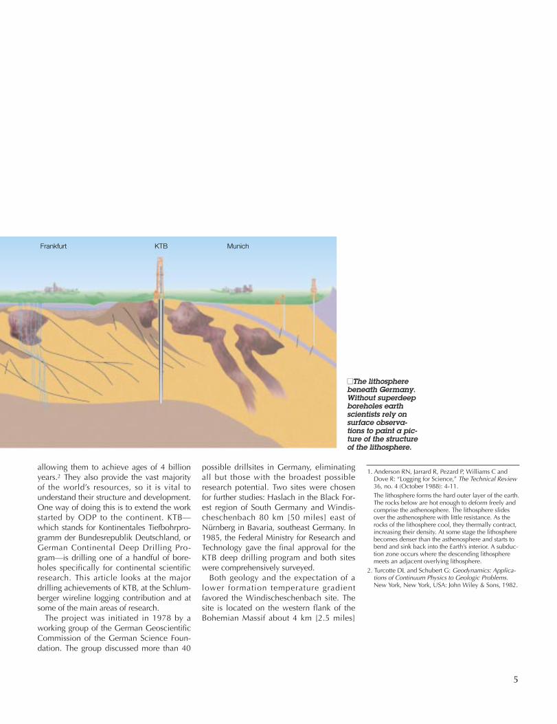
Thermal gradients, heat production, strfields, fluid transport, deep seismics adeep resistivity are all of great interestearth scientists. Studying these fundamentopics helps them unravel the mysteriesweather fluctuations, the distribution of meral resources, and natural disasters suchearthquakes, volcanoes and floods. Rooutcrops, river gorges and cliff faces provvisual evidence to interpret deep probimeasurements such as seismics, magnetand gravimetrics. Commercial mining adrilling have also guided scientists, givitangible connections to surface observatio
Hamburg H
Oilfield Review
(above). However, drilling has been used back into the Earth’s mantle. This processtakes up to a few hundred million years.
Continents are different. They are made oflighter rock and are not easily recycled,
5
■■The lithospherebeneath Germany.Without superdeepboreholes earthscientists rely onsurface observa-tions to paint a pic-ture of the structureof the lithosphere.
1. Anderson RN, Jarrard R, Pezard P, Williams C andDove R: “Logging for Science,” The Technical Review36, no. 4 (October 1988): 4-11.The lithosphere forms the hard outer layer of the earth.The rocks below are hot enough to deform freely andcomprise the asthenosphere. The lithosphere slidesover the asthenosphere with little resistance. As therocks of the lithosphere cool, they thermally contract,increasing their density. At some stage the lithospherebecomes denser than the asthenosphere and starts tobend and sink back into the Earth’s interior. A subduc-tion zone occurs where the descending lithospheremeets an adjacent overlying lithosphere.
2. Turcotte DL and Schubert G: Geodynamics: Applica-tions of Continuum Physics to Geologic Problems.New York, New York, USA: John Wiley & Sons, 1982.
allowing them to achieve ages of 4 billionyears.2 They also provide the vast majorityof the world’s resources, so it is vital tounderstand their structure and development.One way of doing this is to extend the workstarted by ODP to the continent. KTB—which stands for Kontinentales Tiefbohrpro-gramm der Bundesrepublik Deutschland, orGerman Continental Deep Drilling Pro-gram—is drilling one of a handful of bore-holes specifically for continental scientificresearch. This article looks at the majordrilling achievements of KTB, at the Schlum-berger wireline logging contribution and atsome of the main areas of research.
The project was initiated in 1978 by aworking group of the German GeoscientificCommission of the German Science Foun-dation. The group discussed more than 40
possible drillsites in Germany, eliminatingall but those with the broadest possibleresearch potential. Two sites were chosenfor further studies: Haslach in the Black For-est region of South Germany and Windis-cheschenbach 80 km [50 miles] east ofNürnberg in Bavaria, southeast Germany. In1985, the Federal Ministry for Research andTechnology gave the final approval for theKTB deep drilling program and both siteswere comprehensively surveyed.
Both geology and the expectation of alower formation temperature gradientfavored the Windischeschenbach site. Thesite is located on the western flank of theBohemian Massif about 4 km [2.5 miles]
Frankfurt KTB Munich
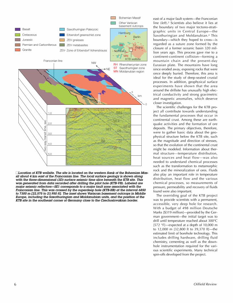
east of a major fault system—the Franconianline (left).3 Scientists also believe it lies atthe boundary of two major tectono-strati-graphic units in Central Europe—theSaxothuringian and Moldanubian.4 Thisboundary—which they hoped to cross—isregarded as a suture zone formed by theclosure of a former oceanic basin 320 mil-lion years ago. This process gave rise to acontinent-continent collision—forming amountain chain and the present-dayEurasian plate. The mountains have longsince eroded away, exposing rocks that wereonce deeply buried. Therefore, this area isideal for the study of deep-seated crustalprocesses. In addition, geophysical surfaceexperiments have shown that the areaaround the drillsite has unusually high elec-trical conductivity and strong gravimetricand magnetic anomalies, which deservecloser investigation.
The scientific challenges for the KTB pro-ject all contribute towards understandingthe fundamental processes that occur incontinental crust. Among these are earth-quake activities and the formation of oredeposits. The primary objectives, therefore,were to gather basic data about the geo-physical structure below the KTB site, suchas the magnitude and direction of stresses,so that the evolution of the continental crustmight be modeled. Information about ther-mal structure—temperature distribution,heat sources and heat flow—was alsoneeded to understand chemical processessuch as the transformation to metamorphicrock and the mineralization of ores. Fluidsalso play an important role in temperaturedistribution, heat flow and the variouschemical processes, so measurements ofpressure, permeability and recovery of fluidsfound were also important.
The overriding goal of the KTB projectwas to provide scientists with a permanent,accessible, very deep hole for research.With a budget of 498 million DeutscheMarks [$319 million]—provided by the Ger-man government—the initial target was todrill until temperature reached about 300°C[572 °F]—expected at a depth of 10,000 mto 12,000 m [32,800 ft to 39,370 ft]—theestimated limit of borehole technology. Thisincludes drilling hardware, drilling fluidchemistry, cementing as well as the down-hole instrumentation required for the vari-ous scientific experiments. Many technicalspin-offs developed from the project.
6 Oilfield Review
■■Location of KTB wellsite. The site is located on the western flank of the Bohemian Mas-sif about 4 km east of the Franconian line. The local surface geology is shown alongwith the three-dimensional (3D) surface seismic time slice beneath the KTB site. Thiswas generated from data recorded after drilling the pilot hole (KTB-VB). Labeled aremajor seismic reflectors—SE1 corresponds to a major fault zone associated with theFranconian line. This was crossed by the superdeep hole (KTB-HB) at the interval 6850to 7300 m [22,575 to 23,950 ft]. The inset shows Variscan basement outcrops in MiddleEurope, including the Saxothuringian and Moldanubian units, and the position of theKTB site in the southeast corner of Germany close to the Czechoslovakian border.
Basalt
NW
NE
0
5
km
1.0
2.0
3.0
4.0
5.0
Two-
way
tran
sit t
ime,
sec
Franconian line
Other Variscanbasement outcrops
Rhenohercynian zoneSaxothuringian zoneMoldanubian region
RH ST
MNKTB wellsite
RHSTMN
ZEV- Zone of Erbendorf Vohenstrauss
HamburgBerlin
NürnbergPraha
Saxothuringian Paleozoic
Cretaceous
Jurassic
Permian and Carboniferous
Granite
Erbendorf greenschist zone
ZEV gneisses
ZEV metabasites
Bohemian Massif
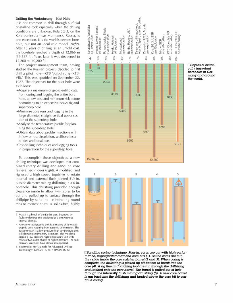
Drilling the Vorbohrung—Pilot HoleIt is not common to drill through surficialcrystalline rock especially when the drillingconditions are unknown. Kola SG 3, on theKola peninsula near Murmansk, Russia, isone exception. It is the world’s deepest bore-hole, but not an ideal role model (right).After 15 years of drilling, at an untold cost,the borehole reached a depth of 12,066 m[39,587 ft]. Years later it was deepened to12,260 m [40,200 ft].
The project management team, havingstudied the Russian project, decided to firstdrill a pilot hole—KTB Vorbohrung (KTB-VB).5 This was spudded on September 22,1987. The objectives for the pilot hole wereas follows:•Acquire a maximum of geoscientific data,
from coring and logging the entire bore-hole, at low cost and minimum risk beforecommitting to an expensive heavy rig andsuperdeep hole.
•Minimize core runs and logging in thelarge-diameter, straight vertical upper sec-tion of the superdeep hole.
•Analyze the temperature profile for plan-ning the superdeep hole.
•Obtain data about problem sections withinflow or lost circulation, wellbore insta-bilities and breakouts.
•Test drilling techniques and logging toolsin preparation for the superdeep hole.
To accomplish these objectives, a newdrilling technique was developed that com-bined rotary drilling and sandline coreretrieval techniques (right). A modified landrig used a high-speed topdrive to rotateinternal and external flush-jointed 51/2-in.outside diameter mining drillstring in a 6-in.borehole. This drillstring provided enoughclearance inside to allow 4-in. cores to becut and pulled up to surface through thedrillpipe by sandline—eliminating roundtrips to recover cores. A solids-free, highly
7January 1995
■■Depths of histori-cally importantboreholes in Ger-many and aroundthe world.
■■Sandline coring technique. Four-in. cores are cut with high-perfor-mance, impregnated diamond core bits (1). As the cores are cut,they slide inside the core catcher barrel (2 and 3). When coring iscomplete, the drillstring is picked up off bottom to break free thecore (4). A rig line and latching tool are run through the drillstringand latched onto the core barrel. The barrel is pulled out-of-holethrough the internally flush mining drillstring (5). A new core barrelis run back into the drillstring and landed above the core bit to con-tinue coring.
3. Massif is a block of the Earth’s crust bounded by faults or flexures and displaced as a unit without internal change.
4. A tectono-stratigraphic unit is a mixture of lithostrati-graphic units resulting from tectonic deformation. TheSaxothurigian is a low pressure-high temperature unitstill showing sedimentary structures. The Moldanu-bian is a low pressure-high temperature unit withrelics of two older phases of higher pressure. The sedi-mentary structures have almost disappeared.
5. Rischmüller H: “Example for Advanced Drilling Technology,” Oil Gas 16, no. 4 (1990): 16-20.
Neu
salz
wer
k, W
estfa
liasa
lt ex
plor
atio
n
69535
2003
3818
5966
9583
3930
8553
8008
4000
12,260
9101
1847
Wie
tze,
Low
er S
axon
yoi
l exp
lora
tion
1858
Por
usch
owitz
, Sile
sia
coal
exp
lora
tion
1893
Hei
de, H
olst
ein
oil e
xplo
ratio
n19
38
Mun
ster
land
gas
expl
orat
ion
1962
Ber
tha
Rog
ers,
US
Aga
s ex
plor
atio
n19
74
Dee
p se
a dr
illing
pro
ject
,A
tlant
ic, S
pain
, sci
entif
ic d
rillin
g19
76
Zist
ersd
orf U
T-2,
Aus
tria
gas
expl
orat
ion
1983
Kol
a S
G 3
, US
SR
gas
Exp
lora
tion
1985
Miro
w, G
DR
scie
ntifi
c dr
illing
1985
KTB
Obe
rpfa
lz V
Bsc
ient
ific
drilli
ng19
89
KTB
Obe
rpfa
lz H
Bsc
ient
ific
drilli
ng19
94
Depth, m
1 2 3 4 5
✓
✓
✓
✓
✓
✓
✓
✓
✓
✓
✓
✓
✓
✓
✓
✓
✓
✓
✓
✓
✓
✓
✓
✓
✓
KTB Logging ToolsAuxiliary Measurement Sonde1
Borehole Geometry Tool1
Colliding Detonation Drill Collar Cutter2
Fluid Sampler
Formation MicroScanner*1
Gamma Ray1
Self Potential
Single Shot
Temperature Tool
6-Arm Caliper
* Mark of Schlumberger1 Bought from or developed by Schlumberger for KTB2 Developed by SwETech (Bofors) for KTB
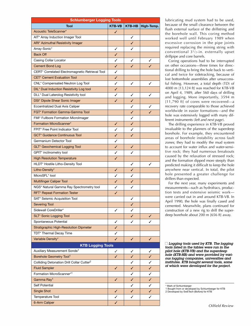
lubricating mud system had to be used,because of the small clearance between theflush external surface of the drillstring andthe borehole wall. This coring methodworked well until February 1989 whenexcessive corrosion in the pipe jointsrequired replacing the mining string withconventional 31/2-in. externally upsetdrillpipe and core barrels.
Coring operations had to be interruptedon other occasions—three times for direc-tional drilling to bring the hole back to verti-cal and twice for sidetracking, because oflost bottomhole assemblies after unsuccess-ful fishing. However, a total depth (TD) of4000 m [13,124 ft] was reached for KTB-VBon April 4, 1989, after 560 days of drillingand logging. More importantly, 3594 m[11,790 ft] of cores were recovered—arecovery rate comparable to those achievedworldwide in easier formations—and thehole was extensively logged with many dif-ferent instruments (left and next page).
The drilling experience in KTB-VB provedinvaluable to the planners of the superdeepborehole. For example, they encounteredareas of borehole instability across faultzones; they had to modify the mud systemto account for water influx and water-sensi-tive rock; they had numerous breakoutscaused by the relaxation of stressed rock;and the formation dipped more steeply thanpredicted making it difficult to keep the holeanywhere near vertical. In total, the pilothole presented a greater challenge fordrillers than expected.
For the next year, many experiments andmeasurements—such as hydrofracs, produc-tion tests and extensive seismic work—were carried out in and around KTB-VB. InApril 1990, the hole was finally cased andcemented. Meanwhile, plans continued forconstruction of a new rig to drill the super-deep borehole about 200 m [656 ft] away.
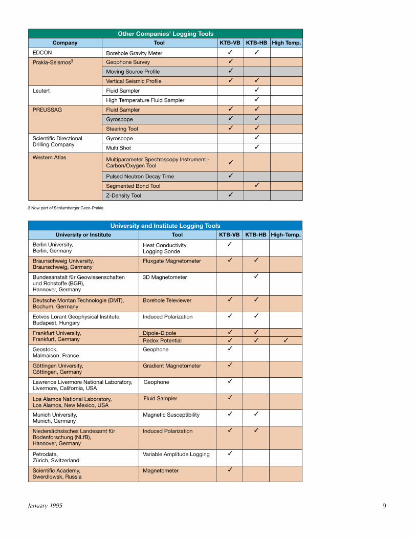
■■ Logging tools used by KTB. The loggingtools listed in the tables were run in thepilot hole (KTB-VB) and the superdeephole (KTB-HB) and were provided by vari-ous logging companies, universities andinstitutes. KTB bought several tools, someof which were developed for the project.
Oilfield Review
Schlumberger Logging Tools
Tool
Acoustic TeleScanner* ✓
✓
✓
✓
✓
✓
✓
✓
✓
✓
✓
✓
✓
✓
✓
✓
✓
✓
✓
✓
✓
✓
✓
✓
✓
✓
✓
✓
✓
✓
✓
✓
✓
✓
✓
✓
✓
✓
✓
✓
✓
✓
✓
✓
✓
✓
✓
✓
✓
✓
✓
✓
✓
✓
✓
✓
✓
✓
✓
✓
✓
✓
✓
✓
✓
AIT* Array Induction Imager Tool
ARI* Azimuthal Resistivity Imager
Array-Sonic*
Back Off
Casing Collar Locator
Cement Bond Log
CERT* Correlated Electromagnetic Retrieval Tool
CET* Cement Evaluation Tool
CNL* Compensated Neutron Log Tool
DIL* Dual Induction Resistivity Log tool
DLL* Dual Laterolog Resistivity tool
DSI* Dipole Shear Sonic Imager
Eccentralized Dual Axis Caliper
FGT* Formation Gamma-Gamma Tool
FMI* Fullbore Formation MicroImager
Formation MicroScanner*
FPIT* Free Point Indicator Tool
GCT* Guidance Continuous Tool
Germanium Detector Tool
GLT* Geochemical Logging Tool
GPIT* inclinometry tool
High Resolution Temperature
HLDT* Hostile Litho-Density Tool
Litho-Density*
MicroSFL* tool
Multifinger Caliper Tool
NGS* Natural Gamma Ray Spectrometry tool
RFT* Repeat Formation Tester
SAT* Seismic Acquisition Tool
Severing Tool
Sidewall CoreDriller*
SLT* Sonic Logging Tool
Spontaneous Potential
Stratigraphic High-Resolution Dipmeter
TDT* Thermal Decay Time
Variable Density*
KTB-VB KTB-HB High-Temp.
9January 1995
University and Institute Logging ToolsUniversity or Institute
Berlin University, Berlin, Germany
Braunschweig University, Braunschweig, Germany
Bundesanstalt für Geowissenschaften und Rohstoffe (BGR), Hannover, Germany
Deutsche Montan Technologie (DMT), Bochum, Germany
Eötvös Lorant Geophysical Institute, Budapest, Hungary
Frankfurt University, Frankfurt, Germany
Geostock, Malmaison, France
Göttingen University, Göttingen, Germany
Los Alamos National Laboratory, Los Alamos, New Mexico, USA
Munich University, Munich, Germany
Niedersächsisches Landesamt für Bodenforschung (NLfB), Hannover, Germany
Petrodata, Zürich, Switzerland
Scientific Academy, Swerdlowsk, Russia
Heat Conductivity Logging Sonde
✓
✓
✓
✓
✓
✓
✓ ✓
✓
✓
✓
✓
✓
✓
✓
✓
✓
✓
✓
✓
✓
✓
✓
Fluxgate Magnetometer
3D Magnetometer
Borehole Televiewer
Induced Polarization
Dipole-DipoleRedox Potential
Geophone
Gradient Magnetometer
Geophone
Fluid Sampler
Magnetic Susceptibility
Induced Polarization
Variable Amplitude Logging
Magnetometer
Tool KTB-VB KTB-HB High-Temp.
Lawrence Livermore National Laboratory, Livermore, California, USA
3 Now part of Schlumberger Geco-Prakla
Other Companies’ Logging ToolsCompany
EDCON
Prakla-Seismos3
Leutert
PREUSSAG
Scientific Directional Drilling Company
Western Atlas
Borehole Gravity Meter ✓ ✓
✓
✓
✓
✓
✓
✓
✓
✓
✓
✓
✓
✓
✓
✓
✓
✓
✓
✓
Geophone Survey
Moving Source Profile
Vertical Seismic Profile
Fluid Sampler
High Temperature Fluid Sampler
Fluid Sampler
Gyroscope
Steering Tool
Gyroscope
Multi Shot
Multiparameter Spectroscopy Instrument - Carbon/Oxygen Tool
Pulsed Neutron Decay Time
Segmented Bond Tool
Z-Density Tool
Tool KTB-VB KTB-HB High Temp.
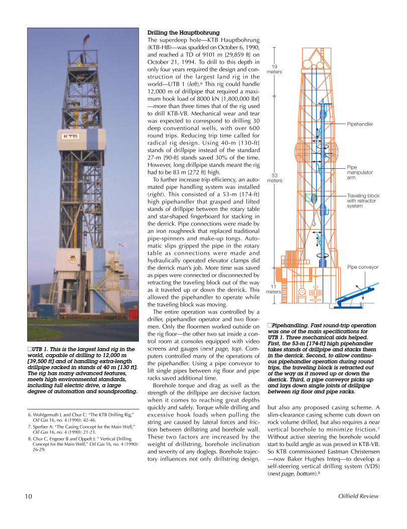
Drilling the HauptbohrungThe superdeep hole—KTB Hauptbohrung(KTB-HB)—was spudded on October 6, 1990,and reached a TD of 9101 m [29,859 ft] onOctober 21, 1994. To drill to this depth inonly four years required the design and con-struction of the largest land rig in theworld—UTB 1 (left).6 This rig could handle12,000 m of drillpipe that required a maxi-mum hook load of 8000 kN [1,800,000 lbf]—more than three times that of the rig usedto drill KTB-VB. Mechanical wear and tearwas expected to correspond to drilling 30deep conventional wells, with over 600round trips. Reducing trip time called forradical rig design. Using 40-m [130-ft]stands of drillpipe instead of the standard27-m [90-ft] stands saved 30% of the time.However, long drillpipe stands meant the righad to be 83 m [272 ft] high.
To further increase trip efficiency, an auto-mated pipe handling system was installed(right ). This consisted of a 53-m [174-ft]high pipehandler that grasped and liftedstands of drillpipe between the rotary tableand star-shaped fingerboard for stacking inthe derrick. Pipe connections were made byan iron roughneck that replaced traditionalpipe-spinners and make-up tongs. Auto-matic slips gripped the pipe in the rotarytable as connections were made andhydraulically operated elevator clamps didthe derrick man’s job. More time was savedas pipes were connected or disconnected byretracting the traveling block out of the wayas it traveled up or down the derrick. Thisallowed the pipehandler to operate whilethe traveling block was moving.
The entire operation was controlled by adriller, pipehandler operator and two floor-men. Only the floormen worked outside onthe rig floor—the other two sat inside a con-trol room at consoles equipped with videoscreens and gauges (next page, top). Com-puters controlled many of the operations ofthe pipehandler. Using a pipe conveyor tolift single pipes between rig floor and piperacks saved additional time.
Borehole torque and drag as well as thestrength of the drillpipe are decisive factorswhen it comes to reaching great depthsquickly and safely. Torque while drilling andexcessive hook loads when pulling thestring are caused by lateral forces and fric-tion between drillstring and borehole wall.These two factors are increased by theweight of drillstring, borehole inclinationand severity of any doglegs. Borehole trajec-tory influences not only drillstring design,
but also any proposed casing scheme. Aslim-clearance casing scheme cuts down onrock volume drilled, but also requires a nearvertical borehole to minimize friction.7
Without active steering the borehole wouldstart to build angle as was proved in KTB-VB.So KTB commissioned Eastman Christensen—now Baker Hughes Inteq—to develop aself-steering vertical drilling system (VDS)(next page, bottom).8
10 Oilfield Review
■■Pipehandling. Fast round-trip operationwas one of the main specifications for UTB 1. Three mechanical aids helped.First, the 53-m [174-ft] high pipehandlertakes stands of drillpipe and stacks themin the derrick. Second, to allow continu-ous pipehandler operation during roundtrips, the traveling block is retracted outof the way as it moved up or down thederrick. Third, a pipe conveyor picks upand lays down single joints of drillpipebetween rig floor and pipe racks.
■■UTB 1. This is the largest land rig in theworld, capable of drilling to 12,000 m[39,500 ft] and of handling extra-lengthdrillpipe racked in stands of 40 m [130 ft].The rig has many advanced features,meets high environmental standards,including full electric drive, a largedegree of automation and soundproofing.
6. Wohlgemuth L and Chur C: “The KTB Drilling Rig,”Oil Gas 16, no. 4 (1990): 42-46.
7. Sperber A: “The Casing Concept for the Main Well,”Oil Gas 16, no. 4 (1990): 21-23.
8. Chur C, Engeser B and Oppelt J: “ Vertical DrillingConcept for the Main Well,” Oil Gas 16, no. 4 (1990):26-29.
Pipehandler
Pipemanipulatorarm
Traveling blockwith retractorsystem
Pipe conveyor
53meters
19meters
11meters
11January 1995
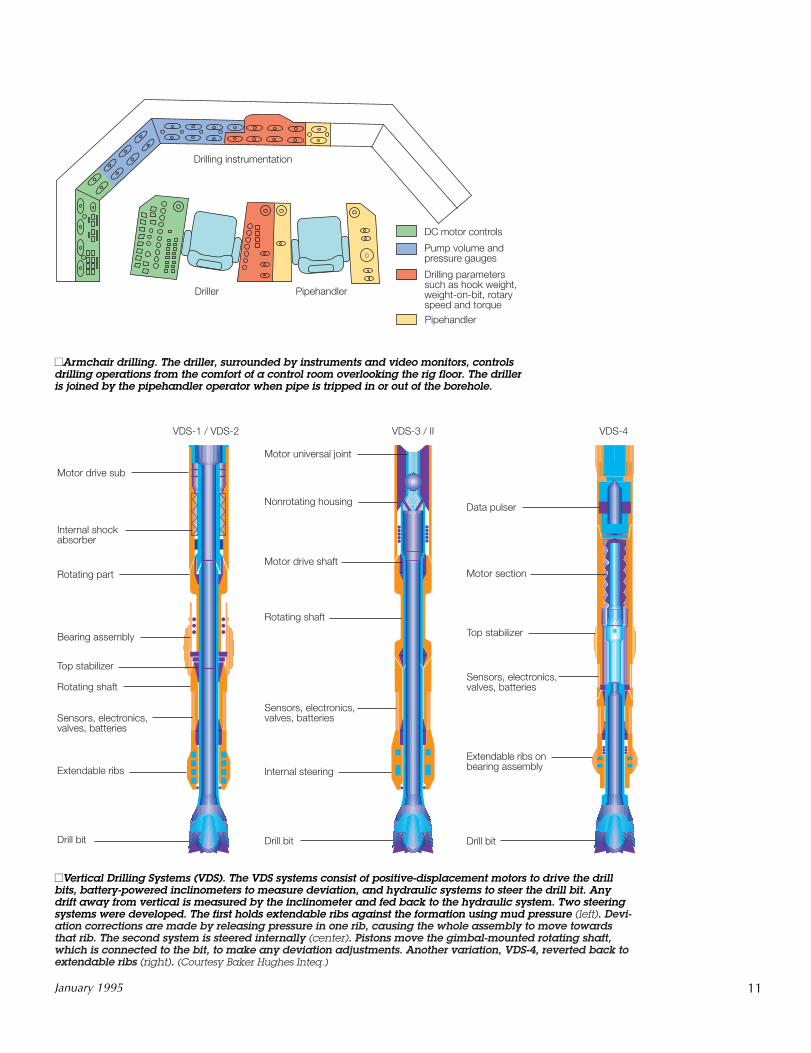
■■Armchair drilling. The driller, surrounded by instruments and video monitors, controlsdrilling operations from the comfort of a control room overlooking the rig floor. The drilleris joined by the pipehandler operator when pipe is tripped in or out of the borehole.
■■Vertical Drilling Systems (VDS). The VDS systems consist of positive-displacement motors to drive the drillbits, battery-powered inclinometers to measure deviation, and hydraulic systems to steer the drill bit. Anydrift away from vertical is measured by the inclinometer and fed back to the hydraulic system. Two steeringsystems were developed. The first holds extendable ribs against the formation using mud pressure (left). Devi-ation corrections are made by releasing pressure in one rib, causing the whole assembly to move towardsthat rib. The second system is steered internally (center). Pistons move the gimbal-mounted rotating shaft,which is connected to the bit, to make any deviation adjustments. Another variation, VDS-4, reverted back toextendable ribs (right). (Courtesy Baker Hughes Inteq.)
Drilling instrumentation
Driller Pipehandler
DC motor controls
Pump volume andpressure gauges
Drilling parameterssuch as hook weight,weight-on-bit, rotaryspeed and torquePipehandler
Motor drive sub
Internal shockabsorber
Rotating part
Bearing assembly
Top stabilizer
Rotating shaft
Sensors, electronics,valves, batteries
Extendable ribs
Drill bit
VDS-1 / VDS-2
Motor universal joint
Rotating shaft
Motor drive shaft
Sensors, electronics,valves, batteries
Internal steering
Drill bit
Nonrotating housing
VDS-3 / II
Data pulser
Motor section
Top stabilizer
Sensors, electronics,valves, batteries
Extendable ribs onbearing assembly
Drill bit
VDS-4
12
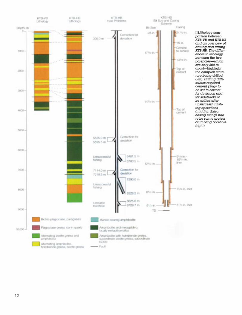
■■Lithology com-parison betweenKTB-VB and KTB-HBand an overview ofdrilling and casingKTB-HB. The differ-ences in lithologybetween the twoboreholes—whichare only 200 mapart—highlightthe complex struc-ture being drilled(left). Drilling diffi-culties requiredcement plugs to be set to correct for deviation andfor sidetracks to be drilled afterunsuccessful fish-ing operations(middle). Extra casing strings hadto be run to protectcrumbling borehole(right).
The VDS system consisted of a positive-displacement motor to drive the drill bit, abattery-powered inclinometer to measuredeviation and a hydraulic system to adjustthe angle of the drill bit to correct for devia-tion. Two hydraulic systems were used: thefirst system operated external stabilizer ribsthat pushed against the borehole wall mov-ing the whole VDS assembly back to thevertical; the second system used internalrams to move the shaft driving the drill bitback to vertical. As long as battery powerwas maintained to the inclinometer, bothsystems operated automatically. Inclination,and other parameters such as temperature,voltage and systems pressure, were trans-mitted to surface by a mud pulser to moni-tor progress.
The first 292 m [958 ft] of KTB-HB weredrilled with a 171/2-in. bit and opened up to28 in. before setting the 241/2-in. casing(previous page). To meet the requirementsof a vertical hole, a 2.5° correction to devia-tion was made as the hole was widened.The next section was drilled with a 171/2-in.VDS system to 3000 m [9840 ft] and com-pleted at the end of May 1991. Teethingproblems with prototype VDS systemsmeant using packed-hole assemblies (PHAs)during maintenance and repair. Even so,average deviation for this section was lessthan 0.5°.
The same strategy was used for the 143/4-in.hole—alternating between the improvingVDS systems and PHAs. A high deviationbuildup from 5519 to 5596 m [18,107 to18,360 ft] during one PHA run led to theborehole being pulled back and a correc-tion made for deviation. The hole contin-ued on course to 6013 m [19,728 ft] where133/8-in. casing was set in April 1992—hor-izontal displacement at this stage was lessthan 10 m [33 ft].
Drilling continued with VDS systems andPHAs and 121/4-in. bits. Within this section45.7 m [150 ft] were cored, including 20.7 m[68 ft] with a newly developed, large-diam-eter coring system that gave 91/4-in. diame-ter cores. However, in July 1992 at 6760 m[22,179 ft], the bit became stuck. Eventually,after an unsuccessful fishing operation, thehole had to be plugged back to 6461 m[21,198 ft] and sidetracked. In March 1993,over an interval of 6850 to 7300 m [22,474to 23,950 ft], a major fault system wascrossed. The VDS system could not controldeviation over this interval and another cor-rection had to be made. This system wasthought to be an extension of the main faultthat lies along the boundary between sedi-
ments to the west and metamorphic rocks tothe east—the Franconian line. Along thisfault system a displacement of more than3000 m occurred, showing a repetition ofdrilled rock sequences. This signaled thestart of the most difficult drilling yet andadditional funds had to be provided by theGerman government to complete the project—bringing the total cost to DM 528 million[$338 million].
At 7490 m [24,573 ft], when the horizon-tal displacement was only 12 m [39 ft], theVDS system was abandoned, as boreholetemperatures became too high for the elec-tronics. The hole then started to deviatenorth (below). Within the main fault systemthe borehole became unstable and morebreakouts occurred. While tripping out-of-hole from 8328 m [27,323 ft], the drillpipebecame stuck at 7523 m [24,682 ft]. Jarringeventually broke the downhole motor hous-ing allowing the pipe to be pulled out butleaving behind a complicated fish. Severalattempts to retrieve the fish failed and the
hole was finally plugged back to the verticalsection—at 7390 m [24,245 ft]—and side-tracked. Drilling again proved difficult andso a 95/8-in. liner was set at 7785 m [25,541ft] in December 1993 to protect this hard-won section of hole.
Difficult drilling continued with a 81/2-in.bit down to 8730 m [28,642 ft]. Boreholeinstability prevented further progress and a75/8-in. liner was set in May 1994. To bypassthe unstable section, a sidetrack was made at8625 m [28,297 ft] through a precut windowin the liner. Funds to continue drilling werenow running low and a decision was madeto stop 476 m [1561 ft] later on October 12,1994. More than four years after spudding,the hole had reached 9101 m with a final bitsize of 61/2 in. However, the borehole hadnot finished with the drillers yet. Attempts tolower logging tools into the open hole failed.The last section had to be re-drilled and a51/2-in. liner set, leaving only 70 m [230 ft]of open hole for the wireline loggers andother scientific experiments.
13January 1995
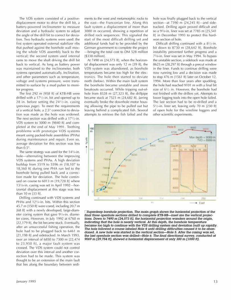
■■Superdeep borehole projection. The main graph shows the horizontal projection of thefinal three openhole sections drilled to complete KTB-HB—inset are the vertical projec-tions. Down to 7490 m [24,573 ft], the horizontal projection wanders around the origin,indicating that the hole is nearly vertical. At this depth, the borehole temperaturebecame too high to continue with the VDS drilling system and deviation built up rapidly.The hole followed a course labeled Hole 4 until drilling difficulties caused it to be aban-doned. A new hole was started in the vertical section—Hole 5. After the casing was set,the last openhole section was drilled—Hole 6. The final directional survey, conducted at9069 m [29,754 ft], showed a horizontal displacement of only 300 m [1000 ft].
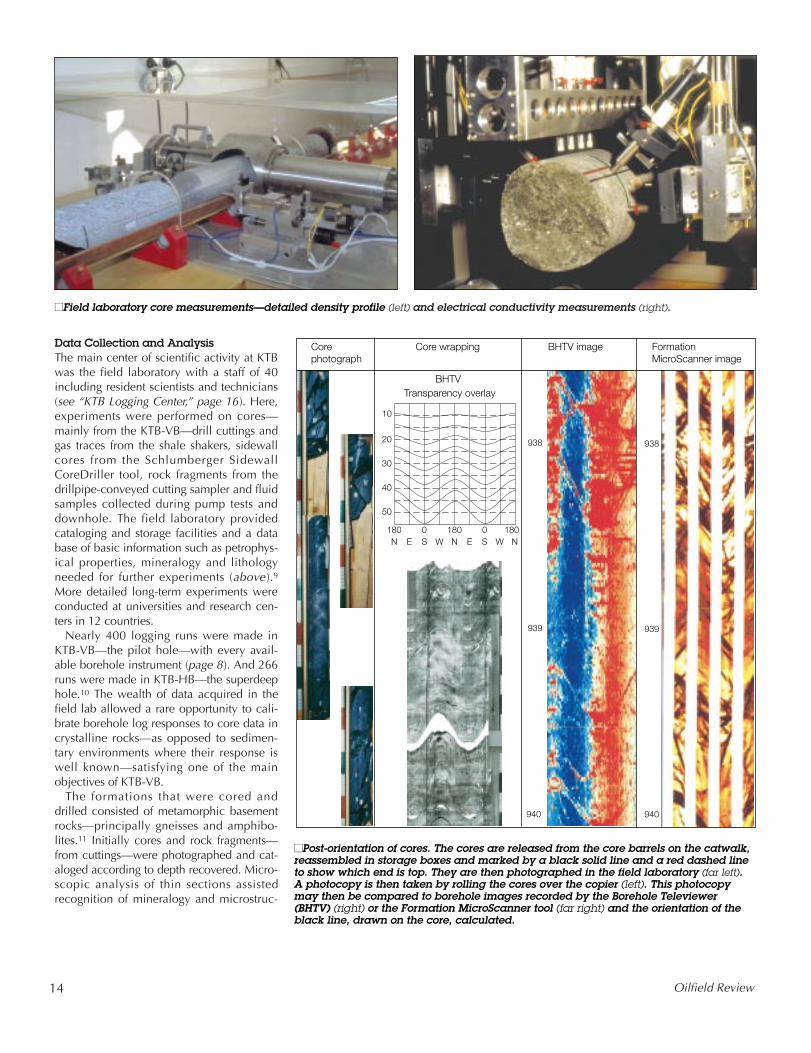
Data Collection and AnalysisThe main center of scientific activity at KTBwas the field laboratory with a staff of 40including resident scientists and technicians(see “KTB Logging Center,” page 16). Here,experiments were performed on cores—mainly from the KTB-VB—drill cuttings andgas traces from the shale shakers, sidewallcores from the Schlumberger SidewallCoreDriller tool, rock fragments from thedrillpipe-conveyed cutting sampler and fluidsamples collected during pump tests anddownhole. The field laboratory providedcataloging and storage facilities and a database of basic information such as petrophys-ical properties, mineralogy and lithologyneeded for further experiments (above).9More detailed long-term experiments wereconducted at universities and research cen-ters in 12 countries.
Nearly 400 logging runs were made inKTB-VB—the pilot hole—with every avail-able borehole instrument (page 8). And 266runs were made in KTB-HB—the superdeephole.10 The wealth of data acquired in thefield lab allowed a rare opportunity to cali-brate borehole log responses to core data incrystalline rocks—as opposed to sedimen-tary environments where their response iswell known—satisfying one of the mainobjectives of KTB-VB.
The formations that were cored anddrilled consisted of metamorphic basementrocks—principally gneisses and amphibo-lites.11 Initially cores and rock fragments—from cuttings—were photographed and cat-aloged according to depth recovered. Micro-scopic analysis of thin sections assistedrecognition of mineralogy and microstruc-
14 Oilfield Review
■■Field laboratory core measurements—detailed density profile (left) and electrical conductivity measurements (right).
■■Post-orientation of cores. The cores are released from the core barrels on the catwalk,reassembled in storage boxes and marked by a black solid line and a red dashed lineto show which end is top. They are then photographed in the field laboratory (far left). A photocopy is then taken by rolling the cores over the copier (left). This photocopymay then be compared to borehole images recorded by the Borehole Televiewer(BHTV) (right) or the Formation MicroScanner tool (far right) and the orientation of theblack line, drawn on the core, calculated.
BHTVTransparency overlay
938
939
940
938
50
180N E S W N NE S W
0 180 1800
10
20
30
40
939
940
Corephotograph
Core wrapping BHTV image FormationMicroScanner image
ture and assignment of rock type.12 By map-ping the macroscopic structure and orientingit with borehole logs such as the FMI Full-bore Formation MicroImager image or Bore-hole Televiewer (BHTV) image, a structuralpicture of the borehole was gradually builtup (previous page, bottom).
Petrophysical parameters, such as thermalconductivity, density, electrical conductivity,acoustic impedance, natural radioactivity,natural remanent magnetism and magneticsusceptibility were also routinely measured.In addition to determining the strength ofrock samples, scientists made highly sensi-tive measurements of expansion of the coresas they relaxed to atmospheric pressure.
Geochemists at the field laboratory per-formed detailed core analysis using X-rayfluorescence for rock chemical compositionand X-ray diffraction for mineralogy.13 Thisanalysis allowed a reliable reconstruction ofthe lithology.
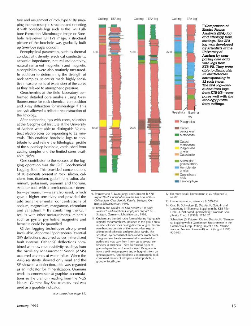
After comparing logs with cores, scientistsat the Geophysical Institute at the Universityof Aachen were able to distinguish 32 dis-tinct electrofacies corresponding to 32 min-erals. This enabled borehole logs to con-tribute to and refine the lithological profileof the superdeep borehole, established fromcutting samples and the limited cores avail-able (right).
One contributor to the success of the log-ging operation was the GLT GeochemicalLogging Tool. This provided concentrationsof 10 elements present in rock: silicon, cal-cium, iron, titanium, gadolinium, sulfur, alu-minum, potassium, uranium and thorium.Another tool with a semiconductor detec-tor—germanium—was also used, whichgave a higher sensitivity and provided theadditional elemental concentrations ofsodium, magnesium, manganese, chromiumand vanadium.14 By combining the GLTresults with other measurements, mineralssuch as pyrite, pyrrhotite, magnetite andhematite could be quantified.
Older logging techniques also provedinvaluable. Abnormal Spontaneous Potential(SP) deflections occurred across mineralizedfault systems. Other SP deflections com-bined with low mud resistivity readings fromthe Auxiliary Measurement Sonde (AMS)occurred at zones of water influx. When theAMS resistivity showed only mud and theSP showed a deflection, this was regardedas an indicator for mineralization. Uraniumtends to concentrate at graphite accumula-tions so the uranium reading from the NGSNatural Gamma Ray Spectrometry tool wasused as a graphite indicator.
15January 1995
■■Comparison ofElectro-FaciesAnalysis (EFA) logand lithology fromcuttings. The EFAlog was developedby scientists at theUniversity ofAachen by com-paring core datawith logs from KTB-VB. They wereable to distinguish32 electrofaciescorresponding to32 rock types. The EFA log—pro-duced from logsfrom KTB-HB—com-pares well with thelithology profilefrom cuttings.
9. Emmermann R, Lauterjung J and Umsonst T: KTBReport 93-2: Contributions to the 6th Annual KTB-Colloquium. Geoscientific Results. Stuttgart, Ger-many: Schweitzerbart, 1993.
10. Bram K and Draxler JK: KTB Report 93-1: BasicResearch and Borehole Geophysics (Report 14).Stuttgart, Germany: Schweitzerbart, 1993.
11. Gneisses are banded rocks formed during high-graderegional metamorphism. Included in this group are anumber of rock types having different origins. Gneis-sose banding consists of the more-or-less regularalteration of schistose and granulose bands. Theschistose layers consist of micas and/or amphiboles.The granulose bands are essentially quartzofelds-pathic and may vary from 1 mm up to several cen-timeters in thickness. There are various types ofgneiss depending on the rock origin. Paragneiss isfrom a sedimentary parent and orthogneiss from anigneous parent. Amphibolite is a metamorphic rockcomposed mainly of feldspars and amphibole, agroup of inosilicates.
12. For more detail: Emmermann et al, reference 9: 67-87.
13. Emmermann et al, reference 9: 529-534.14. Grau JA, Schweitzer JS, Draxler JK, Gatto H and
Lauterjung J: “Elemental Logging in the KTB PilotHole—I. NaI-based Spectrometry,” Nuclear Geo-physics 7, no. 2 (1993): 173-187.Schweitzer JS, Peterson CA and Draxler JK: “Elemen-tal Logging with a Germanium Spectrometer in theContinental Deep Drilling Project,” IEEE Transac-tions on Nuclear Science 40, no. 4 (August 1993):920-923.
Cutting EFA log Cutting EFA log Cutting EFA log
500
1000
1500
2000
2500
Paragneiss
Catacl.paragneissMetabasite
Catacl.metabasitePlagioclasegneissCataclasite
Alternationgneiss/amph.HornblendegneissCalc-silicaterockLamprophyre
Resistivity Gammaray
(continued on page 19)
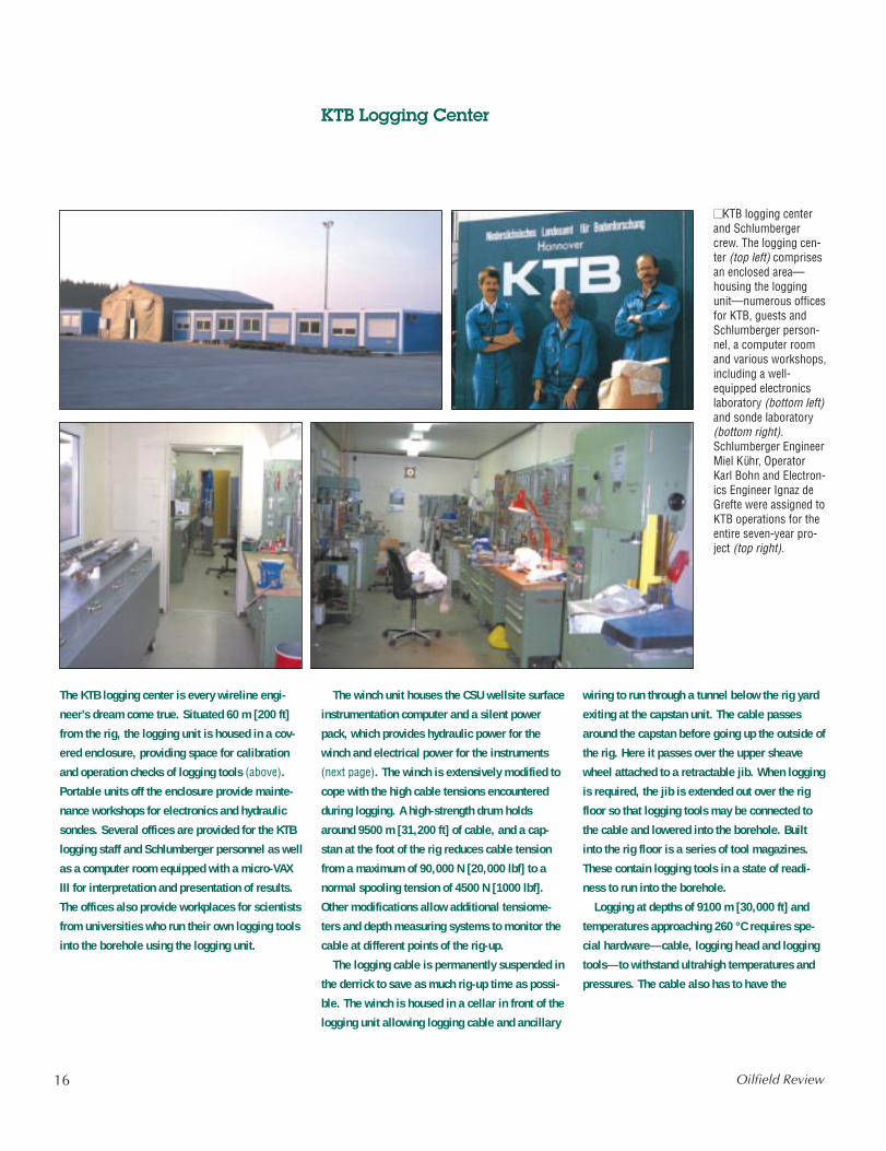
The KTB logging center is every wireline engi-
neer’s dream come true. Situated 60 m [200 ft]
from the rig, the logging unit is housed in a cov-
ered enclosure, providing space for calibration
and operation checks of logging tools (above).
Portable units off the enclosure provide mainte-
nance workshops for electronics and hydraulic
sondes. Several offices are provided for the KTB
logging staff and Schlumberger personnel as well
as a computer room equipped with a micro-VAX
III for interpretation and presentation of results.
The offices also provide workplaces for scientists
from universities who run their own logging tools
into the borehole using the logging unit.
The winch unit houses the CSU wellsite surface
instrumentation computer and a silent power
pack, which provides hydraulic power for the
winch and electrical power for the instruments
(next page). The winch is extensively modified to
cope with the high cable tensions encountered
during logging. A high-strength drum holds
around 9500 m [31,200 ft] of cable, and a cap-
stan at the foot of the rig reduces cable tension
from a maximum of 90,000 N [20,000 lbf] to a
normal spooling tension of 4500 N [1000 lbf].
Other modifications allow additional tensiome-
ters and depth measuring systems to monitor the
cable at different points of the rig-up.
The logging cable is permanently suspended in
the derrick to save as much rig-up time as possi-
ble. The winch is housed in a cellar in front of the
logging unit allowing logging cable and ancillary
wiring to run through a tunnel below the rig yard
exiting at the capstan unit. The cable passes
around the capstan before going up the outside of
the rig. Here it passes over the upper sheave
wheel attached to a retractable jib. When logging
is required, the jib is extended out over the rig
floor so that logging tools may be connected to
the cable and lowered into the borehole. Built
into the rig floor is a series of tool magazines.
These contain logging tools in a state of readi-
ness to run into the borehole.
Logging at depths of 9100 m [30,000 ft] and
temperatures approaching 260 °C requires spe-
cial hardware—cable, logging head and logging
tools—to withstand ultrahigh temperatures and
pressures. The cable also has to have the
16 Oilfield Review
■■KTB logging centerand Schlumbergercrew. The logging cen-ter (top left) comprisesan enclosed area—housing the loggingunit—numerous officesfor KTB, guests andSchlumberger person-nel, a computer roomand various workshops,including a well-equipped electronicslaboratory (bottom left)and sonde laboratory(bottom right). Schlumberger EngineerMiel Kühr, OperatorKarl Bohn and Electron-ics Engineer Ignaz deGrefte were assigned toKTB operations for theentire seven-year pro-ject (top right).
KTB Logging Center
strength to pull the logging tools back to surface.
At 9100 m, the normal logging tension is 67,000
N [15,000 lbf], right on the maximum safe pull for
the special high-strength cable used. This cable
has high-tensile steel armor wires and is thicker
than standard to provide the strength. It has spe-
cial insulating materials at the business end that
allow logging at temperatures up to 260 °C for
short periods of time.
If the borehole had gone any deeper, a two-
cable approach to logging would have been used.
At 10,000 m, the high-strength logging cable
would be in danger of breaking under its own
weight—even accounting for the buoyancy effect
of the mud. To reduce cable weight, a smaller
diameter, lighter, high-temperature cable hooked
up to a second winch would have been used to
lower logging tools into the borehole for the first
3200 m [10,500 ft]. At this depth, the small-
diameter cable would be connected to the high-
strength cable of the main winch and the journey
into the hole continued. With this tapered cable
configuration, the overall weight of cable is
decreased, reducing the tension, and the high-
strength cable is at the top of the hole where the
tension is greatest. This technique was used
twice, but only with 1500 m [4921 ft] of small-
diameter cable. This approach was taken by Rus-
sian well loggers to log the 12-km [7.4-mile]
Kola borehole using a three-conductor cable.
A special oil-filled logging head was developed
by Schlumberger for the KTB project. This had
high-temperature feed-throughs and special O-
rings, and provided the connection between cable
and logging tool.
Although there are several standard high-tem-
perature logging tools available, tools were
upgraded especially for KTB. One example is the
high-temperature Formation MicroScanner tool,
which was upgraded to 260 °C (next page, left).
The first task in modifying this tool was to pro-
duce a list of components to upgrade. Several
components, such as the pads containing the
button electrodes, were not changed, but could
be used only once. Other components, such as
the hydraulic motor that opens and closes the
sonde calipers, could still be used more than
once. Mechanical maintenance of such high-tem-
perature tools has to be meticulous—using even
one component that should have been changed
could result not only in a malfunction but also in
destruction of expensive equipment.
Temperature limits on the mechanical aspects
of the tool were relatively straightforward to over-
come. However, the electronics were of major
concern. Normally these operate up to 175 °C
17January 1995
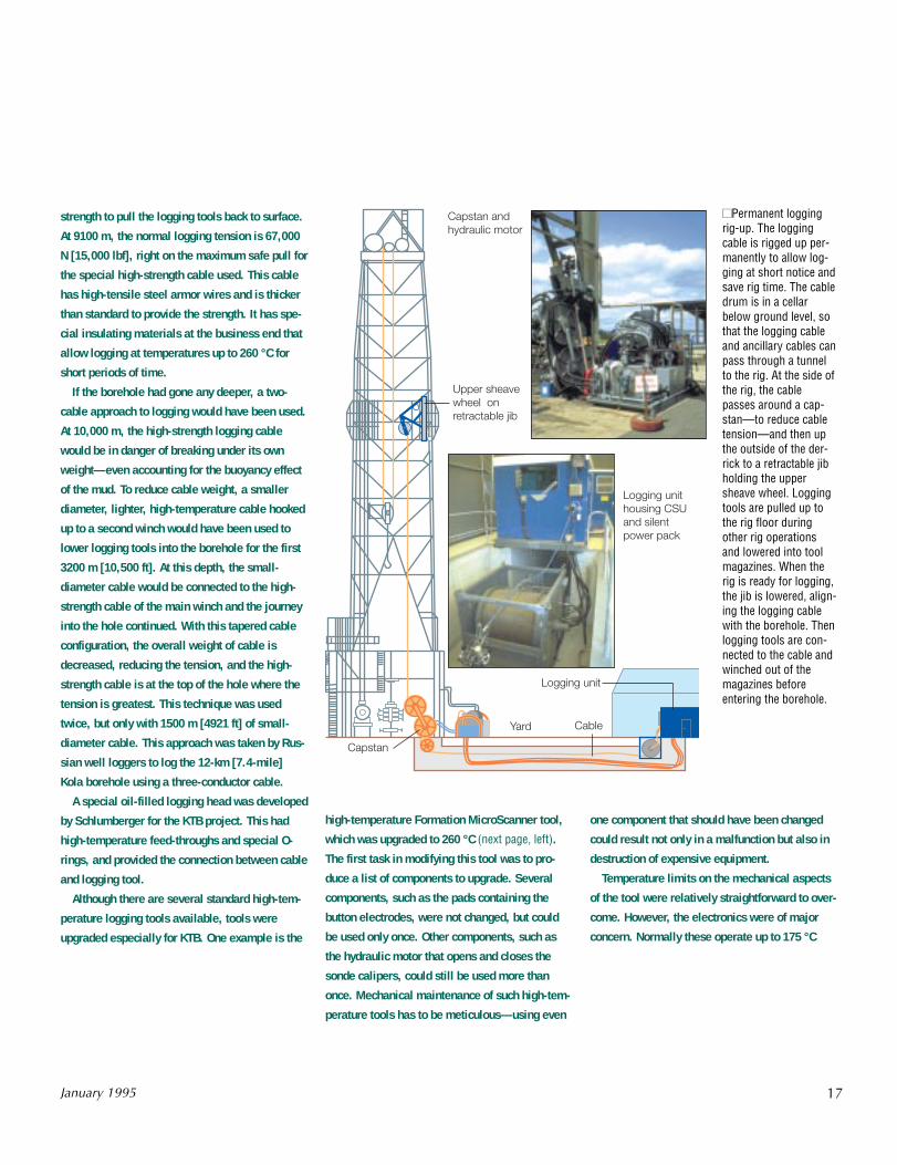
■■Permanent loggingrig-up. The loggingcable is rigged up per-manently to allow log-ging at short notice andsave rig time. The cabledrum is in a cellarbelow ground level, sothat the logging cableand ancillary cables canpass through a tunnelto the rig. At the side ofthe rig, the cablepasses around a cap-stan—to reduce cabletension—and then upthe outside of the der-rick to a retractable jibholding the uppersheave wheel. Loggingtools are pulled up tothe rig floor duringother rig operationsand lowered into toolmagazines. When therig is ready for logging,the jib is lowered, align-ing the logging cablewith the borehole. Thenlogging tools are con-nected to the cable andwinched out of themagazines beforeentering the borehole.
Capstan andhydraulic motor
Upper sheavewheel onretractable jib
Capstan
Yard
Logging unit
Cable
Logging unithousing CSUand silentpower pack
[350 °F]. To keep the temperature within this
limit meant housing them inside a Dewar flask
(below, right). The outside temperature could be
as high as 260 °C with the inside remaining
below 175 °C for up to 8 hours.
The cooling effects of mud circulation during
drilling were calculated to be about 50 °C [90 °F]
at TD. When circulation stopped, the temperature
would gradually climb, giving a window of 36
hours for logging before it exceeded tool ratings.
On the first logging run at TD, the maximum tem-
perature recorded was 240 °C [464 °F] and on
the last run, this reached 250.5 °C [483 °F]—
confirming earlier calculations. At the end of
each logging run the Dewar flasks were cooled
down slowly by blowing air through to avoid
thermal shock.
Apart from Schlumberger logging tools, sev-
eral universities developed equipment for their
own experiments in the borehole (see page 9).
18 Oilfield Review
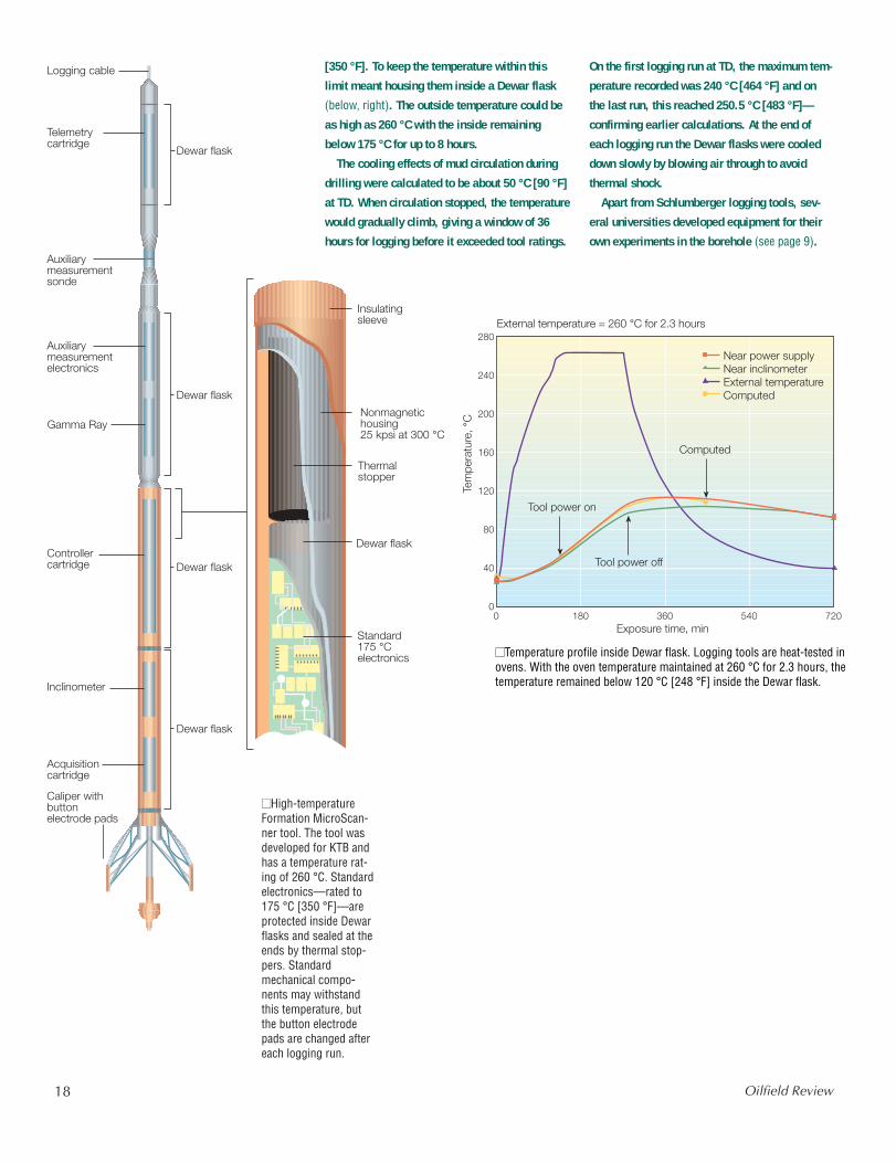
■■High-temperatureFormation MicroScan-ner tool. The tool wasdeveloped for KTB andhas a temperature rat-ing of 260 °C. Standardelectronics—rated to175 °C [350 °F]—areprotected inside Dewarflasks and sealed at theends by thermal stop-pers. Standardmechanical compo-nents may withstandthis temperature, butthe button electrodepads are changed aftereach logging run.
■■Temperature profile inside Dewar flask. Logging tools are heat-tested inovens. With the oven temperature maintained at 260 °C for 2.3 hours, thetemperature remained below 120 °C [248 °F] inside the Dewar flask.
External temperature = 260 °C for 2.3 hours
200
Tem
pera
ture
, °C
240
280
160
120
80
40
07205403601800
Near power supplyNear inclinometerExternal temperatureComputed
Tool power on
Tool power off
Computed
Exposure time, min
Logging cable
Telemetrycartridge
Auxiliarymeasurementsonde
Auxiliarymeasurementelectronics
Gamma Ray
Controllercartridge
Dewar flask
Inclinometer
Acquisitioncartridge
Caliper withbuttonelectrode pads
Insulatingsleeve
Nonmagnetichousing25 kpsi at 300 °C
Dewar flask
Standard175 °Celectronics
Thermalstopper
Dewar flask
Dewar flask
Dewar flask
Surprises—Some Welcome, Some NotBoth boreholes yielded unexpected resultsfor the scientists. Geologists had formed apicture of the crust at the Windischeschen-bach site by examining rock outcrops andtwo-dimensional (2D) seismic measure-ments. At a depth of about 7000 m[22,966 ft] they had expected to drillthrough the boundary between two tectonicplates that collided 320 million years ago,forming the Eurasian plate. However, thisboundary was never crossed, and the geolo-gists have had to redraw most of the subsur-face picture.
Other unexpected results include coreand log evidence for a network of conduc-tive pathways through highly resistive rock,and in rock devoid of matrix porosity, anample supply of water. Look at these find-ings in more detail:
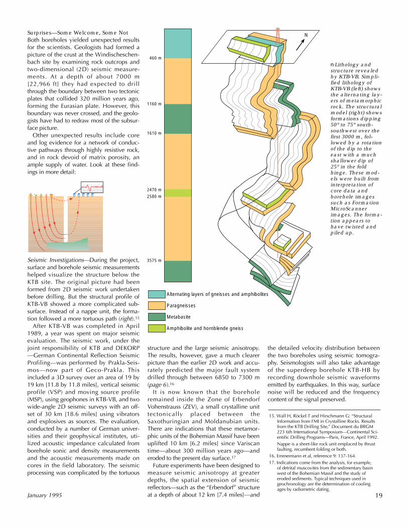
Seismic Investigations—During the project,surface and borehole seismic measurementshelped visualize the structure below theKTB site. The original picture had beenformed from 2D seismic work undertakenbefore drilling. But the structural profile ofKTB-VB showed a more complicated sub-surface. Instead of a nappe unit, the forma-tion followed a more tortuous path (right).15
After KTB-VB was completed in April1989, a year was spent on major seismicevaluation. The seismic work, under thejoint responsibility of KTB and DEKORP—German Continental Reflection SeismicProfiling—was performed by Prakla-Seis-mos—now part of Geco-Prakla. Thisincluded a 3D survey over an area of 19 by19 km [11.8 by 11.8 miles], vertical seismicprofile (VSP) and moving source profile(MSP), using geophones in KTB-VB, and twowide-angle 2D seismic surveys with an off-set of 30 km [18.6 miles] using vibratorsand explosives as sources. The evaluation,conducted by a number of German univer-sities and their geophysical institutes, uti-lized acoustic impedance calculated fromborehole sonic and density measurementsand the acoustic measurements made oncores in the field laboratory. The seismicprocessing was complicated by the tortuous
structure and the large seismic anisotropy.The results, however, gave a much clearerpicture than the earlier 2D work and accu-rately predicted the major fault systemdrilled through between 6850 to 7300 m(page 6).16
It is now known that the boreholeremained inside the Zone of ErbendorfVohenstrauss (ZEV), a small crystalline unittectonically placed between theSaxothuringian and Moldanubian units.There are indications that these metamor-phic units of the Bohemian Massif have beenuplifted 10 km [6.2 miles] since Variscantime—about 300 million years ago—anderoded to the present day surface.17
Future experiments have been designed tomeasure seismic anisotropy at greaterdepths, the spatial extension of seismicreflectors—such as the “Erbendorf” structureat a depth of about 12 km [7.4 miles]—andJanuary 1995
nLithology andstructure revealedby KTB-VB. Simpli-fied lithology ofKTB-VB (left) showsthe alternating lay-ers of metamorphicrock. The structuralmodel (right) showsformations dipping50° to 75° south-southwest over thefirst 3000 m, fol-lowed by a rotationof the dip to theeast with a muchshallower dip of25° in the foldhinge. These mod-els were built frominterpretation ofcore data andborehole imagessuch as FormationMicroScannerimages. The forma-tion appears tohave twisted andpiled up.
15. Wall H, Röckel T and Hirschmann G: “StructuralInformation from FMI in Crystalline Rocks. Resultsfrom the KTB Drilling Site,” Document du BRGM223 6th International Symposium—Continental Sci-entific Drilling Programs—Paris, France, April 1992.Nappe is a sheet-like rock unit emplaced by thrustfaulting, recumbent folding or both.
16. Emmermann et al, reference 9: 137-164.17. Indications come from the analysis, for example,
of detrital muscovites from the sedimentary basinwest of the Bohemian Massif and the study oferoded sediments. Typical techniques used ingeochronology are the determination of coolingages by radiometric dating.
the detailed velocity distribution betweenthe two boreholes using seismic tomogra-phy. Seismologists will also take advantageof the superdeep borehole KTB-HB byrecording downhole seismic waveformsemitted by earthquakes. In this way, surfacenoise will be reduced and the frequencycontent of the signal preserved.
19
N
460 m
1160 m
1610 m
2470 m
2580 m
3575 m
Alternating layers of gneisses and amphibolites
Paragneisses
Metabasite
Amphibolite and hornblende gneiss
1000 E
800 E
600 E
400 E
200 E
0 E
1000 S
800 S
600 S
400 S
200 S
0S
E2E3
E4
6000
4000
2000
0
m
KTB-VB
KTB-HB
4V
U22A
I
Polarity I + –Polarity II – +
Referenceelectrode KTB-VB
KTB-HB
E1
Naabdemnreuth
Nottersdorf
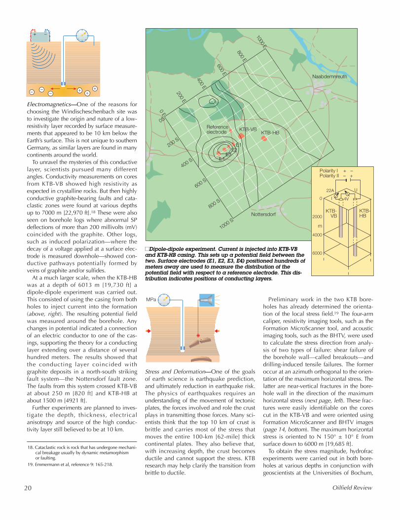
Electromagnetics—One of the reasons forchoosing the Windischeschenbach site wasto investigate the origin and nature of a low-resistivity layer recorded by surface measure-ments that appeared to be 10 km below theEarth’s surface. This is not unique to southernGermany, as similar layers are found in manycontinents around the world.
To unravel the mysteries of this conductivelayer, scientists pursued many differentangles. Conductivity measurements on coresfrom KTB-VB showed high resistivity asexpected in crystalline rocks. But then highlyconductive graphite-bearing faults and cata-clastic zones were found at various depthsup to 7000 m [22,970 ft].18 These were alsoseen on borehole logs where abnormal SPdeflections of more than 200 millivolts (mV)coincided with the graphite. Other logs,such as induced polarization—where thedecay of a voltage applied at a surface elec-trode is measured downhole—showed con-ductive pathways potentially formed byveins of graphite and/or sulfides.
At a much larger scale, when the KTB-HBwas at a depth of 6013 m [19,730 ft] adipole-dipole experiment was carried out.This consisted of using the casing from bothholes to inject current into the formation(above, right). The resulting potential fieldwas measured around the borehole. Anychanges in potential indicated a connectionof an electric conductor to one of the cas-ings, supporting the theory for a conductinglayer extending over a distance of severalhundred meters. The results showed thatthe conducting layer coincided withgraphite deposits in a north-south strikingfault system—the Nottersdorf fault zone.The faults from this system crossed KTB-VBat about 250 m [820 ft] and KTB-HB atabout 1500 m [4921 ft].
Further experiments are planned to inves-tigate the depth, thickness, electricalanisotropy and source of the high conduc-tivity layer still believed to be at 10 km.
Stress and Deformation—One of the goalsof earth science is earthquake prediction,and ultimately reduction in earthquake risk.The physics of earthquakes requires anunderstanding of the movement of tectonicplates, the forces involved and role the crustplays in transmitting those forces. Many sci-entists think that the top 10 km of crust isbrittle and carries most of the stress thatmoves the entire 100-km [62-mile] thickcontinental plates. They also believe that,with increasing depth, the crust becomesductile and cannot support the stress. KTBresearch may help clarify the transition frombrittle to ductile.
Preliminary work in the two KTB bore-holes has already determined the orienta-tion of the local stress field.19 The four-armcaliper, resistivity imaging tools, such as theFormation MicroScanner tool, and acousticimaging tools, such as the BHTV, were usedto calculate the stress direction from analy-sis of two types of failure: shear failure ofthe borehole wall—called breakouts—anddrilling-induced tensile failures. The formeroccur at an azimuth orthogonal to the orien-tation of the maximum horizontal stress. Thelatter are near-vertical fractures in the bore-hole wall in the direction of the maximumhorizontal stress (next page, left). These frac-tures were easily identifiable on the corescut in the KTB-VB and were oriented usingFormation MicroScanner and BHTV images(page 14, bottom). The maximum horizontalstress is oriented to N 150° ± 10° E fromsurface down to 6000 m [19,685 ft].
To obtain the stress magnitude, hydrofracexperiments were carried out in both bore-holes at various depths in conjunction withgeoscientists at the Universities of Bochum,
20 Oilfield Review
■■Dipole-dipole experiment. Current is injected into KTB-VBand KTB-HB casing. This sets up a potential field between thetwo. Surface electrodes (E1, E2, E3, E4) positioned hundreds ofmeters away are used to measure the distribution of thepotential field with respect to a reference electrode. This dis-tribution indicates positions of conducting layers.
18. Cataclastic rock is rock that has undergone mechani-cal breakage usually by dynamic metamorphism or faulting.
19. Emmermann et al, reference 9: 165-218.
+–
–– ++
–+
MPa
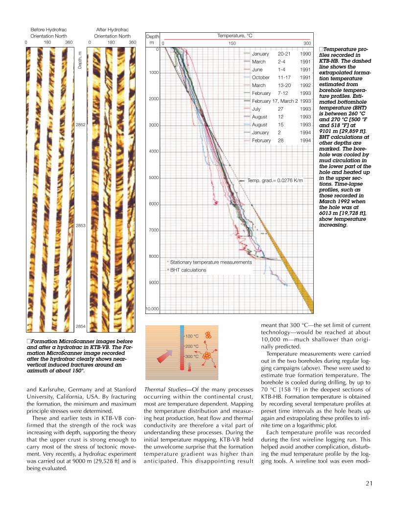
■■Formation MicroScanner images beforeand after a hydrofrac in KTB-VB. The For-mation MicroScanner image recordedafter the hydrofrac clearly shows near-vertical induced fractures around anazimuth of about 150°.
and Karlsruhe, Germany and at StanfordUniversity, California, USA. By fracturingthe formation, the minimum and maximumprinciple stresses were determined.
These and earlier tests in KTB-VB con-firmed that the strength of the rock wasincreasing with depth, supporting the theorythat the upper crust is strong enough tocarry most of the stress of tectonic move-ment. Very recently, a hydrofrac experimentwas carried out at 9000 m [29,528 ft] and isbeing evaluated.
Thermal Studies—Of the many processesoccurring within the continental crust,most are temperature dependent. Mappingthe temperature distribution and measur-ing heat production, heat flow and thermalconductivity are therefore a vital part ofunderstanding these processes. During theinitial temperature mapping, KTB-VB heldthe unwelcome surprise that the formationtemperature gradient was higher thananticipated. This disappointing result
21
■■Temperature pro-files recorded inKTB-HB. The dashedline shows theextrapolated forma-tion temperatureestimated from borehole tempera-ture profiles. Esti-mated bottomholetemperature (BHT) is between 260 °Cand 270 °C [500 °Fand 518 °F] at 9101 m [29,859 ft].BHT calculations atother depths aremarked. The bore-hole was cooled bymud circulation inthe lower part of thehole and heated upin the upper sec-tions. Time-lapseprofiles, such asthose recorded inMarch 1992 whenthe hole was at 6013 m [19,728 ft],show temperatureincreasing.
100 °C
200 °C
300 °C
meant that 300 °C—the set limit of currenttechnology—would be reached at about10,000 m—much shallower than origi-nally predicted.
Temperature measurements were carriedout in the two boreholes during regular log-ging campaigns (above). These were used toestimate true formation temperature. Theborehole is cooled during drilling, by up to70 °C [158 °F] in the deepest sections ofKTB-HB. Formation temperature is obtainedby recording several temperature profiles atpreset time intervals as the hole heats upagain and extrapolating these profiles to infi-nite time on a logarithmic plot.
Each temperature profile was recordedduring the first wireline logging run. Thishelped avoid another complication, disturb-ing the mud temperature profile by the log-ging tools. A wireline tool was even modi-
Orientation NorthAfter HydrofracBefore Hydrofrac
0 360180Orientation North
0 360180
2854
2853
2852
Dep
th, m
Depth m
Temperature, °C
10,000
9000
8000
7000
6000
5000
4000
3000
2000
1000
03001500
Temp. grad.= 0.0276 K/m
January 20-21 1990
March 2-4 1991
June 1-4 1991
October 11-17 1991
March 13-20 1992
February 7-12 1993
February 17, March 2 1993
July 27 1993
August 12 1993
August 15 1993
January 2 1994
February 28 1994
Stationary temperature measurements
BHT calculations
fied at KTB with the temperature sensormounted on the bottom of the tool to pro-vide the least disturbance and give the bestpossible result.
Temperature data provided an opportunityto measure heat production and conductiv-ity. In addition, thermal conductivity mea-surements were carried out in the field labo-ratory on cores cut from the boreholes.From the NGS and Litho-Density data, heatproduced by radioactive decay was calcu-lated—for metabasites the results were 0.5micro-Watts per cubic meter (µW/m3) andfor gneisses 1.6 µW/m3.
The final temperature profile has yet to beextrapolated from the data obtained so far.Experiments will continue to examine tem-perature distribution, heat production, heatflow and thermal conductivity.
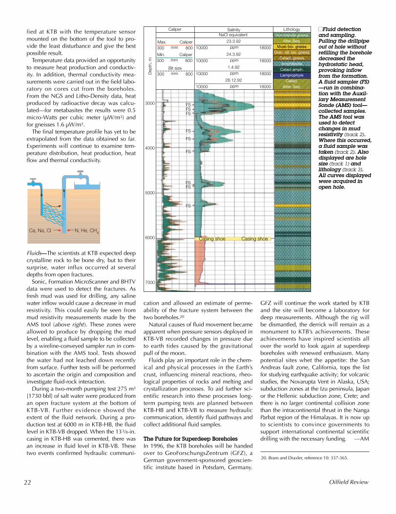
Fluids—The scientists at KTB expected deepcrystalline rock to be bone dry, but to theirsurprise, water influx occurred at severaldepths from open fractures.
Sonic, Formation MicroScanner and BHTVdata were used to detect the fractures. Asfresh mud was used for drilling, any salinewater inflow would cause a decrease in mudresistivity. This could easily be seen frommud resistivity measurements made by theAMS tool (above right). These zones wereallowed to produce by dropping the mudlevel, enabling a fluid sample to be collectedby a wireline-conveyed sampler run in com-bination with the AMS tool. Tests showedthe water had not leached down recentlyfrom surface. Further tests will be performedto ascertain the origin and composition andinvestigate fluid-rock interaction.
During a two-month pumping test 275 m3
[1730 bbl] of salt water were produced froman open fracture system at the bottom ofKTB-VB. Further evidence showed theextent of the fluid network. During a pro-duction test at 6000 m in KTB-HB, the fluidlevel in KTB-VB dropped. When the 133/8-in.casing in KTB-HB was cemented, there wasan increase in fluid level in KTB-VB. Thesetwo events confirmed hydraulic communi-
cation and allowed an estimate of perme-ability of the fracture system between thetwo boreholes.20
Natural causes of fluid movement becameapparent when pressure sensors deployed inKTB-VB recorded changes in pressure dueto earth tides caused by the gravitationalpull of the moon.
Fluids play an important role in the chem-ical and physical processes in the Earth’scrust, influencing mineral reactions, rheo-logical properties of rocks and melting andcrystallization processes. To aid further sci-entific research into these processes long-term pumping tests are planned betweenKTB-HB and KTB-VB to measure hydrauliccommunication, identify fluid pathways andcollect additional fluid samples.
The Future for Superdeep BoreholesIn 1996, the KTB boreholes will be handedover to GeoForschungsZentrum (GFZ), aGerman government-sponsored geoscien-tific institute based in Potsdam, Germany.
GFZ will continue the work started by KTBand the site will become a laboratory fordeep measurements. Although the rig willbe dismantled, the derrick will remain as amonument to KTB’s achievements. Theseachievements have inspired scientists allover the world to look again at superdeepboreholes with renewed enthusiasm. Manypotential sites whet the appetite: the SanAndreas fault zone, California, tops the listfor studying earthquake activity; for volcanicstudies, the Novarupta Vent in Alaska, USA;subduction zones at the Izu peninsula, Japanor the Hellenic subduction zone, Crete; andthere is no larger continental collision zonethan the intracontinental thrust in the NangaParbat region of the Himalayas. It is now upto scientists to convince governments tosupport international continental scientificdrilling with the necessary funding. —AM
22 Oilfield Review
■■Fluid detectionand sampling.Pulling the drillpipeout of hole withoutrefilling the boreholedecreased thehydrostatic head,provoking inflowfrom the formation.A fluid sampler (FS)—run in combina-tion with the Auxil-iary MeasurementSonde (AMS) tool—collected samples.The AMS tool wasused to detectchanges in mudresistivity (track 2).Where this occurred,a fluid sample wastaken (track 2). Also displayed are holesize (track 1) andlithology (track 3).All curves displayedwere acquired inopen hole.
Ca, Na, Cl N, He, CH4
Salinity
Dep
th, m
7000
6000
5000
4000
3000
300 800
Caliper
Max. Calipermm 10000 18000
23.3.92ppm
NaCl equivalent
10000 18000
24.3.92ppm
10000 18000
1.4.92ppm
10000 18000
28.12.92ppm
300 800Min. Caliper
mm
300 800Bit size
mm
FSFSFS
FS
FS
FS
FSFS
FS
Casing shoe Casing shoe
LithologyHornblende gneiss
Alter. Seq.
Musk bio. gneiss
Gran. sill. bio. gneiss
Catacl. gneiss
Amphibolite
Catacl amph.
Lamprophyre
Catacl.
Alter. Seq.
20. Bram and Draxler, reference 10: 337-365.
January 1995
For help in preparation of this article, thanBiro, Geco-Prakla, Dallas, Texas; Adrian BBrook and Colin Hulme, Geco-Prakla, Galand; Helge Bragstad, Peter Canter, Olav LOdd Olav Vatne, Geco-Prakla, Sandvika, Chapman, Conoco Inc., Ponca City, OklahKim El-Tawil, Tom Neugebauer and Mike Geco-Prakla, Houston, Texas; Bill Fraser aton, Hunt Oil Company, Dallas, Texas; JakPer Helgaker, Hans Klaassen, Dietmar KluSchnellbacher, Tony Woolmer and Mike W
Imagine breaking your leg image won’t be ready for interpretation
for a year or more. Until re r delays. But thanks to breakthroughs
in acquisition, processing time—time from the first shot to the
beginning of interpretatio
Chris BeckettTim BrooksGregg ParkerHouston, Texas, USA
Robin BjoroyDominique PajotPaul TaylorGatwick, England
David DeitzUnocalLafayette, Louisiana, USA
Terje FlatenLars Jan JaarvikStatoilStavanger, Norway
Ian JackKeith NunnBP ExplorationStockley Park, England
Alan StrudleyRobin WalkerStavanger, Norway
Reducing 3D Seismic Turnaround
ro-D
ledas isg-hefit.is- inowny
aser-nddeci-ceeyer-ithing
ingona-
tion. Unlike 2D seismic, which grew fromthe exploration market into development,3D seismic has grown in the opposite direc-tion. Companies are discovering that earlyacquisition of 3D data reduces finding costsand overall project costs.2 Interpreted seis-mic data are essential for intelligent biddingon acreage. And some exploration contractsnow require a 3D survey before drilling.This expansion into exploration, along withdecreases in the cost of seismic acquisitionand processing, has raised demand for 3Dseismic data.
This increased demand has forced servicecompanies to reduce turnaround time—without sacrificing quality. This article looksfirst at the dramatic improvements in marineturnaround time, then at the steps beingtaken to significantly reduce turnaround intransition zone and land surveys.
The Marine StoryThree years ago, a marine survey of 500 km2
[193 sq miles] took a year or more to beacquired and processed. Today, through acombination of new technologies, turn-around time for similar surveys can be as lit-
1. For the purpose of this article, 3D turnaround time isdefined as the time from first shot to the end of pro-cessing. Some companies use the term “cycle time.”Oil companies include the survey planning beforeacquisition and the interpretation after processing,
o,
-
.
SEISMICS
ks to Garyligh, Scipiotwick, Eng-indtjorn and
Norway; Bill
and having an X-ray, only to be told that the
cently, seismic surveys suffered from simila
and communication, 3D seismic turnaround
n—has been reduced from years to weeks.
There are two main reasons oil and gas pducers worry about the time spent on 3seismic acquisition and processing, calturnaround time.1 First, in the oil and gbusiness, as in every business, timemoney. The more time spent on drilling, loging and well completion, the longer tdelay in production and the lower the proAdd the time to acquire and interpret semic data before drilling, and the delaybringing reserves to the surface may grbeyond the schedules and budgets of maproduction managers.
Second, and special to the oil and gbusiness, saving time can make the diffence between being able to do business anot. Development contracts worldwirequire oil companies to drill within a spefied time. The clock starts ticking onacreage is licensed. A 3D seismic survplanned, acquired, processed and intpreted in advance arms developers wtools for intelligent well placement, yieldhigher production from fewer wells.
More 3D seismic surveys are also becommissioned for exploration, in additito field development, their initial applic
Geco-Prakla, Hannover, Germany; Hal Harper, ConocMidland, Texas; David Etherington-Brown, JohannesHvidsten and Phil Selley, Geco-Prakla, Stavanger, Norway; Kristian Kolbjørnsen, Saga Petroleum, Sandvika,Norway; Bård Krokan, Norsk Hydro, Stabekk, Norway
23
oma, USA;Spradley,nd Bruce Hin-ob Haldorsen,ge, Clausorthington,
so their turnaround time is from decision to shoot toselection of drillsite. However, planning and interpre-tation are often outside the responsibility of servicecompanies, so they remain outside the definition used here.
2. Chisolm G: “Advances in Delivering 3D Data to Customers,” presented at the PETEX 94 meeting onTechniques For Cost-Effective Exploration & Produc-tion, London, England, November 16-18, 1994.
In this article, Charisma, Digiseis-FLX, LINK, Monowing,Olympus-IMS, TQ3D, TRILOGY, TRINAV, TRIPRO,TRISOR and Voyager are marks of Schlumberger. RISC6000 is a mark of International Business Machines Cor-poration. SPARCstation 20 is a mark of Sun Microsys-tems, Inc.
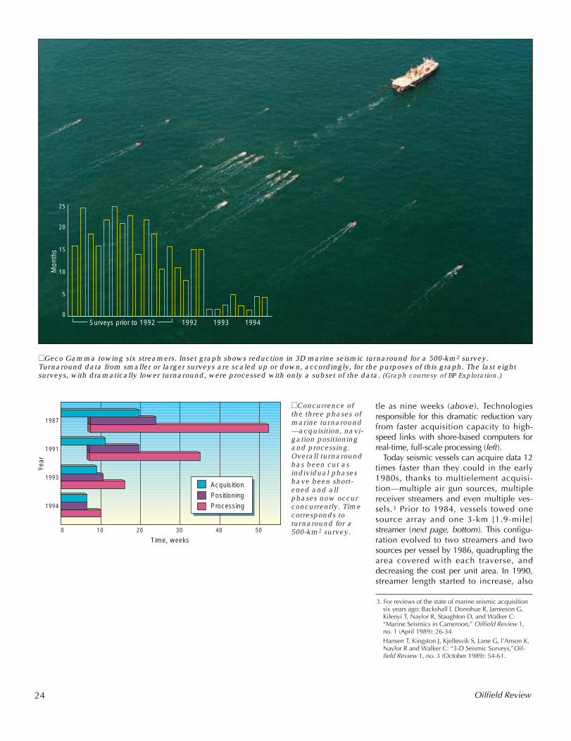
tle as nine weeks (above). Technologiesresponsible for this dramatic reduction varyfrom faster acquisition capacity to high-speed links with shore-based computers forreal-time, full-scale processing (left).
Today seismic vessels can acquire data 12times faster than they could in the early1980s, thanks to multielement acquisi-tion—multiple air gun sources, multiplereceiver streamers and even multiple ves-sels.3 Prior to 1984, vessels towed onesource array and one 3-km [1.9-mile]streamer (next page, bottom). This configu-ration evolved to two streamers and twosources per vessel by 1986, quadrupling thearea covered with each traverse, anddecreasing the cost per unit area. In 1990,streamer length started to increase, also
24 Oilfield Review
■■Concurrence ofthe three phases ofmarine turnaround—acquisition, navi-gation positioningand processing.Overall turnaroundhas been cut asindividual phaseshave been short-ened and allphases now occurconcurrently. Timecorresponds toturnaround for a500-km2 survey.
■■Geco Gamma towing six streamers. Inset graph shows reduction in 3D marine seismic turnaround for a 500-km2 survey.Turnaround data from smaller or larger surveys are scaled up or down, accordingly, for the purposes of this graph. The last eightsurveys, with dramatically lower turnaround, were processed with only a subset of the data. (Graph courtesy of BP Exploration.)
3. For reviews of the state of marine seismic acquisitionsix years ago: Backshall l, Donohue R, Jamieson G,Kilenyi T, Naylor R, Staughton D, and Walker C:“Marine Seismics in Cameroon,” Oilfield Review 1,no. 1 (April 1989): 26-34.Hansen T, Kingston J, Kjellesvik S, Lane G, l’Anson K,Naylor R and Walker C: “3-D Seismic Surveys,”Oil-field Review 1, no. 3 (October 1989): 54-61.
Aquisition
Positioning
Processing
Year
1987
1991
1993
1994
Time, weeks50403020100
Acquisition
Positioning
Processing
Surveys prior to 1992 1992 1993 1994
25
20
15
10
5
0
Mon
ths
decreasing costs. By 1991, there were twosources firing alternately to three streamers,and by 1992, there were four streamers. In1994, the Geco Gamma acquired theworld’s first survey with six streamers. Andin a continuing quest for greater capacity,contractors are now building or refurbishingseismic vessels to tow 8 to 12 streamers.
A challenge in designing vessels for multi-streamer acquisition is to keep all thestreamers uniformly separated while main-taining vessel speed. Streamers are sepa-rated with a deflector, which steers outerstreamers away from their normal streamlines (right). Most streamers follow angledslabs—paravanes—which deflect thestreamer outward, but also create drag onthe vessel. Each 3-km deflected streamermay exert up to 12 tons of drag, forcing thevessel to consume more fuel to maintainspeed. Eight to twelve streamers, with para-vanes deflecting the outer ones, would actlike a sea anchor, creating enough drag tostop an ordinary vessel. One contractor,PGS Exploration, is designing a more pow-erful vessel to address this problem.
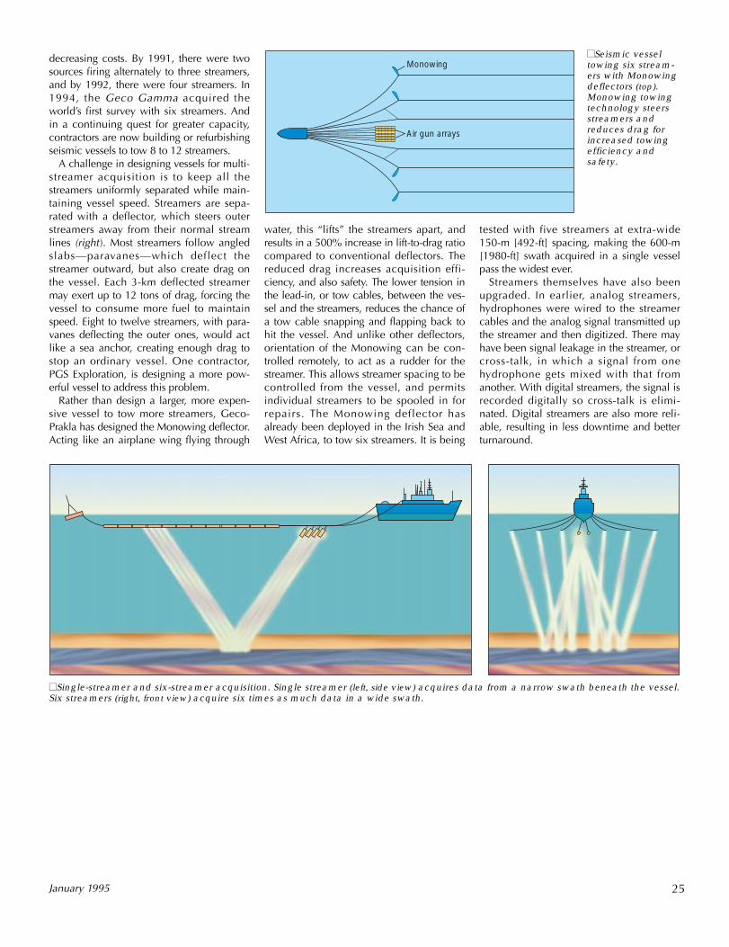
Rather than design a larger, more expen-sive vessel to tow more streamers, Geco-Prakla has designed the Monowing deflector.Acting like an airplane wing flying through
25January 1995
■■Seismic vesseltowing six stream-ers with Monowingdeflectors (top).Monowing towingtechnology steersstreamers andreduces drag forincreased towingefficiency andsafety.
■■Single-streamer and six-streamer acquisition. Single streamer (left, side view) acquires data from a narrow swath beneath the vessel.Six streamers (right, front view) acquire six times as much data in a wide swath.
Monowing
Air gun arrays
water, this “lifts” the streamers apart, andresults in a 500% increase in lift-to-drag ratiocompared to conventional deflectors. Thereduced drag increases acquisition effi-ciency, and also safety. The lower tension inthe lead-in, or tow cables, between the ves-sel and the streamers, reduces the chance ofa tow cable snapping and flapping back tohit the vessel. And unlike other deflectors,orientation of the Monowing can be con-trolled remotely, to act as a rudder for thestreamer. This allows streamer spacing to becontrolled from the vessel, and permitsindividual streamers to be spooled in forrepairs. The Monowing deflector hasalready been deployed in the Irish Sea andWest Africa, to tow six streamers. It is being
tested with five streamers at extra-wide150-m [492-ft] spacing, making the 600-m[1980-ft] swath acquired in a single vesselpass the widest ever.
Streamers themselves have also beenupgraded. In earlier, analog streamers,hydrophones were wired to the streamercables and the analog signal transmitted upthe streamer and then digitized. There mayhave been signal leakage in the streamer, orcross-talk, in which a signal from onehydrophone gets mixed with that fromanother. With digital streamers, the signal isrecorded digitally so cross-talk is elimi-nated. Digital streamers are also more reli-able, resulting in less downtime and betterturnaround.
While multielement acquisition hasplayed the leading role in reducing acquisi-tion time, it has created a new challenge inreducing overall turnaround time. Data canarrive at a staggering 5 MBytes/sec andsome of it must be processed before thenext shot is fired—about every 10 seconds—if the processing is to keep pace. Rising tothe challenge is concurrent processing, acombination of onboard processing andhigh-speed communication with onshorecomputers and decision makers.
To achieve minimum turnaround time,two sets of data—source signature qualityand survey position—must be processedbetween shots. The source is a cluster of dif-ferent-sized air guns. On Geco-Prakla ves-sels the air guns are controlled by theTRISOR module of the TRILOGY integratedacquisition and processing system. Thismodule fires the air guns in a sequence thatis tuned to their sizes. As the size of the gunincreases, so does the time from firing tomaximum pressure. The TRISOR controllersynchronizes the guns’ pressure maxima,giving a stronger source signal.
TRISOR hardware also monitors sourceoutput to check the quality of each shot.
TRISOR sensors, located within one meterof the air guns, communicate with the ves-sel through fiber-optic connections, and arepackaged based on concepts from Anadrill’smeasurements-while-drilling (MWD) tech-nology. In this hostile environment, near ahigh-energy source and sustaining at least500,000 shocks per year, the rugged con-struction that ensures reliable MWD alsohelps reduce seismic turnaround.
To maximize vessel uptime, errors such asa gun going off at the wrong time, or not atall, must be detected immediately. Thenprocessing specialists can determinewhether the shot must be retaken, orwhether the recorded signal satisfies thegeophysical objectives of the survey. If thesignal is sufficient, time is saved. If insuffi-cient, time is still saved, because a seismicline can be quickly reshot while the vessel isstill over the survey area.
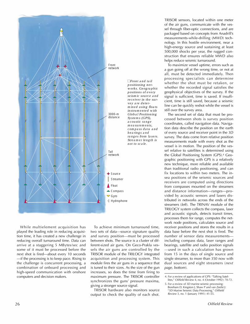
The second set of data that must be pro-cessed between shots is survey positioncoordinates, called navigation data. Naviga-tion data describe the position on the earthof every source and receiver point in the 3Dsurvey. The data come from relative positionmeasurements made with every shot as thevessel is in motion. The position of the ves-sel relative to satellites is determined usingthe Global Positioning System (GPS).4 Geo-graphic positioning with GPS is a relativelynew technique, more reliable and availablethan traditional radio positioning, and canfix locations to within two meters. The in-sea positions of the seismic sources andreceivers are computed using directionsfrom compasses mounted on the streamersand distance information—ranges—pro-vided by acoustic sensors and lasers dis-tributed in networks across the ends of thestreamers (left). The TRINAV module of theTRILOGY system collects the compass, laserand acoustic signals, detects transit times,processes them for range, computes the net-work node positions, calculates source andreceiver positions and stores the results in adata base before the next shot is fired. Thenumber of sensor data measurements—including compass data, laser ranges andbearings, satellite and radio position signals—used in such a calculation has grownfrom 15 in the days of single source andsingle streamer, to more than 350 now withdual sources and eight streamers (nextpage, bottom).
■■Front and tailpositioning net-works. Geographicpositions of everyseismic source andreceiver in the sur-vey are deter-mined using floatsinstrumented withGlobal PositioningSystems (GPS),acoustic rangemeasurements,compass data andbearings andranges from lasers.Streamer length isnot to scale.
Oilfield Review
4. For a review of applications of GPS: “Talking Satel-lites,” Oilfield Review 4, no. 4 (October 1992): 70-72.
5. For a review of 3D marine seismic processing: Boreham D, Kingston J, Shaw P and van Zeelst J: “3D Marine Seismic Data Processing,” OilfieldReview 3, no. 1 (January 1991): 41-55.
Source
Tailnetwork
3000-mdistance
Frontnetwork
Streamer
Float
Compass
Gyro
Hydrophone
26
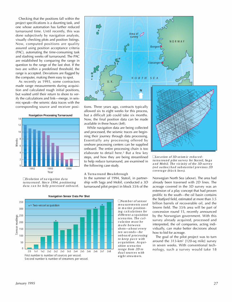
N O R W A Y
Bergen
Stavanger
N O R T H S E A
Area ofsurvey
U. K.
N
■■Evolution of navigation dataturnaround. Since 1994, positioningdata can be fully processed onboard.
■■Location of 3D seismic reduced-turnaround pilot survey for Statoil, Sagaand Mobil. The vicinity of the 3D survey(red outline) had substantial previous 2Dcoverage (black lines).
■■Number of sensormeasurements usedin marine position-ing calculations fordifferent acquisitionscenarios. The cal-culation must bemade betweenshots—about everyten seconds—foronboard processingto keep pace withacquisition. Acqui-sition scenariosrange from 2D todual sources witheight streamers.
27January 1995
Checking that the positions fall within theproject specifications is a daunting task, andone whose automation has further reducedturnaround time. Until recently, this wasdone subjectively by navigation analysts,visually checking plots and position listings.Now, computed positions are qualityassured using position acceptance criteria(PAC), automating the time-consuming taskand slashing weeks off turnaround. The PACare established by comparing the range inquestion to the range of the last shot. If thetwo are within a predefined threshold, therange is accepted. Deviations are flagged bythe computer, making them easy to spot.
As recently as 1993, some contractorsmade range measurements during acquisi-tion and calculated rough initial positions,but waited until their return to shore to ver-ify the calculations and link—merge, in seis-mic-speak—the seismic data traces with thecorresponding source and receiver posi- tions. Three years ago, contracts typically
allowed six to eight weeks for this process,but a difficult job could take six months.Now, the final position data can be madeavailable in three hours (left).
While navigation data are being collectedand processed, the seismic traces are begin-ning their journey through data processing.Essentially any processing offered byonshore processing centers can be suppliedonboard. The entire processing chain is tooelaborate to detail here.5 But a few keysteps, and how they are being streamlinedto help reduce turnaround, are examined inthe following case study.
A Turnaround BreakthroughIn the summer of 1994, Statoil, in partner-ship with Saga and Mobil, conducted a 3Dturnaround pilot project in block 33/6 of the
Norwegian North Sea (above). The area hadalready been traversed with 2D lines. Theacreage covered in the 3D survey was anextension of a play concept that had provenprolific to the south—the oil basin containsthe Statfjord field, estimated at more than 3.5billion barrels of recoverable oil, and theSnorre field. The 33/6 area will be part ofconcession round 15, recently announcedby the Norwegian government. With thissurvey already acquired, processed andinterpreted, the oil companies, acting indi-vidually, can make better decisions abouthow to bid for acreage.
The goal of the pilot project was to turnaround the 313-km2 [120-sq mile] surveyin seven weeks. With conventional tech-nology, such a survey would take 18
1992 1993 19940
2
4
6
8
10
12
Year
Wee
ks
Navigation Processing Turnaround14
Navigation Sensor Data Per Shot
Sen
sor
read
ings
350
300
250
200
150
100
50
02x21x21x12D 2x2 2x3 2x4 2x5 2x6 2x6 2x73x3 2x8
*
*** = Two-vessel acquisition
First number is number of sources per vessel.Second number is number of streamers per vessel.
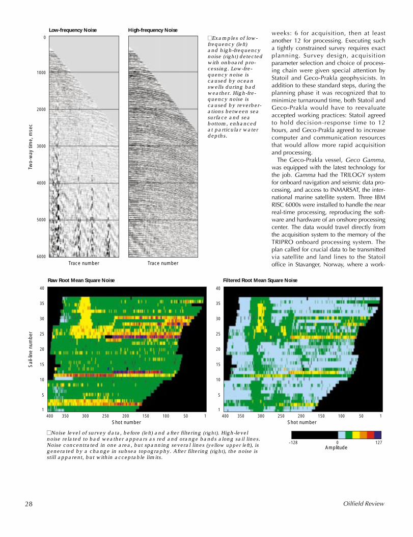
weeks: 6 for acquisition, then at leastanother 12 for processing. Executing sucha tightly constrained survey requires exactplanning. Survey design, acquisitionparameter selection and choice of process-ing chain were given special attention byStatoil and Geco-Prakla geophysicists. Inaddition to these standard steps, during theplanning phase it was recognized that tominimize turnaround time, both Statoil andGeco-Prakla would have to reevaluateaccepted working practices: Statoil agreedto hold decision-response time to 12hours, and Geco-Prakla agreed to increasecomputer and communication resourcesthat would allow more rapid acquisitionand processing.
The Geco-Prakla vessel, Geco Gamma,was equipped with the latest technology forthe job. Gamma had the TRILOGY systemfor onboard navigation and seismic data pro-cessing, and access to INMARSAT, the inter-national marine satellite system. Three IBMRISC 6000s were installed to handle the nearreal-time processing, reproducing the soft-ware and hardware of an onshore processingcenter. The data would travel directly fromthe acquisition system to the memory of theTRIPRO onboard processing system. Theplan called for crucial data to be transmittedvia satellite and land lines to the Statoiloffice in Stavanger, Norway, where a work-
28 Oilfield Review
■■Noise level of survey data, before (left) and after filtering (right). High-levelnoise related to bad weather appears as red and orange bands along sail lines.Noise concentrated in one area, but spanning several lines (yellow upper left), isgenerated by a change in subsea topography. After filtering (right), the noise isstill apparent, but within acceptable limits.
■■Examples of low-frequency (left)and high-frequencynoise (right) detectedwith onboard pro-cessing. Low-fre-quency noise iscaused by oceanswells during badweather. High-fre-quency noise iscaused by reverber-ations between seasurface and seabottom, enhanced at particular waterdepths.
6000
1000
0
2000
3000
4000
5000
Trace number Trace number
Two-
way
tim
e, m
sec
Low-frequency Noise High-frequency Noise
400 350 300
-128 1270
250 200 150 100 50
10
15
20
25
30
35
40
5
11
10
15
20
25
30
35
40
5
1
Shot number400 350 300 250 200 150 100 50 1
Shot number
Amplitude
Sai
l-lin
e nu
mbe
r
Filtered Root Mean Square NoiseRaw Root Mean Square Noise
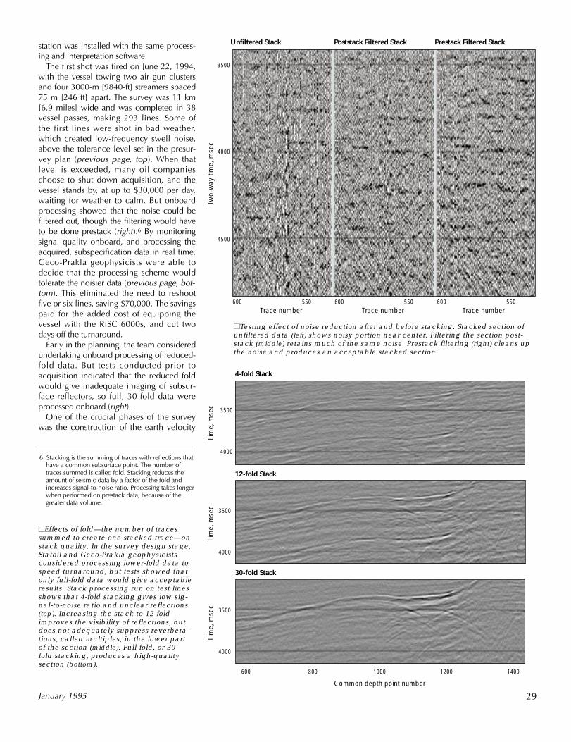
29January 1995
station was installed with the same process-ing and interpretation software.
The first shot was fired on June 22, 1994,with the vessel towing two air gun clustersand four 3000-m [9840-ft] streamers spaced75 m [246 ft] apart. The survey was 11 km[6.9 miles] wide and was completed in 38vessel passes, making 293 lines. Some ofthe first lines were shot in bad weather,which created low-frequency swell noise,above the tolerance level set in the presur-vey plan (previous page, top). When thatlevel is exceeded, many oil companieschoose to shut down acquisition, and thevessel stands by, at up to $30,000 per day,waiting for weather to calm. But onboardprocessing showed that the noise could befiltered out, though the filtering would haveto be done prestack (right).6 By monitoringsignal quality onboard, and processing theacquired, subspecification data in real time,Geco-Prakla geophysicists were able todecide that the processing scheme wouldtolerate the noisier data (previous page, bot-tom). This eliminated the need to reshootfive or six lines, saving $70,000. The savingspaid for the added cost of equipping thevessel with the RISC 6000s, and cut twodays off the turnaround.
Early in the planning, the team consideredundertaking onboard processing of reduced-fold data. But tests conducted prior toacquisition indicated that the reduced foldwould give inadequate imaging of subsur-face reflectors, so full, 30-fold data wereprocessed onboard (right).
One of the crucial phases of the surveywas the construction of the earth velocity
■■Testing effect of noise reduction after and before stacking. Stacked section ofunfiltered data (left) shows noisy portion near center. Filtering the section post-stack (middle) retains much of the same noise. Prestack filtering (right) cleans upthe noise and produces an acceptable stacked section.
■■Effects of fold—the number of tracessummed to create one stacked trace—onstack quality. In the survey design stage,Statoil and Geco-Prakla geophysicistsconsidered processing lower-fold data tospeed turnaround, but tests showed thatonly full-fold data would give acceptableresults. Stack processing run on test linesshows that 4-fold stacking gives low sig-nal-to-noise ratio and unclear reflections(top). Increasing the stack to 12-foldimproves the visibility of reflections, butdoes not adequately suppress reverbera-tions, called multiples, in the lower partof the section (middle). Full-fold, or 30-fold stacking, produces a high-qualitysection (bottom).
6. Stacking is the summing of traces with reflections thathave a common subsurface point. The number oftraces summed is called fold. Stacking reduces theamount of seismic data by a factor of the fold andincreases signal-to-noise ratio. Processing takes longerwhen performed on prestack data, because of thegreater data volume.
Two-
way
tim
e, m
sec
Unfiltered Stack Poststack Filtered Stack Prestack Filtered Stack
4500
4000
3500
600 550600 550 600 550Trace number Trace number Trace number
4000
600 800 1000 1200 1400
3500
Common depth point number
Tim
e, m
sec
Tim
e, m
sec
Tim
e, m
sec
4-fold Stack
12-fold Stack
30-fold Stack
4000
3500
4000
3500
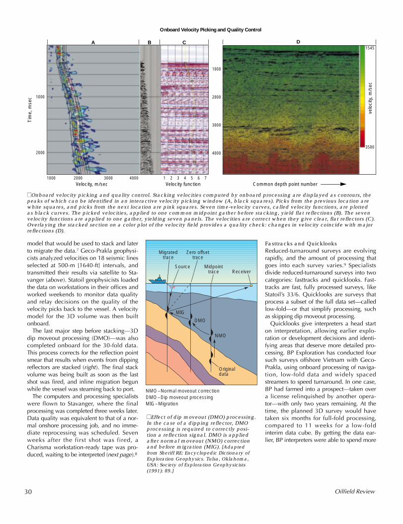
model that would be used to stack and laterto migrate the data.7 Geco-Prakla geophysi-cists analyzed velocities on 18 seismic linesselected at 500-m [1640-ft] intervals, andtransmitted their results via satellite to Sta-vanger (above). Statoil geophysicists loadedthe data on workstations in their offices andworked weekends to monitor data qualityand relay decisions on the quality of thevelocity picks back to the vessel. A velocitymodel for the 3D volume was then builtonboard.
The last major step before stacking—3Ddip moveout processing (DMO)—was alsocompleted onboard for the 30-fold data.This process corrects for the reflection pointsmear that results when events from dippingreflectors are stacked (right). The final stackvolume was being built as soon as the lastshot was fired, and inline migration begunwhile the vessel was steaming back to port.
The computers and processing specialistswere flown to Stavanger, where the finalprocessing was completed three weeks later.Data quality was equivalent to that of a nor-mal onshore processing job, and no imme-diate reprocessing was scheduled. Sevenweeks after the first shot was fired, aCharisma workstation-ready tape was pro-duced, waiting to be interpreted (next page).8
Fasttracks and QuicklooksReduced-turnaround surveys are evolvingrapidly, and the amount of processing thatgoes into each survey varies.9 Specialistsdivide reduced-turnaround surveys into twocategories: fasttracks and quicklooks. Fast-tracks are fast, fully processed surveys, likeStatoil’s 33/6. Quicklooks are surveys thatprocess a subset of the full data set—calledlow-fold—or that simplify processing, suchas skipping dip moveout processing.
Quicklooks give interpreters a head starton interpretation, allowing earlier explo-ration or development decisions and identi-fying areas that deserve more detailed pro-cessing. BP Exploration has conducted foursuch surveys offshore Vietnam with Geco-Prakla, using onboard processing of naviga-tion, low-fold data and widely spacedstreamers to speed turnaround. In one case,BP had farmed into a prospect—taken overa license relinquished by another opera-tor—with only two years remaining. At thetime, the planned 3D survey would havetaken six months for full-fold processing,compared to 11 weeks for a low-foldinterim data cube. By getting the data ear-lier, BP interpreters were able to spend more
30 Oilfield Review
■■Onboard velocity picking and quality control. Stacking velocities computed by onboard processing are displayed as contours, thepeaks of which can be identified in an interactive velocity picking window (A, black squares). Picks from the previous location arewhite squares, and picks from the next location are pink squares. Seven time-velocity curves, called velocity functions, are plottedas black curves. The picked velocities, applied to one common midpoint gather before stacking, yield flat reflections (B). The sevenvelocity functions are applied to one gather, yielding seven panels. The velocities are correct when they give clear, flat reflectors (C).Overlaying the stacked section on a color plot of the velocity field provides a quality check: changes in velocity coincide with majorreflections (D).
■■Effect of dip moveout (DMO) processing.In the case of a dipping reflector, DMOprocessing is required to correctly posi-tion a reflection signal. DMO is appliedafter normal moveout (NMO) correctionand before migration (MIG). [Adaptedfrom Sheriff RE: Encyclopedic Dictionary ofExploration Geophysics. Tulsa, Oklahoma,USA: Society of Exploration Geophysicists(1991): 89.]
NMO
DMO
MIG
Source Midpointtrace Receiver
Zero offsettrace
Migratedtrace
Originaldata
NMO–Normal moveout correctionDMO–Dip moveout processingMIG–Migration
2000
1000
2000
3000
4000
1000
Velocity, m/sec Velocity function Common depth point number
Tim
e, m
sec
Onboard Velocity Picking and Quality Control
1545
3500
1000 2000 3000 4000 1 2 3 4 5 6 7
velo
city
, m/s
ec
DCBA
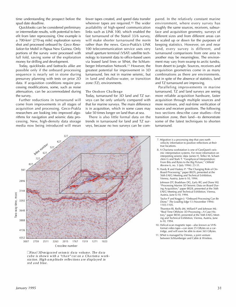
pared. In the relatively constant marineenvironment, where every survey hasroughly the same sources, receivers, subsur-face and acquisition geometry, surveys ofdifferent sizes and from different areas canbe scaled up or down for the purposes ofkeeping statistics. However, on and nearland, every survey is different, andturnaround comparisons from one area toanother may be meaningless. The environ-ment may vary from swamp to arctic tundra,from desert to jungle. Sources, receivers andacquisition geometries come in as manycombinations as there are environments.But in spite of the absence of statistics, landand TZ turnaround are improving.
Paralleling improvements in marineturnaround, TZ and land surveys are seeingmore reliable acquisition hardware, fasteracquisition through multiple sources andmore receivers, and real-time verification ofsource and receiver positions. The followingtwo sections describe case studies—firsttransition zone, then land—to demonstratesome of the latest techniques to shortenturnaround.
31January 1995
■■Final 3D-migrated seismic data volume. The datacube is shown with a “chair” cut on a Charisma work-station. High-amplitude reflections are displayed inred and blue.
7. Migration is a processing step that uses earth velocity information to position reflections at theirtrue locations.
8. A Charisma workstation is one of GeoQuest’s seis-mic interpretation systems. For more information oninterpreting seismic data: James H, Tellez M, Schaet-zlein G and Stark T: “Geophysical Interpretation:From Bits and Bytes to the Big Picture,” OilfieldReview 6, no. 3 (July 1994): 23-31.
9. Hardy R and Haskey P: “The Changing Role of On-Board Processing,” paper B029, presented at the56th EAEG Meeting and Technical Exhibition,Vienna, Austria, June 6-10, 1994.Johnson DT, Bradshaw DG, Early RG and Done WJ:“Processing Marine 3D Seismic Data on Board Dur-ing Acquisition,” paper B028, presented at the 56thEAEG Meeting and Technical Exhibition, Vienna,Austria, June 6-10, 1994.Taylor P and Keggin J: “Onboard Processing Can BeDone,” The Leading Edge 13 (November 1994):1103-1105.Thornton RI, Reilly JM, Millard P and Johnson ML:“Real Time Offshore 3D Processing—A Case His-tory,” paper B030, presented at the 56th EAEG Meet-ing and Technical Exhibition, Vienna, Austria, June6-10, 1994.
10. Helical-scan magnetic tape—also known as VHS-format video tape—can store 25 GBytes on a car-tridge, and will soon be able to store 365 GBytes.
11. SINet is managed by Omnes, a joint venturebetween Schlumberger and Cable & Wireless.
Inline number
Two-
way
tim
e, m
sec
Crossline number
3007 2759 2511 2263 2015 1767 1519 1271 1023
2896
3144
3392
3640
3888
4136
4352
327
427
527
627
727
827
941
time understanding the prospect before thespud date deadline.
Quicklooks can be considered preliminaryor intermediate results, with potential to ben-efit from later reprocessing. One example isa 700-km2 [270-sq mile] exploration surveyshot and processed onboard by Geco Reso-lution for Mobil in Papua New Guinea. Onlyportions of the survey were processed withfull fold, saving some of the explorationmoney for drilling and development.
Today, quicklooks and fasttracks alike arepossible only if the onboard processingsequence is nearly set in stone duringpresurvey planning with tests on prior 2Ddata. If acquisition conditions require pro-cessing modifications, some, such as noiseattenuation, can be accommodated duringthe survey.
Further reductions in turnaround willcome from improvements in all stages ofacquisition and processing. Geco-Praklaresearchers are looking into improved algo-rithms for navigation and seismic data pro-cessing. New, high-density data storagemedia now being introduced will mean
fewer tapes created, and speed data transferwherever tapes are required.10 The wideravailability of high-speed communicationlinks such as LINK 100, which enabled thefast turnaround of the Statoil 33/6 survey,will make shorter turnaround the normrather than the news. Geco-Prakla’s LINK100 telecommunication service uses verysmall aperture terminal (VSAT) satellite tech-nology to transmit data to office-based usersvia leased land lines or SINet, the Schlum-berger Information Network.11 However, thegreatest potential for improvement in 3Dturnaround, lies not in marine seismic, butin land and shallow-water, or transitionzone (TZ), environments.
The Onshore ChallengeToday, turnaround for 3D land and TZ sur-veys can be only unfairly compared withthat for marine surveys. The main differenceis in acquisition, which in some cases maytake 50 times longer on land than at sea.
There is also little formal data on thetrends in turnaround for land and TZ sur-veys, because no two surveys can be com-
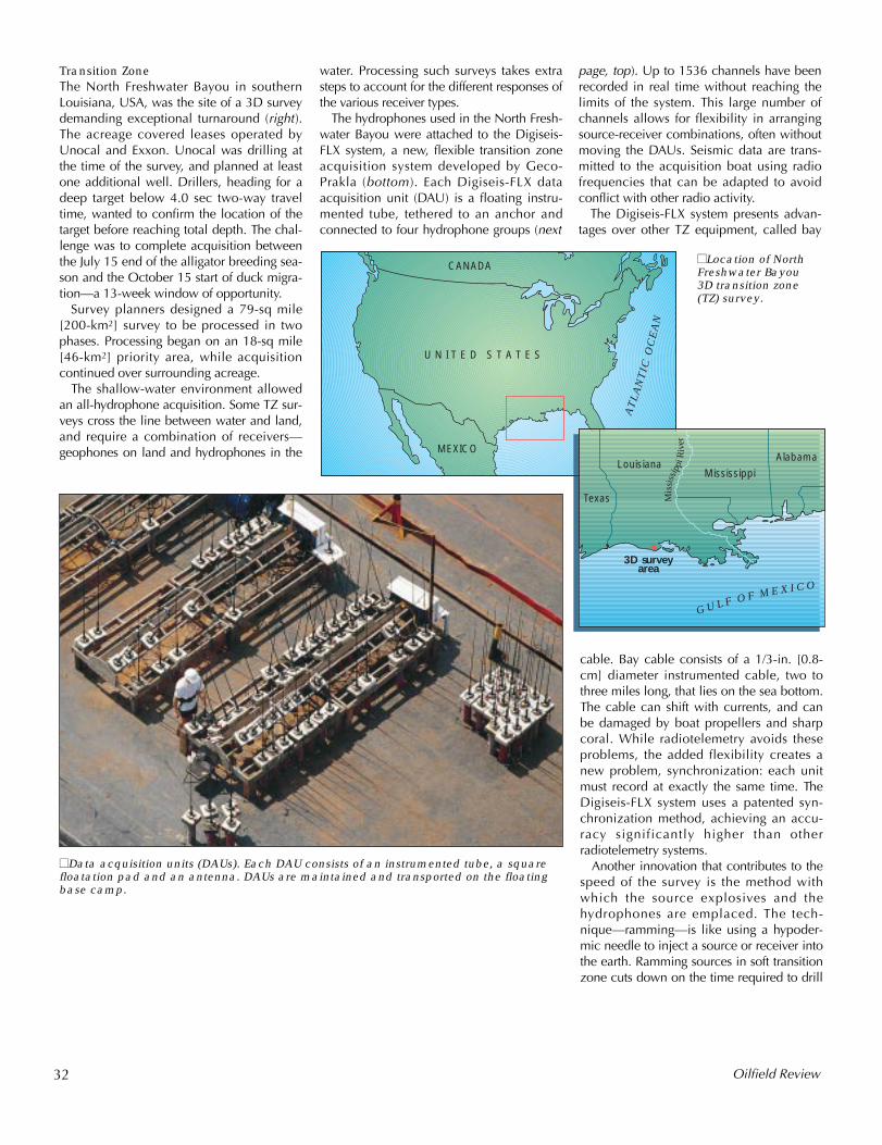
U N I T E D S T A T E S
CANADA
MEXICO
AT
LA
NT
ICO
CE
AN
Mis
siss
ippi
Riv
er
Mississippi
AlabamaLouisiana
Texas
G U L F O F M E X I C O
3D surveyarea
cable. Bay cable consists of a 1/3-in. [0.8-cm] diameter instrumented cable, two tothree miles long, that lies on the sea bottom.The cable can shift with currents, and canbe damaged by boat propellers and sharpcoral. While radiotelemetry avoids theseproblems, the added flexibility creates anew problem, synchronization: each unitmust record at exactly the same time. TheDigiseis-FLX system uses a patented syn-chronization method, achieving an accu-racy significantly higher than otherradiotelemetry systems.
Another innovation that contributes to thespeed of the survey is the method withwhich the source explosives and thehydrophones are emplaced. The tech-nique—ramming—is like using a hypoder-mic needle to inject a source or receiver intothe earth. Ramming sources in soft transitionzone cuts down on the time required to drill
Transition ZoneThe North Freshwater Bayou in southernLouisiana, USA, was the site of a 3D surveydemanding exceptional turnaround (right).The acreage covered leases operated byUnocal and Exxon. Unocal was drilling atthe time of the survey, and planned at leastone additional well. Drillers, heading for adeep target below 4.0 sec two-way traveltime, wanted to confirm the location of thetarget before reaching total depth. The chal-lenge was to complete acquisition betweenthe July 15 end of the alligator breeding sea-son and the October 15 start of duck migra-tion—a 13-week window of opportunity.
Survey planners designed a 79-sq mile[200-km2] survey to be processed in twophases. Processing began on an 18-sq mile[46-km2] priority area, while acquisitioncontinued over surrounding acreage.
The shallow-water environment allowedan all-hydrophone acquisition. Some TZ sur-veys cross the line between water and land,and require a combination of receivers—geophones on land and hydrophones in the
water. Processing such surveys takes extrasteps to account for the different responses ofthe various receiver types.
The hydrophones used in the North Fresh-water Bayou were attached to the Digiseis-FLX system, a new, flexible transition zoneacquisition system developed by Geco-Prakla (bottom). Each Digiseis-FLX dataacquisition unit (DAU) is a floating instru-mented tube, tethered to an anchor andconnected to four hydrophone groups (next
page, top). Up to 1536 channels have beenrecorded in real time without reaching thelimits of the system. This large number ofchannels allows for flexibility in arrangingsource-receiver combinations, often withoutmoving the DAUs. Seismic data are trans-mitted to the acquisition boat using radiofrequencies that can be adapted to avoidconflict with other radio activity.
The Digiseis-FLX system presents advan-tages over other TZ equipment, called bay
32 Oilfield Review
■■Location of NorthFreshwater Bayou3D transition zone(TZ) survey.
■■Data acquisition units (DAUs). Each DAU consists of an instrumented tube, a squarefloatation pad and an antenna. DAUs are maintained and transported on the floatingbase camp.
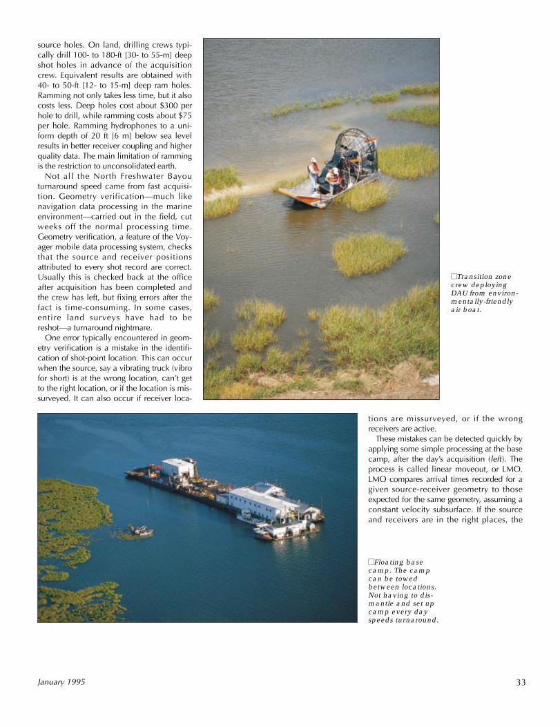
source holes. On land, drilling crews typi-cally drill 100- to 180-ft [30- to 55-m] deepshot holes in advance of the acquisitioncrew. Equivalent results are obtained with40- to 50-ft [12- to 15-m] deep ram holes.Ramming not only takes less time, but it alsocosts less. Deep holes cost about $300 perhole to drill, while ramming costs about $75per hole. Ramming hydrophones to a uni-form depth of 20 ft [6 m] below sea levelresults in better receiver coupling and higherquality data. The main limitation of rammingis the restriction to unconsolidated earth.
Not all the North Freshwater Bayouturnaround speed came from fast acquisi-tion. Geometry verification—much likenavigation data processing in the marineenvironment—carried out in the field, cutweeks off the normal processing time.Geometry verification, a feature of the Voy-ager mobile data processing system, checksthat the source and receiver positionsattributed to every shot record are correct.Usually this is checked back at the officeafter acquisition has been completed andthe crew has left, but fixing errors after thefact is time-consuming. In some cases,entire land surveys have had to bereshot—a turnaround nightmare.
One error typically encountered in geom-etry verification is a mistake in the identifi-cation of shot-point location. This can occurwhen the source, say a vibrating truck (vibrofor short) is at the wrong location, can’t getto the right location, or if the location is mis-surveyed. It can also occur if receiver loca-
33January 1995
■■Transition zonecrew deployingDAU from environ-mentally-friendlyair boat.
■■Floating basecamp. The campcan be towedbetween locations.Not having to dis-mantle and set upcamp every dayspeeds turnaround.
tions are missurveyed, or if the wrongreceivers are active.
These mistakes can be detected quickly byapplying some simple processing at the basecamp, after the day’s acquisition (left). Theprocess is called linear moveout, or LMO.LMO compares arrival times recorded for agiven source-receiver geometry to thoseexpected for the same geometry, assuming aconstant velocity subsurface. If the sourceand receivers are in the right places, the
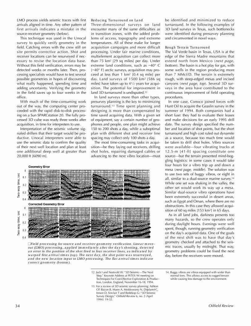
LMO process yields seismic traces with firstarrivals aligned in time. Any other pattern offirst arrivals indicates a mistake in thesource-receiver geometry (below).
This technique was used in the Unocalsurvey to quickly verify geometry in thefield. Catching errors with the crew still onsite permits corrective action. Shot andreceiver locations can be resurveyed if nec-essary to revise the location data base.Without this field verification, errors may bedetected weeks or months later. Then, pro-cessing specialists would have to test severalpossible geometries in hopes of discoveringwhat really happened, spending time andadding uncertainty. Verifying the geometryin the field saves up to four weeks in theoffice.
With much of the time-consuming workout of the way, the computing center pro-ceeded with the rapid disk-to-disk process-ing on a Sun SPARCstation 20. The fully pro-cessed 3D cube was ready three weeks afteracquisition, in time for interpreters to use.
Interpretation of the seismic volume sig-naled drillers that their target would be pro-ductive. Unocal interpreters were able touse the seismic data to confirm the qualityof their next well location and plan at leastone additional deep well at greater than20,000 ft [6090 m].
Reducing Turnaround on LandThree-dimensional surveys on landencounter many of the same difficulties asin transition zones, with the added prob-lems of access, topography and extremetemperatures. All of these make for longeracquisition campaigns and more difficultprocessing. Under fair marine conditions,multielement acquisition can collect morethan 75 km2 [29 sq miles] per day. Underextreme land conditions, such as −40° C[−40° F] arctic surveys, acquisition may pro-ceed at less than 1 km2 [0.4 sq mile] perday. Land surveys of 1500 km2 [586 sqmiles] have taken up to 41/2 years for acqui-sition. The potential for improvement inland 3D turnaround is undisputed.12
In land surveys more than other types,presurvey planning is the key to minimizingturnaround.13 Time spent planning anddesigning is more than compensated bytime saved acquiring data. With a given setof equipment, say a certain number of geo-phones and people, one plan might achieve150 to 200 shots a day, while a suboptimalplan with different shot and receiver linespacing may collect only 100 shots a day.
The most time-consuming tasks in acqui-sition—be they laying out receivers, drillingshot holes, repairing damaged cables oradvancing to the next vibro location—must
be identified and minimized to reduceturnaround. In the following examples of3D land surveys in Texas, such bottleneckswere identified during presurvey planningand circumvented in novel ways.
Rough Terrain TurnaroundThe Val Verde basin in Texas, USA is at theedge of the Sierra Madre mountains thatextend north from Mexico (next page,bottom). The basin is a hot play for gas, withsome wells in the region producing morethan 7 MMcf/D. The terrain is extremelyrough, with steep-edged mesas and incisedcanyons (next page, top). Several 3D sur-veys in the area have contributed to thecontinuous improvement of field operatingprocedures.
In one case, Conoco joined forces withHunt Oil to acquire the Geaslin survey in thesummer of 1994. Both companies had ashort fuse: they had to evaluate their leasesand make decisions for an early 1995 drilldate. The survey design specified the num-ber and location of shot points, but the shortturnaround and high cost ruled out dynamiteas a source, because too much time wouldbe taken to drill shot holes. Vibro sourceswere available—four vibrating trucks at12.5-m [41-ft] spacing constitute onesource—but the terrain presented mind-bog-gling logistics: in some cases it would takefour hours for a vibro trip up and down amesa (next page, middle). The solution wasto use two sets of buggy vibros, or eight inall, similar to a dual-source marine survey.14
While one set was shaking in the valley, theother set would work its way up a mesa.Similar dual-source vibro operations havebeen extremely successful in desert areas,such as Egypt and Oman, where there are noobstructions. In this case they allowed acqui-sition of 60 sq miles [153 km2] in 65 days.
As in all land jobs, darkness presents toomany hazards, so the crew operates onlyduring daylight hours. Evenings were wellspent, though, running geometry verificationon the day’s acquired data. One of the goalsof the next shift was to have that day’sgeometry checked and attached to the seis-mic traces, usually by midnight. That way,geometry problems could be fixed the nextday, before the receivers were moved.
34 Oilfield Review
■■Field processing for source and receiver geometry verification. Linear move-out (LMO) processing, applied immediately after the day’s shooting, detectedan error in the position of the shot fired to four receiver lines, as indicated bywarped first arrival times (top). The next day, the shot point was resurveyed,and the new location input to LMO processing. The flat arrival times indicatecorrect geometry (bottom).
12. Jack I and Nestvold W: “3D Seismic—The NextStep,” Keynote Address at PETEX 94 meeting onTechniques For Cost-Effective Exploration & Produc-tion, London, England, November 16-18, 1994.
13. For a review of 3D seismic survey planning: AshtonCP, Bacon B, Mann A, Moldoveanu N, Déplanté C,Ireson D, Sinclair T and Redekop G: “3D SeismicSurvey Design,” Oilfield Review 6, no. 2 (April1994): 19-32.
0
0.1
0.2
0.3
0.4
0
0.1
0.2
0.3
0.4
Two-
way
tim
e, s
ecTw
o-w
ay ti
me,
sec
Geometry Error
Corrected Geometry Error
14. Buggy vibros are vibros equipped with wider thannormal tires. This allows access to rugged terrainwhile causing less damage to the environment.
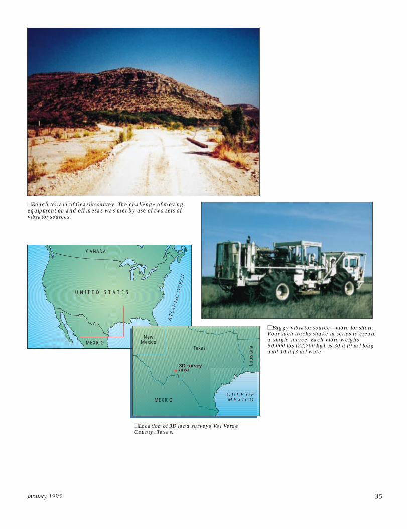
U N I T E D S T A T E S
CANADA
MEXICO
AT
LA
NT
ICO
CE
AN
Loui
sian
aTexas
G U L F O F M E X I C O
3D surveyarea
MEXICO
NewMexico
■■Buggy vibrator source—vibro for short.Four such trucks shake in series to createa single source. Each vibro weighs50,000 lbs [22,700 kg], is 30 ft [9 m] longand 10 ft [3 m] wide.
35January 1995
■■Location of 3D land surveys Val VerdeCounty, Texas.
■■Rough terrain of Geaslin survey. The challenge of movingequipment on and off mesas was met by use of two sets ofvibrator sources.
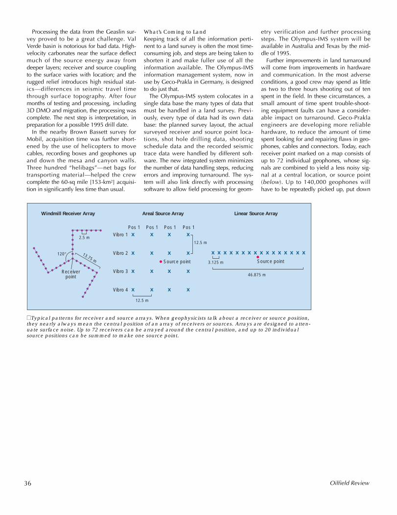
What’s Coming to LandKeeping track of all the information perti-nent to a land survey is often the most time-consuming job, and steps are being taken toshorten it and make fuller use of all theinformation available. The Olympus-IMSinformation management system, now inuse by Geco-Prakla in Germany, is designedto do just that.
The Olympus-IMS system colocates in asingle data base the many types of data thatmust be handled in a land survey. Previ-ously, every type of data had its own database: the planned survey layout, the actualsurveyed receiver and source point loca-tions, shot hole drilling data, shootingschedule data and the recorded seismictrace data were handled by different soft-ware. The new integrated system minimizesthe number of data handling steps, reducingerrors and improving turnaround. The sys-tem will also link directly with processingsoftware to allow field processing for geom-
Processing the data from the Geaslin sur-vey proved to be a great challenge. ValVerde basin is notorious for bad data. High-velocity carbonates near the surface deflectmuch of the source energy away fromdeeper layers; receiver and source couplingto the surface varies with location; and therugged relief introduces high residual stat-ics—differences in seismic travel timethrough surface topography. After fourmonths of testing and processing, including3D DMO and migration, the processing wascomplete. The next step is interpretation, inpreparation for a possible 1995 drill date.
In the nearby Brown Bassett survey forMobil, acquisition time was further short-ened by the use of helicopters to movecables, recording boxes and geophones upand down the mesa and canyon walls.Three hundred “helibags”—net bags fortransporting material—helped the crewcomplete the 60-sq mile [153-km2] acquisi-tion in significantly less time than usual.
etry verification and further processingsteps. The Olympus-IMS system will beavailable in Australia and Texas by the mid-dle of 1995.
Further improvements in land turnaroundwill come from improvements in hardwareand communication. In the most adverseconditions, a good crew may spend as littleas two to three hours shooting out of tenspent in the field. In these circumstances, asmall amount of time spent trouble-shoot-ing equipment faults can have a consider-able impact on turnaround. Geco-Praklaengineers are developing more reliablehardware, to reduce the amount of timespent looking for and repairing flaws in geo-phones, cables and connectors. Today, eachreceiver point marked on a map consists ofup to 72 individual geophones, whose sig-nals are combined to yield a less noisy sig-nal at a central location, or source point(below). Up to 140,000 geophones willhave to be repeatedly picked up, put down
36 Oilfield Review
■■Typical patterns for receiver and source arrays. When geophysicists talk about a receiver or source position,they nearly always mean the central position of an array of receivers or sources. Arrays are designed to atten-uate surface noise. Up to 72 receivers can be arrayed around the central position, and up to 20 individualsource positions can be summed to make one source point.
Areal Source Array
12.5 m
x
x
x x
x x x
x x
x x
x
12.5 m
Source point
Vibro 1
Pos 1 Pos 1 Pos 1 Pos 1
Vibro 2
Vibro 3
Vibro 4
x
x
x
x
Linear Source Array
x x x x x x x x x x x x x x x x
3.125 m Source point
46.875 m
Windmill Receiver Array
2.5 m
13.75 m120°
Receiverpoint
and maintained in the course of a 3D sur-vey. Efforts are also underway to find newways to acquire the same amount and qual-ity of data with fewer receivers, cutting sur-vey time.
Improved communications will also cutturnaround time. Increased use of GPS isdecreasing the time spent surveying posi-tions for land source and receiver points.Surveying with GPS is faster and easier tocheck than traditional theodolitic surveying,and leaves less room for human error. Plac-ing GPS units on vibro sources helps keeptrack of actual source locations and reduceslocation error.
For arctic land surveys, snow streamershave been developed in collaboration withNorsk Hydro as substitutes for hand-placedgeophones in an effort to increase acquisi-tion efficiency. Geco-Prakla engineers havetested snow streamers in six programs,acquiring 1200 km [750 miles] of 2D data.Efforts are also underway to minimize envi-ronmental impact, which in arctic environ-ments must be included as part ofturnaround—a single drop of oil spilledmust be recovered before the crew moves.15
Connecting land crews via satellite toSINet, the Schlumberger Information Net-work, will give better day-to-day contactwith office bases, speeding equipment andsupply requests and allowing interactionwith processing centers. The first such satel-lite link has been made in Venezuela, andothers are planned.
Moving more processing to the field willfurther reduce turnaround for both land andtransition zone surveys. Parameter testing,noise attenuation and velocity picking canbe done with today’s field processing tools.But full concurrent processing, as performedin marine surveys, is still a dream for land.Land acquisition, more so than marine, is athree-dimensional problem: sources are notaligned with receiver lines, and more time isneeded to acquire enough seismic traces toprocess one part of the 3D volume. At best,processing through to stacking could lagacquisition by a few weeks, but the difficulttask of computing residual statics beforestacking cannot begin until all the data arein. Advances may come from taking a newview of 3D land surveys—planning, acquir-ing and processing with a truly three-dimen-sional view—rather than simply repeating aseries of two-dimensional snapshots.
The Role of Integrated Services in Reducing TurnaroundMarine, TZ and land 3D surveys are sure tofind further turnaround improvement in thecommon ground of integrated services. In anintegrated-service survey, planning, acquisi-tion, processing and project managementare delivered by one service company. Tradi-tionally, the oil company plans the survey,then one contractor acquires the data andanother processes it. Time is wasted transfer-ring data and responsibility between parties.
Geco-Prakla has developed an integratedservice for 3D surveys called TQ3D—TotalQuality 3D. Larger in area than most sur-veys, TQ3D projects can cover leased andopen blocks. A TQ3D project may be oper-ated from 100% proprietary to 100% nonex-clusive, or anywhere in between. Dataacquired on a proprietary basis become theproperty of the operator. Large projects caninvolve several operators. Data acquired ona nonexclusive basis become the property ofGeco-Prakla, and may be licensed.
The turnaround improvement achievablethrough integrated services is remarkable. Amixed proprietary-nonexclusive TQ3D forBP in UK block 47/10 was started and com-pleted in November 1994. Geco Topazacquired the 230-km2 [89-sq mile] survey inthree weeks. While full-fold data were beingacquired, a 20-fold data volume was par-tially migrated onboard, and processing wascompleted onshore. Processed data weresent to the GeoQuest Data Services groupvia SINet, and converted to Charisma work-station format. Total project time was fourweeks. Thirty-four such marine surveys havebeen completed, and 21 more are inprogress, covering a total of 43,000 km2
[16,800 sq miles].Integrated services are also reducing land
survey turnaround. Land surveys, with theirdifficult logistics, benefit from the approacha committed team brings to a project. Inaddition to survey design, acquisition andprocessing, land surveys require obtainingpermission to access an area from thosewho own and live on the land. The projectcan run more smoothly when a single con-tractor coordinates every phase. One suchproject in Africa turned around a 50-km2
[20-sq mile] survey in seven months, fromplanning through installation of processeddata onto an interpretation workstation. Twoother projects are in the survey design stage.
January 1995
15. For more on arctic surveys: Meyer H, Read T,Thomas J, Wedge M and Wren M: “EnvironmentalManagement in the Arctic,” Oilfield Review 5, no. 4(October 1993): 14-22.
For marine, transition zone and land 3Dsurvey turnaround, the journey is not fin-ished, but the direction is clear. Marine sur-veys are in the lead, having made tremen-dous progress in the last three years byconverting acquisition, positioning and pro-cessing to a set of parallel tasks. Somemarine surveys that would have taken 10years to acquire and process using 1980stechnology are now completed in months.Some say marine turnaround is no longer anissue, that any marine survey can now beturned around within any explorationist‘stime constraint.
Land and transition zone surveys, whilelagging their marine counterparts, havemade inroads with field processing, innova-tive sources and survey designs that opti-mize available equipment. These and furtherimprovements will contribute to minimizingturnaround time, allowing oil companies tospend less time waiting for information andmore time using it. —LS
37
38
lution in our ability to evalu-
munity of interpreters
g carbonate reservoirs to
Classic Interpretation Problems: Evaluating Carbonates
Mahmood AkbarMario PetricolaMohamed WatfaAbu Dhabi, United Arab Emirates
Mohammed BadriMouhab ChararaCairo, Egypt
Austin BoydDenver, Colorado, USA
Bruce CassellRoy NurmiDubai, United Arab Emirates
Jean-Pierre DelhommeClamart, France
Mike GraceDallas, Texas, USA
Bill KenyonRidgefield, Connecticut, USA
Jon RoestenburgJakarta, Indonesia
ian Singer, Schlumberger Wireline & Testing,i, India; and Eric Standen, Schlumberger Wire-ing, Montrouge, France.le, ARI (Azimuthal Resistivity Imager), CMRle Magnetic Resonance tool), DSI (Dipolec Imager), EPT (Electromagnetic Propagation(Fullbore Formation MicroImager), FracView,, MDT (Modular Formation Dynamics Tester)hermal Decay Time) are marks of Schlum-
r behavior. This article tracks theation process, from carbonate rockon and petrophysical log evaluationechniques for measuring permeabil-hole and mapping large-scale flow and barriers.
ates for Beginnerstes and sand-shale rocks, or silici-are worlds apart. Whereas siliciclas- are composed of a variety of silica-grains that may have traveleds of miles from their source, carbon-s mainly consist of just two miner-ite and dolomite—and remain nearint of origin.1 Carbonates form inand deep marine settings, evaporiticakes and windy deserts.2 Most of thetes formed in past have shallow
INTERPRETATION
In recent years, there has been a small revo
ate carbonates. Novel technology and a com
determined to crack one hard nut are forcin
reveal many of their secrets.
For help in preparation of this article, thanks to HervéAnxionnaz, Schlumberger Wireline & Testing, Clamart,France; Jean-Louis Chardac, Schlumberger Wireline &Testing, Dubai, UAE; Bob Dennis, Schlumberger Wire-line & Testing, Wattayh, Oman; Philip Cheung, ArnaudEtchecopar and Ollivier Faivre, Schlumberger Wireline &Testing, Clamart, France; Brian Hornby, SchlumbergerCambridge Research, Cambridge, England; Rachel Korn-berg, GeoQuest, Gatwick, England; William Murphy andPabitra Sen, Schlumberger-Doll Research, Ridgefield,Connecticut, USA; Oberto Serra, Consultant, Paris,
France; JulNew Delhline & TestIn this artic(CombinabShear SoniTool), FMI GeoFrameand TDT (Tberger.
Carbonate reservoirs account for 40% oftoday’s hydrocarbon production, andbecause of several elephant fields in theMiddle East they are expected to dominateproduction through the next century. There-fore, understanding carbonate reservoirsand producing them efficiently havebecome industry priorities and are likely toremain so.
Current efforts in carbonate exploitationfocus on correctly targeting new wells, fre-quently horizontal, to optimize productionfrom untouched reserves and on ensuringthat massive water injection schemes deliveran effective sweep of the reservoir. In sup-port of these efforts, geoscientists are tryingto decipher the enigma of carbonate rock’scomplex pore space and understand howpermeability barriers and conduits affect
reservoiinterpretdescriptito new tity downconduits
CarbonCarbonaclastics, tic rocksbased hundredate rockals—calctheir poshallow basins, lcarbona
Oilfield Review
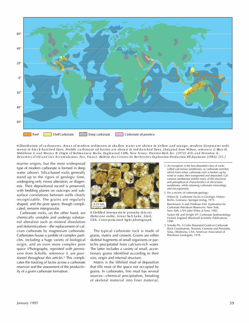
39January 1995
nDistribution of carbonates. Areas of modern sediments in shallow water are shown in yellow and orange, modern deepwater sedi-ments in black-hatched lines. Prolific carbonate oil basins are shown in red-hatched lines. [Adapted from Wilson, reference 2; Blatt H,Middleton G and Murray R: Origin of Sedimentary Rocks. Englewood Cliffs, New Jersey: Prentice-Hall, Inc. (1972): 410; and Perrodon A:Dynamics of Oil and Gas Accumulations. Pau, France: Bulletin des Centres de Recherches Exploration-Production Elf-Aquitaine (1983): 215.]
nUnfilled interparticle porosity (black).Holocene oolite, Great Salt Lake, Utah,USA. Cross-polarized light photograph.
1. An exception is the less-abundant class of rocks called calcareous sandstones, or carbonate arenites,which form when carbonate rock is broken up bywind or water, then transported and deposited. Cal-careous sandstones exhibit many of the structural and petrophysical characteristics of siliciclastic sandstones, while retaining carbonate mineralogy and microporosity.
2. For a review of carbonate geology:Wilson JL: Carbonate Facies in Geologic History.Berlin, Germany: Springer-Verlag, 1975.Reeckmann A and Friedman GM: Exploration for Carbonate Petroleum Reservoirs. New York, New York, USA: John Wiley & Sons, 1982.Tucker ME and Wright VP: Carbonate Sedimentology.Oxford, England: Blackwell Scientific Publications,1990.
3. Scholle PA: A Color Illustrated Guide to CarbonateRock Constitutents, Textures, Cements and Porosities.Tulsa, Oklahoma, USA: American Association ofPetroleum Geologists, 1978.
marine origins, but the most widespreadtype of modern carbonate is formed in deepwater (above). Silica-based rocks generallystand up to the rigors of geologic time,undergoing only minor alteration, or diagen-esis. Their depositional record is preserved,with bedding planes on outcrops and sub-surface correlations between wells clearlyrecognizable. The grains are regularlyshaped, and the pore space, though compli-cated, remains intergranular.
Carbonate rocks, on the other hand, arechemically unstable and undergo substan-tial alteration such as mineral dissolutionand dolomitization—the replacement of cal-cium carbonate by magnesium carbonate.Carbonates house a jumble of complex parti-cles, including a huge variety of biologicalorigin, and an even more complex porespace (Photographs, reprinted with permis-sion from Scholle, reference 3, are posi-tioned throughout this article).3 This compli-cates the tracking of facies across a carbonatereservoir and the assessment of the productiv-ity of a given carbonate formation.
The typical carbonate rock is made ofgrains, matrix and cement. Grains are eitherskeletal fragments of small organisms or par-ticles precipitated from calcium-rich water.The latter includes a variety of small, accre-tionary grains identified according to theirsize, origin and internal structure.
Matrix is the lithified mud of depositionthat fills most of the space not occupied bygrains. In carbonates, fine mud has severalsources—chemical precipitation, breakingof skeletal material into finer material,
40°
60°
20°
0°
20°
40°
60°
Reef Shelf carbonate Deep carbonate Carbonate oil province
0.23 mm
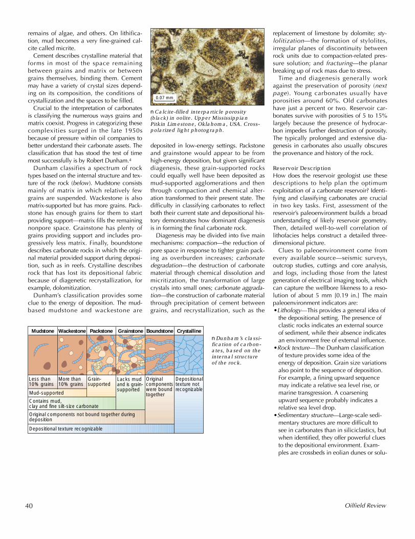
replacement of limestone by dolomite; sty-lolitization—the formation of stylolites,irregular planes of discontinuity betweenrock units due to compaction-related pres-sure solution; and fracturing—the planarbreaking up of rock mass due to stress.
Time and diagenesis generally workagainst the preservation of porosity (nextpage). Young carbonates usually haveporosities around 60%. Old carbonateshave just a percent or two. Reservoir car-bonates survive with porosities of 5 to 15%largely because the presence of hydrocar-bon impedes further destruction of porosity.The typically prolonged and extensive dia-genesis in carbonates also usually obscuresthe provenance and history of the rock.
Reservoir DescriptionHow does the reservoir geologist use thesedescriptions to help plan the optimumexploitation of a carbonate reservoir? Identi-fying and classifying carbonates are crucialin two key tasks. First, assessment of thereservoir’s paleoenvironment builds a broadunderstanding of likely reservoir geometry.Then, detailed well-to-well correlation oflithofacies helps construct a detailed three-dimensional picture.
Clues to paleoenvironment come fromevery available source—seismic surveys,outcrop studies, cuttings and core analysis,and logs, including those from the latestgeneration of electrical imaging tools, whichcan capture the wellbore likeness to a reso-lution of about 5 mm [0.19 in.] The mainpaleoenvironment indicators are:•Lithology—This provides a general idea of
the depositional setting. The presence ofclastic rocks indicates an external sourceof sediment, while their absence indicatesan environment free of external influence.
•Rock texture—The Dunham classificationof texture provides some idea of theenergy of deposition. Grain size variationsalso point to the sequence of deposition.For example, a fining upward sequencemay indicate a relative sea level rise, ormarine transgression. A coarseningupward sequence probably indicates arelative sea level drop.
•Sedimentary structure—Large-scale sedi-mentary structures are more difficult tosee in carbonates than in siliciclastics, butwhen identified, they offer powerful cluesto the depositional environment. Exam-ples are crossbeds in eolian dunes or solu-
remains of algae, and others. On lithifica-tion, mud becomes a very fine-grained cal-cite called micrite.
Cement describes crystalline material thatforms in most of the space remainingbetween grains and matrix or betweengrains themselves, binding them. Cementmay have a variety of crystal sizes depend-ing on its composition, the conditions ofcrystallization and the spaces to be filled.
Crucial to the interpretation of carbonatesis classifying the numerous ways grains andmatrix coexist. Progress in categorizing thesecomplexities surged in the late 1950sbecause of pressure within oil companies tobetter understand their carbonate assets. Theclassification that has stood the test of timemost successfully is by Robert Dunham.4
Dunham classifies a spectrum of rocktypes based on the internal structure and tex-ture of the rock (below). Mudstone consistsmainly of matrix in which relatively fewgrains are suspended. Wackestone is alsomatrix-supported but has more grains. Pack-stone has enough grains for them to startproviding support—matrix fills the remainingnonpore space. Grainstone has plenty ofgrains providing support and includes pro-gressively less matrix. Finally, boundstonedescribes carbonate rocks in which the origi-nal material provided support during deposi-tion, such as in reefs. Crystalline describesrock that has lost its depositional fabricbecause of diagenetic recrystallization, forexample, dolomitization.
Dunham’s classification provides someclue to the energy of deposition. The mud-based mudstone and wackestone are
40 Oilfield Review
deposited in low-energy settings. Packstoneand grainstone would appear to be fromhigh-energy deposition, but given significantdiagenesis, these grain-supported rockscould equally well have been deposited asmud-supported agglomerations and thenthrough compaction and chemical alter-ation transformed to their present state. Thedifficulty in classifying carbonates to reflectboth their current state and depositional his-tory demonstrates how dominant diagenesisis in forming the final carbonate rock.
Diagenesis may be divided into five mainmechanisms: compaction—the reduction ofpore space in response to tighter grain pack-ing as overburden increases; carbonatedegradation—the destruction of carbonatematerial through chemical dissolution andmicritization, the transformation of largecrystals into small ones; carbonate aggrada-tion—the construction of carbonate materialthrough precipitation of cement betweengrains, and recrystallization, such as the
Mudstone Wackestone Packstone Grainstone Boundstone Crystalline
Less than10% grains
More than10% grains
Mud-supported
Contains mud,clay and fine silt-size carbonate
Original components not bound together duringdeposition
Depositional texture recognizable
Grain-supported
Lacks mudand is grain-supported
Originalcomponentswere boundtogether
Depositionaltexture notrecognizable
nDunham’s classi-fication of carbon-ates, based on theinternal structureof the rock.
nCalcite-filled interparticle porosity(black) in oolite. Upper MississippianPitkin Limestone, Oklahoma, USA. Cross-polarized light photograph.
0.07 mm
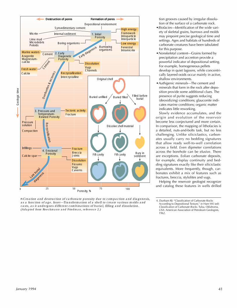
tion grooves caused by irregular dissolu-tion of the surface of a carbonate rock.
•Biofacies—Identification of the wide vari-ety of skeletal grains, burrows and moldsmay pinpoint precise geological time andsettings. Ages and habitats of hundreds ofcarbonate creatures have been tabulatedfor this purpose.
•Nonskeletal content—Grains formed byprecipitation and accretion provide apowerful indicator of depositional setting.For example, homogeneous pelletsdevelop in quiet lagoons, while concentri-cally layered ooids occur mainly in active,shallow environments.
•Authigenic minerals—The cement andminerals that form in the rock after depo-sition provide some additional clues. Thepresence of pyrite suggests reducing(deoxidizing) conditions; glauconite indi-cates marine conditions; organic matterindicates little reworking.Slowly evidence accumulates, and the
origin and evolution of the reservoirbecome less conjectured and more certain.In comparison, the mapping of lithofacies isa detailed, nuts-and-bolts task, but no lesschallenging. Unlike siliciclastics, carbon-ates usually carry no bedding signaturesthat allow ready well-to-well correlationacross a field. Even dipmeter correlationsacross the borehole can be elusive. Thereare exceptions. Eolian carbonate deposits,for example, display continuity and bed-ding signatures exactly like their siliciclasticequivalents. More frequently, though, car-bonates exhibit a mix of features such asfractures, breccia, stylolites and vugs.
Helping the reservoir geologist recognizeand catalog these features in wells drilled
41January 1994
nCreation and destruction of carbonate porosity due to compaction and diagenesis,as a function of age. Inset—Transformation of a shell to create various molds andcasts, as it undergoes different combinations of burial, filling and dissolution.(Adapted from Reeckmann and Friedman, reference 2.)
4. Dunham RJ: “Classification of Carbonate RocksAccording to Depositional Texture,” in Ham WE (ed):Classification of Carbonate Rocks. Tulsa, Oklahoma,USA: American Association of Petroleum Geologists,1962.
DissolutionFissuresVugsCaverns
FractureBrecciaJoints
4. Erosional Porosity
Late
buria
l
diage
nesis
Calcite spar
Infillings
3. Pressure-and Temperature- Related Porosity
Pressuresolution
Compaction
Tectonic activityFracture
Calcite
Marine watersAragoniteMagnesium-calcite
Fresh water Cemen
t
Cement
RecrystallizationIntercrystalline
DissolutionVugsChannels
Burrowingorganisms
1. InitialPorosity
2. EarlyDiageneticPorosity
Low energyFenestralIntramicrite
High energyFrameworkIntraparticleInterparticle
Formation of pores
Depositional environmentSynsedimentary cement
Internal sediment
Boring organisms
Micrite
Lime mudMicrodebrisPeloids
Destruction of poresG
eolo
gic
time
Early diagenesis
50250 75 100Porosity, %
Original shell
Buried unfilled Buried filled Filled beforeburial
Dissolve shell material
Fill cavity Bury insedimentFill cavity
Recrystallization
Ove
rbur
den
&te
cton
ics
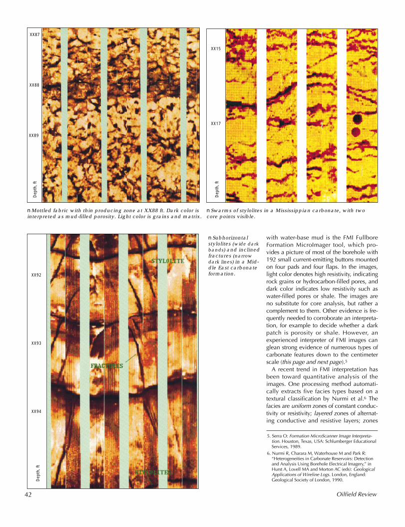
nSubhorizontal stylolites (wide darkbands) and inclinedfractures (narrowdark lines) in a Mid-dle East carbonateformation.
nMottled fabric with thin producing zone at XX88 ft. Dark color isinterpreted as mud-filled porosity. Light color is grains and matrix.
42 Oilfield Review
nSwarms of stylolites in a Mississippian carbonate, with twocore points visible.
XX93
XX92
XX94
Dep
th, f
t
XX88
XX87
XX89
Dep
th, f
t
Dep
th, f
t
XX15
XX17
with water-base mud is the FMI FullboreFormation MicroImager tool, which pro-vides a picture of most of the borehole with192 small current-emitting buttons mountedon four pads and four flaps. In the images,light color denotes high resistivity, indicatingrock grains or hydrocarbon-filled pores, anddark color indicates low resistivity such aswater-filled pores or shale. The images areno substitute for core analysis, but rather acomplement to them. Other evidence is fre-quently needed to corroborate an interpreta-tion, for example to decide whether a darkpatch is porosity or shale. However, anexperienced interpreter of FMI images canglean strong evidence of numerous types ofcarbonate features down to the centimeterscale (this page and next page).5
A recent trend in FMI interpretation hasbeen toward quantitative analysis of theimages. One processing method automati-cally extracts five facies types based on atextural classification by Nurmi et al.6 Thefacies are uniform zones of constant conduc-tivity or resistivity; layered zones of alternat-ing conductive and resistive layers; zones
5. Serra O: Formation MicroScanner Image Interpreta-tion. Houston, Texas, USA: Schlumberger EducationalServices, 1989.
6. Nurmi R, Charara M, Waterhouse M and Park R:“Heterogeneities in Carbonate Reservoirs: Detectionand Analysis Using Borehole Electrical Imagery,” inHurst A, Lovell MA and Morton AC (eds): GeologicalApplications of Wireline Logs. London, England: Geological Society of London, 1990.
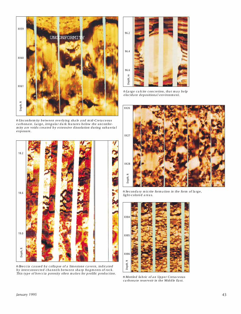
nSecondary micrite formation in the form of large,light-colored areas.
XX27
XX26
XX28
Dep
th, f
t
43January 1995
nUnconformity between overlying shale and mid-Cretaceouscarbonate. Large, irregular dark features below the unconfor-mity are voids created by extensive dissolution during subaerialexposure.
nBreccia caused by collapse of a limestone cavern, indicatedby interconnected channels between sharp fragments of rock.This type of breccia porosity often makes for prolific production.
nLarge calcite concretion, that may helpelucidate depositional environment.
nMottled fabric of an Upper Cretaceouscarbonate reservoir in the Middle East.
Dep
th, m
96.2
96.4
96.6
Dep
th, f
t
XX84
XX85
XX86
XX60
XX59
XX61
Dep
th, f
t
19.0
18.2
18.6
Dep
th, f
t
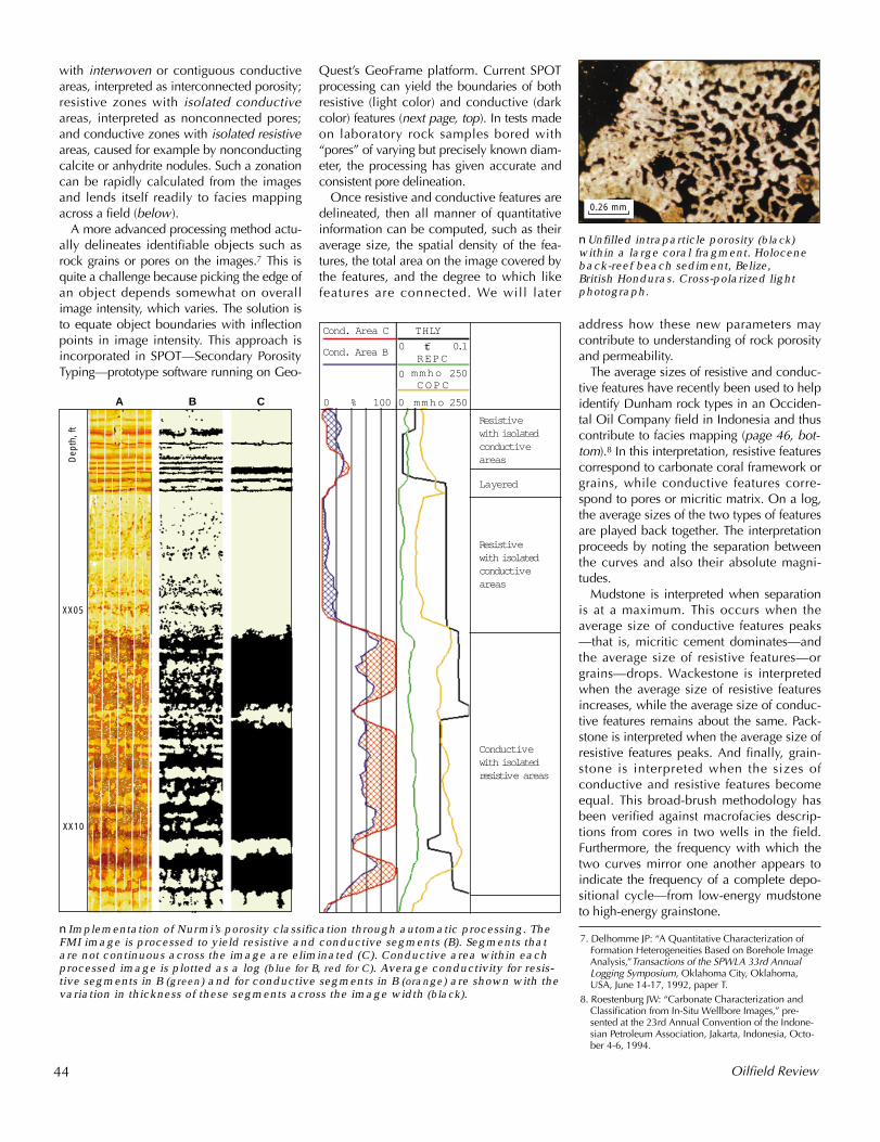
Dep
th, f
t
XX05
XX10
Layered
Resistive with isolatedconductiveareas
Resistive with isolatedconductiveareas
Conductive with isolatedresistive areas
Cond. Area C
Cond. Area B
THLY
REPC
C O P Cmmho
mmho
0
0
0
0.1
0 100
250
250
ft
%A B C
with interwoven or contiguous conductiveareas, interpreted as interconnected porosity;resistive zones with isolated conductiveareas, interpreted as nonconnected pores;and conductive zones with isolated resistiveareas, caused for example by nonconductingcalcite or anhydrite nodules. Such a zonationcan be rapidly calculated from the imagesand lends itself readily to facies mappingacross a field (below).
A more advanced processing method actu-ally delineates identifiable objects such asrock grains or pores on the images.7 This isquite a challenge because picking the edge ofan object depends somewhat on overallimage intensity, which varies. The solution isto equate object boundaries with inflectionpoints in image intensity. This approach isincorporated in SPOT—Secondary PorosityTyping—prototype software running on Geo-
Quest’s GeoFrame platform. Current SPOTprocessing can yield the boundaries of bothresistive (light color) and conductive (darkcolor) features (next page, top). In tests madeon laboratory rock samples bored with“pores” of varying but precisely known diam-eter, the processing has given accurate andconsistent pore delineation.
Once resistive and conductive features aredelineated, then all manner of quantitativeinformation can be computed, such as theiraverage size, the spatial density of the fea-tures, the total area on the image covered bythe features, and the degree to which likefeatures are connected. We will later
address how these new parameters maycontribute to understanding of rock porosityand permeability.
The average sizes of resistive and conduc-tive features have recently been used to helpidentify Dunham rock types in an Occiden-tal Oil Company field in Indonesia and thuscontribute to facies mapping (page 46, bot-tom).8 In this interpretation, resistive featurescorrespond to carbonate coral framework orgrains, while conductive features corre-spond to pores or micritic matrix. On a log,the average sizes of the two types of featuresare played back together. The interpretationproceeds by noting the separation betweenthe curves and also their absolute magni-tudes.
Mudstone is interpreted when separationis at a maximum. This occurs when theaverage size of conductive features peaks—that is, micritic cement dominates—andthe average size of resistive features—orgrains—drops. Wackestone is interpretedwhen the average size of resistive featuresincreases, while the average size of conduc-tive features remains about the same. Pack-stone is interpreted when the average size ofresistive features peaks. And finally, grain-stone is interpreted when the sizes ofconductive and resistive features becomeequal. This broad-brush methodology hasbeen verified against macrofacies descrip-tions from cores in two wells in the field.Furthermore, the frequency with which thetwo curves mirror one another appears toindicate the frequency of a complete depo-sitional cycle—from low-energy mudstoneto high-energy grainstone.
44 Oilfield Review
nImplementation of Nurmi’s porosity classification through automatic processing. TheFMI image is processed to yield resistive and conductive segments (B). Segments thatare not continuous across the image are eliminated (C). Conductive area within eachprocessed image is plotted as a log (blue for B, red for C). Average conductivity for resis-tive segments in B (green) and for conductive segments in B (orange) are shown with thevariation in thickness of these segments across the image width (black).
7. Delhomme JP: “A Quantitative Characterization ofFormation Heterogeneities Based on Borehole ImageAnalysis,”Transactions of the SPWLA 33rd AnnualLogging Symposium, Oklahoma City, Oklahoma,USA, June 14-17, 1992, paper T.
8. Roestenburg JW: “Carbonate Characterization andClassification from In-Situ Wellbore Images,” pre-sented at the 23rd Annual Convention of the Indone-sian Petroleum Association, Jakarta, Indonesia, Octo-ber 4-6, 1994.
nUnfilled intraparticle porosity (black)within a large coral fragment. Holoceneback-reef beach sediment, Belize,British Honduras. Cross-polarized lightphotograph.
0.26 mm
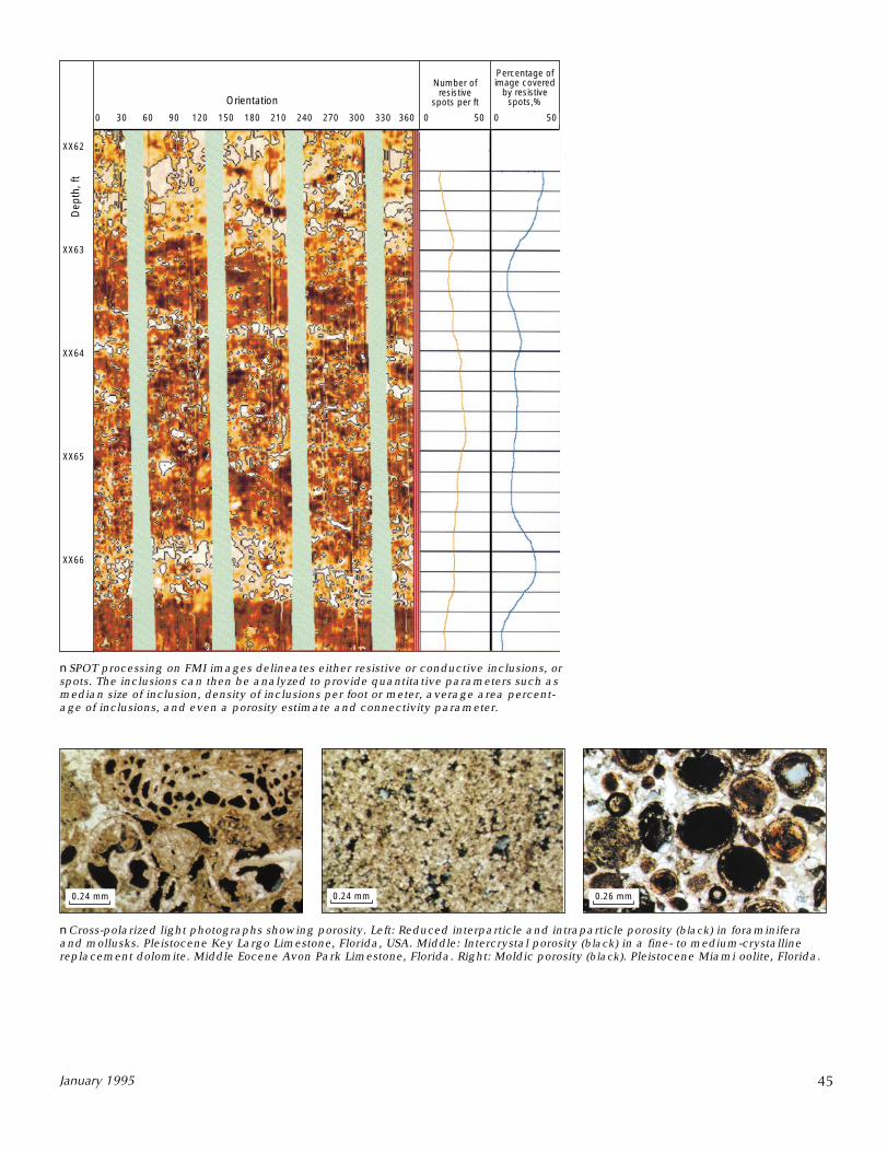
nCross-polarized light photographs showing porosity. Left: Reduced interparticle and intraparticle porosity (black) in foraminiferaand mollusks. Pleistocene Key Largo Limestone, Florida, USA. Middle: Intercrystal porosity (black) in a fine- to medium-crystallinereplacement dolomite. Middle Eocene Avon Park Limestone, Florida. Right: Moldic porosity (black). Pleistocene Miami oolite, Florida.
45January 1995
nSPOT processing on FMI images delineates either resistive or conductive inclusions, orspots. The inclusions can then be analyzed to provide quantitative parameters such asmedian size of inclusion, density of inclusions per foot or meter, average area percent-age of inclusions, and even a porosity estimate and connectivity parameter.
0.24 mm 0.24 mm 0.26 mm
XX62
0 30 60 90 120 150 180 210 240 270 300 330 360
XX63
XX64
XX65
XX66
Number ofresistive
spots per ft
Percentage ofimage covered
by resistivespots,%Orientation
0 050 50
Dep
th, f
t
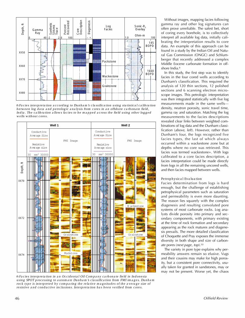
Without images, mapping facies followinggamma ray and other log signatures canoften prove unreliable. The safest bet, shortof coring every borehole, is to collectivelyinterpret all available log data, initially cali-brating the interpretation results to coredata. An example of this approach can befound in a study by the Indian Oil and Natu-ral Gas Commission (ONGC) and Schlum-berger that recently addressed a complexMiddle Eocene carbonate formation in off-shore India.9
In this study, the first step was to identifyfacies in the four cored wells according toDunham’s classification. This required theanalysis of 120 thin sections, 12 polishedsections and 6 scanning electron micro-scope images. This petrologic interpretationwas then integrated statistically with five logmeasurements made in the same wells—density, neutron porosity, sonic travel time,gamma ray and saturation. Matching the logmeasurements to the facies descriptionsrevealed clear links between weighted com-binations of log data and the Dunham classi-fication (above, left). However, rather thanDunham’s four, the logs recognized fivefacies types, the last of which alwaysoccurred within a wackestone zone but atdepths where no core was retrieved. Thisfacies was termed wackestone+. With logscalibrated to a core facies description, afacies interpretation could be made directlyfrom logs in all the remaining uncored wells,and then facies mapped between wells.
Petrophysical EvaluationFacies determination from logs is hardenough, but the challenge of establishingpetrophysical parameters such as saturationand permeability is even more daunting.The reason lies squarely with the complexdiagenesis and resulting convoluted poresystems of most carbonate rocks. Log ana-lysts divide porosity into primary and sec-ondary components, with primary existingat the time of rock formation and secondaryappearing as the rock matures and diagene-sis prevails. The more detailed classificationof Choquette and Pray exposes the immensediversity in both shape and size of carbon-ate pores (next page, top).10
The variety in pore type explains why per-meability answers remain so elusive. Vugsand their cousins may make for high poros-ity, but a consistent pore connectivity, usu-ally taken for granted in sandstones, may ormay not be present. Worse yet, the chaos
46 Oilfield Review
nFacies interpretation according to Dunham’s classification using statistical calibrationbetween log data and petrologic analysis from cores in an offshore carbonate field,India. The calibration allows facies to be mapped across the field using other loggedwells without cores.
nFacies interpretation in an Occidental Oil Company carbonate field in Indonesiausing SPOT processing to automate Dunham’s classification from FMI images. Dunhamrock type is interpreted by comparing the relative magnitudes of the average size ofresistive and conductive inclusions. Interpretation has been verified from cores.
XX70
30 mm 2 30000 30 mm 2 30000
XX72
XX74
ConductiveAverage Size
ConductiveAverage Size
Resistive Average size
Resistive Average size
FMI ImageFMI Image
GrainstoneGrainstone
Mudstone
W ackestone
Well 1 Well 2
Dep
th, f
t
0 40 -2 2 0 100 – + 1.0 100
Dep
th, f
t
XX50
XX60
XX70
XX80
�
GammaRay S
ynth
etic
Sei
smic
Trac
e
Per
cent
Rec
over
ed
Dia
gene
sis
Cor
eD
escr
iptio
n
LogFacies
Packstone
Wackestone
Grainstone
145BOPD
1660BOPD
Sonic-RtOverlay
Ohm-m
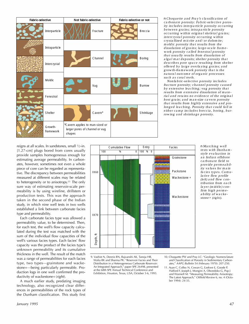
reigns at all scales. In sandstones, small 1/2-in.[1.27-cm] plugs bored from cores usuallyprovide samples homogeneous enough forestimating average permeability. In carbon-ates, however, sometimes not even a wholepiece of core can be regarded as representa-tive. The discrepancy between permeabilitiesmeasured at different scales may be relatedto heterogeneity or to anisotropy.11 The onlysure way of estimating reservoir-scale per-meability is by using wireline, drillstem orproduction tests. This was the approachtaken in the second phase of the Indianstudy, in which nine well tests in two wellsestablished a link between carbonate faciestype and permeability.
Each carbonate facies type was allowed apermeability value, to be determined. Then,for each test, the well’s flow capacity calcu-lated during the test was matched with thesum of the individual flow capacities of thewell’s various facies types. Each facies’ flowcapacity was the product of the facies type’sunknown permeability and its cumulativethickness in the well. The result of the matchwas a range of permeabilities for each faciestype, two types—grainstone and wacke-stone+—being particularly permeable. Pro-duction logs in one well confirmed the pro-ductivity of wackestone+ (right).
A much earlier study, predating imagingtechnology, also recognized clear differ-ences in permeabilities of the rock types ofthe Dunham classification. This study first
10. Choquette PW and Pray LC: “Geologic Nomenclatureand Classification of Porosity in Sedimentary Carbon-ates,” AAPG Bulletin 54 (February 1970): 207-250.
11. Ayan C, Colley N, Cowan G, Ezekwe E, Goode P,Halford F, Joseph J, Mongini A, Obondoko G, Pop Jand Wannell M: “Measuring Permeability Anisotropy:The Latest Approach,” Oilfield Review 6, no. 4 (Octo-ber 1994): 24-35.
9. Vashist N, Dennis RN, Rajvanshi AK, Taneja HR,Walia RK and Sharma PK: “Reservoir Facies and TheirDistribution in a Heterogeneous Carbonate Reservoir:An Integrated Approach,” paper SPE 26498, presentedat the 68th SPE Annual Technical Conference andExhibition, Houston, Texas, USA, October 3-6, 1993.
47January 1995
nChoquette and Pray’s classification ofcarbonate porosity: Fabric-selective poros-ity includes interparticle porosity occurringbetween grains; intraparticle porosityoccurring within original skeletal grains;intercrystal porosity occurring within crystallized micrite and/or dolomite;moldic porosity that results from the dissolution of grains; large-scale frame-work porosity called fenestral porosity that usually results from dissolution ofalgal mat deposits; shelter porosity thatdescribes pore space resulting from shelteroffered by large overlaying grains; andgrowth-framework porosity that is the natural outcome of organic processes such as coral reefs.
Nonfabric-selective porosity includesfracture porosity; channel porosity causedby extensive leaching; vug porosity thatresults from extensive dissolution of mate-rial and retains no evidence of the originalhost grain; and man-size cavern porositythat results from highly extensive and pro-longed leaching. Porosity that could fall ineither camp includes breccia, boring, bur-rowing and shrinkage porosity.
nMatching welltests with Dunham-style evaluation inan Indian offshorecarbonate field toprovide permeabil-ity values for mainfacies types. Cumu-lative flow profile(left) and flow con-tribution from eachlayer (middle) con-firm high perme-ability of wacke-stone+ (right).
Wackestone +
Wackestone
Cumulative Flow FaciesEntry
Packstone
Grainstone
Dep
th, f
t
XX60
100 % %100 00
XX70
Fabric-selective Not fabric-selective Fabric-selective or not
Interparticle
Intraparticle
Intercrystal
Moldic
Fenestral
Shelter
Growth-framework
Fracture
Channel
Vug
Cavern*
Breccia
Shrinkage
Burrow
Boring
*Cavern applies to man-sized or larger pores of channel or vug shapes
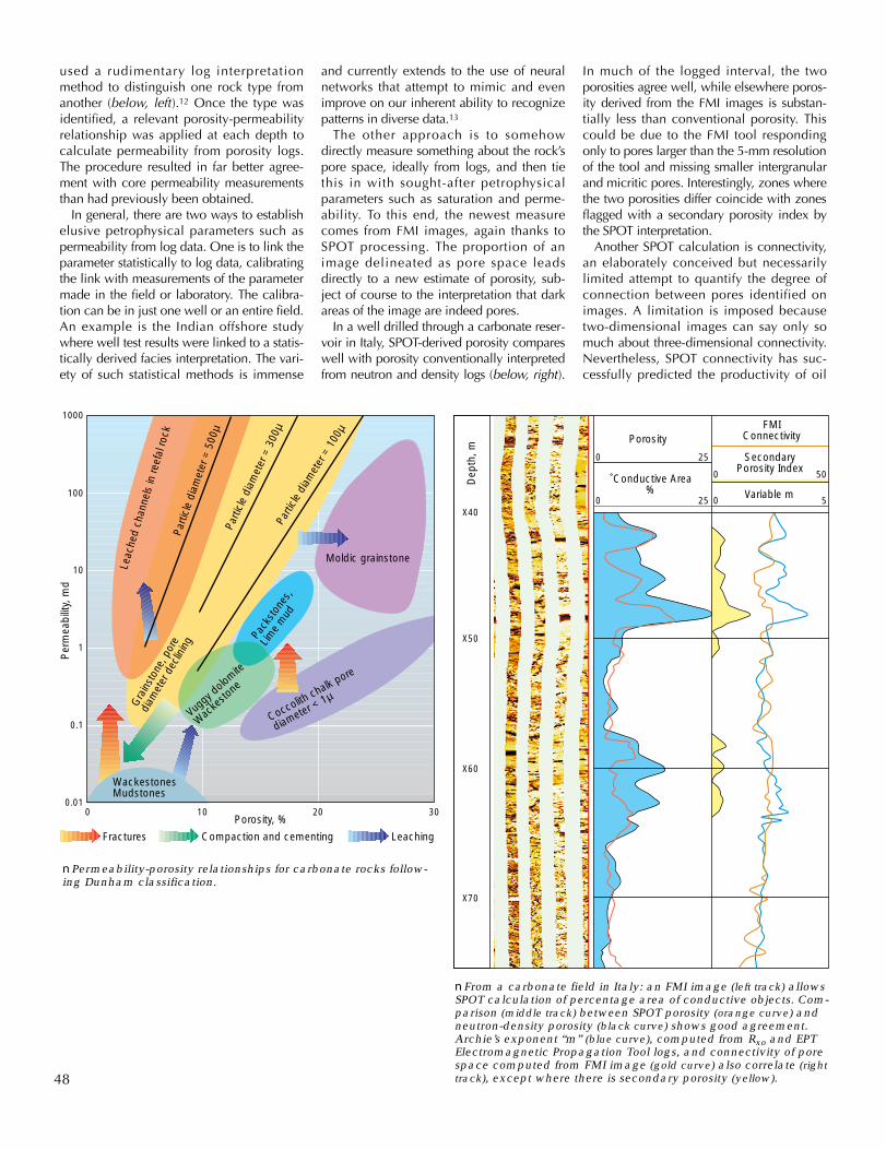
used a rudimentary log interpretationmethod to distinguish one rock type fromanother (below, left).12 Once the type wasidentified, a relevant porosity-permeabilityrelationship was applied at each depth tocalculate permeability from porosity logs.The procedure resulted in far better agree-ment with core permeability measurementsthan had previously been obtained.
In general, there are two ways to establishelusive petrophysical parameters such aspermeability from log data. One is to link theparameter statistically to log data, calibratingthe link with measurements of the parametermade in the field or laboratory. The calibra-tion can be in just one well or an entire field.An example is the Indian offshore studywhere well test results were linked to a statis-tically derived facies interpretation. The vari-ety of such statistical methods is immense
and currently extends to the use of neuralnetworks that attempt to mimic and evenimprove on our inherent ability to recognizepatterns in diverse data.13
The other approach is to somehowdirectly measure something about the rock’spore space, ideally from logs, and then tiethis in with sought-after petrophysicalparameters such as saturation and perme-ability. To this end, the newest measurecomes from FMI images, again thanks toSPOT processing. The proportion of animage delineated as pore space leadsdirectly to a new estimate of porosity, sub-ject of course to the interpretation that darkareas of the image are indeed pores.
In a well drilled through a carbonate reser-voir in Italy, SPOT-derived porosity compareswell with porosity conventionally interpretedfrom neutron and density logs (below, right).
In much of the logged interval, the twoporosities agree well, while elsewhere poros-ity derived from the FMI images is substan-tially less than conventional porosity. Thiscould be due to the FMI tool respondingonly to pores larger than the 5-mm resolutionof the tool and missing smaller intergranularand micritic pores. Interestingly, zones wherethe two porosities differ coincide with zonesflagged with a secondary porosity index bythe SPOT interpretation.
Another SPOT calculation is connectivity,an elaborately conceived but necessarilylimited attempt to quantify the degree ofconnection between pores identified onimages. A limitation is imposed becausetwo-dimensional images can say only somuch about three-dimensional connectivity.Nevertheless, SPOT connectivity has suc-cessfully predicted the productivity of oil
48
nPermeability-porosity relationships for carbonate rocks follow-ing Dunham classification.
nFrom a carbonate field in Italy: an FMI image (left track) allowsSPOT calculation of percentage area of conductive objects. Com-parison (middle track) between SPOT porosity (orange curve) andneutron-density porosity (black curve) shows good agreement.Archie’s exponent “m” (blue curve), computed from Rxo and EPTElectromagnetic Propagation Tool logs, and connectivity of porespace computed from FMI image (gold curve) also correlate (righttrack), except where there is secondary porosity (yellow).
Per
mea
bilit
y, m
d
1000
10
100
1
0.1
0.01
WackestonesMudstones
Vugg
y dolo
mite
Wacke
stone
Pack
ston
es,
Lime
mud
Gra
inst
one,
por
e
diam
eter
dec
linin
g
Moldic grainstone
Parti
cle d
iamet
er =
100
µ
Parti
cle
diam
eter
= 3
00µ
Par
ticle
dia
met
er =
500
µ
Leac
hed
chan
nels
in re
efal
rock
Coccolith chalk pore
diameter < 1µ
0 10 20 30Porosity, %
Fractures LeachingCompaction and cementing
Dep
th, m
X40
X50
X60
X70
0 25 0 5
0 50 Conductive Area%
Porosity
0 25
Variable m
SecondaryPorosity Index
FMIConnectivity
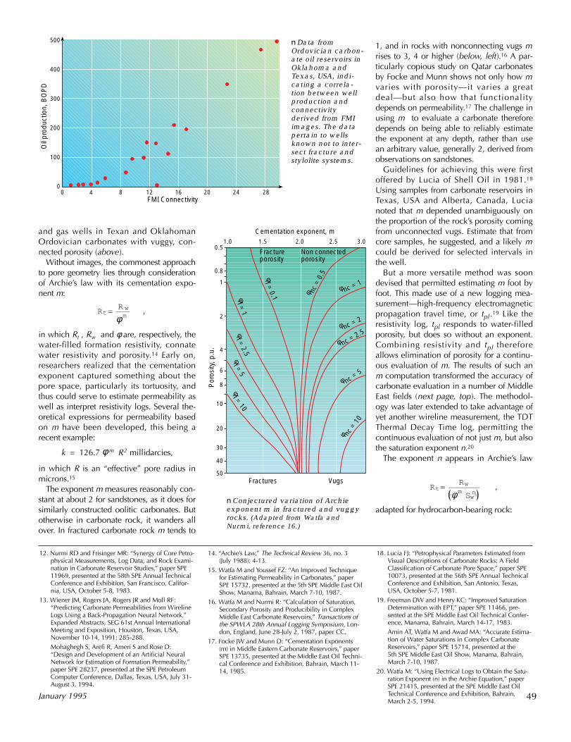
and gas wells in Texan and OklahomanOrdovician carbonates with vuggy, con-nected porosity (above).
Without images, the commonest approachto pore geometry lies through considerationof Archie’s law with its cementation expo-nent m:
in which Rt , Rw and φare, respectively, thewater-filled formation resistivity, connatewater resistivity and porosity.14 Early on,researchers realized that the cementationexponent captured something about thepore space, particularly its tortuosity, andthus could serve to estimate permeability aswell as interpret resistivity logs. Several the-oretical expressions for permeability basedon m have been developed, this being arecent example:
k = 126.7 φm R2 millidarcies,
in which R is an “effective” pore radius inmicrons.15
The exponent m measures reasonably con-stant at about 2 for sandstones, as it does forsimilarly constructed oolitic carbonates. Butotherwise in carbonate rock, it wanders allover. In fractured carbonate rock m tends to
1, and in rocks with nonconnecting vugs mrises to 3, 4 or higher (below, left).16 A par-ticularly copious study on Qatar carbonatesby Focke and Munn shows not only how mvaries with porosity—it varies a greatdeal—but also how that functionalitydepends on permeability.17 The challenge inusing m to evaluate a carbonate thereforedepends on being able to reliably estimatethe exponent at any depth, rather than usean arbitrary value, generally 2, derived fromobservations on sandstones.
Guidelines for achieving this were firstoffered by Lucia of Shell Oil in 1981.18
Using samples from carbonate reservoirs inTexas, USA and Alberta, Canada, Lucianoted that m depended unambiguously onthe proportion of the rock’s porosity comingfrom unconnected vugs. Estimate that fromcore samples, he suggested, and a likely mcould be derived for selected intervals inthe well.
But a more versatile method was soondevised that permitted estimating m foot byfoot. This made use of a new logging mea-surement—high-frequency electromagneticpropagation travel time, or tpl .19 Like theresistivity log, tpl responds to water-filledporosity, but does so without an exponent.Combining resistivity and tpl thereforeallows elimination of porosity for a continu-ous evaluation of m. The results of such anm computation transformed the accuracy ofcarbonate evaluation in a number of MiddleEast fields (next page, top). The methodol-ogy was later extended to take advantage ofyet another wireline measurement, the TDTThermal Decay Time log, permitting thecontinuous evaluation of not just m, but alsothe saturation exponent n.20
The exponent n appears in Archie’s law
adapted for hydrocarbon-bearing rock:
49January 1995
nData fromOrdovician carbon-ate oil reservoirs inOklahoma andTexas, USA, indi-cating a correla-tion between wellproduction andconnectivityderived from FMIimages. The datapertain to wellsknown not to inter-sect fracture andstylolite systems.
nConjectured variation of Archieexponent m in fractured and vuggyrocks. (Adapted from Watfa andNurmi, reference 16.)
12. Nurmi RD and Frisinger MR: “Synergy of Core Petro-physical Measurements, Log Data, and Rock Exami-nation in Carbonate Reservoir Studies,” paper SPE11969, presented at the 58th SPE Annual TechnicalConference and Exhibition, San Francisco, Califor-nia, USA, October 5-8, 1983.
13. Wiener JM, Rogers JA, Rogers JR and Moll RF: “Predicting Carbonate Permeabilities from Wireline Logs Using a Back-Propagation Neural Network,”Expanded Abstracts, SEG 61st Annual InternationalMeeting and Exposition, Houston, Texas, USA,November 10-14, 1991: 285-288.Mohaghegh S, Arefi R, Ameri S and Rose D: “Design and Development of an Artificial NeuralNetwork for Estimation of Formation Permeability,”paper SPE 28237, presented at the SPE PetroleumComputer Conference, Dallas, Texas, USA, July 31-August 3, 1994.
14. “Archie’s Law,” The Technical Review 36, no. 3 (July 1988): 4-13.
15. Watfa M and Youssef FZ: “An Improved Techniquefor Estimating Permeability in Carbonates,” paperSPE 15732, presented at the 5th SPE Middle East OilShow, Manama, Bahrain, March 7-10, 1987.
16. Watfa M and Nurmi R: “Calculation of Saturation,Secondary Porosity and Producibility in ComplexMiddle East Carbonate Reservoirs,” Transactions ofthe SPWLA 28th Annual Logging Symposium, Lon-don, England, June 28-July 2, 1987, paper CC.
17. Focke JW and Munn D: “Cementation Exponents (m) in Middle Eastern Carbonate Reservoirs,” paperSPE 13735, presented at the Middle East Oil Techni-cal Conference and Exhibition, Bahrain, March 11-14, 1985.
18. Lucia FJ: “Petrophysical Parameters Estimated fromVisual Descriptions of Carbonate Rocks: A FieldClassification of Carbonate Pore Space,” paper SPE10073, presented at the 56th SPE Annual TechnicalConference and Exhibition, San Antonio, Texas,USA, October 5-7, 1981.
19. Freeman DW and Henry KC: “Improved SaturationDetermination with EPT,” paper SPE 11466, pre-sented at the SPE Middle East Oil Technical Confer-ence, Manama, Bahrain, March 14-17, 1983.Amin AT, Watfa M and Awad MA: “Accurate Estima-tion of Water Saturations in Complex CarbonateReservoirs,” paper SPE 15714, presented at the 5th SPE Middle East Oil Show, Manama, Bahrain, March 7-10, 1987.
20. Watfa M: “Using Electrical Logs to Obtain the Satu-ration Exponent (n) in the Archie Equation,” paperSPE 21415, presented at the SPE Middle East OilTechnical Conference and Exhibition, Bahrain,March 2-5, 1994.
Rt = Rw
φm Swn ,
Rt = Rw
φm ,
28
Oil
prod
uctio
n, B
OP
D
0
FMI Connectivity
100
200
300
400
500
24201612840
1.0 1.5 2.0 2.5 3.0
Cementation exponent, m
Por
osity
, p.u
.
Fractures Vugs
Fractureporosity
φ nc =
10
50
40
30
20
10
8
6
4
2
1
0.8
0.5
φ nc = 5
φ nc = 2.5φ nc = 2
φ nc = 1
Non connectedporosity
φ nc =
0.5φ
f = 0.1φf = 1
φf = 2.5
φf = 5
φf = 10
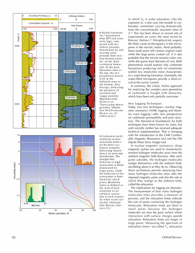
in which Sw is water saturation. Like theexponent m, n also runs into trouble in car-bonates, sometimes varying dramaticallyfrom the conventionally assumed value of2.21 This has been shown in several sets ofexperiments on cores, the most recent byBouvier (below).22 Petrophysicists suspectthe likely cause of discrepancy is tiny micro-pores in the micritic matrix. Most probably,these small pores still contain original waterwhile the large pores contain oil. It is alsoprobable that the micrite remains water wet,while the grains have become oil wet. Bothphenomena would explain why carbonateformations producing only oil sometimesexhibit low resistivities more characteristicof a water-bearing formation. Essentially, thewater-filled micropores provide a short-cir-cuit to the survey current.
In summary, the classic Archie approachfor analyzing the complex pore geometriesof carbonate is fraught with obstacles,which have been only partially overcome.
New Logging TechniquesToday, two new techniques—nuclear mag-netic resonance (NMR) logging and Stone-ley wave logging—offer new perspectiveson carbonate permeability and pore struc-ture. The theoretical foundations for bothtechniques have been known for years, butuntil recently neither has received adequatetechnical implementation. That is changingwith the introduction of the CMR Combin-able Magnetic Resonance tool and the DSIDipole Shear Sonic Imager tool.
In nuclear magnetic resonance, sharpmagnetic pulses are used to momentarilyreorient hydrogen molecules away from theambient magnetic field direction. After eachpulse subsides, the hydrogen moleculesrealign themselves with the ambient field,oscillating about it as they do so. Observingthese oscillations permits measuring howmany hydrogen molecules relax after theimposed magnetic pulse and also the rate atwhich they realign to the ambient field,called the relaxation.
The implications for logging are dramatic.The measurement of how many hydrogenmolecules relax provides a measure ofporosity, and the relaxation times indicatethe size of pores containing the hydrogenmolecules. Relaxation times are short insmall pores because the hydrogenmolecules are near the grain surface whereinteraction with surface charges speedsrelaxation. Relaxation times are longer inlarge pores. Measuring the spectrum ofrelaxation times—so-called T2 relaxation
50 Oilfield Review
nArchie exponent“m,” determinedfrom EPT and resis-tivity logs, com-pared with sec-ondary porosity,determined by sub-tracting sonicporosity from neu-tron-density poros-ity—in the Arabcarbonate forma-tion. In the purelimestone zone atthe top, the twoparameters matchwell. In thedolomite zone atthe bottom, theydiverge, indicatingthe presence ofunconnectedvuggy porosity.[Reprinted fromNurmi et al.: “Typecasting Hetero-geneities,” MiddleEast Well EvaluationReview, no. 10(1991):16-32.]
nCarbonate rock’sresistivity-versus-saturation behav-ior for three car-bonate samples,indicating depen-dence on pore-sizedistribution. Thestraight-linebehavior at highsaturations is likelydominated bylarge pores, whilethe behavior at lowsaturations is dom-inated by smallpores. Resistivityindex is defined asthe ratio of rockresistivity at anarbitrary satura-tion to rock resistiv-ity when water sat-urated. (Adaptedfrom Bouvier, refer-ence 22.)
50
Res
istiv
ity in
dex
Water saturation, %
10
60 70 80 90 100
8
6
4
2.5
1.5
1Microns
0.04 63
XX00
2.00
0 Secondary Porosity, p.u.
Cementation Exponent, m
Lithology Analysis
Fluid Volume
25
100.00
0 100
%
%
Residual oil
Moved oil
Limestone
Dolomite
Water
0.007.00
Dep
th, f
t
XX50
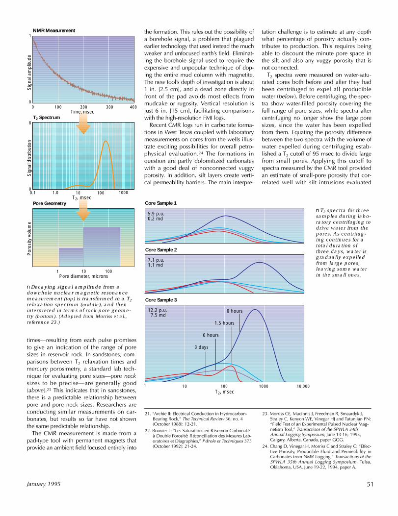
7.1 p.u.1.1 md
Core Sample 2
5.9 p.u.0.2 md
Core Sample 1
T2, msec10,0001000100101
12.2 p.u. 7.5 md
3 days
6 hours
1.5 hours
0 hours
Core Sample 3
times—resulting from each pulse promisesto give an indication of the range of poresizes in reservoir rock. In sandstones, com-parisons between T2 relaxation times andmercury porosimetry, a standard lab tech-nique for evaluating pore sizes—pore necksizes to be precise—are generally good(above).23 This indicates that in sandstones,there is a predictable relationship betweenpore and pore neck sizes. Researchers areconducting similar measurements on car-bonates, but results so far have not shownthe same predictable relationship.
The CMR measurement is made from apad-type tool with permanent magnets thatprovide an ambient field focused entirely into
the formation. This rules out the possibility ofa borehole signal, a problem that plaguedearlier technology that used instead the muchweaker and unfocused earth’s field. Eliminat-ing the borehole signal used to require theexpensive and unpopular technique of dop-ing the entire mud column with magnetite.The new tool’s depth of investigation is about1 in. [2.5 cm], and a dead zone directly infront of the pad avoids most effects frommudcake or rugosity. Vertical resolution isjust 6 in. [15 cm], facilitating comparisonswith the high-resolution FMI logs.
Recent CMR logs run in carbonate forma-tions in West Texas coupled with laboratorymeasurements on cores from the wells illus-trate exciting possibilities for overall petro-physical evaluation.24 The formations inquestion are partly dolomitized carbonateswith a good deal of nonconnected vuggyporosity. In addition, silt layers create verti-cal permeability barriers. The main interpre-
tation challenge is to estimate at any depthwhat percentage of porosity actually con-tributes to production. This requires beingable to discount the minute pore space inthe silt and also any vuggy porosity that isnot connected.
T2 spectra were measured on water-satu-rated cores both before and after they hadbeen centrifuged to expel all produciblewater (below). Before centrifuging, the spec-tra show water-filled porosity covering thefull range of pore sizes, while spectra aftercentrifuging no longer show the large poresizes, since the water has been expelledfrom them. Equating the porosity differencebetween the two spectra with the volume ofwater expelled during centrifuging estab-lished a T2 cutoff of 95 msec to divide largefrom small pores. Applying this cutoff tospectra measured by the CMR tool providedan estimate of small-pore porosity that cor-related well with silt intrusions evaluated
51January 1995
21. “Archie II: Electrical Conduction in Hydrocarbon-Bearing Rock,” The Technical Review 36, no. 4(October 1988): 12-21.
22. Bouvier L: “Les Saturations en Réservoir Carbonatéà Double Porosité: Réconciliation des Mesures Lab-oratoires et Diagraphies,” Pétrole et Techniques 375(October 1992): 21-24.
23. Morriss CE, MacInnis J, Freedman R, Smaardyk J,Straley C, Kenyon WE, Vinegar HJ and Tutunjian PN:“Field Test of an Experimental Pulsed Nuclear Mag-netism Tool,” Transactions of the SPWLA 34thAnnual Logging Symposium, June 13-16, 1993,Calgary, Alberta, Canada, paper GGG.
24. Chang D, Vinegar H, Morriss C and Straley C: “Effec-tive Porosity, Producible Fluid and Permeability inCarbonates from NMR Logging,” Transactions of theSPWLA 35th Annual Logging Symposium, Tulsa,Oklahoma, USA, June 19-22, 1994, paper A.
nT2 spectra for threesamples during labo-ratory centrifuging todrive water from thepores. As centrifug-ing continues for atotal duration ofthree days, water isgradually expelledfrom large pores,leaving some waterin the small ones.
nDecaying signal amplitude from adownhole nuclear magnetic resonancemeasurement (top) is transformed to a T2relaxation spectrum (middle), and theninterpreted in terms of rock pore geome-try (bottom). (Adapted from Morriss et al.,reference 23.)
Sig
nal a
mpl
itude
0 100 200 300 400
Sig
nal d
istri
butio
n
0.1 1.0 10 100 1000
Por
osity
vol
ume
Pore diameter, microns1 10 100
NMR Measurement
T2 Spectrum
Pore Geometry
Time, msec
T2, msec
0
1
0
8
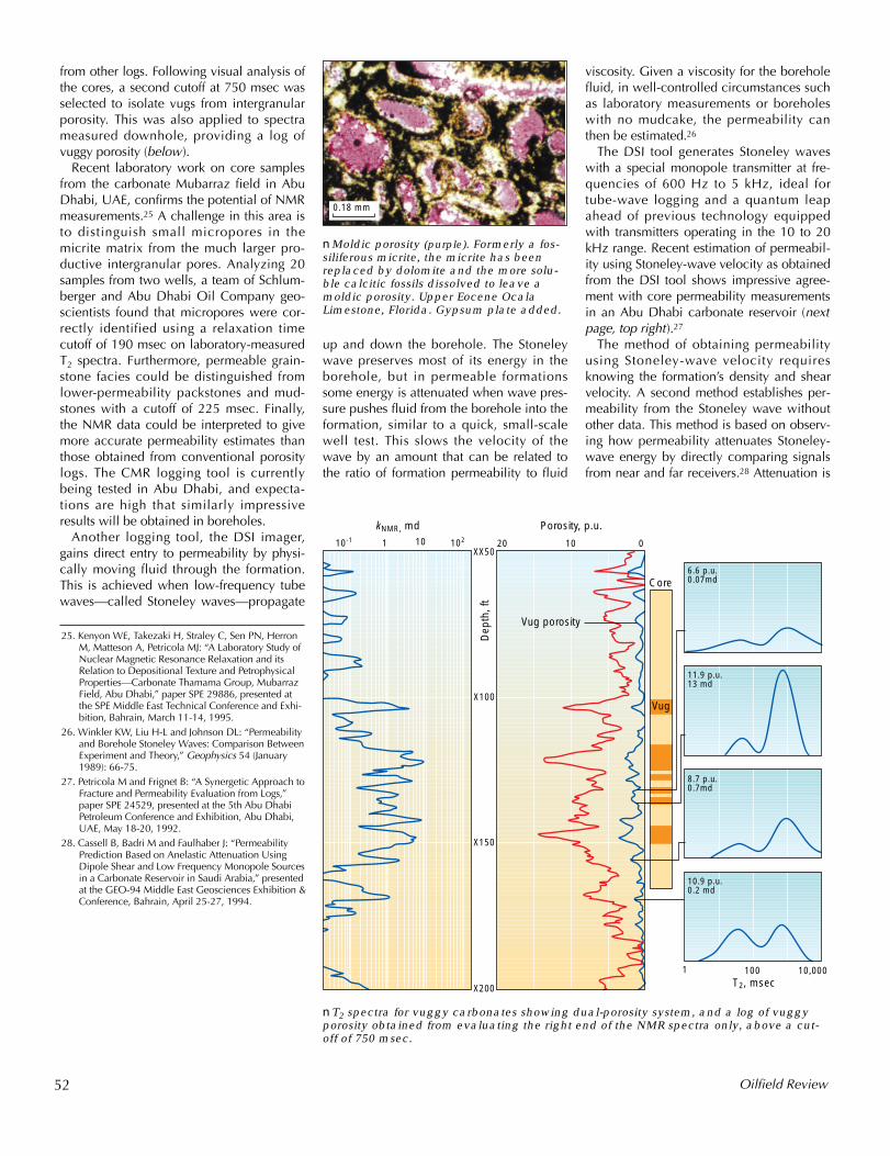
from other logs. Following visual analysis ofthe cores, a second cutoff at 750 msec wasselected to isolate vugs from intergranularporosity. This was also applied to spectrameasured downhole, providing a log ofvuggy porosity (below).
Recent laboratory work on core samplesfrom the carbonate Mubarraz field in AbuDhabi, UAE, confirms the potential of NMRmeasurements.25 A challenge in this area isto distinguish small micropores in themicrite matrix from the much larger pro-ductive intergranular pores. Analyzing 20samples from two wells, a team of Schlum-berger and Abu Dhabi Oil Company geo-scientists found that micropores were cor-rectly identified using a relaxation timecutoff of 190 msec on laboratory-measuredT2 spectra. Furthermore, permeable grain-stone facies could be distinguished fromlower-permeability packstones and mud-stones with a cutoff of 225 msec. Finally,the NMR data could be interpreted to givemore accurate permeability estimates thanthose obtained from conventional porositylogs. The CMR logging tool is currentlybeing tested in Abu Dhabi, and expecta-tions are high that similarly impressiveresults will be obtained in boreholes.
Another logging tool, the DSI imager,gains direct entry to permeability by physi-cally moving fluid through the formation.This is achieved when low-frequency tubewaves—called Stoneley waves—propagate
up and down the borehole. The Stoneleywave preserves most of its energy in theborehole, but in permeable formationssome energy is attenuated when wave pres-sure pushes fluid from the borehole into theformation, similar to a quick, small-scalewell test. This slows the velocity of thewave by an amount that can be related tothe ratio of formation permeability to fluid
52 Oilfield Review
nMoldic porosity (purple). Formerly a fos-siliferous micrite, the micrite has beenreplaced by dolomite and the more solu-ble calcitic fossils dissolved to leave amoldic porosity. Upper Eocene OcalaLimestone, Florida. Gypsum plate added.
nT2 spectra for vuggy carbonates showing dual-porosity system, and a log of vuggyporosity obtained from evaluating the right end of the NMR spectra only, above a cut-off of 750 msec.
25. Kenyon WE, Takezaki H, Straley C, Sen PN, HerronM, Matteson A, Petricola MJ: “A Laboratory Study ofNuclear Magnetic Resonance Relaxation and itsRelation to Depositional Texture and PetrophysicalProperties—Carbonate Thamama Group, MubarrazField, Abu Dhabi,” paper SPE 29886, presented atthe SPE Middle East Technical Conference and Exhi-bition, Bahrain, March 11-14, 1995.
26. Winkler KW, Liu H-L and Johnson DL: “Permeabilityand Borehole Stoneley Waves: Comparison BetweenExperiment and Theory,” Geophysics 54 (January1989): 66-75.
27. Petricola M and Frignet B: “A Synergetic Approach toFracture and Permeability Evaluation from Logs,”paper SPE 24529, presented at the 5th Abu DhabiPetroleum Conference and Exhibition, Abu Dhabi,UAE, May 18-20, 1992.
28. Cassell B, Badri M and Faulhaber J: “PermeabilityPrediction Based on Anelastic Attenuation UsingDipole Shear and Low Frequency Monopole Sourcesin a Carbonate Reservoir in Saudi Arabia,” presentedat the GEO-94 Middle East Geosciences Exhibition &Conference, Bahrain, April 25-27, 1994.
viscosity. Given a viscosity for the boreholefluid, in well-controlled circumstances suchas laboratory measurements or boreholeswith no mudcake, the permeability canthen be estimated.26
The DSI tool generates Stoneley waveswith a special monopole transmitter at fre-quencies of 600 Hz to 5 kHz, ideal fortube-wave logging and a quantum leapahead of previous technology equippedwith transmitters operating in the 10 to 20kHz range. Recent estimation of permeabil-ity using Stoneley-wave velocity as obtainedfrom the DSI tool shows impressive agree-ment with core permeability measurementsin an Abu Dhabi carbonate reservoir (nextpage, top right).27
The method of obtaining permeabilityusing Stoneley-wave velocity requiresknowing the formation’s density and shearvelocity. A second method establishes per-meability from the Stoneley wave withoutother data. This method is based on observ-ing how permeability attenuates Stoneley-wave energy by directly comparing signalsfrom near and far receivers.28 Attenuation is
8.7 p.u.0.7md
X200
X150
X100
XX5010-1 1 10 102
kNMR, md
20
Porosity, p.u.
10 0
Core
Vug porosity
Vug
1 100 10,000T2, msec
11.9 p.u.13 md
10.9 p.u.0.2 md
6.6 p.u.0.07md
Dep
th, f
t
0.18 mm
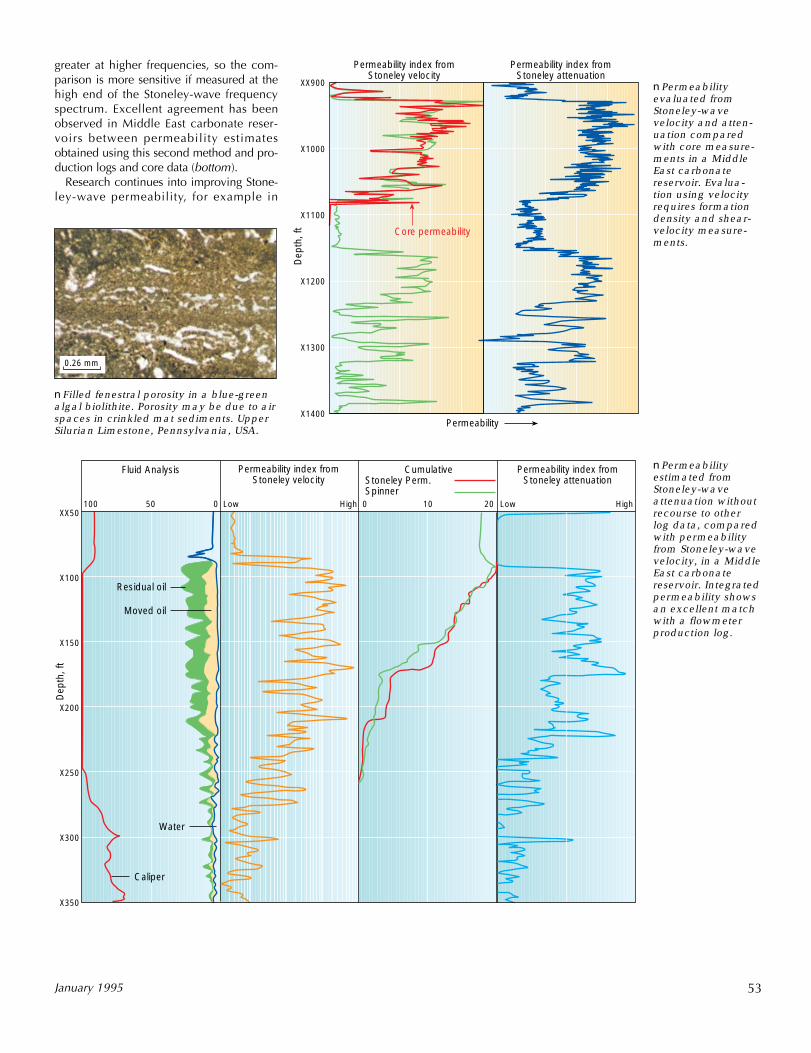
greater at higher frequencies, so the com-parison is more sensitive if measured at thehigh end of the Stoneley-wave frequencyspectrum. Excellent agreement has beenobserved in Middle East carbonate reser-voirs between permeability estimatesobtained using this second method and pro-duction logs and core data (bottom).
Research continues into improving Stone-ley-wave permeability, for example in
53January 1995
nFilled fenestral porosity in a blue-greenalgal biolithite. Porosity may be due to airspaces in crinkled mat sediments. UpperSilurian Limestone, Pennsylvania, USA.
XX50
Fluid Analysis
X100
X150
X200
X250
X300
X350
Dep
th, f
t
100 50 0 Low High
Permeability index fromStoneley velocity
CumulativeStoneley Perm.Spinner
Permeability index fromStoneley attenuation
HighLow0 10 20
Residual oil
Moved oil
Water
Caliper
Permeability index fromStoneley velocity
Permeability index fromStoneley attenuation
XX900
X1000
X1100
X1200
X1300
X1400
Dep
th, f
t Core permeability
Permeability
nPermeability estimated fromStoneley-wave attenuation withoutrecourse to other log data, comparedwith permeabilityfrom Stoneley-wavevelocity, in a MiddleEast carbonatereservoir. Integratedpermeability showsan excellent matchwith a flowmeterproduction log.
nPermeabilityevaluated fromStoneley-wavevelocity and atten-uation comparedwith core measure-ments in a MiddleEast carbonatereservoir. Evalua-tion using velocityrequires formationdensity and shear-velocity measure-ments.
0.26 mm
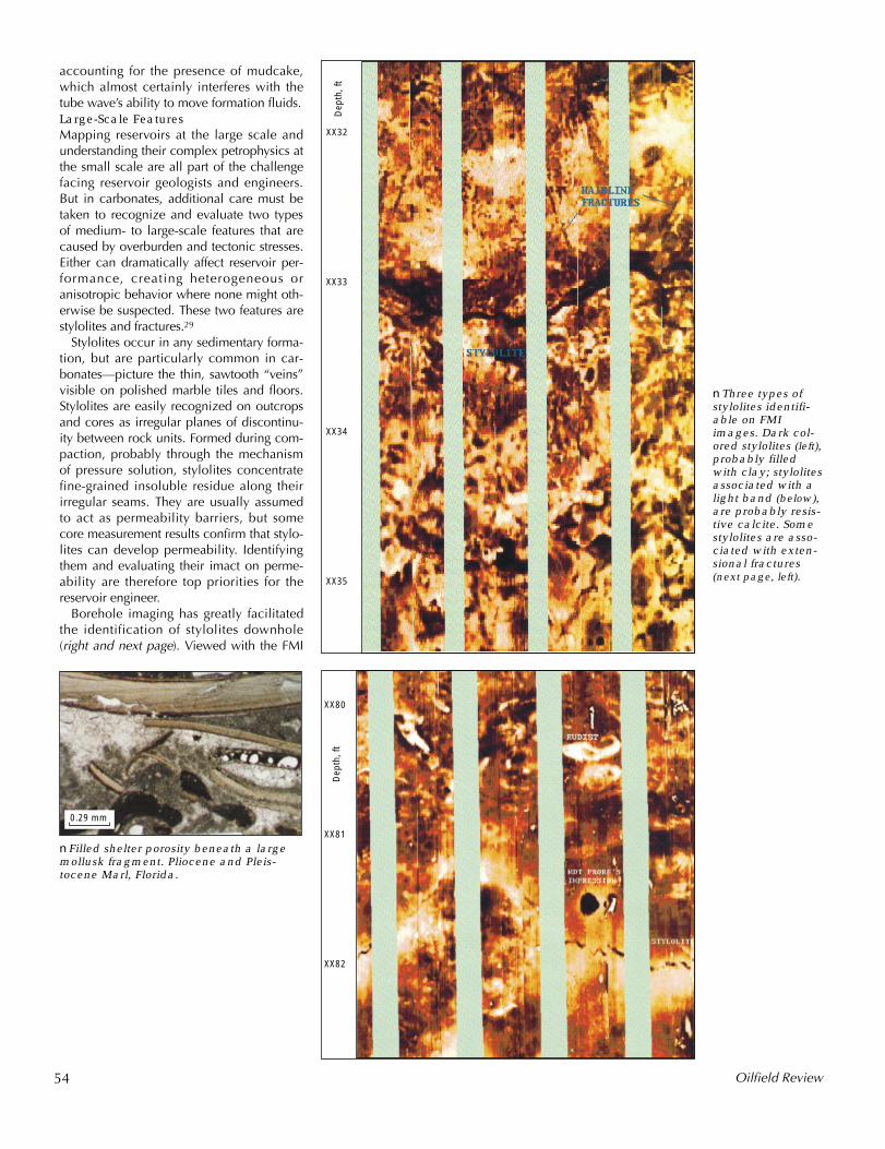
accounting for the presence of mudcake,which almost certainly interferes with thetube wave’s ability to move formation fluids.Large-Scale FeaturesMapping reservoirs at the large scale andunderstanding their complex petrophysics atthe small scale are all part of the challengefacing reservoir geologists and engineers.But in carbonates, additional care must betaken to recognize and evaluate two typesof medium- to large-scale features that arecaused by overburden and tectonic stresses.Either can dramatically affect reservoir per-formance, creating heterogeneous oranisotropic behavior where none might oth-erwise be suspected. These two features arestylolites and fractures.29
Stylolites occur in any sedimentary forma-tion, but are particularly common in car-bonates—picture the thin, sawtooth “veins”visible on polished marble tiles and floors.Stylolites are easily recognized on outcropsand cores as irregular planes of discontinu-ity between rock units. Formed during com-paction, probably through the mechanismof pressure solution, stylolites concentratefine-grained insoluble residue along theirirregular seams. They are usually assumedto act as permeability barriers, but somecore measurement results confirm that stylo-lites can develop permeability. Identifyingthem and evaluating their imact on perme-ability are therefore top priorities for thereservoir engineer.
Borehole imaging has greatly facilitatedthe identification of stylolites downhole(right and next page). Viewed with the FMI
54 Oilfield Review
nFilled shelter porosity beneath a largemollusk fragment. Pliocene and Pleis-tocene Marl, Florida.
nThree types ofstylolites identifi-able on FMIimages. Dark col-ored stylolites (left),probably filledwith clay; stylolitesassociated with alight band (below),are probably resis-tive calcite. Somestylolites are asso-ciated with exten-sional fractures(next page, left).
0.29 mm
XX32
XX33
XX34
XX35
Dep
th, f
t
XX80
XX81
XX82
Dep
th, f
t
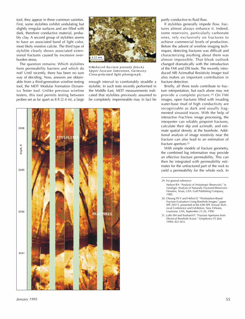
tool, they appear in three common varieties.First, some stylolites exhibit undulating butslightly irregular surfaces and are filled withdark, therefore conductive material, proba-bly clay. A second group of stylolites seemsto have an associated band of light color,most likely resistive calcite. The third type ofstylolite clearly shows associated exten-sional fractures caused by excessive over-burden stress.
The question remains: Which stylolitesform permeability barriers and which donot? Until recently, there has been no sureway of deciding. Now, answers are obtain-able from a third-generation wireline testingtool, the MDT Modular Formation Dynam-ics Tester tool. Unlike previous wirelinetesters, this tool permits testing betweenprobes set as far apart as 8 ft [2.4 m], a large
enough interval to comfortably straddle astylolite. In such tests recently performed inthe Middle East, MDT measurements indi-cated that stylolites previously assumed tobe completely impermeable may in fact be
partly conductive to fluid flow.If stylolites generally impede flow, frac-
tures almost always enhance it. Indeed,some reservoirs, particularly carbonateones, rely exclusively on fractures toachieve commercial levels of production.Before the advent of wireline imaging tech-niques, detecting fractures was difficult andcharacterizing anything about them wasalmost impossible. That bleak outlookchanged dramatically with the introductionof the FMI and DSI tools. The recently intro-duced ARI Azimuthal Resistivity Imager toolalso makes an important contribution infracture detection.
Briefly, all three tools contribute to frac-ture interpretation, but each alone may notprovide a complete picture.30 On FMIimages, open fractures filled with invadingwater-base mud of high conductivity arerecognizable as dark and usually frag-mented sinusoid traces. With the help ofinteractive FracView image processing, theinterpreter can reliably pinpoint fractures,calculate their dip and azimuth, and esti-mate spatial density at the borehole. Addi-tional analysis of image resistivity near thefracture can also lead to an estimation offracture aperture.31
With simple models of fracture geometry,the combined log information may providean effective fracture permeability. This canthen be integrated with permeability esti-mates for the unfractured part of the rock toyield a permeability for the whole rock. In
55January 1995
nReduced fracture porosity (black). Upper Jurassic Limestone, Germany.Cross-polarized light photograph.
29. For general reference:Nelson RA: “Analysis of Anisotropic Reservoirs,” inGeologic Analysis of Naturally Fractured Reservoirs.Houston, Texas, USA: Gulf Publishing Company,1985.
30. Cheung PS-Y and Heliot D: “Workstation-BasedFracture Evaluation Using Borehole Images,” paperSPE 20573, presented at the 65th SPE Annual Tech-nical Conference and Exhibition, New Orleans,Louisiana, USA, September 23-26, 1990.
31. Luthi SM and Souhaité P: “Fracture Apertures fromElectrical Borehole Scans,” Geophysics 55 (July1990): 821-833.
0.22 mm
XX88
XX89
XX90
Dep
th, f
t
XX91
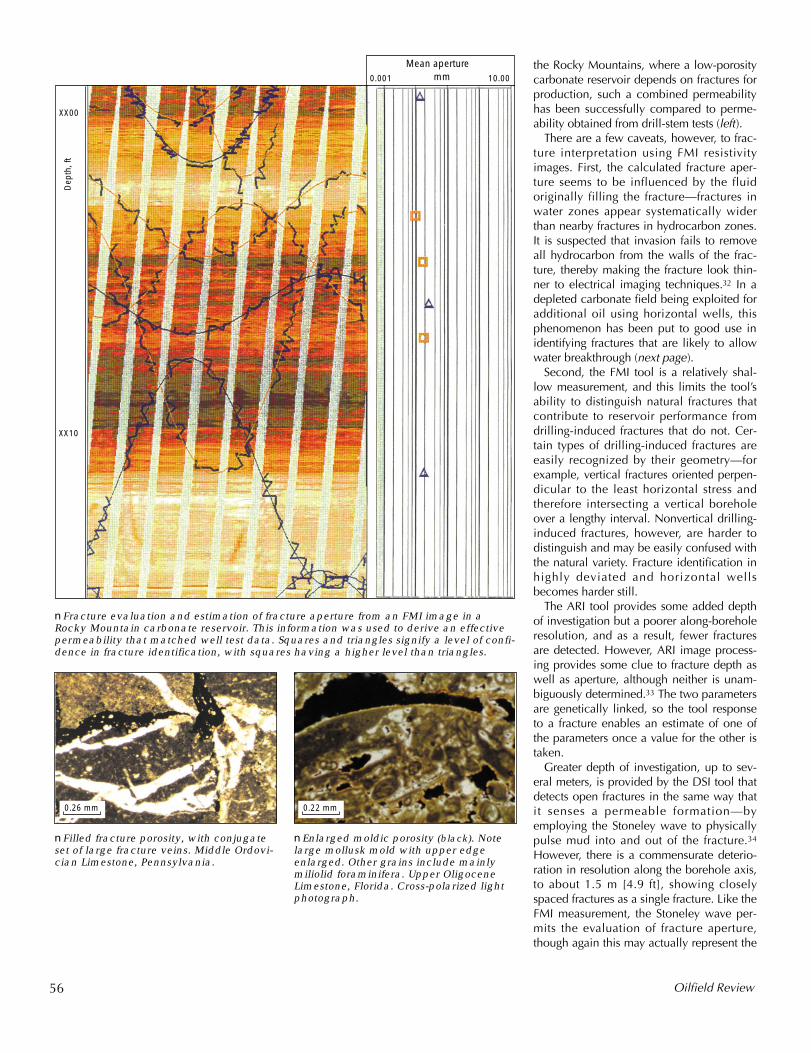
the Rocky Mountains, where a low-porositycarbonate reservoir depends on fractures forproduction, such a combined permeabilityhas been successfully compared to perme-ability obtained from drill-stem tests (left).
There are a few caveats, however, to frac-ture interpretation using FMI resistivityimages. First, the calculated fracture aper-ture seems to be influenced by the fluidoriginally filling the fracture—fractures inwater zones appear systematically widerthan nearby fractures in hydrocarbon zones.It is suspected that invasion fails to removeall hydrocarbon from the walls of the frac-ture, thereby making the fracture look thin-ner to electrical imaging techniques.32 In adepleted carbonate field being exploited foradditional oil using horizontal wells, thisphenomenon has been put to good use inidentifying fractures that are likely to allowwater breakthrough (next page).
Second, the FMI tool is a relatively shal-low measurement, and this limits the tool’sability to distinguish natural fractures thatcontribute to reservoir performance fromdrilling-induced fractures that do not. Cer-tain types of drilling-induced fractures areeasily recognized by their geometry—forexample, vertical fractures oriented perpen-dicular to the least horizontal stress andtherefore intersecting a vertical boreholeover a lengthy interval. Nonvertical drilling-induced fractures, however, are harder todistinguish and may be easily confused withthe natural variety. Fracture identification inhighly deviated and horizontal wellsbecomes harder still.
The ARI tool provides some added depthof investigation but a poorer along-boreholeresolution, and as a result, fewer fracturesare detected. However, ARI image process-ing provides some clue to fracture depth aswell as aperture, although neither is unam-biguously determined.33 The two parametersare genetically linked, so the tool responseto a fracture enables an estimate of one ofthe parameters once a value for the other istaken.
Greater depth of investigation, up to sev-eral meters, is provided by the DSI tool thatdetects open fractures in the same way thatit senses a permeable formation—byemploying the Stoneley wave to physicallypulse mud into and out of the fracture.34
However, there is a commensurate deterio-ration in resolution along the borehole axis,to about 1.5 m [4.9 ft], showing closelyspaced fractures as a single fracture. Like theFMI measurement, the Stoneley wave per-mits the evaluation of fracture aperture,though again this may actually represent the
56 Oilfield Review
nFracture evaluation and estimation of fracture aperture from an FMI image in aRocky Mountain carbonate reservoir. This information was used to derive an effectivepermeability that matched well test data. Squares and triangles signify a level of confi-dence in fracture identification, with squares having a higher level than triangles.
nFilled fracture porosity, with conjugateset of large fracture veins. Middle Ordovi-cian Limestone, Pennsylvania.
nEnlarged moldic porosity (black). Notelarge mollusk mold with upper edgeenlarged. Other grains include mainlymiliolid foraminifera. Upper OligoceneLimestone, Florida. Cross-polarized lightphotograph.
0.26 mm 0.22 mm
Mean aperture
XX00
XX10
0.001 mm 10.00D
epth
, ft
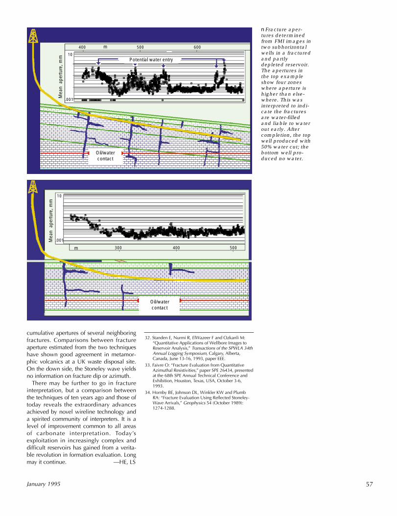
cumulative apertures of several neighboringfractures. Comparisons between fractureaperture estimated from the two techniqueshave shown good agreement in metamor-phic volcanics at a UK waste disposal site.On the down side, the Stoneley wave yieldsno information on fracture dip or azimuth.
There may be further to go in fractureinterpretation, but a comparison betweenthe techniques of ten years ago and those oftoday reveals the extraordinary advancesachieved by novel wireline technology anda spirited community of interpreters. It is alevel of improvement common to all areasof carbonate interpretation. Today’sexploitation in increasingly complex anddifficult reservoirs has gained from a verita-ble revolution in formation evaluation. Longmay it continue. —HE, LS
57January 1995
nFracture aper-tures determinedfrom FMI images intwo subhorizontalwells in a fracturedand partlydepleted reservoir.The apertures inthe top exampleshow four zoneswhere aperture ishigher than else-where. This wasinterpreted to indi-cate the fracturesare water-filledand liable to waterout early. Aftercompletion, the topwell produced with50% water cut; thebottom well pro-duced no water.
32. Standen E, Nurmi R, ElWazeer F and Ozkanli M:“Quantitative Applications of Wellbore Images toReservoir Analysis,” Transactions of the SPWLA 34thAnnual Logging Symposium, Calgary, Alberta,Canada, June 13-16, 1993, paper EEE.
33. Faivre O: “Fracture Evaluation from QuantitativeAzimuthal Resistivities,” paper SPE 26434, presentedat the 68th SPE Annual Technical Conference andExhibition, Houston, Texas, USA, October 3-6,1993.
34. Hornby BE, Johnson DL, Winkler KW and PlumbRA: “Fracture Evaluation Using Reflected Stoneley-Wave Arrivals,” Geophysics 54 (October 1989):1274-1288.
Oil/watercontact
Potential water entry
Oil/watercontact
m
Mea
n a
pert
ure,
mm
300
.001
10
Mea
n a
pert
ure,
mm
.001
10
400 500
400 500 600m