Introduction to computability logic

(pre-print version)

The official version is published in Annals of Pure and Applied Logic, volume 123 (2003), pages 1-99

Giorgi Japaridze∗

Department of Computing Sciences, Villanova University,800 Lancaster Avenue, Villanova, PA 19085, USA

Email: giorgi.japaridze@villanova.eduURL: http://www.csc.villanova.edu/∼japaridz

Abstract

This work is an attempt to lay foundations for a theory of interactive computation and bring logicand theory of computing closer together. It semantically introduces a logic of computability and sets aprogram for studying various aspects of that logic. The intuitive notion of (interactive) computationalproblems is formalized as a certain new, procedural-rule-free sort of games (called static games) betweenthe machine and the environment, and computability is understood as existence of an interactive Turingmachine that wins the game against any possible environment. The formalism used as a specificationlanguage for computational problems, called the universal language, is a non-disjoint union of the for-malisms of classical, intuitionistic and linear logics, with logical operators interpreted as certain, — mostbasic and natural, — operations on problems. Validity of a formula is understood as being “alwayscomputable”, and the set of all valid formulas is called the universal logic. The name “universal” isrelated to the potential of this logic to integrate, on the basis of one semantics, classical, intuitionisticand linear logics, with their seemingly unrelated or even antagonistic philosophies. In particular, theclassical notion of truth turns out to be nothing but computability restricted to the formulas of theclassical fragment of the universal language, which makes classical logic a natural syntactic fragmentof the universal logic. The same appears to be the case for intuitionistic and linear logics (understoodin a broad sense and not necessarily identified with the particular known axiomatic systems). Unlikeclassical logic, these two do not have a good concept of truth, and the notion of computability restrictedto the corresponding two fragments of the universal language, based on the intuitions that it formalizes,can well qualify as “intuitionistic truth” and “linear-logic truth”. The paper also provides illustrationsof potential applications of the universal logic in knowledgebase, resourcebase and planning systems, aswell as constructive applied theories. The author has tried to make this article easy to read. It is fullyself-contained and can be understood without any specialized knowledge of any particular subfield oflogic or computer science.

MSC: primary: 03B47; secondary: 03F50; 03B70; 68Q10; 68T27; 68T30; 91A05

Keywords: Computability logic; Interactive computation; Game semantics; Linear logic; Intuitionistic logic;Knowledgebase

∗This material is based upon work supported by the National Science Foundation under Grant No. 0208816

1

Contents

1 Introduction 3

I Computational problems, i.e. games 7

2 Formal definition of games 7

3 Structural game properties 9

4 Static games 11

5 The arity of a game 14

6 Predicates as elementary games 15

7 Substitution of variables; instantiation 16

8 Prefixation; the depth of a game 17

9 Negation; trivial games 18

10 Choice (additive) operations 19

11 Blind operations 22

12 Parallel (multiplicative) operations 23

13 Branching (exponential) operations 26

14 Summary of game operation properties 34

II Computability, i.e. winnability 34

15 The hard-play model 35

16 The easy-play model 38

17 Equivalence of the hard- and easy-play models for static games 41

18 Algorithmic vs nonalgorithmic winnability 43

19 Reducibility 48

20 User’s strategies formalized 49

III The logic of computability 51

21 Basic closure properties of computability 52

22 A glance at some valid principles of computability 54

23 Universal problems 56

24 The universal language 58

2

25 The universal logic 60

26 Applications in knowledgebase and resourcebase systems 63

27 From syntax to semantics or vice versa? 67

28 Why study computability logic? 69

1 Introduction

Computability, i.e. algorithmic solvability, is certainly one of the most interesting concepts in mathematicsand computer science, and it would be more than natural to ask the question about what logic it induces.The goal of this paper is to introduce a basic logic of computability and provide a solid formal ground forfuture, more advanced, studies of this exciting subject.

Computability is a property of computational problems, or problems for short, sometimes also referredto as computational tasks. They can be thought of as dialogues, or games between two agents. The moststandard types of problems are short, two-step dialogues, consisting of asking a question (input) and givingan answer (output). However, there is no call for restricting the length of dialogues to only two steps: anymore or less advanced and systematic study of computational problems sooner or later will face the necessityto consider problems of higher degrees or interactivity. After all, most of the tasks that real computers andcomputer networks perform are truly interactive! In this paper by a computational problem we always meanan interactive problem that can be an arbitrarily (including infinitely) long dialogue; moreover, as this willbe seen shortly, we do not exclude “dialogues” of length less than 2, either.

The following few sections introduce a concept of games that presents a formalization of our intuitivenotion of (interactive) computational problems, thus providing us with a clear formal basis for studyingtheir algorithmic solvability. After defining a natural set of basic game operations and elaborating thecorresponding logic, we can obtain a tool for deeper and more systematic understanding of computationalproblems and relations between them, such as, say, the relation of reducibility of one problem to another, orthe property of decidability, both generalized to complex, interactive problems. What follows below in thissection is an informal explanation of our approach.

We understand computational problems as games between two players: the machine (agent) and the user(environment). While the game-playing behavior of the latter can be arbitrary, the machine, as its namesuggests, only can follow algorithmic strategies, — strategies implementable as computer programs. As asimple example, consider the problem of computing the value of function f . In the formalism that we aregoing to employ, this problem would be expressed by the formula

uxty(y = f(x)

).

It stands for a two-move-deep game, where the first move, — selecting a particular value m for x, — mustbe made by the user, and the second move, — selecting a value n for y, — by the machine. The game is thenconsidered won by the machine, i.e., the problem solved, if n really equals f(m). Obviously computabilityof f means nothing but existence of a machine that wins the game uxty

(y = f(x)

)against any possible

(behavior of the) user.Generally, uxA(x) is a game where the user has to make the first move by selecting a particular value m

for x, after which the play continues, — and the winner is determined, — according to the rules of A(m); ifthe user fails to make an initial move, the game is considered won by the machine as there was no particular(sub)problem specified by its adversary that it failed to solve. txA(x) is defined in the same way, only hereit is the machine who makes an initial move/choice. This interpretation makes t a constructive version ofexistential quantifier, while u is a constructive version of universal quantifier.

As for atomic formulas, such as n = f(m), they can be understood as games without any moves. We callthis sort of games elementary. An elementary game is automatically won or lost by the machine dependingon whether the formula representing it is true or false (true=won, false=lost). This interpretation makesthe classical concept of predicates a special case of games, and classical logic a special case of computabilitylogic.

3

The meanings of the propositional counterparts t and u of t and u must be easy to guess. They, too,signify a choice by the corresponding player. The only difference is that while in the case of t and u thechoice is made among the objects of the universe of discourse, t and u mean a choice between left and right.For example, the problem of deciding language L could be expressed by

ux(x ∈ L t x 6∈ L

),

denoting the game where the user has to select a string s as a value of x, to which the machine should replyby one of the moves left or right; the game will be considered won by the machine if s ∈ L and the moveleft was made or s 6∈ L and the choice was right, so that decidability of L means nothing but existence of amachine that always wins the game ux(x ∈ L t x 6∈ L).

By iterating available game operators one can express an infinite variety of computational problems, ofan arbitrary degree of complexity/interactivity, only few of which may have special names established in theliterature. For example, ux

(x ∈ L1 t x ∈ L2

), “the problem of naming one of the two (not necessarily

disjoint) sets L1, L2 to which a given object belongs”, or the four-move-deep game uxtyuz(P (x, y, z) t

¬P (x, y, z)), “the problem of computing, for any given value m, a value n for which the (unary) predicate

P (m, n, z) will then be decided”, etc.In the above example we used classical negation ¬. The other classical operators will also be allowed in

our language, and they all acquire a new, natural game interpretation. The reason why we can still call them“classical” is that, when applied to elementary games, — the sort of games that are nothing but classicalpredicates, — they act exactly in the classical way, and the nonstandard behavior of these operators is onlyobserved when their scope is extended beyond elementary games. Here is a brief informal explanation ofhow the “classical” operators are understood as game operations:

The game ¬A is nothing but A with the roles of the two players switched: the machine’s moves or winsbecome the user’s moves or wins, and vice versa. For example, if Chess is the game of chess from the pointof view of the white player, then ¬Chess would be the same game from the point of view of the black player.(Here we rule out the possibility of draw outcomes in Chess by, say, understanding them as wins for theblack player; of course, we also exclude the clock from our considerations.)

The operations ∧ and ∨ combine games in a way that corresponds to the intuition of parallel computa-tions. Playing A ∧ B or A ∨ B means playing, in parallel, the two games A and B. In A ∧ B the machineis considered the winner if it wins in both of the components, while in A ∨ B it is sufficient to win in oneof the components. Thus we have two sorts of conjunction: u,∧ and two sorts of disjunction: t,∨. Toappreciate the difference, let us compare the games Chess ∨ ¬Chess and Chess t ¬Chess. The former is, infact, a simultaneous play on two boards, where on the left board the agent plays white, and on the rightboard plays black. There is a simple strategy for the agent that guarantees success in this game even whenit is played against Kasparov himself. All that the agent needs to do is to mimic, in Chess, the moves madeby Kasparov in ¬Chess, and vice versa. On the other hand, to win the game Chess t ¬Chess is not easy:here, at the very beginning, the agent has to choose between Chess and ¬Chess and then win the chosenone-board game. Generally, the principle A ∨ ¬A is valid in the sense that the corresponding problem isalways solvable by a machine, whereas this is not so for A t ¬A.

While all the classical tautologies automatically hold when classical operators are applied to elementarygames, in the general (nonelementary) case the class of valid principles shrinks. For example, ¬A∨ (A∧A) isno longer valid. The above “mimicking strategy” would obviously fail to meet the purpose in the three-boardgame

¬Chess ∨ (Chess ∧ Chess),

for here the best the agent can do is to pair ¬Chess with one of the two conjuncts of Chess ∧ Chess. It ispossible that then ¬Chess and the unmatched Chess are both lost, in which case the whole game will belost.

The class of valid principles with ∧, ∨ and ¬ forms a logic that resembles linear logic [10] with ¬understood as linear negation and ∧,∨ as multiplicatives. This resemblance extends to the class of principlesthat also involve u,t,u,t, when these operators are understood as the corresponding additive operatorsof linear logic. In view of this, to the classical operators ∧,∨ we can also refer as “multiplicatives”, and callu,t,u,t “additives”. The names that we may prefer to use, however, are “parallel operations” for ∧,∨and “choice operations” for u,t,u,t.

4

The multiplicative/parallel/classical implication →, as a game operation, is perhaps most interestingfrom the computability-theoretic point of view. Formally A → B can be defined as ¬A ∨ B. The intuitivemeaning of A → B is the problem of reducing problem B to problem A. Putting it in other words, solvingA → B means solving B having A as an (external) computational resource. “Computational resource” issymmetric to “computational problem”: what is a problem (task) for the machine, is a resource for theenvironment, and vice versa.

To get a feel of → as a problem reduction operator, let us consider a reduction of the acceptance problemto the halting problem. The halting problem can be expressed by

uxuy(Halts(x, y) t ¬Halts(x, y)

),

where Halts(x, y) is the predicate (elementary game) “Turing machine x halts on input y”. And the accep-tance problem can be expressed by

uxuy(Accepts(x, y) t ¬Accepts(x, y)

),

with Accepts(x, y) meaning “Turing machine x accepts input y”. While the acceptance problem is notdecidable, it is algorithmically reducible to the halting problem. In particular, there is a machine thatalways wins the game

uxuy(Halts(x, y) t ¬Halts(x, y)

)→ uxuy

(Accepts(x, y) t ¬Accepts(x, y)

).

A strategy for solving this problem is to wait till the environment specifies values m and n for x and y inthe consequent, then select the same values m and n for x and y in the antecedent (where the roles of themachine and the environment are switched), and see whether the environment responds by left or right there.If the response is left, simulate machine m on input n until it halts and then select, in the consequent, leftor right depending on whether the simulation accepted or rejected. And if the environment’s response in theantecedent was right, then select right in the consequent.

We can see that what the machine did in the above strategy was nothing but reducing the acceptanceproblem to the halting problem by querying the oracle (environment) for the halting problem, — asking itwhether machine m halts on input n. The usage of the oracle, — that acts as an external computationalresource for the machine, — is, however, limited here. In particular, every legal question can be askedonly once, and it cannot be re-asked later. E.g., in the above example, after querying the oracle for thehalting problem regarding machine m on input n, the agent would not be able to repeat the same query withdifferent parameters m′ and n′, for that would require having two “copies” of the resourceuxuy

(Halts(x, y)t

¬Halts(x, y))

(which could be expressed by their ∧-conjunction) rather than one. Taking into account thisstrict control over resource consumption, we call the sort of reduction captured by → strong, or linear,reduction. As we just saw, the acceptance problem is strongly reducible to the halting problem.

While linear reducibility is an interesting concept in its own rights, it does not capture our intuitivenotion of algorithmic reducibility in the most general way, as it can be shown to be strictly stronger thanTuring reducibility which is considered an adequate formalization of algorithmic reducibility of one simple(non-interactive) problem to another. What does capture the intuitive concept of reduction in full generalityis another game operation that we call the weak reduction operation, denoted by ⇒. Formally, ⇒ can bedefined in terms of → and (yet another natural) game operation ! by A ⇒ B = !A → B. Here !A isthe game where the agent has to successfully play, in parallel, as many “copies” of A as the environmentrequests. The behavior of ! strongly resembles that of what is called storage in linear logic.

Back to weak reduction, the difference between A → B and A ⇒ B is that, while in the former everyact of resource consumption is strictly accounted for, the latter allows uncontrolled usage of computationalresources (resource A). Indeed, having !A in the antecedent of a →-implication, where the roles of the playersare switched, obviously means having an unlimited capability to ask and re-ask questions regarding A. Toget a feel of this, consider the Kolmogorov complexity problem. It can be expressed by uttz KC (z, t),where KC (z, t) is the predicate “z is the smallest (code of a) Turing machine that returns t on input 0”, —one of the equivalent ways to say that z is the Kolmogorov complexity of t. Having no algorithmic solution,the Kolmogorov complexity problem, however, is algorithmically reducible to the halting problem. In ourterms, this means nothing but that there is a machine that always wins the game

uxuy(Halts(x, y) t ¬Halts(x, y)

)⇒ uttz KC (z, t).

5

Here is a strategy for such a machine: Wait till the environment selects a particular value m for t in theconsequent. Then, starting from i = 0, do the following: create a new copy of the (original) antecedent,and make a move in it by specifying x and y as i and 0, respectively. If the environment responds by right,increment i by one and repeat the step; if the environment responds by left, simulate machine i on input0 until it halts; if you see that machine i returned m, make a move in the consequent by specifying z as i;otherwise, increment i by one and repeat the step.

We have just demonstrated an example of a weak reduction to the halting problem, which cannot bereplaced with a linear reduction. A convincing case can be made in favor of the thesis that the semanticsof ⇒ adequately captures our weakest possible intuitive notion of reducing one interactive computationalproblem to another. Once we accept this thesis, algorithmic reducibility of problem B to problem A meansnothing but existence of a machine that always wins the game A ⇒ B.

What are the valid principles of ⇒? There are reasons to expect that the logic of weak reduction isexactly the implicative fragment of Heyting’s intuitionistic calculus; furthermore, this conjecture extends tothe logic of weak reducibility combined with choice operations, where intuitionistic implication, conjunction,disjunction, universal quantifier and existential quantifier are understood as ⇒, u,t,u and t, respectively.

Along with additive quantifiers we also have a different sort of quantifiers, — ∀ and its dual ∃ (= ¬∀¬),— that can be called “blind quantifiers”, with no counterparts in linear logic. The meaning of ∀xA(x) issimilar to that ofuxA(x), with the difference that the particular value of x that the user “selects” is invisibleto the machine, so that it has to play blindly in a way that guarantees success no matter what that value is.This way, ∀ and ∃ produce games with imperfect information.

Compare the problemsux(Even(x)tOdd(x)

)and ∀x

(Even(x)tOdd(x)

). Both of them are about telling

whether a given number is even or odd; the difference is only in whether that “given number” is communicatedto the machine or not. The first problem is an easy-to-win, two-move-deep game of a structure that we havealready seen. The second game, on the other hand, is one-move deep with only by the machine to make amove — select the “true” disjunct, which is hardly possible to do as the value of x remains unspecified.

As an example of a solvable nonelementary ∀-problem, look at

∀x(Even(x) t Odd(x) → uy

(Even(x + y) t Odd(x + y)

)),

solving which means solving what follows “∀x” without knowing the value of x. Unlike ∀x(Even(x)tOdd(x)

),

this game is certainly winnable: The machine waits till the environment selects a value n for y in theconsequent and also selects one of the t-disjuncts in the antecedent (if either selection is never made, themachine automatically wins). Then: If n is even, in the consequent the machine makes the same move leftor right as the environment made in the antecedent, and otherwise, if n is odd, it reverses the environment’smove.

When applied to elementary games only, the blind quantifiers, just like ¬ or the multiplicative operations,behave exactly in the classical way, which allows us to refer to them as “classical operators” along with ¬,∧,∨and →. ∀ and ∃, however, cannot be considered “big brothers” of ∧ and ∨, as they are game operationsof a different type, different from what can be called multiplicative quantifiers. Multiplicative quantifierstechnically would be easy to define in the same style as ∧ and ∨, but at this point we refrain from includingthem in the language of computability logic for the reasons of simplicity, on one hand, and for the absenceof strong computability-theoretic motivation on the other hand. Out of similar considerations, we are notattempting to introduce blind versions of conjunction and disjunction.

In most computability theory books or papers, the term “computational problem” means a simple prob-lem, usually of one of the two types: uxty

(f(x) = y

)or ux

(P (x) t ¬P (x)

). As the above examples

demonstrated, however, what can be considered an adequate formal equivalent of our broader intuition ofcomputational problems, goes far beyond this simple sort of problems. Computational problems of a higherdegree of interactivity and complexity of their structure emerge naturally and, as we noted, have to beaddressed in any more or less advanced study in computability theory. So far this has been mostly done inan ad hoc manner as there has been no universal language for describing complex problems.1 The logical

1Beginning from [7], interactive/alternating type computations and similar concepts such as interactive proof systems,have been extensively studied in theoretical computer science. But those studies do not offer a comprehensive specificationlanguage for interactive problems, for they are, in fact, only about new, interactive models of computation for old, essentially

6

formalism introduced in the present paper offers a convenient language for specifying generalized compu-tational problems and studying them in a systematic way. Succeeding in finding an axiomatization of thecorresponding logic or, at least, some reasonably rich fragments of it, would have not only theoretical, butalso high practical significance. Among the applications would be the possibility to build computabilitylogic into a machine and then use such a machine for systematically finding solutions to new problems. Inparticular, if the principle A1∧ . . .∧An → B is provable in our logic and solutions for A1, . . . , An are known,then, using a proof of A1 ∧ . . . ∧ An → B and querying the programs that solve A1, . . . , An, the machinecould be able to automatically produce a solution for B.

Part I

Computational problems, i.e. gamesWe are getting to formal definitions of some key concepts on games, including those informally introduced inthe previous section. Having said enough, in Section 1, about the intuitive meaning of games as interactivecomputational problems, this Part will be written mostly in game-theoretic terms. The players that wecalled the user and the machine will now be renamed into the more technical ⊥ and >, respectively.

2 Formal definition of games

We fix three infinite sets of expressions:• Moves, whose elements are called moves. Moves is the set of all finite strings over some fixed finite

alphabet called Move alphabet. We assume that Move alphabet contains each of the following 13symbols: 0, . . . , 9, ., :,♠ and does not contain any of the three symbols >,⊥,−.

• Constants, whose elements are called constants. Constants are all possible (names of the) elementsof the universe of discourse. Without loss of generality, we assume that Constants = {0, 1, 2, . . .}.

• Variables, whose elements are called variables. Variables will range over constants. We assume thatVariables = {v0, v1, . . .}.

The set of terms is defined as the union of Variables and Constants.A move prefixed with ⊥ or > will be called a (⊥- or >-) labeled move, or labmove for short, where the

label ⊥ or > indicates which player has made the move. Sequences of labeled moves we call runs, and finiteruns call positions. Runs and positions will often be delimited with “〈”, “〉”, as in 〈>0,⊥1.1,⊥0〉. 〈〉 willthus stand for the empty position.

A valuation is a function e of the type Variables → Constants.For convenience of future references, let us fix the following names: Runs for the set of all runs,

Valuations for the set of all valuations and Players for the set {⊥,>}.Throughout the paper we will be using certain letters, — with or without indices, — as dedicated

metavariables (unless specified otherwise) for certain classes of objects. These metavariables will usually beassumed universally quantified in the context unless otherwise specified. In particular:

• ℘ will range over players. ¬℘ will stand for the “adversary” of player ℘. That is, if ℘ = ⊥, then¬℘ = >, and if ℘ = >, then ¬℘ = ⊥.

• α, β will range over moves.• λ will range over labeled moves.• Φ, Ψ, Θ (can also be written as 〈Φ〉, 〈Ψ〉, 〈Θ〉) will range over positions.• Γ, ∆ (or 〈Γ〉, 〈∆〉) will range over runs. 〈Φ, Γ〉 will mean the concatenation of position Φ and run Γ,〈λ, Γ〉 will mean the concatenation of position 〈λ〉 and run Γ, etc.

• x, y, z will range over variables, and ~x, ~y, ~z over tuples, sequences or sets of variables.non-interactive types of problems, and make sense only in the context of computational complexity. Our approach, which isconcerned with computability rather than complexity, at this point is only very remotely related to that line of research, andthe similarity is more terminological than conceptual.

7

• c will range over constants, and ~c over tuples, sequences or sets of constants.• e will range over valuations.• A, B, C, D will range over games (in the sense of Definition 2.1 below).Remembering this convention is strongly recommended, as we will often be using the above metavariables

without specifying/reminding for what types of objects they stand. The following definition is the firstexample of doing so, where it is only implicitly assumed that ℘ is a player, e is a valuation, Φ is a positionand Γ is a run.

Definition 2.1 A game A is a pair (LrA,WnA) where:

1. LrA is a function that maps valuations to subsets of Runs such that, writing LrAe for LrA(e), the

following conditions are satisfied:

(a) A finite or infinite run Γ is in LrAe iff all of its nonempty finite (not necessarily proper) initial

segments are in LrAe .

(b) 〈Φ, ℘♠〉 6∈ LrAe .

Elements of LrAe are called legal runs of A with respect to (w.r.t.) e, and all the other runs called

illegal runs of A w.r.t. e. In particular, if the last move of the shortest illegal initial segment of Γ is℘-labeled, then Γ is said to be a ℘-illegal run of A w.r.t. e.

2. WnA is a function of the type Valuations × Runs −→ Players such that, writing WnAe 〈Γ〉 for

WnA(e, Γ), the following condition is satisfied:

(a) If Γ is a ℘-illegal run of A w.r.t. e, then WnAe 〈Γ〉 = ¬℘.

Along with LrAe we will also be using the notation Lm℘A

e 〈Φ〉 defined by

Lm℘Ae 〈Φ〉 = {α | 〈Φ, ℘α〉 ∈ LrA

e }.

Here Lm abbreviates “Legal moves”, vs Lr which abbreviates “Legal runs”. The meaning of Lm℘Ae 〈Φ〉 is

that it tells us what moves are legal for player ℘ in position Φ when A is played, where a move α is consideredlegal for ℘ in a given position iff adding ℘α to that position yields a legal position. Whether a given positionis legal or not may depend on what particular values of variables we have in mind, so both LrA

e and Lm℘Ae

take valuation e as an (additional) argument. Some runs or moves of the game may be legal w.r.t. everyvaluation. We call such moves or runs unilegal. We will be using the notation LRA to denote the set ofunilegal runs of A. That is,

LRA = ∩ LrAee

LrAe can be defined in terms of Lm℘A

e as follows:

LrAe = {Γ | for every initial segment 〈Φ, ℘α〉 of Γ, α ∈ Lm℘A

e 〈Φ〉}.

Since Lr and Lm are interdefinable, we can use either of them when defining a given game. Intuitively,however, the primary between these two is Lm rather than Lr: a run is legal iff no illegal moves have beenmade in it. This automatically implies condition 1a that had to be explicitly stated in Definition 2.1 becauseit uses Lr instead of Lm. Note that the empty position 〈〉 is a unilegal position of any game. This formallyfollows from the above condition 1a. Intuitively, 〈〉 is legal because no moves and hence no illegal moves havebeen made in it.

The meaning of WnAe 〈Γ〉 is that it tells us which of the players has won game A. Who the winner

is, of course, depends on how the game was played, that is, what run of this play has been generated, soWnA

e takes a run Γ as an argument. And, just as in the case of Lr, a valuation e is taken as an additionalargument.

According to the definition, a ℘-illegal run is an illegal run where ℘ has made the first illegal move.When modeling real-life situations, such as computer-user, robot-environment, server-client interactions

8

etc., where moves represent actions, illegal moves can be considered actions that can, will or should never bedone. However, not ruling out illegal runs from considerations is a very useful and convenient mathematicalabstraction, and in our approach we do not formally assume that illegal moves will never be made. Whetherwe rule out or not the possibility of making illegal moves makes no difference whatsoever for the players andthe chances of their strategies to be successful: a player, whose only goal is to win the game, can always safelyassume that its adversary will never make an illegal move for, if it does, the player will automatically becomethe winner and its goal will be accomplished. This is so according to condition 2.a of Definition 2.1. Theset Moves is selected very generously, and it is natural to expect that there will always be some elements ofthis set that are not among legal moves. However, we may have different illegal moves for different players,games, positions or valuations. Again, a technically very convenient assumption is that there is at least onemove that is always illegal. According to condition 1b of Definition 2.1, ♠ is such a move. Making this movecan be thought of as a standard way for a player to surrender.

We call the Lr component of a game its structure and the Wn component its contents.

Remark 2.2 In order to define the contents of a game, it is sufficient to define it only for legal runs for,as we noted, an illegal run is always lost by the player who made the first illegal move. Similarly, in viewof condition 1a of Definition 2.1, in order to define the structure of a game, it is sufficient to define whatnonempty finite runs, i.e. positions, are legal. Many of the definitions of particular games found in this paperwill rely on this fact without explicitly mentioning it. Some of those definitions will define the structure of agame in terms of Lm rather than Lr. In such cases, it is sufficient to define the values of Lm only for legalpositions. There would be no circularity in this, because we know that the empty position is always legal,and even though the question whether a nonempty position Φ is legal depends on the Lm function, it onlydepends on the values of that function for positions shorter than Φ itself.

Let us agree on some jargon some of which in fact we have already started using in the above paragraphs.When 〈℘α〉 ∈ LrA

e , we say that ℘α is a legal initial labmove of A w.r.t. e, or that α is ℘’s legal initialmove in A w.r.t. e; of course, the word “illegal” will be used here instead of “legal” if 〈℘α〉 6∈ LrA

e . When〈℘α〉 ∈ LRA, we say that ℘α is a unilegal initial labmove of A, or that α is ℘’s unilegal initial move inA. When WnA

e 〈Γ〉 = ℘, we may say that Γ is a ℘-won run of A w.e.t. e, or a run of A won by ℘ w.r.t.e. Of course, if WnA

e 〈Γ〉 6= ℘, we would use the word “lost” instead of “won”. Simply saying “won” or“lost” without specifying the player will usually mean >-won or >-lost. When e is irrelevant or fixed in thecontext, we will often omit the words “w.r.t. e”, or omit the subscript e in LrA

e , Lm℘Ae , WnA

e . Finally, ifboth A and e are fixed in the context or A is fixed and e is irrelevant, we will simply say “Γ is won (legal,etc.)” instead of “Γ is a won (legal, etc.) run of A w.r.t. e”.

3 Structural game properties

The game properties defined below2 can be called structural properties, because they only depend on thestructure of a game and not on its contents.

Definition 3.1 We say that game A is:

1. Strict iff, for every e and Φ, either Lm⊥Ae 〈Φ〉 = ∅ or Lm>A

e 〈Φ〉 = ∅.

2. Elementary iff, for every e, LrAe = {〈〉}.

3. Finite-depth iff there is an integer n such that, for every e, the length of each element of LrAe is ≤ n.

4. Perifinite-depth iff, for every e, the length of each element of LrAe is finite.

5. Unistructural iff, for every e, LrAe = LRA.

6. x-unistructural, or unistructural in x, iff, for any two valuations e1 and e2 that agree on all variablesexcept x, LrA

e1= LrA

e2.

2The author is grateful to Scott Weinstein for his help in selecting some terminology used in this definition.

9

Thus, in a strict game, at most one of the players can have legal moves in a given position. Most of theauthors who studied game semantics in the past, including the author of this paper ([12]), only consideredstrict games. In the versions of games by some other authors ([8, 1]) there is no formal requirement thatonly one of the players can have legal moves in a given position, but this is only a terminological issue, asthose games are still “essentially strict” (henceforth referred to simply as “strict”) in the sense that in everyposition of every particular play, it is still the case that only one of the players can make a move, even if theother player also has legal moves in the same position. This is a consequence of having strict procedural rules,— rules that govern who and when can move, the most standard procedural rule being the rule accordingwhich the players should move (take turns) in strictly alternating order.

In contrast, in our present approach, we do not impose the requirement of strictness as this can be seenfrom Definition 2.1, nor are we going to have any procedural rules whatsoever. How games are played upwill be formally defined in Part II. At this point we can just adopt an informal but yet perfectly accurateexplanation according to which either player can make any move at any time. This makes our games whatcan be called free. As a consequence, our games are most general, — and hence most natural, stable andimmune to possible future revisions and tampering, — of all two-player, two-outcome games, and they arealso most powerful and universal as a modeling tool for various sorts of situations of interactive nature.

Situations that make free games an at least more direct and adequate, — if not the only possible, —modeling tool emerge even in very simple cases such as parallel plays of chess discussed in Section 1. Imaginean agent who plays white, over the Internet, a parallel game (whether it be a ∧- or ∨-combination) on twochessboards with two independent adversaries that, together, form the (one) environment for the agent. Atthe beginning certainly only the agent has legal moves. But after the agent makes his first move, say, onboard #1, the situation changes. Now both the agent and the environment have legal moves: the agent canmake another opening move on board # 2, while the environment can make a reply move on board #1. Asthe two adversaries of the agent are independent, one cannot expect any coordination between their actions,such as adversary #1 waiting for the agent to make a move on board #2 before he (adversary #1) repliesto the agent’s opening move on board #1. So, whether the second move in this parallel play will be madeby the agent or the environment, may simply depend on who can or wants to act sooner.

Most of the interactive problems we deal with in everyday life are free rather than strict. An agent whosegoal is to be a good family man and, at the same time, a good worker ([3]), thus playing the ∧-combinationof these two subgoals/subtasks against the environment that consists of two independent “adversaries” ofthe agent, — his wife and his boss, — is playing a free game, for the boss is unlikely to wait with his requestto start working on the new project till the agent satisfies his wife’s request to fix the malfunctioning washingmachine in the basement.

And in the world of computers that is the main target of applications for our concepts, hardly manycommunication or interaction protocols are really strict. A parallel combination, — whether it be a ∧-,∨- or some other type of combination, — of tasks/dialogues/processes usually means real parallelism, withlittle or no coordination between different subprocesses, which makes such a combination free even if eachindividual component of it is strict.

A substantial difference between strict and free games, including the subclass of free games that we aregoing to call “static games” in the next section, — a difference that may essentially affect players’ strategiesand their chances to succeed, — is that, in free games, players may have to decide not only which of theavailable moves to make, but sometimes also when to make moves, i.e. whether to move in a given situationat all or wait to see how the adversary acts; moreover, while they are thinking on their decision, they can,simultaneously, keep watching what the adversary is doing, hoping to get some additional information thatmay help them to come up with a good decision. The following example demonstrates an essential use of thiskind of “think and watch” strategy. (Even though the game operations used in it were informally explainedin Section 1, the reader may want to postpone looking into this example until later when (s)he feels morecomfortable after having seen all the relevant formal definitions.)

Example 3.2 Let A(x, z) be a decidable arithmetical predicate such that the predicate ∀zA(x, z) is un-decidable, and let B(x, y) be an undecidable arithmetical predicate. Consider the following computationalproblem:

ux(uy

(∀zA(x, z) ∧ B(x, y))uuzA(x, z) → ∀zA(x, z) ∧uyB(x, y)

).

10

After ⊥ specifies a value m for x, > will seemingly have to decide what to do: to watch or to think.The ‘watch’ choice is to wait till ⊥ specifies a value k for y in the consequent, after which > can select theu-conjunct uy

(∀zA(m, z)∧B(m, y))

in the antecedent and specify y as k in it, thus bringing the play downto the always-won elementary game ∀zA(m, z)∧B(m, k) → ∀zA(m, z)∧B(m, k). While being successful if∀zA(m, z) is true, the watch strategy is a bad choice when ∀zA(m, z) is false, for there is no guarantee that⊥ will make a move in uyB(m, y), and if not, the game will be lost. When ∀zA(m, z) is false, the following‘think’ strategy is successful: Start looking for a number n for which A(m, n) is false. This can be doneby testing A(m, z), in turn, for z = 0, z = 1, ... After you find n, select the u-conjunct uzA(m, z) in theantecedent, specify z as n in it, and celebrate victory. The trouble is that if ∀zA(m, z) is true, such a numbern will never be found. Thus, which of the above two choices (watch or think) would be successful dependson whether ∀zA(m, z) is true or false, and since ∀zA(x, z) is undecidable, > has no way to make the rightchoice. Fortunately, there is no need to choose. Rather, these two strategies can be pursued simultaneously:> starts looking for a number n which makes A(m, n) false and, at the same time, periodically checks if⊥ has made a move in uyB(m, y). If the number n is found before ⊥ makes such a move, > continuesas prescribed by the think strategy; if vice versa, > continues as prescribed by the watch strategy; finally,if none of these two events ever occur, which, note, is only possible when ∀zA(m, z) is true (for otherwisea number n falsifying A(m, n) would have been found), again > will be the winner because, just as in thecorresponding scenario of the watch strategy, it will have won both of the conjuncts of the consequent.

This is an example of a computational problem the essence of which is impossible to capture within theframework of strict games in the style of [12]. The strictness set serious limitations to that framework,3

precluding it from maturing into a comprehensive logic of computability, and bringing the whole approachinto a dead end. The new line taken in the present paper signifies a decisive breakthrough from that deadend.

Back to the other structural game properties, it is obvious that elementary games enjoy all of the sixstructural properties, and that all finite-depth games are also perifinite-depth, but not vice versa. The gamesthat are not perifinite-depth we can call infinite-depth. The concept of the depth of a game will be formallydefined later in Section 8. Very roughly, it can be thought of as the maximum possible length of a legal runof the game.

Intuitively, game A is x-unistructural if the structure of A does not depend on x, — more precisely,whether a given run is a legal run of A w.r.t. a given valuation does not depend on the value returned for xby that valuation. For (simply) unistructural games, the above question does not depend on the valuationat all. Hence the valuation parameter can always be omitted when talking about what runs or moves of aunistructural game are legal. Virtually all examples discussed in this paper deal with unistructural games.However, natural examples of non-unistructural (multistructural) games do exist. Let the reader try to findsome.

Definitions of any game properties, such as the above structural properties, can be naturally extendedto game operations by stipulating that a game operation has a given property (is strict, elementary, etc.) ifand only if it preserves that property, — that is, whenever all the game arguments of the operation havethe given property and the operation is defined for those arguments, the game returned by the operationalso has that property. That a certain game property P1 is stronger than a game property P2 generallydoes not imply that the same ‘stronger-than’ relation will hold for P1 and P2 understood as game operationproperties. For example, the multiplicative operations defined in Section 12 are elementary but not strict.

4 Static games

The game property that we call static property is most important in our study and, as some discussionsbelow may suggest, is likely to find use beyond our semantics as well.4

Our free games are obviously general and powerful enough to expect that they can model everything thatanyone would ever call a (two-outcome) interactive computational problem/task. In other words, our concept

3Among such limitations were the necessity to insist that elementary games only be decidable predicates, and the impossibilityto introduce anything similar to our present blind quantifiers or our present (Section 26) concept of uniform validity.

4One of such “unintended” applications, the possibility of which was pointed out to the author by Andreas Blass, can begiving an intuitive game-interpretation to Joyal’s [17] free bicomplete categories.

11

of games is complete as a formal counterpart of the intuitive notion of interactive problems. However, itwould be harder to argue that it is sound as well. There are some free games that may not represent anymeaningful or well-defined computational problems in some or most people’s perception.

Consider the game F that only has two nonempty legal runs: 〈>0〉, won by >, and 〈⊥0〉, won by ⊥.Whoever moves first thus wins. This is a contest of speed rather than intellect. If communication happensby exchanging messages through a (typically) asynchronous network, that often has some unpredictabledelays, this can also be a contest of luck: assuming that the arbitration is done by ¬℘ or a third party whois recording the order of moves, it is possible that ℘ makes a move earlier than ¬℘ does, but the messagecarrying that move is delivered to the arbiter only after ¬℘’s move arrives, and the arbiter will be unable tosee that it was ℘ who moved first. An engineering-style attempt to solve this problem could be to assumethat moves always carry timestamps. But this would not save the case: even though timestamps wouldcorrectly show the real order of moves by each particular player, they could not be used to compare twomoves by two different players, for the clocks of the two players would never be perfectly synchronized.

Another attempt to deal with this problem could be to assign to each player, in a strictly alternatingorder, a constant-length time slot during which the player has exclusive access to the communication medium.Let alone that this could introduce some unfair asymmetry in favor of the player who gets the first slot, theessence of the problem would still not be taken care of, — in particular, the fact that some games would stillessentially depend on the relative speeds of the two players, even if (arguably) no longer on the speed of thenetwork. This kind of games might be perceived as meaningful interactive problems/tasks by an engineer,but less likely so by a theoretical scientist, to whom it would not be clear what particular speed would benatural to assume for ⊥ who represents the environment with its indetermined and unformalizable behavior.

We want to consider only what can be called “pure” problems: interactive tasks that remain meaningfuland well-defined without any particular assumptions regarding the speeds of the interacting agents, theexact timing behavior of the communication hardware and similar annoying details, — tasks where, forbeing successful, only matters what to do rather than how fast to do. As long as we agree that only this kindof tasks are what we perceive as (meaningful, well-defined) interactive computational problems, our formalconcept of games becomes certainly too general to be a sound formal counterpart of our intuitive notion ofinteractive problems. What has all the chances to fit the bill, however, is the formal concept of static gamesthat we are now going to introduce.

Definition 4.1 We say that run ∆ is a ℘-delay of run Γ iff

1. for each ℘′ ∈ Players, the subsequence of ℘′-labeled moves of ∆ is the same as that of Γ, and

2. for any n, m ≥ 1, if the nth ℘-labeled move is made later than (is to the right of) the mth ¬℘-labeledmove in Γ, then so is it in ∆.

Intuitively, “∆ is a ℘-delay of Γ” means that in ∆ each player has made the same sequence of moves asin Γ, only, in ∆, ℘ might have been acting with some delay. Technically, ∆ can be thought of as the resultof repetitively swapping, in Γ, some (possibly all, possibly none) ℘-labeled moves with their ¬℘-labeledright-hand neighbors. In other words, it is the result of “shifting” some (maybe all, maybe none) ℘-labeledmoves to the right; some of such labmoves can be shifted farther than others, but their order should bepreserved, i.e. a ℘-labeled move can never jump over another ℘-labeled move.

Definition 4.2 A game A is said to be static iff, for all ℘, Γ, ∆ and e, where ∆ is a ℘-delay of Γ, we have:if Γ is a ℘-won run of A w.r.t. e, then so is ∆.

Example 4.3 To see why static games are really what we are willing to call “pure” computational problems,imagine a play over the delay-prone Internet. If there is a central arbiter (that can be located either in oneof the players’ computer or somewhere on a third, neutral territory) recording the order of moves, thenthe players have full access to information about the official version of the run that is being generated, eventhough they, — or, at least, one of them, — could suffer from their moves being delivered/acknowledged withdelays. But let us make the situation even more dramatic: assume, as this is a typical case in distributedsystems, that there is no central arbiter. Rather, each players’ machine records moves in the order it receivesthem, so that we have what is called distributed arbitration. Every time a player makes a move, the move

12

is appended to the player’s internal record of the run and, at the same time, mailed to the adversary. Andevery time a message from the adversary arrives, the move contained in it is appended to the player’s recordof the run. The game starts. Seeing no messages from ⊥, > decides to go ahead and make an opening moveα1. As it happens, ⊥ also decides to make an “opening” move β1. The messages carrying >α1 and ⊥β1 cross.So, after they are both delivered, >’s internal records show the position 〈>α1,⊥β1〉, while ⊥ thinks that thecurrent position is 〈⊥β1,>α1〉. Both of the players decide to make two consecutive new moves: 〈α2, α3〉 and〈β2, β3〉, respectively, and the two pairs of messages, again, cross. After making their second series of movesand receiving a second series of “replies” from their adversaries, both players decide to make no furthermoves. The game thus ends. According to >’s records, the run was 〈>α1,⊥β1,>α2,>α3,⊥β2,⊥β3〉,5 while⊥ thinks that the run was 〈⊥β1,>α1,⊥β2,⊥β3,>α2,>α3〉. As for the “real run”, i.e. the real order in whichthese six moves were made (if this concept makes sense at all), it can be yet something different, such as, say,〈⊥β1,>α1,>α2,⊥β2,⊥β3,>α3〉. A little thought can convince us that in any case the real run, — as wellas the version of the run seen by player ¬℘, — will be a ℘-delay of the version of the run seen by player ℘.Hence, provided that the game is static, ℘ can fully trust his own version of the run (position) and only careabout making good moves for this version, because, no matter if it shows the true or a distorted picture ofthe real run, the latter is guaranteed to be successful as long as the former is. Moreover: for similar reasons,the player will remain equally successful if, instead of immediately appending the adversary’s moves to hisversion of the run, he simply queues those moves in a buffer as if they had not arrived yet, and fetches themonly later at a more convenient time, — after, perhaps, making and appending to his records some of hisown moves first. The effect will amount to having full control over the speed of the adversary, thus allowingthe player to select his own pace for the play and worry only about what moves to make rather than howfast to make them. This fact, formulated in more precise terms, will be formally proven later in Part II(Theorem 17.2).

Thus, static games allow players to make a full abstraction from any specific assumptions regarding thetype of arbitration (central or distributed), the speed of the communication network and the speed of theadversary: whatever strategy they follow, it is always safe to assume or pretend that the arbitration is fairand unique (central), the network is perfectly accurate (zero delays) and the adversary is “slow enough”.On the other hand, with some additional thought, we can see that if a game is not static, there will alwaysbe situations when no particular one of the above three sorts of abstractions can be made. Specifically, suchsituations will emerge every time when ℘’s strategy generates a ℘-won run that has some ℘-lost ℘-delays.To summarize, there are all reasons to accept the following thesis stating equivalence between static gameswhat we tried to characterize as “pure” computational problems:

Thesis 4.4 The concept of static games is an adequate formal counterpart of our intuitive notion of well-defined, speed-independent, “pure” computational problems.

Let us now look at some simple technical facts related to static games.

Lemma 4.5 Suppose ∆ is a ℘-delay of Γ and ¬℘α is the first labmove of Γ. Then ¬℘α is the first labmoveof ∆ as well.

Proof. Indeed, the first move of ∆ cannot be ℘-labeled, because this would violate condition 2 of Definition4.1. And it cannot be any other ¬℘-labeled move but ¬℘α, because this would violate condition 1. 2

Lemma 4.6 If ∆ is a ℘-delay of Γ, then Γ is a ¬℘-delay of ∆.

Proof. Suppose ∆ is a ℘-delay of Γ. Condition 1 of Definition 4.1 is symmetric, so it will continue to besatisfied with Γ, ∆,¬℘ in the roles of ∆, Γ, ℘, respectively. As for condition 2, assume that, in ∆, the nth¬℘-labeled move is made later than the mth ℘-labeled move. We need to show that then, in Γ, we also havethat the nth ¬℘-labeled move is made later than the mth ℘-labeled move. Suppose this was not the case.

5The order of β2 and β3 would not be confused, as we may assume that either the communication medium does not allow alater message from the same source to jump over an earlier message, or that those messages carry ordinal stamps, so that evenif β3 arrives earlier than β2, > will still be able to figure out that β3 is a later move.

13

That is, the mth ℘-labeled move is made later than the nth ¬℘-labeled move in Γ. Since ∆ is a ℘-delay ofΓ, we then have (with the roles of m and n interchanged) that the mth ℘-labeled move is made later thanthe nth ¬℘-labeled move in ∆, which is a contradiction. 2

Lemma 4.7 Assume A is a static game, e is any valuation and ∆ is a ℘-delay of Γ. Then we have:

1. If ∆ is a ℘-illegal run of A w.r.t. e, then so is Γ.

2. If Γ is a ¬℘-illegal run of A w.r.t. e, then so is ∆.

Proof. Let us fix throughout the context (and no longer explicitly mention) an arbitrary static game andan arbitrary valuation. Assume ∆ is a ℘-delay of Γ.

Clause 1: Assume ∆ is ℘-illegal. As a ℘-illegal run, ∆ should have the shortest illegal initial segmentthat looks like 〈Ψ, ℘α〉. Assume this position has m ℘-labeled and n ¬℘-labeled moves. Thus, ℘α is themth ℘-labeled move of ∆. Consider the result of deleting, in Γ, all the labmoves except its first m ℘-labeledmoves and first n ¬℘-labeled moves. It will look like 〈Φ, ℘α, Θ〉, where Θ only consists of ¬℘-labeled moves.It is obvious that

〈Ψ, ℘α〉 is a ℘-delay of 〈Φ, ℘α, Θ〉. (1)

Suppose that 〈Φ, ℘α, Θ〉 is not ℘-illegal. Then, since ♠ is an always-illegal move, 〈Φ, ℘α, Θ,¬℘♠〉 is¬℘-illegal and hence won by ℘. In view of (1), obviously 〈Ψ, ℘α,¬℘♠〉 is a ℘-delay of 〈Φ, ℘α, Θ,¬℘♠〉 andhence also won by ℘. But this is impossible because 〈Ψ, ℘α〉 and hence 〈Ψ, ℘α,¬℘♠〉 is ℘-illegal.

From this contradiction we conclude that 〈Φ, ℘α, Θ〉 must be ℘-illegal. Taking into account that Θ doesnot contain any ℘-labeled moves, we must have that 〈Φ, ℘α〉 is also ℘-illegal. But notice that 〈Φ, ℘α〉 (eventhough not necessarily 〈Φ, ℘α, Θ〉) is an initial segment of Γ, and hence Γ is ℘-illegal.

Clause 2: Assume Γ is ¬℘-illegal. By Lemma 4.6, Γ is a ¬℘-delay of ∆ which, by the already provenclause 1, implies that ∆ is ¬℘-illegal. 2

Obviously elementary games are static: their only legal run 〈〉 does not have any proper ℘-delays, and ifwe consider a nonempty run Γ won by ℘, we must have that the adversary of ℘ has made the first (illegal)move in Γ. Then, by Lemma 4.5, any ℘-delay of Γ will have the same first labmove and hence will also bewon by ℘ for the same reason as Γ was won. Moreover, we have:

Proposition 4.8 Every strict game is static.

Proof. Let us fix an arbitrary strict game and an arbitrary valuation. Assume Γ is ℘-won and ∆ is a℘-delay of Γ. Our goal is to show that ∆, too, is ℘-won. The case ∆ = Γ is trivial, so assume that ∆ isa proper ℘-delay of Γ. Then we must have Γ = 〈Φ, ℘α, Γ′〉 and ∆ = 〈Φ,¬℘β, ∆′〉 for some Φ, α, β, Γ′, ∆′,where Φ is the (possibly empty) longest common initial segment of Γ and ∆, and ℘α is the leftmost ℘-labeledmove of Γ that has been shifted to the right (“delayed”) when obtaining ∆ from Γ. If Φ is illegal, then itmust be ¬℘-illegal (otherwise Γ would not be won by ℘), which makes ∆ also ¬℘-illegal and hence won by℘. Suppose now Φ is legal. Then α must be a legal move of ℘ in position Φ (otherwise, again, Γ wouldbe ℘-illegal and hence lost by ℘). Therefore, since the game is strict, ¬℘ has no legal moves in position Φ,which makes 〈Φ,¬℘β〉 and hence ∆ ¬℘-illegal and hence ℘-won. 2

While all strict games are static, obviously not all static games are strict. The parallel plays of chessthat we have seen are examples as a little thought can convince us.

5 The arity of a game

We start this section by introducing some notation. Let e1 and e2 be valuations, A a game and ~x a (possiblyempty or infinite) set of variables.

• We write e1[A] = e2[A] to mean that LrAe1

= LrAe2

and, for every run Γ, WnAe1〈Γ〉 = WnA

e2〈Γ〉 (the

meaning of the notation e[A] will be officially defined only in Section 7; right now we do not need toknow it).

14

• We write e1 ≡~x e2 iff e1(y) = e2(y) for every variable y with y 6∈ ~x. That is, e1 ≡~x e2 means that e1

and e2 agree on all variables except, perhaps, some variables from ~x. When ~x consists of one singlevariable x, we can write e1 ≡x e2 instead of e1 ≡~x e2.

Definition 5.1 Let A be a game.

1. For a variable x, we say that A does not depend on x iff e1[A] = e2[A] for any two valuations e1 ande2 with e1 ≡x e2; otherwise we say that A depends on x.

2. Similarly, for a set ~x of variables, we say that A does not depend on ~x iff e1[A] = e2[A] for any twovaluations e1 and e2 with e1 ≡~x e2; otherwise we say that A depends on ~x. This terminology alsoextends to sequences or tuples of variables, identifying them with the sets of their elements.

3. A is said to be finitary iff there is a finite subset ~x of Variables such that A does not depend on(Variables − ~x). When ~x is smallest among such finite subsets, the cardinality n of ~x is called thearity of A and A is said to be n-ary. Games that are not finitary are said to be infinitary and theirarity is defined to be ∞ (infinite), — the greatest of all arities.

4. A is said to be a constant game iff it is 0-ary, i.e. does not depend on Variables.

The intuitive meaning of “A does not depend on ~x” is that what the values of the variables from ~x are istotally irrelevant and those values can be fully ignored when talking about what runs of A are legal or won.A finitary game is a game where there is only a finite number of variables whose values matter.

Lemma 5.2 For any game A and any sets ~x and ~y of variables, if A does not depend on ~x and does notdepend on ~y, then A does not depend on ~x ∪ ~y.

Proof. Suppose A does not depend on ~x and does not depend on ~y. Consider any two valuations e1 ande2 with e1 ≡~x∪~y e2. We want to show that e1[A] = e2[A]. Let e be a valuation with e1 ≡~x∪~y e ≡~x∪~y e2 thatagrees with e1 on all variables from ~x − ~y and agrees with e2 on all variables from ~y − ~x. Clearly then wehave e ≡~y e1 and e ≡~x e2. Consequently e[A] = e1[A] and e[A] = e2[A], whence e1[A] = e2[A]. 2

The above lemma almost immediately implies that if ~x is a finite set of variables, then A does not dependon ~x iff it does not depend on any of the variables from ~x. This, however, is not necessarily the case when~x is infinite. For example, if A is the elementary game with WnA

e 〈〉 = > iff the set of variables for whiche returns 0 is finite, then A does not depend on any particular variable or any finite set of variables, but itdepends on Variables as well as any cofinite subset of it.

Based on Lemma 5.2, it would also be easy to show that for an n-ary (n 6= ∞) game A, a smallest set ~xsuch that A does not depend on (Variables − ~x) is unique and its n elements are exactly the variables onwhich A (individually) depends.

6 Predicates as elementary games

Let us agree to understand classical predicates, — in particular, predicates on Constants, as subsets ofValuations (at which the given predicate is true) rather than, as more commonly done, sets of tuples ofconstants. Say, “x > y” is the predicate that is true at valuation e iff e(x) > e(y). This way, P (x) and P (y)are understood as different predicates rather than two naming forms of the same predicate. Furthermore,this approach does not restrict predicates, as more commonly done, to ones whose arity is finite: what wecall a predicate may depend on the values of infinitely many variables.

The main advantage of this understanding of predicates over the “traditional” understanding is not onlythat it is more general as includes ∞-ary predicates, but also that it significantly simplifies definitions ofpropositional connectives and quantifiers as operations on predicates. For example, the classical conjunctionand disjunction of predicates P and Q can be defined simply as their intersection and union, respectively.Try to formally define classical disjunction as an operation on predicates understood as sets of tuples ofconstants rather than sets of valuations, and then try to explain the difference between P (x) ∨ Q(x) andP (x) ∨ Q(y) to appreciate the difference!

15

So, henceforth by a predicate we will mean a subset of Valuations. Equivalently, a predicate P can beunderstood as a function of the type Valuations −→ Players, with P (e) = > meaning that P is true at e(i.e. e ∈ P ), and P (e) = ⊥ meaning that P is false at e (i.e. e 6∈ P ).

Now let us look at elementary games. They all have the same structure: there are no nonempty legalruns. So, the structure component can be ignored, and an elementary game identified with its contents (theWn component). As 〈〉 is the only legal run of an elementary game, the Wn function of such a game isfully defined by giving its values (at different valuations) for 〈〉. Thus, by fixing the only relevant value 〈〉 forthe run argument, the Wn function of an elementary game and, hence, the whole game, becomes a functionfrom Valuations to Players; in other words, an elementary game becomes a predicate.

With this fact in mind, from now on we will be using the terms “predicate” and “elementary game” assynonyms, identifying an elementary game ({〈〉},WnA) with the predicate P that is true at exactly thosevaluations e for which we have WnA

e 〈〉 = >.

7 Substitution of variables; instantiation

The standard operation of substitution of variables by terms in predicates naturally extends to games asgeneralized predicates:

Definition 7.1 Let ~x = x1, x2, . . . be a (finite or infinite) sequence of distinct variables, and ~t = t1, t2, . . . asequence of (not necessarily distinct) terms of the same length as ~x. Then the result of substituting ~x by ~t

in game A, denoted A[x1/t1, x2/t2, . . .] or A[~x/~t], is defined as follows. For all e and Γ, LrA[~x/~t]e = LrA

e′ andWnA[~x/~t]

e 〈Γ〉 = WnAe′〈Γ〉, where e′ is the (unique) valuation with e ≡~x e′ such that, for every xi from ~x, we

have:

• if ti is a constant, then e′(xi) = ti;

• if ti is a variable, then e′(xi) = e(ti).

For the following definition, remember that Variables = {v0, v1, . . .}.

Definition 7.2 For a valuation e, the e-instantiation of game A, denoted e[A], is the game A[v0/e(v0), v1/e(v1), . . .].When B = e[A] for some e, we say that B is (simply) an instantiation, or instance of A.

Instantiation turns every game into a constant game. When we deal with constant games, valuationsbecome irrelevant and, according to our convention, “e” can be omitted in the expressions LrA

e , Lm℘Ae and

WnAe , where LrA

e can also be written as LRA. Observe that for every A, e, ℘ we then have

LrAe = Lre[A]; Lm℘A

e = Lm℘e[A]; WnAe = Wne[A].

Hence, instead of phrases such as “legal (won) run of A w.r.t. e”, etc., from now on we may just say “legal(won) run of e[A]”, etc.

One of the possible views of games is to consider only constant games as entities in their own right,and understand non-constant games as functions from valuations to constant games. In particular, a (non-constant) game A can be defined as the function that sends each valuation e to the game e[A].

Convention 7.3 Sometimes it is convenient to fix a certain tuple ~x = x1, . . . , xn of distinct variables for agame A throughout a context. We will refer to x1, . . . , xn as the attached tuple of A. In such a case, followinga similar notational practice commonly used in the literature for predicates, we can write A as A(x1, . . . , xn)or A(~x). It is important to note here that when doing so, by no means do we mean that A(x1, . . . , xn) isan n-ary game, or that x1, . . . , xn are all the variables on which A may depend, or that A depends on eachof those variables. Once A is given with an attached tuple x1, . . . , xn, we will write A(t1, . . . , tn) or A(~t) tomean the same as the more clumsy expressions A[x1/t1, . . . , xn/tn] or A[~x/~t].

Definition 7.4 In a context where A comes with an attached tuple (x1, . . . , xn), a tuple-instantiation ofA(x1, . . . , xn) is the game A(c1, . . . , cn) for some arbitrary constants c1, . . . , cn.

16

Note that unlike instantiations, tuple-instantiations are not necessarily constant games.It is not hard to verify that the operation of substitution of variables preserves the strict, elementary,

finite-depth, perifinite-depth and finitary properties of games, as well as the unistructural property. It doesnot however preserve the x-unistructural property. For example, let F (y) be a unary game that is noty-unistructural and that does not depend on x. Since F (y) does not depend on x, it is x-unistructural.But the game F (x), which is nothing but the result of renaming y into x in F (y), is obviously no longerunistructural in x. Finally, we have:

Proposition 7.5 The operation of substitution of variables is static.

Proof. Assume A is a static game. Fix a valuation e, and let ~x, ~t and e′ be exactly as in Definition 7.1.Assume WnA[~x/~t]

e 〈Γ〉 = ℘ and ∆ is a ℘-delay of Γ. We need to show that then WnA[~x/~t]e 〈∆〉 = ℘.

By Definition 7.1, we have (LrA[~x/~t]e = LrA

e′ and) WnA[~x/~t]e 〈Γ〉 = WnA

e′〈Γ〉. Consequently, as A is staticand ∆ is a ℘-delay of Γ, we have WnA

e′〈∆〉 = ℘. This, again by Definition 7.1 with ∆ in the role of Γ impliesthat WnA[~x/~t]

e 〈∆〉 = ℘. 2

8 Prefixation; the depth of a game

Each unilegal initial labmove λ of game A can be thought of as an operation that turns A into the gameplaying which means the same as playing A after λ has been made as an opening move. The followingdefinition formalizes this idea:

Definition 8.1 Let 〈λ〉 ∈ LRA. The λ-prefixation 〈λ〉A of A is defined as follows:

• Lr〈λ〉Ae = {Γ | 〈λ, Γ〉 ∈ LrAe }.

• Wn〈λ〉Ae 〈Γ〉 = WnA

e 〈λ, Γ〉.

Obviously if A does not depend on ~x, neither does 〈λ〉A, so that this operation preserves the finitaryproperty of games.

The operation of prefixation can be generalized from unilegal initial labmoves, i.e. one-move-long uni-legal positions, to all unilegal positions of A by writing 〈λ1, . . . , λn〉A to mean the same as 〈λn〉 . . . 〈λ1〉A,identifying 〈〉A with A. Note the reversal of the order of the λi’s!

Thus, each Φ that is a unilegal position of game A can be understood as (representing) a new game, —in particular, the game 〈Φ〉A, playing which means the same as playing A beginning from position Φ. Wecan refer to 〈Φ〉A as the game corresponding to the position Φ of A.

Prefixation will be very handy in visualizing unilegal runs of games as it allows us to think of such a runas a sequence of games (corresponding to the initial segments of the run) rather than a sequence of moves.In particular, where Γ = 〈λ1, λ2, . . .〉 is a unilegal run of A, the game-sequence representation of Γ is thesequence 〈A0, A1, A2, . . .〉 of games such that:

• A0 = A (= 〈〉A);

• An+1 = 〈λn+1〉An (= 〈λ1, . . . , λn+1〉A).

Note that 〈λ〉A is only defined when λ is a unilegal initial labmove of A. This trivially makes the operationof prefixation an elementary operation: since it is undefined for elementary games that have no legal initiallabmoves, it cannot violate the elementary property of games.

When defined, obviously prefixation can decrease but never increase the lengths of legal runs, so thatthis operation is finite-depth and perifinite-depth. It is also a straightforward job to verify that it is strict,unistructural and x-unistructural (any x). Showing that it is static is not hard either:

Proposition 8.2 The operation of prefixation is static.

17

Proof. Assume A is a static game, λ is a unilegal initial labmove of A, and ∆ is a ℘-delay of Γ. SupposeWn〈λ〉A

e 〈Γ〉 = ℘. This means that WnAe 〈λ, Γ〉 = ℘. 〈λ, ∆〉 is a ℘-delay of 〈λ, Γ〉 and, since A is static, we

have WnAe 〈λ, ∆〉 = ℘, whence Wn〈λ〉A

e 〈Γ〉 = ℘. 2

The operation of prefixation allows us to define the following useful relation on games: We say that Ais a descendant of B, — symbolically A ≺ B, — iff there is a nonempty unilegal position Φ of B such thatA = 〈Φ〉B. B � A will mean A ≺ B.

≺ forms what is called a well-founded relation on the set of (all descendants of) perifinite-depth games:as long as A0 is perifinite-depth, there is no infinite descending chain A0 � A1 � A2 � . . .. This allows us touse transfinite induction in definitions and proofs concerning perifinite-depth games. I.e., if the assumptionthat a certain statement (resp. concept) S is true (resp. defined) for all descendants of a perifinite-depthgame A implies that S is also also true (resp. defined) for A, we can conclude that S is true (resp. defined)for all perifinite-depth games.

In view of the above remark, we define the depth |A| of a constant perifinite-depth game A as the smallestordinal number that is greater than each of the ordinal numbers from the set {|B| | B ≺ A}. The conceptof depth extends to all (not-necessarily-constant) perifinite-depth games A by defining |A| as the smallestordinal number that is greater or equal to each of the ordinal numbers from the set {|e[A]| | e ∈ Valuations}.We use the symbol ∞ to denote the depth of infinite- (non-perifinite-) depth games. ∞ is the only depththat is not an ordinal number. For convenience we extend the standard ‘greater than’ relation > on ordinalnumbers to ∞ by stipulating that ∞ is greater than any other depth, and extend the standard successorfunction to ∞ by stipulating that ∞ + 1 = ∞.

Thus, the depth of an elementary game is 0, the depth of a nonelementary finite-depth game is among{1, 2, . . .}, the depth of a perifinite-depth game that is not finite-depth is a transfinite ordinal number, andevery other game has the non-ordinal depth ∞.

9 Negation; trivial games

In Section 2 we agreed to use the symbol ¬ to denote the “switching” operation on Players. In this sectionwe establish two more meanings of the same symbol: it will as well be used as an operation on runs and anoperation on games. In particular, the negation ¬Γ of run Γ will be understood as the result of interchangingthe two labels in Γ, i.e., replacing each labmove ℘α by ¬℘α. Note that ¬¬Γ = Γ because ¬¬℘ = ℘.

Definition 9.1 The negation ¬A of game A is defined as follows:

• Lr¬Ae = {Γ | ¬Γ ∈ LrA

e }.

• Wn¬Ae 〈Γ〉 = ¬WnA

e 〈¬Γ〉.

Thus, as this was claimed in Section 1, ¬A is the result of switching the roles (moves and wins) of thetwo players in A. Notice that A and ¬A will always have the same sets of variables on which they depend,so that this operation preserves the finitary property of games.

Proposition 9.2 ¬¬A = A (any game A).

Proof. Γ ∈ Lr¬¬Ae iff ¬Γ ∈ Lr¬A

e iff ¬¬Γ ∈ LrAe iff Γ ∈ LrA

e .Next, Wn¬¬A

e 〈Γ〉 = ¬Wn¬Ae 〈¬Γ〉 = ¬¬WnA

e 〈¬¬Γ〉 = WnAe 〈Γ〉. 2

The following observations are straightforward but important:

Lm℘¬Ae 〈〉 = Lm¬℘A

e 〈〉;Wn¬A

e 〈〉 = ¬WnAe 〈〉.

(2)

Where 〈℘α〉 ∈ LR¬A, we have 〈℘α〉¬A = ¬(〈¬℘α〉A). (3)

It is pretty obvious that the operation of negation preserves all of our structural game properties. Wealso have:

18

Proposition 9.3 The game operation ¬ is static.

Proof. Consider a static game A and runs Γ and ∆ where ∆ is a ℘-delay of Γ. Suppose Wn¬Ae 〈Γ〉 = ℘,

i.e. WnAe 〈¬Γ〉 = ¬℘. Notice that ¬∆ is a ¬℘-delay of ¬Γ. Hence, as A is static, we have WnA

e 〈¬∆〉 = ¬℘.Consequently, Wn¬A

e 〈∆〉 = ℘. 2

We have seen three different meanings of the same symbol ¬ so far. Hopefully the reader will not beconfused by such abuse of notation. The following definition extends this kind of abuse to the symbols ⊥and >, which will be used to denote, besides the two players, two special games as well:

Definition 9.4 The games > and ⊥ are defined by: Lr>e = Lr⊥e = {〈〉}; Wn>e 〈〉 = >; Wn⊥

e 〈〉 = ⊥.

Notice that there are only two constant elementary games, and these are exactly the games > and ⊥.We call these two games trivial games. Of course, > = ¬⊥. As elementary games, > and ⊥, that can beconsidered 0-ary operations on games, are strict, finite-depth, perifinite-depth, x-unistructural, unistructuraland static.

10 Choice (additive) operations

Definition 10.1 The choice (additive) conjunction A1 u . . .uAn of games A1, . . . , An (n ≥ 2) is defined asfollows:

• LrA1u...uAne = {〈〉} ∪ {〈⊥i, Γ〉 | i ∈ {1, . . . , n}, Γ ∈ LrAi

e }.

• WnA1u...uAne 〈〉 = >; WnA1u...uAn

e 〈⊥i, Γ〉 = WnAie 〈Γ〉 (i ∈ {1, . . . , n}).

Thus, in the initial position of A1 u . . . u An, only ⊥ has legal moves, — in particular, n legal (andunilegal) moves: 1, . . . , n, corresponding to the choice of one of the conjuncts. After making such a choice i,the game continues according to the rules of Ai. In other words,

〈⊥i〉(A1 u . . . u An) = Ai (i ∈ {1, . . . , n}). (4)

The initial choice is not only a privilege, but also an obligation of ⊥, and if it fails to make such a choice, thegame is considered lost by ⊥. Intuitively, as noted in Section 1, this is so because there was no particularsubproblem (Ai) specified by ⊥ that > failed to solve.

The above equation (4), together with the following equations:

Lm>A1u...uAne 〈〉 = ∅;

Lm⊥A1u...uAne 〈〉 = {1, . . . , n};

WnA1u...uAne 〈〉 = >

(5)

forms what we call an inductive characterization of u. In particular, (5) is called the initial conditions ofthe inductive characterization, stating what the legal moves are and who the winner is in the initial (empty)position of a given instance of the game, and condition (4) is called the inductive clause, stating to whatgame A1 u . . . u An evolves after an initial unilegal move is made. Equations (2) and (3) from the previoussection are another example of an inductive characterization, — that of the operation ¬.

While any number n ≥ 2 of conjuncts is officially allowed,6 in order to keep things simpler, we willsometimes pretend that the only version of u we have is binary. The same applies to the operations t,∧,∨defined later. Everything important that we say or prove for the binary version of the operation, usuallysilently extends to the n-ary version for any n ≥ 2. It should be noted however that, strictly speaking,an n-ary conjunction generally cannot be directly expressed in terms of the binary conjunction. E.g., eventhough the two games A1 u A2 u A3 and (A1 u A2) u A3 are equivalent (in the sense explained in Part II),

6Of course, the requirement n ≥ 2 could be painlessly relaxed to n ≥ 0; the only reason why we still prefer to officiallyrequire that n ≥ 2 is purely notational convenience: with n < 2, the expression A1 u . . .u An would look a little funny, and weare reluctant to switch to some more flexible but less habitual notation such as, say, u(A1, . . . , An) instead of A1 u . . . u An.

19

they are not equal for, after all, the depth of the latter is at least 2, while the former can be a game of depth1. Hence, having n instead of 2 in the official definition of u is not quite redundant.

The choice (additive) disjunction A1 t . . . t An of games A1, . . . , An (n ≥ 2) is defined by

A1 t . . . t An =def ¬(¬A1 u . . . u ¬An).

A verification of the following fact is straightforward:

Proposition 10.2 For any games A1, . . . , An (n ≥ 2) we have:

• LrA1t...tAne = {〈〉} ∪ {〈>i, Γ〉 | i ∈ {1, . . . , n}, Γ ∈ LrAi

e }.

• WnA1t...tAne 〈〉 = ⊥; WnA1t...tAn

e 〈>i, Γ〉 = WnAie 〈Γ〉 (i ∈ {1, . . . , n}).

Thus, in a choice disjunction it is > rather than ⊥ who makes the initial choice of a component. We couldhave used the statement of the above proposition as a direct definition of t. As we see, t can be defined ina way fully symmetric to u, by just interchanging “>” and “⊥” in the body of the definition. Alternatively,we could have introduced t as the basic choice operator and then defined u by

A1 u . . . u An = ¬(¬A1 t . . . t ¬An).

As an immediate corollary of Proposition 9.2, we have:

¬(A1 t . . . t An) = ¬A1 u . . . u ¬An;¬(A1 u . . . u An) = ¬A1 t . . . t ¬An.

Next, just as in classical logic where conjunction and disjunction have their “big brothers”, — universalquantifier and existential quantifier, here, too, we have quantifier-style versions of choice operations:

Definition 10.3 The choice (additive) universal quantification uxA(x) of game A(x) (remember Conven-tion 7.3) is defined as follows:

• LruxA(x)e = {〈〉} ∪ {〈⊥c, Γ〉 | c ∈ Constants, Γ ∈ LrA(c)

e }.

• WnuxA(x)e 〈〉 = >; WnuxA(x)

e 〈⊥c, Γ〉 = WnA(c)e 〈Γ〉.

Thus, the first (uni)legal move in uxA(x) consists in choosing, by ⊥, one of the elements c of Constants,after which the play continues according to the rules of A(c), which means nothing but that

〈⊥c〉uxA(x) = A(c). (6)

If this first move was not made, then > is considered to be the winner.The choice (additive) existential quantification txA(x) of game A(x), officially defined by

txA(x) =def ¬ux¬A(x),

is similar to uxA(x), with the difference that there it is > rather than ⊥ who can and has to make theinitial choice of c.

Just as in the case of t (Proposition 10.2), we can obtain a direct definition oftxA(x) from the definitionof uxA(x) by simply interchanging > and ⊥:

Proposition 10.4 For any game A(x), we have:

• LrtxA(x)e = {〈〉} ∪ {〈>c, Γ〉 | c ∈ Constants, Γ ∈ LrA(c)

e }.

• WntxA(x)e 〈〉 = ⊥; WntxA(x)

e 〈>c, Γ〉 = WnA(c)e 〈Γ〉.

20

As we may guess, we always have:

¬txA(x) = ux¬A(x);¬uxA(x) = tx¬A(x).

Equations in the style of (4) and (6) are very handy in visualizing unilegal runs through game-sequencerepresentation (see Section 8), as demonstrated below:

Example 10.5 Consider the halting problem H = uxuy(Halts(x, y) t ¬Halts(x, y)

)discussed in Section

1, and the unilegal run 〈⊥99,⊥0,>1〉 of it. This run has four initial segments, and correspondingly it canbe represented as the following sequence of four games:

0. uxuy(Halts(x, y) t ¬Halts(x, y)

)i.e. 〈〉H

1. uy(Halts(99, y) t ¬Halts(99, y)

)i.e. 〈⊥99〉H

2. Halts(99, 0) t ¬Halts(99, 0) i.e. 〈⊥99,⊥0〉H3. Halts(99, 0) i.e. 〈⊥99,⊥0,>1〉H

Then the run is won by > iff Halts(99, 0) is true. Generally, when a finite unilegal run is represented asa sequence A0, . . . , An of games in the above style, the run is won (w.r.t. e) by the very player ℘ for whichwe have WnAn

e 〈〉 = ℘.

It is easy to see that if A does not depend on ~x and B does not depend on ~y, then A u B and A t B donot depend on ~x ∩ ~y. Taking into account that the intersection of two cofinite sets is always cofinite, it isobvious that u and t preserve the finitary property of games. As for the additive quantifiers, one can seethat if A(x) does not depend on ~y, then uxA(x) and txA(x) do not depend on ~y ∪ {x}, so that u and tare finitary operations as well.

All choice operations are strict, as in the empty position only one of the players has legal moves, andin any other legal position the set of legal moves by either player is the same as that of the correspondingposition of the corresponding (sub)game. The choice operations are also finite- and perifinite-depth, as theycan only increase the depth of their (deepest) argument by 1. One can also verify that these operationsare x-unistructural (any variable x) and unistructural. The choice operations are not elementary though:in fact, their application to whatever games obviously always produces a non-elementary game. Finally, wehave:

Proposition 10.6 The operations u,t,u,t are static.

Proof. It would be sufficient to demonstrate how to prove this for (the binary) u, the other cases beingsimilar. Assume A1 and A2 are static games, WnA1uA2

e 〈Γ〉 = ℘ and ∆ is a ℘-delay of Γ. We need to showthat WnA1uA2

e 〈∆〉 = ℘.If Γ = 〈〉, then ∆ = Γ and we are done. So, assume Γ 6= 〈〉.If the first labmove of Γ is an illegal initial labmove of e[A1 u A2], this move should be ¬℘-labeled

(otherwise Γ would not be won by ℘). Then, by Lemma 4.5, ∆ has the same first labmove, which makes ita ¬℘-illegal and hence ℘-won run of e[A1 u A2].

Now assume that the first labmove of Γ is a legal initial labmove of e[A1 uA2]. This means that Γ lookslike 〈⊥i, Γ′〉 with i ∈ {1, 2}, and we have

WnAie 〈Γ′〉 = ℘. (7)

There are two cases to consider:Case 1: ℘ = >. Then, in view of Lemma 4.5, ∆ looks like 〈⊥i, ∆′〉. This implies that ∆′ is a ℘-delay of

Γ′. Then (7), together with the assumption that Ai is static, implies that WnAie 〈∆′〉 = ℘. Consequently,

WnA1uA2e 〈∆〉 = ℘.Case 2: ℘ = ⊥. If ∆ has the same first labmove ⊥i as Γ has, we can use the same argument as above

to conclude that WnA1uA2e 〈∆〉 = ℘. Otherwise, if ⊥i is not the first labmove of ∆, in view of clause 1 of

Definition 4.1, we must have that the first move of ∆ is >-labeled. But then it is an illegal initial labmoveof e[A1 u A2], and we again have WnA1uA2

e 〈∆〉 = ⊥ = ℘. 2

21

11 Blind operations

Definition 11.1 Suppose game A(x) is unistructural in x. The blind universal quantification ∀xA(x) ofA(x) is defined by:

• Lr∀xA(x)e = LrA(x)

e .

• Wn∀xA(x)e 〈Γ〉 = > iff, for every constant c, WnA(c)

e 〈Γ〉 = >.

Note that the operation ∀x is only defined when its argument is x-unistructural. This operation preservesthe finitary property of games for a similar reason as u does.

The blind existential quantification ∃xA(x) of an x-unistructural game A(x) is defined by

∃xA(x) =def ¬∀x¬A(x).

The following easy-to-verify fact can be used as a direct definition of ∃, obtained by replacing > with ⊥in Definition 11.1:

Proposition 11.2 For any x-unistructural game A(x), we have:

• Lr∃xA(x)e = LrA(x)

e .

• Wn∃xA(x)e 〈Γ〉 = ⊥ iff, for every constant c, WnA(c)

e 〈Γ〉 = ⊥.

As noted in Section 1, ∀ and ∃ can be thought of as versions of u and t where the initial legal moveremains invisible, so that the game is played “blindly”. Notice that, unlike any other game operations wehave introduced, the blind quantifiers do not change the structure of their arguments, so that Lr∀xA

e =Lr∃xA

e = LrAe , and the only difference between ∀xA(x) and ∃xA(x) is that, in ∀xA(x), > has to win A(x)

for every possible value of x, while in ∃xA(x) winning A(x) for just one value of x is sufficient.One can easily verify that, for any unilegal initial labmove λ of ∀xA(x), we have

〈λ〉∀xA(x) = ∀x〈λ〉A(x). (8)

Obviously, in the above equation, 〈λ〉 can be replaced by any unilegal position Φ of A(x). The situation with∃ is, of course, similar. Hence, when runs are represented as sequences of games in the style of Example 10.5,the ∀,∃-structure of those games (unlike their u,t,u,t-structure) remains unchanged as demonstratedbelow.

Example 11.3 The unilegal run 〈⊥5,>2〉 of game ∀xuy(A(x, y)tB(x, y, z)

)is represented by the following

sequence of games:

0. ∀xuy(A(x, y) t B(x, y, z)

)

1. ∀x(A(x, 5) t B(x, 5, z)

)

2. ∀xB(x, 5, z)

Note how ∀x was retained throughout the sequence.

Equation (8), together with the following initial conditions, forms an inductive characterization of ∀:

Lm℘∀xA(x)e 〈〉 = Lm℘

A(x)e 〈〉;

Wn∀xA(x)e 〈〉 = > iff, for all c, WnA(c)

e 〈〉 = >.(9)

As the blind quantifiers do not affect the Lr component of their arguments, they preserve all the structuralproperties of games. And we also have:

Proposition 11.4 The operations ∀x and ∃x are static.

22

Proof. As ∃ is expressible in terms of ∀ and ¬ and ¬ is static, it is sufficient to prove the proposition onlyfor ∀. Assume A(x) is a static game unistructural in x, Wn∀xA(x)

e 〈Γ〉 = ℘ and ∆ is a ℘-delay of Γ. We needto verify that Wn∀xA(x)

e 〈∆〉 = ℘. If Γ 6∈ Lr∀xA(x)e , then Γ must be a ¬℘-illegal run of e[∀xA(x)], hence it

is also a ¬℘-illegal run of e[A(x)], whence, by Lemma 4.7.2, ∆ is a ¬℘-illegal run of e[A(x)], whence ∆ is a¬℘-illegal run of e[∀xA(x)] and hence a ℘-won run of that game. So, for the rest of the proof, assume thatΓ ∈ Lr∀xA(x)

e . Since A(x) is static, by Proposition 7.5, so is A(c). Therefore, as ∆ is a ℘-delay of Γ, we have:

For every constant c, if WnA(c)e 〈Γ〉 = ℘, then WnA(c)

e 〈∆〉 = ℘. (10)

Suppose ℘ = >. Then WnA(c)e 〈Γ〉 = > for every c, whence, by (10), we also have WnA(c)

e 〈∆〉 = > forevery c, which means that Wn∀xA(x)

e 〈∆〉 = > = ℘.And if ℘ = ⊥, then there is a constant c for which WnA(c)

e 〈Γ〉 = ⊥. By (10), this implies WnA(c)e 〈∆〉 = ⊥,

whence Wn∀xA(x)e 〈∆〉 = ⊥ = ℘. 2

12 Parallel (multiplicative) operations

The following notational convention will be frequently used in this and later sections:

Convention 12.1 Let s be any string over the alphabet {0 − 9, ., :}. Then Γs will stand for the result offirst removing from Γ all the (labeled) moves except those whose prefix is s, and then deleting the prefix sin the remaining labeled moves, preserving all the labels.

E.g., 〈>11.3.3,⊥1.2,⊥00,>1.1.0〉1. = 〈⊥2,>1.0〉 (the first and the third moves removed, and then theprefix “1.” deleted in the second and the fourth moves).

Definition 12.2 The parallel (multiplicative) conjunction A1 ∧ . . . ∧ An of games A1, . . . , An (n ≥ 2) isdefined as follows. Whenever Φ is a legal position and Γ a legal run of e[A1 ∧ . . .∧An] (see Remark 2.2), wehave:

• Lm℘A1∧...∧Ane 〈Φ〉 = {i.α | i ∈ {1, . . . , n}, α ∈ Lm℘Ai

e 〈Φi.〉}.

• WnA1∧...∧Ane 〈Γ〉 = > iff, for each 1 ≤ i ≤ n, WnAi

e 〈Γi.〉 = >.

As this was explained in Section 1, playing A1∧. . .∧An means playing the n games A1, . . . , An in parallel,and > needs to win all of these games to be the winner in A1∧ . . .∧An. To indicate that the move α is madein conjunct #i, the player has to prefix α with “i.”. Any move that does not have one of such n possibleprefixes will be considered illegal. Every legal run Γ of A1 ∧ . . . ∧ An will thus consist of n disjoint subruns:Γ1, . . . , Γn, — with each Γi consisting of the i.-prefixed labmoves of Γ, — interleaved in an arbitrary way,where, for each i, the result of deleting the prefix “i.” in Γi, i.e. the run Γi., is a legal run of Ai.

The parallel (multiplicative) disjunction A1 ∨ . . . ∨ An of games A1, . . . , An (n ≥ 2) is defined by

A1 ∨ . . . ∨ An =def ¬(¬A1 ∧ . . . ∧ ¬An).

Obviously we can obtain a direct definition of parallel disjunction by replacing > with ⊥ in the definitionof parallel conjunction:

Proposition 12.3 For any games A1, . . . , An (n ≥ 2), whenever Φ is a legal position and Γ a legal run ofe[A1 ∨ . . . ∨ An], we have:

• Lm℘A1∨...∨Ane 〈Φ〉 = {i.α | i ∈ {1, . . . , n}, α ∈ Lm℘Ai

e 〈Φi.〉}.

• WnA1∨...∨Ane 〈Γ〉 = ⊥ iff, for each 1 ≤ i ≤ n, WnAi

e 〈Γi.〉 = ⊥.

23

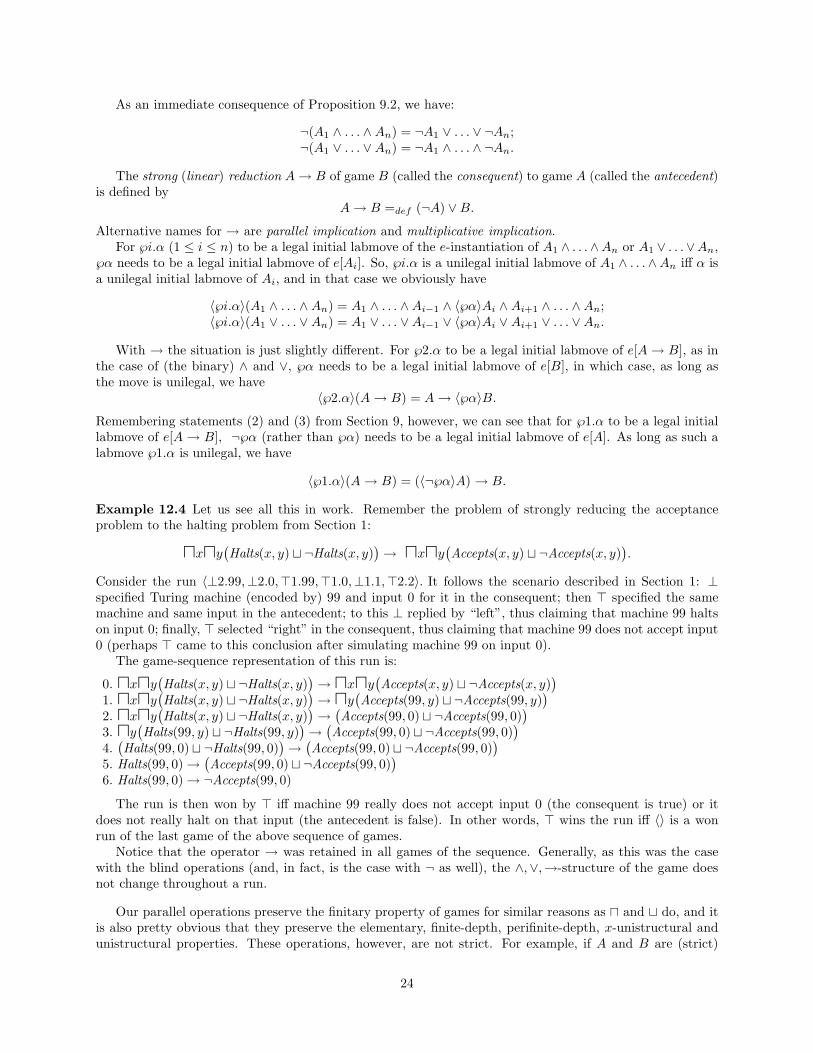
As an immediate consequence of Proposition 9.2, we have:

¬(A1 ∧ . . . ∧ An) = ¬A1 ∨ . . . ∨ ¬An;¬(A1 ∨ . . . ∨ An) = ¬A1 ∧ . . . ∧ ¬An.

The strong (linear) reduction A → B of game B (called the consequent) to game A (called the antecedent)is defined by

A → B =def (¬A) ∨ B.

Alternative names for → are parallel implication and multiplicative implication.For ℘i.α (1 ≤ i ≤ n) to be a legal initial labmove of the e-instantiation of A1 ∧ . . .∧An or A1 ∨ . . .∨An,

℘α needs to be a legal initial labmove of e[Ai]. So, ℘i.α is a unilegal initial labmove of A1 ∧ . . .∧An iff α isa unilegal initial labmove of Ai, and in that case we obviously have

〈℘i.α〉(A1 ∧ . . . ∧ An) = A1 ∧ . . . ∧ Ai−1 ∧ 〈℘α〉Ai ∧ Ai+1 ∧ . . . ∧ An;〈℘i.α〉(A1 ∨ . . . ∨ An) = A1 ∨ . . . ∨ Ai−1 ∨ 〈℘α〉Ai ∨ Ai+1 ∨ . . . ∨ An.

With → the situation is just slightly different. For ℘2.α to be a legal initial labmove of e[A → B], as inthe case of (the binary) ∧ and ∨, ℘α needs to be a legal initial labmove of e[B], in which case, as long asthe move is unilegal, we have

〈℘2.α〉(A → B) = A → 〈℘α〉B.

Remembering statements (2) and (3) from Section 9, however, we can see that for ℘1.α to be a legal initiallabmove of e[A → B], ¬℘α (rather than ℘α) needs to be a legal initial labmove of e[A]. As long as such alabmove ℘1.α is unilegal, we have

〈℘1.α〉(A → B) = (〈¬℘α〉A) → B.

Example 12.4 Let us see all this in work. Remember the problem of strongly reducing the acceptanceproblem to the halting problem from Section 1:

uxuy(Halts(x, y) t ¬Halts(x, y)

)→ uxuy

(Accepts(x, y) t ¬Accepts(x, y)

).

Consider the run 〈⊥2.99,⊥2.0,>1.99,>1.0,⊥1.1,>2.2〉. It follows the scenario described in Section 1: ⊥specified Turing machine (encoded by) 99 and input 0 for it in the consequent; then > specified the samemachine and same input in the antecedent; to this ⊥ replied by “left”, thus claiming that machine 99 haltson input 0; finally, > selected “right” in the consequent, thus claiming that machine 99 does not accept input0 (perhaps > came to this conclusion after simulating machine 99 on input 0).

The game-sequence representation of this run is:

0. uxuy(Halts(x, y) t ¬Halts(x, y)

)→uxuy

(Accepts(x, y) t ¬Accepts(x, y)

)

1. uxuy(Halts(x, y) t ¬Halts(x, y)

)→uy

(Accepts(99, y) t ¬Accepts(99, y)

)

2. uxuy(Halts(x, y) t ¬Halts(x, y)

)→

(Accepts(99, 0) t ¬Accepts(99, 0)

)

3. uy(Halts(99, y) t ¬Halts(99, y)

)→

(Accepts(99, 0) t ¬Accepts(99, 0)

)

4.(Halts(99, 0) t ¬Halts(99, 0)

)→

(Accepts(99, 0) t ¬Accepts(99, 0)

)

5. Halts(99, 0) →(Accepts(99, 0) t ¬Accepts(99, 0)

)

6. Halts(99, 0) → ¬Accepts(99, 0)

The run is then won by > iff machine 99 really does not accept input 0 (the consequent is true) or itdoes not really halt on that input (the antecedent is false). In other words, > wins the run iff 〈〉 is a wonrun of the last game of the above sequence of games.

Notice that the operator → was retained in all games of the sequence. Generally, as this was the casewith the blind operations (and, in fact, is the case with ¬ as well), the ∧,∨,→-structure of the game doesnot change throughout a run.

Our parallel operations preserve the finitary property of games for similar reasons as u and t do, and itis also pretty obvious that they preserve the elementary, finite-depth, perifinite-depth, x-unistructural andunistructural properties. These operations, however, are not strict. For example, if A and B are (strict)

24

games whose only nonempty legal runs are 〈>0〉 and 〈⊥0〉, respectively, then, in the initial position 〈〉 ofA ∧ B, > has the legal move 1.0 and ⊥ has the legal move 2.0. Finally, as all the other game operationsintroduced in this paper, the parallel operations are static. To prove this, we need the following lemma:

Lemma 12.5 Assume A1, . . . , An are static games, ∆ is a ℘-delay of Γ, and ∆ is a ℘-illegal run of e[A1 ∧. . . ∧ An]. Then Γ is also a ℘-illegal run of e[A1 ∧ . . . ∧ An].

Proof. We will prove this lemma by induction on the length of the shortest illegal initial segment of ∆. Tosave space and without loss of generality, we assume that n = 2. For the same reason, we fix an arbitraryvaluation e throughout the context and no longer explicitly mention it.

Assume the conditions of the lemma. We want to show that Γ is a ℘-illegal run of A1 ∧A2. Let 〈Ψ, ℘α〉be the shortest (℘-) illegal initial segment of ∆. Let 〈Φ, ℘α〉 be the shortest initial segment of Γ containingall the ℘-labeled moves7 of 〈Ψ, ℘α〉. If Φ is a ℘-illegal position of A1 ∧ A2, then so is Γ and we are done.Therefore, for the rest of the proof, we assume that

Φ is not a ℘-illegal position of A1 ∧ A2. (11)

Let Θ be the sequence of those ¬℘-labeled moves of Ψ that are not in Φ. Obviously

〈Ψ, ℘α〉 is a ℘-delay of 〈Φ, ℘α, Θ〉. (12)

We also claim thatΦ is a legal position of A1 ∧ A2. (13)

Indeed, suppose this was not the case. Then, by (11), Φ should be ¬℘-illegal. This would make Γ a ¬℘-illegalrun of A1 ∧ A2 with Φ as an illegal initial segment which is shorter than 〈Ψ, ℘α〉. Then, by the inductionhypothesis, any run for which Γ is a ¬℘-delay, would be ¬℘-illegal. But by Lemma 4.6, Γ is a ¬℘-delay of∆. So, ∆ would be ¬℘-illegal, which is a contradiction because, according to our assumption, ∆ is ℘-illegal.

We are continuing our proof. There are two possible reasons to why 〈Ψ, ℘α〉 is an illegal (while Ψ beinglegal) position of A1 ∧ A2:

Reason 1: α does not have the form 1.β or 2.β. Then, in view of (13), 〈Φ, ℘α〉 is a ℘-illegal position ofA1 ∧ A2. As 〈Φ, ℘α〉 happens to be an initial segment of Γ, the latter then is a ℘-illegal run of A1 ∧ A2.

Reason 2: α = i.β (i ∈ {1, 2}) and β 6∈ Lm℘Ai〈Ψi.〉. That is, 〈Ψ, ℘α〉i. is a ℘-illegal position of Ai. (12)obviously implies that 〈Ψ, ℘α〉i. is a ℘-delay of 〈Φ, ℘α, Θ〉i.. Therefore, since Ai is static, Lemma 4.7.1 yieldsthat 〈Φ, ℘α, Θ〉i. is a ℘-illegal position of Ai. Notice that 〈Φ, ℘α, Θ〉i. = 〈Φi., ℘β, Θi.〉. A ℘-illegal positionwill remain ℘-illegal after removing a block of ¬℘-labeled moves (in particular, Θi.) at the end of it. Hence,〈Φi., ℘β〉 is a ℘-illegal position of Ai. In view of (13), this implies that α = i.β 6∈ Lm℘A1∧A2〈Φ〉, so that〈Φ, ℘α〉 is a ℘-illegal position of A1 ∧ A2, and then so is Γ because 〈Φ, ℘α〉 is an initial segment of it. 2

Proposition 12.6 The operations ∧,∨,→ are static.

Proof. As ∨ and → are expressible in terms of ∧ and ¬ and we know that ¬ is static, it will be sufficientto verify that ∧ is static. Also, considering the binary version of ∧ should be sufficient as generalizing fromthe binary to an n-ary case is a straightforward job.

Assume that A1 and A2 are static games, WnA1∧A2e 〈Γ〉 = ℘ and ∆ is a ℘-delay of Γ. Our goal is to show

that WnA1∧A2e 〈∆〉 = ℘.

If ∆ is a ¬℘-illegal run of e[A1 ∧ A2], then it is won by ℘ and we are done. So, assume that ∆ isnot ¬℘-illegal. Then, by Lemmas 4.6 and 12.5, Γ is not ¬℘-illegal, either. Γ also cannot be ℘-illegal, forotherwise it would not be won by ℘. Consequently, ∆ cannot be ℘-illegal either, for otherwise, by Lemma12.5, Γ would be ℘-illegal. Thus, we have narrowed down our considerations to the case when both Γ and∆ are legal runs of e[A1 ∧ A2].

WnA1∧A2e 〈Γ〉 = ℘, together with Γ ∈ LrA1∧A2

e , implies that for both of the i ∈ {1, 2} (if ℘ = >) or one ofthe i ∈ {1, 2} (if ℘ = ⊥), we have that Γi. is a ℘-won run of e[Ai]. Taking into account that ∆i. is obviously

7In this context, different occurrences of the same labmove count as different labmoves. So, a more accurate phrasing wouldbe “as many ℘-labeled moves as...” instead “all the ℘-labeled moves of ...”.

25

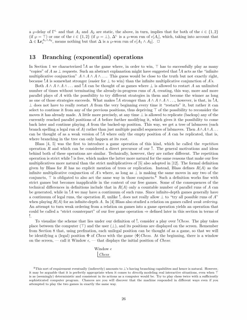
a ℘-delay of Γi. and that A1 and A2 are static, the above, in turn, implies that for both of the i ∈ {1, 2}(if ℘ = >) or one of the i ∈ {1, 2} (if ℘ = ⊥), ∆i. is a ℘-won run of e[Ai], which, taking into account that∆ ∈ LrA1∧A2

e , means nothing but that ∆ is a ℘-won run of e[A1 ∧ A2]. 2

13 Branching (exponential) operations

In Section 1 we characterized !A as the game where, in order to win, > has to successfully play as many“copies” of A as ⊥ requests. Such an abstract explanation might have suggested that !A acts as the “infinitemultiplicative conjunction” A ∧ A ∧ A ∧ . . .. This guess would be close to the truth but not exactly right,because !A is somewhat stronger (easier for ⊥ to win) than the infinite multiplicative conjunction of A’s.

Both A ∧ A ∧ A ∧ . . . and !A can be thought of as games where ⊥ is allowed to restart A an unlimitednumber of times without terminating the already-in-progress runs of A, creating, this way, more and moreparallel plays of A with the possibility to try different strategies in them and become the winner as longas one of those strategies succeeds. What makes !A stronger than A ∧ A ∧ A ∧ . . ., however, is that, in !A,⊥ does not have to really restart A from the very beginning every time it “restarts” it, but rather it canselect to continue it from any of the previous positions, thus depriving > of the possibility to reconsider themoves it has already made. A little more precisely, at any time ⊥ is allowed to replicate (backup) any of thecurrently reached parallel positions of A before further modifying it, which gives it the possibility to comeback later and continue playing A from the backed-up position. This way, we get a tree of labmoves (eachbranch spelling a legal run of A) rather than just multiple parallel sequences of labmoves. Then A∧A∧A . . .can be thought of as a weak version of !A where only the empty position of A can be replicated, that is,where branching in the tree can only happen at its root.

Blass [4, 5] was the first to introduce a game operation of this kind, which he called the repetitionoperation R and which can be considered a direct precursor of our !. The general motivations and ideasbehind both of these operations are similar. Technically, however, they are rather different. The repetitionoperation is strict while ! is free, which makes the latter more natural for the same reasons that make our freemultiplicatives more natural than the strict multiplicatives of [5] also adopted in [12]. The formal definitiongiven by Blass for R has no explicit mention of trees or replication. Instead, Blass defines R(A) as theinfinite multiplicative conjunction of A’s where, as long as ⊥ is making the same moves in any two of theconjuncts, > is obligated to also act the same way in those conjuncts.8 Such a definition works fine withstrict games but becomes inapplicable in the context of our free games. Some of the consequences of thetechnical differences in definitions include that in R(A) only a countable number of parallel runs of A canbe generated, while in !A we may have a continuum of such runs. Since infinite-depth games generally havea continuum of legal runs, the operation R, unlike !, does not really allow ⊥ to “try all possible runs of A”when playing R(A) for an infinite-depth A. In [4] Blass also studied a relation on games called weak ordering.An attempt to turn weak ordering from a relation on games into a game operation yields an operation thatcould be called a “strict counterpart” of our free game operation ⇒ defined later in this section in terms of!.

To visualize the scheme that lies under our definition of !, consider a play over !Chess. The play takesplace between the computer (>) and the user (⊥), and its positions are displayed on the screen. Rememberfrom Section 8 that, using prefixation, each unilegal position can be thought of as a game, so that we willbe identifying a (legal) position Φ of Chess with the game 〈Φ〉Chess. At the beginning, there is a windowon the screen, — call it Window ε, — that displays the initial position of Chess:

Window ε

Chess

8This sort of requirement eventually (indirectly) amounts to ⊥’s having branching capabilites and hence is natural. However,it may be arguable that it is perfectly appropriate when it comes to directly modeling real interactive situations, even when >is as (seemingly) deterministic and consistent in its actions as a computer would be. Try to play chess twice with a sufficientlysophisticated computer program. Chances are you will discover that the machine responded in different ways even if youattempted to play the two games in exactly the same way.

26

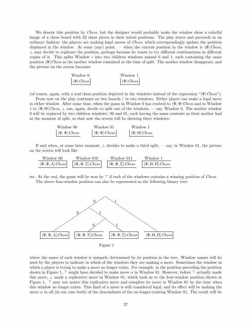
We denote this position by Chess, but the designer would probably make the window show a colorfulimage of a chess board with 32 chess pieces in their initial positions. The play starts and proceeds in anordinary fashion: the players are making legal moves of Chess, which correspondingly update the positiondisplayed in the window. At some (any) point, — when the current position in the window is 〈Φ〉Chess,⊥ may decide to replicate the position, perhaps because he wants to try different continuations in differentcopies of it. This splits Window ε into two children windows named 0 and 1, each containing the sameposition 〈Φ〉Chess as the mother window contained at the time of split. The mother window disappears, andthe picture on the screen becomes

Window 1〈Φ〉Chess

Window 0〈Φ〉Chess

(of course, again, with a real chess position depicted in the windows instead of the expression “〈Φ〉Chess”).From now on the play continues on two boards / in two windows. Either player can make a legal move

in either window. After some time, when the game in Window 0 has evolved to 〈Φ, Ψ〉Chess and in Window1 to 〈Φ, Θ〉Chess, ⊥ can, again, decide to split one of the windows, — say, Window 0. The mother window0 will be replaced by two children windows: 00 and 01, each having the same contents as their mother hadat the moment of split, so that now the screen will be showing three windows:

Window 1〈Φ, Θ〉Chess

Window 00〈Φ, Ψ〉Chess

Window 01〈Φ, Ψ〉Chess

If and when, at some later moment, ⊥ decides to make a third split, — say, in Window 01, the pictureon the screen will look like

Window 1〈Φ, Θ, Π〉Chess

Window 00〈Φ, Ψ, Λ〉Chess

Window 010〈Φ, Ψ, Σ〉Chess

Window 011〈Φ, Ψ, Σ〉Chess

etc. At the end, the game will be won by > if each of the windows contains a winning position of Chess.The above four-window position can also be represented as the following binary tree:

〈Φ, Θ, Π〉Chess〈Φ, Ψ, Λ〉Chess 〈Φ, Ψ, Σ〉Chess 〈Φ, Ψ, Σ〉Chess

Figure 1

QQ

QQ

QQ

QQ

QQ

QQQ

��

��

��

��

��

���

QQ

QQ

ZZ

ZZZ

��

���

0 1

0 1

0 1

where the name of each window is uniquely determined by its position in the tree. Window names will beused by the players to indicate in which of the windows they are making a move. Sometimes the window inwhich a player is trying to make a move no longer exists. For example, in the position preceding the positionshown in Figure 1, > might have decided to make move α in Window 01. However, before > actually madethis move, ⊥ made a replicative move in Window 01, which took us to the four-window position shown inFigure 1. > may not notice this replicative move and complete its move in Window 01 by the time whenthis window no longer exists. This kind of a move is still considered legal, and its effect will be making themove α in all (in our case both) of the descendants of the no-longer-existing Window 01. The result will be

27

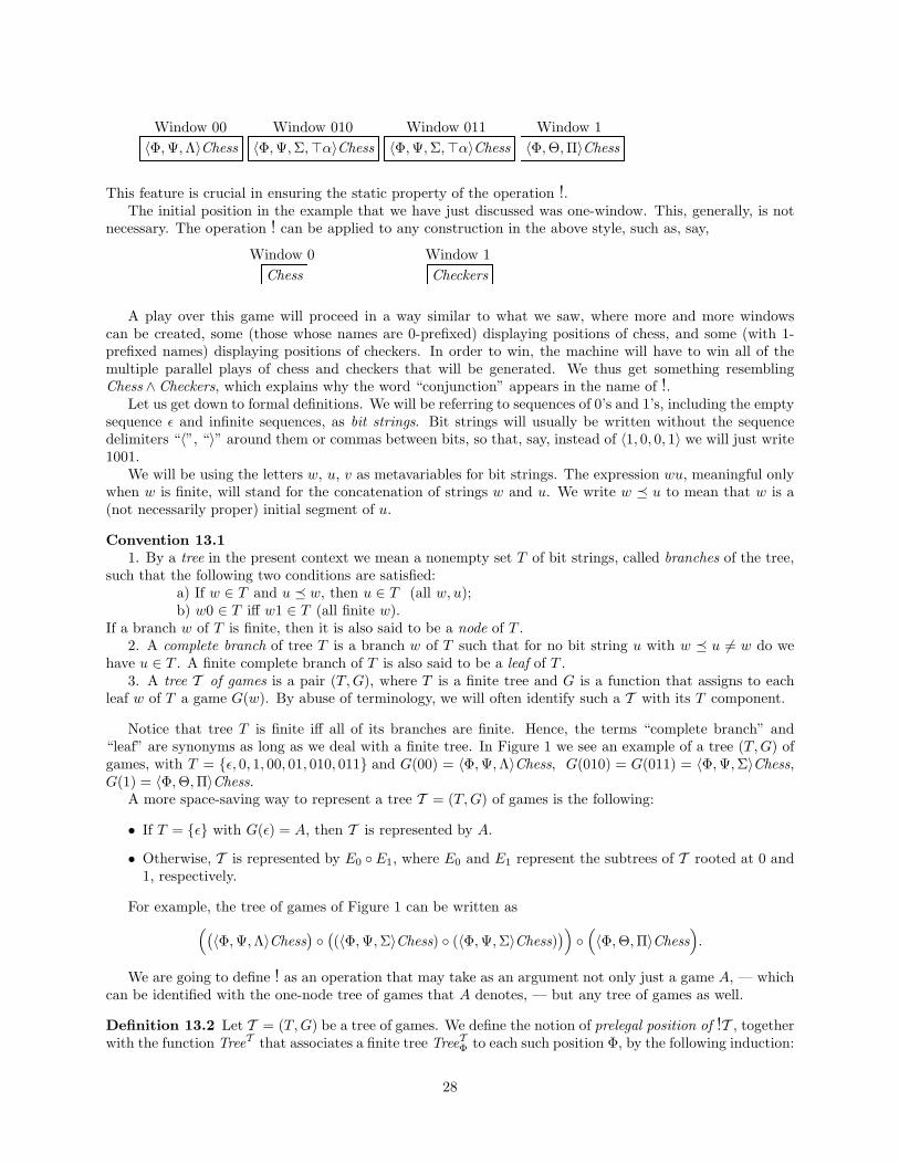
Window 1〈Φ, Θ, Π〉Chess

Window 00〈Φ, Ψ, Λ〉Chess

Window 010〈Φ, Ψ, Σ,>α〉Chess

Window 011〈Φ, Ψ, Σ,>α〉Chess

This feature is crucial in ensuring the static property of the operation !.The initial position in the example that we have just discussed was one-window. This, generally, is not

necessary. The operation ! can be applied to any construction in the above style, such as, say,

Window 1Checkers

Window 0Chess

A play over this game will proceed in a way similar to what we saw, where more and more windowscan be created, some (those whose names are 0-prefixed) displaying positions of chess, and some (with 1-prefixed names) displaying positions of checkers. In order to win, the machine will have to win all of themultiple parallel plays of chess and checkers that will be generated. We thus get something resemblingChess ∧ Checkers, which explains why the word “conjunction” appears in the name of !.

Let us get down to formal definitions. We will be referring to sequences of 0’s and 1’s, including the emptysequence ε and infinite sequences, as bit strings. Bit strings will usually be written without the sequencedelimiters “〈”, “〉” around them or commas between bits, so that, say, instead of 〈1, 0, 0, 1〉 we will just write1001.

We will be using the letters w, u, v as metavariables for bit strings. The expression wu, meaningful onlywhen w is finite, will stand for the concatenation of strings w and u. We write w � u to mean that w is a(not necessarily proper) initial segment of u.

Convention 13.11. By a tree in the present context we mean a nonempty set T of bit strings, called branches of the tree,

such that the following two conditions are satisfied:a) If w ∈ T and u � w, then u ∈ T (all w, u);b) w0 ∈ T iff w1 ∈ T (all finite w).

If a branch w of T is finite, then it is also said to be a node of T .2. A complete branch of tree T is a branch w of T such that for no bit string u with w � u 6= w do we

have u ∈ T . A finite complete branch of T is also said to be a leaf of T .3. A tree T of games is a pair (T, G), where T is a finite tree and G is a function that assigns to each

leaf w of T a game G(w). By abuse of terminology, we will often identify such a T with its T component.

Notice that tree T is finite iff all of its branches are finite. Hence, the terms “complete branch” and“leaf” are synonyms as long as we deal with a finite tree. In Figure 1 we see an example of a tree (T, G) ofgames, with T = {ε, 0, 1, 00, 01, 010, 011} and G(00) = 〈Φ, Ψ, Λ〉Chess, G(010) = G(011) = 〈Φ, Ψ, Σ〉Chess,G(1) = 〈Φ, Θ, Π〉Chess.

A more space-saving way to represent a tree T = (T, G) of games is the following:

• If T = {ε} with G(ε) = A, then T is represented by A.

• Otherwise, T is represented by E0 ◦E1, where E0 and E1 represent the subtrees of T rooted at 0 and1, respectively.

For example, the tree of games of Figure 1 can be written as((

〈Φ, Ψ, Λ〉Chess)◦

((〈Φ, Ψ, Σ〉Chess) ◦ (〈Φ, Ψ, Σ〉Chess)

))◦

(〈Φ, Θ, Π〉Chess

).

We are going to define ! as an operation that may take as an argument not only just a game A, — whichcan be identified with the one-node tree of games that A denotes, — but any tree of games as well.

Definition 13.2 Let T = (T, G) be a tree of games. We define the notion of prelegal position of !T , togetherwith the function TreeT that associates a finite tree TreeTΦ to each such position Φ, by the following induction:

28

1. 〈〉 is a prelegal position of !T , and TreeT〈〉 = T .

2. 〈Φ, λ〉 is a prelegal position of !T iff Φ is so and one of the following two conditions is satisfied:

(a) λ = ⊥w: for some leaf w of TreeTΦ . We call this sort of a labmove λ a replicative labmove. In thiscase TreeT〈Φ,λ〉 = TreeTΦ ∪ {w0, w1}.

(b) λ is ⊥w.α or >w.α for some node w of TreeTΦ and move α. We call this sort of a labmove λ anonreplicative labmove. In this case TreeT〈Φ,λ〉 = TreeTΦ .

The terms “replicative” and “nonreplicative” will also be extended from labmoves to moves.

Intuitively, TreeTΦ is the tree, in the style of Figure 1, that will be seen on the screen after the sequenceΦ of labmoves has been made when playing the game !T ; TreeTΦ only describes the tree-structure of theposition represented on the screen, without showing the contents of its windows. Therefore, whether Φ is aprelegal position of !T and what the value of TreeTΦ is, only depends on the T component of T and does notdepend on its G component.

The meaning of a replicative labmove ⊥w: is that ⊥ replicates (splits) window w; the meaning of anonreplicative labmove ℘w.α is that player ℘ makes the move α in all windows whose names start with w.

The concept of prelegal position of !T can be generalized to all runs by stipulating that a prelegal run of!T is a run whose every finite initial segment is a prelegal position of !T . Similarly, the function TreeT canbe extended to all prelegal runs of !T by stipulating that

TreeT〈λ1,λ2,λ3,...〉 = TreeT〈〉 ∪ TreeT〈λ1〉 ∪ TreeT〈λ1,λ2〉 ∪ TreeT〈λ1,λ2,λ3〉 ∪ . . .

Convention 13.3 Let u be a bit string and Γ any run. Then Γ�u will stand for the result of first removingfrom Γ all the labmoves except those that look like ℘w.α for some bit string w with w � u, and then deletingthis sort of prefixes “w.” in the remaining labmoves, i.e. replacing each remaining labmove ℘w.α (where wis a bit string) by ℘α.

Example: If u = 101000 . . . and Γ = 〈>.α1,⊥:,⊥1.α2,>0.α3,⊥1:,>10.α4〉, then Γ�u = 〈>α1,⊥α2,>α4〉.

Being a prelegal run of !T is a necessary but not a sufficient condition for being a legal run of this game.For simplicity, let us consider the case when T is a one-node tree A of games. It was mentioned at thebeginning of this section that a legal run Γ of !A can be thought of as consisting of multiple parallel legalruns of A. In particular, these runs will be the runs Γ�u, where u is a complete branch of TreeA

Γ . Thelabmoves of Γ�u for such a u are those ℘α that emerged as a result of making (nonreplicative) labmoves ofthe form ℘w.α with w � u. For example, to the branch 010 in Figure 1 corresponds the run 〈Φ, Ψ, Σ〉, wherethe labmoves of Φ originate from the nonreplicative labmoves of the form ℘ε.α (i.e. ℘.α) made before thefirst replicative move, the labmoves of Ψ originate from the nonreplicative labmoves of the form ℘w.α withw � 0 made between the first and the second replicative moves, and the labmoves of Σ originate from thenonreplicative labmoves of the form ℘w.α with w � 01 made between the second and the third replicativemoves. Generally, for a prelegal run Γ of !A to be a legal run, it is necessary and sufficient that all of theruns Γ�u, where u is a complete branch of TreeA

Γ , be legal runs of A. And for such a Γ to be a >-won run, itis necessary and sufficient that all of those Γ�u be >-won runs of A. In fact, the meaning of what we havejust said will not change if we let u range over all infinite bit strings rather than all complete branches ofTreeA

Γ . Indeed, if u is a finite complete branch (i.e. leaf) of TreeAΓ , for any w we obviously have Γ�u = Γ�uw,

so that it does not matter whether we talk about u or any of its infinite extensions uw. And vice versa: ifan infinite bit string u does not happen to be a complete branch of TreeA

Γ , in view of Convention 13.1.1b, itis clear that the shortest initial segment v of u that is a node of TreeA

Γ will be a complete branch (leaf) ofTreeA

Γ , so that, again because Γ�u = Γ�v, it does not matter whether we talk about u or v.When T is a multiple-node tree of games, the situation is similar. For example, for Γ to be a legal (resp.

>-won) run of !(Chess ◦Checkers), along with being a prelegal run, it is necessary that, for every infinite bitstring 0u, Γ�0u be a legal (resp. >-won) run of Chess and, for every infinite bit string 1u, Γ�1u be a legal(resp. >-won) run of Checkers.

This intuition is summarized below in our formal definition of !.

29

Definition 13.4 Suppose T = (T, G) is a tree of games. The branching (exponential) conjunction !T of Tis defined as follows:

1. Γ ∈ Lr!Te iff the following two conditions are satisfied:

(a) Γ is a prelegal run of !T .(b) For every infinite bit string wu where w is a leaf of T , Γ�wu ∈ LrG(w)

e .2. As long as Γ ∈ Lr!T

e , Wn!Te 〈Γ〉 = > iff WnG(w)

e 〈Γ�wu〉 = > for every infinite bit string wu where w isa leaf of T .

As always, we want to have an inductive characterization (see page 19) of the game operation we havejust introduced. The initial conditions are pretty obvious:

Proposition 13.5 Let T = (T, G) be a tree of games. Then:

1. λ is a legal initial labmove of !T w.r.t. e iff one of the following conditions is satisfied:

(a) λ is the (replicative) labmove ⊥w: for some leaf w of T .

(b) λ is the (nonreplicative) labmove ℘w.α for some node w of T and move α such that α ∈ Lm℘G(u)e 〈〉

for every leaf u of T with w � u.

2. Wn!Te 〈〉 = > iff, for each leaf w of T , WnG(w)

e 〈〉 = >.

For the inductive clause (Proposition 13.8), we need the following two definitions.

Definition 13.6 Let T = (T, G) be a tree of games and w a leaf of T . We define Repw[T ] as the followingtree (T ′, G′) of games:

1. T ′ = T ∪ {w0, w1}2. (a) G′(w0) = G′(w1) = G(w)

(b) For every other (different from w0, w1) leaf u of T ′, G′(u) = G(u).

Example: Rep10[A ◦ (B ◦ C)] = A ◦((B ◦ B) ◦ C

).

Definition 13.7 Suppose T = (T, G) is a tree of games, w is a node of T and, for every leaf u of T withw � u, λ is a unilegal initial labmove of G(u). We define Nonrepλ

w[T ] as the tree (T, G′) of games such that:1. For every leaf u of T with w � u, G′(u) = 〈λ〉G(u).2. For every other leaf u of T , G′(u) = G(u).

Example: Nonrepλ1 [A ◦ (B ◦ C)] = A ◦ (〈λ〉B ◦ 〈λ〉C) (any λ that is a unilegal initial labmove of both

B and C).

Proposition 13.8 Suppose T is a tree of games, and λ is a unilegal initial labmove of !T .1. If λ is a replicative labmove ⊥w:, then 〈λ〉!T = !Repw[T ].2. If λ is a nonreplicative labmove ℘w.α, then 〈λ〉!T = !Nonrep℘α

w [T ].

We postpone the proof of this fact till the end of the section. As for now, let us see an application of theabove inductive characterization of !.

Example 13.9 In view of Propositions 13.5 (initial conditions) and 13.8 (inductive clause), the sequence〈⊥:,⊥0.4,>0.16,⊥1:,⊥10.5,>10.25〉 is a unilegal, >-won run of the game !uxty(y = x2), and the game-sequence representation of this run is:0. !

(uxty(y = x2)

)

1. !(uxty(y = x2) ◦uxty(y = x2)

)

2. !(ty(y = 42) ◦uxty(y = x2)

)

3. !((16 = 42) ◦uxty(y = x2)

)

4. !((16 = 42) ◦

(uxty(y = x2) ◦uxty(y = x2)))

5. !((16 = 42) ◦

(ty(y = 52) ◦uxty(y = x2)))

6. !((16 = 42) ◦

((25 = 52) ◦uxty(y = x2)

))

30

Every version of conjunction has its dual disjunction, and so does !. For a tree T = (T, G) of games, let ¬Tmean the tree (T, G′) of games where, for each leaf w of T , G′(w) = ¬G(w). Then we define the branching(exponential) disjunction ?T of T by

?T =def ¬!¬T .

As we may guess, the meaning of ?T is the same as that of !T , only with the roles of the two playersinterchanged: in a ?-game, it is > rather than ⊥ who can replicate positions, and, in order to win, it issufficient for > to win in at least one rather than all of the parallel runs that will be created during the play.

Remembering that a game is nothing but a one-node tree of games, from now on we will usually treat! and ? as game operations rather than (the more general) operations on trees of games. The only reasonwhy we originally defined them as operations on trees of games was to make inductive characterizations andhence visualizations in the style of Example 13.9 possible.

The weak reduction A ⇒ B of game B (called the consequent) to game A (called the antecedent) is definedby

A ⇒ B =def (!A) → B.

Alternative names for ⇒ are branching implication and exponential implication. We saw an informal de-scription of a play over a ⇒-game in Section 1 when discussing the intuitive meaning of weak reduction.

For both ! and ? we can define their bounded versions !b and ?b, where b is a positive integer. Themeanings of !bA and ?b

A are the same as those of !A and ?A, with the only difference that the numberof parallel plays of A that the corresponding player can create should not exceed b, that is, at most b − 1replicative moves can be made legally.

As an exercise showing the essential difference between branching and parallel operations (somethingthat Example 13.9 fails to really demonstrate), the reader may want to compare the games ?2

D and D∨D,where

D = (Chess t ¬Chess) u (Checkers t ¬Checkers).

Which of the two games is easier for > to win?It is evident that the operations !, ?,⇒, being similar to the parallel operations, are not strict. Nor are

they elementary, for replicative moves, even though pointless, would still be legal in !A with an elementaryA, so that !A would not even be perifinite-depth, let alone elementary. So, the branching operations are notfinite- or perifinite-depth, either. It is left as an exercise for the reader to verify that ! (and hence ? and ⇒)are finitary, unistructural and x-unistructural. Finally, like all the other game operations that we have seen,the branching operations are static. To prove this, we need the following lemma:

Lemma 13.10 Assume A is a static game, ∆ is a ℘-delay of Γ, and ∆ is a ℘-illegal run of e[!A]. Then Γis also a ℘-illegal run of e[!A].

Proof. Assume the conditions of the lemma. Valuation e will be fixed throughout the context and doesnot need to be explicitly mentioned. We want to show that Γ is a ℘-illegal run of !A.

Let 〈Ψ, ℘α〉 be the shortest initial segment of ∆ that is a ℘-illegal position of !A. Let 〈Φ, ℘α〉 be theshortest initial segment of Γ containing all the ℘-labeled moves of 〈Ψ, ℘α〉, and let Θ be the sequence ofthose ¬℘-labeled moves of Ψ that are not in Φ, so that we obviously have

〈Ψ, ℘α〉 is a ℘-delay of 〈Φ, ℘α, Θ〉. (14)

Excluding from our considerations the trivial case when Φ is a ℘-illegal position of !A and reasoningexactly as in the proof of Lemma 12.5, the following statement can be shown to be true:

Φ is a legal position of !A. (15)

There are two possible reasons to why 〈Ψ, ℘α〉 is a ℘-illegal (while Ψ being legal) position of !A:Reason 1: 〈Ψ, ℘α〉 is not a prelegal position of !A. We claim that then 〈Φ, ℘α〉 is not a prelegal position

of !A which, in view of (15), implies that 〈Φ, ℘α〉 and hence its extension Γ is a ℘-illegal run of !A. To provethis claim, suppose, for a contradiction, that 〈Φ, ℘α〉 is a prelegal position of !A. Note that TreeA

Ψ and TreeAΦ

31

(Definition 13.2) are both defined because both Ψ and Φ are legal (Ψ by our original assumption and Φ by(15)) and hence prelegal positions of !A. There are two cases to consider:

Case 1: ℘ = ⊥. Note that then Φ and Ψ have the same subsequences of ⊥-labeled moves and hence (asall replicative moves are ⊥-labeled) the same subsequences of replicative labmoves. From Definition 13.2then it is obvious that TreeA

Ψ = TreeAΦ . This is so because TreeA is modified, — in particular, extended, —

only by replicative moves. Then we immediately get that 〈Ψ, ℘α〉 is a prelegal position of !A if and only if〈Φ, ℘α〉 is so, which is a contradiction.

Case 2: ℘ = >. This means that α = w.β for some w ∈ TreeAΦ . Note that, since ℘ = >, the subsequence

of ⊥-labeled moves of Φ is an initial segment of that of Ψ, so that the subsequence of replicative labmovesof Φ is an initial segment of that of Ψ. This obviously implies that TreeA

Φ ⊆ TreeAΨ, from which we can

conclude that w ∈ TreeAΨ and hence 〈Ψ,>w.β〉, i.e. 〈Ψ, ℘α〉, is a prelegal position of !A, which, again, is a

contradiction.Reason 2: There is an infinite bit string u such that 〈Ψ, ℘α〉�u is not a legal position of A. Since Ψ,

by our original assumption, is a legal position of !A, Ψ�u must be a legal position of A. Hence, 〈Ψ, ℘α〉�u

is a ℘-illegal position of A. From (14) we can see that 〈Ψ, ℘α〉�u is a ℘-delay of 〈Φ, ℘α, Θ〉�u. Therefore,taking into account that A is static, Lemma 4.7.1 implies that 〈Φ, ℘α, Θ〉�u is a ℘-illegal position of A. Then〈Φ, ℘α〉�u is also a ℘-illegal position of A, because all the moves of Θ are ¬℘-labeled. This makes 〈Φ, ℘α〉and hence its extension Γ a ℘-illegal run of !A. 2

Proposition 13.11 The operations !, ? and ⇒ are static.

Proof. As always, it will be sufficient to prove the proposition for only the basic operation of the group,in particular, !. It should be pointed out that the proof we give below can be easily converted into a proofof the fact that the operation !, applied to any tree of static games rather than a single-node tree A, alsoyields a static game.

Assume A is a static game, ∆ is a ℘-delay of Γ, and Wn!Ae 〈Γ〉 = ℘. We need to show that Wn!A

e 〈∆〉 = ℘.If ∆ is a ¬℘-illegal run of e[!A], then it is won by ℘ and we are done. So, assume that ∆ is not ¬℘-illegal.

Then, by Lemmas 4.6 and 13.10, Γ is not ¬℘-illegal, either. Γ also cannot be ℘-illegal, for otherwise it wouldnot be won by ℘. Consequently, ∆ cannot be ℘-illegal either, for otherwise, by Lemma 13.10, Γ would be℘-illegal. Thus, we have narrowed down our considerations to the case when both Γ and ∆ are legal runs ofe[!A].

Wn!Ae 〈Γ〉 = ℘, together with Γ ∈ Lr!A

e , implies that for each infinite bit string u (if ℘ = >), or one ofsuch strings u (if ℘ = ⊥), Γ�u is a ℘-won run of e[A]. Taking into account that ∆�u is obviously a ℘-delayof Γ�u and that A is static, the above, in turn, implies that for each infinite bit string u (if ℘ = >), or oneof such strings u (if ℘ = ⊥), ∆�u is a ℘-won run of e[A], which, taking into account that ∆ ∈ Lr!A

e , meansnothing but that ∆ is a ℘-won run of e[!A]. 2

Our remaining duty is to prove Proposition 13.8, to which the rest of this section is devoted. The readerwho has no reasons to doubt the correctness of that proposition, may safely skip this part.

Proof of Proposition 13.8, Clause 1. Assume T = (T, G) and ⊥w: is a unilegal initial (replicative)labmove of !T . Let us fix the tree T ′ = (T ′, G′) of games with T ′ = Repw[T ]. Our goal is to show that boththe Lr and the Wn components of the games !T ′ and 〈⊥w:〉!T are the same.

At first, we claim that, for any Φ,

Φ is a prelegal position of !T ′ iff 〈⊥w:, Φ〉 is a prelegal position of !T . (16)

This claim can be verified by induction on the length of Φ, showing, in parallel, that when 〈⊥w:, Φ〉 is aprelegal position of !T (and hence Φ a prelegal position of !T ′), TreeT

′

Φ = TreeT〈⊥w:,Φ〉. We omit here thisstraightforward induction which is based on a simple analysis of Definition 13.2.

Consider an arbitrary position Φ. We want to show that Φ 6∈ Lr〈⊥w:〉!Te iff Φ 6∈ Lr!T ′

e .Assume Φ 6∈ Lr〈⊥w:〉!T

e , i.e. (by Definition 8.1) 〈⊥w:, Φ〉 6∈ Lr!Te . If the reason for 〈⊥w:, Φ〉 6∈ Lr!T

e isthat 〈⊥w:, Φ〉 is not a prelegal position of !T , then, by (16), Φ is not a prelegal position of !T ′ and henceΦ 6∈ Lr!T ′

e . Suppose now the reason for 〈⊥w:, Φ〉 6∈ Lr!Te is that, for some leaf v of T and some infinite bit

32

string u with v � u, 〈⊥w:, Φ〉�u 6∈ LrG(v)e , i.e., since we clearly have 〈⊥w:, Φ〉�u = Φ�u, Φ�u 6∈ LrG(v)

e . Ifv happens to be a leaf of T ′, then we immediately get Φ 6∈ Lr!T ′

e . Otherwise, we must have v = w. Thenw0 � u or w1 � u. In either case there is a leaf v′ (= w0 or w1) of T ′ such that v′ � u and Φ�u 6∈ LrG(w)

e .But note that, by Definition 13.6.2a, G(w) = G′(v′). Thus, again we get that Φ 6∈ Lr!T ′

e .Now assume Φ 6∈ Lr!T ′

e . If the reason for Φ 6∈ Lr!T ′

e is that Φ is not a prelegal position of !T ′, then, by(16), 〈⊥w:, Φ〉 is not a prelegal position of !T , whence 〈⊥w:, Φ〉 6∈ Lr!T

e , which means that Φ 6∈ Lr〈⊥w:〉!Te .

Suppose now the reason for Φ 6∈ Lr!T ′

e is that, for some leaf v of T ′ and some infinite bit string u with v � u,Φ�u is not a legal position of G′(v) w.r.t. e. If v happens to be a leaf of T , then G′(v) = G(v) and thereforeΦ�u 6∈ LrG(v)

e , i.e. 〈⊥w:, Φ〉�u 6∈ LrG(v)e , whence 〈⊥w:, Φ〉 6∈ Lr!T

e , i.e. Φ 6∈ Lr〈⊥w:〉!Te . Suppose now v is not a

leaf of T . Then v = w0 or v = w1, so that G′(v) = G(w) and hence Φ�u 6∈ LrG(w)e , i.e. 〈⊥w:, Φ〉�u 6∈ LrG(w)

e

which, taking into account that w � u, again implies that 〈⊥w:, Φ〉 6∈ Lr!Te , i.e. Φ 6∈ Lr〈⊥w:〉!T

e .Next, consider an arbitrary run Γ with Γ ∈ Lr!T ′

e = Lr〈⊥w:〉!Te . We want to show that Wn〈⊥w:〉!T

e 〈Γ〉 = ⊥iff Wn!T ′

e 〈Γ〉 = ⊥.Assume Wn〈⊥w:〉!T

e 〈Γ〉 = ⊥, i.e. Wn!Te 〈⊥w:, Γ〉 = ⊥. Then, by Definition 13.4.2, there is a leaf v of T

and an infinite bit string u with v � u such that WnG(v)e 〈⊥w:, Γ〉�u = ⊥, i.e. WnG(v)

e 〈Γ�u〉 = ⊥. If v alsohappens to be a leaf of T ′, then, by Definition 13.6, G′(v) = G(v) and, hence, Wn!T ′

e 〈Γ〉 = ⊥. Otherwise,we have v = w. But then w0 � u or w1 � u and, since w0, w1 are leaves of T ′ and G′(w0) = G′(w1) = G(v),we again have that Wn!T ′

e 〈Γ〉 = ⊥.Now assume that Wn!T ′

e 〈Γ〉 = ⊥. There must be a leaf v of T ′ and an infinite bit string u with v � u

such that WnG′(v)e 〈Γ�u〉 = ⊥. Just as in the previous case, if v also happens to be a leaf of T , we get that

Wn〈⊥w:〉!Te 〈Γ〉 = ⊥. Otherwise, v must be w0 or w1. In either case w � u and WnG(w)

e 〈Γ�u〉 = ⊥, which,again, implies that Wn〈⊥w:〉!T

e 〈Γ〉 = ⊥. 2

Proof of Proposition 13.8, Clause 2. Assume T = (T, G) and ℘w.α is a unilegal initial nonreplicativelabmove of !T . Let us fix the tree T ′ = (T, G′) of games with T ′ = Nonrep℘α

w [T ]. Our goal is to show thatboth the Lr and the Wn components of the games !T ′ and 〈℘w.α〉!T are the same.

Just as in the proof of clause 1 (statement (16)), — in fact, in an even easier way, — we can show that,for any Φ,

Φ is a prelegal position of !T ′ iff 〈℘w.α, Φ〉 is a prelegal position of !T . (17)

Consider an arbitrary position Φ. We want to show that Φ 6∈ Lr〈℘w.α〉!Te iff Φ 6∈ Lr!T ′

e .Assume Φ 6∈ Lr〈℘w.α〉!T

e , i.e. 〈℘w.α, Φ〉 6∈ Lr!Te . If the reason for 〈℘w.α, Φ〉 6∈ Lr!T

e is that 〈℘w.α, Φ〉 isnot a prelegal position of !T , then, by (17), Φ is not a prelegal position of !T ′, which implies that Φ 6∈ Lr!T ′

e .Suppose now the reason for 〈℘w.α, Φ〉 6∈ Lr!T

e is that for some leaf v of T and some infinite bit stringu with v � u, 〈℘w.α, Φ〉�u 6∈ LrG(v)

e . If w 6� v, then G(v) = G′(v) and 〈℘w.α, Φ〉�u = Φ�u, so thatΦ�u 6∈ LrG′(v)

e and hence Φ 6∈ Lr!T ′

e . Suppose now w � v. Notice that then 〈℘w.α, Φ〉�u = 〈℘α, Φ�u〉. So,since 〈℘w.α, Φ〉�u 6∈ LrG(v)

e , we have 〈℘α, Φ�u〉 6∈ LrG(v)e , i.e. Φ�u 6∈ Lr〈℘α〉G(v)

e . But by Definition 13.7.1,〈℘α〉G(v) = G′(v). Hence, Φ�u 6∈ LrG′(v)

e , which means that Φ 6∈ Lr!T ′

e .Now assume Φ 6∈ Lr!T ′

e . If the reason for Φ 6∈ Lr!T ′

e is that Φ is not a prelegal position of !T ′, then, by(17), 〈℘w.α, Φ〉 is not a prelegal position of !T , so that 〈℘w.α, Φ〉 6∈ Lr!T

e , i.e. Φ 6∈ Lr〈℘w.α〉!Te . Suppose

now the reason for Φ 6∈ Lr!T ′

e is that, for some leaf v of T and some infinite bit string u with v � u,Φ�u 6∈ LrG′(v)

e . If w 6� v, then G′(v) = G(v) and Φ�u = 〈℘w.α, Φ〉�u, so that 〈℘w.α, Φ〉�u 6∈ LrG(v)e and

hence 〈℘w.α, Φ〉 6∈ Lr!Te , i.e. Φ 6∈ Lr〈℘w.α〉!T

e . Suppose now w � v. Then 〈℘w.α, Φ〉�u = 〈℘α, Φ�u〉. SinceΦ�u 6∈ LrG′(v)

e and G′(v) = 〈℘α〉G(v), we have that Φ�u 6∈ Lr〈℘α〉G(v)e , i.e. 〈℘α, Φ�u〉 6∈ LrG(v)

e , whence〈℘w.α, Φ〉�u 6∈ LrG(v)

e , which means that 〈℘w.α, Φ〉 6∈ Lr!Te , i.e. Φ 6∈ Lr〈℘w.α〉!T

e .Next, consider an arbitrary run Γ with Γ ∈ Lr!T ′

e = Lr〈℘w.α〉!Te . We want to show that Wn〈℘w.α〉!T

e 〈Γ〉 =⊥ iff Wn!T ′

e 〈Γ〉 = ⊥.Assume Wn〈℘w.α〉!T

e 〈Γ〉 = ⊥, i.e. Wn!Te 〈℘w.α, Γ〉 = ⊥. Then there is a leaf v of T and an infinite bit

string u with v � u such that WnG(v)e 〈℘w.α, Γ〉�u = ⊥. If w 6� v, then G(v) = G′(v) and 〈℘w.α, Γ〉�u = Γ�u,

so that we have WnG′(v)e (Γ�u) = ⊥, which implies Wn!T ′

e 〈Γ〉 = ⊥. Suppose now w � v. Then G′(v) =

33

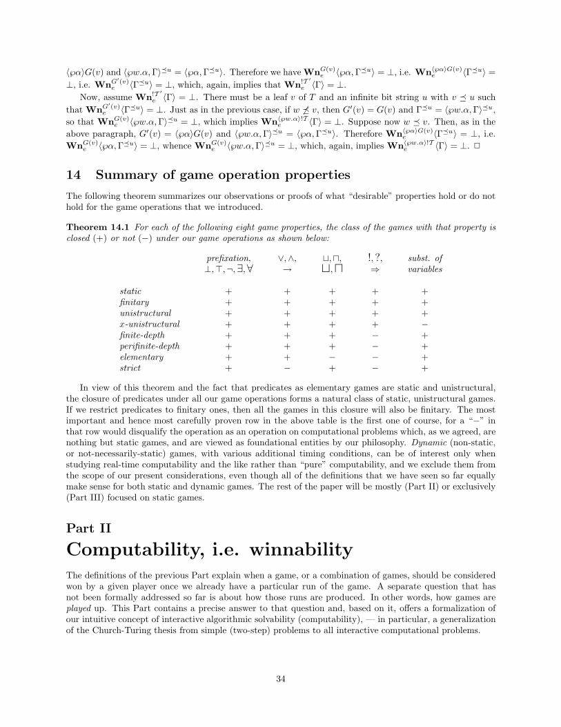
〈℘α〉G(v) and 〈℘w.α, Γ〉�u = 〈℘α, Γ�u〉. Therefore we have WnG(v)e 〈℘α, Γ�u〉 = ⊥, i.e. Wn〈℘α〉G(v)

e 〈Γ�u〉 =⊥, i.e. WnG′(v)

e 〈Γ�u〉 = ⊥, which, again, implies that Wn!T ′

e 〈Γ〉 = ⊥.Now, assume Wn!T ′

e 〈Γ〉 = ⊥. There must be a leaf v of T and an infinite bit string u with v � u suchthat WnG′(v)

e 〈Γ�u〉 = ⊥. Just as in the previous case, if w 6� v, then G′(v) = G(v) and Γ�u = 〈℘w.α, Γ〉�u,so that WnG(v)

e 〈℘w.α, Γ〉�u = ⊥, which implies Wn〈℘w.α〉!Te 〈Γ〉 = ⊥. Suppose now w � v. Then, as in the

above paragraph, G′(v) = 〈℘α〉G(v) and 〈℘w.α, Γ〉�u = 〈℘α, Γ�u〉. Therefore Wn〈℘α〉G(v)e 〈Γ�u〉 = ⊥, i.e.

WnG(v)e 〈℘α, Γ�u〉 = ⊥, whence WnG(v)

e 〈℘w.α, Γ〉�u = ⊥, which, again, implies Wn〈℘w.α〉!Te 〈Γ〉 = ⊥. 2

14 Summary of game operation properties

The following theorem summarizes our observations or proofs of what “desirable” properties hold or do nothold for the game operations that we introduced.

Theorem 14.1 For each of the following eight game properties, the class of the games with that property isclosed (+) or not (−) under our game operations as shown below:

prefixation, ∨,∧, t,u, !, ?, subst. of⊥,>,¬,∃,∀ → t,u ⇒ variables

static + + + + +finitary + + + + +unistructural + + + + +x-unistructural + + + + −finite-depth + + + − +perifinite-depth + + + − +elementary + + − − +strict + − + − +

In view of this theorem and the fact that predicates as elementary games are static and unistructural,the closure of predicates under all our game operations forms a natural class of static, unistructural games.If we restrict predicates to finitary ones, then all the games in this closure will also be finitary. The mostimportant and hence most carefully proven row in the above table is the first one of course, for a “−” inthat row would disqualify the operation as an operation on computational problems which, as we agreed, arenothing but static games, and are viewed as foundational entities by our philosophy. Dynamic (non-static,or not-necessarily-static) games, with various additional timing conditions, can be of interest only whenstudying real-time computability and the like rather than “pure” computability, and we exclude them fromthe scope of our present considerations, even though all of the definitions that we have seen so far equallymake sense for both static and dynamic games. The rest of the paper will be mostly (Part II) or exclusively(Part III) focused on static games.

Part II

Computability, i.e. winnabilityThe definitions of the previous Part explain when a game, or a combination of games, should be consideredwon by a given player once we already have a particular run of the game. A separate question that hasnot been formally addressed so far is about how those runs are produced. In other words, how games areplayed up. This Part contains a precise answer to that question and, based on it, offers a formalization ofour intuitive concept of interactive algorithmic solvability (computability), — in particular, a generalizationof the Church-Turing thesis from simple (two-step) problems to all interactive computational problems.

34

15 The hard-play model

We understand that the two players > and ⊥ are agents with the capability of making moves, and thesequence of the moves that they generate during the process of playing the game forms the run. Beforetrying to mathematically formalize what such “agents” mean, any game semantics needs to answer thequestion regarding what the procedural rules for playing games are, — the rules regulating when and whichplayer is allowed to move.

In strict games an answer to the procedural rules question comes naturally: in a position where there arelegal moves, a move can (or should?) be made by the very player who has a legal move. This also yields asimple answer to the question regarding what kind of mathematical objects the players are: a player ℘ in astrict game can be understood as a function f℘ that assigns, to every position Φ where ℘ has legal moves,one of those moves. Then, given a position Φ where ℘ has legal moves, the next move will be the (℘-labeled)value of f℘(Φ); in case none of the players had a legal move in Φ, this position will become the final position.

Our games, however, are not strict. It is possible that in a given position Φ both > and ⊥ have legalmoves. Which of them can then make the next move? As this was mentioned earlier, the answer we chooseis simple: either. Moreover, it is not necessary for a player to have a legal move in Φ to get a chance tomove: the player may make an illegal move as well, which, however, will result in an immediate loss for thatplayer. This simple answer to the procedural rules question, however, somewhat complicates formalizationof players as mathematical objects, making understanding their strategies as functions from positions tomoves no longer possible. Indeed: if, say, for position Φ >’s functional strategy returns α and ⊥’s functionalstrategy returns β, then it is not clear whether the next labmove should be >α or ⊥β.

The fact that strategies can (or should) no longer be formalized as functions is a natural and welcomeimplication of the main advantages of our free-game approach over the strict-game approach discussed inSection 3. Functions are basically designed to perform noninteractive tasks, and any attempt to reduceinteractive strategies to functions could mean some sort of “cheating” (oversimplification), the penalty forwhich would be losing much of the potential of games to model truly interactive tasks. An eloquent demon-stration of this is the strategy described in Example 3.2, turning which into a function would hardly bepossible without counterfeiting the essence of the computational problem it was meant to solve. Note alsothat, in real life, hardly many interactive computer programs, — even those performing strict tasks (playingstrict games), — act as functions that start computing from scratch every time they have to make a move,forgetting/destroying everything they have done before (their internal state, that is) and looking only at thecurrent position of the game. Acting this way, after all, could seriously impair their efficiency.

So, now the question that needs to be answered is the question about how to define, mathematically,what the two players or their possible behaviors are. Our philosophical point of departure is that the agent> should be implementable as a computer program, with a fully determined, predictable and computablebehavior, while the behavior of ⊥, who represents the environment, — a capricious user or the blind forcesof nature, — can be arbitrary.

As Turing machines are the most popular mathematical model for computer programs, we are goingto define the agent > as a sort of Turing machine, with the capability of making moves. This machine isassumed to be fully informed. In particular, it has full information regarding the valuation of Variableswith respect to which the outcome of the play will be evaluated. And, at any moment, it also has fullinformation regarding what moves and in what order have been made so far — that is, information on thecurrent position. As for the agent ⊥, there is no formal necessity to formalize it as a separate mathematicalobject (even though we will still do so in Section 20). Rather, its arbitrary behavior can be accounted forin the definition of what the possible branches of computation (play) for > are, where different branchescorrespond to different possible behaviors by ⊥.

The basic mathematical model of > is what we call a “hard-play machine” (HPM). This is a versionof Turing machine which, along with the standard read/write work tape (and hence all the computationalpower of an ordinary Turing machine), has two additional read-only tapes: the valuation tape, serving as astatic input, and the run tape, serving as a dynamic input. The valuation tape contains a full descriptionof the valuation, and its contents remain fixed throughout the work of the machine. As for the run tape, atany time it contains a full description of the current position, and is constantly updated by appending, toits contents, the new moves made by the players. Some of the states of the machine are designated as move

35

states. Entering a move state results in making, by the machine, a move α, where α is the contents of acertain segment of the work tape.

To formally define hard-play machines, let us agree on some technical details, terminology and notation,most of which are standard. The computation proceeds in discrete steps, and we refer to a transfer fromone step to another as a transition. It can help create a clear picture of the work of a machine if we assumethat transitions happen instantaneously. The time interval between any two transitions (i.e. the time duringwhich the machine remains in a given step), whose length we assume to be constant, is called a clock cycle.

Each of the three tapes of the machine is infinite in one (right) direction, — has the beginning but noend. They are divided into (infinitely many) cells. Each tape has its own scanning head, which, at any step,scans one of the cells of the tape. On a transition, the machine can move the head to the next cell in eitherdirection, or choose to let the head stay put. An attempt to move the head to the left when it is scanningthe first cell of the tape has no effect, — the head will remain in its location over the first cell. Each cellcontains one of the finitely many symbols of the tape alphabet, where each tape may have its own alphabet.On the valuation tape and the run tape, the head can only read the symbol from the scanned cell, while onthe work tape it can both read and write.

A tape alphabet always includes the blank symbol, which we denote by −. A cell containing − canbe thought of as an empty cell, and an empty tape will mean a tape whose every cell contains −. Thecontents of a tape (or of a certain segment of it) can be thought of as a string over the alphabet of thattape, corresponding to the order in which the symbols appear in the tape cells. The nontrivial part of suchcontents is the initial segment of it up to the point beginning from which (to the right of which) all cells areempty. We will usually identify the contents of a tape with its nontrivial part, as the full contents, if needed,can be uniquely restored from it.

The following three alphabets AV , AW and AR will be used as tape alphabets for the valuation tape,work tape and run tape, respectively:

AV = {0, . . . , 9,−}AW = Move alphabet ∪ {−}AR = Move alphabet ∪ {−,>,⊥}

Next, we need to fix a way to represent (“spell”) positions and valuations as tape contents, i.e. as (possiblyinfinite in case of valuations) strings over the tape alphabet, — the alphabet AR for positions, and thealphabet AV for valuations. Here are our conventions:

The spelling of a position will be a string of the form −℘1α1℘2α2 . . . ℘nαn, where the ℘i are elements ofPlayers, and the αi are elements of Moves. Such a string spells the position 〈℘1α1, ℘2α2, . . . , ℘nαn〉. Wewill be using the expression RΦ to denote the string that spells position Φ.

The spelling of a valuation will be an infinite string of the form −c0−c1−c2−. . ., where the ci are elementsof Constants. Such a string spells the valuation that assigns ci to each vi ∈ Variables = {v0, v1, v2, . . .}.We will be using the expression Ve to denote the string that spells valuation e.

Here comes a formal definition of HPM:

Definition 15.1 A hard-play machine (HPM) is a tuple (S, M, s, T ), where:

• S is a finite set, whose elements are called states.• M is a subset of S, whose elements are called move states.• s is an element of S, called the start state.• T , called the transition function, is a function of the type

S ×AV ×AW ×AR → S ×AW × {−1, 0, 1}× {−1, 0, 1}× {−1, 0, 1}.

Here the meaning of the equality T (a, q1, q2, q3) = (b, q4, d1, d2, d3), which will be more precisely explainedin Definition 15.3, is that when the current state of the machine is a and the symbols scanned on the three(valuation, work and run) tapes are q1, q2, q3, respectively, the next state of the machine will become b, thesymbol q2 will be replaced by the symbol q4 on the work tape, and the three scanning heads will move inthe directions d1, d2, d3, respectively.

36

A configuration of an HPM, formally defined below, is a full description of a (“current”) computationstep of it, in terms of the current state, current locations of the three scanning heads, the nontrivial contentsof the work tape, and the position spelled on the run tape. The contents of the valuation tape is not includedin this description as it does not change from step to step.

Definition 15.2 Let H = (S, M, s, T ) be an HPM.

1. A configuration of H is a tuple C = (a, v, W, w, Φ, r), where:

• a ∈ S (the state component of C)• v ∈ {1, 2, . . .} (the valuation tape head location component of C)• W is a finite string over AW (the work tape contents component of C)• w ∈ {1, 2, . . .} (the work tape head location component of C)• Φ is a position (the position component of C)• r ∈ {1, 2, . . .} (the run tape head location component of C)

2. The initial configuration of H is the configuration where the machine is in its start state, all threescanning heads are at the beginning of their tapes, the work tape is empty, and so is the run tape, thusspelling the position 〈〉. That is, this is the configuration (s, 1, ε, 1, 〈〉, 1), where ε, as always, stands forthe empty string.

For a positive integer k and string K, we use K(k) to denote the kth symbol of K. If here k is greaterthan the length of K, K(k) is understood as the blank symbol.

Definition 15.3 Let e be any valuation, H = (S, M, s, T ) a hard-play machine, Θ any finite (possibly empty)sequence of ⊥-labeled moves, and C = (a, v, W, w, Φ, r) a configuration of H with T (a, Ve(v), W (w), RΦ(r)) =(b, q, dV , dW , dR) (see page 36 for the notations Ve and RΦ). Then the (e, Θ)-successor of C in H is theconfiguration C ′ = (a′, v′, W ′, w′, Φ′, r′), where:

• a′ = b.• v′ = v + dV , except when v = 1 and dV = −1, in which case v′ = 1;

similarly for w′, w, dW and r′, r, dR.• W ′ is the result of replacing by q the wth symbol in W .• – If a 6∈ M , then Φ′ = 〈Φ, Θ〉.

– If a ∈ M , then Φ′ = 〈Φ, Θ,>α〉, where α is the segment of W starting from (including) its wthsymbol up to the first blank symbol.

When we simply say “an e-successor of C”, we mean the (e, Θ)-successor of C for some arbitrary finitesequence Θ of ⊥-labeled moves.

Thus, an e-successor C ′ of configuration C is the description of a next computation step that can legallyfollow the step described by C when e is spelled on the valuation tape. The state of the machine, locationsof the three scanning heads and the contents of the work tape at that step are uniquely determined in thestandard (standard for multitape Turing machines) way by C and the transition function of the machine. Theonly nondetermined parameter of configuration C ′ is the position Φ′ spelled on the run tape. In particular,the latter will extend the position component Φ of C by adding any finite (possibly zero) number of movesmade by ⊥ since the previous transition. This corresponds to the understanding that there are no restrictionson the possible behavior of ⊥ including its speed, except that ⊥ can only make a finite number of movesper time unit. On top of (after) these ⊥-labeled moves, Φ′ will also include the move made by the machineif the latter made a move in configuration C. Technically, the machine makes a move by entering a movestate, in which case the contents of the work tape from the current location of the read/write head up tothe first blank cell is interpreted as the move the machine made.

Definition 15.4 Let H be an HPM and e a valuation.

37

1. An e-computation branch of H is an infinite sequence C1, C2, C3, . . . of configurations such that C1 isthe initial configuration of H and, for each j, Cj+1 is an e-successor of Cj in H.

2. The run spelled by such a branch is the unique run Γ such that, for every initial segment Φ of Γ, Φ isan initial segment of the position component of some configuration Cj (as well as all Ck with k > j).

3. A run generated by H on e is the run spelled by some e-computation branch of H. Simply a rungenerated by H is a run generated by H on e for some arbitrary valuation e.

Thus, an e-computation branch is a possible sequence of configurations through which the machine willgo with e spelled on its valuation tape. Which of the branches will be actually followed depends on thebehavior of the adversary ⊥ of the machine, — in particular, on what moves, in what order and when(during which clock cycles of H) ⊥ makes. The set of possible computation branches captures the set of allpossible behaviors of ⊥.

Each computation branch B generates a run, — the run spelled by B. This run is indeed spelled,incrementally, on the run tape of the machine as it goes from one configuration of B to another.

Definition 15.5

1. We say that HPM H wins game A on valuation e iff, for every run Γ generated by H on e, we haveWnA

e 〈Γ〉 = >.

2. We say that HPM H (simply) wins game A iff it wins A on every valuation.

16 The easy-play model

Generally, the hard-play model makes it really “hard” for > to win a game. It strongly favors ⊥, whoseadvantage is not only that its possible behaviors (strategies) are not limited to algorithmic ones, but also thatits relative speed is unlimited as well: during one clock cycle of the HPM against which the game is played,⊥ can make an arbitrary number of moves. As a result, only some special sort of games can be winnableby HPMs, — games where the speed of the players is of no importance. As we are going to see shortly,the class of such “special” games is very wide, — in particular, all static games fall under this category.However, when considering dynamic (non-static) games, the relative speeds of the two players can play acrucial role. In that context, which can be of potential interest in the field of real-time computing, we maywant to introduce limited-speed versions of plays. This can be done by including an additional speed-limitparameter in the hard-play model of the previous section, — a parameter whose reciprocal establishes aminimal interval, in terms of clock cycles of the HPM, that should elapse between any two moves made by⊥, so that, say, the speed of 0.5 would mean that ⊥ can make at most one move every two clock cycles, andthe speed of 2 would mean that ⊥ can make at most two moves per clock cycle. By varying the speed-limitparameter, we would get a strict linear hierarchy of winnability (= existence of a winning machine for a givengame) concepts, — the lower the relative speed of ⊥, the higher the chances of a game to be winnable. Thehard-play model of the previous section, where the speed-limit parameter was absent, can then be thoughtof as a special case of the limited-speed model with the speed limit of ω, which would put winnability in thesense of Definition 15.5 at the bottom (hardest-to-win) of the hierarchy of limited-speed winnabilities.

Of course, the minimal interval between ⊥’s moves (the reciprocal of its speed limit) does not have tobe constant and, in finer-level approaches, it can be understood as a function of the lengths of the pairsof ⊥’s moves it separates.9 This could open some new insights into complexity theory, where we couldasymptotically analyze limited-speed winnability and talk about linear speed-limit winnability, polynomialspeed-limit winnability, etc.

In the present paper, however, we are not going to try to elaborate this line, leaving it for the future totackle. Instead of adding to the hard-play model a parameter whose instantiations would generate differentdegrees of speed limitation for ⊥, we are simply going to introduce a new model where the idea of limiting

9In order to determine when the first move can be made, a certain constant length for the imaginary “0th move”, such aslength 0, can be assumed.

38

the speed of ⊥ is taken to the extreme. In this model, that we call the easy-play model, ⊥ can make a moveonly when > explicitly allows it to do so. The only “fairness” requirement that > should satisfy is that everyonce in a while it should give ⊥ a chance to move, even though how long this “while” lasts is totally up to>. This full control over ⊥’s speed means that > can select its own pace for the play, and obviously makeswinning a game easier than the hard-play model with or without a speed-limit parameter.

In the easy-play model, > is formalized as a sort of Turing machine called an easy-play machine (EPM).An EPM is nothing but an HPM with an additional sort of states called permission states. ⊥ can make amove only when the machine enters a permission state, which yields a corresponding change in the definitionof the successor relation between configurations. Here is a formal definition of EPM:

Definition 16.1 An easy-play machine (EPM) is a tuple (S, M, P, s, T ), where:

• S is a finite set, whose elements are called states.• M and P are two disjoint subsets of S, whose elements are called move states and permission states,

respectively.• s is an element of S, called the start state.• T , called the transition function, is a function of the type

S ×AV ×AW ×AR → S ×AW × {−1, 0, 1}× {−1, 0, 1}× {−1, 0, 1}.

The notions of a configuration and the initial configuration of an EPM are defined in exactly the sameway as in the case of hard-play machines (Definition 15.2). The successor relation is redefined as follows:

Definition 16.2 Let e be a valuation, E = (S, M, P, s, T ) an EPM and C = (a, v, W, w, Φ, r) a config-uration of it, with T (a, Ve(v), W (w), RΦ(r)) = (b, q, dV , dW , dR). Then we say that a configuration C ′ =(a′, v′, W ′, w′, Φ′, r′) is an e-successor of C in E iff:

• a′ = b.• v′ = v + dV except when v = 1 and dV = −1, in which case v′ = 1;

similarly for w′, w, dW and r′, r, dR.• W ′ is the result of replacing by q the wth symbol in W .• – If a 6∈ M ∪ P , then Φ′ = Φ.

– If a ∈ M , then Φ′ = 〈Φ,>α〉, where α is the segment of W starting from (including) its wthsymbol up to the first blank symbol.

– If a ∈ P , then either Φ′ = Φ or Φ′ = 〈Φ,⊥α〉 for some move α.

Observe that unless the state component of C is a permission state, C has exactly one e-successor in anEPM. On the other hand, each configuration of a hard-play machine has infinitely many e-successors.

We define an e-computation branch of a EPM, the run spelled by such a branch and a run generated byan EPM (with or without a valuation parameter) exactly as for hard-play machines, so that Definition 15.4can be repeated here literally, only with “EPM” instead of “HPM”.

As for the concept of winning a game by an EPM, it needs to incorporate the fairness condition mentionedearlier. Let us call an e-computation branch of an EPM fair iff there are infinitely many configurations inthe branch whose state component is a permission state. And we will say that a given EPM is fair iff everye-computation branch (for every valuation e) of that machine is fair.

Definition 16.3

1. We say that EPM E wins game A on valuation e iff, for every e-computation branch B of E and therun Γ spelled by B,

(a) WnAe 〈Γ〉 = > and

(b) B is fair unless Γ is a (⊥-) illegal run of A w.r.t. e.

2. We say that EPM E (simply) wins game A iff it wins A on every valuation.

39

Thus, in order to win, it is necessary for an EPM to generate a won run in a fair play, that is, with a fairbranch; the only case when unfair play will be excused is the case when the environment makes an illegalmove: making a (first) illegal move will result in an immediate loss for the environment, no matter whathappens after that move. Hence:

Remark 16.4 When trying to show that a given EPM wins a given game on a given valuation, it is alwaysperfectly safe to assume that the environment never makes an illegal move, for if it does, the machineautomatically wins (unless the machine itself has made an illegal move earlier, in which case it does notmatter what the environment did afterwards anyway, so that we may still assume that the environment didnot make any illegal moves).

Henceforth such an assumption will always be implicitly present in our EPM-winnability proofs.

The following lemma establishes that in the easy-play model it is really “easier” (well, more precisely,not harder) to win whatever game than in the hard-play model:

Lemma 16.5 Suppose A is any (not necessarily static) game and there is an HPM that wins A. Then thereis an EPM, — in particular, a fair EPM, — that wins A.

Moreover, there is an effective procedure that converts any HPM H into a fair EPM E such that, for anyvaluation e and any game A, E wins A on e whenever H does so.

Proof. The idea is to construct, for a given HPM H, an EPM E which imitates H in a way that guaranteesthat each run generated by E on an arbitrary given valuation is also a run generated by H on the samevaluation.

A straightforward way to imitate H would be to make E no different from H, — after all, every HPMcan be thought of as an EPM with an empty set of permission states. However, such an EPM would not befair and hence would never win a legal play. So, what we need to do is to somehow ensure that every oncein a while E enters a permission state, and otherwise it follows the steps of H. One of the ways to achievethe purpose of imitating H while playing fair is the following.

Let H = (S, M, s, T ) be the HPM for which we are constructing an easy-play counterpart E . We defineE = (SE , ME , PE , sE , TE) as follows:

• For each state a ∈ S, we create a unique state a◦ with a◦ 6∈ S, called the prelude of a, and define PEas the set of all those prelude states. That is, PE = {a◦ | a ∈ S}.

• SE = S ∪ PE ; ME = M ; sE = s◦.• Let (a, q1, q2, q3) ∈ S ×AV ×AW ×AR, with T (a, q1, q2, q3) = (b, q, dW , dV , dR). We define TE for the

two tuples (a◦, q1, q2, q3) and (a, q1, q2, q3) as follows:

– TE(a◦, q1, q2, q3) = (a, q2, 0, 0, 0);

– TE(a, q1, q2, q3) = (b◦, q, dV , dW , dR).

Thus, from each prelude state a◦, E goes to a, without changing the contents of the work tape andwithout moving the scanning heads; then, in state a, it does exactly what H would do, only, instead of goingto the state b to which H would go, E goes to the prelude of b. The effect achieved this way is that everyother clock cycle E goes through a permission (prelude) state which makes E fair, and otherwise it “actsexactly like H”.

Suppose E does not win a game A on valuation e. This means that, for the run Γ spelled by somee-computation branch BE = C1, C2, C3, . . . of E , we have WnA

e 〈Γ〉 = ⊥. A little analysis of the situation canshow us that then the sequence BH = C2, C4, C6, . . . is an e-computation branch of H that spells the samerun Γ as BE does. Hence, H does not win A on e, either. To complete the proof of the lemma, it remainsto make the straightforward observation that the way we constructed E from H was effective. 2

40

17 Equivalence of the hard- and easy-play models for static games

Vice versa to Lemma 16.5, in a general case, does not hold, which means that winning in the easy-play modelis “properly easier” than in the hard-play model. A simple example is the game F discussed in Section 4that has only two nonempty legal runs: 〈>0〉, won by >, and 〈⊥0〉, won by ⊥. Obviously this game will bewon by an EPM that makes the move 0 (without entering a permission state) and then goes into an infiniteloop in a permission state. On the other hand no HPM can win this game, for during the very first clockcycle, ⊥ can make the move 0, after which there is nothing that > can do to win.

The above game F , however, is not static. Is there a static game that is winnable by an EPM but notby an HPM? The following Lemma 17.1 contains a negative answer to this question. Just as with medicaltests, a negative answer here means positive news. Lemma 17.1 establishes a nice property of static games,justifying their name “static”. According to it, for static games speed cannot be an issue: even when playingas an HPM, the player can still pretend that it is playing as an EPM, which means that it can select its ownpace for the play and think peacefully only about what moves to make without any concerns about how fastto make them. No pressure for time and no rush.

Lemma 17.1 Suppose A is a static game and there is an EPM that wins A. Then there is an HPM thatwins A.

Moreover, there is an effective procedure that converts any EPM E into an HPM H such that for everystatic game A and valuation e, H wins A on e whenever E does so.

In the proof of this lemma, unlike the proof of Lemma 16.5, we will no longer be able to afford the luxuryof giving a full formal description of the machine. Instead, we will have to be satisfied with a high-leveldescription of how it works. In this sort of descriptions, used many times not only here but also in latersections, we will often assume that the machine maintains, on its work tape, certain records (variables),usually containing the encodings of some high-level objects such as configurations of other machines orpositions. If R is such a record and R′ is an admissible value for it, the expression R := R′, following thestandard notational practice used in codes or pseudocodes, will stand for the operation of assigning the valueR′ to R, i.e. overwriting the current contents of R by R′. Our descriptions will also be using the constructs“do”, “if ... then”, “while” etc. with their standard meanings.

Proof of Lemma 17.1. Let E = (S, M, P, s, T ) be an EPM. We need to show how to construct an HPM Hthat wins the same static games as E does. Here is an informal description of such a machine. H maintainstwo records: Υ and C. At any time, C contains (the encoding of) a certain configuration (a, v, W, w, R, r)of machine E , and Υ contains (the encoding of) either 〈〉 or 〈⊥α〉 for some move α. These two variables areupdated by the routines TRANSITION and FETCH, respectively.

Let us first describe FETCH. It is only during this routine when H may change the location of the readhead on its run tape, which it only moves in the rightward direction. What FETCH does is that it reads thenext (leftmost) ⊥-labeled move ⊥α on the run tape that the machine has not read yet, and puts 〈⊥α〉 in Υ.If there is no such move in the current position, then it puts 〈〉 in Υ. Here is a little more precise descriptionof this procedure:

Procedure FETCH: Beginning from the current cell scanned by the run tape head, read runtape cells, in the left-to-right direction, until you see either − or ⊥. If you see −, stop thereand do Υ := 〈〉; and if you see ⊥, continue moving right, — remembering the symbols you seeon your way, — till you encounter −, > or ⊥, stop there, and do Υ := 〈⊥α〉, where ⊥α is the⊥-labeled move that you have just finished reading. An exception is when FETCH is performedthe very first time. In this case the above actions should be preceeded by moving the run tapehead one cell to the right to skip the first cell of the tape which is always blank.

Now about TRANSITION. Let e be the valuation spelled on the valuation tape of H. The purposeof TRANSITION is to replace the configuration (a, v, W, w, Φ, r) stored in C by a certain e-successor(a′, v′, W ′, w′, Φ′, r′) (in E) of this configuration and, in addition, if a ∈ M , to make the same move as E makesin configuration (a, v, W, w, Φ, r). When a 6∈ P , the configuration (a′, v′, W ′, w′, Φ′, r′) to which TRANSI-TION needs to update C is uniquely determined by (a, v, W, w, Φ, r), the valuation e and the description

41

of E , and TRANSITION calculates it using e (spelled on its valuation tape) and its built-in (full, finite)knowledge of E . If a ∈ P , then the parameter Φ′ is no longer uniquely determined (while a′, v′, W ′, w′, r′

still are). To select Φ′, TRANSITION calls FETCH, and sets Φ′ to be the result of appending, to Φ, the(≤ 1-length) position that FETCH returns in Υ. Here is a more precise description of this procedure:

Procedure TRANSITION: Let e be the valuation spelled on the valuation tape (of H), and(a, v, W, w, Φ, r) — the current contents of C. Act depending on which of the following threecases applies:

Case of a 6∈ M ∪ P : Calculate the (unique) e-successor C ′ of C in E , and do C := C ′.

Case of a ∈ M :1. Find the move α that E makes in configuration C, and make the move α;2. Calculate the (unique) e-successor C ′ of C in E , and do C := C ′.

Case of a ∈ P :1. Do FETCH;2. Calculate the (unique) e-successor C ′ = (a′, v′, W ′, w′, Φ′, r′) of (a, v, W, w, Φ, r) in E withΦ′ = 〈Φ, Υ〉, and do C := C ′.

Now, the entire work of H can be described by the following interactive algorithm:

1. Create records Υ and C, initialized to 〈〉 and the initial configuration of E , respectively;

2. Loop forever doing TRANSITION.

Our claim is that for any static game A and valuation e, if E wins A on e, then so does H. To prove this,suppose H does not win a certain static game A on a certain valuation e. Fix these A and e. We want toshow that E does not win A on e, either.

That H does not win A on e means that there is an e-computation branch BH of H, which spells a runΓH, such that WnA

e 〈ΓH〉 = ⊥. Let us fix these BH and ΓH for the rest of the proof.Consider how H has worked along branch BH. After initializing C and Υ, the work of H consisted in

iterating TRANSITION infinitely many times. Each iteration updates the value of C. Let then

BE = C1, C2, C3, . . .

be the sequence of values that the variable C goes through. That is, for any n ≥ 1, Cn is the value of C atthe beginning of the nth iteration of TRANSITION, and Cn+1 is the value of C by the end of that iteration.From the description of H it is clear that BE is an e-computation branch of E . Let us fix ΓE as the runspelled by BE .

Statement 1: The subsequence of >-labeled moves of ΓH is the same as that of ΓE .

Proof: Each >-labeled move of ΓE is made by E in some configuration Cn of BE . The same move willbe made by H during the nth iteration of TRANSITION. And vice versa: every >-labeled move of ΓH ismade by H during some nth iteration of TRANSITION, where (because) the same move is made by E inconfiguration Cn. So, both machines made exactly the same (>-labeled) moves, and obviously in the sameorder.

Statement 2:

a) The subsequence of ⊥-labeled moves of ΓE is an initial segment of that of ΓH.

b) If BE is fair, then the subsequence of ⊥-labeled moves of ΓE is the same as that of ΓH.

Proof: Let ⊥α1,⊥α2,⊥α3, . . . be the subsequence of ⊥-labeled moves of ΓH. These labmoves are readand copied to Υ, one at a time and in the order of their occurrence in the above sequence, by the routineFETCH. Each such read of ⊥αi occurs during some nth iteration of TRANSITION such that the statecomponent of Cn is a permission state, and then ⊥αi is appended to the position component of Cn when

42

updating it to Cn+1. As this is the only way how ⊥-labeled moves emerge in ΓE , all the ⊥-labeled movesof ΓE are among ⊥α1,⊥α2, . . ., in exactly this order, so that the subsequence of ⊥-labeled moves of ΓE is(at least) an initial segment of ⊥α1,⊥α2, . . .. What remains to verify is that, when BE is fair, this initialsegment is not proper, that is, that each of the ⊥αi appears in ΓE . Assume BE is fair, so that there areinfinitely many configurations among C1, C2, . . . whose state component is a permission state. For every suchconfiguration Cn, the nth iteration of TRANSITION calls FETCH that will try to read the next yet unread⊥-labeled move on the run tape of H. That is, FETCH will be called infinitely many times, which meansthat every ⊥-labeled move of ΓH will be read sooner or later — on some nth iteration of TRANSITION,and added to the position component of Cn when updating Cn to Cn+1.

Statement 3: If the ith ⊥-labeled move is made earlier than the jth >-labeled move in ΓE ,then so is it in ΓH.

Proof: Suppose the ith ⊥-labeled move ⊥α is made earlier than the jth >-labeled move >β in ΓE . Hmust have added ⊥α and >β to the simulated run tape contents of E (the position component of C) duringcertain kth and mth iterations of TRANSITION, respectively, with k < m. This means that during the kthiteration, FETCH has read ⊥α, so that ⊥α was already on the run tape of H. But >β was not there at thattime, — this move was made by H only during the mth iteration, so that >β would be appended, at thattime, at the end of the position spelled on the run tape of H which already contained ⊥α.

To finish the proof of the lemma, suppose BE is fair. Then Statements 1, 2b and 3 mean nothing butthat ΓH is a >-delay of ΓE . Hence, since A is static and WnA

e 〈ΓH〉 6= >, we must have WnAe 〈ΓE〉 6= >. The

latter means that E does not win A on e.Now consider the case when BE is not fair and assume, for a contradiction, that E wins A on e. Then

ΓE must be a ⊥-illegal run of e[A]. Let n be the number of ⊥-labeled moves in the shortest illegal initialsegment of ΓE . Let Γ′

E and Γ′H be the results of deleting in ΓE and ΓH (respectively) all the ⊥-labeled moves

except the first n ⊥-labeled moves. Then Statements 1, 2a and 3 imply that Γ′H is a >-delay of Γ′

E . Thelatter is obviously ⊥-illegal and consequently, by Lemma 4.7.2, so is the former. Let then Θ be the shortest⊥-illegal initial segment of Γ′

H. Notice that Θ is also an initial segment of ΓH, which makes ΓH a ⊥-illegaland hence >-won run of e[A], contrary to our assumption.

This, together with the straightforward observation that the way we constructed H from E was effective,completes the proof of Lemma 17.1. 2

The following theorem is just a combination of Lemmas 16.5 (restricted to static games) and 17.1, putin one place for convenience of future references:

Theorem 17.2 For any static game A, the following statements are equivalent:

(i) there is an EPM that wins A;(ii) there is an HPM that wins A;(iii) there is a fair EPM that wins A.

Moreover, there is an effective procedure that converts any EPM (resp. HPM) M into an HPM (resp.fair EPM) N such that, for every static game A and valuation e, N wins A on e whenever M does so.

18 Algorithmic vs nonalgorithmic winnability

In this paper our interests are focused on static games. As we saw in Theorem 17.2, as long as static gamesare concerned, the hard and easy-play models are equivalent. Why did we need then to introduce thosetwo different models in the first place? There are both philosophical and technical reasons. Out of the twomodels, only the hard-play model may seem natural and intuitively convincing, as it is directly derived fromthe fact of life that the environment (⊥) can be arbitrarily fast, and the agent (>) has no control over theactions (moves) of the environment. However, this model is technically very inconvenient to use when wewant to show that a certain game can be won, and we will be much better off using the easy-play model for

43

describing winning strategies. On the other hand, when we want to show that a certain game is impossibleto win, we will find that the hard-play model is more handy, as describing ⊥’s (counter)strategies for thehard-play model is much easier. In particular, as we are going to see this in Section 20, when > plays asan HPM, ⊥’s strategies can be described in terms of EPMs, which makes the easy-play model a naturalcomplement of the hard-play model.

Anyway, it can be a little confusing to have two or even three names (winnability by an HPM, winnabilityby an EPM, winnability by a fair EPM) for the same child. The following definition establishes one name:

Definition 18.1 Let A be a static game. We say that A is winnable iff there is an HPM that wins A;equivalently, A is winnable iff there is an EPM that wins A; equivalently, A is winnable iff there is a fairEPM that wins A.

The following statement, in conjunction with Thesis 4.4, presents a generalization of the Church-Turingthesis to interactive problems:

Thesis 18.2 The concept of winnability is an adequate formal counterpart of our intuitive notion of com-putability, i.e. algorithmic solvability of (interactive) computational problems.

In other words, what can be called interactive algorithms are nothing but our play machines. Whateverwe would perceive as an interactive algorithm, can eventually be formalized as a play machine, and viceversa: every play machine does nothing but following some interactive algorithm.

An ordinary, noninteractive algorithm receives an input at the very beginning of its work, and the workof the algorithm ends with producing an output. As for interactive algorithms, both their input (⊥’s moves)and output (>’s moves) can be multiple and dynamic, and they typically neither start nor end the procedure,but rather they are spread throughout it.

As we will usually describe interactive algorithms in terms of EPMs rather than HPMs, it would beconvenient to agree on some jargon frequently used in high-level descriptions of EPMs. In particular, weassume that dynamic input an output takes place only through the routines called “grant permission”,and “make the move...”, respectively. Any other steps of interactive algorithms are no different from whatordinary algorithms do.

When performing the routine “make the move α”, the EPM does the following: it constructs the moveα on its work tape, delimits its right end with the blank symbol, then goes to the beginning of string α andenters a move state. The effect, indeed, is making the move α. We always assume that it is only during thisroutine that the machine enters a move state.

And when performing the routine “grant permission”, the EPM does the following: it moves the readhead of the run tape to the first (leftmost) non-initial blank cell, then enters a permission state once andimmediately exits it, after which it checks what move (if any) the environment made in response. We alwaysassume that it is only during this routine that the machine enters a permission state.

To see, once again but more formally, why our approach is indeed a generalization of the traditionalapproach to computability, let us revisit the traditional concepts of decidability and computability, as wellas (in the next section) reducibility. These properties are usually defined only for what we can call simpleproblems, — problems of one of the two types: (1) the problem of telling (‘deciding’) whether a certainfixed predicate is true for arbitrary given objects, or (2) the problem of finding (‘computing’) the valueof a certain fixed function for arbitrary given objects. For known reasons, there is no essential differencebetween these two types of problems and one can be replaced by the other in all reasonable contexts, so letus only talk about simple problems of type (1) and hence what is traditionally called ‘decidability’ ratherthan ‘computability’. Also, we may assume that the “fixed predicates” in such problems are always 1-ary(unary), with x as the only variable on which they depend. We will be identifying such a predicate Q(x) withthe simple problem itself, so that by “simple problem Q(x)” we will mean the problem of telling whetherQ(c) is true or not for a given constant c. It should be noted though that using the term “problem” whenreferring to this Q(x) is somewhat inconsistent with our terminology. We agreed that a problem is nothingbut a (static) game. What we call here “simple problem Q(x)”, however, is not really the (elementary) gameQ(x), but rather the game ux

(Q(x) t ¬Q(x)

).

According to the standard definition of decidability, a simple problem Q(x) is decidable iff there is aTuring machine (TM) that, for any input c ∈ Constants, will sooner or later correctly tell us (by entering

44

an accept or a reject state) whether Q(c) is true or false. It is not hard to convert a TM that solves simpleproblem Q(x) into an EPM that wins ux

(Q(x) t ¬Q(x)

), and vice versa. Say, to convert a TM into a

corresponding EPM, we should make the EPM keep granting permission at the beginning until ⊥ makes amove c (c ∈ Constants), after which the machine should work exactly as the TM would work with the initialinput c on its work tape, only, at the end, instead of entering an accept or a reject state, make the move 1or 2, respectively, and then go into an infinite loop in a permission state to formally guarantee fairness. Andto covert an EPM into a corresponding TM, we can make the TM read its input c, then simulate the EPMin a play where, after the EPM (first) grants permission, ⊥ responds by the move c; then, the TM shouldaccept or reject depending on whether the EPM replies by the move 1 or 2. Thus, we have:

Proposition 18.3 A simple problem Q(x) is decidable iff ux(Q(x) t ¬Q(x)

)is winnable.

In a similar manner, we could obviously show that computability of a function f means nothing butwinnability of uxty

(y = f(x)

). Based on these facts, winnability, as noted before, indeed presents a

generalization of decidability/computability from simple problems to any sort of computational problems(static games). Our concept of play machines, in turn, is a generalization of the concept of Turing machines:while Turing machines only solve (or fail to do so) simple problems, play machines solve (or fail to do so)any sort of interactive problems.

Just like the ordinary Turing machines, our hard-play and easy-play machines have a number of naturalvariations, including variants with multiple or multidimensional work tapes, multiple scanning heads oneach tape, etc.; to these should be added variations specific to our (hard- or easy-) play machines, such as:forbidding for the read heads of the valuation tape and the run tape to ever move in the leftward direction;machines with a separate, write-only tape where (instead of the work tape) the machine constructs the movesit makes; machines with only one move and/or permission state; machines where the run tape only shows⊥-labeled moves; machines where the always-illegal move ♠ is physically impossible to make by either player;models where ⊥ never makes illegal moves; models where ⊥’s moves may be arriving (over a slow network)with some unknown delays, or where >’s moves may appear on the run tape with delays; models that directlyimplement the distributed arbitration scenario of Example 4.3; etc. Even if with possibly different degreesof efficiency, all of these variations would still yield the same class of winnable static games.

Another sort of a variation of ordinary Turing machines is oracle Turing machines which, unlike mostother variations, increases the computational power of the machines and, in fact, makes them as powerful asGod as long as there is no restriction on what kind of oracles are allowed. It is worthwhile to consider theoracle versions of our play machines. We will only give a semiformal definition of this sort of machines tosave space. Turning it into a strict formal definition would not present any problem.

Definition 18.4 Let R(x1, . . . , xn) be a (possibly infinitary) predicate with an attached tuple of variables.An HPM (resp. EPM) with an oracle for R(x1, . . . , xn) is an HPM (resp. EPM) that has the additionalcapability to query a device, called an oracle for R(x1, . . . , xn), regarding any particular n-tuple c1, . . . , cn

of constants. To such a query the oracle instantaneously responds by “yes” or “no”, depending on whetherR(c1, . . . , cn) is true at e or not, where e is the valuation spelled on the valuation tape.

Technically, this sort of machines can be obtained, for example, by adding to the ordinary HPM (EPM) anadditional sort of states called oracle states; the machine consults the oracle regarding whether R(c1, . . . , cn)is true by putting, at the end of the nontrivial part of the tape, a string that spells or encodes the tuplec1, . . . , cn, and then entering an oracle state while scanning the first symbol of that string. This results in thatsymbol (or the whole string) automatically getting replaced by 1 or 0, depending on whether R(c1, . . . , cn)is true at e or not.

When we simply say “an oracle HPM (EPM)”, we mean an HPM (EPM) with an oracle for for somearbitrary predicate R(~x).

Even though, formally, only predicates can be used in oracles, it is perfectly safe to include, in high-leveldescriptions of oracle play machines, steps that query an oracle regarding the value of a given function(rather than predicate) at given arguments. For example, querying the oracle regarding the value of functionf(x) at c and receiving the answer c′ can be understood as a series of queries regarding the truth of the

45

predicate f(x) = y: asking the oracle whether f(c) = 0 is true, then asking whether f(c) = 1 is true, etc.until receiving a positive answer for f(c) = c′.

The notions such as configuration, computation branch, winning a game etc. naturally extend to theoracle versions of play machines, and there is no need to redefine them here. Similarly, our result regardingthe equivalence of hard-play and easy-play machines for static games extends to the oracle versions of thesemachines:

Theorem 18.5 For any static game A and predicate R(~x), the following statements are equivalent:

(i) there is an EPM with an oracle for R(~x) that wins A;(ii) there is an HPM with an oracle for R(~x) that wins A;(iii) there is a fair EPM with an oracle for R(~x) that wins A.

Moreover, there is an effective procedure that, for whatever predicate R(~x), converts any EPM (resp.HPM) M with an oracle for R(~x) into an HPM (resp. fair EPM) N with an oracle for R(~x) such that, forevery static game A and valuation e, N wins A on e whenever M does so.

Proof. The proof of Theorem 17.2 can be applied here with hardly any substantial modifications. Themain technical idea used in that proof was letting one machine imitate or simulate the other. No problemto do the same with oracle machines as well: every step of one machine, including querying the oracle, canbe simulated by the other machine as the two machines are using oracles for the same R(~x). 2

Definition 18.6 Let A be a static game.

1. For a predicate R(~x), we say that A is winnable with an oracle for R(~x) iff there is an HPM with anoracle for R(~x) that wins A; equivalently, A is winnable with an oracle for R(~x) iff there is an EPMwith an oracle for R(~x) that wins A; equivalently, A is winnable with an oracle for R(~x) iff there is afair EPM with an oracle for R(~x) that wins A.

2. We say that A is positive (resp. negative) iff there is a predicate R(~x) such that A (resp. ¬A) iswinnable with an oracle for R(~x).

3. We say that A is determined iff every instance of A is either positive or negative; otherwise A isindetermined.

One can show that a static game A is positive (or negative) if and only if all of its instances are so. Thisfact does not immediately follow from the definitions though.

Philosophically speaking, winnability of a static game means existence of >’s algorithmic winning strategyfor (every instance of) that game, while positiveness means existence of any (not necessarily algorithmic)winning strategy: since the definition of positiveness does not restrict the strength of an oracle that can beemployed, as long as a winning strategy exists, the (easy-play) machine could use an oracle that knows howthat winning strategy would act in a given situation, and then act exactly as the winning strategy would.Symmetrically, negativeness means existence of ⊥’s winning strategy. As for determinacy of a given staticgame, it means that for every instance of the game one of the players has a (not necessarily algorithmic)winning strategy.

The existence of indetermined games is a nontrivial fact and its proof relies on the axiom of choice.This fact, — for constant strict games, — was first discovered by Gale and Stewart [9] and then moresystematically analyzed by Blass [4, 5] who heavily exploited it in completeness proofs. Such games arealways infinite-depth (Theorem 18.7) and present highly abstract mathematical objects. Our focus is onwinnability rather than positiveness due to the constructive character / computational meaning of the formerand direct applicability in computer science or other spheres of real life. As conjectured in the present paper(Conjecture 24.4) and illustrated in [12], considering winnability instead of positiveness eliminates the needto ever appeal to indetermined games in completeness proofs, which makes such proofs far more informativethan if they were based on indetermined counterexamples.

According to a known theorem due to Zermelo, what we would call perifinite-depth strict constant gamesare always determined. But our static games are generally neither strict nor constant, so this theorem needsto be proven all over again.

46

Theorem 18.7 Every perifinite-depth static game is determined.

Proof. Assume A is a perifinite-depth static game. To prove that A is determined, we need to show thatevery instance of A is either positive or negative. So, to simplify things, we may assume that A is alreadyinstantiated, i.e. is a constant game. This makes valuations irrelevant and the valuation parameter can besafely omitted throughout our analysis. We define two unary functions f and g from positions to moves asfollows:

f〈Φ〉 =

α if 〈Φ,>α〉 ∈ LRA and 〈Φ,>α〉A is positive(if there are many such α, select the lexicographically smallest one)

♠ if such a move α does not exist

g〈Φ〉 =

α if 〈Φ,⊥α〉 ∈ LRA and 〈Φ,⊥α〉A is negative(if there are many such α, select the lexicographically smallest one)

♠ if such a move α does not exist

Of course, with some appropriate encoding for positions and moves in mind, f and g can be thoughtof as functions of the type Constants → Constants. Now, for each position Φ, we recursively define twonon-effective procedures F〈Φ〉 and G〈Φ〉. F uses an oracle for f and G uses an oracle for g as this can beunderstood from the following descriptions.

Procedure F〈Φ〉: if f〈Φ〉 = α 6= ♠, then make the move α and then do F〈Φ,>α〉; else keep grantingpermission until the adversary makes a move α, after which do F〈Φ,⊥α〉.

Procedure G〈Φ〉: if g〈Φ〉 = α 6= ♠, then make the move α and then do G〈Φ,⊥α〉; else keep grantingpermission until the adversary makes a move α, after which do G〈Φ,>α〉.

We will identify F〈Φ〉 with an oracle EPM that follows this strategy; similarly for G〈Φ〉. Notice thatthese two strategies/machines never read the valuation tape, so that their behavior will be the same nomatter what that tape spells, and it is safe to just say “wins” instead of “wins on valuation e′”. To completethe proof of the theorem, it would be sufficient to show that

For every Φ ∈ LRA, either F〈Φ〉 wins 〈Φ〉A, or G〈Φ〉 wins ¬(〈Φ〉A). (18)

This statement can be proven by transfinite induction on the depth |〈Φ〉A| of 〈Φ〉A (see Section 8). Ourproof silently relies on a fact formally established only later in Proposition 20.6, according to which no staticgame can be both positive and negative. Pick an arbitrary Φ ∈ LRA. There are three cases to consider:

Case 1: f〈Φ〉 = α 6= ♠. This means that 〈Φ,>α〉 ∈ LRA and 〈Φ,>α〉A is positive. We have |〈Φ,>α〉A| <|〈Φ〉A|. Hence, by the induction hypothesis, either (a) F〈Φ,>α〉 wins 〈Φ,>α〉A, or (b) G〈Φ,>α〉 wins¬(〈Φ,>α〉A). (b) is impossible because then 〈Φ,>α〉A would be negative and hence not positive. Thus,F〈Φ,>α〉 wins game 〈Φ,>α〉A, i.e. game 〈>α〉〈Φ〉A. Then machine F〈Φ〉, that does nothing but makes themove α and plays the rest of the game as F〈Φ,>α〉, obviously wins 〈Φ〉A.

Case 2: g〈Φ〉 = α 6= ♠. This means that 〈Φ,⊥α〉 ∈ LRA and 〈Φ,⊥α〉A is negative. We have|〈Φ,⊥α〉A| < |〈Φ〉A|. Hence, by the induction hypothesis, either (a) F〈Φ,⊥α〉 wins 〈Φ,⊥α〉A, or (b)G〈Φ,⊥α〉 wins ¬(〈Φ,⊥α〉A). (a) is impossible because then 〈Φ,⊥α〉A would not be negative. Thus, G〈Φ,⊥α〉wins ¬(〈Φ,⊥α〉A), i.e. ¬(〈⊥α〉〈Φ〉A), i.e. 〈>α〉¬(〈Φ〉A)) (see statements (2) and (3) of Section 9). Thenmachine G〈Φ〉, that does nothing but makes the move α and plays the rest of the game as G〈Φ,⊥α〉, obviouslywins ¬(〈Φ〉A).

Case 3: f〈Φ〉 = g〈Φ〉 = ♠. Here we consider two subcases:Subcase 3.1: Wn〈Φ〉A〈〉 = >. What F〈Φ〉 does in this case is that it keeps granting permission waiting

for the adversary to make a move. If such a move is never made, then the generated run is 〈〉 which is a>-won run of 〈Φ〉A. Suppose now the adversary makes a move α. In view of Remark 16.4, we may assumethat α is ⊥’s (uni)legal initial move in 〈Φ〉A, i.e. 〈Φ,⊥α〉 ∈ LRA. Since g〈Φ〉 = ♠, 〈Φ,⊥α〉A cannot benegative, so that G〈Φ,⊥α〉 does not win ¬(〈Φ,⊥α〉A). Therefore, by the induction hypothesis, F〈Φ,⊥α〉wins 〈Φ,⊥α〉A, i.e. 〈⊥α〉〈Φ〉A. From here it is obvious that F〈Φ〉 wins 〈Φ〉A because, after the move α ismade, F〈Φ〉 continues the rest of the play as F〈Φ,⊥α〉.

47

Subcase 3.2: Wn〈Φ〉A〈〉 = ⊥. Just as this was the case with F〈Φ〉, if the adversary never makes aninitial move, then the run generated by G〈Φ〉 is 〈〉 which is a ⊥-won run of 〈Φ〉A and hence a >-won runof ¬(〈Φ〉A). Suppose now the adversary makes a move α. As in the previous subcase, we may assumethat α is ⊥’s legal initial move in ¬(〈Φ〉A), i.e. α is >’s legal initial move in 〈Φ〉A, i.e. 〈Φ,>α〉 ∈ LRA.Since f〈Φ〉 = ♠, 〈Φ,>α〉A cannot be positive, so that F〈Φ,>α〉 does not win 〈Φ,>α〉A. Therefore, by theinduction hypothesis, G〈Φ,>α〉 wins ¬(〈Φ,>α〉A), i.e. 〈⊥α〉¬(〈Φ〉A). From here it is obvious that G〈Φ〉wins ¬(〈Φ〉A) because, after the move α is made, G〈Φ〉 continues the rest of the play as G〈Φ,>α〉. 2

19 Reducibility

Remember the standard definition of Turing reducibility: simple problem Q(x) is Turing reducible to simpleproblem R(x) iff there is a TM with an oracle for R(x) that decides Q(x). Let us define another, strongerversion of Turing reducibility: simple problem Q(x) is linearly Turing reducible to simple problem R(x) iffthere is a TM with an oracle for R(x) that decides Q(x) using the oracle at most once.

Proposition 19.1 Let R(x) and Q(x) be simple problems.

1. Q(x) is linearly Turing reducible to R(x) iff the following game is winnable:

ux(R(x) t ¬R(x)

)→ux

(Q(x) t ¬Q(x)

).

2. Q(x) is Turing reducible to R(x) iff the following game is winnable:

ux(R(x) t ¬R(x)

)⇒ux

(Q(x) t ¬Q(x)

).

Proof. Clause 1, “only if”: Suppose Q(x) is linearly Turing reducible to R(x). That is, there is a Turingmachine T with an oracle for R(x) that, on any input c ∈ Constants, will tell us whether Q(c) or not,consulting the oracle at most once. For clarity, we may assume that the oracle will be consulted exactly once.Let then E be an EPM that works as follows. At the beginning, E keeps granting permission, waiting for ⊥to make the first move. If ⊥ never makes a move, the game ux

(R(x) t ¬R(x)

)→ux

(Q(x) t ¬Q(x)

)will

be won, because 〈〉 is a won run of this game. If ⊥ makes a (legal) move, this move should be 2.c for somec ∈ Constants. This is a unilegal move that takes us to the position represented by ux

(R(x) t ¬R(x)

)→(

Q(c) t ¬Q(c)). Then, E starts simulating T on input c. When E sees that T consulted the oracle regarding

whether R(b) is true (some b ∈ Constants), E temporarily stops simulation and makes the move 1.b. Thistakes us to the position

(R(b) t ¬R(b)

)→

(Q(c) t ¬Q(c)

). After this E loops granting permission and

waiting for ⊥ to make a (its second legal) move. Obviously, if ⊥ never makes such a move, it will lose.Otherwise, ⊥’s move should be either 1.1 or 1.2. If it is 1.1, E resumes simulation of T , assuming that thelatter got the answer “yes” from the oracle. And if ⊥’s move is 1.2, then E assumes that T got the answer“no” from the oracle. E will continue simulation until T halts. If T halts in an accept state, E makes themove 2.1, otherwise makes the move 2.2. It can be seen that E then wins the game. Indeed, if ⊥ has selectedthe true t-disjunct in the antecedent, then the simulation was perfect because the oracle would indeed alsohave given the corresponding (true) answer. And if ⊥ has selected the false disjunct, then ⊥ loses the gameno matter what subsequent (legal) moves > makes.

Clause 1, “if”: Suppose ux(R(x) t ¬R(x)

)→ux

(Q(x) t ¬Q(x)

)is winnable. Let H be an HPM that

wins this game. We construct a Turing machine T with an oracle for R(x) that decides Q(x), using theoracle at most once, as follows. On input c, T simulates H for the case when, during the very first cycle,⊥ makes the move 2.c and then does not make any moves as long as > does not make moves. If H nevermakes a move, the game would obviously be lost by H, which is impossible, because, by our assumption, Hwins the game. So, H should make a move either in the consequent or in the antecedent.

A move by H in the consequent should consist in selecting one of the disjuncts Q(c) or ¬Q(c). Observethat in this case the disjunct that H selects must be true. Indeed, otherwise H would lose the game: if itnever makes a subsequent move in the antecedent, the game will obviously be lost, and if it makes a movein the antecedent that brings the latter to R(b) t ¬R(b) for some constant b, ⊥ could reply by selecting the

48

true disjunct in the antecedent, which would result in a loss for >, contrary to our assumption that H winsthe game. So, H’s selection can be trusted, and we let T halt in an accept state if H selected Q(c), and haltin a reject state if H selected ¬Q(c).

And a move by H in the antecedent should consist in selecting a value b for x. This brings the antecedentto R(b) t ¬R(b). Then T temporarily stops simulation and queries the oracle (the only time when it doesso) regarding whether R(b) is true. If the oracle answers “yes”, T continues simulation of H, assumingthat ⊥ made a move in the antecedent by selecting R(b). Otherwise, it assumes that ⊥ selected ¬R(b).Thus, now the run tape of the simulated H spells the position represented by R(b) →

(Q(c) t ¬Q(c)

)or

¬R(b) →(Q(c) t ¬Q(c)

), where the antecedent is true. Obviously H will lose the game if it does not make

a move in the consequent by selecting the true disjunct. That is, H’s selection, again, can be trusted. So, Twaits till H makes such a move. If, by this move, H selects Q(c), then T halts in an accept state, and if Hselects ¬Q(c), then T halts in a reject state.

Clause 2. The reasoning here is similar to the one in the proof of clause 1. The difference in the “only if”part is that T can query the oracle an arbitrary number of times rather than only once. No problem: to eachsuch query corresponds a pair of moves in the antecedent that E makes: it first replicates ux

(R(x)t¬R(x)

)

to save it for future use, and then, in one of the copies, makes a move by specifying x as the constantregarding which T queried the oracle. As for the “if” part, to each of the many possible nonreplicativemoves made by H in the antecedent, corresponds a step querying the oracle by T for the correspondingconstant. 2

Both Turing reducibility and linear Turing reducibility are defined only for simple problems. Simpleproblems are just a small subclass of all problems that are captured by our concept of static games. So, thenatural need arises to generalize reducibility to all interactive problems. In view of Proposition 19.1, theoperations → and ⇒ capture the essence of these two sorts of reducibility, and it is natural to use them todefine the ultimate generalization of reducibility as follows:

Definition 19.2 Let A and B be static games.

1. Generalized linear Turing reducibility: We say that A is reducible (or →-reducible, or stronglyreducible, or linearly reducible) to B iff B → A is winnable.

2. Generalized Turing reducibility: We say that A is weakly reducible (or ⇒-reducible) to B iff B ⇒ Ais winnable.

3. Equivalence: We say that A and B are equivalent iff A and B are mutually →-reducible.

20 User’s strategies formalized

In Section 15 we defined winning as a binary relation between >’s possible strategies, understood as hard-play machines, and games. In that definition ⊥’s strategies were not visible; rather, they were thought ofas arbitrary or nondeterministic sequences of ⊥’s moves that could be made with an arbitrary frequency.While this was sufficient to fully capture our intuition of winnability, for both technical and philosophicalreasons, we may want to have a formal concept of deterministic ⊥’s strategies. In that case, we would get aternary relation of winning: “>’s strategy f wins game A against ⊥’s strategy g”. Being able to describe ⊥’sstrategies will be technically useful or necessary when trying to show that a certain game is not winnable.Obviously in such cases we would select the hard-play model (for >) which, even though does not reallyincrease the chances of ⊥ to defeat > in a play over a static game, still strongly favors ⊥ in the sense thatit allows ⊥ to achieve victory with less efforts. For this reason, we are going to attempt to formalize ⊥’sstrategies only for the case when > is an HPM.

It turns out that when > plays as an HPM, ⊥’s strategy can be understood as a fair oracle EPM, so thatwe get two machines playing against each other over a game A, with the HPM (>) trying to win A, and theEPM (⊥) trying to win ¬A, — the version of A as seen by ⊥.

Here is how we can visualize the idea. When HPM H plays against EPM E , most of the time H remainsinactive (sleeping); it is woken up only when E enters a permission state, on which event H makes a (onesingle) transition, — that may or may not result in making a move, — and goes back to sleep that will

49

continue until E enters a permission state again, and so on. From E ’s prospective, H acts as a patientadversary who makes one or zero move only when granted permission, just as the easy-play model assumes.And from H’s prospective, who, like a person in a coma, has no sense of time during its sleep and hence canthink that the wake-up events that it calls the beginning of a clock cycle happen at a constant rate, E actsas an adversary who can make any finite number of moves during a clock cycle, just as the hard-play modelassumes.

Of course, when EPM E plays in the role of ⊥, the moves it makes in the run that is being generated willget the label ⊥ (rather than >), and the moves made by its adversary get the label >. In other words, therun E generates is not the run spelled (in the sense of Section 16) by the corresponding computation branchB of E , but rather the negation of that run, i.e. the run that we say to be cospelled by B:

Definition 20.1 Let E be an EPM. We say that e-computation branch B of E cospells run Γ iff B spells¬Γ. A run cospelled by some e-computation branch of E is said to be cogenerated by E on e.

Now come the main definitions of this section:

Definition 20.2 Let H and E be an HPM and a fair EPM (possibly with oracles), respectively, and e anyvaluation. The (E , e,H)-branch is the following sequence BE = C1, C2, C3, . . . of configurations of of E , witheach element of which is associated a configuration of H, defined as follows:

• C1 is the initial configuration of E , and the configuration of H associated with C1 is the initial config-uration of H.

• Suppose Cn is a configuration of BE , and the configuration of H associated with Cn is D. Let Φn bethe position component of Cn. Then:

– If the state component of Cn is not a permission state, then Cn+1 is the unique e-successor (inE) of Cn, and the configuration of H associated with Cn+1 is the same D.

– Suppose now the state component of Cn is a permission state. Let k be the smallest positiveinteger such that for any i with k ≤ i < n, the state component of Ci is not a permission state;and let Φk be the position component of Ck. Obviously we must have Φn = 〈Φk, Θ〉, whereΘ = 〈>α1 . . .>αm〉 for some moves α1, . . . , αm (possibly m = 0). Fix this Θ.Then we define Cn+1 to be the unique e-successor (in E) of Cn whose position component Φn+1

is defined by:

∗ If H does not make a move in configuration D, then Φn+1 = Φn;∗ If H makes a move β in configuration D, then Φn+1 = 〈Φn,⊥β〉.

And the configuration of H associated with Cn+1 is the (e,¬Θ)-successor of D in H.

Definition 20.3 Assume e, E , H and BE = C1, C2, . . . are as in Definition 20.2. Let Cn1 , Cn2 , . . . be allthe configurations of BE (in their normal order) whose state components are permission states, and letBH = D1, D2, . . . be the sequence of the configurations of H associated with Cn1 , Cn2 , . . . (in the sense ofDefinition 20.2), respectively. Then BH is said to be the (H, e, E)-branch.

Lemma 20.4 Suppose H and E are an HPM and a fair EPM (possibly with oracles), respectively, and e isany valuation. Then:

a) The (E , e,H)-branch is an e-computation branch of E, and the (H, e, E)-branch is an e-computationbranch of H.

b) The run spelled by the (H, e, E)-branch is the run cospelled by the (E , e,H)-branch.c) As long as E and H are without oracles and e is effective, there is an effective funtion that, for any

positive integer n, returns the n’th configuration of the (E , e,H)-branch. Similarly for the (H, e, E)-branch.

Proof. Clauses (a) and (b) can be verified by a routine examination of the relevant definitions. Clause (c)is also obvious: assuming the conditions of that clause, the work of either machine can be effectively tracedup to any given computation step n. 2

50

Definition 20.5 Suppose H and E are an HPM and a fair EPM (possibly with oracles), respectively, ande is any valuation. Then the run spelled by the (H, e, E)-branch is called the H vs E run on e.

Proposition 20.6 No static game can be both positive and negative.

Proof. Suppose that A is a positive and negative static game. Let H be an oracle HPM that wins A and Ea fair oracle EPM that wins ¬A. Fix an arbitrary valuation e, and consider the H vs E run Γ on e. In viewof Lemma 20.4, Γ is a run generated by H on e, and ¬Γ is a run generated by E on e. Since H wins A, weshould have WnA

e 〈Γ〉 = >. And since E wins ¬A, we should have Wn¬Ae 〈¬Γ〉 = > and hence WnA

e 〈Γ〉 = ⊥.This is a contradiction. 2

Definition 20.7 Let A be a (not necessarily static) game, and H and E an HPM and a fair EPM, respec-tively, possibly with oracles. We say that H wins A against E on valuation e iff the H vs E run on valuatione is a >-won run of A w.r.t. e.

Proposition 20.8 An HPM (possibly with an oracle) H wins a (not necessarily static) game A on valuatione iff H wins A against every fair oracle EPM on e.

Proof. Consider an arbitrary HPM (possibly with an oracle) H, an arbitrary game A and an arbitraryvaluation e. The “if” part is straightforward: Suppose H does not win A against a certain fair oracle EPME on e. This means that the H vs E run on e, — call it Γ, — is a >-lost run of e[A]. According to Lemma20.4a, Γ is a run generated by H on e. Hence, H does not win A on e.

“Only if”: Suppose H does not win A on e. This means that there is an e-computation branch BH =C1, C2, . . . of H such that the run spelled by this branch, — call it Γ, — is a >-lost run of e[A]. In view ofDefinitions 15.4 and 15.3, there is an infinite sequence Θ1, Θ2, . . . of finite sequences of ⊥-labeled moves suchthat, for every i, Ci+1 is the (e, Θi)-successor of Ci in H. Let f(i) be the function that sends each i to Θi.

Now we define an EPM E with an oracle for f(x) as follows. The work of E is divided into stages:stage 1, stage 2, . . . . On each stage i, E does the following: using the oracle for f(x), it finds Θi. LetΘi = 〈⊥α1, . . . ,⊥αk〉. Then E makes the k consecutive moves: α1, . . . , αk, upon the completion of whichgrants permission, and goes to stage i + 1.

A little thought can now convince us that the H vs E run on valuation e will be exactly the run Γ fromwhich we started and, since the latter is a >-lost run of e[A], we conclude that H does not win A against Eon e. 2

Part III

The logic of computabilityThis part is devoted to the question of what principles of winnability are valid for static games. Since fromnow on we are going to be exclusively focused on static games, let us agree, — without further remindingabout this convention, that the letters A, B, C, D, that in the previous Parts ranged over all games, willnow range over static games only. We also introduce the notations

M |=e A, M |= A and |= A

to mean that (hard- or easy-play) machine M wins game A on valuation e, that machine M wins game Aand that game A is winnable, respectively.

In view of Thesis 18.2, we will be using the terms “computable” and “computability” as synonyms of“winnable” and “winnability”. Similarly, in view of Thesis 4.4, we will be using the word “computationalproblem”, or, simply, “problem” as a synonym of “static game”.

We are going to prove a few winnability results by describing an EPM that wins a given game. Thesedescriptions and the corresponding correctness proofs may be more relaxed and high-level than most of thesimilar descriptions and proofs in Part II as we have already acquired sufficient experience in dealing with

51

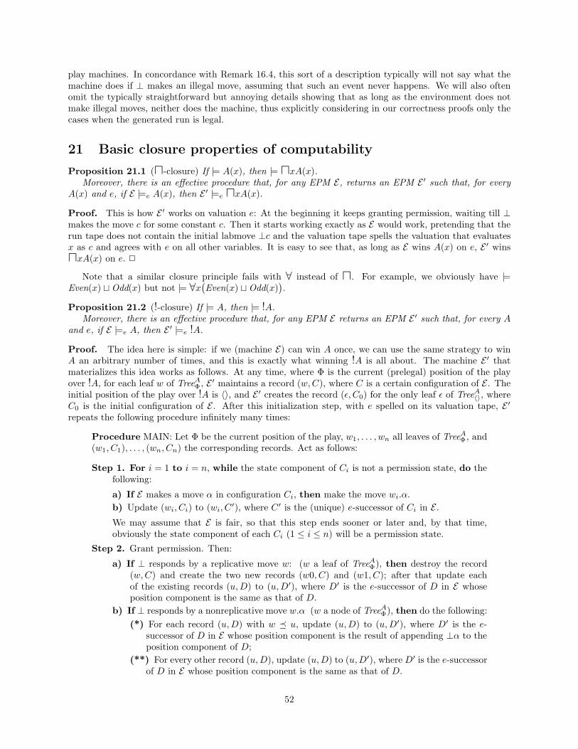
play machines. In concordance with Remark 16.4, this sort of a description typically will not say what themachine does if ⊥ makes an illegal move, assuming that such an event never happens. We will also oftenomit the typically straightforward but annoying details showing that as long as the environment does notmake illegal moves, neither does the machine, thus explicitly considering in our correctness proofs only thecases when the generated run is legal.

21 Basic closure properties of computability

Proposition 21.1 (u-closure) If |= A(x), then |= uxA(x).Moreover, there is an effective procedure that, for any EPM E, returns an EPM E ′ such that, for every

A(x) and e, if E |=e A(x), then E ′ |=e uxA(x).

Proof. This is how E ′ works on valuation e: At the beginning it keeps granting permission, waiting till ⊥makes the move c for some constant c. Then it starts working exactly as E would work, pretending that therun tape does not contain the initial labmove ⊥c and the valuation tape spells the valuation that evaluatesx as c and agrees with e on all other variables. It is easy to see that, as long as E wins A(x) on e, E ′ winsuxA(x) on e. 2

Note that a similar closure principle fails with ∀ instead of u. For example, we obviously have |=Even(x) t Odd(x) but not |= ∀x

(Even(x) t Odd(x)

).

Proposition 21.2 (!-closure) If |= A, then |= !A.Moreover, there is an effective procedure that, for any EPM E returns an EPM E ′ such that, for every A

and e, if E |=e A, then E ′ |=e !A.

Proof. The idea here is simple: if we (machine E) can win A once, we can use the same strategy to winA an arbitrary number of times, and this is exactly what winning !A is all about. The machine E ′ thatmaterializes this idea works as follows. At any time, where Φ is the current (prelegal) position of the playover !A, for each leaf w of TreeA

Φ , E ′ maintains a record (w, C), where C is a certain configuration of E . Theinitial position of the play over !A is 〈〉, and E ′ creates the record (ε, C0) for the only leaf ε of TreeA

〈〉, whereC0 is the initial configuration of E . After this initialization step, with e spelled on its valuation tape, E ′

repeats the following procedure infinitely many times:

Procedure MAIN: Let Φ be the current position of the play, w1, . . . , wn all leaves of TreeAΦ , and

(w1, C1), . . . , (wn, Cn) the corresponding records. Act as follows:

Step 1. For i = 1 to i = n, while the state component of Ci is not a permission state, do thefollowing:

a) If E makes a move α in configuration Ci, then make the move wi.α.b) Update (wi, Ci) to (wi, C

′), where C ′ is the (unique) e-successor of Ci in E .

We may assume that E is fair, so that this step ends sooner or later and, by that time,obviously the state component of each Ci (1 ≤ i ≤ n) will be a permission state.

Step 2. Grant permission. Then:

a) If ⊥ responds by a replicative move w: (w a leaf of TreeAΦ), then destroy the record

(w, C) and create the two new records (w0, C) and (w1, C); after that update eachof the existing records (u, D) to (u, D′), where D′ is the e-successor of D in E whoseposition component is the same as that of D.

b) If ⊥ responds by a nonreplicative move w.α (w a node of TreeAΦ), then do the following:

(*) For each record (u, D) with w � u, update (u, D) to (u, D′), where D′ is the e-successor of D in E whose position component is the result of appending ⊥α to theposition component of D;

(**) For every other record (u, D), update (u, D) to (u, D′), where D′ is the e-successorof D in E whose position component is the same as that of D.

52

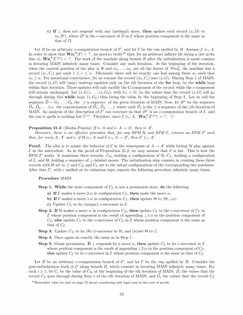
c) If ⊥ does not respond with any (prelegal) move, then update each record (u, D) to(u, D′), where D′ is the e-successor of D in E whose position component is the same asthat of D.

Let B be an arbitrary e-computation branch of E ′, and let Γ be the run spelled by B. Assume E |=e A.In order to show that Wn!A

e 〈Γ〉 = >, we need to verify10 that, for an arbitrary infinite bit string u (let us fixthis u), WnA

e 〈Γ�u〉 = >. The work of the machine along branch B after the initialization is made consistsin iterating MAIN infinitely many times. Consider any such iteration. At the beginning of the iteration,when the current position of the play is Φ and w1, . . . , wn are all the leaves of TreeA

Φ , the machine has arecord (wi, Ci) per each 1 ≤ i ≤ n. Obviously there will be exactly one leaf among these wi such thatwi � u. For notational convenience, let us rename the record (wi, Ci) into (s, G). During Step 1 of MAIN,the record (s, G) will (may) undergo updates only on the ith iteration of the for loop, by the while loopwithin that iteration. These updates will only modify the G component of the record, while the s componentwill remain unchanged. Let (s, G1), . . . , (s, Gk), with G1 = G, be the values that the record (s, G) will gothrough during this while loop, (s, Gk) thus being the value by the beginning of Step 2. Let us call thesequence ~D = G1, . . . , Gk the � u-sequence of the given iteration of MAIN. Now, let Bu be the sequence~D1, ~D2, . . . (i.e. the concatenation of ~D1, ~D2, . . . ), where each ~Dj is the � u-sequence of the jth iteration ofMAIN. An analysis of the description of E ′ can convince us that Bu is an e-computation branch of E , andthe run it spells is nothing but Γ�u. Therefore, since E |=e A, WnA

e 〈Γ�u〉 = >. 2

Proposition 21.3 (Modus Ponens) If |= A and |= A → A′, then |= A′.Moreover, there is an effective procedure that, for any HPM H and EPM E, returns an EPM E ′ such

that, for every A, A′ and e, if H |=e A and E |=e A → A′, then E ′ |=e A′.

Proof. The idea is to mimic the behavior of E in the consequent of A → A′ while letting H play againstE in the antecedent. As in the proof of Proposition 21.2, we may assume that E is fair. This is how theEPM E ′ works. It maintains three records: CH, holding a configuration of H, CE , holding a configurationof E , and Θ, holding a sequence of ⊥-labeled moves. The initialization step consists in creating these threerecords with Θ set to 〈〉 and CH and CE set to the initial configurations of the corresponding two machines.After that E ′, with e spelled on its valuation tape, repeats the following procedure infinitely many times:

Procedure MAIN:

Step 1. While the state component of CE is not a permission state, do the following:

a) If E makes a move 2.α in configuration CE , then make the move α.b) If E makes a move 1.α in configuration CE , then update Θ to 〈Θ,⊥α〉.c) Update CE to its (unique) e-successor in E .

Step 2. If H makes a move α in configuration CH, then update CE to the e-successor of CE inE whose position component is the result of appending ⊥1.α to the position component ofCE ; else update CE to the e-successor of CE in E whose position component is the same asthat of CE .

Step 3. Update CH to its (Θ, e)-successor in H, and (re)set Θ to 〈〉.Step 4. Once again do exactly the same as in Step 1.

Step 5. Grant permission. If ⊥ responds by a move α, then update CE to its e-successor in Ewhose position component is the result of appending ⊥2.α to the position component of CE ;else update CE to its e-successor in E whose position component is the same as that of CE .

Let B be an arbitrary e-computation branch of E ′, and let Γ be the run spelled by B. Consider thepost-initialization work of E ′ along branch B, which consists in iterating MAIN infinitely many times. Foreach i ≥ 1, let Ci be the value of CH at the beginning of the ith iteration of MAIN, ~Di the values that therecord CE goes through during Step 1 of the ith iteration of MAIN, and ~Gi the values that the record CE

10Remember what we said on page 52 about considering only legal runs in this sort of proofs.

53

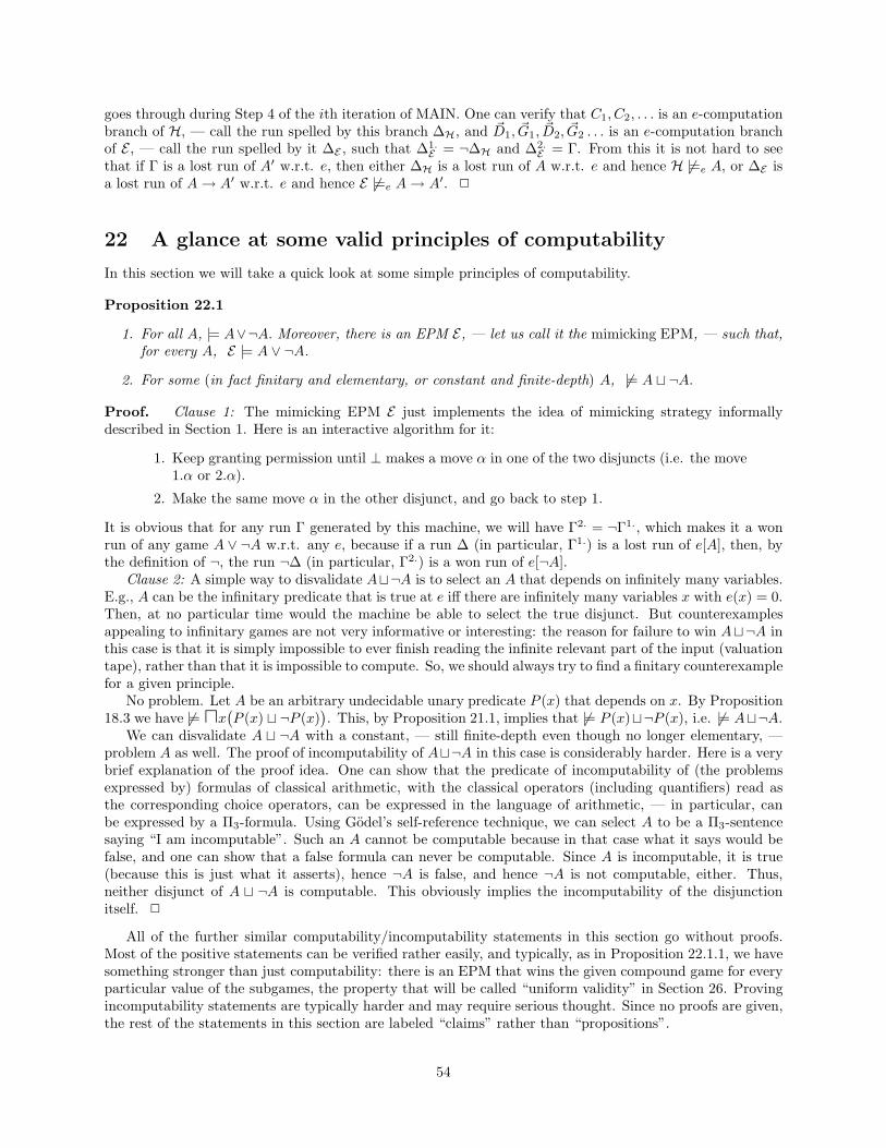
goes through during Step 4 of the ith iteration of MAIN. One can verify that C1, C2, . . . is an e-computationbranch of H, — call the run spelled by this branch ∆H, and ~D1, ~G1, ~D2, ~G2 . . . is an e-computation branchof E , — call the run spelled by it ∆E , such that ∆1.

E = ¬∆H and ∆2.E = Γ. From this it is not hard to see

that if Γ is a lost run of A′ w.r.t. e, then either ∆H is a lost run of A w.r.t. e and hence H 6|=e A, or ∆E isa lost run of A → A′ w.r.t. e and hence E 6|=e A → A′. 2

22 A glance at some valid principles of computability

In this section we will take a quick look at some simple principles of computability.

Proposition 22.1

1. For all A, |= A∨¬A. Moreover, there is an EPM E, — let us call it the mimicking EPM, — such that,for every A, E |= A ∨ ¬A.

2. For some (in fact finitary and elementary, or constant and finite-depth) A, 6|= A t ¬A.

Proof. Clause 1: The mimicking EPM E just implements the idea of mimicking strategy informallydescribed in Section 1. Here is an interactive algorithm for it:

1. Keep granting permission until ⊥ makes a move α in one of the two disjuncts (i.e. the move1.α or 2.α).

2. Make the same move α in the other disjunct, and go back to step 1.

It is obvious that for any run Γ generated by this machine, we will have Γ2. = ¬Γ1., which makes it a wonrun of any game A ∨ ¬A w.r.t. any e, because if a run ∆ (in particular, Γ1.) is a lost run of e[A], then, bythe definition of ¬, the run ¬∆ (in particular, Γ2.) is a won run of e[¬A].

Clause 2: A simple way to disvalidate At¬A is to select an A that depends on infinitely many variables.E.g., A can be the infinitary predicate that is true at e iff there are infinitely many variables x with e(x) = 0.Then, at no particular time would the machine be able to select the true disjunct. But counterexamplesappealing to infinitary games are not very informative or interesting: the reason for failure to win At¬A inthis case is that it is simply impossible to ever finish reading the infinite relevant part of the input (valuationtape), rather than that it is impossible to compute. So, we should always try to find a finitary counterexamplefor a given principle.

No problem. Let A be an arbitrary undecidable unary predicate P (x) that depends on x. By Proposition18.3 we have 6|= ux

(P (x) t ¬P (x)

). This, by Proposition 21.1, implies that 6|= P (x)t¬P (x), i.e. 6|= At¬A.

We can disvalidate A t ¬A with a constant, — still finite-depth even though no longer elementary, —problem A as well. The proof of incomputability of At¬A in this case is considerably harder. Here is a verybrief explanation of the proof idea. One can show that the predicate of incomputability of (the problemsexpressed by) formulas of classical arithmetic, with the classical operators (including quantifiers) read asthe corresponding choice operators, can be expressed in the language of arithmetic, — in particular, canbe expressed by a Π3-formula. Using Godel’s self-reference technique, we can select A to be a Π3-sentencesaying “I am incomputable”. Such an A cannot be computable because in that case what it says would befalse, and one can show that a false formula can never be computable. Since A is incomputable, it is true(because this is just what it asserts), hence ¬A is false, and hence ¬A is not computable, either. Thus,neither disjunct of A t ¬A is computable. This obviously implies the incomputability of the disjunctionitself. 2

All of the further similar computability/incomputability statements in this section go without proofs.Most of the positive statements can be verified rather easily, and typically, as in Proposition 22.1.1, we havesomething stronger than just computability: there is an EPM that wins the given compound game for everyparticular value of the subgames, the property that will be called “uniform validity” in Section 26. Provingincomputability statements are typically harder and may require serious thought. Since no proofs are given,the rest of the statements in this section are labeled “claims” rather than “propositions”.

54

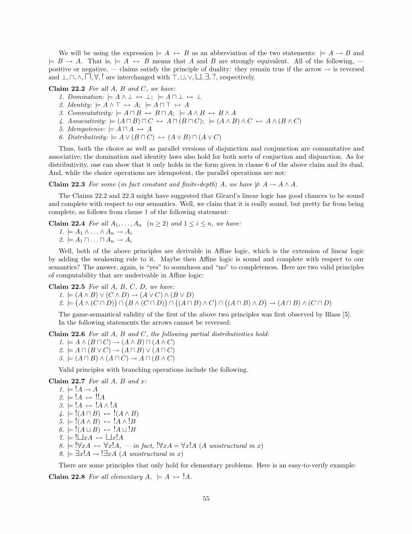
We will be using the expression |= A ↔ B as an abbreviation of the two statements: |= A → B and|= B → A. That is, |= A ↔ B means that A and B are strongly equivalent. All of the following, —positive or negative, — claims satisfy the principle of duality: they remain true if the arrow → is reversedand ⊥,u,∧,u,∀, ! are interchanged with >,t,∨,t,∃, ?, respectively.

Claim 22.2 For all A, B and C, we have:1. Domination: |= A ∧ ⊥ ↔ ⊥; |= A u ⊥ ↔ ⊥2. Identity: |= A ∧ > ↔ A; |= A u > ↔ A3. Commutativity: |= A u B ↔ B u A; |= A ∧ B ↔ B ∧ A4. Associativity: |= (A u B) u C ↔ A u (B u C); |= (A ∧ B) ∧ C ↔ A ∧ (B ∧ C)5. Idempotence: |= A u A ↔ A6. Distributivity: |= A ∨ (B u C) ↔ (A ∨ B) u (A ∨ C)

Thus, both the choice as well as parallel versions of disjunction and conjunction are commutative andassociative; the domination and identity laws also hold for both sorts of conjuction and disjunction. As fordistributivity, one can show that it only holds in the form given in clause 6 of the above claim and its dual.And, while the choice operations are idempotent, the parallel operations are not:

Claim 22.3 For some (in fact constant and finite-depth) A, we have 6|= A → A ∧ A.

The Claims 22.2 and 22.3 might have suggested that Girard’s linear logic has good chances to be soundand complete with respect to our semantics. Well, we claim that it is really sound, but pretty far from beingcomplete, as follows from clause 1 of the following statement:

Claim 22.4 For all A1, . . . , An (n ≥ 2) and 1 ≤ i ≤ n, we have:1. |= A1 ∧ . . . ∧ An → Ai

2. |= A1 u . . . u An → Ai

Well, both of the above principles are derivable in Affine logic, which is the extension of linear logicby adding the weakening rule to it. Maybe then Affine logic is sound and complete with respect to oursemantics? The answer, again, is “yes” to soundness and “no” to completeness. Here are two valid principlesof computability that are underivable in Affine logic:

Claim 22.5 For all A, B, C, D, we have:1. |= (A ∧ B) ∨ (C ∧ D) → (A ∨ C) ∧ (B ∨ D)2. |=

(A ∧ (C u D)

)u

(B ∧ (C u D)

)u

((A u B) ∧ C

)u

((A u B) ∧ D

)→ (A u B) ∧ (C u D)

The game-semantical validity of the first of the above two principles was first observed by Blass [5].In the following statements the arrows cannot be reversed:

Claim 22.6 For all A, B and C, the following partial distributivities hold:1. |= A ∧ (B u C) → (A ∧ B) u (A ∧ C)2. |= A u (B ∨ C) → (A u B) ∨ (A u C)3. |= (A u B) ∧ (A u C) → A u (B ∧ C)

Valid principles with branching operations include the following.

Claim 22.7 For all A, B and x:1. |= !A → A2. |= !A ↔ !!A3. |= !A ↔ !A ∧ !A4. |= !(A u B) ↔ !(A ∧ B)5. |= !(A ∧ B) ↔ !A ∧ !B6. |= !(A t B) ↔ !A t !B7. |= !txA ↔ tx!A8. |= !∀xA ↔ ∀x!A, — in fact, !∀xA = ∀x!A (A unistructural in x)9. |= ∃x!A → !∃xA (A unistructural in x)

There are some principles that only hold for elementary problems. Here is an easy-to-verify example:

Claim 22.8 For all elementary A, |= A ↔ !A.

55

23 Universal problems

When talking about computational problems, we often only consider elements of some fixed set of problems.In typical or at least most interesting cases such a set will be countable, and usually come with some standardenumeration of its elements, such as the lexicographic order of expressions representing the problems of theset. We call such enumerated sets “problem universes”:

Definition 23.1 A problem universe is a sequence of problems.

Such a sequence can be finite or infinite. However, for convenience and without loss of generality, wewill assume that all problem universes that we consider are infinite, for a finite problem universe can alwaysbe rewritten as an “equivalent” infinite universe by replicating its last problem infinitely many times. Also,even though, strictly speaking, a problem universe should be a sequence rather than a set, we will oftendescribe a universe just by explaining what problems are in it, i.e. present it as a set of problems ratherthan a sequence of problems. This can be done when how those elements are arranged in the sequence isirrelevant, or when there is some obvious, standard arrangement such as the one based on the lexicographicorder of the (possibly multiple) names of the problems of the universe. In any case, when we write A ∈ Ufor a given problem universe U , we mean that problem A appears (possibly with repetitions) in U .

For problems A and B, let us call any EPM that wins A → B an EPM-reduction of B to A.

Definition 23.2 Let U = 〈A1, A2, . . .〉 be a problem universe. A universal problem of U is a problem $ suchthat:

1. Each Ai ∈ U is reducible to $ and,

2. furthermore, there is an effective procedure that, for each i ≥ 1, returns an EPM-reduction of Ai to $.

The intuition behind the concept of universal problem $ is that this is a problem of universal strength:having it as a computational resource means being able to solve any of the problems of the universe asevery problem of the universe is algorithmically reducible to $. However, just existence of those algorithmicreductions would have little value if there was no way to find them. The ‘furthermore’ clause of the abovedefinition guarantees that reduction strategies not only exist, but can be effectively found.

It is evident that ⊥ is a universal problem of every problem universe U . Furthermore, if U contains aproblem whose negation is computable, then every universal problem of U will be equivalent to ⊥. However,the concept of universal problem is more general than ⊥. E.g., some natural problem universes may entirelyconsist of positive problems, in which case a much weaker, — in particular, positive, — problem can serve asa universal problem. The acceptance problem for the universal Turing machine, which of course is positive,would obviously be a universal problem for the universe that consists of acceptance problems for all particularTuring machines (with those problems arranged, say, in the lexicographic order of their standard descriptions,or standard descriptions of the corresponding Turing machines).

A universal problem does not necessarily have to be 0-ary. Here is a natural example. Let x range oversome set T of axiomatic theories (all in the same language) based on first-order classical logic, with notnecessarily recursive or consistent sets of axioms; let y range over formulas of the language of those theories,and z range over finite sequences of such formulas; let Proof(x, y, z) be the predicate “z is a proof of y inx”. Then $ = tzProof(x,⊥, z), i.e. the problem of finding a proof of the absurd in theory x, will be auniversal problem for the universe U = {tzProof(x, F, z) | F is a formula}, which consists of the problemsof finding proofs in a given theory x for various particular formulas. Notice that if all theories from T areinconsistent, then the entire universe U (that includes $) exclusively consists of positive problems; at thesame time, unless T is finite or all theories from T are recursively enumerable, $ and some other problemsfrom U could be incomputable.

The list of strict mathematical examples of problem universe / universal problem pairs illustrating themeaning and usefulness of the idea of universal problem could be continued of course. But this idea isso natural that it can as well be explained in nonmathematical terms to laymen or even little children:understanding problems in a very general — not-only-computational — sense (see Section 26), the problemof catching the gold fish is a universal problem of the universe {Making W come true | W is any wish}.

56

In view of the resource intuition associated with our semantics (again, see Section 26 for a detaileddiscussion), our selection of symbol $ for universal problems is no accident: money, — an adult’s gold fish,— is a good example of a universal resource, a resource that can be converted into any other resource in theworld where everything can be bought.

According to condition 2 of Definition 23.2, there is an effective procedure that finds a reduction of anygiven element of the problem universe to the universal problem. Generally, however, this procedure could bedifferent for different problem universe / universal problem pairs, which would eventually make it impossibleto treat $ as a logical or semi-logical symbol as we are going to do in the next section. Fortunately thereis a way to standardize the reduction procedure so that it will be common for universal problems of alluniverses, that is, an element A of a problem universe can be reduced to a universal problem $ of thatuniverse without knowing what particular problems A and $ really are. This effect is achieved by restrictinguniversal problems to what we call “standard universal problems” (Definition 23.3). Such a restriction doesnot yield loss of generality because every universal problem turns out to be equivalent to and hence canbe thought of as some standard universal problem (Proposition 23.4). Putting it another way, standarduniversal problems can be considered standard representatives of equivalence classes of universal problemsand in most contexts can be identified with them.

Definition 23.3 Let U = 〈A1, A2, A3, . . .〉 be a problem universe.

1. For a problem A0, the A0-based standard universal problem of U is the problem $ defined as follows:

• Lr$e = {〈〉} ∪ {〈⊥i, Γ〉 | i ∈ {0, 1, 2, . . .}, Γ ∈ LrAi

e }.

• Wn$e〈〉 = >; Wn$

e〈⊥i, Γ〉 = WnAie 〈Γ〉.

2. A standard universal problem $ of U is the A0-based standard universal problem of U for some problemA0; the latter is said to be the base of $.

Notice that the A0-based standard universal problem $ of U = 〈A1, A2, . . .〉 is nothing but what can becalled the infinite additive conjunction A0 uA1 uA2 u . . .. Obviously we could show that the infinite versionof additive conjunction preserves the static property of games in the same way as we did for finite additiveconjunctions in Section 10, so $ indeed is a problem (static game). It is also easy to see that $ is indeed auniversal problem of U . The strategy that wins $ → Ai for the ith element of U is to select the conjunctAi of the infinite conjunction $ thus bringing the game down to Ai → Ai, and then continue the rest of theplay as the mimicking EPM described in the proof of Proposition 22.1.1. Notice that, as we claimed a whileago, this strategy is indeed “uniform” in that it does not require any specific knowledge of $ or Ai.

Proposition 23.4 Suppose U is a problem universe and A0 a universal problem of U . Then A0 is equivalentto the A0-based standard universal problem of U .

Proof. Let U = 〈A1, A2, . . .〉 be a problem universe, A0 a universal problem of U , and $ the A0-basedstandard universal problem of U . We need to show that |= $ → A0 and |= A0 → $. The former is obvious:$ → A0 will be won by an EPM that makes the move 1.0 and continues playing the resulting game A0 → A0

using the mimicking strategy.Let now f be an effective function that, for each i ≥ 1, returns (the description of) an EPM that wins

A0 → Ai. Such a function exists according to clause 2 of Definition 23.2. We extend the domain of f to 0by letting f(0) be the mimicking EPM that wins A0 → A0. Here is a very relaxed description of an EPM Ethat wins A0 → $ on an arbitrary valuation e. As always (Remark 16.4), this description assumes that theenvironment never makes illegal moves. The work of E consists of three stages.

During stage 1, E keeps granting permission until ⊥ selects a conjunct Ai in the consequent, rememberingthe moves α1, . . . , αn that ⊥ may meanwhile make in the antecedent. We may assume that such a selectionof Ai will be made sooner or later, for otherwise E clearly wins.

During stage 2, using f , E finds an EPM Ei that wins A0 → Ai. In view of Theorem 17.2, we mayassume that Ei is fair. Then E traces/simulates, on its work tape, the work of Ei up to the configuration Cwhen Ei grants its (n + 1)th permission, remembering the moves β1, . . . , βm that Ei makes meanwhile. This

57

simulation assumes that to each jth permission (1 ≤ j ≤ n) the environment responded by the move 1.αj ,and that the valuation tape of Ei spells the same e as the valuation tape of E .

At the beginning of stage 3, E makes the above moves β1, . . . , βm. After that it plays the rest of the gameas Ei (with e on its valuation tape) would play starting from configuration C. That is, E resumes simulationof Ei only, unlike stage 2, now every time it sees that Ei made a move, E also makes the same move, andevery time it sees that Ei granted permission, E also grants permission and then copies ⊥’s response to thesimulated run tape contents of Ei.

The run generated by E in the above scenario will thus look like 〈⊥1.α1, . . . ,⊥1.αn,⊥2.i,>β1, . . . ,>βm, ∆〉.One can see that this is a won run of e[A0 → $] if Γ = 〈⊥1.α1, . . . ,⊥1.αn,>β1, . . . ,>βm, ∆〉 is a won run ofe[A0 → Ai]. Let Γi be the run spelled by the computation branch of Ei that was simulated by E . ObviouslyΓi = 〈Θ, ∆〉 for some Θ such that 〈⊥1.α1, . . . ,⊥1.αn,>β1, . . . ,>βm〉 is a >-delay of Θ. Hence Γ is a >-delayof Γi and, as the latter is a won run of e[A0 → Ai] (because Ei |= A0 → Ai), so is the former. 2

24 The universal language

The author could continue in the style of Section 22 and try to come up with a complete list of all validprinciples of computability. But the publisher insists that the lengths of submitted papers be finite, so analternative way has to be found. This section introduces a formal language, called the universal language,in which we may want to try to axiomatize the set of valid principles.

This is a comprehensive first-order specification language for computational problems with the same setVariables of variables as the one we fixed in Part I. A distinguishing feature of this language is that ithas two sorts of problem letters (called “predicate letters” in classical logic): elementary letters and generalletters. With each (elementary or general) letter is associated an integer n ≥ 0 called its arity. Letters aredivided into two categories: nonlogical and logical. For each n, there are infinitely many n-ary elementaryand general nonlogical letters. As for logical letters, there are three of them, all 0-ary: two elementary logicalletters ⊥ and >, and one general logical letter $. Where L is a (logical or nonlogical, elementary or general)n-ary letter and x1, . . . , xn any variables, the expression L(x1, . . . , xn) is called a (logical or nonlogical,elementary or general) n-ary atom. Thus, each 0-ary letter is, at the same time, an atom. Formulas are builtfrom atoms in the standard way using the operators ¬, ∧, ∨, →, u, t, !, ?, ⇒, ∀, ∃, u, t. Henceforth by“formula” we always mean a formula of the universal language unless otherwise specified.

The definition of the scope of a given occurrence of a logical operator is standard. For quantifiers wealso need a more restricted concept of scope called immediate scope. Let F be a formula, O a particularoccurrence of a certain subexpression in F , x a variable, and Q one of the quantifiers ∀,∃,u,t. We saythat O is in the immediate scope of Qx in F iff F has a subformula QxG such that O is in G and, if G hasa subformula Q′xG′ where Q′ is a quantifier, then O is not in G′. Example: where x and y are distinctvariables, the first occurrence of P (x, y) in ∀x∃y(P (x, y)uQ →uxP (x, y)) is in the immediate scope of ∀xas well as ∃y; the second occurrence is in the immediate scope of ux as well as ∃y; it is in the scope but notin the immediate scope of ∀x because ∀x is “overridden” by ux. The definition of what a free occurrence ofvariable x means is also standard: such an occurrence is free iff it is not in the scope of ∀x,∃x,ux or tx;otherwise it is bound.

In the spirit of Convention 7.3 we will sometimes fix a certain tuple x1, . . . , xn of distinct variables for agiven formula F and write F as F (x1, . . . , xn). Then the expression F (y1, . . . , yn) will stand for the resultof replacing all free occurrences of x1, . . . , xn in F (x1, . . . , xn) by y1, . . . , yn, respectively. It should be notedthat when representing F as F (x1, . . . , xn), we usually do not mean that x1, . . . , xn are all the free variablesof F , nor do we mean that each of these variables has a free occurrence in F .

Definition 24.1 An interpretation is a function ∗ that assigns, to every elementary (resp. general) n-aryletter L, an elementary (resp. static) game ∗L with an attached tuple of n (distinct) variables such that thefollowing conditions are satisfied:

1. ∗⊥ = ⊥ and ∗> = >.

58

2. ∗$ is a standard universal problem of the universe

{C | C is a tuple-instantiation of ∗L for some general nonlogical letter L}.

Where L is an n-ary letter with ∗L = A(x1, . . . , xn) and c1, . . . , cn are constants, the expression“L(c1, . . . , cn)” is considered a name of the problem A(c1, . . . , cn), and the elements of the aboveuniverse are assumed to be arranged in a sequence according to the lexicographic order of their names.

When B is the base of ∗$ (as a standard universal problem), interpretation ∗ is said to be B-based.

Definition 24.2 For a formula F , an F -admissible interpretation is an interpretation ∗ such that, for eachn-ary letter L with ∗L = A(x1, . . . , xn), the following two conditions are satisfied:

1. A(x1, . . . , xn) does not depend on any of the variables that are not among x1, . . . , xn but occur in F .

2. If, for some y1, . . . , yn and 1 ≤ i ≤ n, F has an occurrence of the atom L(y1, . . . , yn) that is in theimmediate scope of ∀yi or ∃yi, then A(x1, . . . , xn) is unistructural in xi.

We turn such an interpretation ∗ into a function that assigns a problem G∗ to each subformula G of F asfollows:

• Where L is an n-ary letter with ∗L = A(x1, . . . , xn) and y1, . . . , yn are any variables,(L(y1, . . . , yn)

)∗ =A(y1, . . . , yn);

• (¬G)∗ = ¬(G∗); similarly for !, ?;• (G → H)∗ = G∗ → H∗; similarly for ⇒;• (G1 ∧ . . . ∧ Gn)∗ = G∗

1 ∧ . . . ∧ G∗n; similarly for ∨,u,t;

• (uxG)∗ = ux(G∗); similarly for t,∀,∃.

When saying “an interpretation of F”, we mean the problem F ∗ for some F -admissible interpretation∗. When ∗ is an F -admissible interpretation with F ∗ = A, we say that ∗ interprets F as A. The sameterminology applies to letters: we will say that interpretation ∗ interprets letter L as the problem ∗L.

Thus, (admissible) interpretations turn formulas of the universal language into particular problems,interpreting elementary atoms as elementary problems, general atoms as any problems, and logical operatorsas the same-name game operations. The main reason for having two sorts of atoms in the language is to makeit more expressive: the point is that whether a given principle of computability is valid may greatly dependon whether the problems it involves are elementary or not; since our language can capture the differencebetween elementary and general (not necessarily elementary) problems, it allows us to describe computabilityprinciples at a finer level. Another reason for having elementary atoms along with general atoms is that, aswe are going to see in the next section, this can make the job of axiomatizing the logic easier.

Each interpretation induces a natural problem universe, — the one consisting of all tuple-instantiationsof the interpretations of general letters. According to the above definition, $ is interpreted as a universalproblem of that universe. Adding to the language an “elementary counterpart” of $, — i.e. an elementarylogical letter that would be interpreted as a universal problem of the universe that consists of all tuple-instantiations of the interpretations of elementary letters, — would not make much sense. Indeed, ⊥ is anelementary letter and hence the game ⊥ (= ∗⊥) is in the above universe. Therefore, as we noted in theprevious section, any universal problem of such a universe would be equivalent to ⊥ and hence equal to ⊥because for elementary games equivalence means equality. Thus, ⊥ in fact acts as what can be consideredan elementary counterpart of $. Generally, the concept of universal problem is interesting and nontrivialonly in the context of nonelementary games.

Notice that our definition of interpretation does not insist that an n-ary letter be interpreted as ann-ary game. There are no strong reasons for imposing this requirement. On the other hand, with such arequirement generality would be lost, for we would no longer be able to capture infinitary problems. Somegenerality would be lost even if we agreed to restrict our considerations to finitary games only. For example,in order to show that all finitary problems of the form A ∨ ¬A are computable, we would have to prove thevalidity of each of the infinitely many formulas: P ∨¬P , Q(x)∨¬Q(x), R(x, y)∨¬R(x, y), . . . ., corresponding

59

to the infinitely many different possible finite arities for A. But in our approach, which allows the 0-arygeneral letter P to be interpreted as any (constant or non-constant, finitary or infinitary, elementary ornon-elementary) problem, just showing the validity of P ∨¬P would be sufficient to automatically concludethat all games of the corresponding form are computable no matter what their arities are.

Thus, the game ∗L = A(x1, . . . , xn) for an n-ary letter L may depend on some hidden variables beyondits explicit variables x1, . . . , xn. According to condition 1 of Definition 24.2, however, those hidden variablesshould remain hidden all the time and never explicitly occur in formulas. This sort of a restriction is necessaryto prevent certain unpleasant collisions of variables. For example, if L is a unary letter interpreted as A(x)where A(x) is the predicate x > y, y would be a hidden variable. If y was allowed to appear in subformulasof a given formula, then, even though the two (sub)formulas L(x) and L(y) would “look similar”, they wouldrepresent rather different predicates: L(x) represent x > y while L(y) represent y > y which is nothingbut ⊥, so that certain classically valid principles such as ∃xL(x) → ∃yL(y) would fail. Another exampleof a pair of formulas that look similar but whose interpretations would be far from being similar is ∀zA(x)and ∀yA(x). All unsettling examples of this sort, however, would involve formulas that contain the hiddenvariable y. Condition 1 amounts to excluding such formulas from the language.

And the purpose of condition 2 of Definition 24.2 is to guarantee that F ∗ is always defined. The point isthat, unlike any other logical operators, the game operations represented by ∀x and ∃x may be undefined forsome arguments, — in particular, arguments that are not x-unistructural. It can be verified by induction oncomplexity that, as long as both conditions of Definition 24.2 are satisfied and ∀xG or ∃xG is a subformulaof F , the game G∗ is (defined and) x-unistructural, so that ∀xG∗ and ∃xG∗ are defined.

Definition 24.3 A formula of the universal language is said to be valid iff every interpretation of it iswinnable.

Thus, valid formulas represent valid principles of computability, — they can be thought of as schemataof “always computable” problems. Every nontrivial completeness result, — result establishing that noneof the formulas from (or beyond) a given class is valid, — will carry negative information in that it willestablish some limitations of computability. The strength of such negative information, however, wouldgenerally greatly depend on what kind of interpretations are used in counterexamples when proving non-validity. First and foremost, we do not want those counterexamples to appeal to infinitary or indeterminedproblems. As this was pointed out in the proof of Proposition 22.1.2, a (positive) infinitary game may failto be winnable just because it is impossible to ever finish reading all the relevant input information fromthe valuation tape, which would generally make powerless not only algorithmic strategies but any strategiesas well that do not have full actual knowledge of the infinite contents of the valuation tape. Similarly, allindetermined problems are incomputable because they simply have no solutions (even by God), so thatindetermined counterexamples will never illustrate any limitations specific to algorithmic methods. Thefollowing conjecture immensely strengthens all possible nontrivial completeness results:

Conjecture 24.4 If a formula F of the universal language is not valid, then F ∗ is not winnable for someF -admissible interpretation ∗ that interprets all atoms as finitary, determined, strict, unistructural problems.

Conjecture 25.4 (clause 2) of the following section strengthens the above statement for the exponential-free fragment of the universal language by further restricting the range of ∗ to finite-depth problems. Sodoes Conjecture 25.8 for another natural and rich fragment of the language. It would be interesting to knowif such a restriction extends to the full universal language as well. Most likely it does. Very good if so:the more restricted the range of interpretations is, the more general, informative, interesting and strong thecorresponding completeness/non-validity results are.

25 The universal logic

Definition 25.1 The universal logic is the set of all valid formulas of the universal language.

Here is the naturally arising main open problem in computability logic: Is the universal logic recursivelyenumerable and, if yes, does it have a reasonable axiomatization?

60

In view of the extraordinary expressive strength of the universal language, solving this big open problemin full generality, — if the answer is positive, — is a presumably challenging task. A reasonable way togo would be not to try to attack the problem at once, but approach it step-by-step by exploring, in anincremental way, fragments of the universal logic obtained by imposing some natural restrictions on itslanguage.

One of the natural fragments of the universal logic is obtained by forbidding in its language general letters(including $) and the operators that do not preserve the elementary property of games, which, in view ofTheorem 14.1, only leaves the operators ¬,∧,∨,→,∀,∃, so that we get exactly the language of classicalpredicate calculus CL. This fragment can be called the logic of elementary problems as all of its formulas(and only those formulas) represent elementary problems. A simple analysis of our definitions of the abovegame operations reveals that, when applied to elementary games (predicates), their semantical meaning isexactly classical, i.e. solvability of an interpretation F ∗ of a formula F of the above fragment means nothingbut its classical truth. Of course, the traditional concept of classical validity and the corresponding soundnessproofs for CL deal only with the case of finitary predicates and require that every n-ary letter be interpretedas an n-ary predicate. The more general and relaxed approach that we have taken, however, hardly createsany difference: condition 1 of Definition 24.2 guarantees that all of the possible hidden variables on which theinterpretation of a given atom may depend will remain totally neutral and harmless, so that CL continuesto be sound. This fact, together with Godel’s completeness theorem for CL, yields the following proposition,establishing that the universal logic is a conservative extension of CL so that the latter is a natural syntacticfragment of the former:

Proposition 25.2 CL ` F iff F is valid (any formula F of the language of CL).Moreover, if CL 6` F , then F ∗ is not winnable for some F -admissible interpretation ∗ that interprets all

atoms as finitary predicates.

Another natural fragment of the universal logic, that we can call the logic of finite-depth problems, isobtained by forbidding in the universal language the only non-finite-depth operators !, ?,⇒. Let us callthis language the finite-depth language and its formulas finite-depth formulas. Obviously the logic of finite-depth problems is not decidable as it contains classical predicate logic. However, according to Conjecture25.4 stated below, this logic is recursively enumerable and reasonably axiomatizable. This is a very strongpositive statement taking into account that the finite-depth language, even though smaller than the universallanguage, is still by an order of magnitude more expressive than the language of classical logic, and in factit is more expressive than the simple union of the languages of classical and additive-multiplicative linearlogics.

To axiomatize the logic of finite-depth games, we need some preliminary definitions. In this paragraph“formula” always means “finite-depth formula”. Understanding A → B as an abbreviation for ¬A ∨ B, apositive (resp. negative) occurrence of a subformula is an occurrence that is in the scope of an even (resp.odd) number of occurrences of ¬. By an elementary formula here we mean a formula that does not containgeneral letters, u,t,u or t; a surface occurrence of a subformula is an occurrence that is not in the scopeof u,t,u or t; and the elementarization of a formula F is the result of replacing in F all positive (resp.negative) surface occurrences of general atoms, — including $, — by ⊥ (resp. >), all (positive or negative)surface occurrences of the form G1u . . .uGn or uxG by >, and all (positive or negative) surface occurrencesof the form G1 t . . . tGn or txG by ⊥. We say that a formula F is stable iff its elementarization is a validformula of classical logic. Otherwise F is instable.

Definition 25.3 FD is the system in the finite-depth language given by the following rules of inference:

A. ~H ` F , where F is stable and ~H is a (minimal, finite) set of formulas satisfying the following conditions:

(i) If F has a positive (resp. negative) surface occurrence of a subformula G1 u . . . u Gn (resp.G1 t . . .tGn), then, for each i ∈ {1, . . . , n}, ~H contains the result of replacing this occurrence inF by Gi;

(ii) If F has a positive (resp. negative) surface occurrence of a subformula uxG(x) (resp. txG(x)),then ~H contains the result of replacing this occurrence in F by G(y) for some y not occurring inF .

61

B1. F ′ ` F , where F ′ is the result of replacing in F a negative (resp. positive) surface occurrence of asubformula G1 u . . . u Gn (resp. G1 t . . . t Gn) by Gi for some i ∈ {1, . . . , n}.

B2. F ′ ` F , where F ′ is the result of replacing in F a negative (resp. positive) surface occurrence of asubformula uxG(x) (resp. txG(x)) by G(y); here y is an arbitrary variable such that neither theabove occurrence of uxG(x) (resp. txG(x)) in F nor any of the free occurrences of x in G(x) are inthe scope of ∀y, ∃y, uy or ty.

C. F ′ ` F , where F ′ is the result of replacing in F two, — one positive and one negative, — surfaceoccurrences of some n-ary general letter by an n-ary nonlogical elementary letter that does not occurin F .

D. F ′ ` F , where F ′ is the result of replacing in F a negative surface occurrence of $ by a general n-aryatom L(x1, . . . , xn) such that the above occurrence of $ in F is not in the scope of ∀xi or ∃xi (any1 ≤ i ≤ n).

Axioms are not explicitly stated, but note that the set ~H of premises of Rule A can be empty, in whichcase the conclusion of that rule acts as an axiom.

Conjecture 25.4 FD ` F iff F is valid (any finite-depth formula F ). Moreover:a) There is an effective procedure that takes an FD-proof of a formula F and constructs an EPM that

wins F ∗ for every F -admissible interpretation ∗.b) If FD 6` F , then F ∗ is not winnable for some F -admissible interpretation ∗ that interprets all atoms

as finite-depth, finitary, strict, unistructural problems.

As long as we only consider interpretations that interpret atoms as finite-depth problems, all problemsexpressible in the language of FD will be finite-depth, because all the operators allowed in it preserve thefinite-depth property of games. In view of clause (b) of the above conjecture, the completeness of FD (andof course its soundness as well) will still be retained in this case. This is what allows us to call FD “thelogic of finite-depth problems”. For the same reason, FD is also a logic of perifinite-depth problems. Apreliminary version of this logic was studied in [15, 16].

Obviously FD is recursively enumerable. One can also show that

Claim 25.5 The ∀,∃-free fragment of FD is decidable.

This is a nice and perhaps not very obvious/expected fact, taking into account that the above fragmentof FD is still a first order logic as it contains the quantifier-type operators u and t. This fragment isalso natural as it gets rid of the only operators of the universal language that produce games with imperfectinformation. For this reason, it can be called the logic of perfect-information finite-depth games. Since Claim25.5 is of interest only modulo Conjecture 25.4, we let its proof wait till Conjecture 25.4 is officially verified,and hence label it “claim” rather than “proposition”.

Below come two other claims, stated without proofs for similar reasons.An elementary-base (resp. general-base) formula of the universal language is a formula not containing

general (resp. elementary) letters. Correspondingly, we will call the restriction of a logic to elementary-base(resp. general-base) formulas the elementary-base (resp. general-base) fragment of that logic.

Claim 25.6 The elementary-base fragment of FD, that can be called the elementary-base logic of finite-depth games, is exactly11 the logic L introduced in [14].

In [14], L was shown to be sound and complete with respect to a semantics that was technically ratherdifferent from our present semantics.12 The underlying philosophy for that semantics was understandingformulas as physical tasks (rather than computational problems). See Section 26 for a discussion of the taskintuition behind game semantics.

11Ignoring the minor differences between the languages of L and the elementary-base fragment of FD.12The propositional version of L, called TSKp, was studied in [13].

62

Claim 25.7 The general-base, ∀,∃, $-free fragment of FD is exactly the logic ET introduced in [12].

ET is a decidable first order system defined in [12] syntactically but not axiomatically. It was proven to besound and complete with a (yet another) semantics in mind that also was technically quite different from ourpresent semantics, — first of all because, as noted in Section 3, it only dealt with strict games. ET, in turn,was shown to be a conservative extension of the (only) two syntactic fragments of the logic induced by Blass’s[5] semantics for which decidability or completeness proofs are known, — specifically, the multiplicativepropositional fragment and the additive fragment (sequents containing only additive operators). The fact thatdifferent semantics, defined in different technical terms with different underlying motivations/philosophiesand by different authors, still yield the same relevant fragments of the universal logic, is one of the strongindications that the logic is natural and something indeed “real” stands behind it. Conjecture 25.8 statedshortly reinforces this view.

Another interesting fragment of the universal language, that can be thought of as the language of Heyt-ing’s intuitionistic predicate calculus INT, is the general-base fragment of the language whose only logicaloperators are u,t,u,t,⇒ and $, corresponding to the intuitionistic conjunction, disjunction, universalquantifier, existential quantifier, implication and absurd, respectively. Let us call this fragment of theuniversal language the intuitionistic language. The following conjecture, if proven true, would signify aconvincing materialization of Kolmogorov’s (1932) well-known but rather abstract thesis according to whichintuitionistic logic is (or should be) a logic of problems.

Conjecture 25.8 INT` F iff F is valid (any formula F of the intuitionistic language). Moreover:a) There is an effective procedure that takes an INT-proof of a formula F and constructs an EPM that

wins F ∗ for every F -admissible interpretation ∗.b) If INT 6` F , then F ∗ is not winnable for some F -admissible interpretation ∗ that interprets all atoms

as finite-depth, finitary, strict, unistructural problems.

Godel in 1933 suggested a certain ‘provability’ interpretation for INT in a quite abstract sense. Thatabstract idea was refined and successfully materialized by Artemov [2] for the propositional fragment of INT.It would be interesting to understand connections between the computability and provability interpretationsof INT and, in particular, see if Artemov’s proof polynomials have good computability-logic counterpartsin terms of EPM-strategies and their combinations.

26 Applications in knowledgebase and resourcebase systems

The main motivation for introducing the formalism and semantics presented in this paper was computability-theoretic. The scope of the significance of this study, however, is not limited to computability theory. Inthis section we will make a digression from our central line and show how and why our logic is of interest inother, more applied areas of computer science, such as knowledgebase theory or the part of AI that studiesplanning and action.

The reason for the failure of the principle F t ¬F , as we saw in Section 22, was that the problemrepresented by this formula may have no algorithmic solution. The reason for the failure of this principle ina knowledgebase system can, however, be much simpler. Such a system may fail to win the game

Female(Sandy) t ¬Female(Sandy)

not because there is no algorithmic solution to it (of course there is one), but just because the system simplylacks sufficient knowledge that would allow it to determine the gender of Sandy. On the other hand, anysystem would be able to “solve” the problem

Female(Sandy) ∨ ¬Female(Sandy)

as this is an automatically won elementary game so that there is nothing to solve at all. Obviously theknowledge expressed by AtB is generally stronger than the knowledge expressed by A∨B. Yet the languageof classical logic fails to capture this difference and, — within the framework of the traditional approaches([20] etc.), — the modal “know that” operator 2, — with all the complications it entails (such as, say, the

63

messiness of the semantics and the non-semidecidability of the corresponding logic), — is needed to describethe stronger knowledge A t B, which would translate as 2A ∨ 2B. This simple example demonstrates themain point the author wants to convey here: our universal language can serve not only as a specificationlanguage for computational problems, but also as a convenient and comprehensive knowledge specificationlanguage, yet without any special knowledge operators in it!

In this context, formulas of our language represent (interactive, multistep, complex) queries. A formulawhose main operator is t or t can be understood as a question asked by the user, and a formula whosemain operator is u or u a question asked by the system.13 Consider the problem udtmCures(m, d),where Cures(m, d) means “medicine m cures disease d”. This formula is the following question asked by thesystem: “For what disease do you want me to find a cure?”. The user’s response can be “Pneumonia”. Thismove takes us to the position tmCures(m, Pneumonia). This is now a question asked by the user: “Whatmedicine cures pneumonia?”. The system’s response can be “Penicillin”, thus taking us to the final positionCures(Penicillin, Pneumonia). The system has been successful if penicillin is really a cure for pneumonia.

Multiplicative combinations of formulas may represent queries of a more complex structure, — parallelqueries where both of the participants may have simultaneous legal questions; !F is a query that can bere-used an arbitrary number of times, etc.

To get a better feel of multiplicatives as query operations, let us consider an example involving →. Aswe did not have enough chances to demonstrate the usage of the blind quantifier ∀, we will trow it intothe example as well. Let us make Cures a 3-ary predicate, with Cures(m, p, d) meaning “Medicine m willcure patient p of disease d”. And let Bloodtype(b, p) mean “b is the blood type of patient p”. Imagine aknowledgebase system that can determine, for each disease, a medicine that cures a patient of that disease,provided that the knowledgebase is told what that patient’s blood type is. A selection of the right medicinedepends only on the blood type and the disease, so that the system does not need to know who the patientreally is. This can be captured by quantifying the variable p with ∀ rather than u. The query that thesystem can solve can then be expressed by

∀pud(tbBloodtype(b, p) →tmCures(m, p, d)

).

After the user specifies a disease (without having explicitly specified a patient), the system will request tospecify the blood type of the patient and, provided that it receives a correct answer to this counterquery, itcan correctly answer the question about what medicine can cure the patient of the specified disease.

A knowledgebase system and its power can be described by some basic set {Q1, . . . , Qn} of queries thatthe system can solve. This may involve atomic elementary formulas expressing factual knowledge, such asFemale(Sandy), or non-atomic elementary formulas expressing general knowledge, such as ∀x∀y(x + y =y + x); it can also include nonelementary formulas such as uxty(y = x2), expressing the ability of theknowledgebase to compute the square function (expressing the same without additives would take an infinitenumber of atomic statements: 02 = 0, 12 = 1, 22 = 4,...). These formulas can be called the informationalresources of the knowledgebase. Since informational resources typically can be used and reused an arbitrarynumber of times, they should be prefixed with the operator !. Finally, since all of these resources can beused in parallel and independently, we can combine them with ∧, thus getting one formula

KB = !Q1 ∧ . . . ∧ !Qn,

fully characterizing the knowledgebase and with which the knowledgebase system can be identified. Assumingthat the system has the appropriate logic built into it and that the whole specific (nonlogical) knowledgethat the system possesses is the knowledge captured by KB, the problem whether the system can solve queryA is then equivalent to the problem whether KB → A is logically valid.

The notion of validity needs to be reconsidered here though. Validity of F in the sense of Definition24.3 means existence of a solution to F ∗ for each (F -admissible) interpretation ∗. It can be the case,however, that different interpretations require different solutions, so that it is impossible to solve the problemwithout knowing the interpretation, i.e. the meaning, of the atoms involved, as with Female(Sandy) t¬Female(Sandy). As long as we assume that KB captures the whole nonlogical knowledge of the system,the system would/should be able to determine the gender of Sandy only if this information is explicitly or

13The general question/answer intuition behind linear logic has been noticed long ago. See [6].

64

implicitly contained in KB. Assuming that the system has no extra (not contained in KB) knowledge meansnothing but assuming that it has no knowledge of the interpretation of atoms except that that interpretationsatisfies KB. To capture this intuition, we need a new concept of validity of a formula F that would meanthe possibility to solve F ∗ without knowing the interpretation ∗, i.e. to play F ∗ in a way that would besuccessful for any possible interpretation ∗. The formal concept that we call uniform validity (the term“uniform” borrowed from [1]) fits the bill:

Definition 26.1 A formula F of the universal language is said to be uniformly valid iff there is an EPMthat, for every F -admissible interpretation ∗, wins F ∗.

Then, ability of a knowledgebase KB to solve a query Q means nothing but uniform validity of KB → Q.Notice the similarity between Definitions 26.1 and 24.3 after disabbreviating in the latter winnability

as existence of a winning machine. In both cases ‘machine’ is quantified existentially and ‘interpretation’universally. The only difference is in the order of the quantification, which is ‘∀ interpretation ∃ machine’in Definition 24.3 and ‘∃ machine ∀ interpretation’ in Definition 26.1. Our concept of uniform validity isclose, in its spirit, to validity in Abramsky and Jagadeesan’s [1] sense. We wish to think that the formeris more clear both technically and intuitively. Validities in Lorenzen’s [18] and a number of other authors’sense who studied game semantics, can also be added to the list of uniform-validity-style concepts. What iscommon to all those concepts is that validity there does not really mean truth in every particular case, butis rather treated as a basic concept in its own rights. While certainly interesting in many aspects includingthe above-demonstrated applicability, the uniform-validity-style concepts are mathematically less interestingthan the “normal” concepts (valid = always true) of validity, such as the one we introduced in Definition24.3 or validity in Blass’s [5] sense. In particular, replacing validity by uniform validity can dramaticallysimplify certain completeness proofs. Simplicity is generally good, but in this case it is a symptom of thefact that such completeness proofs are mathematically less informative, the fact that apparently has notbeen fully recognized by the logic community. Consider the formula P t ¬P . Its non-validity in Blass’s[5] sense means existence of indetermined games, which is a very interesting and nontrivial mathematicalfact. The non-validity of this formula in our present sense, or in the sense of Japaridze [12], means existenceof solvable-in-principle yet algorithmically unsolvable problems, which is a fact that had been remainingunknown to the mankind until a few decades ago. As for the non-uniform-validity of P t ¬P , it comes forfree: of course there is no way to choose the right (true) disjunct as long as atoms are treated, using vanBenthem’s [3] words, as black boxes that cannot be opened. This kind of a non-validity “proof” for P t ¬Phardly carries any mathematical information. The concept of validity studied in [14] and with respect towhich logic L (see Claim 25.6) was shown to be complete, is also a uniform-validity-style concept. For thisreason, even though the completeness proof in [14] was everything but trivial and took quite a few pages,the author still does not take too much mathematical pride in it.

Anyway, what is the logic induced by uniform validity and how does it compare with the logic inducedby validity (the universal logic)? There are reasons to expect that these two logics are the same:

Conjecture 26.2 A formula of the universal language is valid if and only if it is uniformly valid.

While the “if” part of the above statement automatically follows from the definitions, the “only if” partwould require a nontrivial proof. Notice that clauses (a) of Conjectures 25.4 and 25.8 in fact already containthe correctness statement for Conjecture 26.2 restricted to the finite-depth and the intuitionistic fragmentsof the universal language.

In view of the above conjecture, we can automatically transfer all the soundness/completeness statementsin the style of Section 25.1 to the context of knowledgebase systems.

This context can be further expanded by generalizing knwledgebases to resourcebases. We have alreadyreferred to the conjuncts of KB as “informational resources”. The language of our logic can be used torepresent physical resources as well. A (physical or informational) resource can be understood as a task thatis carried out for the agent by its adversary. The term “task” is a synonym of “problem” which we preferto use in this new context. In the case of informational resources, the task is simply to correctly answerquestions. With physical resources, the task may also involve changing the physical world. Elementary atomscan be understood as elementary tasks, such as “Destroy the vampire!”, which is considered accomplished

65

(and the corresponding elementary problem solved) if the vampire is eventually destroyed, i.e. the narrativecounterpart “The vampire has been destroyed” of the imperative “Destroy the vampire!” becomes true.In general, accomplishing an elementary task T means making T (or its narrative counterpart) true, andwhen and by whom it was made true does not matter. The only difference between the (informational)elementary task “Sandy is a female” and the (physical) elementary task “Destroy the vampire!” is that theaccomplished/failed (won/lost) value of the former is (pre)determined whereas for the latter it is not, sothat while there is nothing the agent can do to affect the outcome of the play over “Sandy is a female”,the outcome of the elementary game “Destroy the vampire” can still be manageable. Our formal semantics,however, does not make any distinction between informational and physical tasks and, as a simple exampleat the end of this section may convince the reader, there is no real need in making such a distinction.

There is very natural task/resource intuition behind our game operations. E.g.,

Destroy the vampire u Kill the werewolf

is the task which is accomplished, — i.e. the corresponding game won, — if the environment made the moveleft (requested to destroy the vampire) and the vampire was really destroyed, or the move was right and thewerewolf was really killed. Notice that the agent will have to carry out only one of the two subtasks, soaccomplishing the task expressed by the above u-conjunction is easier than accomplishing the task

Destroy the vampire ∧ Kill the werewolf,

which obligates the agent to carry out both of the two subtasks, for which he may not have sufficientresources, even if he can successfully carry out any particular one of those two.

The operation → now becomes an adequate formalization of our intuition of reducing one task to another.To get a feel of → as a task reduction operation, it would be sufficient to look at the task

Give me a wooden stake u Give me a silver bullet→ Destroy the vampire u Kill the werewolf,

which describes the situation of an agent who has a mallet and a gun as well as sufficient time, energy andbravery to chase any one of the two monsters, and only needs a wooden stake and/or silver bullet to completethe noble mission Destroy the vampire u Kill the werewolf.

With this task/resource intuition in mind, our logic can be used as a logic of resource-oriented planningand action. The resources, — both informational and physical, — that the agent possesses can be ∧-combinedin the resourcebase RB of the agent. Then the question of possibility to successfully carry out the goal taskG reduces to the question of uniform validity of the formula RB → G.

The conjuncts of RB that represent physical resources, unlike those representing informational resources,generally would not be prefixed with !, as typical physical resources are not reusable. For instance, (thetask performed by) a ballistic missile can be described by utHit(t), expressing its ability to hit any onetarget t specified by the user. Having a finite number n of such resources can be expressed by taking the∧-conjunction of n identical conjuncts utHit(t). However, including !utHit(t) in the resourcebase wouldmean having an infinite number of missiles!

To see the potential of our logic as a logic of planning and action, let us consider the following simpleplanning problem borrowed from [14]:

There are several sorts of antifreeze coolant available to the agent, and his goal is to0. Fill the radiator of the car with a safe sort of coolant.

This is what the agent knows:1. A sort of coolant is safe iff it does not contain acid.2. A sort of coolant contains acid iff the litmus paper turns red when it is used to test the coolant.3. At least one of the two sorts of coolant: c1, c2 is safe.

This is what the agent has:4. A piece of litmus paper which he can use to test any one particular sort of coolant,

and he also can5. Fill the radiator using any one particular sort of coolant.

Can the agent accomplish the goal described in item 0 if all the informational and physical resources hehas are the ones described in items 1-5, and if yes, how? Let us fix the following four elementary tasks:

66

A(x), — “coolant x contains acid”; S(x), — “coolant x is safe”; R(x), — “the litmus paper turns red whenused for testing coolant x”; F (x), — “fill the radiator with coolant x”. Then, writing X ↔ Y to abbreviate(X → Y ) ∧ (Y → X), the tasks/resources expressed in items 0-5 can be specified as follows:

0. ∃x(S(x) ∧ F (x)

)

1. ∀x(S(x) ↔ ¬A(x)

)

2. ∀x(A(x) ↔ R(x)

)

3. S(c1) ∨ S(c2)4. ux

(R(x) t ¬R(x)

)

5. uxF (x)

To accomplish the goal task (0) having the resources (1)-(5) means nothing but to accomplish the con-ditional task RB → (0) unconditionally, where RB = (1) ∧ (2) ∧ (3) ∧ (4) ∧ (5). Thus RB combines theinformational (1)-(3) and physical (4)-(5) resources of the agent together. There is no need to formallydistinguish between informational and physical resources and, in fact, not having to distinguish betweenthem is very convenient as, after all, it is not always clear where to draw the line. For example, we might aswell have considered (4) an informational resource because the accomplished/failed values of its atoms arepredetermined. Unlike typical informational resources, however, this one cannot be prefixed with ! as thelitmus paper is not reusable. As for (1)-(3), they are elementary informational resources and prefixing themwith ! is unnecessary for, as we remember (Claim 22.8), every elementary problem B is equivalent to !B.

Here is a strategy for carrying out the above task. At first, the agent specifies x as (the value of) c1 in(4). The meaning of this action is to use the litmus paper for testing coolant c1. The environment shouldreact by making one of the moves left,right in (4). This step corresponds to observing, by the agent, whetherthe litmus paper turns red or not. The next action is contingent on what the reaction of the environment tothe previous move was. If the reaction was left, then the agent specifies x in (5) as c2. This means havingthe radiator filled with c2. And if the reaction was right, then the agent specifies x in (5) as c1, which meanshaving the radiator filled with c1. It can be seen that this strategy guarantees success: the radiator will befilled with safe coolant as long as none of the agent’s resources (1)-(5) fail to do their job. This strategywill be successful no matter what the meanings of A, S, R, F, c1, c2 really are. Thus, the goal task (0) canbe accomplished by an agent who does not have any extra physical or informational resources except thosedescribed in RB, which means nothing but uniform validity of RB → (0).

Notice that both RB (with c1, c2 understod as free variables) and (0) are specified in the language ofFD, — in fact, in its elementary-base fragment. By the soundness and completeness conjecture for FD,in conjunction with Conjecture 26.2, RB → (0) is uniformly valid if and only if FD` RB → (0). So,had our ad hoc methods failed to find an answer, the existence of a successful strategy could have beenestablished by showing that the task we are considering is provable in FD. Of course, just knowing that atask-accomplishing strategy exists, would have very little practical value unless we could constructively findsuch a strategy. No problem: according to clause (a) of Conjecture 25.4, such a strategy can be effectivelyconstructed from an FD-proof of the task. In general, uniform validity of a formula of the universal languagemeans the possibility to accomplish the corresponding task by an agent who has nothing but its intelligence(no physical or non-logical informational resources, that is) for carrying out tasks.

As it was shown in [14], this sort of resourcebase planning systems are immune to the notorious frameproblem (see [21]) and neutralize the knowledge preconditions problem first recognized in [19]. This greatlyincreases the appeal of the universal logic as a logic of planning and action.

27 From syntax to semantics or vice versa?

The normal way to introduce a new logic is to proceed from a semantics to a syntax (by syntax here we meanaxiomatization or any other, “similar”, sort of description): At the beginning, (1) a philosophy, motivationand intuitions, — i.e. an informal semantics, — should be presented; then (2) a formal semantics shouldbe elaborated that adequately captures those intuitions, and only after that (3) we can ask the questionregarding what the corresponding logic (syntax) is. The way classical logic evolved matches this pattern.And this is exactly the scheme we have followed in this paper. On the other hand, looking back at thehistory of intuitionistic and linear logics, we can see that both of them jumped from step (1) directly to

67

step (3). That is, a particular deductive system was proposed (step (3)) based on some general intuitions(step (1)) without any exact formal semantics, so that, in the absence of a clear concept of truth or validity,the question regarding whether the proposed system was complete and hence “right”, could not even bemeaningfully asked. Only retroactively, a number of authors started looking for a missing formal semanticsthat would justify the proposed deductive system. Technically it is always possible to find some sort of aformal semantics that matches a given target syntactic construction, but the whole question is how naturaland meaningful such a semantics is and whether and how adequately it captures the original intuitions andmotivations (step (1)) underlying the logic. Unless the target construction, by good luck, really is “the rightlogic”, the chances of a decisive success when following the odd scheme ‘from syntax to semantics’ could berather slim.

As this was mentioned, one of the main intuitions associated with intuitionistic logic, apparently equiv-alent to the more original constructivistic intuitions behind it, is that this is a logic of problems. If ourConjecture 25.8 is true, we deal with what we called a lucky case: INT, even though introduced syntacti-cally, indeed turns out to be sound and complete as a logic of problems. The restriction of our concept ofcomputability to the language of INT could be perceived as “intuitionistic truth”, as it naturally capturesthe computational-problem intuition of intuitionistic logic. Unlike Lorenzen’s concept of game-semanticalvalidity with its notorious fate, no one can accuse it of being just a target-adjusted, artificially selectedtechnical concept lacking real meaning.

One of the main motivations and intuitions associated with linear logic is that this is a logic of resources.This resource philosophy, however, had never really been formalized as a mathematically strict and intu-itively convincing resource semantics. The canonical version of linear logic, just like INT, was introducedsyntactically rather than semantically, — essentially by starting from classical sequent calculus and throwingout the rules that seemed unacceptable from the intuitive, naive resource point of view. It well could bethe case that in this process some innocent, deeply hidden principles got victimized as well. Indeed, thisis exactly what happened. As this was noted in Section 22, Girard’s [10] axiomatization for linear logic isincomplete with respect to our semantics, which probably means that it is incomplete as a resource logic.It has already been pointed out that resources are synonymic (or symmetric) to problems/tasks: what is aproblem for one player to solve, is a resource for the other player to use, and vice versa. Hence, our semanticsof computational problems is, at the same time, a semantics of computational resources. This claim hasbeen amply supported by our discussions and examples. Moreover, in Section 26 we saw how to extend thecontext of computational resources to informational and physical resources as well. Just as in the case ofintuitionistic logic, the restriction of our concept of computability to the language of linear logic is whatcould be called “linear-logic truth”, understanding linear logic in a broad sense and not identifying it withGirard’s axiomatic version.

Beginning from Lorenzen [18], many different sorts of game semantics have been introduced in theliterature, pretty often in the course of following the scheme ‘from syntax to semantics’ in an attempt tojustify some already given target syntactic constructions. Among the least (if at all) target-driven and hencemost natural and appealing game semantics studied so far is the semantics introduced by Blass [5] for thelanguage of linear logic, already mentioned many times throughout this paper. In fact, the game operationsthrough which Blass interprets the linear-logic connectives in [5], were known to him long time before linearlogic was invented, when studying ordering relations on indetermined games in the early 1970s ([4]).

As Blass’s semantics is a close relative of our present game semantics, it is worthwhile to briefly point outsome differences, with an accent on the advantages of our approach. Unlike our games, Blass’s games, just asthe games studied in [12], are strict. To maintain strictness, some additional rules govern multiplicative andexponential combinations of games, such as, say, not allowing ⊥ to make a move in a ∧-conjunct as long as> has legal moves in the other conjunct. As we argued in Section 3, strict multiplicatives do not capture theintuition of parallel combinations of games as adequately as free multiplicatives do, where plays in the twocomponents can proceed totally independently from each other. The same can be said about Blass’s strictversus our free exponentials. Next, for certain technical reasons, — in particular, to avoid a trivializationof the logic, — atoms in Blass’s semantics have to be interpreted as indetermined and hence infinite-depthgames. This precludes the logic of games from being perceived as a generalization or refinement of classicallogic or a reasonable alternative to it, for it is not clear how to interpret classical predicates such as x > yas infinite-depth, — let alone indetermined, — games. Finally, the requirement of effectiveness for >’s

68

strategies is absent in Blass’s approach as it would be redundant there, while this requirement is the wholegist of our approach and, along with the possibility to interpret atoms as elementary or (peri)finite-depthgames, turns the logic of games into a comprehensive logic of computability, — into something that is nolonger “just a game”. It would be accurate to say that truth in Blass’s [5] sense means positiveness ratherthan computability.

Despite these differences, Blass’s [5] game semantics is the nearest precursor of our present semanticsamong the semantics studied by other authors. Unfortunately, the former never received a complete treat-ment, and was abandoned half-way after discovering that it validates certain principles underivable in thecanonical version of linear logic or even Affine logic. New efforts ([1, 11]) were mainly directed towards mod-ifying Blass’s semantics so that to bring the corresponding logic closer to linear logic. Such efforts achieveda certain degree of technical success, but signified a departure from some of Blass’s most natural intuitions.Those modifications are less closely related to our present game semantics than Blass’s original semantics.

28 Why study computability logic?

Setting the utilitarian arguments of Section 26 aside, the most obvious answer to the question “Why studythe logic of computability?”, reflecting the original and primary motivation of the author, was given inSection 1: The property of computability is at least as interesting as the property of truth but, while wehave the perfectly clear and well-studied logic of truth, — which is classical logic, — the logic of computabilityhas never received the treatment it naturally deserves. Anyone critical or skeptical regarding the approachinitiated in this paper, would either have to argue that computability is not worth studying, or argue thatthe two basic concepts around which the approach evolves, — those of static games and their winnability,— are not really about computability. In the latter case, as a minimum, the skeptic would be expected tomake a good case against Theses 4.4 and 18.2.

As it turns out, classical truth is nothing but a special case of computability, — in particular, com-putability restricted to elementary problems (predicates), so that computability logic is a natural conserva-tive extension, generalization and refinement of classical logic and, for this reason, it could come to replacethe latter in virtually every aspect of its applications. Whatever we can say or do by the means that classicallogic offers, we can automatically also say (without changing the meaning or even the notation) and dowith our universal logic. At the same time, the universal logic enriches classical logic by adding very strongconstructive elements to its expressive power. This gives us good reasons to try to base applied theories, suchas, say, Peano arithmetic, on the universal logic instead of just classical logic. In the ideal case, we would usea sound and complete axiomatization of the universal logic. But even if such an axiomatization is not found,we could as well use any sound but not necessarily complete axiomatic system, such as linear logic, to whoseaxioms and rules could be added those of FD and INT (provided that our conjectures regarding the sound-ness of these logics are correct, of course). This way we would get a much more expressive, informative andconstructive version of the applied theory than its classical-logic-based version. Of course, properly rewritinga classical-logic-based applied theory could be creative work. A standard scheme to follow would be to startwith the existing set of non-logical axioms of the theory and then try to replace in those axioms, wheneverpossible, the non-constructive classical (blind) quantifiers by their constructive counterparts u and t, aswell as (less importantly) ∧,∨ with the more constructive and informative u,t. Moreover, it would not benecessary to really replace the old axioms: at the beginning we could leave them untouched for safety, toensure that no old information is lost or weakened, and simply add to them, in parallel, their constructivizedversions, or some totally new axioms or computability-preserving rules specific to that theory; only later,once ensured that an old axiom is no longer independent, we would want to delete it altogether. The processof constructivization of ∀,∃ sometimes may force us to replace → with ⇒. This would be an option thatwe would not hesitate to take, because ⇒, although not as good as →, is still reasonably constructive, and→ is worth being “downgraded” to ⇒ for the sake of constructivizing the classical quantifiers. For example,one of the possible ways to constructivize the axiom (scheme) of induction

(F (0) ∧ ∀x

(F (x) → F (x + 1)

))→ ∀xF (x)

69

of Peano arithmetic would be to rewrite it as(F (0) ∧ux

(F (x) → F (x + 1)

))⇒uxF (x),

which can be shown to be always computable. Here we have turned the two occurrences of ∀ into u, butthe price we paid was replacing the main connective → by ⇒: one can show that with →, the formula wouldno longer represent always-computable problems. In case we want to express the axiom of induction purelyin the intuitionistic language, the above formula can be safely rewritten as

(F (0) uux

(F (x) ⇒ F (x + 1)

))⇒uxF (x)

as well. Another possibility, — in case we only want to deal with the exponential-free fragment of theuniversal logic, that is, the fragment FD, — would be to replace the axiom of induction by the rule ofinduction

F (0), ux(F (x) → F (x + 1)

)` uxF (x),

which can be shown to preserve the property of computability.While provability of a formula ∀x∃yP (x, y) in a sound theory merely signifies that for every n there is m

with P (n, m), proving the constructive version uxtyP (x, y) of that formula would imply something muchstronger: it would mean that, for every n, an m with P (n, m) not only just exists, but can be algorithmicallyfound. This would be guaranteed by the very semantics of that formula rather than some (usually not veryclear) “constructive” syntactic features of the logic that we used in its proof. The only requirement thatsuch a logic would need to satisfy is soundness with respect to our semantics which, as long as all nonlogicalaxioms of the theory are true in our sense (i.e. computable), would automatically take care of everythingelse. Moreover, in view of clauses (a) of Conjectures 25.4 and 25.8, whose statements most likely extend tothe rest of the universal logic as well, after proving uxtyP (x, y) we would not only know that an algorithmthat computes m from n exists, but we would also be able to actually construct such an algorithm fromthe proof of uxtyP (x, y). Is not this exactly what the constructivists and intuitionists have been callingfor?! And, unlike many other attempts (mostly based on some vague philosophical considerations reflectedin syntax rather than a coherent and convincing constructivist semantics) to constructivize theories, suchas basing arithmetic on INT instead of classical logic, yielding loss of information and hence dissatisfactionof those who see nothing wrong with classical logic, our approach could fit everyone’s needs and taste: Ifyou are open-minded, take advantage of the full expressive power of the universal logic; and if you areconstructivistic-minded, just identify the collection of operators (or their combinations) whose meaningsseem constructive enough to you, then simply mechanically disregard all the theorems of the universal-logic-based applied theory that contain the “bad” operators, and put an end to those fruitless scholastic fightsregarding what deductive methods and principles should be considered acceptable and what should not.

The above discussion, as well as all of the examples of Section 26, dealt with systems where new logicaloperators are applied to old nonlogical atoms — predicates. Now we should remember that our logic also hasanother way to enrich traditional applied systems, which is adding to their vocabularies atoms that representtotally new and higher-level sorts of objects — nonelementary, non-finite-depth or even non-perifinite-depthproblems. Only the future can fully reveal the whole potential and utility of this virtue of computabilitylogic.

References

[1] S. Abramsky, R. Jagadeesan, Games and full completeness for multiplicative linear logic, J. SymbolicLogic 59 (2) (1994) 543-574.

[2] S. Artemov, Explicit provability and constructive semantics, Bull. Symbolic Logic 7 (1) (2001) 1-36.

[3] J. van Benthem, Logic in Games, ILLC, University of Amsterdam, 2001 (preprint).

[4] A. Blass, Degrees of indeterminacy of games, Fund. Math. 77 (1972) 151-166.

70

[5] A. Blass, A game semantics for linear logic, Ann. Pure Appl. Logic 56 (1992) 183-220.

[6] A. Blass, Questions and answers — a category arising in linear logic, complexity theory, and set theory,in: Advances in Linear Logic (Ithaca, NY, 1993), 61-81 (London Math. Soc. Lecture Note Ser., 222,Cambridge Univ. Press, Cambridge, 1995)

[7] A.K. Chandra, D.C. Kozen, L.J. Stockmeyer, Alternation, J. Assoc. Comput. Mach. 28 (1) (1981)114-133.

[8] J.H. Conway, On Numbers and Games, A K Peters Ltd., Natic, MA, 2001.

[9] D. Gale, F.M. Stewart, Infinite games with perfect information, in: Contributions to the Theory ofGames, Vol. 2, Ann. Math. Stud. 28 (1953) 245-266.

[10] J.Y. Girard, Linear logic, Theoret. Comp. Sci. 50 (1) (1987) 1-102.

[11] J.M.E. Hyland, C.-H.L. Ong, Fair games and full completeness for multiplicative linear logic withoutthe MIX-rule, Preprint, 1993.

[12] G. Japaridze, A constructive game semantics for the language of linear logic, Ann. Pure Appl. Logic 85(2) (1997) 87-156.

[13] G. Japaridze, The propositional logic of elementary tasks, Notre Dame Journal of Formal Logic 41 (2)(2000) 171-183.

[14] G. Japaridze, The logic of tasks, Ann. Pure Appl. Logic 117 (2002) 263-295.

[15] G. Japaridze, Preliminary results on the basic propositional logic of racefree games, Bull. GeorgianAcad. Sci. 165 (1) (2002) 26-29.

[16] G. Japaridze, Preliminary results on the basic predicate logic of racefree games, Bull. Georgian Acad.Sci. 165 (2) (2002) 256-259.

[17] A. Joyal, Free bicomplete categories, Math. Reports of the Academy of Sciences of the Royal Society ofCanada 17 (5) (1995) 219-224.

[18] P. Lorenzen, Ein dialogisches Konstruktivitatskriterium, in: Infinitistic Methods, in: PWN, Proc. Symp.Foundations of Mathematics, Warsaw, 1961, pp. 193-200.

[19] J. McCarty, P. Hayes, Some philosophical problems from the standpoint of Artificial Intelligence, in:B.Meltzer (Ed.), Machine Intelligence, Vol. 4, 1969, pp. 463-502.

[20] R. Moore, A Formal Theory of Knowledge and Action, in: Formal Theories of Commonsense Worlds,eds. J.R. Hobbs and R.C. Moore, Ablex, Norwood, N.J., 1985, pp. 319-358.

[21] S. Russel, P. Norwig, Artificial Intelligence: A Modern Approach, Prentice-Hall, Englewood Cliffs, NJ,1995.

71

Index

AR, AV , AW 36Abramsky, S. 65additive — see “choice”Affine logic 55arity: of game 15; of letter 58Artemov, S. 63atom 58attached tuple 16base (of a standard universal problem) 57Benthem, J. van 65Blass, A. 11,26,46,55,63,65,65,68blind: conjunction, disjunction 6;

quantifiers 6,22branch 28: complete 28

computation branch 37,39;(E , e,H)-branch 50; (H, e, E)-branch 50;

branching (exponential): conjunction 30;disjunction 31; implication 31

CL 61choice (additive): conjunction 4,19;

disjunction 4,20; quantifiers 4,20,20computable (solvable, winnable) 51configuration 37,39; initial 37,39constant, Constants 7constant game 15contents (of game) 9delay (℘-delay) 12depends (game on variables) 15depth of game 18descendant game 18determined game 46dynamic game 34ε 28elementarization 61elementary: atom 58; formula 61;

game 3,9; letter 58elementary-base 62EPM (easy-play machine) 39equivalent games 49ET 63fair: branch 39; EPM 39exponential — see “branching”FD 61finitary game 15finite-depth: formula 61;

game 9; language 61free game 10Gale, D. 46game 8game-sequence representation 17

general: atom 58; -base 62; letter 58;Girard, J.Y. 55,68Godel, K. 54,61,63Heyting’s calculus 6HPM (hard-play machine) 36illegal: move 8; run 8; ℘-illegal 8immediate scope 58indetermined game 46inductive characterization 19infinitary game 15infinite-depth game 11instable formula 61instance (of game) 16;instantiation 16; tuple- 16INT 63interactive algorithm 44interpretation 58; admissible 59; B-based 59intuitionistic: language 63;

logic (calculus) 6,63,67; truth 68Jagadeesan, R. 65Joyal, A. 11knowledgebase 64Kolmogorov, A. 63; complexity 5L 62labmove (labeled move) 7; initial 9leaf 28legal: move 8; run 8letter (problem letter) 58; nonlogical, logical 58linear logic 4,55,67; linear-logic truth 68Lm℘A

e 〈Φ〉 8Lorenzen, P. 65,68,68LrA

e 8; LRA 8move, Moves 7multiplicative — see “parallel”negation: of game 18; of run 18negative game 46node (of tree) 28Nonrepλ

w[T ] 30nonreplicative (lab)move 29occurrence: negative 61;

positive 61; surface 61oracle 45℘ 7parallel (multiplicative):

conjunction 4,23; disjunction 4,23;implication 5,24; quantifiers 6

Peano arithmetic 69perifinite-depth game 9permission: state 39; granting 44player 7; Players 7

72

position 7positive game 46predicate 3,15prefixation 17prelegal run 28problem (computational) 3,13; simple 44reducible 49:

linearly, strongly, →- 49; weakly 49linearly Turing 48; Turing 48;

reduction: linear (strong) 5,24;weak 5,31

Repw[T ] 30replicative (lab)move 29resource (task): computational 5,68;

informational 64; physical 65resourcebase 65run 7; Runs 7run: cogenerated 50; cospelled 50;

generated 38,39; spelled 38,39;H vs E 51

stable formula 61state 36,39: move 36,39; permission 39static game 12Stewart, F.M. 46strict game 9structure (of game) 9substitution of variables 16successor configuration 37,39tape: run 35; valuation 35; work 35task — see “resource”term 7TreeTΦ 28tree 28; of games 28trivial game 19Turing machine (TM) 35,44;unilegal (move, run) 8unistructural game 9; x-, in x 9universal:

language 58; logic 60; problem 56;standard universal problem 57

universe: problem universe 56valid 60; uniformly valid 65valuation 7; Valuations 7variable, Variables 7,58Weinstein, S. 9winnable (computable) game 44wins: machine game 38,39;

machine against machine 51WnA

e 〈Φ〉 8Zermelo, E. 46

Nonalphabetical symbols:

$ 58;⊥ 7,19; > 7,19¬ when applied to:

players 7; games 4,18; runs 18∧ 4,23; ∨ 4,23→ 5,24; ⇒ 5,31; ↔ 55∀ 6,22; ∃ 6,22u 4,19; t 4,20; u 3,20; t 3,20! 5,30; ? 31♠ 7,8A[~x/~t] 16A(x1, . . . , xn) 16〈λ〉A 17; 〈Θ〉A 17e[A] 16e ≡~x e′ 15Γs 23; Γ�w 29〈〉 7◦ 28|= 51|A| 18∞ 15,18� 28; ≺ 18; � 18

73