The Language Competence Survey of Jamaica Language Competence Survey of Jamaica...language. This year’s study: the Language Competence Survey of Jamaica (LCS) however concentrated

1

The Language Competence Survey of

Jamaica

DATA ANALYSIS

THE JAMAICAN LANGUAGE UNIT

DEPARTMENT OF LANGUAGE, LINGUISTICS & PHILOSOPHY

FACULTY OF HUMANITIES & EDUCATION

UNIVERSITY OF THE WEST INDIES, MONA

September 2007

2

ACKNOWLEDGEMENTS The Jamaican Language Unit (JLU) wishes to thank the students of the L331 class who took part in the data collection process, the graduate students who supervised the field work and the office staff and the data entry personnel for their cooperation in making this research project a successful one. We would also like to especially thank Mr. Michael Yee-Shui who prepared this statistical report of the data analysis.

3

Table of Contents

List of Tables 4

Executive Summary 5

Sample and Analytical Plan 7

� Profile of the sample 7

� Profile of the Interviewers and Interviews 9

� Data Analysis and Manipulation 10

Data Presentation 12

� Bilingualism 12

� Independent Variables: Region, Urban/Rural, Age, Gender,

Occupation

12

� Controlling Variable: Gender of Interviewers 15

� Controlling Variable: Language Used to Initiate Interview 18

Conclusion 21

Appendix 23

� Questionnaire 23

� SPSS output 25

4

List of Tables

Table 1: Demographic Variables in the Survey

Table 2: Structure of the Stratified Sample

Table 3: Characteristics of Interviewers and Interviews

Table 4: Bilingualism

Table 5: Bilingualism by Region

Table 6: Bilingualism by Urban/Rural

Table 7: Bilingualism by Age

Table 8: Bilingualism by Gender

Table 9: Bilingualism by Occupation

Table 10: Re-examining Bilingualism by Region, Controlling for the Effects of

the Gender of Interviewers

Table 11: Re-examining Bilingualism by Urban/Rural, Controlling for the

Effects of the Gender of Interviewers

Table 12: Re-examining Bilingualism by Gender, Controlling for the Effects of

the Gender of Interviewers

Table 13: Re-examining Bilingualism by Age, Controlling for the Effects of the

Gender of Interviewers

Table 14: Re-examining Bilingualism by Occupation, Controlling for the Effects

of the Gender of Interviewers

Table 15: Re-examining Bilingualism by Region, Controlling for the Effects of

the Language Used to Initiate the Interviews

Table 16: Re-examining Bilingualism by Urban/Rural, Controlling for the

Effects of the Language Used to Initiate the Interviews

Table 17: Re-examining Bilingualism by Gender, Controlling for the Effects of

the Language Used to Initiate the Interviews

Table 18: Re-examining Bilingualism by Age, Controlling for the Effects of the

Language Used to Initiate the Interviews

Table 19: Re-examining Bilingualism by Occupation, Controlling for the Effects

of the Language Used to Initiate the Interviews

5

LANGUAGE COMPETENCE SURVEY OF JAMAICA 2006

Executive Summary

In 2005, the Jamaican Language Unit (JLU) conducted its first Language Attitude Survey of Jamaica

(LAS), an island-wide study, to assess the views of Jamaicans towards Patwa (Jamaican Creole) as a

language. This year’s study: the Language Competence Survey of Jamaica (LCS) however concentrated

on the ability of Jamaicans to ‘code switch’ between both languages, that is Patwa and English. In other

words, the 2006 study sought to assess the level of bilingualism that is exhibited by Jamaicans and to

delineate some of the characteristics that are important in understanding bilingualism.

The parameters of the sampling methodology were more or less maintained, with one minor

modification to one of the stratifying variables used for sampling in the previous year’s study.

Specifically, the sample consisted of 1000 Jamaicans, stratified along the variables of region (western and

eastern), area (urban and rural), age groups (18-30 years, 31-50 years and 51-80+ years), and gender. The

survey methodology was modified to more of a (hybrid) quasi-experimental design rather than the

standard correlational design (typical of surveys) used last year.

This change in the survey design and focus necessitated changes in the approach to data analysis. Firstly,

fewer relationships were examined. This was due to the 2006 survey’s more specific focus, as well as the

approach to measurement of bilingualism that was taken. The present study utilised three variables

essentially measuring the same construct, which were combined in the data analysis to get the best

measurement of bilingualism, the dependent variable. This is unlike what occurred in 2005, when several

dependent variables were used as the basis for analysis. Secondly, with the design change it was

considered prudent to examine potential confounding relationships. For instance there could have been

an interaction between the gender of the interviewers and the willingness of respondents to exhibit

bilingualism (this is only true if interview teams were randomly assigned to interviews).

The results indicate that 46.4% of respondents were able to switch between both languages (with and

without prompting) and therefore demonstrated bilingualism. The majority of the sample however was

monolingual, with more than a third of this proportion being Patwa speakers (Jamaican Language users).

6

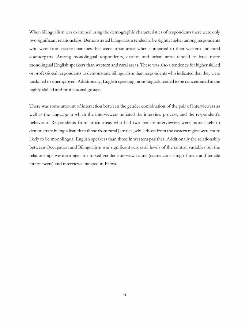
When bilingualism was examined using the demographic characteristics of respondents there were only

two significant relationships. Demonstrated bilingualism tended to be slightly higher among respondents

who were from eastern parishes that were urban areas when compared to their western and rural

counterparts. Among monolingual respondents, eastern and urban areas tended to have more

monolingual English speakers than western and rural areas. There was also a tendency for higher skilled

or professional respondents to demonstrate bilingualism than respondents who indicated that they were

unskilled or unemployed. Additionally, English speaking monolinguals tended to be concentrated in the

highly skilled and professional groups.

There was some amount of interaction between the gender combination of the pair of interviewers as

well as the language in which the interviewers initiated the interview process, and the respondent’s

behaviour. Respondents from urban areas who had two female interviewers were more likely to

demonstrate bilingualism than those from rural Jamaica, while those from the eastern region were more

likely to be monolingual English speakers than those in western parishes. Additionally the relationship

between Occupation and Bilingualism was significant across all levels of the control variables but the

relationships were stronger for mixed gender interview teams (teams consisting of male and female

interviewers) and interviews initiated in Patwa.

7

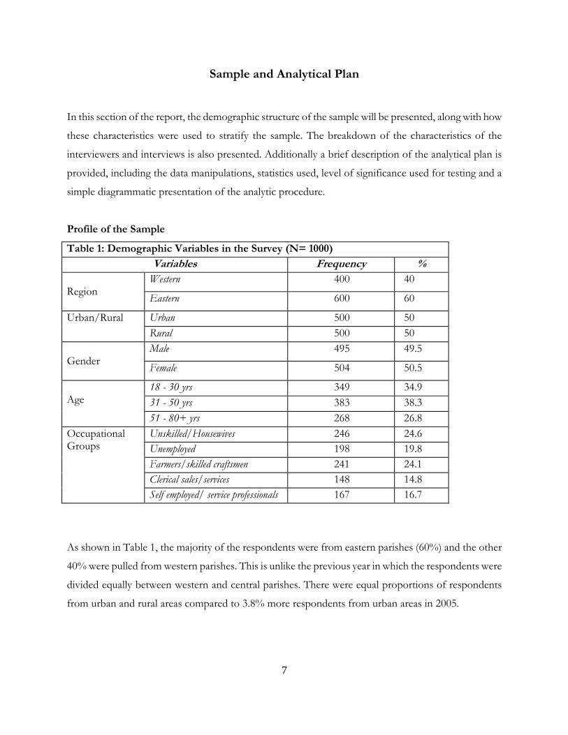
Sample and Analytical Plan

In this section of the report, the demographic structure of the sample will be presented, along with how

these characteristics were used to stratify the sample. The breakdown of the characteristics of the

interviewers and interviews is also presented. Additionally a brief description of the analytical plan is

provided, including the data manipulations, statistics used, level of significance used for testing and a

simple diagrammatic presentation of the analytic procedure.

Profile of the Sample

Table 1: Demographic Variables in the Survey (N= 1000)

Variables Frequency %

Region

Western 400 40

Eastern 600 60

Urban/Rural

Urban 500 50

Rural 500 50

Gender

Male 495 49.5

Female 504 50.5

Age

18 - 30 yrs 349 34.9

31 - 50 yrs 383 38.3

51 - 80+ yrs 268 26.8

Occupational Groups

Unskilled/Housewives 246 24.6

Unemployed 198 19.8

Farmers/skilled craftsmen 241 24.1

Clerical sales/services 148 14.8

Self employed/ service professionals 167 16.7

As shown in Table 1, the majority of the respondents were from eastern parishes (60%) and the other

40% were pulled from western parishes. This is unlike the previous year in which the respondents were

divided equally between western and central parishes. There were equal proportions of respondents

from urban and rural areas compared to 3.8% more respondents from urban areas in 2005.

8

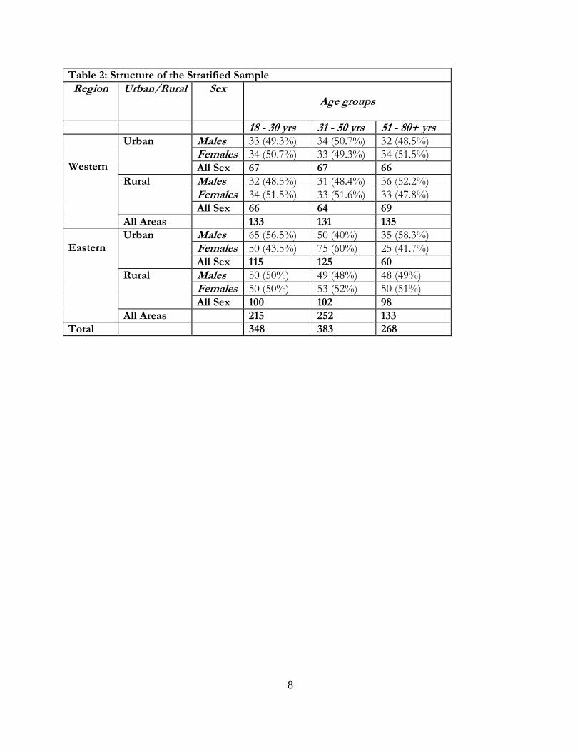
Table 2: Structure of the Stratified Sample Region Urban/Rural Sex

Age groups

18 - 30 yrs 31 - 50 yrs 51 - 80+ yrs Western

Urban

Males 33 (49.3%) 34 (50.7%) 32 (48.5%) Females 34 (50.7%) 33 (49.3%) 34 (51.5%) All Sex 67 67 66

Rural

Males 32 (48.5%) 31 (48.4%) 36 (52.2%) Females 34 (51.5%) 33 (51.6%) 33 (47.8%) All Sex 66 64 69

All Areas 133 131 135 Eastern

Urban

Males 65 (56.5%) 50 (40%) 35 (58.3%) Females 50 (43.5%) 75 (60%) 25 (41.7%) All Sex 115 125 60

Rural

Males 50 (50%) 49 (48%) 48 (49%) Females 50 (50%) 53 (52%) 50 (51%) All Sex 100 102 98

All Areas 215 252 133 Total 348 383 268

9

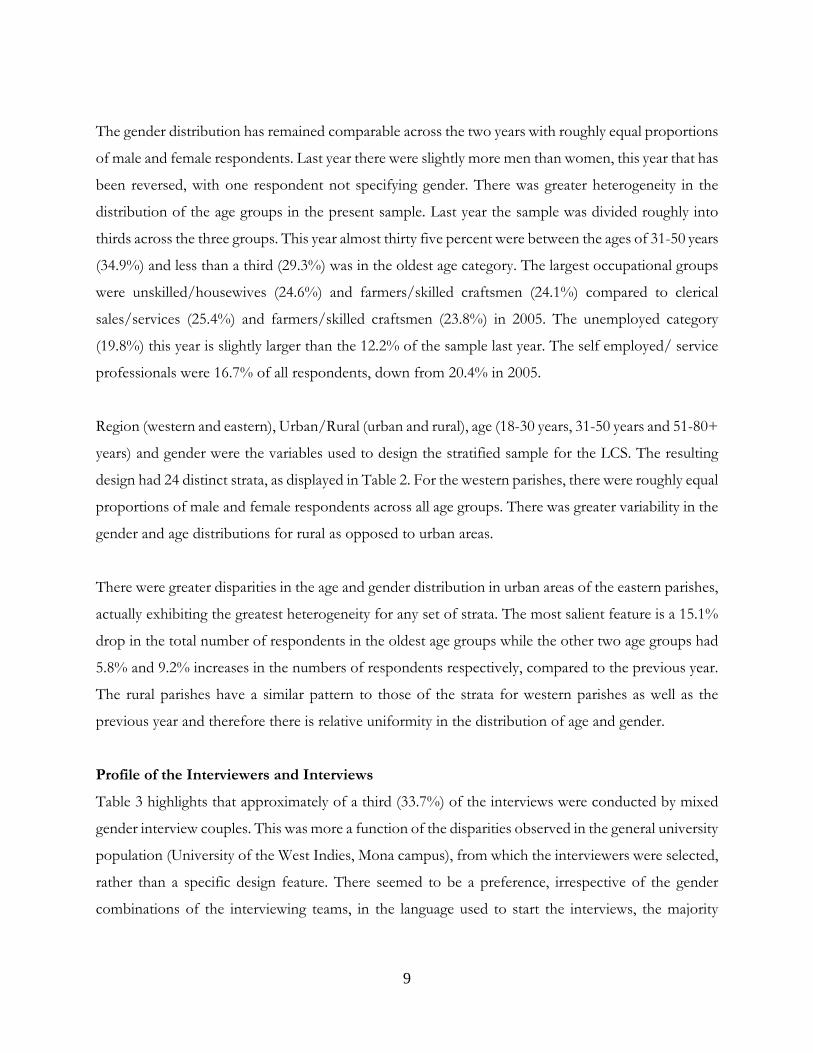
The gender distribution has remained comparable across the two years with roughly equal proportions

of male and female respondents. Last year there were slightly more men than women, this year that has

been reversed, with one respondent not specifying gender. There was greater heterogeneity in the

distribution of the age groups in the present sample. Last year the sample was divided roughly into

thirds across the three groups. This year almost thirty five percent were between the ages of 31-50 years

(34.9%) and less than a third (29.3%) was in the oldest age category. The largest occupational groups

were unskilled/housewives (24.6%) and farmers/skilled craftsmen (24.1%) compared to clerical

sales/services (25.4%) and farmers/skilled craftsmen (23.8%) in 2005. The unemployed category

(19.8%) this year is slightly larger than the 12.2% of the sample last year. The self employed/ service

professionals were 16.7% of all respondents, down from 20.4% in 2005.

Region (western and eastern), Urban/Rural (urban and rural), age (18-30 years, 31-50 years and 51-80+

years) and gender were the variables used to design the stratified sample for the LCS. The resulting

design had 24 distinct strata, as displayed in Table 2. For the western parishes, there were roughly equal

proportions of male and female respondents across all age groups. There was greater variability in the

gender and age distributions for rural as opposed to urban areas.

There were greater disparities in the age and gender distribution in urban areas of the eastern parishes,

actually exhibiting the greatest heterogeneity for any set of strata. The most salient feature is a 15.1%

drop in the total number of respondents in the oldest age groups while the other two age groups had

5.8% and 9.2% increases in the numbers of respondents respectively, compared to the previous year.

The rural parishes have a similar pattern to those of the strata for western parishes as well as the

previous year and therefore there is relative uniformity in the distribution of age and gender.

Profile of the Interviewers and Interviews

Table 3 highlights that approximately of a third (33.7%) of the interviews were conducted by mixed

gender interview couples. This was more a function of the disparities observed in the general university

population (University of the West Indies, Mona campus), from which the interviewers were selected,

rather than a specific design feature. There seemed to be a preference, irrespective of the gender

combinations of the interviewing teams, in the language used to start the interviews, the majority

10

(53.2%) of which was started in Patwa. This roughly translates into six percent more interviews initiated

using Patwa.

Data Analysis and Manipulation

The data was analyzed using the Statistical Package of the Social Sciences (SPSS). The variables used in

the analysis were categorical, therefore the Chi-square statistic was used to examine the bivariate

relationships. Additionally, all relationships were tested using a significance level of five percent (5%).

The implication of this is that the maximum probability of the risk of making a Type I error was 0.05.

Therefore all displayed significance levels that were below 0.05 were deemed to be statistically significant

(any significance level that was exactly, as well as when rounded, equal to or greater than 0.05, was

considered to be statistically insignificant).

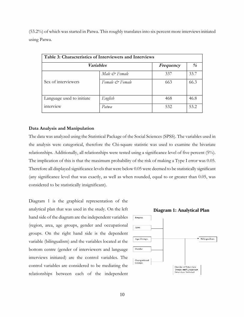
Diagram 1 is the graphical representation of the

analytical plan that was used in the study. On the left

hand side of the diagram are the independent variables

(region, area, age groups, gender and occupational

groups. On the right hand side is the dependent

variable (bilingualism) and the variables located at the

bottom centre (gender of interviewers and language

interviews initiated) are the control variables. The

control variables are considered to be mediating the

relationships between each of the independent

Table 3: Characteristics of Interviewers and Interviews

Variables Frequency %

Sex of interviewers

Male & Female 337 33.7

Female & Female 663 66.3

Language used to initiate

interview

English 468 46.8

Patwa 532 53.2

Diagram 1: Analytical Plan

11

variables and the dependent variable. These relationships were assessed to identify potential

confounding relationships. Generally, only the relationships that were statistically significant were

reported and discussed.

There are two notable variable modifications that were made for the analysis. The variable used to

measure occupation groups was created by recoding the variable OCCUPAT. The original variable had

a total of nine categories was simply regrouped into five (which can be seen in Table 1 above).

Specifically, the categories labeled self employed/service professionals, farmers/skilled craftsmen and

unemployed were created by collapsing as the names suggest self employed professionals with service

professional, farmers with skilled crafts men and unemployed consisted of students, retired and

unemployed respondents. This was done primarily to achieve parity with what was done in the previous

year as well as to subsume categories into larger operational categories for occupational groups.

The variable BILINGUALISM was a ‘proxy variable’ used to measure language competence, was

created by the summation of three variables; Q8 (Language at scenario – Jamaican or English), Q9

(Language at prompt – Jamaican or English) and Q10 (Language at debrief – Jamaican or English).

These variables were first recoded, weighting the values of each variable to ensure that each

characteristic represented by these variables would be clearly distinguishable when summed. After the

creation of the proxy variable it was recoded into the three groups displayed in Table 4 below. This

seemingly elaborate undertaking was done because each variable (Q8, Q9 and Q10) measured different

aspects of the process used to measure bilingualism. Therefore no one variable was suitable as an

adequate measure of bilingualism. This then necessitated the combination of all three to develop an

accurate (as was possible) measure of bilingualism.

12

Data Presentation

Bilingualism

Table 4: Bilingualism Variable Frequency %

Monolingualism

English 171 17.1

Patwa 365 36.5

Bilingualism Demonstrated Bilingualism 464 46.4

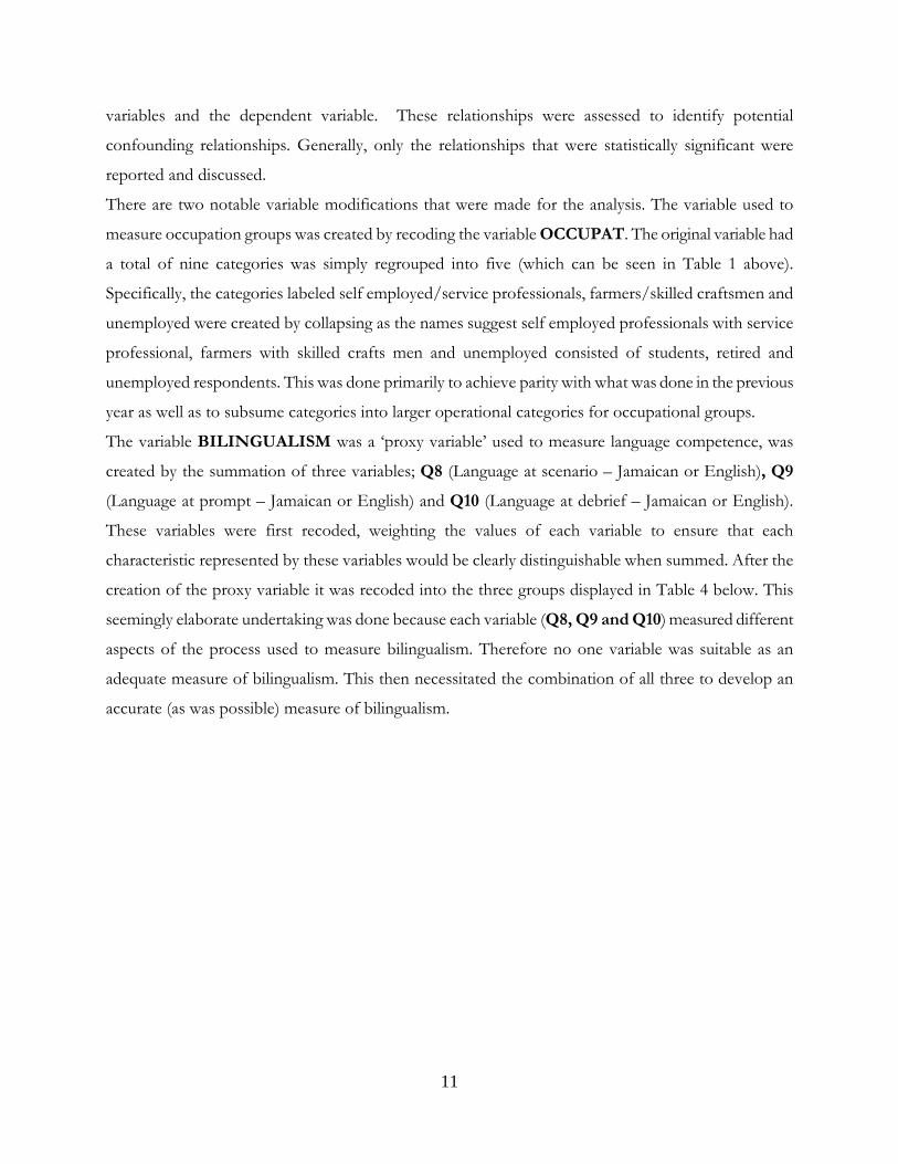
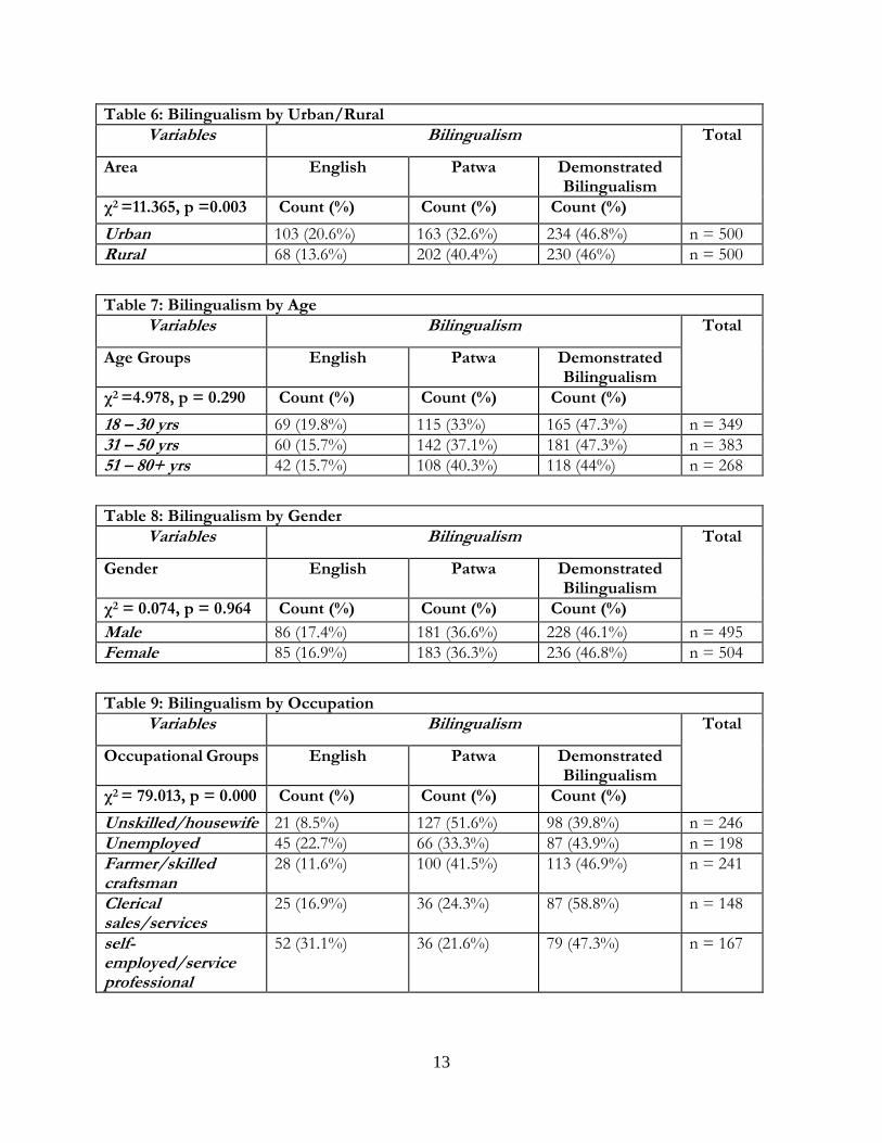
From Table 4, it can be seen that 46.4% of the respondents demonstrated bilingualism. Less than 20%

of the sample were monolinguals that spoke only English and just over a third (36.5%) of the

respondents were Patwa speaking mono-linguals (either because they did not speak both languages

during the interview or told the interviewers that they were capable of doing so but did not demonstrate

competence in both).

Independent Variables: Region, Urban/Rural, Age, Gender, Occupation

Table 5-9 present the results of the chi-square analysis, examining the relationships between

bilingualism and region, Urban/Rural, age, gender and occupation. Only three of relationships were

found to be statistically significant, namely Region, Urban/Rural and Occupational Groups with

Bilingualism.

Table 5: Bilingualism by Region Variables Bilingualism

Total

Region English Patwa Demonstrated Bilingualism

χ2 = 7.998, p = 0.018 Count (%) Count (%) Count (%) Western 54 (13.5%) 162 (40.5%) 184 (46%) n = 400 Eastern 117 (19.5%) 203 (33.8%) 280 (46.7%) n = 600

13

Table 6: Bilingualism by Urban/Rural Variables Bilingualism Total

Area English Patwa Demonstrated Bilingualism

χ2 =11.365, p =0.003 Count (%) Count (%) Count (%)

Urban 103 (20.6%) 163 (32.6%) 234 (46.8%) n = 500 Rural 68 (13.6%) 202 (40.4%) 230 (46%) n = 500

Table 7: Bilingualism by Age Variables Bilingualism Total

Age Groups English Patwa Demonstrated Bilingualism

χ2 =4.978, p = 0.290 Count (%) Count (%) Count (%)

18 – 30 yrs 69 (19.8%) 115 (33%) 165 (47.3%) n = 349 31 – 50 yrs 60 (15.7%) 142 (37.1%) 181 (47.3%) n = 383 51 – 80+ yrs 42 (15.7%) 108 (40.3%) 118 (44%) n = 268

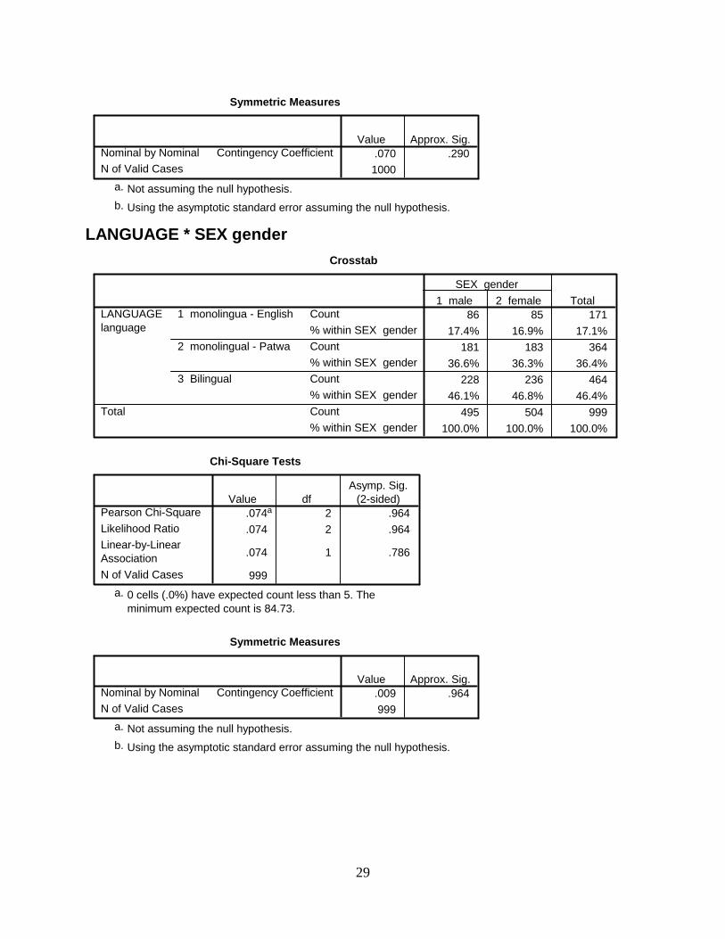
Table 8: Bilingualism by Gender Variables Bilingualism Total

Gender English Patwa Demonstrated Bilingualism

χ2 = 0.074, p = 0.964 Count (%) Count (%) Count (%)

Male 86 (17.4%) 181 (36.6%) 228 (46.1%) n = 495 Female 85 (16.9%) 183 (36.3%) 236 (46.8%) n = 504

Table 9: Bilingualism by Occupation Variables Bilingualism Total

Occupational Groups English Patwa Demonstrated Bilingualism

χ2 = 79.013, p = 0.000 Count (%) Count (%) Count (%)

Unskilled/housewife 21 (8.5%) 127 (51.6%) 98 (39.8%) n = 246 Unemployed 45 (22.7%) 66 (33.3%) 87 (43.9%) n = 198 Farmer/skilled craftsman

28 (11.6%) 100 (41.5%) 113 (46.9%) n = 241

Clerical sales/services

25 (16.9%) 36 (24.3%) 87 (58.8%) n = 148

self-employed/service professional

52 (31.1%) 36 (21.6%) 79 (47.3%) n = 167

14

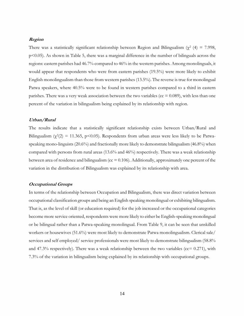
Region

There was a statistically significant relationship between Region and Bilingualism (χ2 (4) = 7.998,

p<0.05). As shown in Table 5, there was a marginal difference in the number of bilinguals across the

regions: eastern parishes had 46.7% compared to 46% in the western parishes. Among monolinguals, it

would appear that respondents who were from eastern parishes (19.5%) were more likely to exhibit

English monolingualism than those from western parishes (13.5%). The reverse is true for monolingual

Patwa speakers, where 40.5% were to be found in western parishes compared to a third in eastern

parishes. There was a very weak association between the two variables (cc = 0.089), with less than one

percent of the variation in bilingualism being explained by its relationship with region.

Urban/Rural

The results indicate that a statistically significant relationship exists between Urban/Rural and

Bilingualism (χ2(2) = 11.365, p<0.05). Respondents from urban areas were less likely to be Patwa-

speaking mono-linguists (20.6%) and fractionally more likely to demonstrate bilingualism (46.8%) when

compared with persons from rural areas (13.6% and 46%) respectively. There was a weak relationship

between area of residence and bilingualism (cc = 0.106). Additionally, approximately one percent of the

variation in the distribution of Bilingualism was explained by its relationship with area.

Occupational Groups

In terms of the relationship between Occupation and Bilingualism, there was direct variation between

occupational classification groups and being an English speaking monolingual or exhibiting bilingualism.

That is, as the level of skill (or education required) for the job increased or the occupational categories

become more service oriented, respondents were more likely to either be English-speaking monolingual

or be bilingual rather than a Patwa-speaking monolingual. From Table 9, it can be seen that unskilled

workers or housewives (51.6%) were most likely to demonstrate Patwa monolingualism. Clerical sale/

services and self employed/ service professionals were most likely to demonstrate bilingualism (58.8%

and 47.3% respectively). There was a weak relationship between the two variables (cc= 0.271), with

7.3% of the variation in bilingualism being explained by its relationship with occupational groups.

15

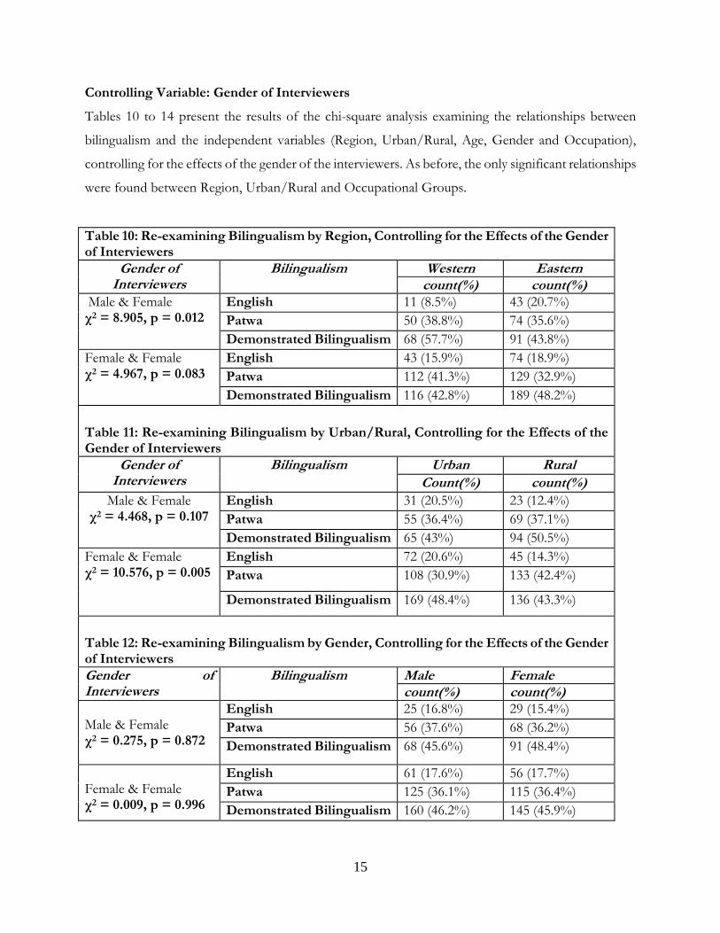
Controlling Variable: Gender of Interviewers

Tables 10 to 14 present the results of the chi-square analysis examining the relationships between

bilingualism and the independent variables (Region, Urban/Rural, Age, Gender and Occupation),

controlling for the effects of the gender of the interviewers. As before, the only significant relationships

were found between Region, Urban/Rural and Occupational Groups.

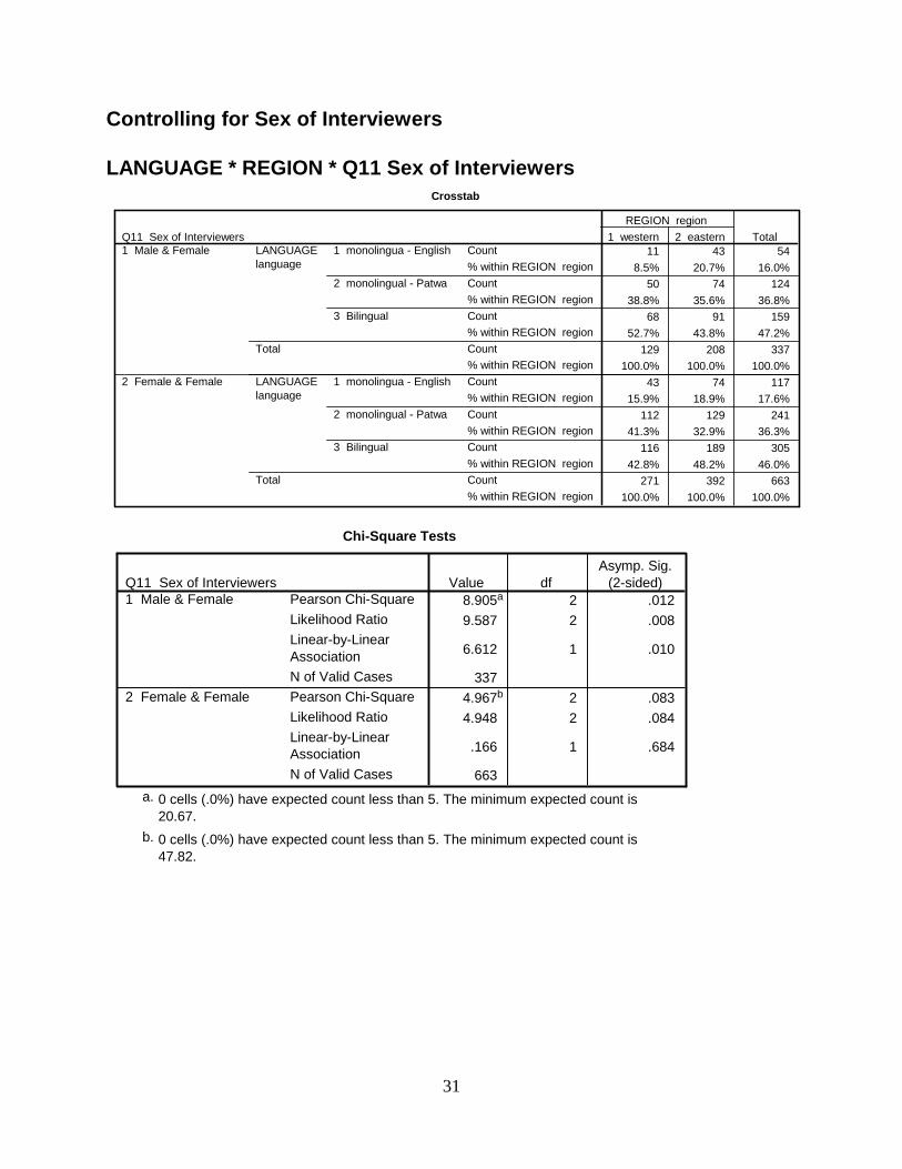
Table 10: Re-examining Bilingualism by Region, Controlling for the Effects of the Gender of Interviewers


Bilingualism Western Eastern count(%) count(%)

Male & Female χ2 = 8.905, p = 0.012

English 11 (8.5%) 43 (20.7%)

Patwa 50 (38.8%) 74 (35.6%)

Demonstrated Bilingualism 68 (57.7%) 91 (43.8%)

Female & Female χ2 = 4.967, p = 0.083

English 43 (15.9%) 74 (18.9%)

Patwa 112 (41.3%) 129 (32.9%)


Table 11: Re-examining Bilingualism by Urban/Rural, Controlling for the Effects of the Gender of Interviewers


Bilingualism Urban Rural

Count(%) count(%)

Male & Female χ2 = 4.468, p = 0.107

English 31 (20.5%) 23 (12.4%)

Patwa 55 (36.4%) 69 (37.1%)

Demonstrated Bilingualism 65 (43%) 94 (50.5%)

Female & Female χ2 = 10.576, p = 0.005

English 72 (20.6%) 45 (14.3%)

Patwa 108 (30.9%) 133 (42.4%)


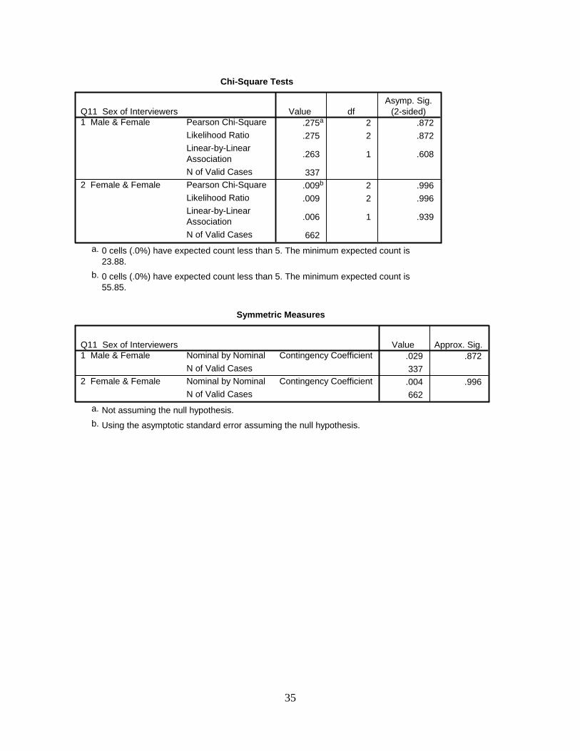
Table 12: Re-examining Bilingualism by Gender, Controlling for the Effects of the Gender of Interviewers Gender of Interviewers

Bilingualism Male Female count(%) count(%)

Male & Female χ2 = 0.275, p = 0.872

English 25 (16.8%) 29 (15.4%)

Patwa 56 (37.6%) 68 (36.2%)


Female & Female χ2 = 0.009, p = 0.996

English 61 (17.6%) 56 (17.7%)

Patwa 125 (36.1%) 115 (36.4%)


16

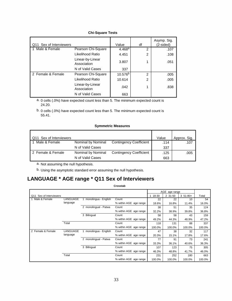
Table 13: Re-examining Bilingualism by Age, Controlling for the Effects of the Gender of Interviewers Gender of Interviewers

Age Groups English Patwa Demonstrated Bilingualism

Male & Female

18 - 30yrs 22 (18.6%) 38 (32.2%) 58 (49.2%)

χ2 = 3.182, p = 0.528

31 - 50yrs 22 (16.8%) 51 (38.9%) 58 (44.3%)

51 - 80+ yrs 10 (11.4%) 35 (39.8%) 43 (48.9%)

Female & Female χ2 = 4.527, p = 0.339

18 - 30yrs 47 (20.3%) 77 (33.3%) 107 (46.3%)

31 - 50yrs 38 (15.1%) 91 (36.1%) 123 (48.8%)

51 - 80+ yrs 32 (17.8%) 73 (40.6%) 75 (41.7%)

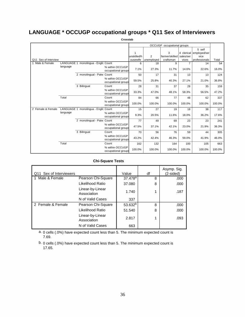
Table 14: Re-examining Bilingualism by Occupation, Controlling for the Effects of the Gender of Interviewers Gender of Interviewers

Occupational Groups English Patwa Demonstrated Bilingualism

Male & Female χ2 = 37.478, p = 0.000

Unskilled/housewife 6 (7.1%) 50 (59.5%) 28 (33.3%) Unemployed 18 (27.3%) 17 (25.8%) 31 (47%)

Farmer/skilled craftsman

9 (11.7%) 31 (40.3%) 37 (48.1%)

Clerical sales/services 7 (14.6%) 13 (27.1%) 28 (58.3%) self-employed/service professional

14 (22.6%) 13 (21.0%) 35 (56.5%)

Female & Female χ2 = 53.632 p = 0.000

Unskilled/housewife 15 (9.3%) 77 (47.5%) 70 (43.2%) Unemployed 27 (20.5%) 49 (37.1%) 56 (42.4%)


19 (11.6%) 69 (42.1%) 76 (46.3%)

Clerical sales/services 18 (18%) 23 (23%) 59 (59%) self-employed/service professional

38 (36.2%) 23 (21.9%) 44 (41.9%)

Region

From Table 10, the relationship between Region and Bilingualism is significant for respondents who

where interviewed by mixed gender interview teams (χ2 (2) = 8.905, p<0.05). The nature of this

relationship is similar to what was previously described for the test between both variables without the

17

control variable. Specifically, respondents from eastern parishes are more like to be monolingual-

English speakers (20.7%) than those from western parishes (8.5%). However there was one notable

exception, there were more bilinguals in the western region than in the east (52.7% compared to 43.8%).

There was a marked increase in the strength of the relation (from cc=0.086 to cc = 0.160) which in turn

increased the explained variation from approximately 0.7% to approximately 2.5% of the variation in

bilingualism. This would suggest that the relationship is true of those respondents interviewed by mixed

gender interviewers rather than those that had only female interviewers.

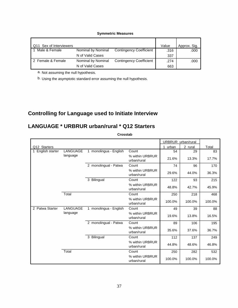
Urban/Rural

As before when looking solely on area, the results indicate that there is a statistically significant

relationship between Urban/Rural and Bilingualism (χ2 (2) = 11.365, p<0.05). However, this time it is

only true for the interviews conducted by interview teams that had only female interviewers. The

general nature of the relationship is also the same but the pattern is more distinctive. As seen in Table

11, respondents from urban areas were more likely to be bilinguals (48.4%) when compared with

respondents from rural areas (43.3%). If they are monolinguals, they are more likely to speak English

(20.6%) compared to their rural counterparts (14.3%). The strength of the relationship increased, but

still remained weak (cc = 0.114). While this does point to an interaction of some sort between the

gender of the interviewers and the behaviour of respondents, it is important to note that only a third of

these interviews were conducted by mixed gender interview teams. Therefore it cannot conclusively be

determined that such an interaction is indeed a true reflection of the effect of interviewer gender,

particularly since there were no single sex male interview teams.

Occupational Groups

As seen in Table 14, the results obtained for the relationship between Occupational Groups and

Bilingualism is similar to what was obtained before and is significant for both types of interview couples.

This would indicate that the relationship is true generally for the sample and the gender of the

interviewers had little effect on this relationship (although the relationship is stronger for mixed gender

interview teams). As with Urban/Rural, the pattern of interaction between the independent and

dependent variable is much more delineated. The pattern indicates that unskilled/ housewives, if

monolingual, are more likely to be Patwa speakers than were respondents in the clerical or professional

categories. Overall, unskilled and housewives are also less likely to be bilingual than their counterparts in

the clerical or professional categories.

18

Even though the relation was significant for both types of interview teams, the fact that the relationship

was stronger for mixed gender interview teams does indicate some level of interaction. Approximately

10% of the variation in bilingualism is explained by its relationship with occupation for mixed gender

interview teams, which is two percent (2%) more than what is explained by the same relationship for all

female teams. It is important however to note that while this reinforces the idea of the confounding

effect that the gender of the interview teams had on the relationship, without that third group (single sex

male interview teams) it is not possible to fully understand the nature of this interaction.

Controlling Variable: Language Used to Initiate Interview

Tables 15 to 19 present the results of the chi-square analysis examining the relationships between

bilingualism and the independent variables (region, Urban/Rural, Age, Gender and Occupation)

controlling for the effects of the language used to initiate the interviews. The variables Region,

Urban/Rural, Age and Occupational groups were found to be significantly related to Bilingualism.

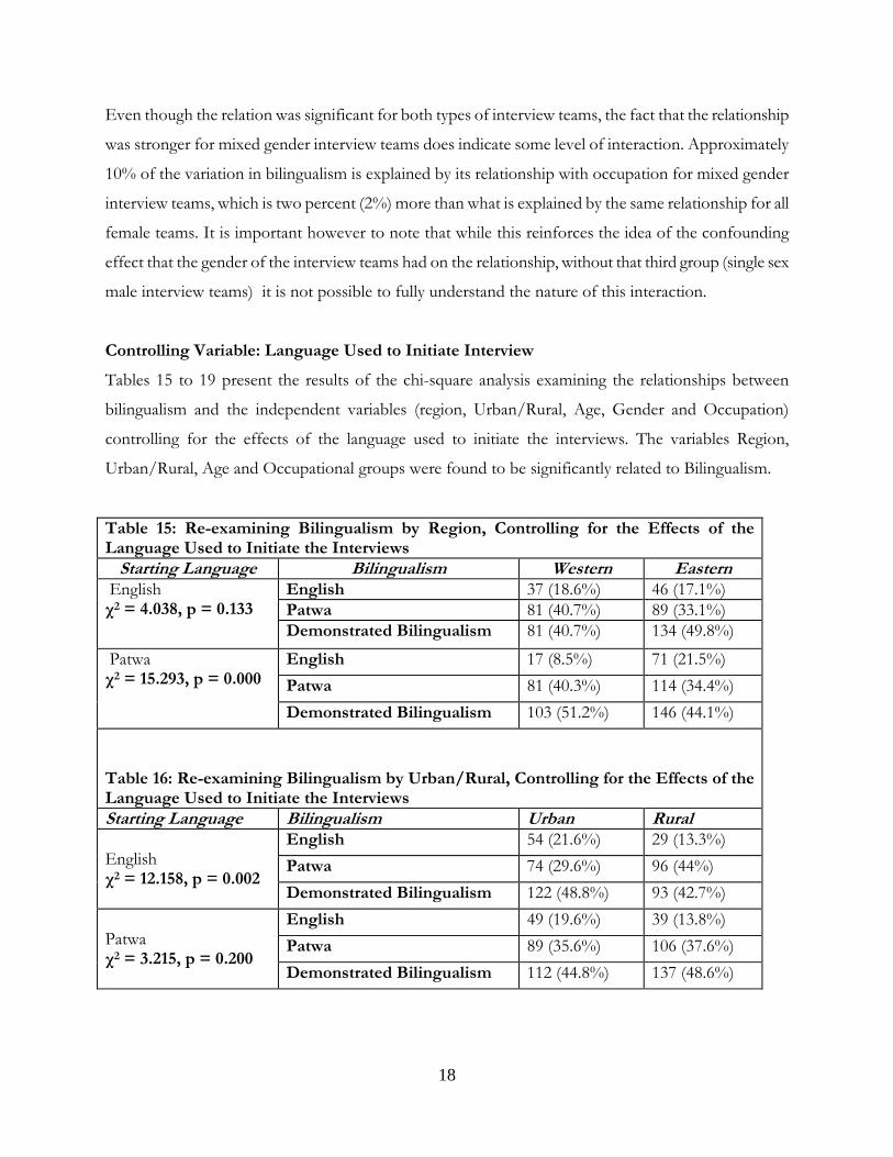
Table 15: Re-examining Bilingualism by Region, Controlling for the Effects of the Language Used to Initiate the Interviews Starting Language Bilingualism Western Eastern

English χ2 = 4.038, p = 0.133

English 37 (18.6%) 46 (17.1%) Patwa 81 (40.7%) 89 (33.1%) Demonstrated Bilingualism 81 (40.7%) 134 (49.8%)

Patwa χ2 = 15.293, p = 0.000

English 17 (8.5%) 71 (21.5%)

Patwa 81 (40.3%) 114 (34.4%)


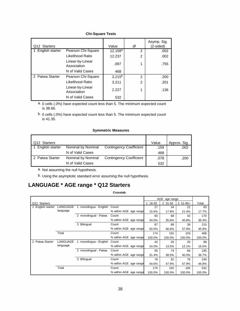
Table 16: Re-examining Bilingualism by Urban/Rural, Controlling for the Effects of the Language Used to Initiate the Interviews Starting Language Bilingualism Urban Rural English χ2 = 12.158, p = 0.002

English 54 (21.6%) 29 (13.3%)

Patwa 74 (29.6%) 96 (44%)


Patwa χ2 = 3.215, p = 0.200

English 49 (19.6%) 39 (13.8%)

Patwa 89 (35.6%) 106 (37.6%)


19

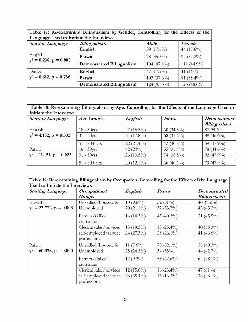
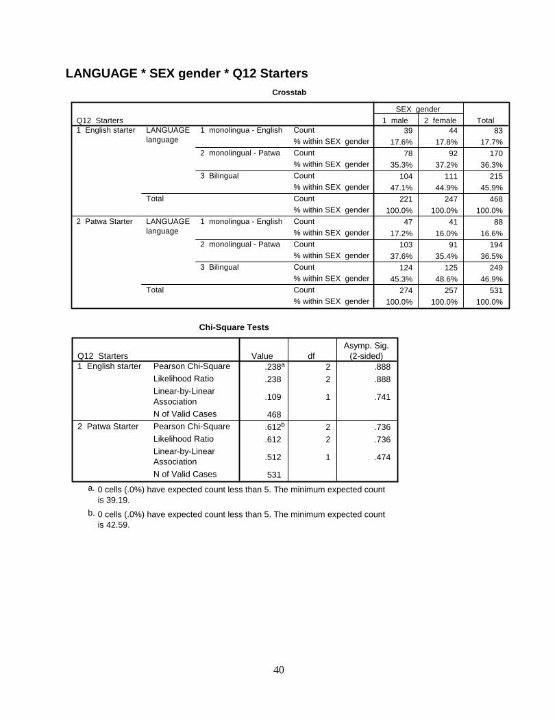
Table 17: Re-examining Bilingualism by Gender, Controlling for the Effects of the Language Used to Initiate the Interviews Starting Language Bilingualism Male Female English χ2 = 0.238, p = 0.888

English 39 (17.6%) 44 (17.8%)

Patwa 78 (35.3%) 92 (37.2%)


Patwa χ2 = 0.612, p = 0.736

English 47 (17.2%) 41 (16%)

Patwa 103 (37.6%) 91 (35.4%)


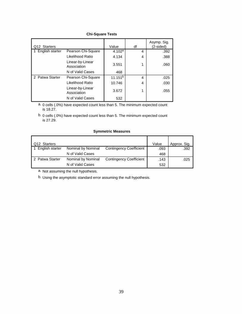
Table 18: Re-examining Bilingualism by Age, Controlling for the Effects of the Language Used to Initiate the Interviews Starting Language Age Groups English Patwa Demonstrated

Bilingualism English χ2 = 4.102, p = 0.392

18 - 30yrs 27 (15.5%) 60 (34.5%) 87 (50%) 31 - 50yrs 34 (17.8%) 68 (35.6%) 89 (46.6%)

51 - 80+ yrs 22 (21.4%) 42 (40.8%) 39 (37.9%) Patwa χ2 = 11.151, p = 0.025

18 - 30yrs 42 (24%) 55 (31.4%) 78 (44.6%) 31 - 50yrs 26 (13.5%) 74 (38.5%) 92 (47.9%)

51 - 80+ yrs 20 (12.1%) 66 (40.1%) 79 (47.9%) Table 19: Re-examining Bilingualism by Occupation, Controlling for the Effects of the Language Used to Initiate the Interviews Starting Language Occupational

Groups English Patwa Demonstrated

Bilingualism English χ2 = 23.722, p = 0.003

Unskilled/housewife 10 (9.8%) 52 (51%) 40 39.2%) Unemployed 20 (21.1%) 32 (33.7%) 43 (45.3%)


16 (14.3%) 45 (40.2%) 51 (45.5%)

Clerical sales/services 13 (18.3%) 18 (25.4%) 40 (56.3%) self-employed/service professional

24 (27.3%) 23 (26.1%) 41 (46.6%)

Patwa χ2 = 60.378, p = 0.000

Unskilled/housewife 11 (7.6%) 75 (52.1%) 58 (40.3%) Unemployed 25 (24.3%) 34 (33%) 44 (42.7%)


12 (9.3%) 55 (42.6%) 62 (48.1%)

Clerical sales/services 12 (15.6%) 18 (23.4%) 47 (61%) self-employed/service professional

28 (35.4%) 13 (16.5%) 38 (48.1%)

20

Region

There was a significant relationship (χ2 (2) = 15.293, p<0.05) between Region and Bilingualism but only

for those interviews that were initiated in Patwa (Table 15). As previously highlighted, respondents from

western parishes were more likely to be bilingual (51.2%) and if they were bilingual they were less likely

to be English speakers (8.5% compared to 21.5%). This relationship was weak accounting for less than

three percent of the variation in bilingualism.

Urban/Rural

According to the results from Table 16, there is a significant relationship between Urban/Rural and

Bilingualism but it is only significant for interviews that were initiated in English. In keeping with the

general trend for this relationship (see Table 10), urban respondents are more likely to be bilinguals

(48.8%) than those from rural areas (42.7%). Similar to what was found when the gender of the

interview teams was used as a control for the amount of variation in the relationship increased to

approximately 2.5%. This suggests that this relationship is mediated both by the gender or the interview

teams and the language that was used to initiate the interviews. It is possible that male-female interview

teams tended to start interviews in English more so than Patwa.

Age

There was a significant relationship between Age and Bilingualism when the language used to initiate the

interview was held constant (Table 18). The relationship was true for respondents that started the

interview process with a scenario presented in Patwa. Older respondents (47.9%) were more likely to

report bilingualism than younger respondents (44.36%). However among those respondents that were

monolinguals, younger respondents were more likely to be English speakers (24%) compared to their

older counterparts who were Patwa speakers (66%). This relationship was weak explaining two percent

of the variation in bilingualism.

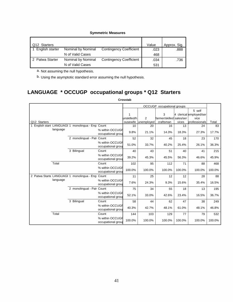
Occupational Groups

From Table 19, irrespective of the language that the interview was started there was a relationship

between Occupational Groups and Bilingualism. While the same general trend could be observed in the

relationship (monolingual respondents tended to be less skilled than bilinguals and among monolinguals

monolingual English speakers tended to be from the higher skilled groups), there was a stronger

association between the variables for those interviews that were initiated using Patwa. On the one hand,

21

under this controlled condition (interviews started with Patwa), occupational group accounted for 10.2%

of the variation in Bilingualism. On the other hand, for those interviews initiated in English

occupational groups accounted for only 4.8%. Altogether this would indicate that the relationship

between occupational groups and Bilingualism is mediated by the language the interviewers used to start

the interview process.

Conclusion

There were significant relationships for three of the five variables: Region, Urban/Rural and

Occupational group. Individuals that resided in eastern parishes tended to be bilingual or, if

monolingual, were more likely to be English speakers. Urban area respondents/residents were more

likely to be bilingual than those who were from rural areas. However, most English speaking

monolinguals were to be found in urban areas. Respondents who classified themselves as clerical sales/

services or the self employed/service professionals were more likely to be bilingual than those who were

unskilled/housewives or unemployed. Within the occupational groups those who were monolingual

Patwa speakers were concentrated in the lower skilled groups.

When the analytical model was re-examined holding the gender of the interviewers constant as well as

the language that was used to initiate the interviews, the same variables (Region, Urban/Rural and

Occupational groups) were found to be significant. (Age was significant but only when the second

control variable, language used to initiate interview, was used) All three relationships were affected by

both control variables, which indicated potential methodological confounds. Specifically, the

relationship between Age and bilingualism was only significant for those interviews that were initiated

using Patwa. The relationship between bilingualism and Region was significant for male-female

interview teams but not for all female teams and those interviews that were initiated using Patwa. The

relationship between Urban/Rural and bilingualism was only significant for female interview couples

and interviews imitated in English. A possible explanation for this is that male-female interview teams

were more likely to start interviews using Patwa while all female teams were more likely to start using

English (although they could be unrelated incidents). The relationship between Occupational Groups

and Bilingualism was significant for the sample irrespective of whether respondents were interviewed by

a mixed gender or all female teams or the interview was started with Patwa or English. It most be noted

22

however that the relationship was stronger for mixed gender interview teams and interviews that were

initiated using Patwa.

23

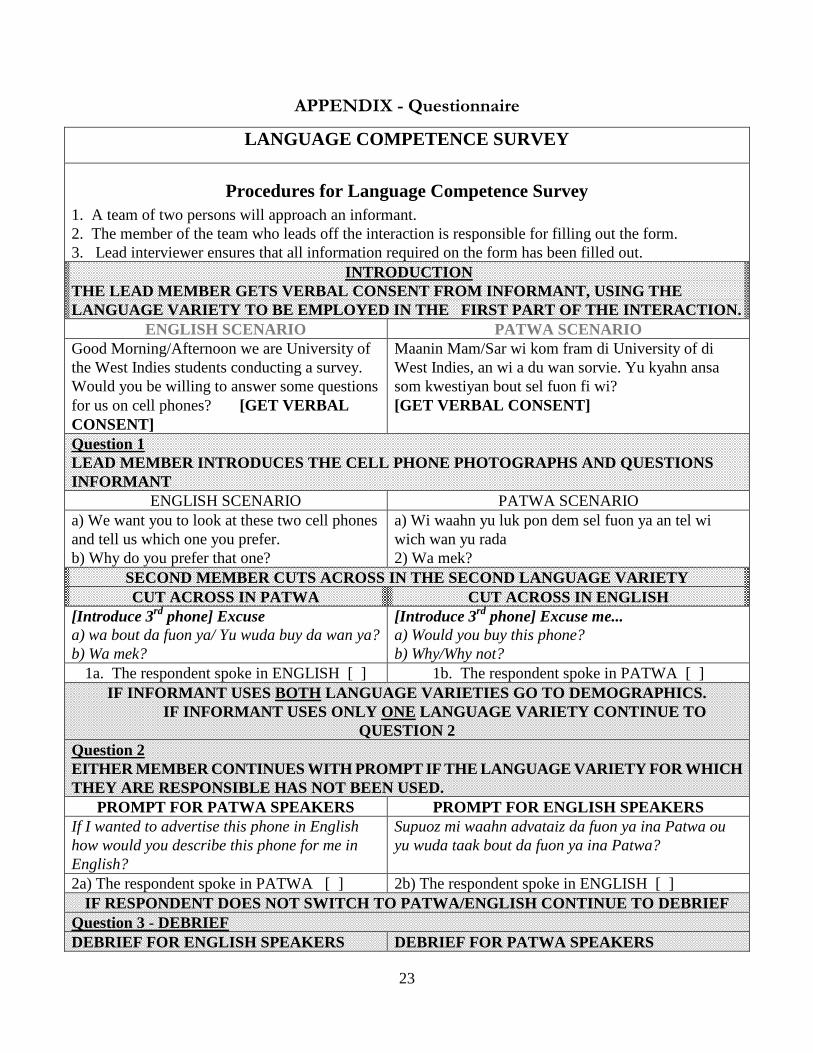
APPENDIX - Questionnaire

LANGUAGE COMPETENCE SURVEY

Procedures for Language Competence Survey 1. A team of two persons will approach an informant. 2. The member of the team who leads off the interaction is responsible for filling out the form. 3. Lead interviewer ensures that all information required on the form has been filled out.

INTRODUCTION THE LEAD MEMBER GETS VERBAL CONSENT FROM INFORMANT, USING THE LANGUAGE VARIETY TO BE EMPLOYED IN THE FIRST PART OF THE INTERACTION.

ENGLISH SCENARIO PATWA SCENARIO Good Morning/Afternoon we are University of the West Indies students conducting a survey. Would you be willing to answer some questions for us on cell phones? [GET VERBAL CONSENT]

Maanin Mam/Sar wi kom fram di University of di West Indies, an wi a du wan sorvie. Yu kyahn ansa som kwestiyan bout sel fuon fi wi? [GET VERBAL CONSENT]

Question 1 LEAD MEMBER INTRODUCES THE CELL PHONE PHOTOGRAPHS AND QUESTIONS INFORMANT

ENGLISH SCENARIO PATWA SCENARIO a) We want you to look at these two cell phones and tell us which one you prefer. b) Why do you prefer that one?

a) Wi waahn yu luk pon dem sel fuon ya an tel wi wich wan yu rada 2) Wa mek?

SECOND MEMBER CUTS ACROSS IN THE SECOND LANGUAGE VARIETY CUT ACROSS IN PATWA CUT ACROSS IN ENGLISH

[Introduce 3rd phone] Excuse a) wa bout da fuon ya/ Yu wuda buy da wan ya? b) Wa mek?

[Introduce 3rd phone] Excuse me... a) Would you buy this phone? b) Why/Why not?

1a. The respondent spoke in ENGLISH [ ] 1b. The respondent spoke in PATWA [ ] IF INFORMANT USES BOTH LANGUAGE VARIETIES GO TO DEMOGRAPHICS. IF INFORMANT USES ONLY ONE LANGUAGE VARIETY CONTINUE TO

QUESTION 2 Question 2 EITHER MEMBER CONTINUES WITH PROMPT IF THE LANGUAGE VARIETY FOR WHICH THEY ARE RESPONSIBLE HAS NOT BEEN USED.

PROMPT FOR PATWA SPEAKERS PROMPT FOR ENGLISH SPEAKERS If I wanted to advertise this phone in English how would you describe this phone for me in English?

Supuoz mi waahn advataiz da fuon ya ina Patwa ou yu wuda taak bout da fuon ya ina Patwa?

2a) The respondent spoke in PATWA [ ] 2b) The respondent spoke in ENGLISH [ ] IF RESPONDENT DOES NOT SWITCH TO PATWA/ENGLISH CONTINUE TO DEBRIEF

Question 3 - DEBRIEF DEBRIEF FOR ENGLISH SPEAKERS DEBRIEF FOR PATWA SPEAKERS

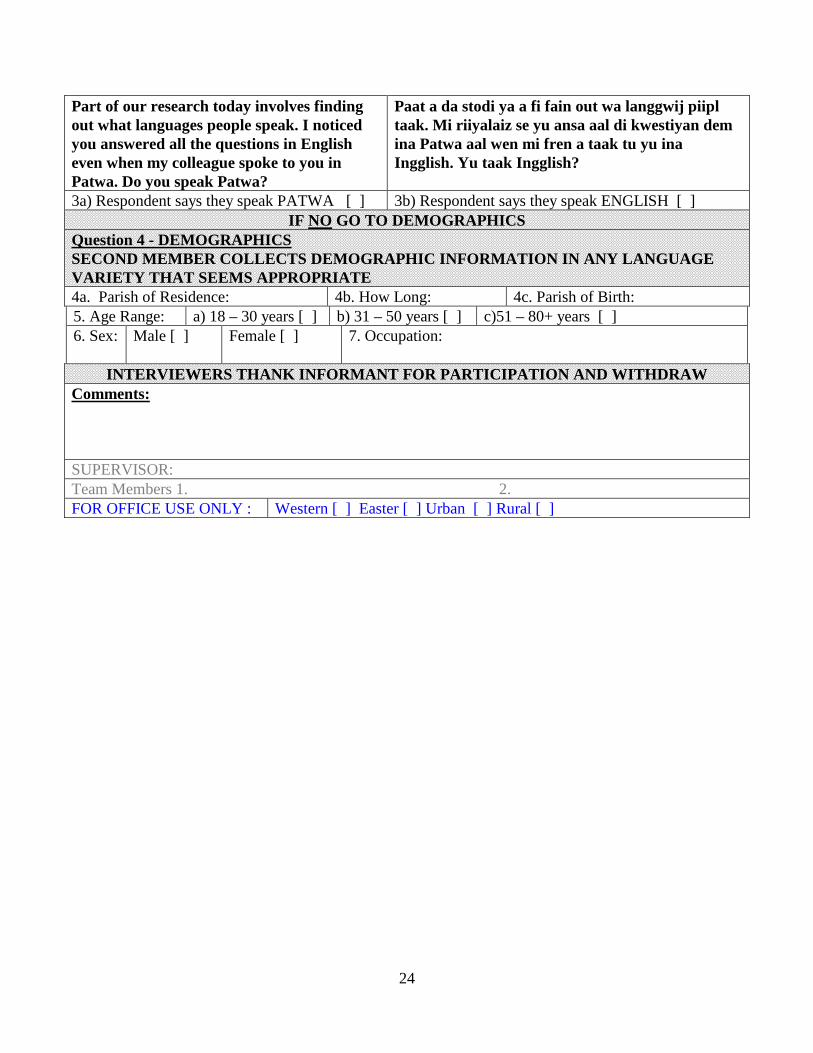
24

Part of our research today involves finding out what languages people speak. I noticed you answered all the questions in English even when my colleague spoke to you in Patwa. Do you speak Patwa?

Paat a da stodi ya a fi fain out wa langgwij piipl taak. Mi riiyalaiz se yu ansa aal di kwestiyan dem ina Patwa aal wen mi fren a taak tu yu ina Ingglish. Yu taak Ingglish?

3a) Respondent says they speak PATWA [ ] 3b) Respondent says they speak ENGLISH [ ] IF NO GO TO DEMOGRAPHICS

Question 4 - DEMOGRAPHICS SECOND MEMBER COLLECTS DEMOGRAPHIC INFORMATION IN ANY LANGUAGE VARIETY THAT SEEMS APPROPRIATE 4a. Parish of Residence: 4b. How Long: 4c. Parish of Birth: 5. Age Range: a) 18 – 30 years [ ] b) 31 – 50 years [ ] c)51 – 80+ years [ ] 6. Sex:

Male [ ] Female [ ] 7. Occupation:

INTERVIEWERS THANK INFORMANT FOR PARTICIPATION AND WITHDRAW Comments: SUPERVISOR: Team Members 1. 2. FOR OFFICE USE ONLY : Western [ ] Easter [ ] Urban [ ] Rural [ ]

25

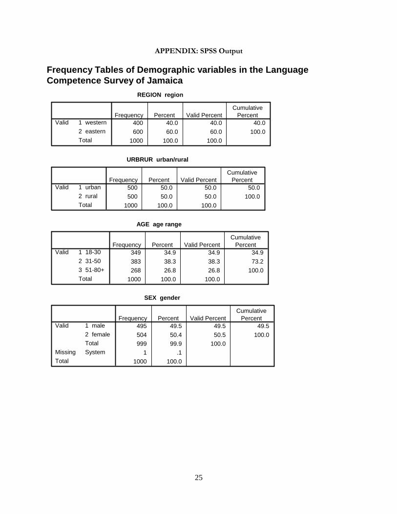
APPENDIX: SPSS Output

Frequency Tables of Demographic variables in the Language Competence Survey of Jamaica

REGION region

400 40.0 40.0 40.0

600 60.0 60.0 100.0

1000 100.0 100.0

1 western

2 eastern

Total

ValidFrequency Percent Valid Percent

CumulativePercent

URBRUR urban/rural

500 50.0 50.0 50.0

500 50.0 50.0 100.0

1000 100.0 100.0

1 urban

2 rural

Total


CumulativePercent

AGE age range

349 34.9 34.9 34.9

383 38.3 38.3 73.2

268 26.8 26.8 100.0

1000 100.0 100.0

1 18-30

2 31-50

3 51-80+

Total


CumulativePercent

SEX gender

495 49.5 49.5 49.5

504 50.4 50.5 100.0

999 99.9 100.0

1 .1

1000 100.0

1 male

2 female

Total

Valid

SystemMissing

Total

Frequency Percent Valid PercentCumulative

Percent

26

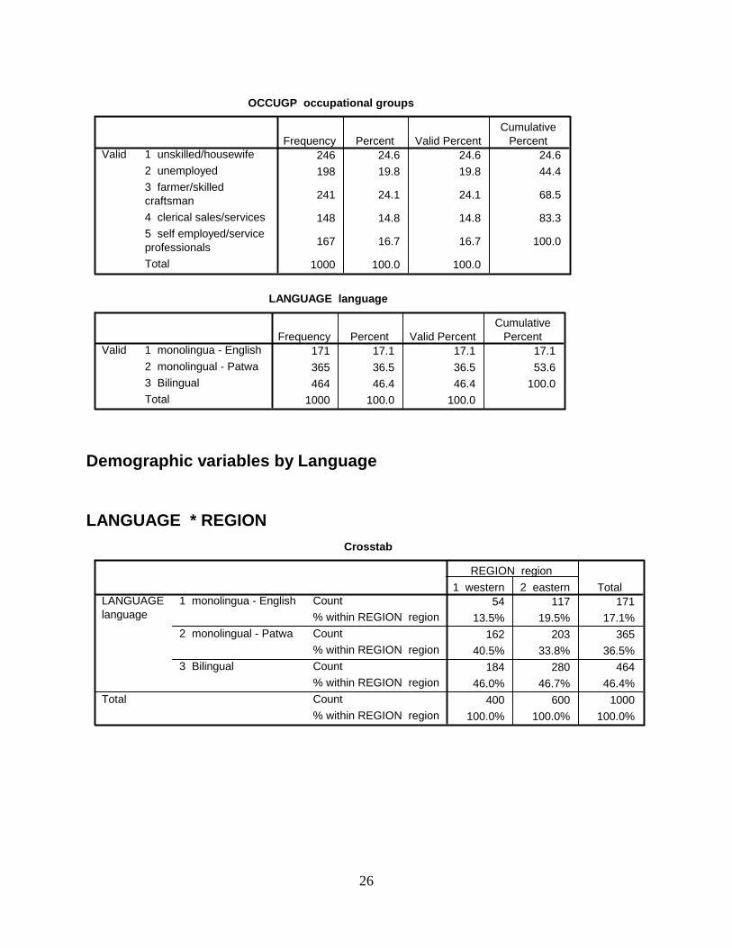
OCCUGP occupational groups

246 24.6 24.6 24.6

198 19.8 19.8 44.4

241 24.1 24.1 68.5

148 14.8 14.8 83.3

167 16.7 16.7 100.0

1000 100.0 100.0

1 unskilled/housewife

2 unemployed

3 farmer/skilledcraftsman

4 clerical sales/services

5 self employed/serviceprofessionals

Total


CumulativePercent

LANGUAGE language

171 17.1 17.1 17.1

365 36.5 36.5 53.6

464 46.4 46.4 100.0

1000 100.0 100.0

1 monolingua - English

2 monolingual - Patwa

3 Bilingual

Total


CumulativePercent

Demographic variables by Language LANGUAGE * REGION

Crosstab

54 117 171

13.5% 19.5% 17.1%

162 203 365

40.5% 33.8% 36.5%

184 280 464

46.0% 46.7% 46.4%

400 600 1000

100.0% 100.0% 100.0%

Count

% within REGION region

Count


Count


Count




3 Bilingual

LANGUAGE language

Total

1 western 2 eastern

REGION region

Total

27

Chi-Square Tests

7.998a 2 .018

8.117 2 .017

1.242 1 .265

1000

Pearson Chi-Square

Likelihood Ratio

Linear-by-LinearAssociation

N of Valid Cases

Value dfAsymp. Sig.

(2-sided)

0 cells (.0%) have expected count less than 5. Theminimum expected count is 68.40.

a.

Symmetric Measures

.089 .018

1000

Contingency CoefficientNominal by Nominal

N of Valid Cases

Value Approx. Sig.

Not assuming the null hypothesis.a.

Using the asymptotic standard error assuming the null hypothesis.b.

LANGUAGE * URBRUR urban/rural Crosstab

103 68 171

20.6% 13.6% 17.1%

163 202 365

32.6% 40.4% 36.5%

234 230 464

46.8% 46.0% 46.4%

500 500 1000

100.0% 100.0% 100.0%

Count

% within URBRURurban/rural

Count


Count


Count




3 Bilingual

LANGUAGE language

Total

1 urban 2 rural

URBRUR urban/rural

Total

28

Chi-Square Tests

11.365a 2 .003

11.424 2 .003

1.748 1 .186

1000

Pearson Chi-Square

Likelihood Ratio


N of Valid Cases

Value dfAsymp. Sig.

(2-sided)


a.

Symmetric Measures

.106 .003

1000


N of Valid Cases

Value Approx. Sig.



LANGUAGE * AGE range

Crosstab

69 60 42 171

19.8% 15.7% 15.7% 17.1%

115 142 108 365

33.0% 37.1% 40.3% 36.5%

165 181 118 464

47.3% 47.3% 44.0% 46.4%

349 383 268 1000

100.0% 100.0% 100.0% 100.0%

Count

% within AGE age range

Count


Count


Count




3 Bilingual

LANGUAGE language

Total

1 18-30 2 31-50 3 51-80+

AGE age range

Total

Chi-Square Tests

4.978a 4 .290

4.941 4 .293

.042 1 .839

1000

Pearson Chi-Square

Likelihood Ratio


N of Valid Cases

Value dfAsymp. Sig.

(2-sided)


a.

29

Symmetric Measures

.070 .290

1000


N of Valid Cases

Value Approx. Sig.



LANGUAGE * SEX gender Crosstab

86 85 171

17.4% 16.9% 17.1%

181 183 364

36.6% 36.3% 36.4%

228 236 464

46.1% 46.8% 46.4%

495 504 999

100.0% 100.0% 100.0%

Count

% within SEX gender

Count

% within SEX gender

Count

% within SEX gender

Count

% within SEX gender



3 Bilingual

LANGUAGE language

Total

1 male 2 female

SEX gender

Total

Chi-Square Tests

.074a 2 .964

.074 2 .964

.074 1 .786

999

Pearson Chi-Square

Likelihood Ratio


N of Valid Cases

Value dfAsymp. Sig.

(2-sided)


a.

Symmetric Measures

.009 .964

999


N of Valid Cases

Value Approx. Sig.



30

LANGUAGE * OCCUGP occupational groups Crosstab

21 45 28 25 52 171

8.5% 22.7% 11.6% 16.9% 31.1% 17.1%

127 66 100 36 36 365

51.6% 33.3% 41.5% 24.3% 21.6% 36.5%

98 87 113 87 79 464

39.8% 43.9% 46.9% 58.8% 47.3% 46.4%

246 198 241 148 167 1000

100.0% 100.0% 100.0% 100.0% 100.0% 100.0%

Count

% within OCCUGP occupational groups

Count


Count


Count




3 Bilingual

LANGUAGE language

Total


2 unemployed

3 farmer/skilled

craftsman

4 clericalsales/ser

vices

5 selfemployed/ser

viceprofessionals


Total

Chi-Square Tests

79.013a 8 .000

78.307 8 .000

.338 1 .561

1000

Pearson Chi-Square

Likelihood Ratio


N of Valid Cases

Value dfAsymp. Sig.

(2-sided)


a.

Symmetric Measures

.271 .000

1000


N of Valid Cases

Value Approx. Sig.



31

Controlling for Sex of Interviewers LANGUAGE * REGION * Q11 Sex of Interviewers

Crosstab

11 43 54

8.5% 20.7% 16.0%

50 74 124

38.8% 35.6% 36.8%

68 91 159

52.7% 43.8% 47.2%

129 208 337

100.0% 100.0% 100.0%

43 74 117

15.9% 18.9% 17.6%

112 129 241

41.3% 32.9% 36.3%

116 189 305

42.8% 48.2% 46.0%

271 392 663

100.0% 100.0% 100.0%

Count


Count


Count


Count


Count


Count


Count


Count




3 Bilingual

LANGUAGE language

Total



3 Bilingual

LANGUAGE language

Total

Q11 Sex of Interviewers1 Male & Female

2 Female & Female

1 western 2 eastern

REGION region

Total

Chi-Square Tests

8.905a 2 .012

9.587 2 .008

6.612 1 .010

337

4.967b 2 .083

4.948 2 .084

.166 1 .684

663

Pearson Chi-Square

Likelihood Ratio


N of Valid Cases

Pearson Chi-Square

Likelihood Ratio


N of Valid Cases


2 Female & Female

Value dfAsymp. Sig.

(2-sided)

0 cells (.0%) have expected count less than 5. The minimum expected count is20.67.

a.


b.

32

Symmetric Measures

.160 .012

337

.086 .083

663


N of Valid Cases


N of Valid Cases


2 Female & Female

Value Approx. Sig.



LANGUAGE * URBRUR urban/rural * Q11 Sex of Interviewers

Crosstab

31 23 54

20.5% 12.4% 16.0%

55 69 124

36.4% 37.1% 36.8%

65 94 159

43.0% 50.5% 47.2%

151 186 337

100.0% 100.0% 100.0%

72 45 117

20.6% 14.3% 17.6%

108 133 241

30.9% 42.4% 36.3%

169 136 305

48.4% 43.3% 46.0%

349 314 663

100.0% 100.0% 100.0%

Count


Count


Count


Count


Count


Count


Count


Count




3 Bilingual

LANGUAGE language

Total



3 Bilingual

LANGUAGE language

Total


2 Female & Female

1 urban 2 rural

URBRUR urban/rural

Total

33

Chi-Square Tests

4.468a 2 .107

4.451 2 .108

3.807 1 .051

337

10.576b 2 .005

10.614 2 .005

.042 1 .838

663

Pearson Chi-Square

Likelihood Ratio


N of Valid Cases

Pearson Chi-Square

Likelihood Ratio


N of Valid Cases


2 Female & Female

Value dfAsymp. Sig.

(2-sided)


a.


b.

Symmetric Measures

.114 .107

337

.125 .005

663


N of Valid Cases


N of Valid Cases


2 Female & Female

Value Approx. Sig.



LANGUAGE * AGE range * Q11 Sex of Interviewers Crosstab

22 22 10 54

18.6% 16.8% 11.4% 16.0%

38 51 35 124

32.2% 38.9% 39.8% 36.8%

58 58 43 159

49.2% 44.3% 48.9% 47.2%

118 131 88 337

100.0% 100.0% 100.0% 100.0%

47 38 32 117

20.3% 15.1% 17.8% 17.6%

77 91 73 241

33.3% 36.1% 40.6% 36.3%

107 123 75 305

46.3% 48.8% 41.7% 46.0%

231 252 180 663

100.0% 100.0% 100.0% 100.0%

Count


Count


Count


Count


Count


Count


Count


Count




3 Bilingual

LANGUAGE language

Total



3 Bilingual

LANGUAGE language

Total


2 Female & Female

1 18-30 2 31-50 3 51-80+

AGE age range

Total

34

Chi-Square Tests

3.182a 4 .528

3.316 4 .506

.369 1 .543

337

4.527b 4 .339

4.532 4 .339

.028 1 .866

663

Pearson Chi-Square

Likelihood Ratio


N of Valid Cases

Pearson Chi-Square

Likelihood Ratio


N of Valid Cases


2 Female & Female

Value dfAsymp. Sig.

(2-sided)


a.


b.

Symmetric Measures

.097 .528

337

.082 .339

663


N of Valid Cases


N of Valid Cases


2 Female & Female

Value Approx. Sig.



LANGUAGE * SEX gender * Q11 Sex of Interviewers Crosstab

25 29 54

16.8% 15.4% 16.0%

56 68 124

37.6% 36.2% 36.8%

68 91 159

45.6% 48.4% 47.2%

149 188 337

100.0% 100.0% 100.0%

61 56 117

17.6% 17.7% 17.7%

125 115 240

36.1% 36.4% 36.3%

160 145 305

46.2% 45.9% 46.1%

346 316 662

100.0% 100.0% 100.0%

Count

% within SEX gender

Count

% within SEX gender

Count

% within SEX gender

Count

% within SEX gender

Count

% within SEX gender

Count

% within SEX gender

Count

% within SEX gender

Count

% within SEX gender



3 Bilingual

LANGUAGE language

Total



3 Bilingual

LANGUAGE language

Total


2 Female & Female

1 male 2 female

SEX gender

Total

35

Chi-Square Tests

.275a 2 .872

.275 2 .872

.263 1 .608

337

.009b 2 .996

.009 2 .996

.006 1 .939

662

Pearson Chi-Square

Likelihood Ratio


N of Valid Cases

Pearson Chi-Square

Likelihood Ratio


N of Valid Cases


2 Female & Female

Value dfAsymp. Sig.

(2-sided)


a.


b.

Symmetric Measures

.029 .872

337

.004 .996

662


N of Valid Cases


N of Valid Cases


2 Female & Female

Value Approx. Sig.



36

LANGUAGE * OCCUGP occupational groups * Q11 Sex of Interviewers Crosstab

6 18 9 7 14 54

7.1% 27.3% 11.7% 14.6% 22.6% 16.0%

50 17 31 13 13 124

59.5% 25.8% 40.3% 27.1% 21.0% 36.8%

28 31 37 28 35 159

33.3% 47.0% 48.1% 58.3% 56.5% 47.2%

84 66 77 48 62 337

100.0% 100.0% 100.0% 100.0% 100.0% 100.0%

15 27 19 18 38 117

9.3% 20.5% 11.6% 18.0% 36.2% 17.6%

77 49 69 23 23 241

47.5% 37.1% 42.1% 23.0% 21.9% 36.3%

70 56 76 59 44 305

43.2% 42.4% 46.3% 59.0% 41.9% 46.0%

162 132 164 100 105 663

100.0% 100.0% 100.0% 100.0% 100.0% 100.0%

Count


Count


Count


Count


Count


Count


Count


Count




3 Bilingual

LANGUAGE language

Total



3 Bilingual

LANGUAGE language

Total


2 Female & Female


2 unemployed

3 farmer/skilled

craftsman

4 clericalsales/ser

vices

5 selfemployed/ser

viceprofessionals


Total

Chi-Square Tests

37.478a 8 .000

37.080 8 .000

1.740 1 .187

337

53.632b 8 .000

51.540 8 .000

2.817 1 .093

663

Pearson Chi-Square

Likelihood Ratio


N of Valid Cases

Pearson Chi-Square

Likelihood Ratio


N of Valid Cases


2 Female & Female

Value dfAsymp. Sig.

(2-sided)


a.


b.

37

Symmetric Measures

.316 .000

337

.274 .000

663


N of Valid Cases


N of Valid Cases


2 Female & Female

Value Approx. Sig.



Controlling for Language used to Initiate Interview LANGUAGE * URBRUR urban/rural * Q12 Starters

Crosstab

54 29 83

21.6% 13.3% 17.7%

74 96 170

29.6% 44.0% 36.3%

122 93 215

48.8% 42.7% 45.9%

250 218 468

100.0% 100.0% 100.0%

49 39 88

19.6% 13.8% 16.5%

89 106 195

35.6% 37.6% 36.7%

112 137 249

44.8% 48.6% 46.8%

250 282 532

100.0% 100.0% 100.0%

Count


Count


Count


Count


Count


Count


Count


Count




3 Bilingual

LANGUAGE language

Total



3 Bilingual

LANGUAGE language

Total

Q12 Starters1 English starter

2 Patwa Starter

1 urban 2 rural

URBRUR urban/rural

Total

38

Chi-Square Tests

12.158a 2 .002

12.237 2 .002

.097 1 .755

468

3.215b 2 .200

3.211 2 .201

2.227 1 .136

532

Pearson Chi-Square

Likelihood Ratio


N of Valid Cases

Pearson Chi-Square

Likelihood Ratio


N of Valid Cases


2 Patwa Starter

Value dfAsymp. Sig.

(2-sided)

0 cells (.0%) have expected count less than 5. The minimum expected countis 38.66.

a.


b.

Symmetric Measures

.159 .002

468

.078 .200

532


N of Valid Cases


N of Valid Cases


2 Patwa Starter

Value Approx. Sig.



LANGUAGE * AGE range * Q12 Starters Crosstab

27 34 22 83

15.5% 17.8% 21.4% 17.7%

60 68 42 170

34.5% 35.6% 40.8% 36.3%

87 89 39 215

50.0% 46.6% 37.9% 45.9%

174 191 103 468

100.0% 100.0% 100.0% 100.0%

42 26 20 88

24.0% 13.5% 12.1% 16.5%

55 74 66 195

31.4% 38.5% 40.0% 36.7%

78 92 79 249

44.6% 47.9% 47.9% 46.8%

175 192 165 532

100.0% 100.0% 100.0% 100.0%

Count


Count


Count


Count


Count


Count


Count


Count




3 Bilingual

LANGUAGE language

Total



3 Bilingual

LANGUAGE language

Total


2 Patwa Starter

1 18-30 2 31-50 3 51-80+

AGE age range

Total

39

Chi-Square Tests

4.102a 4 .392

4.134 4 .388

3.551 1 .060

468

11.151b 4 .025

10.746 4 .030

3.672 1 .055

532

Pearson Chi-Square

Likelihood Ratio


N of Valid Cases

Pearson Chi-Square

Likelihood Ratio


N of Valid Cases


2 Patwa Starter

Value dfAsymp. Sig.

(2-sided)


a.


b.

Symmetric Measures

.093 .392

468

.143 .025

532


N of Valid Cases


N of Valid Cases


2 Patwa Starter

Value Approx. Sig.



40

LANGUAGE * SEX gender * Q12 Starters Crosstab

39 44 83

17.6% 17.8% 17.7%

78 92 170

35.3% 37.2% 36.3%

104 111 215

47.1% 44.9% 45.9%

221 247 468

100.0% 100.0% 100.0%

47 41 88

17.2% 16.0% 16.6%

103 91 194

37.6% 35.4% 36.5%

124 125 249

45.3% 48.6% 46.9%

274 257 531

100.0% 100.0% 100.0%

Count

% within SEX gender

Count

% within SEX gender

Count

% within SEX gender

Count

% within SEX gender

Count

% within SEX gender

Count

% within SEX gender

Count

% within SEX gender

Count

% within SEX gender



3 Bilingual

LANGUAGE language

Total



3 Bilingual

LANGUAGE language

Total


2 Patwa Starter

1 male 2 female

SEX gender

Total

Chi-Square Tests

.238a 2 .888

.238 2 .888

.109 1 .741

468

.612b 2 .736

.612 2 .736

.512 1 .474

531

Pearson Chi-Square

Likelihood Ratio


N of Valid Cases

Pearson Chi-Square

Likelihood Ratio


N of Valid Cases


2 Patwa Starter

Value dfAsymp. Sig.

(2-sided)


a.


b.

41

Symmetric Measures

.023 .888

468

.034 .736

531


N of Valid Cases


N of Valid Cases


2 Patwa Starter

Value Approx. Sig.



LANGUAGE * OCCUGP occupational groups * Q12 Starters

Crosstab

10 20 16 13 24 83

9.8% 21.1% 14.3% 18.3% 27.3% 17.7%

52 32 45 18 23 170

51.0% 33.7% 40.2% 25.4% 26.1% 36.3%

40 43 51 40 41 215

39.2% 45.3% 45.5% 56.3% 46.6% 45.9%

102 95 112 71 88 468

100.0% 100.0% 100.0% 100.0% 100.0% 100.0%

11 25 12 12 28 88

7.6% 24.3% 9.3% 15.6% 35.4% 16.5%

75 34 55 18 13 195

52.1% 33.0% 42.6% 23.4% 16.5% 36.7%

58 44 62 47 38 249

40.3% 42.7% 48.1% 61.0% 48.1% 46.8%

144 103 129 77 79 532

100.0% 100.0% 100.0% 100.0% 100.0% 100.0%

Count


Count


Count


Count


Count


Count


Count


Count




3 Bilingual

LANGUAGE language

Total



3 Bilingual

LANGUAGE language

Total


2 Patwa Starter


2 unemployed

3 farmer/skilled

craftsman

4 clericalsales/ser

vices

5 selfemployed/ser

viceprofessionals


Total

42

Chi-Square Tests

23.722a 8 .003

23.611 8 .003

.105 1 .746

468

60.378b 8 .000

59.661 8 .000

.209 1 .648

532

Pearson Chi-Square

Likelihood Ratio


N of Valid Cases

Pearson Chi-Square

Likelihood Ratio


N of Valid Cases


2 Patwa Starter

Value dfAsymp. Sig.

(2-sided)


a.


b.

Symmetric Measures

.220 .003

468

.319 .000

532


N of Valid Cases


N of Valid Cases


2 Patwa Starter

Value Approx. Sig.



Documents

The Language Competence Survey of Jamaica Language Competence Survey of Jamaica...language. This year’s study: the Language Competence Survey of Jamaica (LCS) however concentrated