The Laplace driven moving average – a non-Gaussian stationary

The Laplace driven moving average– a non-Gaussian stationary process

Sofia Aberg1, Krzysztof Podgorski2, Igor Rychlik1

1Mathematical Sciences, Mathematical Statistics, Chalmers2Centre for Mathematical Sciences, Mathematical Statistics, Lund

Smogen, August 2008

Sofia Aberg Laplace driven MA

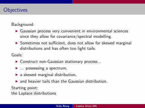
Objectives

Background:

I Gaussian process very convenient in environmental sciencessince they allow for covariance/spectral modelling.

I Sometimes not sufficient, does not allow for skewed marginaldistributions and has often too light tails.

Goals:

I Construct non-Gaussian stationary process...

I ... possessing a spectrum,

I a skewed marginal distribution,

I and heavier tails than the Gaussian distribution.

Starting point:the Laplace distributions


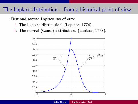
The Laplace distribution – from a historical point of view

First and second Laplace law of error.

I. The Laplace distribution. (Laplace, 1774).

II. The normal (Gauss) distribution. (Laplace, 1778).

−5 0 50

0.05

0.1

0.15

0.2

0.25

0.3

0.35

0.4

0.45

0.5

1

2e−|x| 1√

2πe−x2/2


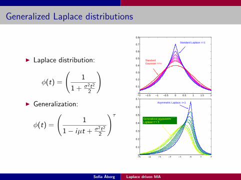
Generalized Laplace distributions

I Laplace distribution:

φ(t) =

(1

1 + σ2t2

2

)

I Generalization:

φ(t) =

(1

1− iµt + σ2t2

2

)τ

−2 −1.5 −1 −0.5 0 0.5 1 1.5 20

0.1

0.2

0.3

0.4

0.5

0.6

0.7

0.8

Standard Laplace: τ=1

StandardGaussian: τ=∞

−5 −4 −3 −2 −1 0 1 20

0.1

0.2

0.3

0.4

0.5

0.6

0.7Asymmetric Laplace: τ=1

Generalized asymmetricLaplace: τ = 3


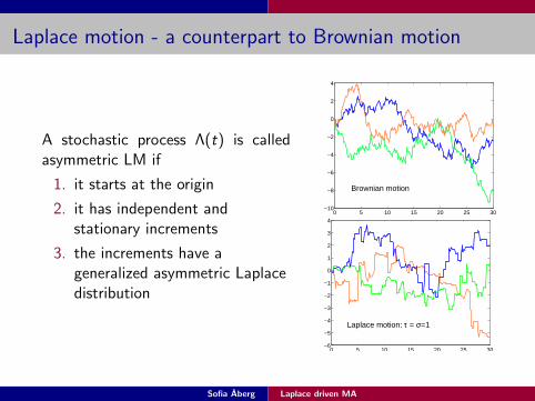
Laplace motion - a counterpart to Brownian motion

A stochastic process Λ(t) is calledasymmetric LM if

1. it starts at the origin

2. it has independent andstationary increments

3. the increments have ageneralized asymmetric Laplacedistribution

0 5 10 15 20 25 30−10

−8

−6

−4

−2

0

2

4

Brownian motion

0 5 10 15 20 25 30−6

−5

−4

−3

−2

−1

0

1

2

3

4

Laplace motion: τ = σ=1


The Laplace driven moving average

Using the Laplace motion Λ(x) one can define a Laplace drivenmoving average by

X (t) =

∫ ∞

−∞f (t − x)dΛ(x).

The function f is called a kernel and should satisfy∫f 2(x) dx < ∞. A similar definition is possible in higher

dimensions.


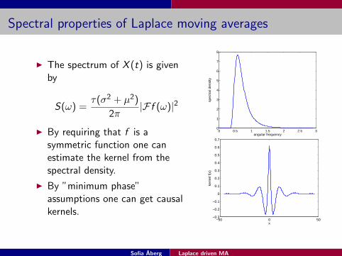
Spectral properties of Laplace moving averages

I The spectrum of X (t) is givenby

S(ω) =τ(σ2 + µ2)

2π|F f (ω)|2

I By requiring that f is asymmetric function one canestimate the kernel from thespectral density.

I By ”minimum phase”assumptions one can get causalkernels.

0 0.5 1 1.5 2 2.5 30

1

2

3

4

5

6

7

8

spec

tral

den

sity

angular frequency

−50 0 50−0.3

−0.2

−0.1

0

0.1

0.2

0.3

0.4

0.5

0.6

0.7

x

kern

el f(

x)


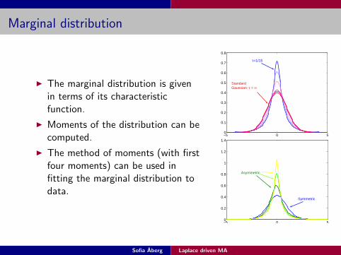
Marginal distribution

I The marginal distribution is givenin terms of its characteristicfunction.

I Moments of the distribution can becomputed.

I The method of moments (with firstfour moments) can be used infitting the marginal distribution todata.

−5 0 50

0.1

0.2

0.3

0.4

0.5

0.6

0.7

0.8

τ=1/15

StandardGaussian: τ = ∞

−5 0 50

0.2

0.4

0.6

0.8

1

1.2

1.4

Symmetric

Asymmetric


Simulation

The LMA can be seen as a convolution of Laplace noise with akernel f . Discrete version:

∫f (t − x)dΛ(x) ≈

∑f (t − xi )∆Λ(xi )

Time domain simulation:

I simulate iid Laplace noise

I convolve the noise with the kernel

Frequency domain simulation:

I simulate iid Laplace noise

I Fourier transform the noise and the kernel f using FFT

I Take product of the Fourier transforms

I Take inverse Fourier transform of the product


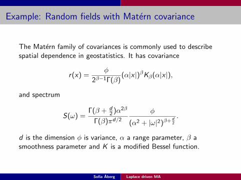
Example: Random fields with Matern covariance

The Matern family of covariances is commonly used to describespatial dependence in geostatistics. It has covariance

r(x) =φ

2β−1Γ(β)(α|x |)βKβ(α|x |),

and spectrum

S(ω) =Γ(β + d

2 )α2β

Γ(β)πd/2

φ

(α2 + |ω|2)β+ d2

.

d is the dimension φ is variance, α a range parameter, β asmoothness parameter and K is a modified Bessel function.


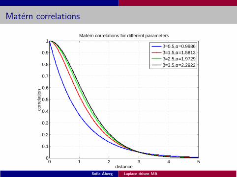
Matern correlations

0 1 2 3 4 50

0.1

0.2

0.3

0.4

0.5

0.6

0.7

0.8

0.9

1

distance

corr

elat

ion

Matérn correlations for different parameters

β=0.5,α=0.9986β=1.5,α=1.5813β=2.5,α=1.9729β=3.5,α=2.2922


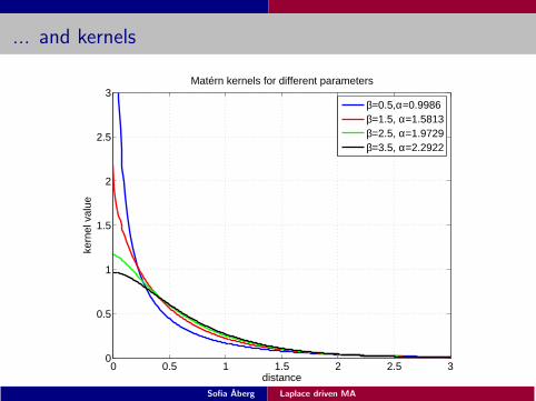
... and kernels

0 0.5 1 1.5 2 2.5 30

0.5

1

1.5

2

2.5

3

distance

kern

el v

alueMatérn kernels for different parameters

β=0.5,α=0.9986β=1.5, α=1.5813β=2.5, α=1.9729β=3.5, α=2.2922


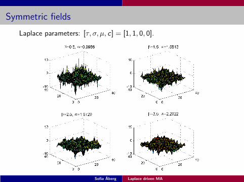
Symmetric fields

Laplace parameters: [τ, σ, µ, c] = [1, 1, 0, 0].


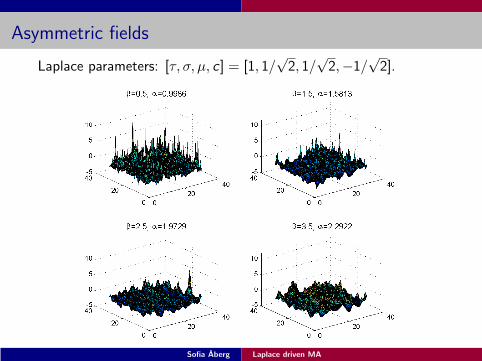
Asymmetric fields

Laplace parameters: [τ, σ, µ, c] = [1, 1/√

2, 1/√

2,−1/√

2].


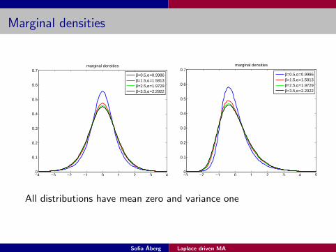
Marginal densities

−4 −3 −2 −1 0 1 2 3 40

0.1

0.2

0.3

0.4

0.5

0.6

0.7marginal densities

β=0.5,α=0.9986β=1.5,α=1.5813β=2.5,α=1.9729β=3.5,α=2.2922

−3 −2 −1 0 1 2 3 4 50

0.1

0.2

0.3

0.4

0.5

0.6

0.7marginal densities

β=0.5,α=0.9986β=1.5,α=1.5813β=2.5,α=1.9729β=3.5,α=2.2922

All distributions have mean zero and variance one


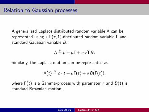
Relation to Gaussian processes

A generalized Laplace distributed random variable Λ can berepresented using a Γ(τ, 1)-distributed random variable Γ andstandard Gaussian variable B:

ΛD= c + µΓ + σ

√ΓB.

Similarly, the Laplace motion can be represented as

Λ(t)D= c · t + µΓ(t) + σB(Γ(t)),

where Γ(t) is a Gamma-process with parameter τ and B(t) isstandard Brownian motion.


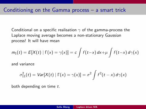
Conditioning on the Gamma process – a smart trick

Conditional on a specific realisation γ of the gamma-process theLaplace moving average becomes a non-stationary Gaussianprocess! It will have mean

m1(t) = E [X (t) | Γ(x) = γ(x)] = c

∫f (t−x) dx+µ

∫f (t−x) dγ(x)

and variance

σ211(t) = Var [X (t) | Γ(x) = γ(x)] = σ2

∫f 2(t − x) dγ(x)

both depending on time t.


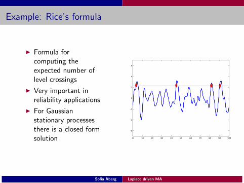
Example: Rice’s formula

I Formula forcomputing theexpected number oflevel crossings

I Very important inreliability applications

I For Gaussianstationary processesthere is a closed formsolution 0 10 20 30 40 50 60 70 80 90 100

−6

−4

−2

0

2

4

6


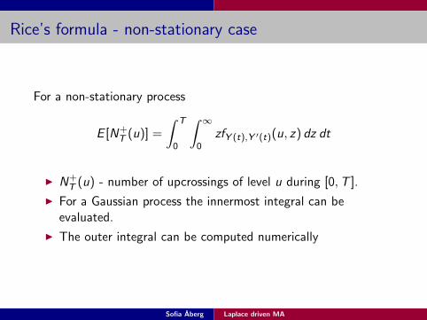
Rice’s formula - non-stationary case

For a non-stationary process

E [N+T (u)] =

∫ T

0

∫ ∞

0zfY (t),Y ′(t)(u, z) dz dt

I N+T (u) - number of upcrossings of level u during [0, T ].

I For a Gaussian process the innermost integral can beevaluated.

I The outer integral can be computed numerically


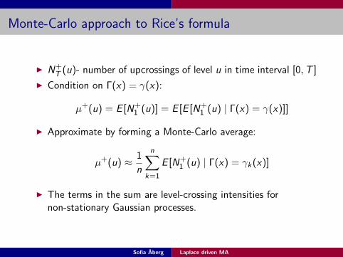
Monte-Carlo approach to Rice’s formula

I N+T (u)- number of upcrossings of level u in time interval [0,T ]

I Condition on Γ(x) = γ(x):

µ+(u) = E [N+1 (u)] = E [E [N+

1 (u) | Γ(x) = γ(x)]]

I Approximate by forming a Monte-Carlo average:

µ+(u) ≈ 1

n

n∑

k=1

E [N+1 (u) | Γ(x) = γk(x)]

I The terms in the sum are level-crossing intensities fornon-stationary Gaussian processes.


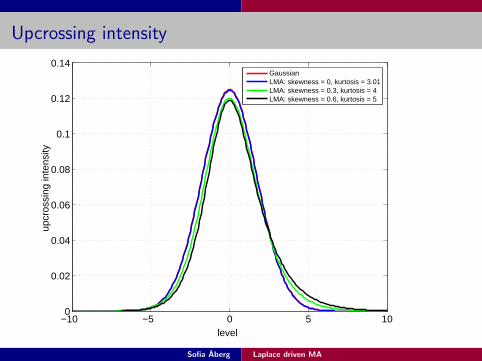
Upcrossing intensity

−10 −5 0 5 100

0.02

0.04

0.06

0.08

0.1

0.12

0.14

level

upcr

ossi

ng in

tens

ity

GaussianLMA: skewness = 0, kurtosis = 3.01LMA: skewness = 0.3, kurtosis = 4LMA: skewness = 0.6, kurtosis = 5


Summary

I The Laplace driven moving average can be used to modelsecond order stationary loads with skewed marginaldistribution.

I The model can be fitted to data using a moment matchingapproach.

I Simulation can either be done in time or in frequency domain.

I Conditional on a realisation of a gamma-process the LMAbecomes a non-stationary Gaussian process.

I Rice’s formula can be evaluated by a Monte-Carlo method.


Documents

The Laplace driven moving average – a non-Gaussian stationary