1

The Laplace Transform

Prof. Siripong Potisuk

Pierre Simon De Laplace

French Astronomer and Mathematician

1749 - 1827

2

Laplace Transform

An extension of the CT Fourier transform to

allow analysis of broader class of CT signals

and systems

Handle an important class of unstable

systems whose signals are not absolutely

integrable, i.e.,

3

Conditions for CTFT Existence

Applicable for aperiodic signal of finite and

infinite duration which satisfies:

dttx 2|)(| : Energy Finite)b(

Conditions set' Dirichl(a)

Bilateral Laplace Transform

Satisfy the condition of absolute integrability

by multiplying x(t) by a convergence factor

e-t for some value of

Combine the exponentials and let s = +j

})({})({)( ttjt etxCTFTtdeetxjX

4

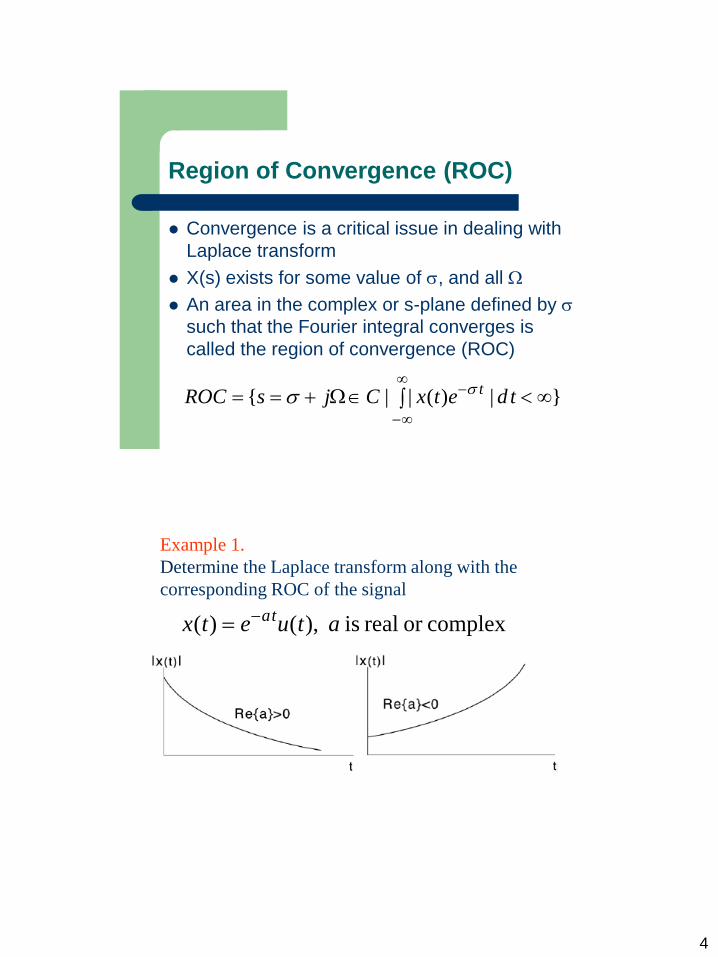
Region of Convergence (ROC)

Convergence is a critical issue in dealing with

Laplace transform

X(s) exists for some value of , and all

An area in the complex or s-plane defined by

such that the Fourier integral converges is

called the region of convergence (ROC)

}|)(||{

tdetxCjsROC t

Example 1.

Determine the Laplace transform along with the

corresponding ROC of the signal

complexor real is ),()( atuetx ta

5

Example 2.

Determine the Laplace transform along with the

corresponding ROC of the signal

complexor real is ),()( atuetx ta

6

Example 3.

Determine the Laplace transform along with the

corresponding ROC of the signals

tCetxa t ,)( )(

tetybtj,)( )( 0

Rational Laplace Transform

For most practical signals, the Laplace transform can be

expressed as a ratio of two polynomials

.polynomialr denominato theof

roots thei.e.,, of theare ,,, and

polynomialnumerator theof

roots thei.e.,, of theare ,,, where

)())((

)())((

)(

)()(

21

21

210

210

X(s)polesppp

X(s)zeroeszzz

pspspsa

zszszsb

sD

sNsX

N

M

N

M

7

Rational Laplace Transform

NNN

MMM

N

M

asas

bsbsb

pspsps

zszszsb

sD

sNsX

11

110

21

210

)())((

)())((

)(

)()(

It is customary to normalize the denominator polynomial

to make its leading coefficients one, i.e.,

Also, X(s) is a proper rational transform if

poles. of # zeroes of # i.e., , NM

The complex s-plane

s + j

(Re{s})

(Im{s})

8

The pole-zero plot of a rational Laplace transform in the s-plane.

Laplace Transform Properties

Parallel many of the CTFT properties, except

for the need to specify ROC

Linearity:

Time-shifting

9

Example 4.

Determine the Laplace transform along with the

corresponding ROC of the signal

2( ) 3 ( ) 2 ( )t tx t e u t e u t

Properties of the ROC

10

11

12

7) If X(s) is rational, its ROC is bounded by poles or extends

to infinity. Also, no poles of X(s) are contained in the ROC.

(a) x(t) right-sided ROC to the right of rightmost pole

(b) x(t) left-sided ROC to the left of leftmost pole

(c) x(t) two-sided ROC a strip between two poles

8) ROC of x(t) contains j-axis CTFT of x(t) exists

13

Inverse Laplace Transform

Transform back from the s-domain to the time

domain

Generally, computed by

For rational Laplace transform, expand in terms

of partial fractions and use table of transform

pairs and properties

From the previous example, the time-domain signal, x(t),

resulting from the inversion process for each ROC is

14

Example 5.

Determine the number of all possible signals that have

similar Laplace transform below but different ROCs.

)1)(3)(2(

1)(

2

ssss

ssX

15

Convolution Property

L

input of transformLaplace

output of transformLaplace

)(

)()(

sX

sYsH

Eigenfunctions of LTI Systems

An eigenfunction of a system is an input signal that,

when applied to a system, results in the output being

the scaled version of itself.

The scaling factor is known as the system’s eigenvalue.

Complex exponentials are eigenfunctions of LTI

systems, i.e., the response of an LTI system to a

complex exponential input is the same complex

exponential with only a change in amplitude.

16

H(s) = L{h(t)} = Laplace transform of impulse response

H(s) is called the system function or transfer function

Checking Causality of LTI Systems

A causal LTI system has a causal impulse

response (i.e., h(t) < 0 for t < 0)

ROC of transfer function for a causal system is a

RHP, but the converse is not true

However, a system with rational transfer function

is causal iff its ROC is the plane to the right of

the rightmost pole

Similar statements can be said about an anti-

causal system

17

Checking Stability of LTI Systems

A BIBO stable LTI system has an absolutely

integrable impulse response (i.e., CTFT of the

impulse response converges)

Consequently, an LTI system is BIBO stable iff

the ROC of its transfer function includes the

entire j-axis

In terms of poles, a causal system with rational

transfer function is BIBO stable iff all of the poles

lie in the LHP (i.e., all poles have negative real

parts)

ROC of transfer function for a causal system is a

RHP, but the converse is not true

However, a system with rational transfer function

is causal iff its ROC is the RHP to the right of the

rightmost pole

Similar statements can be said about an anti-

causal system

The Unilateral Laplace Transform

- The unilateral Laplace transform of a CT signal x(t)

is defined as

tdetxsX st

0

)()(

- Equivalent to the bilateral Laplace transform of x(t)u(t)

- Since x(t)u(t) is always a right-sided signal, ROC of

X(s) always includes the RHP

- Useful for solving LCCDEs with initial conditions