3vtza

TIIE LARGE SCALE STRUCTURE IN TI^IO-DIMENSIONAL VORTICITY

LAYERS AND THE CENIRE-TO-CENTRE POINT-VORTEX APPROXIMATION

by

Bernard A. Delcourt,

Ingénieur Civil Physicien(Université de Liège, Belgium)

'A thesis presenÈed to the Faculty

of Engineering of the University of Adelaide

for the Degree of Doctor of Philosophy

Department of Mechanical Engineering,

University of Adelaide.

ApríL 1980.

TABLE OF CONTENTS

GENERAL INTRODUCTION

Chapter I INTRODUCING THE THEORY OF POINT-VORTICES

I.1 INTRODUCTION

,2 ROTATIONAL FLOW FIELDS OF INCOMPRESSIBLEFLUIDS

.3 INTEGRAL INVARIANTS OF TIIIO-DIMENSIONALVORTICITY DISTRIBUTIONS

T..4 COMPLEX THEORY OF POINT-VORTICES

I.4.I The "or,""pt of the point-vortex

I.4.2 The motion of point-vortices

I.4.3 The isolated cloud of point-vortices

T,4,4 The periodic cloud of point-vortices

I.4.5 Hamiltonian formulation

I.5 ST]MMARY

Chapter II THE CENTRE-TO-CENTRE POINT-VORTEX APPROXIMATION

II.I INTRODUCTION

II.2 THE POINT-VORTEX APPROXIMATION

TT.2.1 OuÈline of the method

TI.2.2 The development and substance ofËhe PVA

II.3 THE CLOUD DISCRETIZATION APPROACH

II.4 THE CENTRE-TO-CENTRE METHOD

I

2

I

I

I

Page number

L4

L7

18

20

2L

25

26

27

35

30

37

II.5

II.6

TT.7

II.8

EFFECTS OF INTEGRATION PROCEDURE, TIME STEPAND CELL SIZE IN THE CTC METHOD

II.5.1 Rankiners vorEex

II.5.2 The PVA of Rankiners vortex

II.5.3 Eulerrs integration method

II.5.4 Huenrs integration method

VISCOUS EFFECTS IN THE CTC METHOD

II.6.1 Viscous decay of a vortícity disk

II.6.2 The evaluation of H(t) ana ot ti(t)

II.6.3 Viscosity estímates

II.6.4 Díscussion of results

THE ROLLING-UP OF A VORTEX SHEET

IT-.7 .1 l.IeswaÈer I s ro11 up problem

II.7.2 The cloud discretizatíon approach

SUMMARY

POINT-VORTEX MODELLING OF TURBULENTMIXING LAYERS

III.3.1 Periodic vorticity layers

III.3.2 The initial flow configurations

III.3.3 Selecting time step and ce1l size

III.3.4 Actonrs míxing layer model

THE INVISCID VORTICITY LAYERS

40

4L

44

46

49

51

53

57

62

64

66

69

74

76

7B

83

Chapter III THE LARGE-SCALE STRUCTURE IN PERIODIC, TI^IO-DIMENSIONAL VORTICITY LAYERS

III. 1-

TTT.2

INTRODUCTION

THE TURBULENT MIXING LAYER IN THELABORATORY

III.3

III.4

80

85

III.5

III. 6

III.4.1 Computed flow patterns

III.4.2 The growth of the layers

III.4.3 Correlation analysis of thevelocity field

THE VISCOUS VORTICITY LAYERS

III.5.1 Viscous and turbular computations

III.5.2 Low Reynolds number layers

SI.JM},ÍARY

87

90

97

103

106

107

109

110

111

TL2

113

115

116

L22

Chapter IV THE POINT-VORTEX APPROXII'ÍATION OF NON CIRCULATIONPRESERVING FLOI,','S

IV.1 INTRODUCTION

TV.z CREATION OF CIRCULATION IN A FLUID IN MOTION

TV.2.1 Vect,or flux across a materialsurface

rv.2 .2 Acceleration, vorticity andexpansion

TV.2.3 Rate of change of circulaËion

TV.2,4 Bjerknes theorem

rv.3 POINT-VORTEX MODELLING OF NON CIRCULATIONPRESERVING MOTIONS

rv.3. 1

TV.3.2

The fundamental approach

ComputaEion of rlo

IV.4 DENSITY EFFECTS ON THE STRUCTURE OFVORTICITY LAYERS

IV.4.1 The temporal problem for two-density layers

IV.4.2 Effect of density ratio on ÈhesÈructure in a sinusoidal vortieitylayer L25

IV.4.3 Froude number effect on t.he structurein a sinusoidal vorticíty layer L28

IV.5 SI]MMARY 130

r

SUMMARY

The large-scale strucÈure whièh emerges spontaneously from random

periodic vorticity layers is studied by a novel discrete vortex element

method.

The validity of the poinE-vortex approximation is examined in terms

of its ability to represenE the integral invariants of two-dimensional

conEinuous vorticity distribuÈions. The method is retained to sËudy the

large-scale moÈions in rotational flows where the exact behaviour of

índividual vortices is largely irrelevant ("cloud discretization" approaeh).

A new, simple and computationally economical point-vortex tracing scheme

is presented. The properties of the rrcentre-to-centreil method, which

preservesnotably the ínvariance of the energy of the vortex system, are

established in reference to trüo exact test flows: the disk of uniform

vorticity (Rankiners vortex) and the ro11 up of a vortex sheeË (l+Iestwaterrs

probleur) .

lfith this understanding of the numerical procedure, the method is

applied to the study of periodic vorticíty layers. A vortex sheet is

modelled by a "thick" line of 750 vortices repeaÈed periodically to ínfínity

to avoid boundary condíEions. Layers with uniform and random circulation

per unít length are considered; in both flow famílies, the finíte thickness

of the layer is obtained by a random laÈeral positioning of the vorÈices.

CompuÈed flows shor¿ ín all cases the spontaneous emergence of large vortical

strucËures and their subsequent amalgamation interactions. The relevance

of these large-seale, strictly two-dimensional unsteady motions as a model

of the coherent structure in the turbulenÈ mixing layer is discussed.

Uniform layers are found to exhibit a strong similitude (growth rates,

II

similaríty characteristics of the structure) with laboratory flows; Ehe

behaviour of random Layers is reminiscent of that of exÈernally forced

rnixing layers. The model establishes'the imporËance of the initial

conditions in determining the flo\Àr behaviour over very large t,imes. The

sensitivity of the strucËures to molecular and rrËurbular" diffusion (i.e.

that which arises from a secondary small-scale motion acting as an enhanced

víseosity) is investigated and appears to be remarkably weak. Low Reynolds

number layers are found Ëo grow by viscous díffusion and not by interactions

betr,¡een vorticity structures.

The point-vortex model is exEended Èo the general case of non

circulation-preserving motions. The effects of (large) density ratios

upon the large-scale strucËure are investigated for a simple flow geometry

(i.e. for a sinusoidal vorticity rayer). The computatíons, based on an

original díscretized form of Bjerknes theorem, fully demonst,raËe the

dístortion of the struct,ure ín non-uniform incompressible layers. ln"response of the layer to the action of gravity (Froude number effects) is

briefly íllustraËed by some additional examples.

To the best of Èhe candidalers knorvledge and belief, thisÈhesÍs contains no mat,erial which has been accepted for Ehe award

of any degree or diproma in.ny u.,iversicy, and contains no

maEerial previously published or wriEten by another person, excepE

where due reference is made in the Ë,exE.

B.A.G. Delcourt.

ACKNOI,üLEDGMENTS

I1 mrest extrêmemenÈ agréable, alors que je t,ermine la rédaction

de cette thèse, de pouvoir remercier icí toutes les personnes qui, de

près ou de loin, mfont permis de mener à bien ce travail.

Je tiens Èout spécialement à remercier M. le Professeur G.L.

Brown pour les heures consacrées à de nombreuses discussions, souvent

passionnanËes eE toujours amicales, et pour les conseils et encouragements

quril mra constamnent, prodigués.au cours de ces dernières années ; qutil

trouve ici ltexpression de ma gratiÈude eÈ de ma sincère admiration.

Je suis particulièrement reconnaissant ã M. le Professeur R.E.

Luxton de mravoir permis dfentreprendre ce docEorat sous sa supervision,

dans une atmosphère de travail à la fois stimulanËe et agréable.

Par ailleurs, je remercie M. le Professeur R. Narasirùra de son

hospitalité lors drun court séjour ã lrlnstitut Indien des Sciences et

de lfintérât qu'il a porté à cette thèse.

Je remercierai finalement M. C.J. Abell pour son aide et ses

suggestions dans la correction dtune première version de ce mémoire.

Ce travail nra pu âtre réalisé que grâce au support financier de

lrUniversité d'Adelaide (uRG Scholarship)

l_

GENERAL INTRODUCTION

The properties and effects of the large-scale organízed motions

observed in various turbulent shear flows have recenËly attracted a great

deal of int,erest in fundamental fluid mechanics research. The existence

of identifiable large sËructures, the interactions of r¿hich appear to

control much of the development of the flow, suggests a refreshed attitude

toward turbulence problems. A new point of vier¿ ís currently emerging,

which favors a quasi-deterministic descríption of real turbulence, and

suggests that knowledge of the properËies of the organized motions is a

prerequisite to the undersËanding of the complex physj.cal processes (growth,

transport, entrainment, mixing, -noise

generation, etc...) in turbulent

fLows (Roshko, 1976; Kovasznay., L977).

There is increasingly convincing evidence thaÈ characteristic

organízed structures exist in turbulent flows as diverse as jets (Moore,

I977>, wakes (Papailiou & Lykoudis, L974) and boundary layers (Laufer,

L975). It is in plane turbulent mixing layers, however, Ehat the visual

identífiòation of a large-scale structure has been the most striking (Brown

& Roshko, I97Li L974). The mixing layer structure appears as a train ofttbreakíng \¡Iavestt or ttrollerstt which develop from the Kelvin-Helmholtz

instability of Èhe free shear layer that separaÈes from the splitter

plate; it is essentially two-dimensional (Browand, 1978; wygnanski et al,

1978).

That the coherent structure plays a central role in the mechanics

of the mixing layer ís now firmly esÈablished (Brown & Roshko, L974; Bernal

et al, L979; Dimotakis & Brovm, L976). In partícular, the response to

external forcing (Oster eË al, L978), the sensítivity to initial conditions

l_ r-

(Batt, L975), the role of feedback (Dimotakis & Broum, 1976), the strong

effect of density ratio on entrainment (Brown, 1974) ín mixing layers,

and more general acoustic coupling and resonances in oËher turbulent flor.rs

aPPear all explicable in terms of the large structure and its dynamics.

Salíent feaËures of these structures are their very weak sensitivity to

viscous action and their marked two-dimensional neture; in this respect,

their response to three-dimensional disturbances remains poorly understood

(Roshko, L976).

There is there.fore a strong suggestion thaË many feaÈures of

turbulent mixing layers arise from the properties of a rotational,

essentially two-dimensional inviscid flow. It ís interesting to compare

these feaÈures with those computed in a model which follows, by a strictly

two-dimensional calculation, Èhe development of the large-seale motion

associated with an initial disËribution of vortícíty. The present work is

primarily concerned with the development of such a model and its application

to several flows in the general context of their possible relevance to the

t,urbulent míxing layer.

In all these problems, there is no pretension that an unsteady,

two-dímensional calculatíon could do more Ëhan shed light on the dynamics

of the míxing layer large-scale structure. One of the distinctive properties

of turbulent flows is their ability, under suitable condit,ions, in increasing

their total vorticity contenÈs by extension of their vortex lines. This

mechanism of vortex-stretching is characteristic of three-dimensional

kinematics and has no equivalent in two dimensions. A second intrinsic

characteristic of real turbulence is the existence, at the,smallest scales

of motion, of. a viscous dissipation which operates at a rate independent of

viscosity (as v -; 0). In two-dimensional models, the dissipation rate

fii

vanishes as the Reynolds number tends to infínity, and the turbulent

dissipation of energy is grossly underestimared (Saffman, I977). Although

clearly not modelling turbulence, Eùo-dimensional calculations appear

nevertheless useful to appreciate the imporËance of physíca1 mechanisms

in real flows.

Problems that relate to two-dimensional rot,aËional moLions of an

inviscid fluid are conveniently Ëackled by the method of discrete vortex

elements. This method has been applied, with various degrees of success,

to a wide range of problems (Clements & Maull, L975). Simplicity,

flexibility and ability in providing direct visualizations of the vorticity

field appeared as irnmediate advantages of point-vortex calculations.

Indiscriminate use of Ehe poinÈ-vortex approximation, whích suffers from

some drawbacks (Baker & Saffmàn , LgTg), vras avoided by applying it in an

original form. An important part of this work is consequently dedicated

to the present,ation of a novel point-vortex tracing scheme and a full

discussion of its properties. The new algorithm ís shown to be well suited

for economically computing the evolution of clouds'of vortices. The

proposed numerical procedure, which provides an accurate description of

the large scales of the motion, is confidenrly applied to the study of

various hydrodynamical problems.

The mat,erial presented in this thesis is disEribuLed in four

chapters which are organized as follows.

Various aspecÈs of the mathematical foundations of the poinE-vortex

approximation are present.ed in the first chapter. The concept of vort,ex

filanent leads naturally, in the study of vorticity kinematics, to the

noËion of poinE-vortex; the velocity field associated with a point-vortex

is easily derived from the law of Biot-Savart (Section I.2). The existence

of kinenatical invarianEs of two-dimensional vorticity fields has been

iv

valuable in'developing an accurate vorÈex-tracing scheme¡ these invariants

are examined in Section I.3. Most equations of interest in point-vortex

corputations are elegantly derived rittt tt" formalism of complex variables;

they are summarized in Section I .4 fot convenient reference.

The bulk of the second ehapter is allocated to Èhe presentation

of a new point,-vortex Eracing scheme, the cenÈre-to-centre (CTC) method.

The reasons thaÈ led to Èhe development of the CTC tracing scheme are

exposed in Section II.2, which details the salient features of Èhe poinL-

vortex approximation. Arguments thaE advocate the suirability of the

approximaÈion for depicting the large-scale behaviour of Ehe rotaÈional

region are given in SecEion II.3. The CTC algorithm is then presented

(Section II.4) and iÈs properties established in the rest of the chapter

on Ehe basis of three known reference problems: the motion of a disk of

uniform vorticity (Section II.5), the viscous decay of a vortícity disk

(Section II.6) and Èhe rolling up of a vortex sheeE (SecËion II.7).

The core of the third chapter is the general study of the large-

scale motions of tl,ro-dimensional , unifornrdensity vorticíty layers. Various

CTC computations are described and their results discussed with in mind,

their possible relevance as a model of the turbulent mixing layer, Ëhe

essential features of which are recalled in Section III.2. The model

follows Èhe temporal evolution of periodic vorticity layers. The relat,ion-

ship between flows which grow in time and those which spread ín space, the

type of initial conditions used and the choice of parameter values for

accuraÈe CTC calculations are considered in Section III.3; this sect,ion

closes on an ultimaEe accuracy check of the numerical procedure by applying

ít to Actonrs flow, the Ëhick sinusoidal vortex sheet (Acton, L976). All

results pertaining to inviscid layers are collected in Section III.4. Flow

visualizations are presented which show Èhe spontaneous emergence of a

v

large-scale structure from an initially random layer of point-vortices

(S fff.4.1); the analysis of the growth histories of the layers reveals

interesËing feaEures and suggesÈs .trotg similitudes between computed and

experimental- flows (S fTT,4,2); the coherence and the similarity properties

of the structures are investigated in terms of the autocorrelat,ion functions

of the fluctuating velocity fiefd (S III.4.3). The possibiliry of including

viscous effects exists in point-vortex models; it relies on the simulaEion

of díffusion by the addition of a Gaussian random walk to Ëhe hydrodynamic

moÈion of the vortices (MiLíaazzo & Saffman, L977). Section III.5 explores

the response of the large structure to molecular and trÈurbulartr diffusion

effects (i.e. one whích arises from a secondary small-scale mot,ion that

acÈs like an enhanced viscosity). An example of Èhe evolutíon of a very

low Reynolds number layer is also presented.

Chapter four is essentially concerned with the extension of the

point.-vortex approximation !o non circulation-preserving flows, in

connection with the modelling of mixing layers between fluids of different

densities. The circulaEion around a material conÈour convecEed by the

flow may be modified in the presence of density gradienËs; the mechanism

responsible for Ehese changes ís anaLyzed in Section IV.z. It is shown in

SecËion IV.3 that the point-vortex approximation may be.generaLízed to non

círculation-preserving flows of an incompressible fluid; a novel technique

is presented which allows to compute the rate of change of Ëhe strength of

point'vortíces that belong to a cloud. The generaLízed point-vortex method

is then applied to the study of large density ratios on the large-sca1e

structure of a thick sinusoidal vorticity layer (Section IV.4); the

correspondence between temporal and spatial problems is reexamined in some

detail. Mention is made of the effects of Froude number on the developmenÈ

of the sEructure.

CIIAPTER I : INTRODUCING THE THEORY OF POINT-VORTICES

INTRODUCTION

ROTATIONAL FLOT{ FIELDS OF INCOMPRESSIBLE FLUIDS

INTEGRAL INVARIANTS OF TT,{O-DIMENSIONAL VORTICITYDISTRIBUTIONS

COMPLEX THEORY OF POINT-VORTICES

I.4.1 The concept of the point-vortex

T.4.2 The motion of poinÈ-vortices

I.4.3 The isolated cloud of poínt-vortices

L4,4 The periodic cloud of point-vortices

I.4.5 Hamiltonian formulation

SUMMARY

r.1

r.2

r.3

r.4

r.5

j

i

I

I

l

;

I

I

.:iI

i

1

CHAPTER I

INTRODUCING THE THEORY'OF POINT VORTICES

I.1 INTRODUCTION

This chapter suÍunarízes the basic ideas thaL constitute the

theoretical foundatíon of the point-vortex approximation employed in

Èhis Èhesis Ëo compute (two-dímensional) free rotational flows at large

Reynolds numbers.

The notion of a point-vortex arises naturally in the study of

two-dimensional, roÈational flow fields of an incompressible fluid.

Section I.2 sketches the logical connection between such flows and the

ttgeneralized law of Biot-Savartrr, which governs Èhe kinematics of three-

dimensional vorticity distributions. The derivation given here presents

illustraÈive arguments that should not be regarded as a substitute for

a compleLe mathematical treatment such as may be found in Batchelor

(1967) and various other texÈs.

The existence of integral invarianËs is an important feature of

two-dimensional vorticity distributions in flow fields extending to

infinity; this property is equally shared by analogous point-vorEex

systems. The expression and significance of these (fíve) kinematical

invariants are examined in section I.3, for both Èhe continuous and the

díscrete cases. Further aspects of these invariance properËies are

outlined in Appendix A.

the theory of point-vortices is elegantly casi using Èhe

formalism of complex variables. This approach clarifies the mathematical

nature of poínt-vorÈices, which are in this context introduced as

J ¡ì¡

-2-

allowable singularities in an otherwise analytic velocity field. A

number of resulÈs pertaining to the complex theory of point-vortices

are given in section r.4 to provide the convenience of a succinct

mathematical summary of all equaEions fundamental to the point-vortex

computation meÈhod. Thís section is essentially inspired from

Friedrichs (1966)

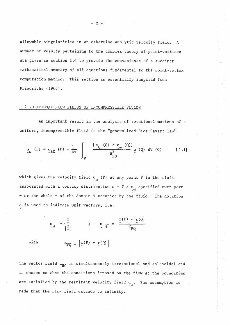
I.2 ROTATIONAL FLOI^I FIELDS OF INCOMPRESSIBLE FLUIDS

An imporEant result in the analysis of rotational motions of a

uniform, incompressible fluid is the ttgeneralized Biot-savart lawt'

u (P) Y¡c (P)(¡)

1

Gv

which gives the velocity fiela u, (P) ar any point p in Èhe fluid

associated with a vorticy distribution o = Y " u, specified over part

- or the v¡hole - of the domain V occupied by Èhe fluíd. The notation

e is used to indícate unit vecËors, i.e.

r(P) - r(Q)e-u)

ü)

tlt RrqeQP

with h r(P) - r(Q)a

The vector field l¡c i" simultaneously irrotational and solenoidal and

is chosen so that the'conditions imposed on Èhe flow at the boundaries

are satisfied by the resulEant velocity fielu lr. The assumption is

made that the flow field extends to infinity.

3

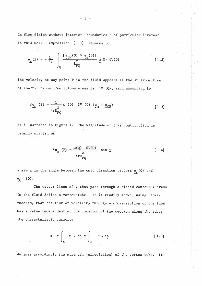
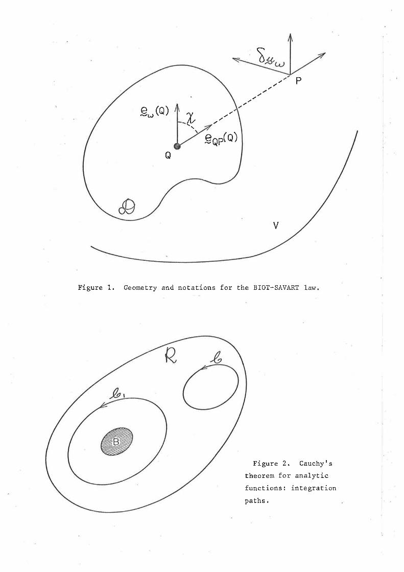
In flow fields without interior

in this work - expression t 1.11

boundaries - of partieular interest

reduces to

Pa) x e,(Q)l

ur(Q) dv(Q) t 1.21

The velocity at any point P in the fLuid appears as the superposition

of contribut,ions from volume elements ôV (Q), each amounting to

ôu 1

1

uñ[ "qr(u

-ü))(

2*rQ

v

- (¡)

as illustrated in Figure I

usually wriÈten as

ôuu)

(P)

(P) =-0) (a) ôv (Q) (3,2

4nRrOQP

xe )

The magnitude of this conÈribution is

[ 1.3]

t 1.41s].n x4nRrO

where ¡ is

iqr (c) '

The vector lines of o that pass through a closed contour .Q, dravnr

in the fluid define a vorlex-tube. It is readily shown, using Stokes

theorem, thaË the flux of vorticity through a cross-section of the tube

has a value independenÈ of the locatíon of the section along the tube;

the characteristic quantity

û, dA= u.ds [ 1.s]

the angle between the unit direction vectors er(Q) and

K=

A t

defines accordingly Ëhe strengËh (circulation) of the vortex tube. It

rP

Figure 1. Geometry and notations for the BIOT-SAVART lav¡

V

Figure 2. Cauchy I s

theorem for analyticfunctions: integrationpaths.

.9- (o)þ,

o

.9qp(o)

4

is clear thaE Èhe cross-section of a tube cannot contract Eo zexo without

Ëhe vorticity becoming infinite; vortex-tubes must, therefore form finite

closed loops, end or begin on boundaries, or extend to infinity.

A vortex-filament of sÈrength r< is a vortex-tube of infínitesimal

cross secEion; it may be visualized as a set, of contiguous cylindrical

vorËicity elements, of length ôL and section o with

i (a) ôv (Q) = (¡) (a) (a) (a)o ðL

=rôL(Q) t 1.61

aligned along a given curve L drawn in the fluid. The velocity fieldt'inducedt' by " vortex-filament is given by equation

dL (Q) X (a)u [ 1.7]

which is a particular form of fL,2l,

Tr,¡o-dimensional flow fields correspond to configurations where

all vortex-tubes are parallel cylinders extending to infinity; the

plane of flow is clearly normal to the direction of their generating

1ínes

Denoting 6A the element of area in the plane of flow, and ôz the

element of length normal to Ëhat plane, one Èransforms [1.2] by writing

ôv (Q) 6A (Q) 6z (a)

and carrying ouE the integraEion wiÈh respecL to Ëhe variable z

The velocity components are nohl given by the expressions

K

GJ.

QPe

(P)K 2

*tQ

1

i^

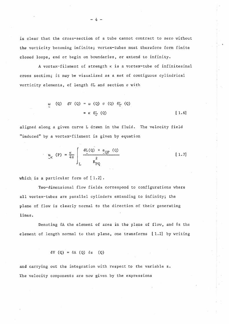
-5-

u(P)=- ñ

1

(t)(Q) dA (Q)

o(Q) dA (Q)

*rQ

and v (P)2n

I^

I r.e]

l l.el

*tQ

The velocity field is known Èo be solenoidal and hence is derivable from

a stream functíon which has the form

1

fo"o' ros nfo dA(Q)

2Rpq

ú(P)= 4r

in view of. [ 1.8] .

The two-dimensional velocity field induced by an infinite,rectilinear vortex-filament is obtained from [1.7] :

u(P)=- K

ñ

[ 1.10]

v(P)= K

ñ(a) I

2

The point Q represents the trace of the filament in the plane of analysis,

and represenÈs a point-vort.ex of strength ¡<. The corresponding stream

functíon is

K

[x(P) - x

*rQ

2{,(P)=- G los hQ [ 1.11]

-6-

The above results may be obtained if a slightly differenÈ point

of view is adopted. The poinÈ-vortex approximation (PVA) generates a

discreÈized form of equaÈions [1.8], t1.91 according to the following

procedure. The vortical area A is broken up into a number NV of small

elements ôA that saEisfy the requirement.

NVA=I ôA(Qc)

ct

Qo being the rrcentret'of element tto,tt. The assumption that each element

ôA (Qo) contracts into a poinÈ-vortex of strength

K 0)

ôA

leads Èo the fundamental formulae

(Qq)

1v (P) 4¡

1(P) 2r

(Qs) ôA(Q0)

NVzx ro loe \oc

=K I t.tzl

[ 1.13]

[ 1. 14]

CI

u v

1v(P)=+ 2r I x (r) - xol /\o

Qo (xo, yo)

2*"o= [ x (P)

lct

NVxq

NV

ly (P)2

/*"o

2L

c,

2

with

and2

x0

+ [y (P) - Yol

It is interesting to point out that the vorticiËy concept, whichís central to the theory of inconrpnessible fluíd motíon, is complementedby the notion of expansion in the general case of contpressible fluidmotion.

7

The ilCauchy-Stokes decomposition Eheoremtt asserEs Lhat "anarbitrary instantaneous sÈate of motion may be resolved at each poinL inEoa uniform EranslaÈion, a dilatation along three mutually orthogonal axesand a rigid rotation of these axes" (Truesdell, L954). This Ëheorem showsclearly that the vorticity g = Y x u - representative of the fluid rotation -and the expansion 0 = Y giving the fractional rate of change in thevolume of a material elemenË - appear naturally as dual variables in theanalysis of the kinematics of continuous media.

The essentíal sígnificance of the distributions of vorticity andexpansion may be otherwise appreciated by considering the Stokes potentialsof the velocity field. IË is a well-known result of vector analysis thatany vector field g, enjoying suitabLe differentiability propert,ies, may beglobally represented as t,he sum of an irrotational field and a solenoidalfield

The scalar function 0 and the vector field A - known as the Stokespotentials of the field c - are noE uniquely determined: the addition of añarmonic function { to tñe scalar poteniial 0 and that of a gradienE termVa to the vector potential A leave t.he above representation unaltered.One possible pair of potentials is given by Ëhe expressions

:0*Y"1

4nu(P)=-rf- -Jv

1

G(v'c)

-dv

r ; -A= (Vxc)

-dv

r104n

V

The double indeterminaÈion can be raísed by selecting a so that$ ís solenoidal, whilst choosing Q so that boundary conditions imposed onc are saEisfied.

One can Èherefore broadly assert that in general, the velocityfield may be represented under the form

0 (o) dv (a) t¡(Q) dv(Q)

*rQhq

(of which [ 1.1] is a particular example).

Vortices and sources are síngularities of the vorticity field andexpansion field respecËively; any (instantaneous) motion may be inducedby an unstable configuration of sources and vortíces. The source-vortexanalogy breaks down however when dynamical considerations are included inthe analysis: vorEices are essentially Lagrangian in character, whilesources are an Eulerian feature of the flow. The difficulcies met in

v

l;*Y*

-8-

attempÈs Eo generalize the poinË-vortex approximation to includecompressíbility effects stem essentially from this distinguishingproperEy, which leads to complex evolution equaËions for the coupledvorticiËy and expansion distributions.

I.3 INTEGRAL INVARIANTS OF TI^IO-DIì'fENS]ONAL VORTICITY DISTR]BUTIONS

All results presented in Section I.1 are essentially kinematical

ín nature: they refer to instanLaneous configurations of the velocity

field and apply aE any gíven instant, irrespective of the dynarnical

aspects of the flor¿. Dynamical considerations are, however, necessary

to establish that the temporal evolution of (two-dimensional) vorticity

distributions takes place in a manner which conserves several integral

quantities. These invarianËs and their physical significance are

examined below.

Kelvínfs circulation theorem asserts that the circulationrI = 0 u . dL round a material line in an inviscíd, incompressible fluidJL -

of uniform density is ínvariant:

TdrE [ 1.15]=0,

provided Ehe body force is derivable from a single-valued potential.

A direct consequence of Èhis theorem for the case of a t¡¿o-

dimensional vorticity distribution extending over a bounded region A is

ÈhaÈ Èhe total circulation

dL= dA I r. ro]I,A

r =f :L

around a closed contour fully containing A is invariant. This invariance

-9-

condition is 1ocally expressed as

d (t¡ôA) = Q [ 1. 17]dr

for a material element of area ô4.

Consider now the time rate of change of the expression

Mv

x t¡l dA [ 1.18]A

which is Ehe first moment of the vorticity disÈribution with respect to

the y axis.

One computes

Mv

ddr (x dA) = i< (odA) + x d

æ (t¡dA)

A A

u (P) rll (P)dA(P) in view of [ 1.17].

Introducing the expression of u (P) from equation [1.8] one obtains

A

t

Mv

12n

dA(P) dA(Q)

AA*rQ

an expression which vanishes identically. The quantitV t't, is therefore

an ínvarianE of the motion; it is obvious that Ehe moment

f^

is also invariant.

Mx yodA [ 1.19]

-10-

The position of the centre of vorticity of the distríbution is

defined in t,erms of l, M* and ",

bt the relations

t{v

I

xt¡dAA

T

t¡l dAA

yûrdA I r. zo]MxT-

Al=r¡ dA

A

provided that I differs from zero. One can also consider that the

vorticity centre is situated aÈ infinity when the total circulation

vanishes

It is easy to show Ëhat the raÈe of change of the quanEíty

J=22

(x +y)urdA [ 1.21]A

is zero. Indeed, one has, using [ 1.17],

2(xu + yv)dA

and subsÈitution of the explicit expressíons of u(P) and v(P) (equations

t 1.81) inÈo Ehe above idenÈity yields

o(P)o(Q)t x(r)yçq¡ - y(P)x(Q)l dA(P) dA(Q) ,

i= IA

j=11f II

A

and finally

The invariant quantity

j=0.

J is identified with the "moment of inertiarr of

-11 -

Ëhe vorticity distribution. It is convenient to introduce a I'radius of

gyration" (or "dispersion lengËh") I by the relationship

t (x-x)2+(y-Y)21, ¿R

L L.221

21. e. (x +Y ).

The inÈegral giving the kinetic energy of the fluíd occupying the

whole plane is not finite. It is however possible t,o derive an invariant

associaËed with the kineËic energy by examining the manner in which the

energy integral over a bounded region Q diverges when letting ll tend

to infinity. Consider the kinetic energy of the fluid (*) wittrin the

region O, taken as a circle of large radius R toLally covering the

vorticity domain A:

T =tÁ' (u +v )ao

One transfor¡rs T as follows with the use of Stokes theorem:

IA2

It¡ldAI

A

JTI

22

0

22

T=1Á' I0

t"#- "#) un

=,ÁlA

,|tu dA, - 1râ

Jr k,"r, - for",r,> tç¿

do

=l! þu dA. - lL f v :.d: , [ 1.23]

af¿A

(*) Assuming unit density for simplicity, i.e. usíng the kinematicaldes cription.

-L2-

where AA is the circumference of radius R limiting the region A.

LeEting R Èend to infinity, one compuËes the conÈribution from the

line integral as

2n{(R)uu RdO

2tt

l**'u==

1

R

I0

ío

T+

r-ft tog ( 1It 2¡rR

Rd0

* los (å) (n+-¡

The asymptotic form of expression I L.23) for R + - may be writ,ten

¡2G log I r.241

The kinetic energy of the fluid is conserved in the absence of dissipation;

the left hand side ot lL.24l is therefore independent of time, a property

which establishes the invariance of the quantiÈy

[ 1.2s]

An alternative expression for H - called the Hamiltonian of the

vorticity disÈributíon, for reasons exposed in section I.4 - is obtained

by substitution of equation [ 1.9] into equation [ 1,251, yielding

H=-# 1og 4q uolt¡ dA(a) (* ) I L.261

(*) His also called the "Kirchhoff function" of the sysÈem of vorËices;both names will be used in Èhis work.

dAtþtrt(+)='al.A

H=rL f t'ooA

a)J f ',',',AA

-13-

There are several ways of establishing the expressions for the

invariant quantiEies associated with the motion of a collection of

isolated point-vortices. Inspection òf the definirion integrals for

f, X, Y and 12 suggests, in víew of relation [1,L21, that the discrete

counterparts of expressions [ 1.16] , I r.zo] and I L,22) are respectively

NVI=X

0

NVl\- L

d

K Í r,271c

rcx/rc ct'

[ 1.28]J=

t12 rol (xo-x)2 + (ro-v¡21 I L.zel

The expression for the discrete Hamiltonian must be determined

somewhat more carefully due Ëo the singular character of Èhe kineËic

energy of a poínt-vortex. IË is necessary to consider, as for the

continuous case, the kinetic energy T of the fluid within a circle of

large radius R, and outside small circles of radius e cenÈered on each

point-vortex. One shows that Ëhe following relationship holds asymptotí-

cally as R+- and e->0:

T+ I4t¡

1og R

-> [ 1.30]

"*Yo/ f

NVx0

NV

c

rY"å) roe ,-+(Y",)'do

1oB Raßx

B*axd

*o"ß

analogous Èo equation [ 1.241 ,

1

G

This identity, establishes on sinilar

-14-

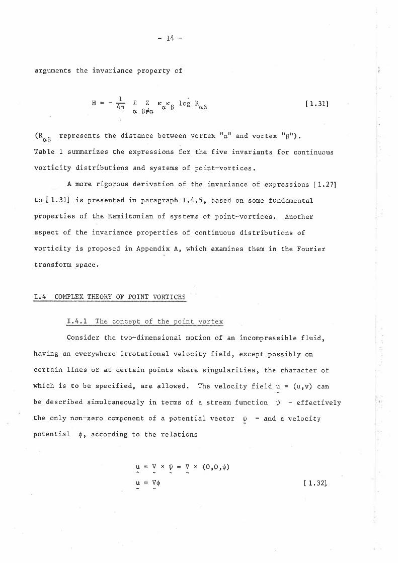
arguments Lhe invariance property of

u=-l4T1 "o"ß

1og RaßL

cL

ß#e[ 1.31]

(R*ß represents the distance between vortex "cltt and vortex t'ßt').

Table 1 summarizes the expressions for the five invarianÈs for continuous

vorticity distributions and systems of point-vortices.

A more rigorous derivation of the invariance of expressions ÍL.271

Èo [1.31] is presented in paragraph I.4,5, based on some fundamental

properties of Èhe Hamiltonian of systems of point-vortices. Another

aspect of the invariance properties of continuous dístributíons of

vorticity is proposed in Appendix A, which examines them in the Fourier

transform space.

T.4 COMPLEX THEORY OF POINT VORTICES

I.4.L The concept of the point vorËex

Consider the two-dímensional motion of an incompressible f1uid,

having an ever) ¡rhere irrotational velociÈy field, except possibly on

certain lines or at certain points where singularities, the character of

which is Èo be specified, are allowed. The velocity field u = (urv) can

be described simultaneously in terms of a stream function r! - effectively

the only non-zero component of a potenÈial vector rf - and a velocity

potential 0, according to the relations

(o ,O , rr):=Y't=Y"v0u I r. ¡z]

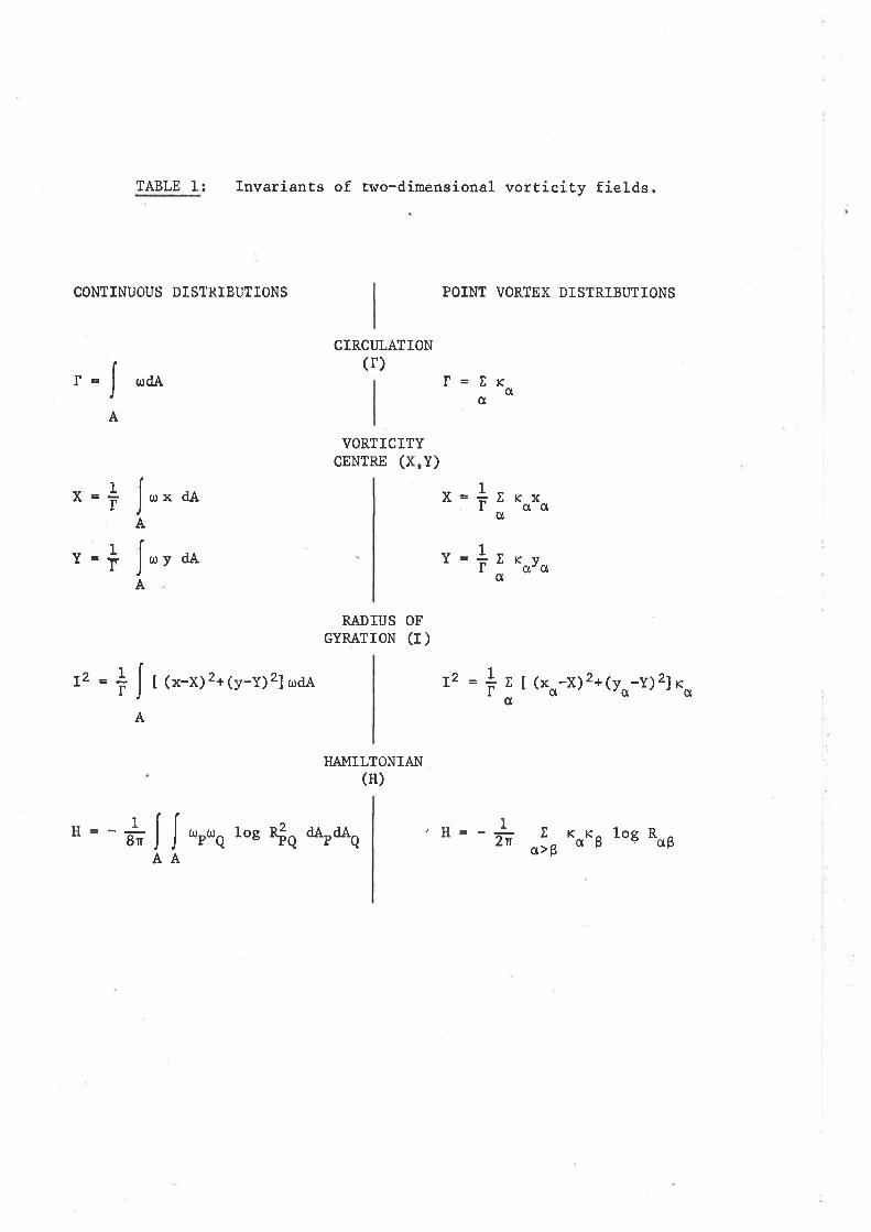
TABLE ].: Invariants of two-dimensíonal vorticiËy fields.

CONTINUOUS DISTRIBUTIONS POINT VORTEX DISTRIBUTIONS

CIRCT]LATION(r)

t¡ldA

A

1v-r\- T

1l= T

H=-Btt

opûrQ los *lq *ruoq

VORTICITYCENTRE (X,Y)

RADIUS OF

GYRATTON (r)

HAMILTONIAI{(H)

I=Erc

'/H=- 1

o

dA

dA

J,-A

J,, 'A

r, = * | f <*-xl2+(y-y)2lr¿¿,

A

x=lxrxl' od0

Y=+r"oroo

t, = + x [ (xo-x)2+1yo-y)2lrot

IIAA

1

ñ o36 *o"ß 1o8 Roß

l

I

I

-15-

The scalar functions 0 and rf are related by equations of the cauchy-

Rieuann type:

allowing the analysis to be pursued in terms of the analytíc function

aü= â0ðy ðx

x(z)

avâx -?-0

ðy

0+iv

The complex veloeity w(z)

contains bodies (see Figure

[1.33]

[ 1.34 ]

is clearly

2), rhe

of the complex variable z = x + iy; XQ) is the complex poËential of the

flow. The eomplex velocity field

w(z)=u*iv [1.3s]

is obtained by differentiating X(¿) with respecÈ to its argument:

#.t**='*(")x'(z) =u-1v= I r. goj

(starred quantities represent complex conjugates). Cauchyrs theorem for

analytic functions staÈes that

fc

f(z)dz = Q

in a domain dì and any simple closedfor any function f(z) analytic

contour C completely within ft.

noÈ analyric in a domain dì that

complex circulation

[ 1.37]

around any closed curve encircling a body does no! vanish and one has

generally

dz(z)\nt*z={c

-16-

wr(z)dz = r + i ,

where

and

(udx + vdy) d0

drll(udy - vdx)

The complex circulation reduces to its real part if no sources (sinks) are

present, within Ehe region liurited by the contour C; it hrill be assumed

hereafter that this condition is realized (í.e. ¡\ = O).

Suppose now that the cross-section of the body is made to shrink

to an infinitesimally smal1 circle, all other flow conditions remaining

unaltered. The body becomes a punctual singularity of the flor¿ field,

such that,

[ 1.38]

for any closed contour drav¡n around it: the singularity defined by this

limit process is a point-vortex of strength K. Any velocity fieLd of

the form

w* (z) K

2h(z-ç) + w[(z) [ 1.3e]

(rc real)

r^rhere w[(z) is analyÈic at z = Ç, comprises a point-vortex of st,rength

K at z = Ç, as shown by a direct application of the residue theorem when

evaluating the corresponding circulation around a curve enclosing the point

z = ç. The complex potentíal associated with t1.39] has the form

y(z)=* Ioe(z-Ç) +x*(z), [1.40]

z=lc

=fc

=fc

"=fc

^=fc

IZ=Avf(z)dz=rJ

c

-17-

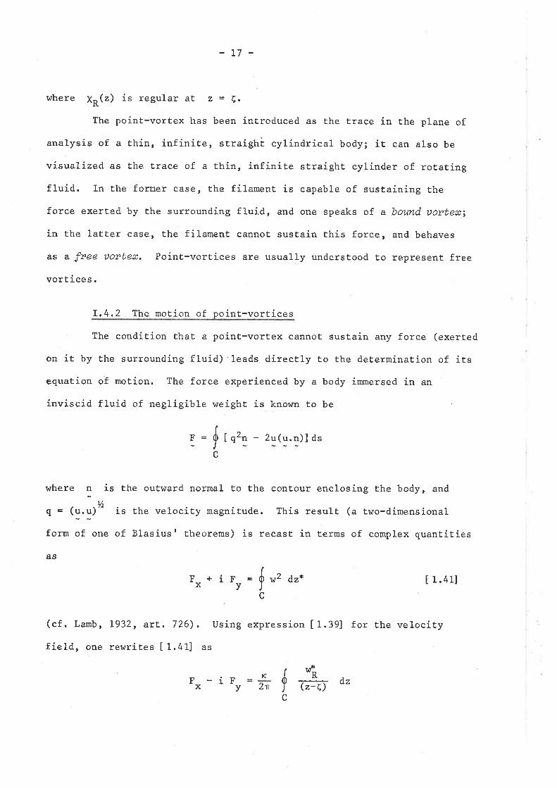
where X*(z) is regular at z = Ç,

The point-vortex has been introduced as the trace in the plane of

analysis of a thin, infinite, straighÈ cylindrical body; ít can also be

vísualized as the trace of a thin, infinite sËraight cylinder of rotating

fluid. In the former case, the filament is capable of sustaining the

force exerted by the surrounding fluid, and one speaks of a bound tsorteæ;

in the latter case, the filament cannot sustain this force, and behaves

as a free Ðovteæ. Point-vortices are usually understood to represent free

vortices.

T.4,2 The motion of point-vortices

The condiÈion that a point-vortex cannoÈ sustain any force (exerted

on it by the surrounding fluid)'leads directly to the determination of its

equation of motion. The force experienced by a body immersed in an

inviscid fluid of negligible weight is known to be

I q2t - 2u(u.n)] ds

where n is the outr'¡ard normal to the contour enclosing Èhe body, and

uO = (u.u)'- is the velocity magnitude. This result (a two-dimensional

tot* lf one of Blasius I theorems) is recast in terms of complex quantities

AS

[ 1.41]

(cf. Lamb, L932, ar|. 726). Using expression [ 1.39] for the velocity

field, one rewrítes [ 1.41] as

K-ä

r=fc

F +iF =[r'dr*xy)c

6fc

F -iFvx 2n

dz

-18-

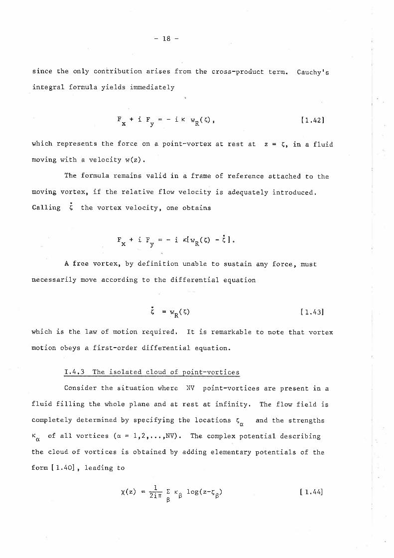
since the only contribution arises from t,he cross-product term. Cauchyrs

integral formula yields imrnediately

v IL.42l

which represents the force on a point-vortex at rest at z = e, ín a fluid

moving wíth a velocity w(z).

The formula remains valid in a frame of reference at,tached to Èhe

moving vortex, if the relative flow velocity is adequately introduced.

Calling f tft" vortex velocity, one obtains

F +iF I r<[ v¡*( E)x v

A free vortex, by definitíon unable t,o sustain any force, must

necessarily move according to the differential equat,ion

F + i F = - ir w*( 6) ,x

- ir

which is the

motion obeys

r.4, 3 The isolated cloud of point-vortices

Consider the situatíon where NV poínt-vortices are present in a

fluid filling the whole plane and at rest at infinity. The flow field is

completely determined by specifying the locations 4a and the strengths

"o of all vortices (cl = 112r...rNV). The complex poÈential describing

the cloud of vortices is obtained by adding elementary potenEials of the

form [ 1.40] , leading to

"ß)

E =w*(Ç) [1.43]

law of motion required. It is remarkable to not.e Ëhat vortex

a first-order differential equation.

1x

ß

xþ) 2ir Iog(z-çB

I L.441

-19-

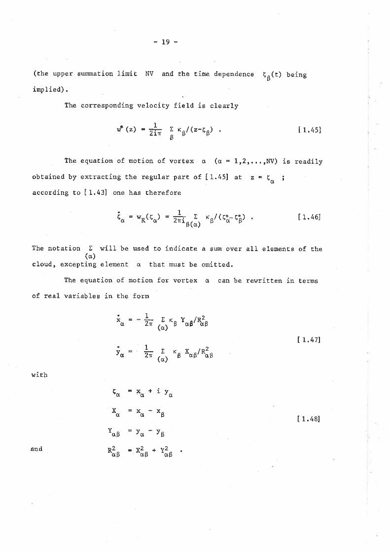
(the upper sunmation límit NV and the time dependence qo(t) beingp

implíed)

the corresponding velocity field is clearly

I[ 1.45]vf (z) = ffi

The equation of motion of vortex q, (o = 1 12¡...rNV) is readily

obËained by extracting the regular part of [ 1.45] aE , - Ça ;

according to [1.43] one has Ëherefore

I *

ut @-Es)

[ 1.46]

The notation I will be used to índicate a sum over all elemenEs of the(a)

cIoud, excepting element cl thaÈ must be omíËted.

The equation of motion for vorËex o can be rewritten in terms

of real variables in the form

io = '*(Eo) = #u,j, rul(e¿-rþ)

/Rls1

ñx1l¡"0

Yoe

h ,i, "s xoo/RÍoa

v

o

CT

Í L.47J

[ 1.48]

with

gc x +iv'0

x =x0t ßd

x

Yaß =Yo-rß

Rfis =*3e*\âsand

-20-

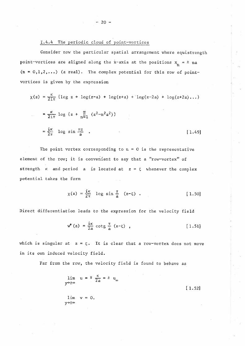
I.4.4 The periodic cloud of point-vortices

Consider now the parEicular spat.ial arrangement. r¿here equistrength

point-vortices are aligned along the i-axis at the positions xr, = t na

(n = Orlr2r,..) (a real). The complex poEential for this row of point-

vortices ís given by the expression

xG) ffi {Iog z + log(z-a¡ + 1og (z+a) + Log(z-2a) a logQ+Za)...\

= Zfr 1og {, * ,,Er Q2-n2a2)}

K

irñ

ltza

log sin [ 1.4e]

[ 1.50]

The point vortex corresponding to n = O is the representative

element of t.he row; it is cotrvenienË to say that attro$¡-vortext'of

strength r and period a is located at z = Ç whenever the complex

potential takes the form

x(z) 1Kñ

fiIog sln - (z-e)

Direct dífferentiation leads to the expression for the velocity field

ulÈ (z) 1KE"o [ 1 . s1]

which is singular at z = Ç. It is clear that a row-vortex does not move

in its own induced velocity fíeld.

Far from the row, the velocity fiela is found to behave as

lin u=TY+t-

K

ñ

lim v=0.v->+o

q n G-e) ,

=t uæ

t t.szl

Çg

-2L-

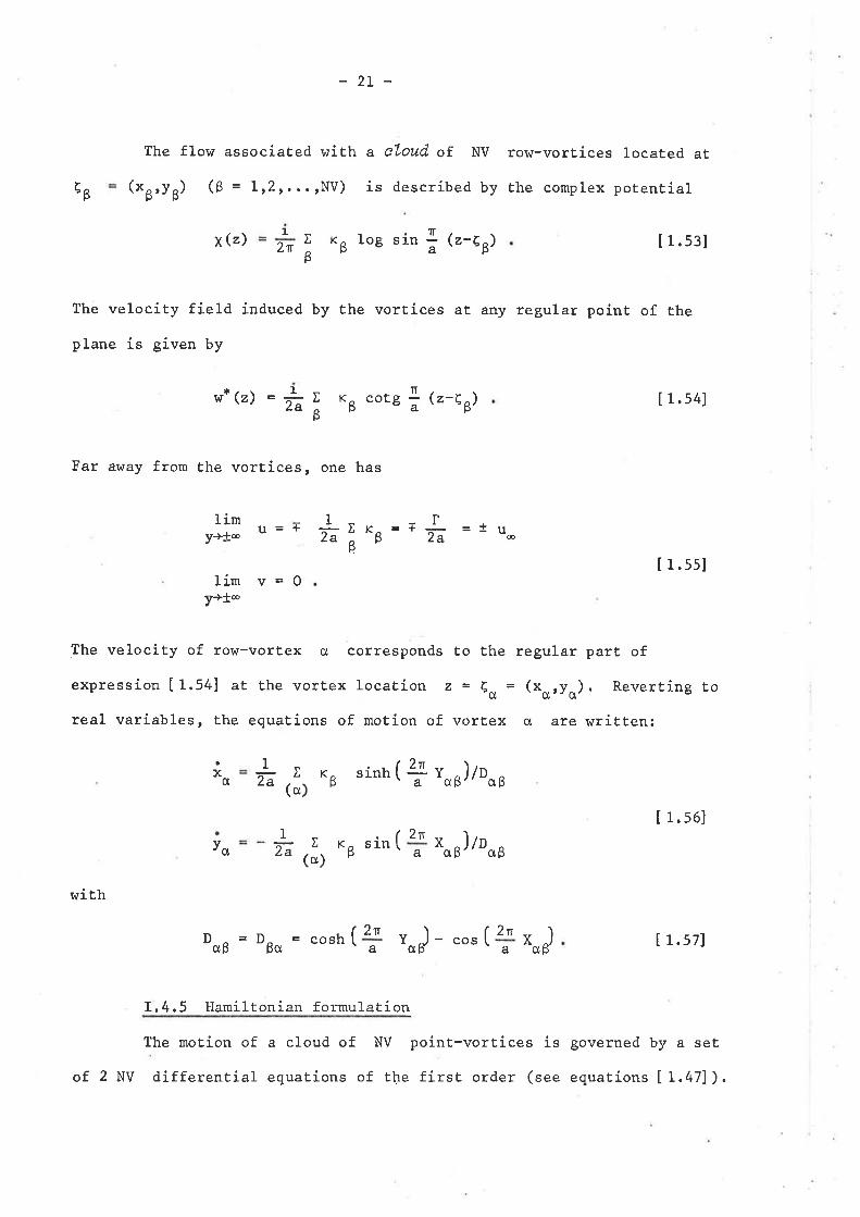
The flow associated with a cLoud of. Nv row-vorEices located at

(x'rf') (Ê = 112r,,.,NV) is described by the complex potentíal

x (z) v

Ê

tog s in !" e-e U) [ 1. s3]

The velocity fiela índuced by the vortices at any regular poínÈ of Ëhe

plane is given by

hr* (z) 1

ñ Iß

r<ß cots I Q-e g) [ 1.54]

one has

1

2r Kß

Far away from the vortices,

limv->+@ U=+ T1E =tu

ä*u=* ñ[ 1.ss]

lim v=Ov++æ

The velocity of ro\^r-vorEex o corresponds to the regular part of

expression [ 1.54] at the vortex location " - Ça = (xcrryo). Reverting to

real variables, the equaÈions of motion of vortex o are written:

sinn ( * "ru)/oou1x

o ñ Xr( cr)

Ir sln )to

æ

2r

ß

[ 1.s6]I 2r(Ycr 2a g

(a)

D =f = cosh

a ßX

0 oß

with

2n( vo] - "o" I JclÊ Bcl aX [ 1.s7]

f,4.5 llamiltonian formulation

The motion of a cloud of NV point-vortices is governed by a set

of 2 NV differential equations of the fírst order (see equations t1.471).

ct4

-22-

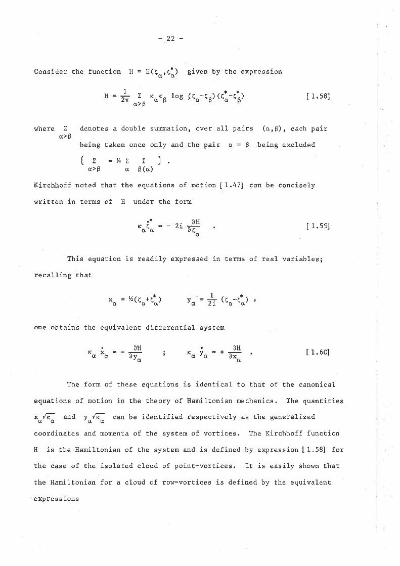
Consíder the function tt = H(çarÇl) given by Ëhe expression

1 *o*ß roe (qa-çß) cei-ril

AHq

rC

L-cr )"o

= * tro-dl

[ 1.58]

(cr, ß) , each pair

being excluded

can be concisely

[ 1.60]

}{= ño ß

where X denoÈes a double sumniation, over all pairsq>ß

being taken once only and the pair q = ß

( r ='ÁE x )cr>ß a ß (q)

Kirchhoff noted that the equaËions of motion IL.47]

written in terms of H under the form

x

K =-2L t 1.sel

This equation is readilg' expressed in terms of real variables;

recalling Ehat

Ç

t

oo

xc = t5(Ç +c

one obtains the equivalent differential system

K =+"o IoAH ÐHr

oo

The form of these equations is identical to that of the canonical

equations of motion in the theory of Hamiltonian mechanics. The quantities

x^.fi and y^.8 can be identifíed respectively as the generalized0 c -ct ct

coordinaÈes and momenta of the system of vortices. The Kirchhoff function

H is the Hamiltonian of the system and is defined by expression [1.58] for

the case of the isolated cloud of point-vortices. It is easíly shown that

the Hamiltonian for a cloud of row-vortices is defined by the equivalent

expres s ions

Yodv

-23-

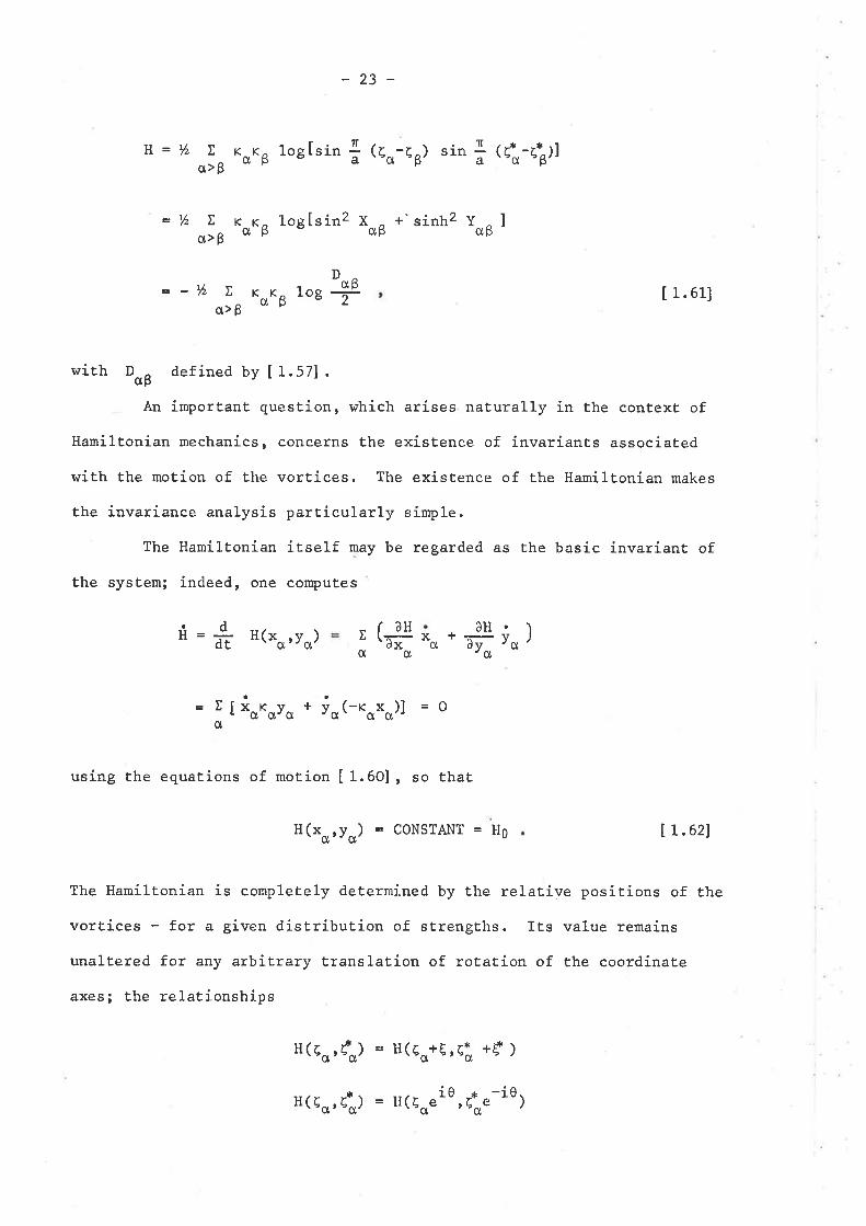
H=lâ X r r^a>ß aþ 1ogIsin ] (eo-eu) sin I {ri-eill

ß1og[sín2 xo' +'sinh2 YoB ]

- DoB

"o*ß to8 T

=l! X ro>ß

= -15 [a>Ê

Ko

[ 1.61]

with D-.^ def íned by [ 1 .571 .0Þ

An important question, which arises naturally in the context of

Hamiltonian mechanics, corlcerns the existence of invariants associaÈed

wíth the moËion of the vortices. The existence of the llamiltonian makes

the invariance analysis particularly simple.

The Hamiltonian itself may be regarded as the basíc invariant of

Ehe system; indeed, one computes

ú = + H(xo,Io)-Xdx ct

+ ðv rcrAH( âH

)x0

x Iio*oyo + lo(-roxo)l

0

=Qc

using the equatíons of motion I f.0O], so that

H(xoryo) = CONSTAÌ{T = H0 L L.62l

The Hamiltonian is completely determined by the relaÈive positions of the

vorËices - for a given disÈribution of sËrengths. IËs value remains

unaltered for any arbitrary translation of rotaLion of the coordinate

axes; Èhe relaEionships

H(Eo, å) = H(ç'+t, Eå *d )

H(6a,8:) = H(Eo"io,{"-tu)

-24-

hold for arbiÈrary values of the consLanÈs

These identities are equivalent Èo

t = o + iÊ and 0.

the three conditions

âHlaol

E=o=Q ;

alternatively expressed as

=QAHr

dx =âH = odvct

âHl

-tâßlE=oAH

=Q;a0 =Q ,

0=O

e-(IâH

ãr-ct(ro AH

)to

xo

Ëal"f= X rCTo

IJ2=Xrc r r*cro'o-0

) ãr-c[=Q

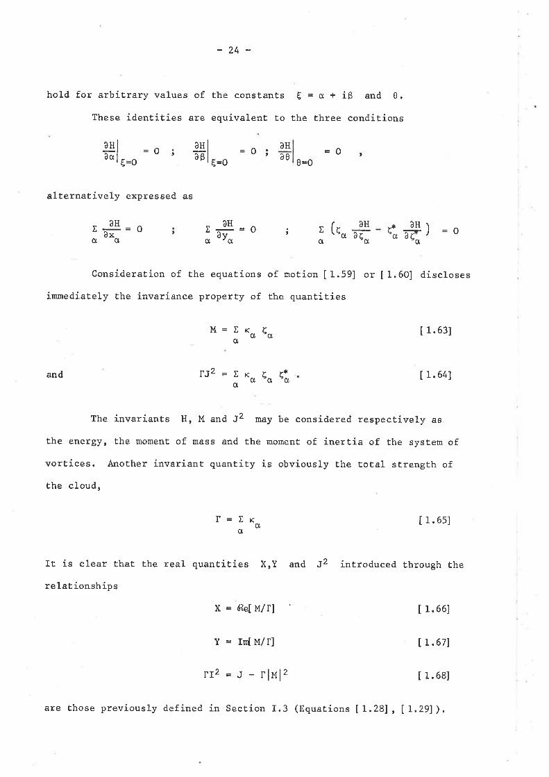
Consideration of the equations of motion [ 1.59] or [ 1.60] discloses

irnmedíately the invariance property of rhe quantities

[ 1.63]

and [ 1.64]

The invariants Il, M and J2 may be considered respectively as

the energy, the moment of mass and the moment of inertia of the sysLem of

vorËices. Another invariant quantity is obviously Èhe total strength of

Èhe cloud,

l=Xr [ 1.6s]qct

It is clear thaL the real quantities XrY and ¡2 inËroduced through the

relat ionshíps

x = GelM/rl t1.661

y = rn{ ¡llll f L.671

rr-2 =.r - rlul2 [ 1.68]

are those previously defined in Section I.3 (Equations [ 1.28], IL,29]),

-25-

I.5 ST]MI,fARY

Chapter I is íntended as an ttaide-mémoírett that covers succinctly

several aspects of point-vortex theory. It emphasízes the kinematical

significance of poínt-vorËíces, outlines the important invarianee

propertíes of two-dimensional vorticity distributions and enumerates

most of the equations that are needed in the poínt-vortex approxímation

method.

Applícations of the method of point-vortices are considered ín

Ëhe following chapters.

CHAPTER II: THE CENTRN-TO-CENTRE POINT VORTEX APPROXIMATION

INTRODUCTION

THE POINT-VORTEX APPROXII"ÍATION

IL.2.1 Outline of the method

II.2.2 Tl:re development and substance of the PVA

THE CLOUD DISCRETIZATION APPROACH

THE CENTRE-TO-CENTRE METHOD

EFFECTS OF INTEGRATION PROCEDURE, TIME STEP ANDCELL SIZE IN THE CTC METHOD

II. 1

TT.2

II.3

TT,4

II.5

Rankine ts vortex

The PVA of Rankine I s vortex

Eulerrs integrat,ion nethod

Huenrs (Euler modified) integration method

Víscous decay of a vorticity disk

The evaluation of H (t) and of dH(t)/dt

Viscosity estimaÈes

Discussion of results

TT.7 THE ROLLING-UP OF A VORTEX SHEET

rr.5 . 1

rT.5.2

rr.5 .3

rr.5.4

II. 6 VISCOUS EFFECTS IN THE CTC METHOD

rr. 6. 1

TT,6,2

rr. 6.3

rr. 6. 4

rr.7 . I

rr.7.2

SIJM}4ARY

lJes twater I s ro ll-up prob lem

The Cloud Discretization Approach

II. 8

-26-

CHAPTER II

THE CENTRE TO CENTRE POINT_VORTEX APPROXIMATION

II.1 INTRODUCTION

The purpose of this chapter is to inËroduce the computation method

developed for the numerical sËudies of two-dimensional, rotational flows

presented ín this thesis. The method is an original implementation of the

point-vortex approximation detailed ín ChapEer I.

The propert.ies of the proposed vorÈex-tracing algorithm are care-

fully examined by comparing compuÈed flows with two simple, exact reference

flows. Rankine's combined vortex (the disk of uniform vorticity) is first

considered in order Èo determine the limitations and accuracy of the method

used here and Èhe nature of the "viscoustr effects inherent in the computation

procedure. The rolling-up of an el1iptical1y loaded vortex sheeÈ (trlestwaterrs

problem) is then investigated to further assess the capabilities of the

method, and to vindicat,e its use when information about large-scale aspects

of the flow is sought.

Throughout Lhis chapter, aËÈenEion is focused on the behaviour of

the invariants that characteríze the motion of a two-dimensional inviscid

vorticity field. It is found that the invariants - in particular the

Hamiltonian or Kirchhoff function - can be used to moniÈor the accuracy of

the computation; this is in contrast with most applications of the point-

vortex approximaÈion reported in the literature, in which various arbiÈrary

numerical resEraints have been applied v¡ithout assessmenE of their effect.s

on the invaríants of the motion and on the consequent accuracy.

IÈ is argued that the method is therefore capable of providing

-27-

adequate I'statisÈicalrr information about two-dimensional, rotational

ínviscid flows - which is proposed to be relevant to high Reynolds number,

free turbulent flows - in terms of quantitative estimates of parameters

associat,ed with the large scale motions.

The beating of the present. results on some implementations of the

point-vortex approximation reported in the literature is briefly discussed.

IÈ is felt that the infornation obtained here gives additional insight into

Ehe somewhat controversial point-vortex method, whilst suggesting a new

atÈitude towards further developments of the technique.

TT.2 THE POINT-VORTEX APPROXIMATION

IL2.1 Outline of the method

Two-dimensional motions of inviscid, incompressible and homogeneous

fluids are governed, when analysed in terms of the vorticíty field o(xry,È),

by the non-linear equations

v2,1,=-' ; Bi =e t2.11

where rl(xryrt) represents the stream function and ,+ denotes

differenÈiation following the moËíon. These equations are satisfied in

some domain úì of the plane, limited by a contour âß, where appropriate

boundary conditions apply.

The structure of the differenÈial system l2.ll reveals the cenËral

role played by the vorticity distribution in the dynamics of the flows

under consideration. Clearly, knowledge of the vortícity distribution at

some instant determines completely the current and subsequent configurations

of the velocity field (subject to the constraints imposed at the boundary

âû.). Furthermore, and in contrast to its active part as "source" of the

28

motion, the vorticity remains attached to the fluid particles and is

transported during the motion as a passive, scalar quantity.

Several discretization schemeb are available t.o the numerical

analyst in order to solve the differential problem t2.1]. Among possible

alternatives, the point-vortex approximation (PVA) remains particulaïly

appealing due to its simplicity, its suitability for conìputer analysis,

and its flexibility in providing direcÈ visualizaEion of flow patÈerns.

For the reasons given be1ow, a new implementation of the PVA has been

developed and used throughout this work to conduct a number of numerical

experiments.

In essence, the PVA replaces Èhe continuous vorticity distribution

by a system of discret,e, interacting point-vortices. The principle of

the discreÈization may be t"pt.""tted as follows. The rotational region

of the flow is divided into a large number of small elements (the fluidttparticles"), each of which carries a certain amounÈ of vorticity. The

circulation around each element boundary has therefore a non-zero value

that is readily evaluated. Each elemenË is then assumed to shrink about

its vorticity centre, whilst retainíng the value of its circulation. This

limit process defines clearly the location and strength of the point-vortex

that represents the element in the final discretized system. The fl-ow

evolution is then depicted by the motion of the set of point-vortices.

Each point-vortex interacts instantaneously wíth every other vortex by a

simple action-at-a-distance 1aw; it moves accordíng to the local value of

the velocity field whilst simultaneously contributing to the motion of all

other vortices. The trackíng of the vortices requires in principle the

numerical integration of a sysÈem of ordinary, non-línear differential

equations that present the remarkable property of forming a Hamiltonian

-29-

system. The system is knornm to possess kinematical invarianEs which can

be used to monitor the accuracy of the numerical computation.

The simplicity of the PVA isr'however, decepËive and masks parÈially

unresolved questions, some of which will be briefly outlined in the following

paragraphs; ËentaÈive solutions will be proposed 1aÈer in the analysis.

Most problems ín the PVA arise from the elimination of the notion

of material area physically associated with each point-vortex. With this

geometrical element removed from the analysis, some flow aspects can no

longer be accounted for, nor represented adequately; for example, the

relationship between disÈribution of vortices and vorticity field is not

uniquely determined.

Finite-area vorticity elements which are f.ar aparÈ (their

separation being gauged in t,erms of a length representative of Èheir linear

dimensions) interact almost as pointwise elements. As they approach one

another, their interactions become more complex with the increasing

influence of finite area effects; local distortions of the velocíty field,

leading to deformations of the cores, cannot be ignored for neighbouring

elements and must be included in a rigorous analysis, Self-induced

deformations nay naturally occur and should also be considered. One musL

therefore note ÈhaË the inability of the PVA method to cope with such

phenomena may lead to physical inconsisÈencies (*). The importance of

these flow features, and the magnitude of the error made in ignoring them

have not previously been adequaEely estirnated.

Additional difficulties arise from the singular character of the

velocity field at the poinÈ-vortex itself. For numerical reasons, this

(*) for example, material lines initially formed of distinct fluid particlesmay occasionally cross - a physical impossibility.

30

singular behaviour is usually removed by some ad-hoc meEhod, which often

consists in approximating the velocity field in the vicinity of the vortex

by that due to a vortex with a finite'(circular) cross section. This

arÈifice of computaÈion, which relies on numerical intuition for deter-

mining a suítable core dimension, does not restore the original concept

of the material vorticity element, and ignores Èhe additional problems

caused by the introduction of finite-area vortices.

It is here appropriaEe to place these problems r¿ithin Lheir

historicaL perspective. The following section presenEs a brief chrono-

logícal survey of the evolution of the point-vortex method, provides a

comparative background for the present method and discusses some of the

solutions to the quesLions raised previously.

II.2.2 The development and substance of the PoinÈ-Vortex

Approximation

The idea of representing a continuous vorÈex sheet by a number of

discreÈe, ttelementalrr vortices, the temporal motion of v¡hich is followed by

a numerical-, step by step procedure, r,ras fírst proposed by Rosenhead (1931),

in his study of the progressive deformation of the unstable interface betrveen

two parallel sEreams of fluid moving in opposite directions. Rosenhead

considered an initial sinusoidal disturbance y(x) = A0 a sin(Znx/a),

discretízed by NV row-vortices of equal strength r = aAU/NV, uniformly

distributed over one wavelength. Although Ëhe number of vortices used was

very limited (NV = 12), Rosenhead was able Ëo demonstrate the smooth

rolling up of the vortex sheeË, accompanied by the periodic concentration

of vortices at intervals equal to the wavelengÈh of the original perturbation.

The smallest Ëime sËep used in this calcuration had the magnitude

AT = 0.25a/LU; the integration scheme used Eulerts method.

-31 -

Among naLurally occuring vortex sysÈems, Èhe trailing vortex sheet

produced by an aerofoil is of obvious importance. The PVA was employed in

this context by Llestwater (1935), to btudy the rolling up of a vortex sheet

of finite breadth, t,he two-dimensíonal idealization of the wing-tip vortex

system. The sheet was found to roll-up smoothlA, at a predicEable rate, in

accordance with the spiral struct,ure predicEed analytically by Kaden (1931).

However, it was noE until the advent of modern computers that the

full capabilities and difficulËies of the method were to be extensively

explore.d, by allowing a finer discretization of the vortex sheeÈ and the

use of higher-order integration schemes, together with much smaller t,ime

s Ëeps .

The possibility of a smooth roLL up of Èhe sheet, in the absence

of viscosíty, was first questioìed by Birkhoff & Fisher (1959). Their

refined version of Rosenheadrs calculat,íons revealed a yqndom trend in the

motion of the vortices, and the development of an irregular, contorted and

physically unrealistic geometry of the interface, ín total conflict with

the smooth, regular pattern of the orígina1 calculations. However, vortices

were found to cluster, which, according to Birkhoff, does no! necessarily

reflecÈ a genuine concentration of vorticiEy: the Hamiltonian associated

with a system of vortices is a suitable measure of the concentration and

is an invariant of the motíon. The ultimate randomness of the distribution

of the vortices r¿as also advocated by appealing to the applicability of the

ergodic theorem for Haniltonian systems (Birkhoff , L962).

The calculalions of Westwater were reconsidered by Takami (1964)

and Infoore (I97I) who were both unable to reproduce the original results:

the smooth spiral structure was again desÈroyed by the same chaotic motion

of the vortices as that showed by Birkhoff and Fisher. The possibility

32

that this chaotic motion was due to the numerical meEhod failing to

integrate the equaËions of motion correctly was ruled ouE by the findings

of Moore: if the Eime step is chosen to be much smaller than the orbital

period of the two closest vortices, the equations of motion are integrated

correctly. One is therefore led to conclude that Èhe exacE solution in

the PVA does noË converge to the solution corresponding to the continuous

vortex sheet; increasing the number of vortices v/orsens the situation. A

saÈisfactory explanation for the emergence of a chaotic motion in the

rolled-up portion of the spiral is provided by the possibility that

vort,ices belonging to dístincÈ turns of the spiralr may come very close

together and generate unrealistically large interactions that eventually

disrupE Ëhe smooth evolution of-the system (Moore, L974). The correctness

of this explanation is supported by the success met by several techniques

in eliminating this random behaviour of the vortices, all of which prevent

any Ëwo vortices from approaching one another too closely, hence suppressing

the occurence of excessive induced velocities. The methods used differ

from author to author. Nielsen & Schwind (1971) substitute, for two

vortices closer Èhan some threshold disÈ,ance, a single equivalent vortex

located at the vorticity centre of the critical pair. Chorin & Bernard

(L972) introduce point-vortices having a smal1, fínite radius core which

ensures the boundedness of the velocity field everywhere in the plane. A

similar technique is adopted by MiliÍLazzo & Saffman (L977 ) and by Acton

(L976)., Kuwahara & Takami (1973) employ the velocity fieta associated with

a díffusing line vortex to the same effecE. They also note that the

coefficient of viscosity appearing in their equations eharacLerizes an

artificial viscosiËy rather than a genuine, molecular viscosity.

Another, more rigorous, explanaEion for the development of a

random motion of the vortices is given by Fink & Soh (L974), who show that

-33-

the PVA of a periodíc, conÈinuous vortex sheet neglecËs the self-

induced velociEy of vortex-sheeË segments that must be included in a

correct discretization of the Biot-Savart integral. Inclusion of higher-

order Eerms in the approximatíon of the integral equaEion for the ellip-

Eically loaded vortex sheeÈ is shown to lead to calculations which converge

as the discretization is refined, and which predict a smooth rolling up of

the sheeË into the expected spiral sEructure (Fink & Soh, 1978).

Many other applicaÈions of the PVA have been reported in the

literat,ure, but are not discussed in detail here; they ínclude studies of

the temporal interacËions between periodic vortex sheets of oppcsite

vorticity - a simple model for the formation of a wake behind bluff bodies

(see Abernathy & Kronauer, 1962> and analyses of the spatio-temporal

development of shear layers sheà fto* bodies placed in transverse flows.

Problems belonging to the second category involve the additional complexity

of boundaries. An extensive and excellent survey of related work can be

found in Clements & Maull (1975).

Some auEhors have been primarily concerned with the computational

aspects of the PVA. The easiest numerical implementation of the method

consists of a direct evaluation of the velociEy of each vortex by summing

the separate conËributions of all other vortices present in the f1ow.

Clearly then, tracing the motion of the whole population requires, at

each time step, a computing effort that, scales with the square of Ëhe

population size, NV2. It is clear that this summation algoríthm

rapidly becomes expensive in terms of computing cost, even f.or a moderate

number of vortices. The situation r"¡orsens if higher-order numerical

schemes are employed for Ëhe inLegration of the equations of motion.

An alternative method evaluates the velocities of Ehe vortices via

the sËream function, and the velocity field. A fast Poisson-solver is

34

used to determine the values of t.he stream function at Èhe nodes of a

rectangular mesh defined over the spaEial area of interest. The vorticity

field is prescribed as a set of discròte mesh-point values, obtained by

redistributing the contributions of the vortices within a cell to its four

nodal points. The velocity field is then computed from the stream function

field values, leading in turn to the velocities of the vortices. This

approach consÈitutes the basis of the cloud-in-ce11 (CIC), particLe-in-ce11

(PIC) or vortex-in-cell method (VIC). The technique was pioneered in the

context of plasma physics, and extensively applied to hydrodynamical

problems by ChrisEiansen (1973). The ability to rapidly solve Poissonrs

equation originates from numerical algorithms akin to Fast Fourier Transform

meÈhods. These meËhods present, however, additional uncertainties linked

with the variety of possible choices in mesh sizes and interpolaËion

procedures required to switch back and forth from an essenEially Lagrangian

description to the Eulerian description over the computation mesh. The

necessity of solving Poissonts equation implies thaË boundary conditions

be imposed over all domain boundaries; conditions ttat infinity" must

necessarily be imposed at fínite distances, leading to possible limitations

of the method. Different codes must also be developed to allow for various

types of boundary conditions (Dirichlet or Neumann; periodic or non-

periodic) .

The possibility of usíng the summation algorithm in the PVA is

often subordinaÈe to the availability of low cost computing resources. A

nev/ vortex traeing scheme, based on a fast version of this algorithm, hTas

developed, with the intenÈion of applying it to the study of two-dimensi.onal

vorticity layers, using a "cloud discretizat,ion" approach. The simplicity

of the meÈhod limits the number of parameters required for the understanding

of its properties; these are described in detail in Section II.5 and II.6.

-35-

The concept ofttcloud discreÈizationtris introduced in Èhe next section.

II.3 THE CLOUD DISCRETIZATION APPROACH

The quesÈion of whether the point-vortex approximation generates a

suitable discretization of the continuous vorticity distribuÈion has not

been convíncingly resolved. In the absence of a rigorous maËhemat.ical

analysis establishing that the point-vorEex flow converges to Ehe contínuous

flow for increasingly refined discretizations, Ehe assertion thaÈ r'...

concenlrations of vorEicity in Ewo-dimensional flow can safely be

approximated analyÈically by point vorticesr' (Batchelor, L967, p.527) must

be consídered with some caution.

The poinÈ-vortex discretization is a first-order approximation to

the integro-differential system Ëhat governs the motion of two-dímensional

vorticity regions. An analysís similar to that used by Fink & Soh (1978)

for the vortex-sheet ro11 up problem is required to establish the order of

magniËude of all terms in higher-order approximations of the integrals

u'(Q) dA(Q)

Í 2.21

1

ñu (P) IA Sq

v (P) 1ur(Q)dA(Q).

All applications of the PVA implicitly assume that the terms omitted are

effect,ively negligible; it is now clear that for the particular case of

the vortex sheet, this assumption cannot be justifíed.

The situation appears to be somewhaE more favourable in the case

of surface (i.e. two-dimensional) vorticity dístributions. This may be

understood on the basis of the fol-lowing simple argument. Refer to

2n

-36-

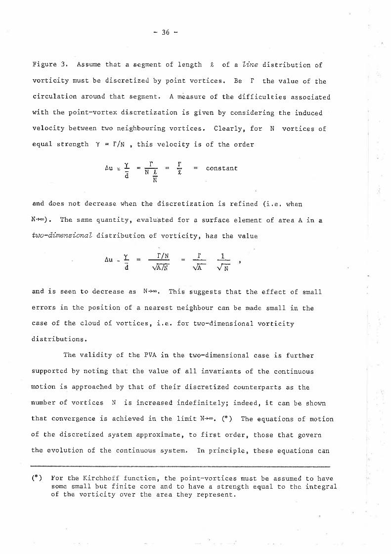
Figure 3. Assume that a segmenÈ of length 9" of. a Line distribution of

vorticity must be discretized by point vorEices. Be f the value of the

círculation around that segment. A màasure of the difficulties associated

with the point-vorÈex discretizaEion is given by considering Èhe induced

velocity between two neighbouring vortices. Clearly, for N vortices of

egual strength Y = f/N , this velociEy ís of the order

constant

ñ'

and does not decrease when the discretization is refined (i.e. when

N*) . The same quanÈity, evaluated for a surface elemenE of area A in a

two-dimensionaL distribution of vorticíty, has Èhe value

Âu-L r/Nd

and is seen to decrease as N+-. This suggests that the effect of small

errors in the posit.ion of a nearest neighbour can be made small in the

case of the cloud of vortices, í.e. for two-dimensional vorËicity

distributions.

The validity of the PVA in Èhe two-dimensional case is further

supported by noting that Èhe value of all invariants of the contínuous

motion is approached by that of Eheir díscretized counterparts as Ehe

nunrber of vortices N is increased indefinitely; indeed, it can be shown

thaÈ convergence is achieved in Èhe limit N-+-. (* ) The equations of motion

of the discretized system approximaÈe, to first order, Ëhose that govern

Ëhe evolution of Ëhe continuous sysEem. In principle, these equations can

(*) For the Kirchhoff function, the point-vortices must be assumed t,o havesome smaLl but finite core and Eo have a strength equal to the íntegralof the vorLicit.y over the area they represent.

Au=Id

T

N ,8,

f7

T1\Ã- \¡ì{\EÑ-

/A

Figure 3: Point Vortex Approximation for a line and asurface distribution of vorticity.

0123 Ja NG )C-(J)

b

u(

o

23

IoL

I)

II

{ bqE- U

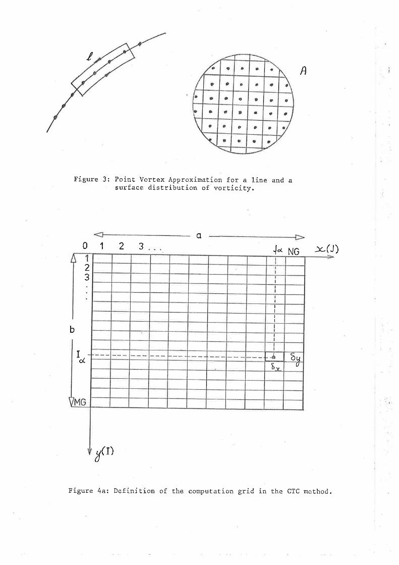
Figure 4a: Definition of the computation grid in the CTC merhod.

-37-

be solved exacEly; in pracLice, the accuracy of the computation may be

checked by monitoring the conservation of Èhe invariants.

These argumenËs seemed a justification to proceed r.¡ith the poinÈ-

vortex approximation, latgeLy in the spirit of an experiment. In artcloud

díscretizatLon" calculation, vortíces are not tracked exactly, and one

does not expect the phenomena determined by local flot¿ conditions to be

described faithfully. Integral expressíons - that is, expressions computed

over Ehe whole populatíon of vortices - are however compuÈed accurately, in

the limits indicated by the flow invariants. Flow features are determined

staÈistically, as resulting from several computations with varying initial

conditions. Each particular discretization can be regarded as one

reaLizatíon from a statistical ensemble. In this statistical interpretation,

it ís conjectured that an ensemble average over random discretizations

defines a solution of the continuous problem (NlíLínazzo of Saffman, L977).

A new vorËex-t,racing algorithm, Èhe centre-Eo-centre (CTC) method,

well suited to the cloud d:'-screÈization spirit, r¡üas developed and used in

à11 PVA calculations presented in this work. The remainder of this chapter

is dedicated to the presentaticn of the CTC ureÈhod.

TT.4 THE CENTRE-TO-CENTRE }ÍETHOD

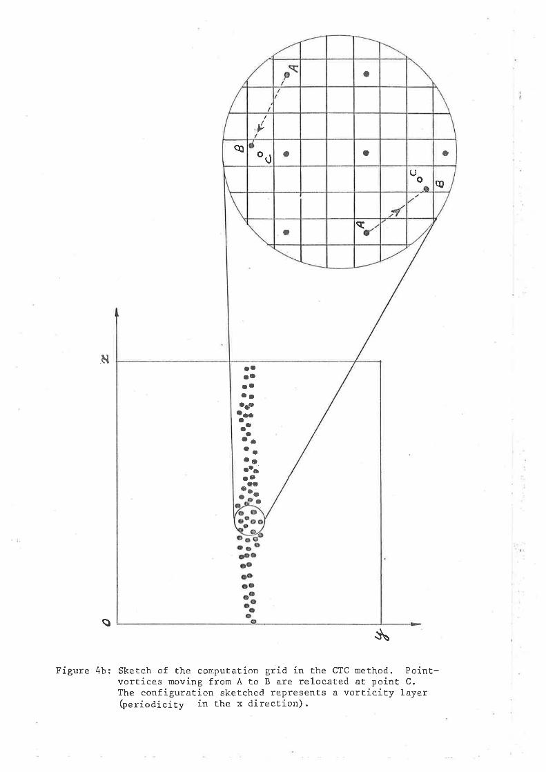
The motion of the vortices is followed over a fixed computation

grid, vrhich paves the interval of interesE with a large number of rectangular

ce1ls, as illustrated in Figures 4a & b. No a priorí attempÈ is made to

Erack the vortices exactly. AÈ all stages of the computation, the

coordinates of all vortices are deliberately ídentified with those of the

centre of the cell in which they happen to lie. Vortices move, therefore,

from cell-cenËre to cell-centre over the computation grid. This tracing

o

tca or.) o O

Uo a

,q

ooca

aÕ3

aa¡O¡OO¡odD

ooooaooO¡ooo¡Oaao

a

N

s$

Figure 4b: Sketch of the computation grid in the CTC urethod. Point-vortices moving from A to B are relocated at point C.The configuration sketched represents a vort.icity layer(periodicity in the x direcÈion).

-38-

algorithm is accordingly called the centre-to-centre (CTC) method, and

will be shown to possess properties that make it a valid alternative to

many vortex-!racing schemes reporEed in the literature.

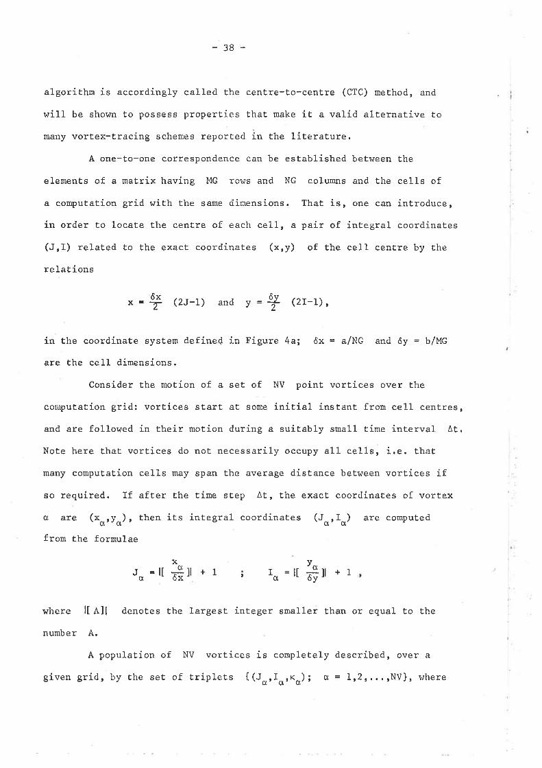
A one-to-one correspondence can be established between the

elements of a matrix having MG rows and NG columns and the cells of

a computation grid with the same dimensions. That is, one can introduce,

in order to locate the centre of each cell, a pair of integral coordinates

(JrI) related to the exact coordinates (xry) of the cell centre by the

relat ions

x= ôxT (2J-1) and y ôv2

(2r-1) ,

in the coordinate system defíned in Figure 4a; ôx = a/NG and ôy = b/MG

are the ce1l dimensions.

Consider the motion of a seË of NV point vortices over the

conrputaÈion grid: vorÈices start at some initial instant from cell cent,res,

and are followed in their motion during a suítably sma1l time interval At.

Note here that vortices do noÈ necessarily occupy all cel1s, i.e. that

many computat.ion ce1ls may span the average distance between vortices if

so required. If after the time step At, the exact coordinates of vortex

o are (xoryo), then its integral coordinates (J.,rIo) are computed

from the formulae

xJ = ll &0 I +1g

t ro =lt #1 + 1

where ll All denotes the largest inËeger smaller than or equal to Ehe

number A.

A populatíon of NV vortices is completely described, over a

given grid, by the set of triplets { (JclrIo,"o); o = L12r... rNV}, where

K0

39-

denotes the strength of vorEex cr . The initial flow configuration is

prescribed as the set of values { (J;, ri, r<l) ¡ q = L ,2, .. . ,NV} . The

cornputàd from the interaction law and Ëhevelocity of each vortex can be

new positions of the vortices

of motion.

determined by integration of the equat,ions

A few preliminary comments are warranted. The CTC method removes

the possíbílity of occurrence of high-induced velocíties by effectively

preventing vortices from approaching one another too closely. The cel1

dimensions act as a criËical approach distance: if two or more vortices

happen to lie within the same cell at Èhe end of a time step, they are

thereafter regarded as a single vortex, Èhe strength of which is the sum

of all indívidual vortices. The component vorËices remaín, however,

identifiable, since they retain Èheir labe1 ín the set of triplets

describing the configuraËions.

The introduction of integral coordinates significantly ímproves the

computational aspect of the summation algorithn. Distances between vortices

are necessarily integral multiples of ce11 dimensions; many operations can

be carried out using inÈeger arithmetic when evaluating the inÈeraction

sunmations. This is of particular interest on smaller compuÈers where

floating-point arithmetic operations are especially time-consuming. In

the special case rn¡here row-vort.ices are tracked, the hyperbolic and

circular functions appearing in the ttinfluence coefficientst' of the

interaction summations (see equat,ions [ 1.56] and [1.57]) can be tabulated

once and for all; the velocity of each vortex is then readily computed

from table rrlook-ups" and simple arithmetic operaËions. Adoption of this

technique substanÈially reduces the amount of computing time (by approxi-

mately one order of magnitude). VorÈex coordinates are integer numbers

-40-

r¿hich are easily paeked/unpacked for efficient, internal and external

storage. Again, this feaËure may be appealing when vrorking with machine

configuraËions where available memory'space is limited; it is even more

effecÈive when equi-strength vortices are employed, each configuration

requiring only the specification of NV pairs of coordinates

{(Jorla); cl = 112r,,. rNV} for its complete description.

The Èracing algorithm must, now be completed by the choice of a

numerical scheme for the integration of the equations of motion. Many

opEions are available; the choíce is however limited by pracEical

considerations of cost versus precision. The simplest and most. economical

scheme ís the one-step forward algorithm known as Eulerts method, which

relies on the first-Èerm of a Taylor series expansion. This method has

been used by many auEhors (nosenhead, 1931-; Kuwahara & Takami , L9733

Acton, L976). Higher-order schemes have also been employed, usually

belonging Ëo the family of Runge-KuËta formulae (Moore, Lg74 ; zaLosh,

L976); they are prohibitively expensive, however, when the number of

vortices becomes relaÈively large (a few hundred).

The properÈies of the CTC algorithm, coupled with the effects of

the integration scheme, have been sysÈematically investigated by comparing

computed flows with an exacE reference flow, the disk of uniform vorticity;

this investigaEion is described in detaíl in Sections II.5 & II.6.

II.5 EFFECTS OF INTEGRATION PROCEDURE TIME STEP AND CELL SIZE IN THE

CTC METHOD

The purpose of this section is to present the first series of tests

carried out to quantify the performance and Ëo undersËand the fundamenÈa1

properties of Èhe CTC meÈhod. If the method is applied to compute the

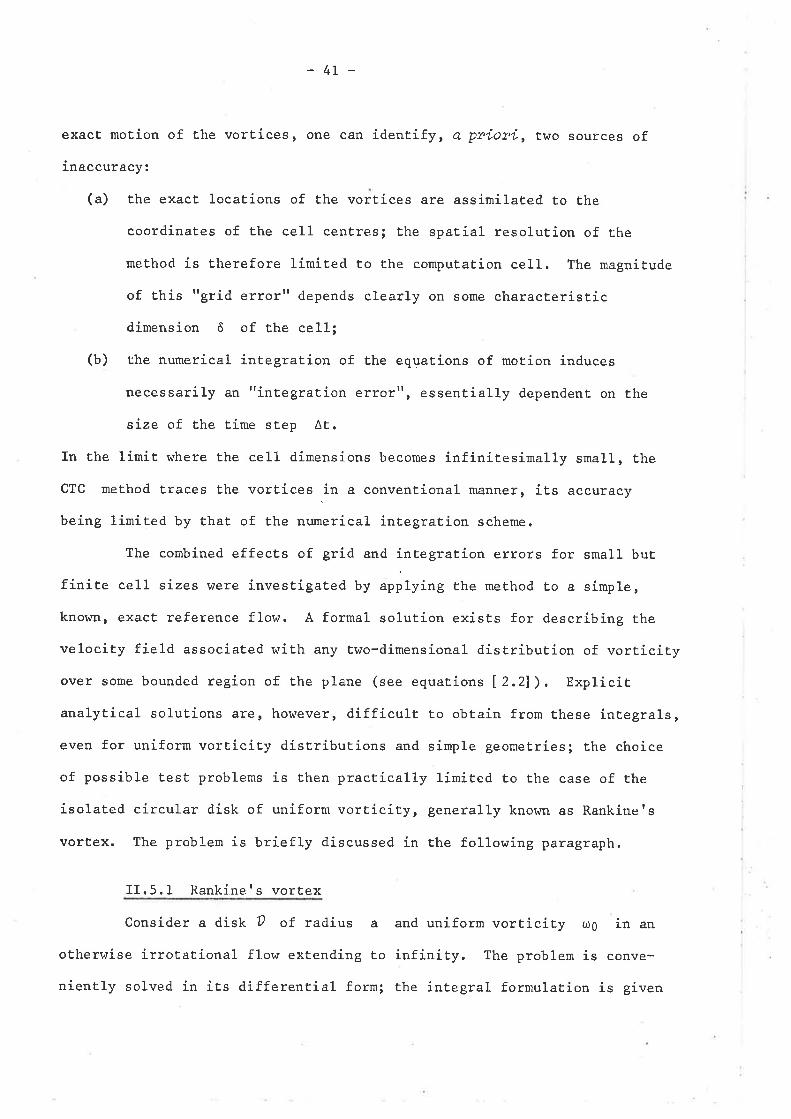
-4L-

exacË motion of the vorEices, one can identífy, a prioní, two sources of

inaccuracy:

(a) the exact locations of the vortices are assimilated to the

coordinates of Êhe cell centres; the spaËial resolution of the

method is Eherefore limíted to the computation cel1. The magnitude

of this ttgrid errortt depends clearly on some characteristic

dimension ô of the cell;

(b) the numerical integration of the equations of moËion induces

necessarily an ttintegration errortt, essentially dependent on the

size of the time st,ep ^t.

In the limit where the celI dimensions becomes infinitesimally smal1, the

CTC method traces the vortices -in a convenÈional manner, its accuracy

being limited by that of the numerical integration scheme.

The combined effects of grid and integration errors for small but

finite cell sizes r¡üere invest,igaEed by rnpfrirrg t,he method to a simple,

known, exact reference flow. A formal solution exists for describing the

velocity field associated with any two-dimensional distribution of vorticity

over some bounded region of the plane (see equations 12.21>. Explicit

analytical solutions are, however, difficult to obtain from these int,egrals,

even for uniform vorticity distributions and simple geometries; the choice

of possible test, problems is Lhen practically limited to the case of the

isolated circular disk of uniform vorticity, generally known as Rankinefs

vortex. The problem is briefly discussed in the following paragraph.

II.5.1 Ranki,ners vortex

Consider a disk ? of radius a and uniform vorticity ûr0 in an

oËherwise irrotational flow extending to infinity. The problem is conve-

niently solved in its differential form; the íntegral formulation is given

-42-

in Appendix B.

The stream function rþ must. satisfy the

v2V=-, innid" D

v2ú= o outside D

The circular synrnetry is preserved rvhen ûJ and

radial distance only; steady motíon is possible if

funcËion of rir. For üJ constant(= ulO), one has

and

rre A Lo9r+Be

¿2,ltã77

and [ 2.41

fl..!9ü=o ourside Dotz r or

The general integral of this equation is rl,(r) = A log r + B; a particular

solution of Ehe nonhomogeneous forms is ú(r) = - uor2/4. Therefore, the

internal and exÈernal solutions are, respectively,

üi=Ailogr*Bi-usr2/4

+ lgV+oô=oin 0rdr

equations

Í 2.31

tl, are functions of the

ís an arbitraryu)

[2.s]

e

The requiremenÈs that rl be finite at r = O and thaÈ rp and

continuous at the disk boundary lead to

dúdr be

úi(r)=+ G2-'2)

and I 2.61

1og r,

+loga

ü"(r) = - 'Ët

Be

where Èhe addítive constanE has been omitted. The velocity potential

-43-

outside Ehe disk is found to be

0. (x'l) + r.an-l(y,x¡

úe is a mulËiple-valued function with cyclic consLant l' = 2t

The velocity fíetd is derived from

+ =r^2

l2 .71

t 2.81

I 2.el

(')0.

ur 1 3s.r â0 e3tðru =-

2

and is found to be

p(r)

uu (r) ? r within D

uu (r)

"3P--PT ouËside0.

p (r) y2

t

ouÈside 0

The disk roÈates about its axis as a rigid body with angular velocity

Q = uO/2, corresponding Eo a period of rotation T = 4r/uO,

For the sake of completeness, let us mention that Ehe pressure

field is determined from Eulerrs equation of motion inside 0 and

Bernoullits relaËion outside 0. One obtains:

20 gl.

dr giving p (r)2

? e + +p(o) inside Du !

pt ,

Continuity of the pressure field at r = a leads to the results

p (r)

-21-' ínside DZa2

P

P

Iæa

( T uJoa22 )

and

t2r

æ&.212

outside D

[ 2.10]

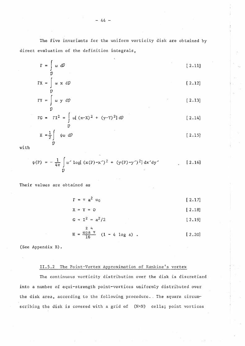
-44-

The five invariants for the uniform vorticity aist are obtained by

dírect evaluation of the definition inEegrals,

I2.LLl

I2,L2l

[ 2.13]

T

d0

dD

Ð

x

v

=f.,D

=I,D

=f,D

TX

TY

IG= 1I2= r.¡r[ (x-x)2 + (v-Y)21aO

þu d0

1

ID

,JJ (P) 4r u:' 1og[ (x(P) -x')2 + (v(p) -y)zfdx'dy'

Their values are obtained as

I=na2uo

X=Y=O

G=L2=^2/224

JD

| 2.r41

[ 2.ls]

T 2 ,L6I

I 2,2oj

| 2,L71

[ 2.18]

| 2.rel

" =+lD

wirh

]l= (1-41oga)

(See Appendix B).

II.5.2 ttre Point-Vortex Approximation of Rankiners vortex

The continuous vorticity distribuEion over the dísk is discretized

into a number of equi-strength point-vortices uníformly distributed over

the disk area, according to the following procedure.. The square circum-

scribing the disk is covered v¡ith a gríd of (NxN) cells; poinÈ vortices

-45-

are then placed at the centres of all ce1ls which belong to the interior

of the disk. The number of vortices retaíned is approximaËely equal to

NV = 0.8 N2. This discretization procedure is clearly synrnetrical and

ensures that the resulting point-vortex disÈribution approaches uniformity,

for NV large. Boundary effect,s, however, cannot be ful1y eliminated and

a::e reflected in the values of the invariants G and II (I, X and Y achieve

their Èheoretical value) (see Table 2),

The smallest distance between adjacent vortices is A = 2a/N. The

motion is usually computed over a fine mesh computation grid of cel1 size ô.

It is convenient to select the ratio Â/ô = N6 as an odd integer, in order

to keep the initial configuration unaltered by the redefínition of the

grid (Figure 5).

The influence of the two basic parameËers ô (cell size) and ^E

(tíme step) was investigated on the basis of a comprehensive number of

computer runs. For reasons previously exposed (see secËion II.3), it

seemed crucial to evaluate the invariants of the florv, particularly Ehe

Hamiltonian or Kirchhoff function of the system: it appears importanE to

ensure thaE in its final state, the system possesses the same Eotal energy

as that of its initial configuraEion. If this energy were not conserved,

the mechanisms responsible for the loss of invariance had to be identified

and the rnagniÈude of their effects appreciated. The behaviour of the

Ëhree other invariants X, Y and G was also considered. In all computations,

covering a wide range of values for cell size and Eime step, Èhe centre of

vortícity (X, Y) of the cloud was found to remain fixed with a high degree

of accuracy. Results presented concern almost exclusively the behaviour of

the Kirchhoff function H of the system. The behaviour of Èhe radius of

gyrati.on I = vF \,ras hov/ever monitored in order to confirm the conclusions

drarn¡n from the function H; in all cases, conclusions draum independently

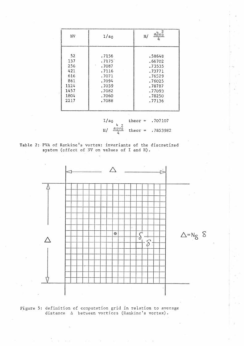
NV t/ ao

î/ ao

u/t+2

e 0ûr04

theor =

theor =

.707 ro7

,7853982

Table 2: PVA of Rankiners vortex: invariants of the discretizedsystem (effect of NV on values of I and H).

A

A

F.igure 5: definition of computation grid in relation to averagedistance A between vortices (Rankiners vortex).

A,=N6 E

Ttl

5213725642L6t6861

TI24L457180422t7

.7L56

.7175

.7087

.7IL6

.707r

.7094

.7039

.7082

.7060

.7088

.58648

.66702

.7 3535

.737 7 L

.7 6529

.7 6025

.7 87 87

.77093

.78250

.77136

o

1

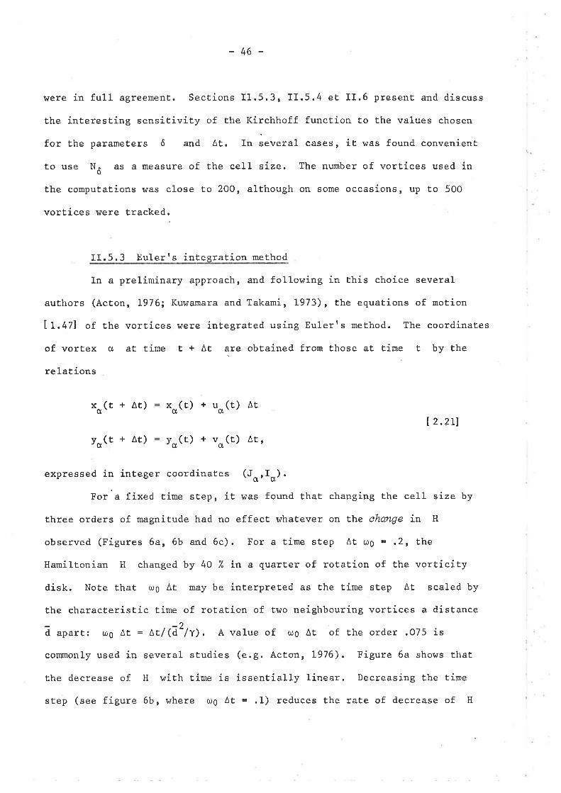
-46-

tvere in full agreement. Sections II.5.3, II.5.4 et II.6 present and discuss

the interesting sensitivity of the Kirchhoff function to the values chosen

for the parameters 6 and ^t.

In s"v"ral cases, it was found conveni-ent

to use Nô as a measure of the ceIl size. The number of vortices used in

the computations was close Èo 20O, although on some occasions, up to 5OO

vortices were tracked.

II.5.3 Eulerrs integration method

In a preliminary approach, and following in this choice several

auÈhors (Acton, I976; Kuwamara and Takami, L973), Èhe equations of motion

Lt,t+l) of the vortices were integrated using Eulerrs method. The coordinates

of vorEex cl at time t + At are obtained from those at Ëime t by the

relations

xo(t + ar) o(r) + Ë

^r=x

Í 2.2r1

yo(t + At) +v ( E Âttct

expressed in integer coordinates (JorIq).

For a fixed time step, it was found that changing the cell size by

three orders of magnitude had no effect rn'hatever on the chartge ín H

observed (Figures 6a, 6b and 6c). For a time step At trlg = ,2, the

HamilÈonian lI changed by 40 7. ín a quarter of rotation of the vorticity

disk. Note that urg At may be inEerpreted as the time step At scaled by

the characteristic time of rotation of Ërnro neighbouring vortices a distance

ã .p"tt: o0 At = At/ (Ã2/Ð. A value of urg At of the order .075 is

commonly used in several studíes (e.g. Acton, L976), Figure 6a shows that

Ehe decrease of H with time is issentially linear. Decreasing the tirne

step (see figure 6b, where o9 At =.1) reduces the rate of decrease of H

u ( )o

= yo(t) )

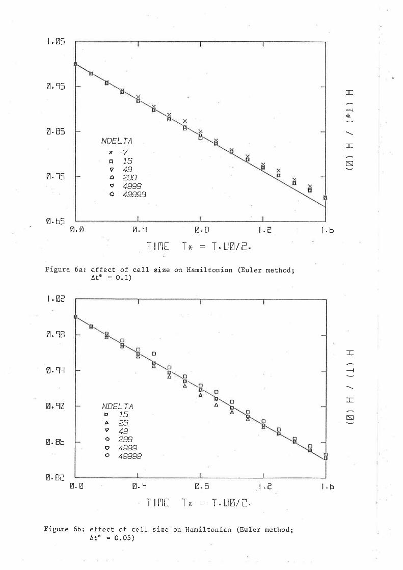
l.Ø5

Ø, q5

ø.85

ø.15

Ø.b5

=--1*

=ñ

Ø.Ø Ø. I Ø.8

Tlnt fx = I"AØ/e.

r.e l.b

Figure 6a: effect of cel1 size on HamilEonian (Euler method;AE* = O.1)

Ø¿

Ø.98

ø.qr

ø.1Ø

Ø. Bb

Ø.Beø.Ø Ø.r Ø.8 r.e

Tlnt T* = T.tìØ/¿"

Figure 6b: effecE of cell size on Hamiltonian (Euler method;Ar* = O.05)

I

--{

I

N

NDELTAx7tr15e49ô 299v 4999ó' 49999

A

ANDELTAÞ15ô25v49ô 299e 4999o 49999

b

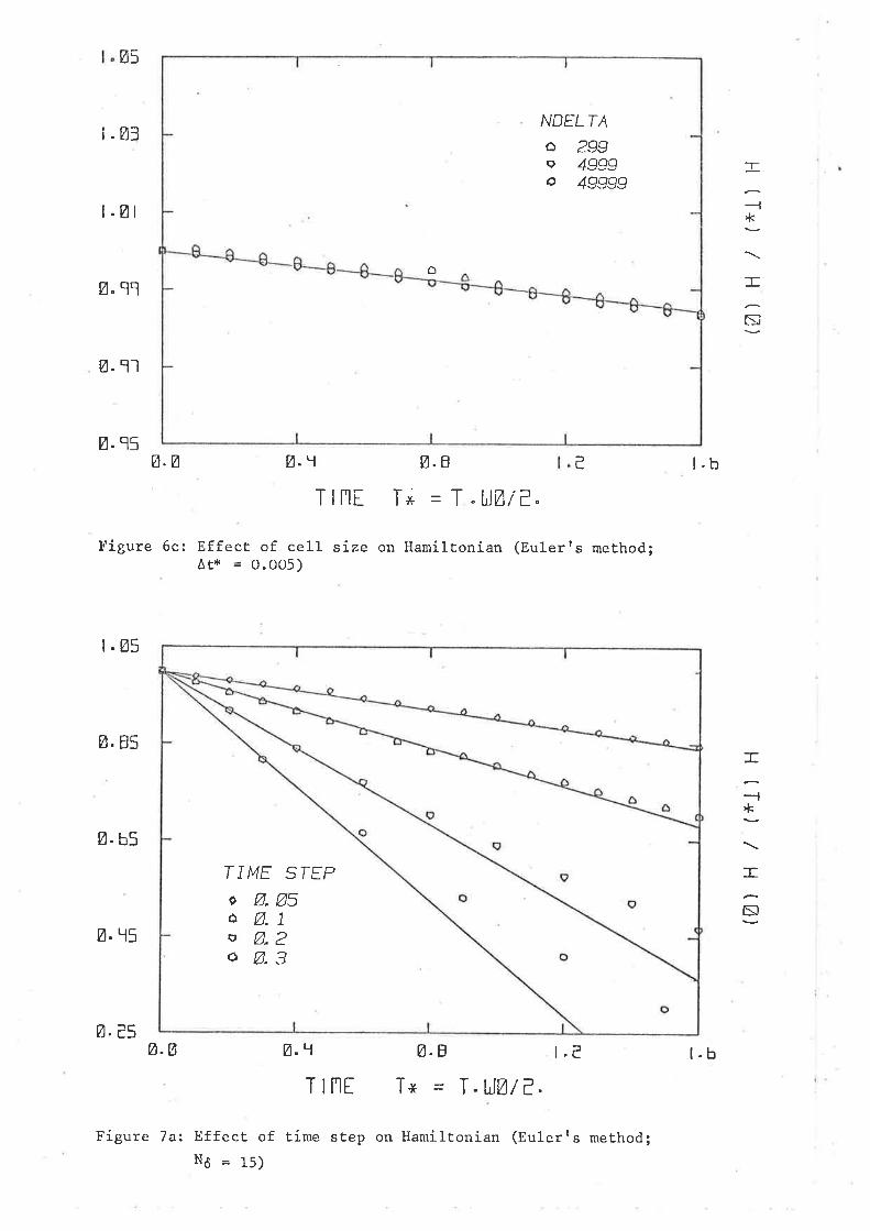
Ø5

i -Ø3

t.øt

Ø. qq

Ø.11

E.q5

-r

-l'k

:tr

ñ

Ø.Ø Ø-T

ø.1

Ttn[

Ø.8

Tlni Tx -T"UØi?"e l.b

Figure 6c: Effect of cell size on Hamiltonian (Eulerrs method;

^t* = 0.005)

r.Ø5

Ø. 85

Ø.b5

Ø.T5

Ø.¿5Ø.Ct ø.8 r.¿

Tx T.UØ/?.

Figure 7a: EffecE of time step on Hamiltonian (Eulerrs method¡Nô = 15)

=

-t*

:tr

N

ô

NDELTA

ô 299e 4999o 49999

TIME STEPo Ø.Ø5ô Ø. 1

o Ø,2o Ø.3

l.b

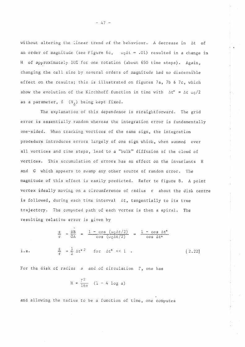
-47

without altering lhe linear trend of the behaviour. A decrease in At of

an order of magnitude (see Figure 6c, r.ogAt = .01) resulted in a change in

H of approximaÈely LO7" for one rotation (about 650 time steps). Again,

changing the cell size by several orders of magnitude had no discernible

effect on the results; this is illustrated on figures 7a, 7b & 7c, which

show the evolution of the Kirchhoff function in time with Atx = Lt uo/2

as a parameter, ô (Nô) being kept fixed.

The explanation of this dependence is straightforward. The grid

error is essentially random whereas the integration error is fundamentally

one-sided. Llhen tracking vortiees of the same sign, the integration

procedure introduces errors largely of one sign which, when summed over

all vortices and time steps, lead to a "bulk" diffusion of the cloud of

vorEices, This accumulation of errors has an effect on the invariants H

and G which appears to swamp any other source of random error. The

magnitude of thís effect is easily predicted. Refer to figure B. A point

vortex ideally moving on a circumference of radius r about Èhe disk centre

is followed, during each time interval Àt, tangentially to iEs true

trajectory, The computed path of each vortex is Ehen a spiral. The

resultíng relative error is given by

1

e

r

BB

õA1- cos (rrr¡AE/2)

-crs rcroãTÐ

1 - coe At*cos AÈx

I^t*

2 for At* << 1I¡ê. )

For Ehe disk of radius a and of circulation f, one has

[ 2.221

(I-41oga)r2u-¡rr-._-I blr

and allowing the radius to be a function of time, one computes

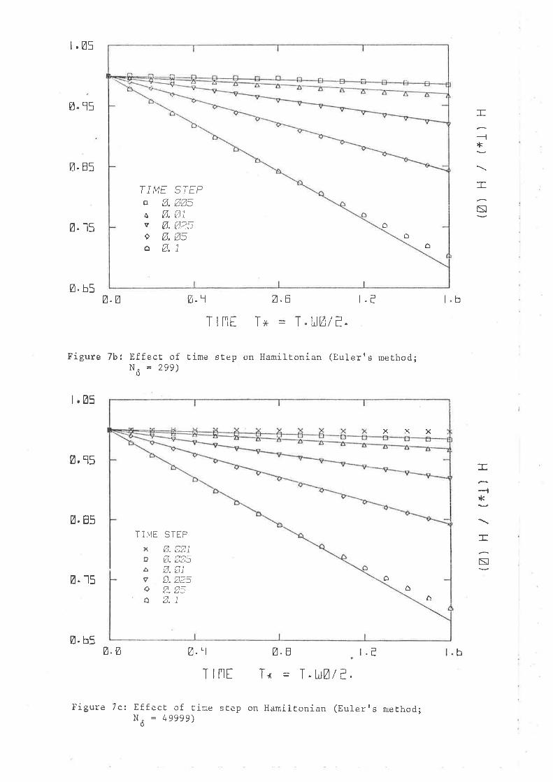
ôô

ô

TIMEsØ.öØ.vØ.oØ.ôØ.

STEPØØ5Ø1

Ø25Ø51

l.Ø5

Ø.15

Ø.85

Ø.15

Ø.b5

ø.15

Ø.ø

r----t,k

=ñ

Ø.1 Ø. B

Tlnt Tx = r "uØi-"

Figure 7b: Effect of tíme sÈep on Hamiltonian (Eulerrs method;NO = 299)

l.ø5

ø. q5

ø. Ê5

Ï]ME STÍPx Ø- ãØio Ø. DØ5ô Ø.Ø1e Ø. Ø25o Ø.Ø5o Ø. 1

ø.b5ø.Ø Ø.8 r.¿

T+ = T.UØ/?.

t.e b

:tr

*

:tr

ñ

ø.1

T rnt

l'igure 7c: Ef f ecÈ of time st.ep on Hamiltonian (Eulerts method;NU = 49999)

XXX

ôò

A

b

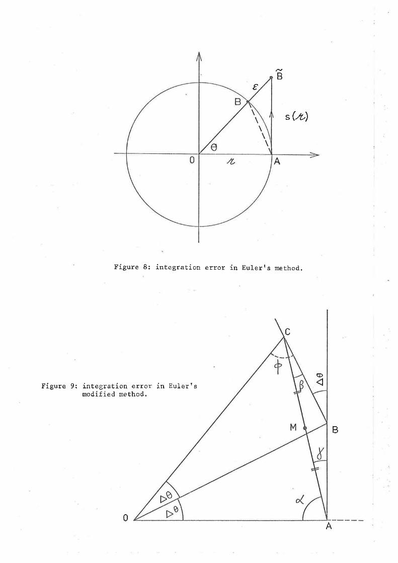
B€

s (.?')

Figure 8: integration error in Eulerrs method.

A

C

(D

Figure 9: integration error in Eulertsmodified method.

B

0A

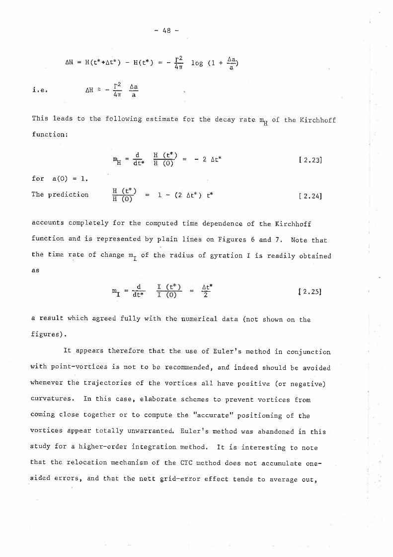
l.e AH:

This leads to the

funct íon ¡

-48-

aH=H(tx+At*) -H(Ë*) -#1oe(r.þ

following estimate for the decay rate nH of the Kirchhoff

¡2 aaña

for a(O) = 1.

The prediction 1 (2 At* ) t* I 2.241

accounËs completely for the computed time dependence of the Kirchhoff

function and is represented by plain línes on Figures 6 and 7. Note tha¡

the Èime rate of change m, of the radius of gyration I is readily obtained

as

dh dt*E__(c-)H (o) -21|.*

^t*T

I 2.231

t 2.2s1tr dãF

a result whích agreed fully with the numerical data (not shown on the

figures).

It appears therefore that the use of Eulerfs method in conjunction

with point-vorËices is not to be recommended, and indeed should be avoided

whenever the trajectories of the vortices all have positive (or negatíve)

curvaÈures. In this case, elaborate schemes to prevent vortices from

comíng close together or to compute therraccurate, positioning of Èhe

vortices aPpear totally unwarranted. Eulerrs method r^¡as abandoned in this

study for a higher-order integration meÈhod. It is interesting to note

that the relocation mechanism of the CTC method does not accumulate one-

sided errors, and that the nett grid-error effect tends to average ou¡,

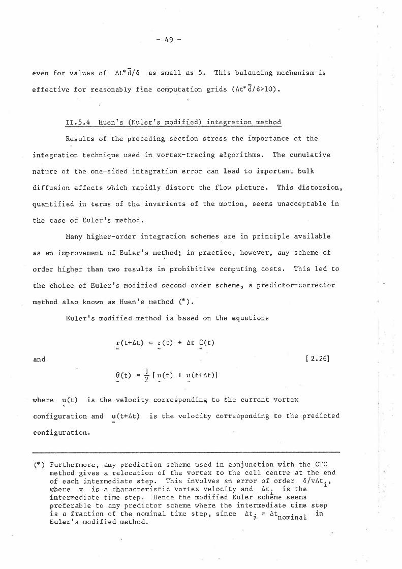
even for values of ^t*ã/ô

as

effective for reasonably fine

-49-

small as 5. This balancing mechanism is

compuration gríds (AtxA/ô>10).

II.5.4 Huenrs (Eulerrs modified) integration method

ResulÈs of the preceding section stress the importance of the

integration technique used in vortex-tracing algorithms. The cumulaÈive

nature of the one-sided íntegration error can lead to importanl- bulk

diffusion effecÈs which rapidly distort Ëhe flow picture. This distorsion,

quantified in terms of the invariants of the motion, seems unacceptable in

Èhe case of Eulerrs method.

Many higher-order integration schemes are in prínciple available

as an improvement of Eulerrs method¡ in practice, hovrever¡ any scheme of

order higher than two results in prohibitive computing costs. This led to

the choíce of Eulerts modified second-order scheme, a predictor-correcËcr

method also known as Huenrs method (*).

Eulerrs modified method is based on the equations

r (t+At) r(t) + Ar û(t)

and Í 2.261

where u(t) is the velocity

confíguration and u(t+At)

confi gurat ion.

û(t) = !, tu(r) + u(r+¡r)l

correèponding to the current vortex

is the velocity corresponding Èo the predicted

(*) Furthermore, any prediction scheme used in conjunction vrith the CTC

method gives a relocation of the vortex to the cell centre at the endof each inÈermediaEe step. This involves an error of order ô/vAt;rwhere v is a characteristic vortex velocity and At., is theintermediate time step. Hence the modified Euler schËme seemspreferable to any predictor scheme where the intermediate time stepis a f raction of Ehe nomínal time step, since At., = AÈ---., -1 inEulerrs modified method

- 1 nomrnar

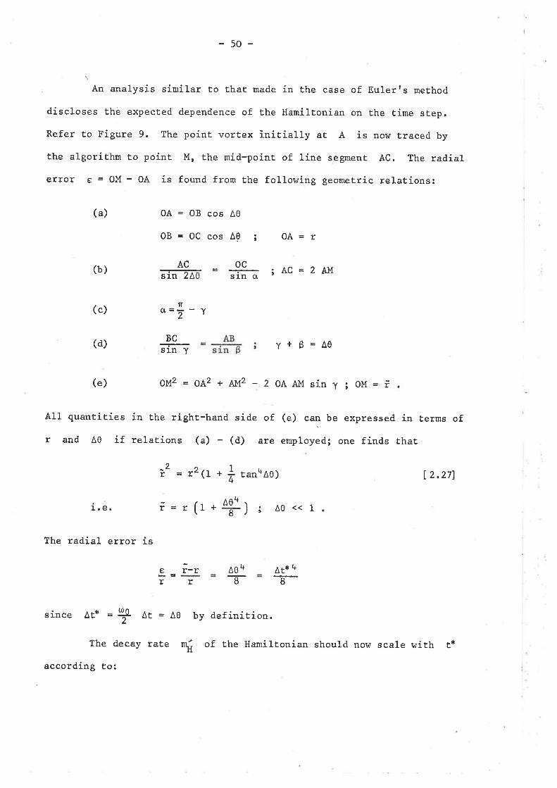
-50-

*Arr.rrrlysis similar to that made in Ëhe case of Eulerrs method

díscloses the expected dependence of the Haniltonian on the time step.

Refer to Figure 9. The point vortex initially at A is nor¿ Ëraced by

the algorithm to point M, the mid-point of line segment Ac. The radial

error e = oM - oA is found from the followíng geometric relations:

(a) 0A = OB cos À0

OB=OCcosA0 ; OA=r

(b) Acãfn7-g" - #* ;AC=2AM

(c) 1To=z - T

(d)

1.ê

The radial error is

Y+ß=40

); Ao<<1

^t* 4

8

BC

s]-n Y

t

i = r (t + Ae48

(e) oM2 = oA2 + 4¡12 - 2 oA At"I sin y ¡ oM = i

All quantíties in the ríght-hand side of (e) can be expressed in terms of

r and A0 if relations (a) (d) are employed; one finds rhar

2r = rZ(L +T1 ran4^o ) | 2.271

-tr

er

A04I

since At* + aE = ao by definition.

The decay rate r" of the Hamiltonian should now scale with t:r'

accordíng to:

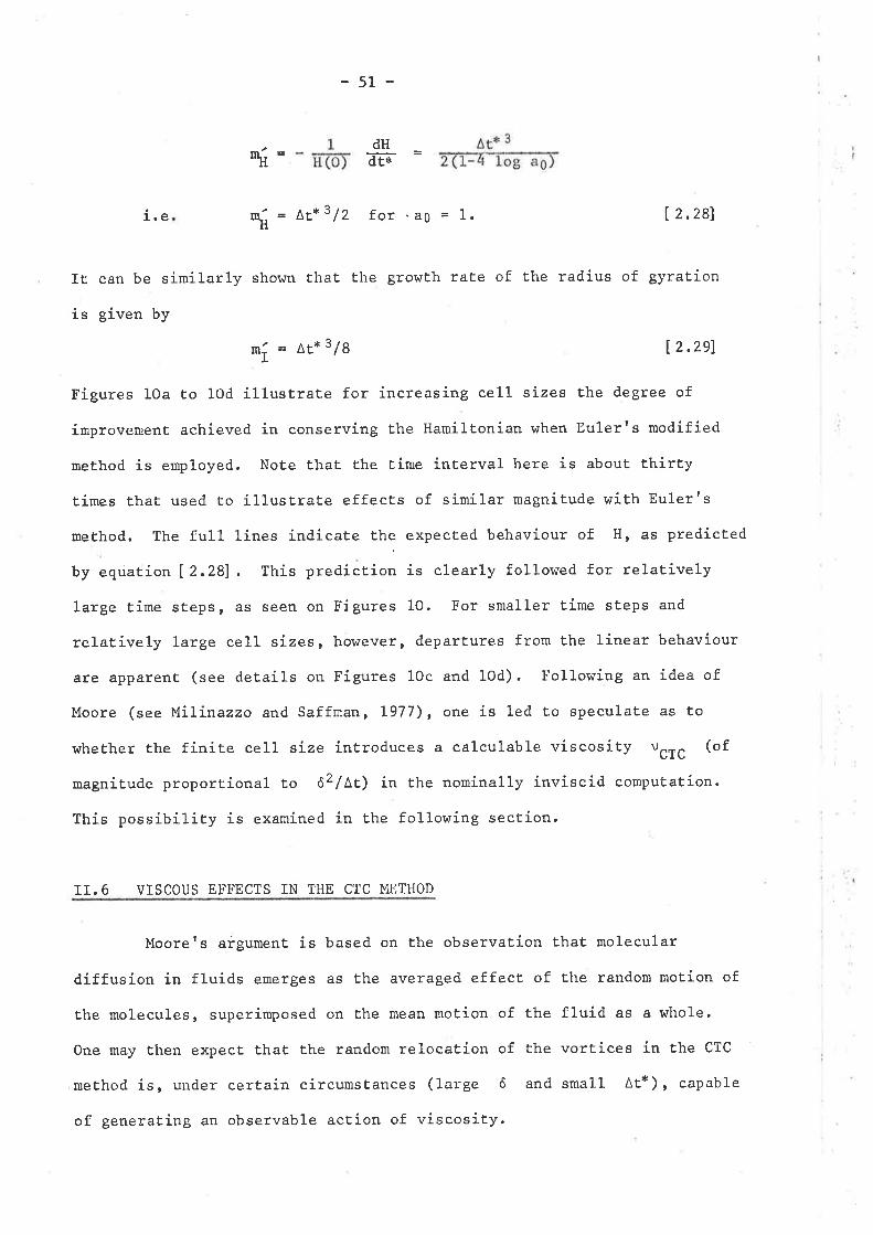
-51 -

d

\

dHãr*

1.e = Lt*3/2 for .ao = 1, I 2.28)

It can be sirnilarly shown that Ehe growÈh raËe of the radius of gyraÈion

is given by

mí = lr" 3/8 12.291

Figures lOa to lOd illustraÈe for increasing cell sizes the degree of

improvement achieved in conserving the Hamiltonian when Eulerrs modified

method is enrployed. Note thaL the Èime interval here is about thirty

times thaE used to illustraEe effects of similar magnitude v¡ith Eulerrs

method. The ful1 lines indicate Ehe expected behaviour of H, as predicted

by equation [ 2.281 . This predicÈion is clearly followed for relatively

large time steps, as seen on Figures 10. For smaller time sÈeps and

relatively large ce11 sizes, however, deparEures from the linear behaviour

are apparent (see details on Figures 10c and lod). Following an idea of

Moore (see MiliÍtazzo and Saffman, 1977), one is led to speculat,e as to

whether the finite cell size introduces a calculable viscosity uCtC (of

magnitude proportional to ô2/At) in the nominally inviscid computation.

This possibility is examined in the following section.

II.6 VISCOUS EFFECTS IN THE CTC METHOD

Moorets aigument is based on the observation Èhat molecular

diffusion in fluids emerges as the averaged effect of the random motion of

the molecules, superimposed on Ehe mean motion of the fluid as a who1e.

One may then expect, that the random relocation of the vortices in the CTC

method is, uncler certain circumsÈances (large ô and small At*), capable

of generating an observable action of viscosity.

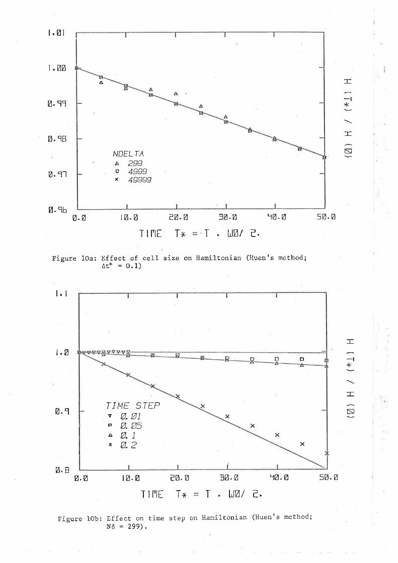
A

NDELTAA 299o 4999x 4gggg

l.Øl

t -Øø

Ø.qÎ

ø.18

ø.11

ø. qbØ.ø JØ.ø

I UØt E.

T,Ø. ø 5Ø.ø

Figure l0a: Effect of cel1 size on Hamiltonian (Huenrs method;At* = O.1)

I,l

t.ø

ø.q

ø Bø.ø tø-ø ¿ø-ø

Tlnt Tx

3ø.ø T,ø.Ø

uØ/ E.

Figure lOb: EffecÈ on time step on Hamiltonian (Huenrs method;

=

-1*

:tr

S

tø.Ø eØ-ø

Tlnt Tx

I

-t,k

=ñ

T

o

xx

xx

eØ1Ø51

2

TEPTIMEvfl.ÞØ.AØ.xfr.

Nô = 299).

5Ø.ø

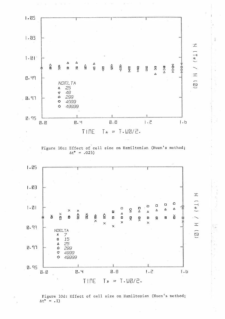
q

(T . = 4lV!poqlaur s¡uang) ueruofTrt¡Ieg uo azrs TTac l:o lcal:fã :POT arn8TJ

"¿/Øn" L = xl lU l1

¿'lg'øh'øø'Ø

(çZO. = *tVÍpoqfau s¡ueng) ueruolT-rueH uo azrs TTaJ ]o lcaJl:Í :cA1 a:n31t

"¿iØn"!, = *1 lUll¿'l8'Zl-r'Ø

ñ

:t

+l-

=

5h'Ø

Lb'ø

irb'ø

rØ' I

Eø. I

5Ø' I

5b"ø

Lb'Ø

bh'Ø

tø' !

EØ.I

q

[:¡

T

+t--

:I

xxxx .. x XqEusðð:G'gti FH€gq -vev-E eev'åÜoexxooou

6666Þ o666' ô662 oSZeçfoLx

v1-r:oN

6v

E

vtvg

v

V

IvI

ÒÒbbv6667

66¿6F9Z

VJ11

EEgv

ËÊå

YI Ã

vçr

oô(2

Av

ON

sr¿'I

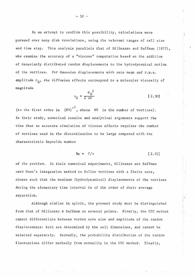
-52'

In an atEempt to confirm this possibility, calculatíons were

pursued over many disk revolut.ions, usí-ng the relevant ranges of cell size

and t,ime step. This analysis paralleis that of ltí!ínazzo and Saffman (1977),

who examine the accuracy of attviscous" computation based on the addition

of Gaussianly distributed random displacements to the hydrodynamical motion

of the vortices. For Gaussian displacements ¡,sith zero mean and r.m.s.

amplitude oar the diffusion effecEs correspond to a molecular viscosity of

magnitudeÇc2

v re [ 2.30]

(to the first order in (NV)-Ì, where NV is the number of vortices).

In their study, numerical results and analytical arguments support the

view that an accurate simulation of viscous effecÈs requires the number

of vortices used in the discretization to be large compared with the

characteristic Reynolds number

Re = I/v [2.31]

of the problem. Ir'r their numerical experimenÈs, Milinazzo and Saffman

used Huents integration method to follow vortices with a finite core,

chosen such that the maximum (hydrodynamical) displacements of the vortices

during the elementary time interval is of the order of their average

separation.

Although similar ín spirit, the present study must be distinguished

from that of Milinazzo & Saffman on several points. First1y, Ehe CTC method

cannot differenËiate between vortex core size and amplitude of the random

displaeemenËs: both are determined by the ce11 dimensions, and cannot be

selected separately. Secondly, Èhe probability distribution of the random

flucËuations differ markedly from normality in the CTC method. Finally,

G

-53-

the existence of a random motion is subordinate to that of the hydrodynamical

moÈion pure diffusion effects cannot be directly rnodelledby Èhe CTC method.

I^lith these restrictions in mind, one can estimate Ehe values of an

equivalent core size and r.m.s. amplitude as follows. The square cell of

diurension ô is assimilated to a circular core of radius o = ð/lñ'. The

actual probability distribution of the relocation displacements is approxi-

mated by a uniform dístribution over the cell, yielding a mean square value

ql27 =

The

ucrc ô2TÑ Í 2,32)

The validity of this prediction may be tesËed by comparing the outcome of

the numerícal computations with the analytical soluLíon for the decay of a

uniform vorticity disk in a viscous fluid. It is possible to predict the

change with time of the Hamiltonian resulting purely from díffusion at Èhe

boundary of the disk; comparison with the behaviour of H in Ëhe numerical

computaEions allows to infer the actual value of the viscosity in the CTC

method and a check on expression [ 2.321. Before presenËing the results of

these calculations, it is necessary to consider Lhe problem of the uniform

disk of vorticity in a viscous fluid and several related expressions; this

is Èhe object of Sections II.6.1 and IL6,2,

II.6.1 Viscous deeay of a vorticity disk

Consider a vorticity disk of radius a and uniform vorticity u)o

and its motion in an otherwise inítia1ly irrotational viscous fluid

6

r (*2*y2) "2dxdy=3.6

rðô-z-T

calculated viscosity in the CTC method is Eherefore

-54-

extending to ínfinity. Viscous actíon at the disk boundary tends to smooth

out rhe step discontinuity in the vorticity distribution, Ieading to Ehe

spreading of the rotational region of the flow by a process of gradient

diffus ion.

In all generaliËy, the thro-dimensional vorticity distribution in a

viscous, incompressible fluid is governed by the scalar equaËion

tir=vv2t¡ [ 2.33]

- âv if : v ís Ëhe kinematic víscosity of the fluid. rn polarkTherer=ã;-ãy

coordinates (rr0), the above equatíon is rewritEen

ðr¡àË

âr¡l to âr¡r

1U-1--=rdr r du!t

r!r

t ('# )a L ð2u | 2.341

l2,3sl

12.361

v +a t x2 ao2

whereâu

rrl(r r 0)d

âr(ru6 ) - ão-

o(r(a

a<r<o

for all t>o

l

In view of the azimutal symmetry of Èhe problem of the disk, one needs only

consider functions which do not depend on 0 ; furthermore, it is clear that

the velocity fietd has no radial component (t, = o). l{ith these simplifi-

cations, the differential equations of the problem reduce to

âr¡E

v à âorã¡ ('ãl ,x

a Í 2,37)E (ru)

where u has been wriEten for u0. The boundary and inítial condiEions to

be satisf ied by t¡(r, t) are the f ollowing:

IûJ =- t

1imr->æ

ur(rro) = ûJo

o(rro) = o

o(r, t) = o

[ 2.38]

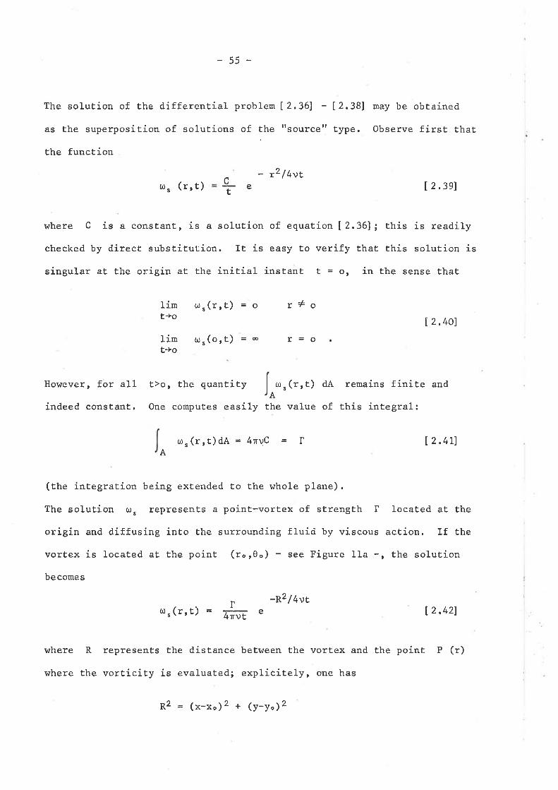
-55-

The solution of Èhe differenEial problem Í2,361 - [2.38]

as Èhe superposiEion of soluËions of the "source" type.

Ëhe funcÈion

may be obtained

Observe firsE that

[ 2.40]

- r2/4vtû) s

(r, t) e I 2 ,3el

where C is a consÈant, is a solution of equation 12.361; this is readily

checked by direcE substitution. IE is easy Èo verify that this solution is

singular at the origin at the initial instanË t = o, ir the sense ËhaE

ct

limt->o

limt'>o

=æ

t=to

r=o

t^r, (r, t) =o

t^l .(ort)

However, for all

indeed constant.

It)o ¡ the quantity I rrr . (r, t) dA remains f inite and

)¡One computes easily the value of this integral:

o. (r , t) dA = nvC r | 2 .4LlA

(the integration being extended to the r¿hole plane).

The soluÈion o. represents a point-vortex of sËrengEh I located at the

origin and diffusing into Èhe surrounding fluid by viscous action. If the

vortex is located aE the point (ror0o) - see Figure lla -, the solution

becomes

r,r.(r,r) = ?*E "-t2/4vr f2.421

where R represents the disLance between the vortex and the point P (r)

where the vorticity is evaluated; expliciÈely, one has

¡2=(x-xo)2*(y-y")2

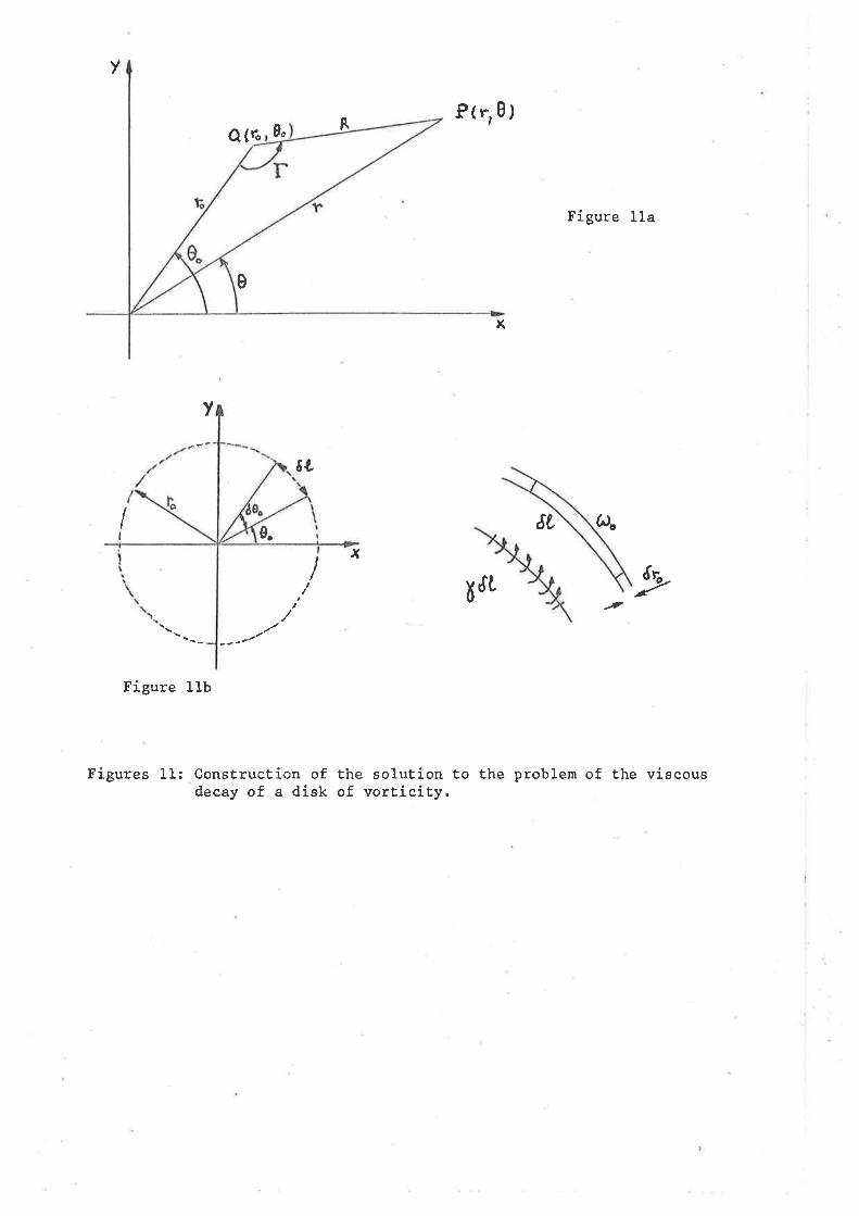
Y

RPtr,0¡

Q (ro 0o

Figure lla

0

x

v

II

6L

8L (^)t0n

xII IUûI,

-?

Figure 1lb

Figures 11: Construction of the solution to the problem of the viscousdecay of a disk of vortieity.

-56-

or R2=12+l-o2-Ztxo cos (e-0") f2,431

Consider nohr a continuous line-distríbution of circulaËion, defined

such that Ëhe amount of circulation "carried" by a line-element ôL has

the value 6¡ = yô0. Assume in addition that this line of circulation is

a circumference of radius Eo centered at the origin ; clearly then

ô!, = rod0. The viscous diffusion of a uniform "vorticity ringil is described

by the function

(r, t) ur. (r r t) dC

2r - R2/ 4vE

=fc

ü) c

Yfo4nvt

YroZ:rvt

f, e d0o

'(r2+ro2)/tvt 2r rro cod Le/2vt1.e. u) (r, t)

ce e

0

in terms of the solution

(see l^Iatson, 1922, 3.7).

d0" 12.441

Io of the modified

One rewrites the

The integral may be expressed

Bessel equat,ion of. order zexo

ríng solution under the form

ü) (r, t) e(r2+ro2) / +vt

(\xo2vtc

Io ftsom Í 2.4s1)

Note that the circulaEion per uniË length Y may be relaÈed Eo the local

value of the vorticíty oo as folloras. Consider the ring of circulation as

an annulus of radius Eo and width 6ro (see Figure 11b); clearly one has

1.ê

Tôg = o¡o6A = oo ô,Q,ôro

Y = ûJo ôro

It is nov¡ easy to obtain Èhe solution for the problem of the uniforn disk

of vorticity, by superposing Èhe contribuÈions of concentric rings of

-57-

vorticity. One writes t,herefore

uru (r, t) II (r,t) dA(¡)c

- x2/4vt d

i. e. rrr, (r, t) û)o

2vt "- ro2/4vt Io , tto

'2vÈ' ro dro , [2,46]0

a solution whích will be considered under Ehe form

ou(0,Ë)t,lu (rr È)

1T-p2 / 4E

eL -^2/4E

e0

Àro CËl dÀ I 2.471úJo

where the adimensional variables p = å and E = vt/ a2 have been

inÈroduced. The integral ín 12,471 cannot be evaluated analytically,

where the solution becomes

nu (o,t) - Ll4E

except,at p=o

1-e I 2 ,481

Í 2.4e1

Figure 12 shows the evolution of Ov(prE) for values of the parameter

E in the range 0.15 to 3; Lhe radíal distance represenËed here covers t,hree

times the initial radius (O*"* = 3.) Details abouÈ the numerical evaluation

of nu(o,6) may be found in Appendix C.

II.6.2 The evaluation of f and of t dr

The solut,ion [ 2.46] of the viscous decay problem may nor¡/ be used to

compute a guantity of interest in Ëhe present analysis, Ehe Kirchhoff

function of Ëhe system:

Hv(r) -p I-z) r¡rtodA

p

m' t,t(P) r¡(Q) loe Rla dA(P) dA(Q)

(hq represents the distance between the vorticity elements at the points

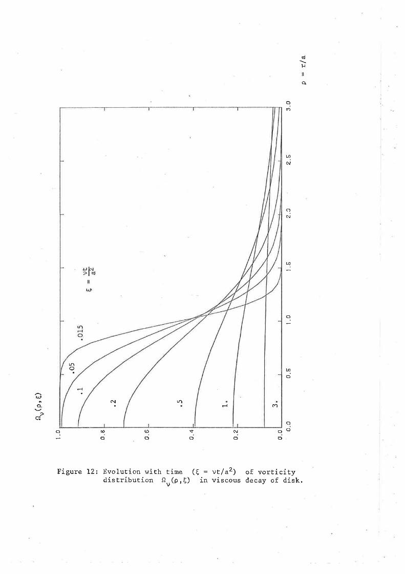
q,

l]ll

o.

c(.'

N

cl(\.,

o

tn()

r¡¡

o.

so

q(f

qo

ct Nlo

c)

c)(]o

Figure 12: Evolution hriÈh time (E = vt/az) of vorticitydistribution nu(0,6) in viscous decay of dísk.

rno

Fl

C\¡ rñF{ Cî

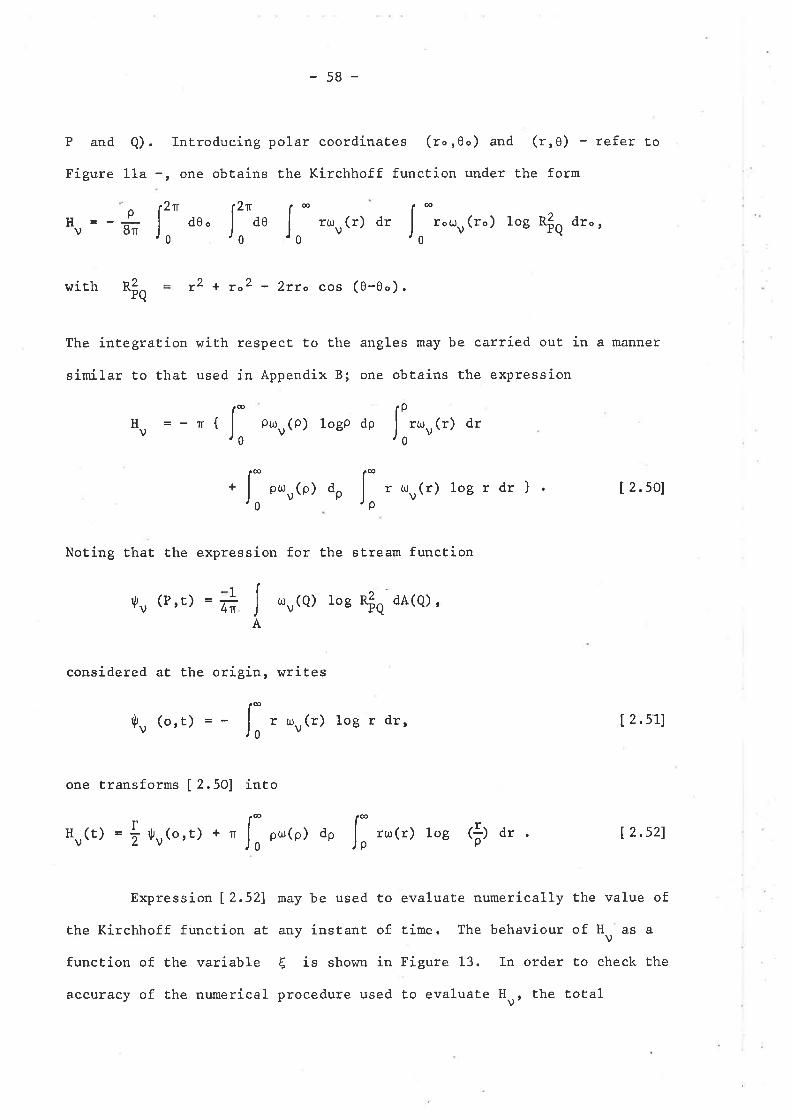
-58-

P and Ð. InEroducíng polar coordinates (ro,0o) and (rr0) - refer to

Figure lla -, one obÈains the Kirchhoff function under the form

ãî' d0" d0 ruJ

Hu --",J;

one transforms [ 2.50] into

(r) dr rou:u (ro) log RfrO dr. ,

2¡¡ 2r @ @

J ,"Co> log Rla dA(Q),

A

pHv =-

0v

0 0 0

with ,2 + ,o2 - 2rro cos (o-0.).

The integration with respect to the angles may be carried out in a manner

similar to that used in Appendix B; one obtains the expression

*lq

ot'ru(0) 1og0 dp ruru (r) drp

0

+

Noting that the expression for the stream function

1úu (P,t) = 4,

considered at the orígin, writes

r- f"I ouru(o) dp I r uru(r) log r dr Ì'o 'p

,l,v (ort) = È I;' ,",', 1og r dr,

[ 2. s0]

[ 2.su

Hv(t) = Ë ru(o,t) . ' f; po(p) dp fl ',,', los (Þ dr | 2 ,s2l

Expressionl2.52l may be used to evaluate numerically the value of

the Kirchhoff function at any instant of time. The behaviour of H, as a

funcLion of the variable E is shown in Figure 13. In order to check the

accuracy of the numerical procedure used to evaluate Hur the total

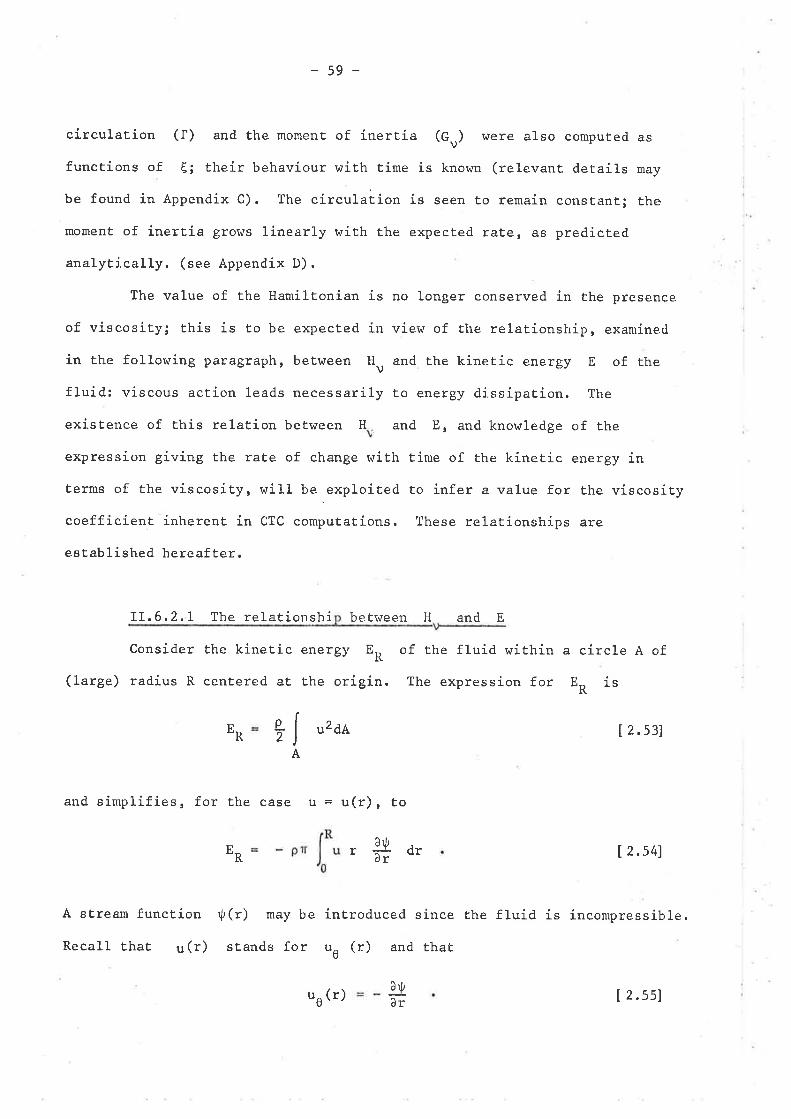
-59-

circulaEion (f) and the moment of inertia (Gu) were also computed as

functions of E; their behaviour with time is known (relevant details may

be found in Appendix C). The circulation is seen to remain constant; the

moment of inertia grohTs linearly with the expect.ed rate, as predicÈed

analytically. (see Appendix D).

The value of the Hamiltonian is no longer conserved in the presence

of viscosity; Ëhis is to be expected in view of the relationship, examined

in the following paragraph, between H, and the kineÈic energy E of the

fluid: viscous action leads necessarily to energy dissipation. The

existence of this relation between H and E, and knor¡ledge of the

expression giving the rate of change wíth time of the kinetic energy in

terms of the viscosity, will be -exploited to infer a value for the viscosity

coefficienÈ inherent in CTC compuËations. These relationships are

established hereaf ter.

If,6,2.L The relationshi between H and E

Consider the kinetic energy En

(large) radius R cenÈered at the origin.

of the fluid within a circle A of

The expression for En is

I 2,531

dr | 2.541

ER

En

rIA

u2dA

and simplifies, for Èhe case u = u(r), to

r 3-U.ðr

A st,ream function

Recall that u(r)

ú(r) may be introduced since the fluid is incompressible.

stands for r0 (::) and that

uu (r) 3-U.âr [ 2. ss]

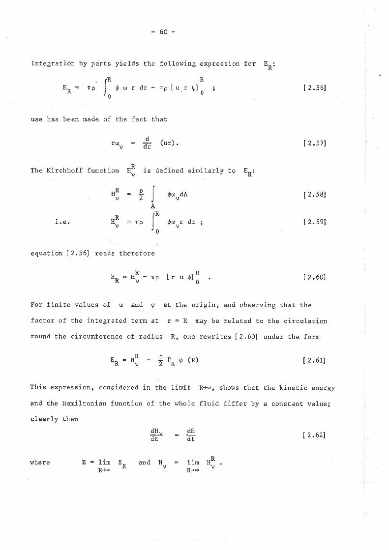
-60-

Integration by parts yields the following expression for En,

R

îp rl o r dr - np [u r rl,]

0

use has been made of the facÈ Ehat

(ur) .

The Kirchhoff function is defined similarly to E."R'

HRv v

ER=R

0| 2.561

[2,571

[2.sB]

dr(l)=vdr

HRv

1.e HRv

dAtft tr,tIA

I

e2

rlurur dr=np | 2,s9)

equatíon 12.561 reads therefore

En HRU

- Trp [r u ú]R

I 2.6010

For finite values of u and ú aÈ the origin, and observing EhaE the

factor of the integrated term at r = R may be related to the circulation

round the circumference of radius R, one rewrites [2.60] under the form

(R) Í 2,6L1

This expression, considered in the limit R*¡ shows that the kinetic energy

and the Hamiltonian function of the whole fluid differ by a consÈanÈ value;

clearly then

dl" = gl t2.621r -ãE

rnú=HT - ÊEn

E=limR-'-

Hv

E'"n 1imR+oo

HRv

where and

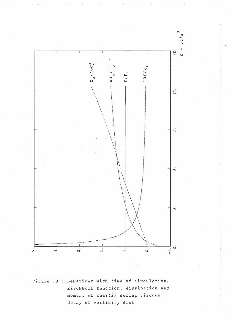
Nqt

+J

{t

f^¡

(\,

o)

(o

co

tn l1 0.t N o ,oI

Behaviour with time of circulation,Kirchhoff function, dissipaÈion and

moment of inerÈia during viscousdecay of vorËicity disk

o>C)o.dt

(-)

o oxxo

ot<

çi\?I

\

I

I

\- --.- \

\

\

Figure I 3

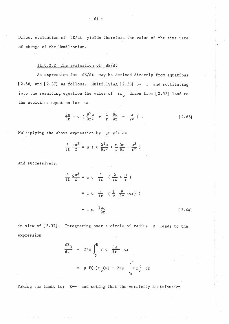
-61 -

Direct evaluation of dB/dt yields Ëherefore the value of the time raÈe

of change of the llamiltonian.

IL6.2.2 The evaluation of d¡/dt

An expression for dE/dE may be derived directly from equations

I2,361 and [ 2.371 as follows. Multíplying [2.36] by r and subtiruring

into the resulEing equaEion the value of rru drawn from [2,37] lead to

the evolution equation for u:

âu¡E=u

ð pu2i'E -t

â2uñ

u12' [ 2.63J( +

âuðr-tt

Multiplying the above expression by pu yields

=u ; ð2u uãu ,t2.1u5[z*;5;-;;z)

and successively:

(

â

âr (ur) )

=uu I 2,641

in view of 12.371, InÈegraÈing over a circle of radius R leads to the

expres sion

dr

p f(R)o (R) - 2rv drv

ô ou2

-+=lltlât 2 P" u

t+aF

!r

Ar.,,.âr

dEn

ã-

â

E

ã

ã?

3gr¿âr

=uu

)

(

2nv ruJ-

0

R

, r2

Taking the limit for R+- and noting that the vorticity distribution

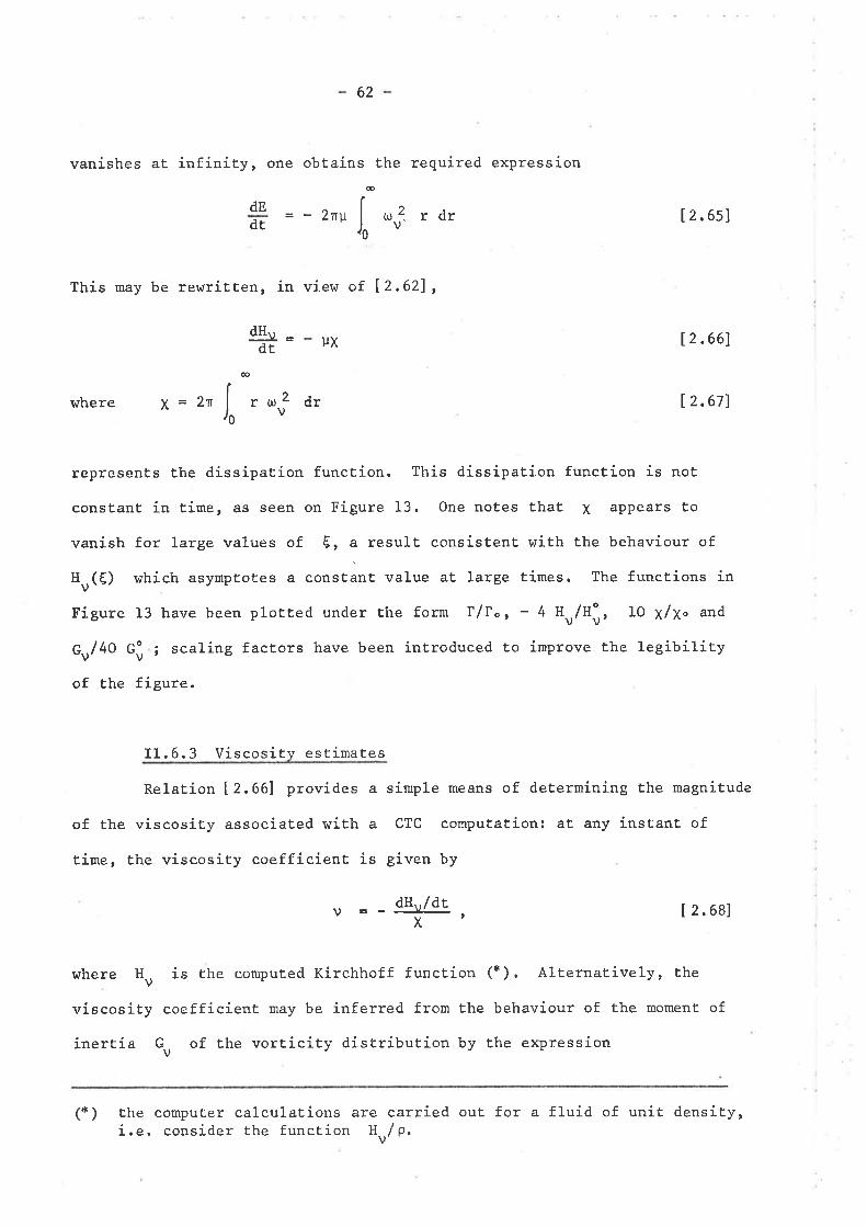
62

vanishes at infinity, one obtaíns the required expressionæ

dE

I= - 2'nv (¡) 2v' rdr [ 2. 6s]

12.661

I 2.671

dr

This may be rewritten, in view of 12,621,

dH.,J=

dr

t ,2 dr

UX

æ

where X=2n

represents Èhe díssipation function. This dissipation function is not

constanÈ in time, as seen on Figure 13. One noÈes thaË X appears to

vanish for large values of E, a result consistenË r,rith the behaviour of

Hv(t) vrhich asymptotes a conslirrt .rr1rr" at, large Èimes. The functions in

Figure 13 have been plotted under Èhe form fflo, - 4 Hv/H;, 10 ¡/¡. and

Cu/40 Gi ; scaling factors have been introduced to improve Èhe legibiliEy

of the figure.

II.6.3 Viscosity estímates

Relation 12.661 provídes a simple means of determining Ëhe magnitude

of the viscosity associaLed with a CTC computaEion: at any instant of

time, the viscosíty coefficient is given by

v _-dHr,/dr. 12,68lX,

I v

where Hu

vis cos ity

inertía G

is the computed Kirchhoff function (*). Alternatively, the

coefficient, may be inferred from the behaviour of the moment of

v of the vorticity distribution by the exp::ession

(n) t,he comput,er calculations are carried out for a fluid of unit densiEy,i.e. consider the function Hv/p.

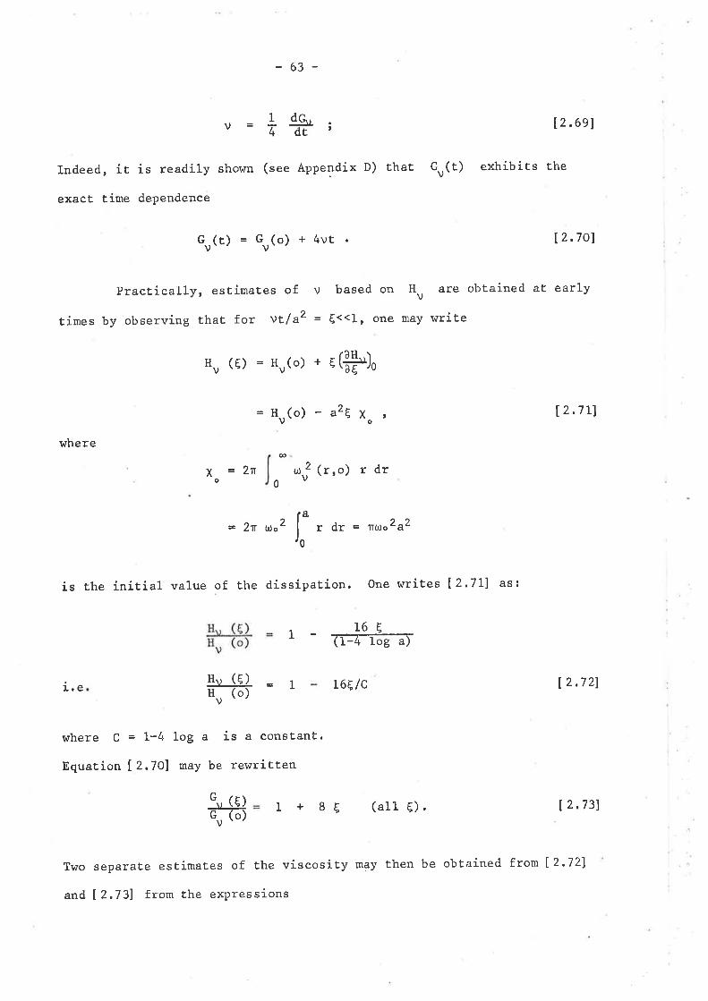
-63-

1 d,C^' : [2.69]v=T,AËt

Indeed, it is readily sho\^7tr (see Appendix D) thaË Gv(t) exhibits the

exact time dependence

cv(E) = Gu(o) + 4vt t2.7ol

Practically, estimates of v based on H, are obtained at early

times by observing thaE for vE/a2 = E<<1' one may write

Hu (t) = Hu(o) . cþ)o

ttu(o) - azE xo , l2,7rJ

where

t.e

æ

X = 2Tro

uru2 (r,o) r dr

f tut =nuo2a2

t6E- G;f-los ãI

1 L6E/c

0

- 2n uo2

is rhe inirial value of rhe dissipation. one writes 12.7Ll 4ù .

1

Hv (E)H, (o)

G', (E)Gu (o)

12 ,7 21

where C=L-4 loga isaconsEant.

Equat,ion l2.7Ol may be rewritten

1+ 8t (all-6). 12,731

Two separate estimates of the viscosíty uray then be obtained from [ 2.721

and [ 2,731 from the expressions

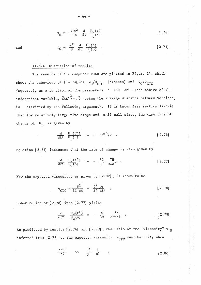
-64-

vH

anda2d

u

uctc

Substitutíon of l2.7Bl into [ 2,77] yields

c.az d H.,(t)16 dt Hu(o) Í2,741

12.7 5l

12.781

12,791

cv(r)Gu (o)ãT8

II.6.4 Discussion of results

The results of the compuEer runs are plotted in Figure 14, which

shows the behaviour of the ratios uH/ucrc (crosses) and ue/ucrc

(squares), as a functíon of the parameters ô and ^t*

(the choice of the

índependent varíab1e, ãAt*'/r^rA being Èhe average distance between vortices,

is clarified by Èhe following argument). It is known (see section IT.5.4)

Ëhat for relatively Large time steps and small cell sizes, Ehe time raÈe of

change of Hu is given by

tt*3 /2 Í 2.7 6)

Equation 12,741 indicates that the rate of change is also given by

v¡1I2 .7 7l

as given by 12.321 , is known to be

dãF-

H., (t* )EF)-

H,, (t* )il6- æ32c

dãF

Now the expecEed viscosity,

ô2 ooTr,t

dã'r-

AE* 4-T-

462æ ¡t--:U

As predicted by resulcs Í2.761 and [ 2.791, the ratio of the "viscosityrr v H

inferred frour [ 2.771 Eo the expected viscosity UCTC tttt be uniÈy when

B 1

azC3 [ 2.Bo]

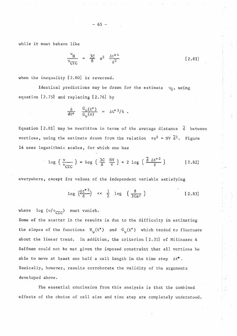
while it must behave like

uH

vctc3c-s-

-65-

dAt* 4

=F

tr"3/4

1og

2 [ 2. B1]

between

Figure

12.821

when the inequality IZ.AOI is reversed.

ldentical predíctions may be drawn for the estimate vG, using

equation lz.lsl and replacing [ 2.761 by

log (þ)= toe (.CTc

log r--)

dãr-

Equation IZ.Af] may be rewritten in terms of the average distance

vortíces, using the estimate drar,rn from the relation Tra2 = XV ã2.

14 uses logarithmic scales, for which one has

ã

3C NVJ-- 'tT

1

z

)+21og(ã ¡r*2---- )

everywhere, except for values of the independent variable satisfying

[ 2. s3]

where log (v/vara) musÈ vanish.

Some of the scatter in the results is due to the diffìculty in estimating

the slopes of che functions Hv(tx) and Gv(t*) which tended to fluctuate

about t,he linear trend. In addition, the criterion [2.31] of Milinazzo &

Saffman could noÈ be met given Ëhe imposed constraint that all vortices be

able to move aË least one half a cell length in the time step ^t+'.

Basically, however, results corroborate the validity of the arguments

developed above.

The essential conclusion from this analysis is that the combined

effects of the choice of cell size and Ëime step are completely understood.

)( B

Tcaz

(o

c,

Figure 14: Viscous effects in the CTC method: dependence ofestimaEed viscosities with tirne step and cellsize. PredicÈions [ 2.80] and [ 2.81.| are shownby dashed 1ines.

N

.o

C{*+J

t€

o-{è0

or-1

I

N

(JHo

orl

Ò¡)o

r-'l

coqI

C)

Oc{ca

?u)(o

?æ

:Æ åF

(JH()

'}F tr ÐF

()H(J

(,

fl{E åF

{+

åFP

{e! {e

åF**ø

*I

*4El

ixI

tr}FÞIItrIIIIIIII

4III

+lþsq

ålF

++

*tr

*

trE

*

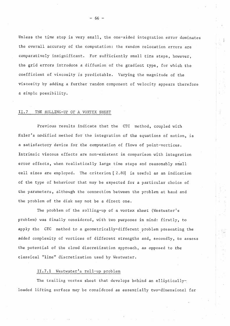
66

Unless Ehe time step is very small, the one-sided integration error dominates

the overall accuracy of Èhe compuËation: the random relocat.ion errors are

comparatively insignificant. For sufiiciently sma1l tíme steps, however,

the grid errors introduce a diffusion of Èhe gradient type, for which the

coefficient of viscosity is predictable. Varying Èhe magnitude of the

viscosity by adding a further random component of velocity appears therefore

a simple possibility.

T.T.7 THE ROLLING_UP OF A VORTEX SHEET

Previous resulEs indicate thaE the CTC method, coupled wiEh

Eulerrs modified method for the integration of the equations of moÈion, is

a satisfactory device for the computation of flows of poinÈ-vortices.

Intrinsic viscous effects are non-existenL in comparison with integration

error effects, when realistically large Eime sÈeps and reasonably sma11

cell sizes are employed. The criteríon [ 2.80] is useful as an indication

of the type of behaviour Ehat, may be expected for a particular choice of

Èhe parameters, although the connection between the problem at hand and

the problem of the disk may not be a direct one.

The problem of the rolling-up of a vortex sheet (l^lestwater's

problem) was fínally considered, with Ewo purposes in mind: firstly, to

apply the CTC met,hod Ëo a geometrically-dífferent problem presenËing the

added complexity of vortices of different strengths and, secondly, to assess

the poËenËial of the cloud díscretization approach, as opposed to the

classical t'1ine" discretization used by l,lestwater.

II.7.1 hlestwaËerrs ro1l-up problem

The trailing vortex sheeÈ that develops behind an elliptically-

loaded lifting surface may be considered as essentially tr¿o-dimensional far

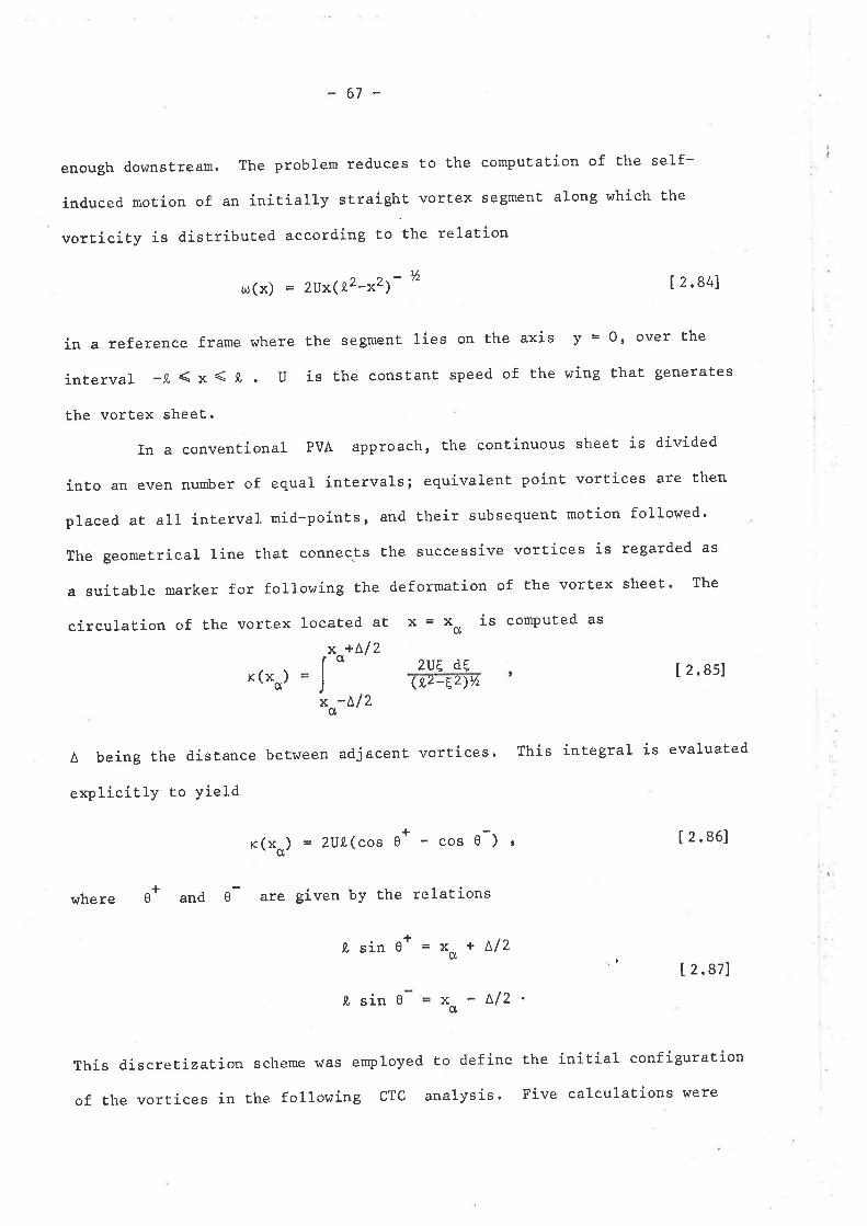
67-

enough downstream. The problem reduces to the computation of the self-

induced moÈion of an initially straight vortex segment along which the

vorticity is distributed according to the relation

t¡(x) = 2Ux( l'2-x2)-tÁ

Í 2,841

in a reference frame where Ëhe segment lies on the axis y = O, over the

interval -L ( x <.e, U is the constant speed of the wing that generates

the vortex sheet.

In a conventíonal PVA approach, the continuous sheeÈ is divided

into an even nurober of equal inÈervals; equivalent point vortices are then

placed at all inÈerval mid-points, and their subsequent motíon followed'

The geometrical line that connects the successive vortices is regarded as

a suitable marker for following the deformaÈion of the vortex sheet' The

circulation of Ehe vortex located at * = *o is compuÈed as

r (xo) l"o*o''xo-L/2

zIJE dE(9.2-Ez)'h

[ 2. Bs]

A beíng the distance between adjacent vortices. This integral ís evaluated

explicítly to yieJ.d

r(xo) = ZtJl.(cos 0+ - cos 0-) , [ 2'86]

where 0+ and, e are given by the relations

0sine*=xo+L/2 .

1 2,87)

.C sin 0 x -A/2'd

Thís discretization scheme \^tas emPloyed Èo define the initial configuration

of the vortices in the following CTC analysis. Five calculations were

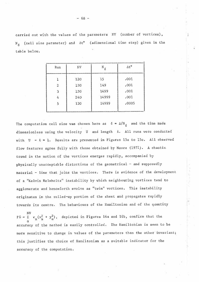
carried out !üíth the values of

Nô (cell size paxameter) and

table belor¡.

68-

the parameters NV (number of vortices),

At* (adimensional time step) given in the

Run NV at*

,001

. oo1

. oo1

.001

. ooo5

The computaEion cell size was chosen here as 6 = A/N6 and the time made

dimensionless using the velocity U and length t, All runs were conducted

with U = !, = 1. Results are presented in Figures 15a to 15c. All observed

flow features agree fully with those obtained by Moore (1971). A chaotic

trend in the motion of the vortices emerges rapidly, accompanied by

physically unaccepEable disÈortions of the geometrical - and supposedly

material - line that joins the vortices. There is evidence of the development

of a "Kelvin Helmholtztr ínstability by vrhich neighbouring vortices tend to

agglomerate and henceforth evolve as tttwint' vor!ices. Thís instability

originates in the ro1led-up portion of the sheet and propagates rapidly

towards its cenEre. The behaviours of the Hamiltonian and of the quantity

NVIG = x ro(x! + y2ì, depicted in Figures 16a and 16b, confirm that the

daccuracy of the meÈhod is easily controlled. The Hamiltonian is seen Eo be

more sensitive to change in values of Ehe parameters than the other invarianE;

this justifies the choice of llamilËonian as a suitable indícaÈor for the

accuracy of the computation.

N^Ò

15

L49

t499

L4999

L4999

1

2

3

4

5

120

L20

L20

240

r20

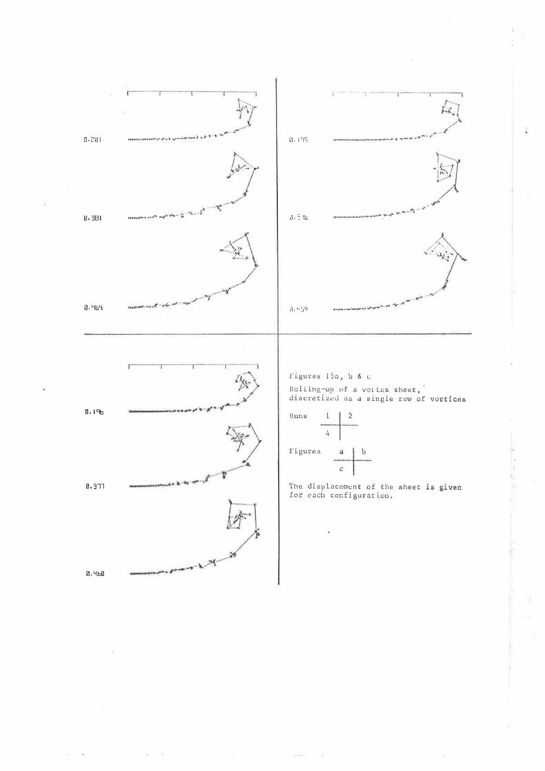
0.¿ør ,..úi#tlii f'dÊ¡¡¡l t,|

ø,38t re\*.r,*rÊ-+*-í

ø, TbT

0. tqb

0. 311

0. Tbø

!1, l(t5 Þ+t st ¡t_-f

ú. l-ltl *l*¡+*È+-* F

!l, \51 Þld.F!r4#â'Ê

l¡iguresl5arb&cIlolling-up of a vortex sheet,rliscretizerl as a single ro$¡ of vor!iceg

,l!¡-l

Runs I

f--]

2

4

I'i gure s a

c

b

The displaceme¡t! of the sheeÈ io givenfor each configuration.

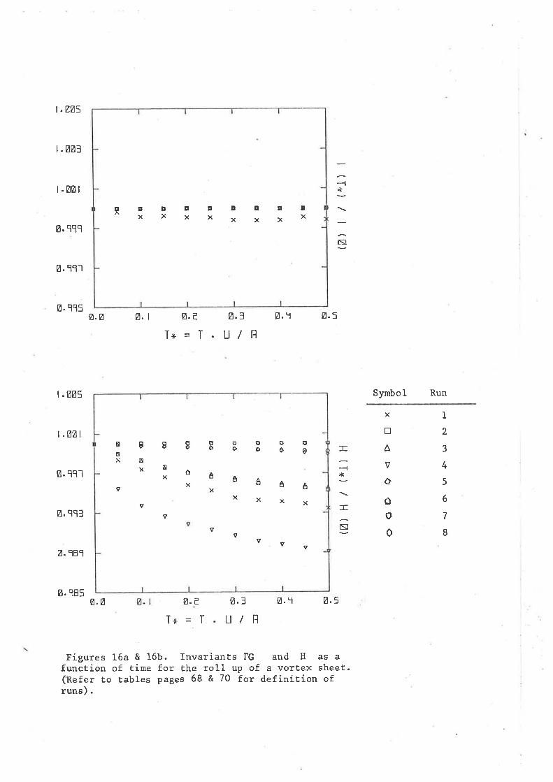
. (sunrJo uortru-rfap ro¡ O¿ S g9 sa8ed saTqef o1 .ra¡a¡)

.faar{s xaf.ro^ e ¡;o dn TTof, al{l roJ aurf Jo uorlcun¡B sB H pue ÐJ stuer.le^ul 'q9T 3 e91 sarn8rg

5'øh'Ø

s'øh'ø

u /nE'ø

u lnE'ø

l-*r2'ø

'1=*le'ø

ø'Ø

t'øø'ø

sBb'ø

IL

9

ç

t7

e

z

ï

sl

-

*.

-

0

ôo

o

^V

trx

bsb'u

Ehh'ø

Lbh.E

tøø'I

5Øn't

Shb'ø

unu Toqu¡r(S

S¡

+F-

Lbb'ø

hhh'ø

tøø'I

Eøø. I

0çoooó ooôôoÊxtr

c

ô

6ô

ôô

6 ô ô

xE

Ê

XE

I

x

I

x

I

x

I

X

I

X

ç

x

q

xE

xE

x¡

xE

XEt

xg

x!

xE

SøZt'I

69-

Failure to model the continuous flor¿ stems not from the computing

method; indeed, it ís knov¡n from Moorers study that the discretization

itself is responsible for the anomalies observed. In a recent work, Fink

& Soh (1978) have convincingly demonstrated that the PVA, as anticipated

by Moore, does not yield a complete discretized form of the integral

equation that, describes the motion of the continuous vortex sheet.

Additional terms that become necessarily large must be taken into accounE,

and radically affect the flow paÈÈern. One is led to conclude that Èhe

conventional PVA used in the vortex sheet roll-up problem is clearly

inadequate. The idea of adopting another type of discretization, based

on Ehe cloud discretization concept, is explored in the next section.

II.7.2 The Cloud DiscretizaÈion Approach

I,iestwatert s analysis, in its classical formulation, bears little

relation to the physical problem. The wing-Eip vortex system generated by

a moving aircraft has necessarily a finite Lhickness; furthermorer the

action of viscosíty diffuses the vortex sheet which soon loses the sharpness

of its initial definition. These physical arguments suggest that the sheet

may be validly discretized using several superimposed layers of vorLex

filamenÈs thaË confer a small, but finite Èhickness to the discretized

system. The evoluEion of the configuration of vortices describes the moEion

of the sheet in a cloud-like manner, and musE be interpreted in the

appropriate, aveïage sense (see Section II.3). In this coarser description

of the flow, the quesÈion of determining the exact geometrical deformation

of the vortex sheet cannoL be clearly answered¡ other g1obal flow features t

however, like the speed of the sheet mid-point, or the raËe aË which

vorticity enters the spiral, are likely to be well approximated.

The cloud discretization idea was tested on the roll-up problem as

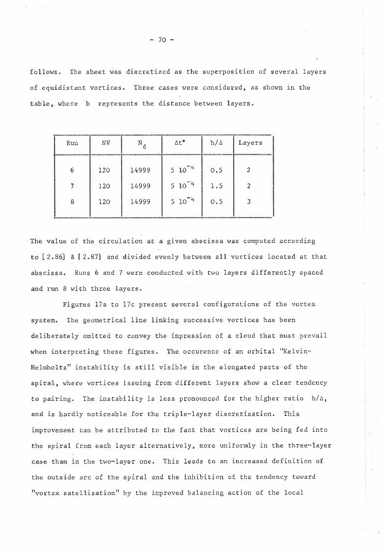
follor^¡s. The sheet vras

of equidistant vortices.

-70-

discreËized as the superposition of several layers

Three cases v/ere considered, as shown in the

table, where h represents the distance between layers.

at* hlL Layers

The value of the circulaÈion at a given abscissa r¡ras computed accordíng

Èo [2.86] &t2.871 and dividea everrly between all vortices localed at that

abscissa. Runs 6 and 7 were conducted with Èwo layers differently spaced

and run B r,¡ith three layers.

Figures 17a Èo 17c presenE several configurations of the vortex

system. The geometrical line linking successive vortices has been

deliberately omitted to convey the impression of a cloud that musÈ prevail

when interpreting these figures. The occurence of an orbital "Kelvin-

Helmholtz'r instability is stilI visible in the elongated parts of Èhe

spiral, where vortices issuing from different layers show a clear tendency

to pairing. The instability is less pronounced for the higher ratio h/L,

and is hardly noticeable for the triple-layer discreEizatíon. This

improvement can be attributed to the fact that vortices are being fed into

the spiral from each layer alternaÈive1y, more uniformly in the three-1ayer

case Èhan in the two-Iayer one. This leads Èo an increased definition of

the outside arc of the spiral and the inhibition of the tendency toward

ttvortex satellisation" by Ehe improved balancing action of the local

2

2

3

Run NV N ¡U

o.5

1.5

0.5

6

7

8

t20

L20

L20

L4999

L4999

L4999

5 10-4

5 10-4

5 10-4

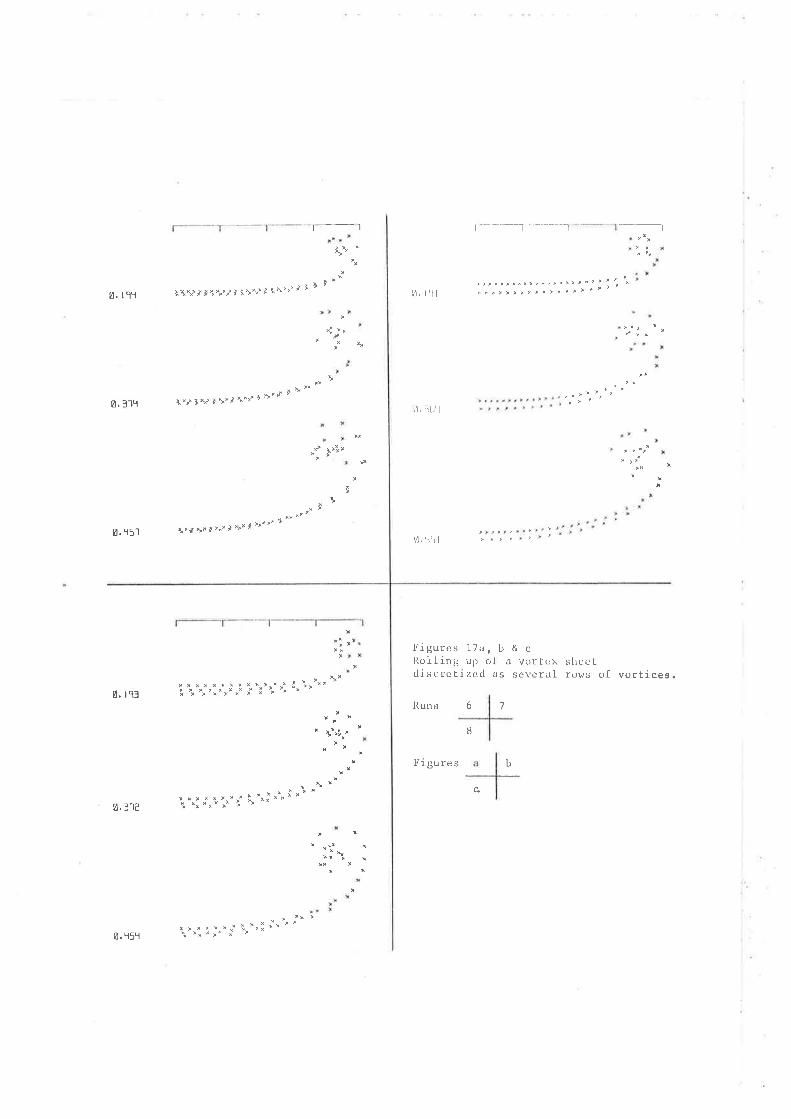
t-l f-__--T___.-.I

>)

ø, t 9.1

ø.l]t1

ø. T5l

ø, r3l

ø.3ï

Irlvli'):,,lì1\ElÈl\>¡>l ì à !'

-n ¡ \o

\x'¡ t x,¡ I * I /,rì, r" r

>l r,

D. rlt

fl. :tir'l

14. .1i t

Ituns 6

'.-,,1 l

}'i*rì>l¡\xl br¡¡ 1

7

b

IigureslTa,b&clì.oILing up ol a vorcox sheet.discrcEizcd as sevcral ro\ds of vortices.

i i'";,:,'"ì"ì i "l"i i i"'"\' *

t ït'ir' 8

Þ'i gu re s

ï',:,¡"1i.i ìo"';"'L c

" rl'

!t

i"'î I ì.' l. i_ ' ¡¡ ¡

ø. r15q

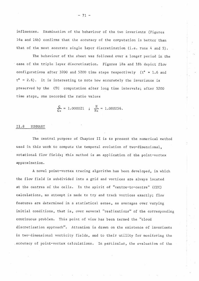
7L-

influences. Examination of the behaviour of the Èwo invariants (Figures

16a and 16b) confirms that the accuracy of the computation is better than

that of the most accurate single layeùdiscretization (i.e. runs 4 and 5).

The behaviour of the sheet was followed over a longer period in the

case of the triple layer discretization. Figures l8a and l8b depiet flow

configurations after 3200 and 5200 time steps respectively (t* = 1.6 and

t* = 2.6). IÈ is interesting to note how accuraÈely the invariance is

preserved by the CTC computatíon after long time intervals; after 5200

time sEeps, one recorded the ratio values

1 .00025 6 .

II. B SIJMMARY

The central purpose of ChapÈer II is to present the numerical method

used in this r¡ork to comput.e the Lemporal evolution of two-dimensional,

rotatíonal flow fíelds; this method is an application of the poinE-vortex

approximat ion.

A novel point-vortex tracing algorithm has been developed, in which

Èhe flow field is subdívided into a grid and vortices are ah,rays located

at the centres of the cells. In the spírit of'rcentre-to-centre" (CTC)

calculations, no aEÈempt is made to Ëry and track vortices exacËly; flor¿

features are determined in a statistical sense, as averages over varying

initial conditions, that is, over several "realizaEions" of Ëhe corresponding

continuous problem. This point of view has been termed the ttcloud

discretization approacht'. Attention is drawn on the existence of invariants

in two-dimensional vorticity fields, and to their utility for moniÉoring Èhe

accuracy of point-vortex calculations. In particular, the evaluation of the

G

Go1.000021 ;

HF-

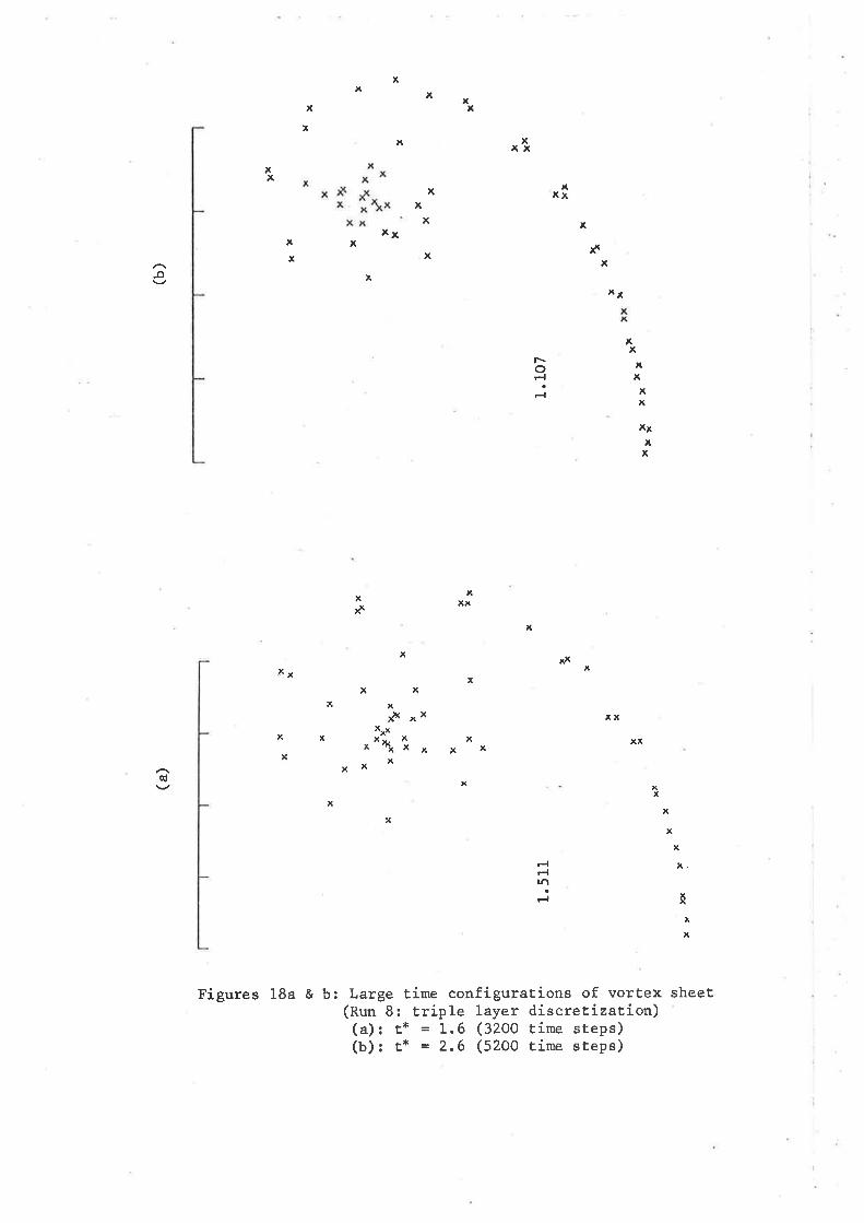
xx x xxx

xx xxx

xx,(x x x

xx T

¡x

xX¡

x

Xxx

",1 i * " *

*

$x xxp

xI

xxxxxx

X¡xx

r\oF{

F{

xxxx*

x

¡X,(xx

x

xx

x

x

xx#

xxx

x xxx

x

xxqt x x

x

18a & b: Large time configurations of vortex sheet(Run 8: tríple layer díscretization)(a): t* = 1.6 (3200 Èime steps)(b): t* = 2.6 (5200 time steps)

xx

x

xx

x.

T

a

x

r.|F{U,ì

F{

Figures

-72-

numerical effects on Ehe energy invariant (the Kirchhoff function or

Ha¡niltonian of the system) appears as a crucial aspect of the CTC method.

The properties of the CTC *åano¿ have been thoroughly investigated

on the basis of the problem known as Rankiners vortex. The essenÈ.ial

conclusion from the resulËs obtained is that the combined effects of the

basic characteristic parameters (ce11 size and time step) are fully

understood; these effects may be quantitatively predicted in terms of their

influence on the energy invariant. The importance of the choice of the

numerical integration procedure is also demonstraEed. The performance of

the CTC algorithm and the relevance of the cloud discretization approach

are illustrated on the problem of hlestwater, the rolling-up of an

elliptical1y loaded vortex sheet. An attracÈive feature of the CTC scheme

ís without doubt its simplicity, which allows the naÈure of the errors

resulting from the various approximations to be explored relat,ively easily.

The centre-t.o-centre method may well constitute a simple ans\,üer to many

problems connected with the point-vortex approximat.ion. The remarkable

lack of sensitivity of integral flow quantities to large changes in cell

size - of itself an intriguing property - strongly suggesËs thaÈ the use of

eomplicated stratagems to remove the singular characEer of the point-vort.ex

velociÈy field (e.g. locally diffusing vortices, Kuwahara & Takami, 1973)

cannot be seriously justified in comparison with t,he simple vortex-relocation

technique of the CTC met,hod. On the other hand, the necessity of employing

an accurate scheme for the integration of the equations of motion has

implicaLions that musE be considered in any point-vorÈex t,racing scheme.

Finally, the ability of the CTC meEhod to preserve all invariants

of the motion presents advantages that cannot be claimed by other available

techniques, in particular r¿it,h alI meÈhods where arbiErary amalgamations are

forced upon the vortices, leading to unavoidable discontinuities in the

73-

value of the invariants. The removal of any ad-hoc mechanism that controls

the amalgamations of vortices is \47ithout doubt anoEher satisfactory asPect

of rhe method.

The proposed computation nethod allows a very significant saving in

computing time, since the velocity of any one vortex becomes a function of

the integer number of x and y - spacings; the function values may be

tabulated prior to any computation. AlËhough the resulting algorithm is

faster than most otherttsummalion algorithmrr methods, it does not match the

computing speed of Fast Poisson Sol-vers. IL is likely, however, that a

combinaËion of Èhe CTC method and a Fast Poisson Solver or a FasÈ Fourier

Transform Eechnique would provide an even more efficient computing code.

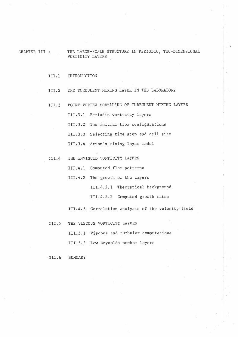
CHAPTER III THE LARGE-SCALE STRUCTURE IN PERIODIC, TIIIO-DIMENSIONALVORTIC]TY LAYERS

III.1 INTRODUCTION

III.2 THE TURBULENT MIXING LAYER IN THE LABORATORY

III. 3 POINT-VORTEX MODELLING OF TURBT]LENT MIXING LAYERS

III.3. 1 Periodic vorticity layers

III.3.2 The initial flow confígurations

III.3.3 Selecting time sEep and cell size

III.3.4 Actonts mixing layer model

III.4 THE INVISCID VORTICITY LAYERS

III.4.1 Computed flow patterns

IIL4,2 The growth of the layers

I1I.4.2,L TheoreÈical background

TIL4.2,2 Computed growth rates

III.4.3 Correlation analysis of the velocity field

III.5 THE VISCOUS VORTICITY LAYERS

III.5.1 Viscous and Èurbular computations

III.5.2 Low Reynolds number layers

III.6 SUMMARY

-74-

III.1 INTRODUCTION

In many free turbulent flows there is a suggestion that some features

arise from the properties of a rota.tiona.L but inuiscid f low. This is the

case for vortex shedding at high Reynolds number, and probably for the- plane

mixing layer which appears Eo be dominated by a quas í-tuo-dímensional, large-

scale structure (Brown & Roshko, L974>. RecenE results (Browand, I97B;

¡Iygnanski eE al, 1978) confirm the large transverse correlaEion scales of

these structures.

The motion pictures of the mixing layer (Brown & Roshko, L974) leave

liÈÈle doubt that Ehe mechanics of the mixing layer is dominated by Ehe

development and int.eractions of rol1er-like sÈructures which originate from

the Kelvin-Helurholtz instabiliËy of the initial vortex sheeE. This impression

is supported by various experimental observations. Browand & trrleidman (1976)

find, at moderate Reynolds number, an essentially two-dimensional flow, ín

which the mixíng layer gror^7s by the pairing of large strucËures; the flow'

whilst not having the three-dimensional velocity fluctuations disÈribuEion

-of the higher Reynolds-number flow (i.e. u'2 = r"), exhibits a Reynolds-

stress similariry. Konrad (lr979) determined a critical threshold Reynolds

number beyond which the small-sca1e turbulent energy experiences an increase

of at leasÈ one order of magnitude, without significant changes in the

estimated growth rate of the layer.

Thus, through in many turbulent flows one deduces from the mean

profiles Èhat the flow is relaÈively viscous to account for the stress, iE

is of interest to ask hor¿ much of this stress results from a large-scale

unsËeady motion of either an irtuíscid rotatíonal fluid, or a ttturbulart'

fluíd (after the Eerminology of Liepmann), i.e. one in which a secondary

small-scale motion can be considered to act like an enhanced viscosiÈy, Yet

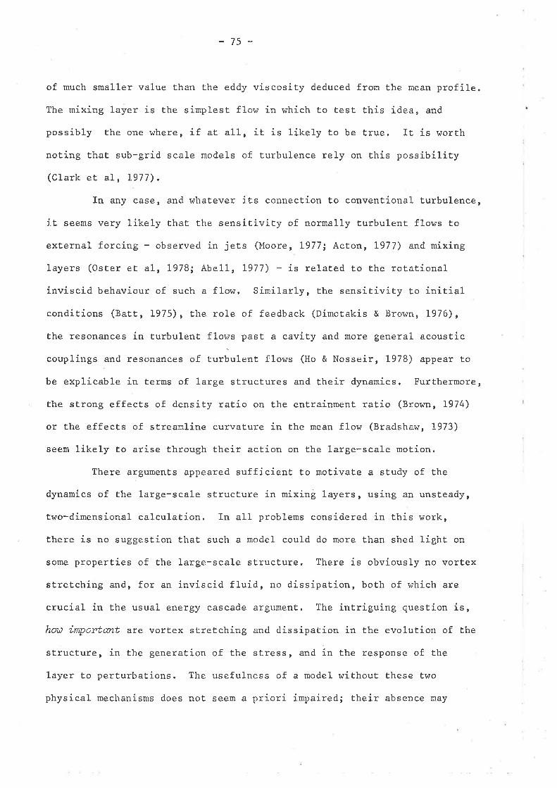
-75-

of much smaller value than the eddy viscosity deduced from the mean profile.

The mixing layer is the simplest flow in which to Èest this idea, and

possibly Èhe one where, íf aL aLL, it is likely to be true. It ís worth

noËing that, sub-grid scale models of turbulence rely on this possibility

(Clark et al , 1977).

In any case, and whatever iEs connection to conventíona1 turbulence,

it seems very likely that the sensitivity of normally turbulent flor^¡s to

external forcing - observed ín jets (Moore, L977; Acton, L977) and mixing

layers (Oster et al, L97B; Abell, L977) - is related to the rotational

ínviscid behaviour of such a f1ow. Similarly, the sensitivity to initial

conditions (Batt, 1975), the role of feedback (Dimotakis & Brown, 1976),

the resonances in t.urbulent flows past a caviÈy and more general acoustic

couplings and resonances of t.rrb,rlent flows (Ho & Nosseir , L|TB) appear to

be explicable in terms of large structures and their dynamics. Furthermore,

the strong effects of density ratio on the entrainment ratio (Brown, L974)

or the effects of streamline curvature in the mean flow (Bradshaw, L973)

seem 1ikely to arise through their actíon on Ëhe large-scale motion.

There argumenÈs appeared sufficient to motivate a study of the

dynamics of the large-scale structure- in mixing layers, using an unsteady,

two-dímensional calculaÈion. In all problems considered in this work,

there is no suggestion thaË such a model could do more Ëhan shed light on

some properties of the large-scale structure. There is obviously no vorÈex

sÈret,ching and, for an inviscid fluid, no dissipation, both of which are

crucial in Ehe usual energy cascade argumenË. The intriguing question is,

hou irnportqnt are vortex sLretching and dissipaLion in the evolution of the

structure, in the generation of the stress, and in the response of the

layer to perturbat.ions. The usefulness of a model without t,hese two

physical mechanisms does not seem a priori impaired; their absence may

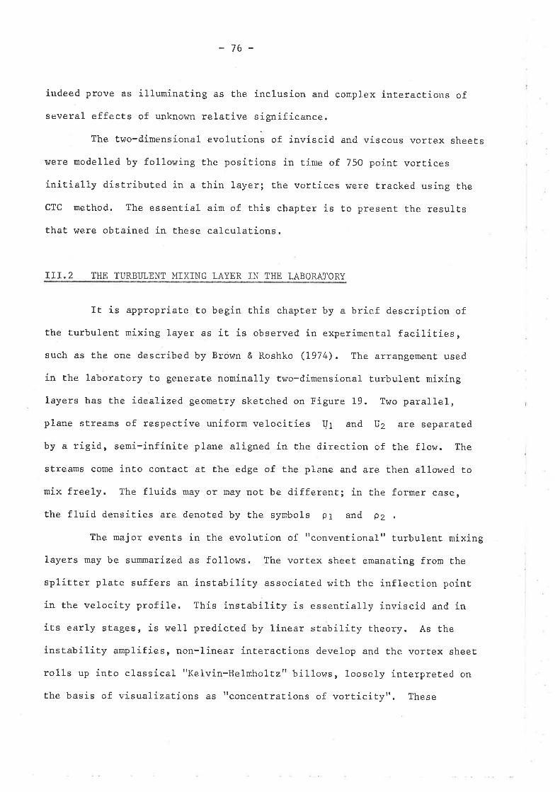
76 -

índeed prove as illuminating as the inclusion and complex interactions of

several effects of unknor"n relative significance.

The two-dimensional evolut.ions of invíscid and viscous vortex sheets

r¿ere modelled by following Ehe positions in time of 75O point vorËices

initially distributed in a thin layer; the vortices were t,racked using the

CTC method. The essential aim of this chapEer is to present the results

that, were obtained in these calculations.

ÍTT.2 THE TURBI]LENT MIXING LAYER IN THE LABORATORY

It is appropriate to begin this chapÈer by a brief description of

the Eurbulent mixing 1.ayer as it is observed in experimenÈal facilities,

such as the one described by Brôvrn & Roshko (L974). The arrangement used

in the laboratory to generate nominally two-dimensional turbulent nnixing

layers has the idealized geomeÈry sketched on Figure 19. Two paral1el,

plane streams of respective uniform velocities U1 and lJ2 are separated

by a rigid, semi-infínite plane aligned in the direction of the flow. The

streams come inÈo contact at the edge of the plane and are then allowed Èo

mix freely. The fluids may or may not be different; in the former case,

the fluid densities are denoÈed by the symbols pI and p2

The major events in the evolution of "conventional'r turbulent mixing

layers may be summarized as follows. The vortex sheet emanating from the

splitter plate suffers an instability associated \^/ith the inflection point

ín the velocíty profile. This insEability is essentially inviscid and in

its early stages, is well predicted by linear stability theory. As the

instability amplifies, non-linear interactions develop and the vortex sheet

ro11s up into classical "Kelvin-HelmhoL|ztt billows, loosely interpreted on

the basis of visual-izations as "concentrations of vorticity". These

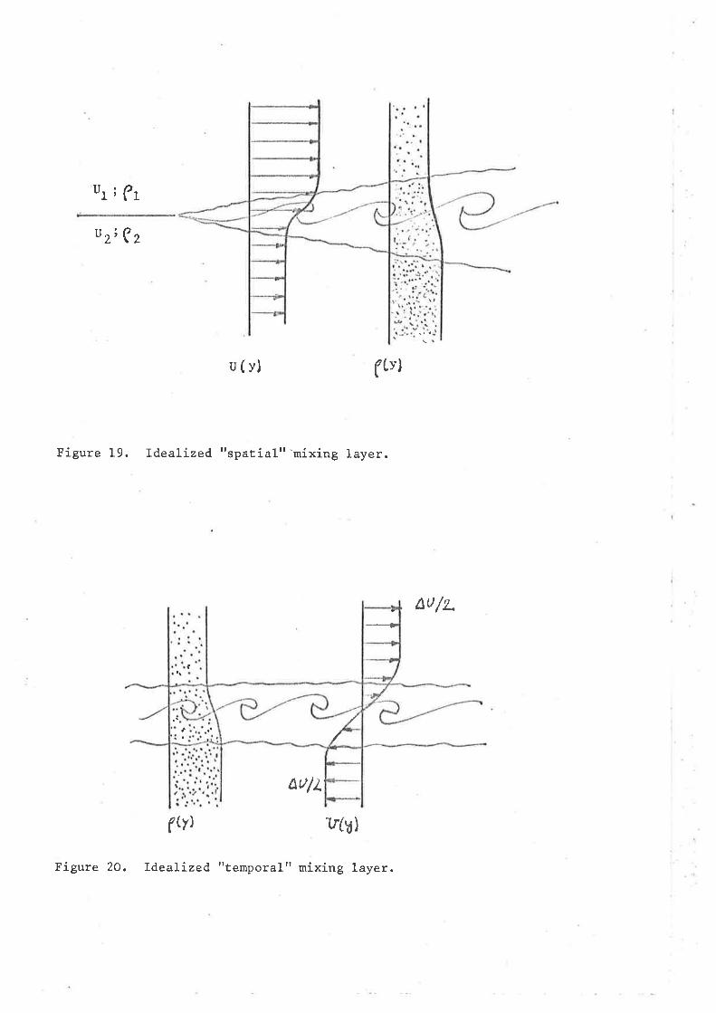
ur;ßr

uzr(z

u(v)

Figure 19. Idealized "spatíal"'mixing layer.

I

(Lv)

aa/z

aul¿

((Yt I¡(u)

€

Figure 20. Idealized "temporalt' mixing layer.

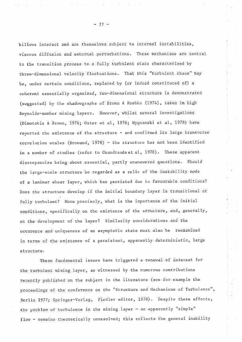
-77

billows interact and are themselves subject to internal instabilit.ies,

viscous diffusion and exÈernal perËurbations. These mechanisms are central

to the transition process to a fully turbulenE state characterízed, by

three-dimensional velocity flucÈuations. That this ttturbulent chaostt *.y

be, under certain conditions, replaced by (or indeed constituted of) a

coherent essentially organized, Ëwo-dimensional strucEure is demonstrated

(suggested) by the shadowgraphs of Brown & Roshlco (1974), taken in high

Reynolds-number mixing layers. However, whilst several investígations

(Dimo¡akis & Brown, L976; Oster eE al, I97B; l{ygnanski et al,1978) have

reported the existence of the structure - and confirmed its large transverse

correla¡ion scales (Browand, 1978) - the structure has not been identífied

in a number of studies (refer to Chandrsudaet al, 1978). These aPParent

discrepancies bring abouÈ essential, partly unansl^/ered questíons. Should

the large-scale structure be regarded as a relic of the instabiliEy mode

of a laminar shear layer, whieh has persisted due to favourable conditíons?

Does the structure develop íf the initial boundary layer is transitional. or

fully turbulent? More precisely, r,rhaÈ is the importance of the initíal

condí,tions, specifically on the exisEence of the structure, and, genetalLy,

on the development of the layer? SimilariLy considerations and the

occurence and uniqueness of an asymptotic state must also be reexamined

in terms of the exisEence of a persistent, apparently deterministic, large

s t ructure .

These fundamental issues have triggered a renewal of interest for

the turbulent mixing Layer, as witnessed by the numerous conEribuEions

recently published on Ëhe subject in the liEerature (see for example the

proceedings of the conference on the "SErucEure and Mechanisms of Turbulence",

Berlin L977; Springer-Ver1ag, Fiedler editor, 1978). Despite these efforts,

the problem of turbulence in the mixing layer - an aPparently ttsimplet'

flor¿ - remains theoretically unresolved; this reflects the general inability

-78-

of present analytical theories of turbulence to cope with real flow situations.

A study of the evolution of vorticity. layers, in which the essential charac-

teristics of the large-scale strucEure, two-dimensionality and Reynolds-

number independence, al.e imbedded, appears therefore well worth while in

the context depicted above. The following sections show how the problem \^ras

tackled in the scope of the point-vortex approximation.

III.3 POINT-VORTEX MODELLING OF TURBI]LENT MIXING LAYERS

III.3. 1 Periodic Vorticity Layers

The rrturbulentl' character of Ëhe mixing layer in an inviscid, tr,ro-

dimensional fluid was first recognized by KadomÈsev & KosËomarov (1972).

Their numerical, point-vortex si,ray of the spaÈial problem was, however,

unable to uncover the exisÈence of a large-scale structure. (It ís in fact

interesting to note that they identify the turbulent character of the layer

by referring Eo the absence of attregular chain of vorticesttin the computed

flow configurations.) The lack of evidence of an organized vorEex structure

in their computaEions may be attributed to various factors. There is,

first, the poor resoluËion in the definition of Èhe vorticity fíe1d

connected with the limited number (1oO) of vortices used in the discreti-

zatíon of the free shear layer. The presence of an absorbing r¿all - normal

to the direction of flow and placed some distance downsÈream of the

ttsplitter platett edge, necessary to limit Èhe extent of the computation

interval , introduces boundary . ef f ect s of unknor^¡n importance .

Finally, and more imporËantly, there is the possibility that the technique

employed for the shedding of vortices at the parÈit,ion trailing edge was

critical Eo the subsequent layer development (see ClemenEs & Maull, 1975),

These uncertainties illustrate the intrinsic difficulties associated with

79-

the modelling of the spatial problem. In order to avoid the complexiÈies

brought about by the presence of boundaries, consíder the following problern

(refer ro Figure 20).

Imagine an observer attached to a Galilean reference frame moving

downstream with a convection velociËy U, = %(U1+Uz). This observer sees

the growth \^rith time of a turbulent shear layer dríven by a velocity

difference AU = UI - U2 . The míxing layer flow, viev¡ed in Ehis different

perspective, can be idealized as follows. Two half-p1anes, filled with the

same fluid or with fluids of different densities, are separated by a

membrane set on the axis y = O. In both half-spaces, motion is taking

place with uniform velocities, UI = LIJ/2 in the upper half plane,

lJz = - AIJ/Z in the lower half-plane. At some initíal instant, the membrane

is suddenly removed, creating an unstable interface, effeeËive-ly a vortex

sheet of strengËh AU per unit length, which will deform and eventually

become ËurbulenË, fot any small initiaL perturbaËion in the case pL = pz

or spontaneously for pt * pz . This idealization defines the tentporaL

pz,obLem, The modelling of the temporal problem amounts, therefore, to Èhe

computation of the self-induced motion of an infinite, perturbed vortex

sheet.

CompuEaÈions of finite-lengÈh vorticity layers suffer from a major

disadvantage: the ends of the vortex sheet ro11. up, resulting ín strong tip

vorÈices Ëhat induce rapidly unacceptable distorÈions of Ehe whole velocity

field. IË is more satisfactory to consider infiniÈeIy-periodíc vorticity

layers, generated by the cyclic repetition of a layer of finite lengÈh.

Periodic vorËiciEy disEributions ur'(x,yrt) satisfy the requirement that

urn(xryrt) = on(x + nlryrt) (n = 1 ,213 r, ..)

L being the length of the basic definition ínterval.

[¡.L]

-BO-

IÈ is clear, in view of [3.U and [1.54] - [1.55], rhar row-

vortices provide a suitable means of discretizíng periodic vorticity fields.

The motíon of a cloud of NV to"-.rorti"", initially at rest in a given

configuration ( (*;,fi;rl) specified) is obtainecl by numerical inregrarion

of equations [ 1.56] .

The simplicity of the surmaÈion algorithm for row-vortices is, in

conventional tracing methods, heavily penalizecl by Ehe computatíon load

that arises from the (costly) evaluation of the hyperbolíc- and circular-

function terms in formulae [ 1.56]. The CTC method drastically reduces

the computing effort by allowing Èhe pretabulation of these Èerms. DisLances

between vortices in Ehe CTC method are necessarily multiples of the cell

síze, so thaË

X^=ôxlJdÞ 'd ß clß

J )=ôxJI 3.21

Yoß = ôy(Ia - ts)oß=ôyI

The integer JoÊ (roß) takes any of the possible values 0,L,2r...,NG-I

(MG-l) , if Èhe compuÈation grid has NG columns and MG ror¡/s. The

functions .i., 4 xou {"o, f xo') and sinn 4 vo' (cosh * t"U) rake

accordingly any of NG(MG) possible values, which need be computed only

once and stored in a table for further, quick reference (typically

NG & MG - 5000). This procedure reduces Èhe central processing time by a

facÈor of Ëhe order of 1O (CDC 6400 computer).

III.3.2 The initial flow confiRurations

Two of the serious criticisms that have been made about vortex

modelling studies of Eurbulent flows refer Ëo the lack of "predíctive

abilityil of the method, and to the questionable validity of íts rrpost-

-81 -

dictions" in view of tl're arbitrary choices for the vortex interaction 1aw

and for the method of simulating diffusion effects (Saffman, 1977). A

constant concern in this study has bàen not only to reduce the arbítrariness

and uncertainties of the method by avoidíng the use of ad hoc computation

stratagems, but also to Ëry and assess the predictive ability of the PVA

by minimizing the amount of information fed into the model about the

phenomenon to be investigated. The choice of appropriate, realistic

initial flow configurations is an important step of the modelling process

and was guided by the following considerations.

It is argued in linear stability theory Ehat arbitrary perÈurbations

(of a basic flow configuration) may be viewed as the superposition of

ttnormal modes" and that sEabitity characËeristics are, consequenÈly, suitably

anaLyzed in Ëerms of elementary Fourier components (see for example

Chandrasekhar, 1961). This approach has prevailed in mosË poinË-vortex

studies of the infinite vortex sheet problem, where the initial configura-

tion consists of a sinusoidal perturbation (Rosenhead, 1931; Zalosh , L9763

Acton, I976). An alternative point of view has been adopted here. Initial

confígurations are obtained by randomízíng the positions of the vorti,ces

wirhin a narrov/ strip along the interface, as shown on Figure 21. The

random element in the initial conditions is introduced at tvro distinct

levels. Initializations of the first type - "type-I flor*s" - are charac-

terLzed by a uniform circulation per unit length: the randomization only

affects Èhe lateral positioning of the vortices. Initial conditions of the

second type - t'Eype-II flows" - are ful1y random : they present non-

uniformities in circulation per unit length as well as in the lateral

positioning of Ehe vortices.

Randomized vorticity distributions provide a reasonably unbiased

starting poinÈ Ëo investigate the possible universal character of vortical

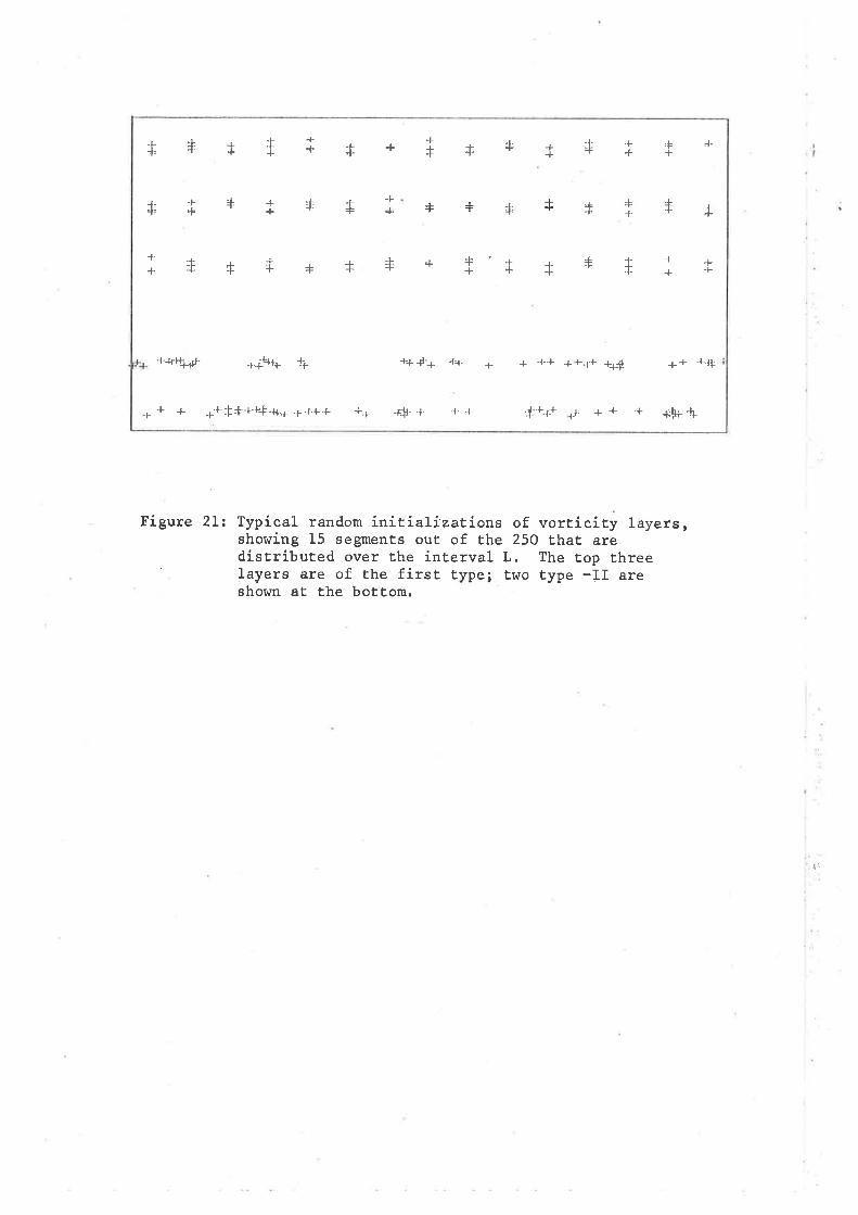
ìl

Iuoffoq eqf lE lI¿lIoqSeJE II- ad,{1 on1 faddf lsrT} eqf Jo erE sreiBT

êar,qf do1 aq¿ ..I IBA¡aluT aql tê^o pafnqTrlsrparE leq1 oçz aql Jo fno sluauSas ç1 Surnoqs

's.r,aÍe1 .dlrcrlron to suorlBzrIETlTuT rrropuer 1ec1dÁ¿ :1¿ arntrg

q^+ü* +. 1- -l- -+:r 1:ri.-f-r- +. +--È+ -r-¡- l-++t- +'H-.f+¡ +lr-f.r- +. + r-

#+ +* ¡f:l-1 1Ì'-r-t' +-r. + + -r.¡ +-É++++ +r*.rit- ¡ftr+*

+i++tf+++++++f+-f

t rl.+

-+

++++++++-

++++

+1-

++1,

++.t

+++++

+*fir++

82

large structures: Ehe Fourier compone.nts of the perturbation fields at

flow initiation cover, in principle, an extended range of wavenumbers.

It is therefore inËeresting to consíder the ouEcome of Ehe instability

mechanism ín the light of linear instability theory. A further justifi-

cation for the choice of initial conditions is found in the observation

Èhat random distributions of vorticity emerge spontaneously from initially

uniform, unperturbed vorEex sheeEs under the actíon of viscosity (this

action being equivalent to random displacenents of vorÈices in the

discretized system).

In selectíng these initial conditions, it also seemed important to

have very large aspecË ratios (length of cyclic inEerval L : initial

vortieity thickness O;) to try and avoid subsEanti.al effects due to the

periodic interval. The use of a large number of vortices \¡Ias necessary to

achieve a reasonable visualization of the vorticity regions. Specific

type -I and type -II flows t,/ere generated as folIows. The cyclic interval

was divided into 250 equal lengÈhs. In type -I flows, lhree vortices were

placed at the middle of each of the 250 segments (to give the uniform

circulation per unit length); their vertical positions were chosen from

14 possible locations in a toLal height equal to approximately one-half of

the segment length. In Èype -II f lows, the 750 vortices \¡rere allocated in

a fully random qray over the 250 segments and within a height of L/4 of. a

segment length. A standard random number generator was used to obÈain

the uniformly distributed random numbers, Two type -I and three type -II

flows were studied; Ehe layers $rere follor¿ed until Èheir aspect ratio

dropped at Ehe most to a value of 3 (typically, not less than 10).

-83-

III.3.3 Selecting time step and c.ell size

The choíce of time step was guided by considerations about a1lowab1e

changes in Lhe energy invariant of ttrà system of vortices during a complete

calculation. Order of magnítude estimates for AH/H. may be obtained from

a generalizatíon of the results obtained for the test case of Rankiners

vortex. This required interpreting the adimensional tíme previously used,

t* = Euo/2 (see section II.5.3), in terms of the charact,erisEic roÈation

period "t = d2h of neighbouring vortices (d is the average distance

between the vortices; y is the vorEex strengEh); clearly t* = E/2r,

Observing thaE the calculations are to follow the layer development over

a range of aspect ratios going from an initial value L/ôi - ZOO to a

final value f/ 6f, - 20, and anticipating a temporal growth for the

vorticity Èhickness of the order of

tuAH

OJ

J(¡)

(T*

- 5 6f / ô"-(¡ûj

T*

ttõ'

t*rJ, t 3.31

one may estimate the duration Tf of a complete computer run to be

approximately

$lrAU) tAUôo

5t 3.41

Using Ehe two relationships

NVd2= 6"L LAU / NV, t 3.sl(¡)

one obtains the estimate

t3.61

typically, using Ehe representative figures given above, one obtains

1* : 50. The time rate of change of the Kirchhoff funct,ion may reasonably

;Y

-84-

be expecEed to be of the order AE*3/2

Èotal ehange in H is approximated by

over the time interval T*, the

: ¡ ¡¡* 4/2 I g.z]

where N is the number of tirne steps. Limíting the number of time steps

to 1500 by choosing At* = 1/3O leads to a total variation in H of the

-âorder of 2 LO-"; this choice of At* r.r¡as retained as an adequate

compromise between accuracy and computaËion cost.

The choice of ce1l size is to some extent arbiÈrary; it affeets

only the size of Èhe arrays for Èhe tabulated circular and hyperbolic

functions, and the magnitude of the implicit viscosity ucTC. From [ 2,3o]

and [3.5], the expression for vCTC is readily found to be vCTC =

ô2 ¡U / z+ 6', At*. A characteristic Reynolds number may be formed:

Re 24 [ :. aa]

and rewritËen, using ô = LÂ{G, AS

Re = 24 Atx NG2^OgaL [ 3.8b]

Selecting a Eypical value NG = 825O (and using At* = L/3O), one estimates

the initial and final Reynolds numbers to be

RE: 1360 , J" = 13600 . t3.91

Reynolds numbers recorded in the actual computations ranged from

RE: 15OO to Je * 75,OOO. With this value of the viscosity, the diffusion

contribuËion to the total growth of the layer compared with that of Lhe

inviscid processes is estimated to be 17" only; in fact, changes in the

Kirchhoff funct,ion were of the order of. 67. after 1200 time sÈeps, a variaÈion

AHH"

0 ô" Ar* /ô2

(+)

üJ

)i

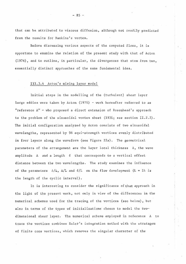
-85-

thaË can be attributed t,o viscous diffusion, although not readily predícted

from the result,s for Rankiners vorEex.

Before discussing various aspècts of the computed flows, it is

opportune to examine Ehe relation of the present study with that of Acton

(1976), and Ëo outline, in particular, the divergences thaË stem from two,

essent,ially distinct approaches of the same fundamental idea.

III.3.4 Actonrs míxing layer model

Initial steps in the modelling of the (turbulent) shear layer

large eddies were Èaken by Acton (7976) - work hereafÈer referred to as

ttreference At'- who proposed a direct extension of Rosenheadts approach

Èo the problem of the sinusoidal vortex sheet (1931; see secÈion fT,2.2).

The initial configuration analyzed by Acton consists of two sinusoidal

wavelengths, represented by 96 equi-strength vortices evenly distributed

in four layers along the waveform (see Figure 22a). The geometrical

parameËers of the arrangement are Ëhe layer local thickness A, the wave

amplitude A and a length ô chat corresponds to a vertical offset

distance between Ehe two wavelengths. The study examines the influence

of the parameters A/1,, A/L and ô/L on the flow development (L = 2À is

the length of the cyelic interval).

It is interesÈing to consider the significance of that approach in

the lighE of the present work, not only in view of the differences in the

numerícal schemes used for the Èracíng of the vortiees (see below), but

also in terms of the types of initíalizations'chosen to model the two-

dimensional shear layer. The numerical scheme employed in reference A to

trace the vortices combines Eulerrs integration rneËhod with the stratagem

of finite core vortices, which removes the singular character of the

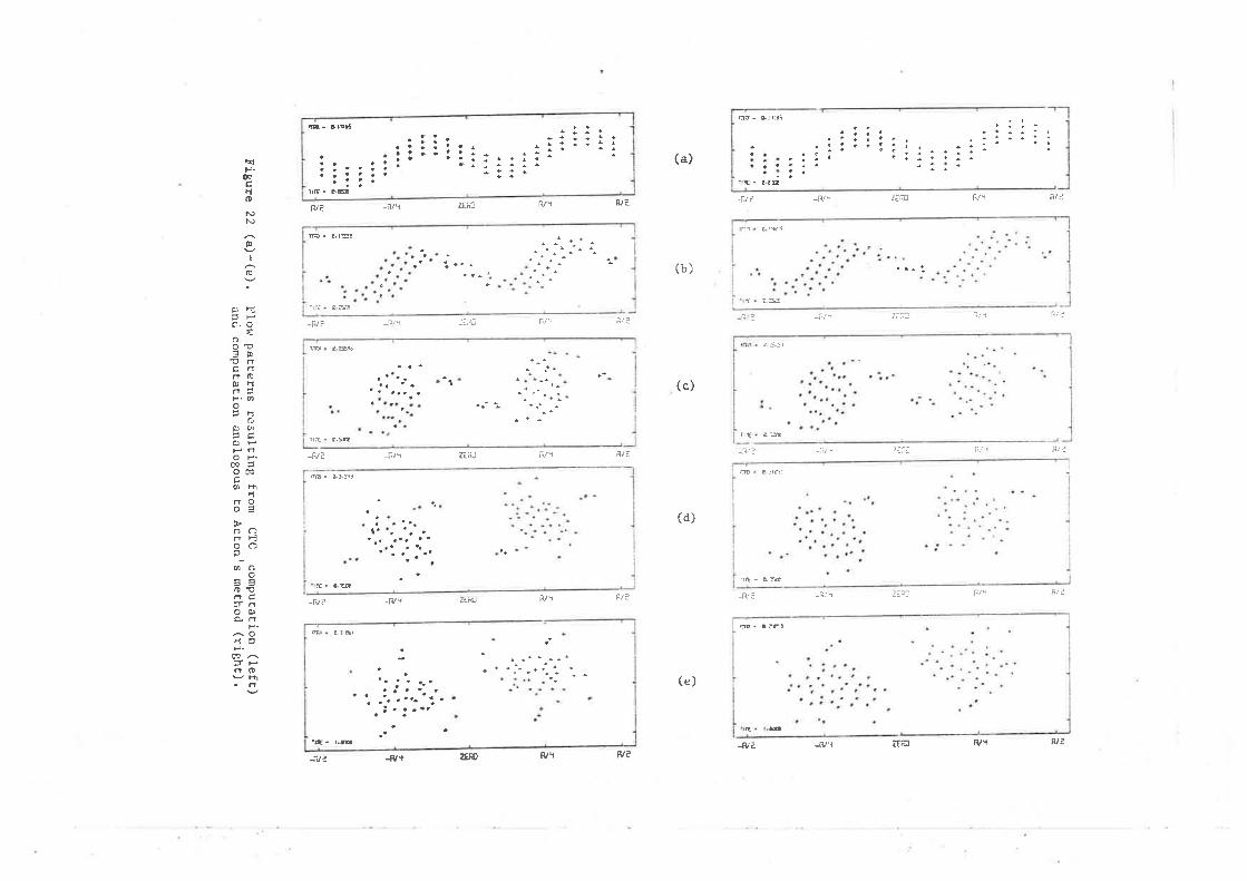
-ß/e

E. ¡,¡e8

tr i¿ a -¡7

-lì/-

ö öÍò

tf, Ltç

-Èe

¿l¡ai

t rÞ

-tì/ ¿

È¡ròr

'E- r.E

-Rr/T

-$/r

-lì/Y

¿E,î!

: .-.

::iri

nt- gll;ll

G:

Ìtf, !.Ð

-¡/'¿

a ¡rð:

-ru¿

¡¿u

-fv¿

(a)'llts.

0çÉHoNl.J

a

r[-ß/¿

n/¿

lit ¿

Fi¿

A/a

Gt1

t !cì

. i¡:

1:41

tì/\

tì/ \

B/¿

f,,r¿

Êt?

(b)

(c)

(d)

(e)

-ß./!

-iì1r

-iìl I

_Ê,,1

Þ

I

o

ÞÈio-oo

=0,'ÉrçñnoÞrlñÞP.ØoÞÈl

oÊlø

ÈHPToH.oaÞo0açøHì

nnOoãÞoc)rÊoa)

Øôo

otÌÉifao0)ê-r

ts.aOFlÞ

ÛaÍFñO

lìl1

ß/r

. '.-'-..-.: '. -

zacJ

ZEP;G/\

lrE- 0.6

EE

Ne.fl,/9¡rel-fv'r-At ¿FI?Fr'I¡¡no{/{-itz

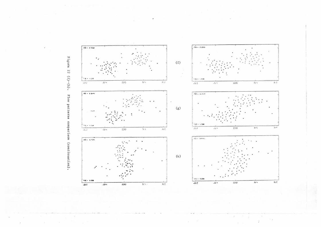
F' ¿EÞ

[5t

-ru¡

-R¿

-lVr

-å/ I

zE.!

z[g]

(f)

(e)

(h)

-lì ¿

-lì/ ¿

-l.V'r

-tv1

z?ll0

zÉ;?0

lì./ I

c/ì

F,' T

F/¿

At¿

ll/ I

ll/ | Fl¿

¡d

caÊIoT..J

¡J

Ht

I

Èrl

o{'o0¡nFo|lâØ

oo4ÞÈt

6o

ooÞrtsrâÞñF.o

4¿

fæ

6- tÐ

€@EE

¿Ðr,G

G . fnlJ

E- ¿Ð

. -t-:.: .';- l'.

ZERiI-Â/r.at¿Ai,:¡æ€T

-86-

discretization (proposed by chorin & Bernard, L972; see section fi.2.2),

It is particularly illuminating to compare the outcome of a CTC

analysis (using Eulerts modified method and no explicit numerical artifice)

of the sinusoidal, two-wavelength problem r¿irh that of the method of

reference A (* ) . A typical example of comparative runs is proposed in

Eígure 22. The flow configurations in the right-hand side column correspond

Èo run I of reference A (A/À = O.I5i A/^. = 0.10; ô/À = 0,0375;

^t* = otlu- = 0.0125). The left-hand side flow patterns were obuaíned by a

crc analysis using a square cell (o/l = s ro-4¡ and keeping the same

value for the Eime step At*. The obvious discrepancies Ehat emerge, as

the computat,ions proceed, lead rapidly to fundamentally dissirnilar flows

(see paÈterns (h)). The accuracies of the numerical procedures are compared

in Figure 23 ín terms of Hamiltonian conservation. The pronounced loss of

invariance (8oZ over the time interval considered), imputable to the

numerical meÈhod used in reference A, is clearly reflected in the diminishing

compacÈness of the vortex clouds and is a direct consequence of Èhettbulk

diffusiont' effecE characterist,ic of Eulerrs integration method. One is

therefore led to conclude that Èhe validity of Actonrs modelling appears

questionable, and that some of the results given in reference A may

require a careful reassessment.

The choice of a simple sinusoidal initialízalíon appears justifiable

in an attempt to isolate the basic païameters that influence Ehe rolling-up

process: one may, however, anticipate t.hat. periodicity (i.e. boundary)

(*) rhe flow configurations of reference A were used to choose theparameters of a CTC eomputation based on EuLerts method. Thisprocedure was found to give results in close agreement rvith those ofreference A, and was consequently retained as a satisfactory substiEutefor Actonrs calculation method. Actonts method could not be duplícatedexactly due to a lack of kno¡+ledge of the core radius value used.

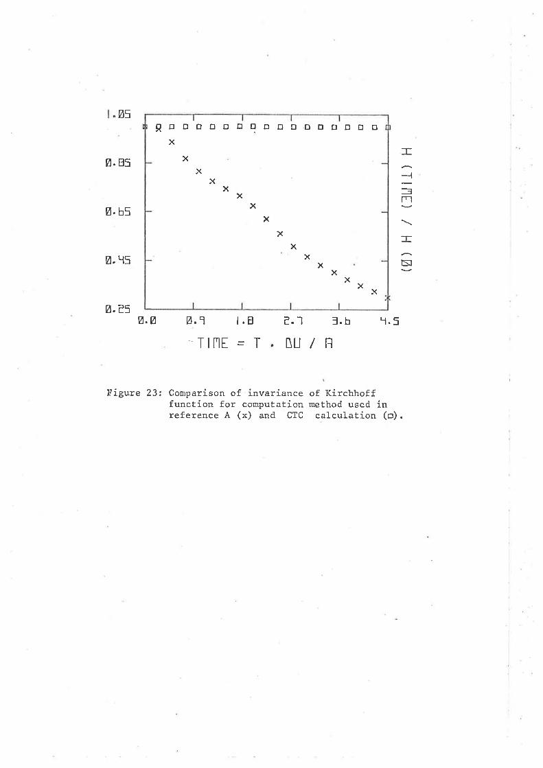
ø5

ø. B5

Ø.b5

Ø. ïs

Ø. e5

:tr

:=11-]

:tr

N

ø.ø t.E d.r

ßu/3.b

u

El,1

TINE

ï.5I

Fígure 23: Comparison of invariance of Kirchhofffunction for computaEion method used inreference A (x) and CTC calculation (o).

RtrDDtrOOOoE¡E¡DtrOtrDtrx

xx

xx

xx

xx

XX

xx

x x x

-87-

effects become non-negligible as soon as the two vortex clouds that emerge

from the sine waves amalgamate int.o a single central sÈructure: Èhis is

likely to seriously restricÈ the time'interval over which the computation

may be Eaken as being "realistic". This argument is supporEed by the

anomalous behaviour of the gro\,\rth of the layers at the late st,ages of the

computations (see reference A, Figure L7), In this respect, it ís

significant to point out t,hat, in the presenE study:

(a) all layers possess an extremely large ínitial aspect ratio (L/ô; - 250);

(b) all computations terminate when the flow patterns consist of only a

fer¿ structures or, equivalently, when the layer aspect ratio drops

down to values in the range of 10 to 3. This order of magniËude is,

in eontrast, typical of the ínitiaL configurations examined in

Reference A;

(c) the ability of witnessing as many interaction events as possible is an

essential feature of the present investigation; this capability is not

íncluded in the computations of Acton, which concenÈraÈe on a single,

particular pairing event.

III.4 TIIE INVISCID VORT]CITY LAYERS

III.4. 1 Comp uted F1or,¡ Patterns

Qualitatively, the five separate inviscíd flows developed similarly.

The striking similarities between Èhe computed flow paËterns and Ëhe

experímental flor¿ visualizations of turbulent mj-xing layers (see l{inanÈ &

Browand, l-974) leave little doubt that the large-scale structure is

fundamentaJ-Ly a tv¡o-dimensional, inviscid phenomenon. The comparison with

Èhe largely two-dimensional flovr of l{inant & Browand must naturally a1low

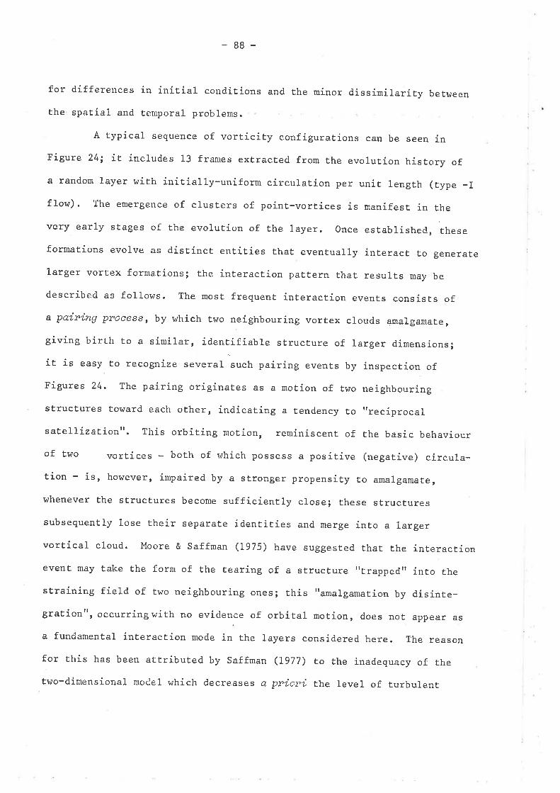
-88-

for dífferences in ínitial conditions and the minor dissimilariËy between

Ehe spaËial and temporal problems.

A typical sequence of vorticity configuraEions can be seen inFigure 24; it includes 13 frames exlracÈed from the evolution history of

a random Layer with initially-uniform circulation per unit length (type -Iflow). The emergence of clusters of point-vortices is manifest in the

very early stages of the evolution of the 1ayer. Once esËablishecl, these

formations evolve as dístínct erÌtities that eventually inÈeract to generate

larger vortex forma.tions; the interacÈion paÈtern that results may be

described as follows. The most frequent interaction events consists ofa paining pnocess, by which two neighbouring vortex clouds amalgamate,

giving birth to a similar, identifiable struct,ure of larger dimensions;

it is easy to recognize several such pairing events by inspection of

Figures 24. The pairing originates as a motion of rwo neighbouring

strucÈures toward each other, indicating a tendency Èo "reciprocalsate11ízationrr. This orbiting motion, reminiscent of the basic behaviour

of two vortices - both of r'¡hich possess a positive (negative) circula-tion - is, however, impairecl by a stronger propensity to amalgamate,

whenever the structures become sufficíently close; these structures

subsequently lose Ëheir separaËe identities and merge into a larger

vortical cloud. Moore & Saffnan (L975) have suggested that Ehe interaction

event may take Èhe form of the tearing of a structure "trappedtr inÈo the

strainíng f ield of tr,ro neighbouring ones; this "amalgamation by disinte-grationt', occurringwith no evidence of orbital motion, does not appear as

a fundamental ínteraction mode in the layers considered here. The reason

for this has been atËribuËed by Saffman (7977) ro the inadequacy of the

two-dimensional model whích decreases a prioni the leve1 of turbulent

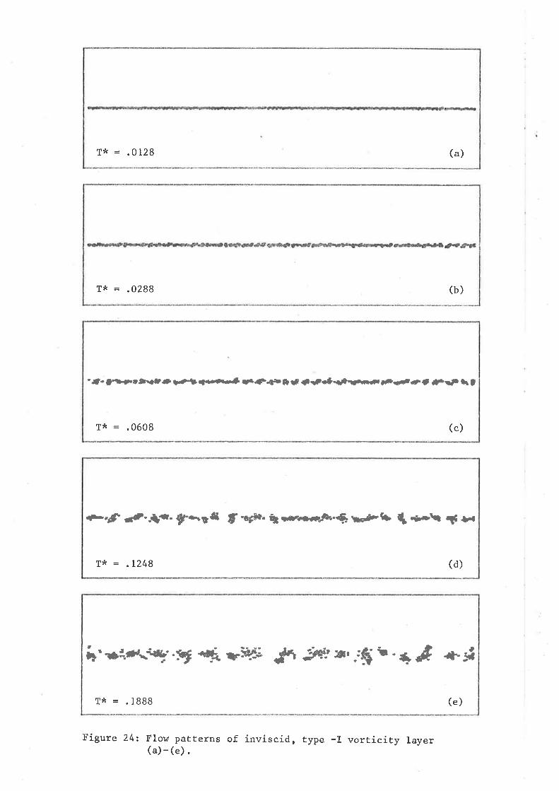
T* = .0128 (a)

T* = .0288 (b)

't- J. -¡.tr.st t-t e{.-ra r.f4** Í {*et.dùç* ÇD€ÇC .Ê !t lì t

T* .0608 (c)

tp.gf rt-.tç. f*t{ f .qCt' Ë rr¡¡a*tÛe-Ç r..g'f ¡[ .¡-tr rÉ +r

T* = .L248 (d)

f'*:.c(+r1'.frf ..{ rV¿ &a æI *,.tS. -+ d {-i¡

T* = .1888 (e)

Figure 24: Flow patterns of(a)-(e).

inviscid, Èype -I vorticicy layer

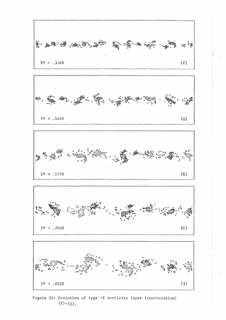
Ë* tru'-g =6¡.ff., # q" --'$..-.* a¿¡# -*yg åЀ

T* = .3168

Figure 24: Evolution of Eype -I vorticity Layer (continuation)(f)_(j).

(f)

Êè Ë #:-.å¡ff.,; '+= .,*#,*-çF'f&S .ç--.:åJÍ

T¡k = .4448 (e)

TEF .Ë.F..rffii..ìi . Riùt-fr.

t .a

'. : '-- #l.',,..

ttt.f

+:Ë t t

T* = .5728 (h)

Ì6. -f;.Eb'.. ._._.'i wË.lt. ¡

T* = .8288 (j)

'$i.-.'¡::,i,..þ t

T* = .7008

.g$'d:'"ï'*6p:t

(

þ.i 'ff)t_

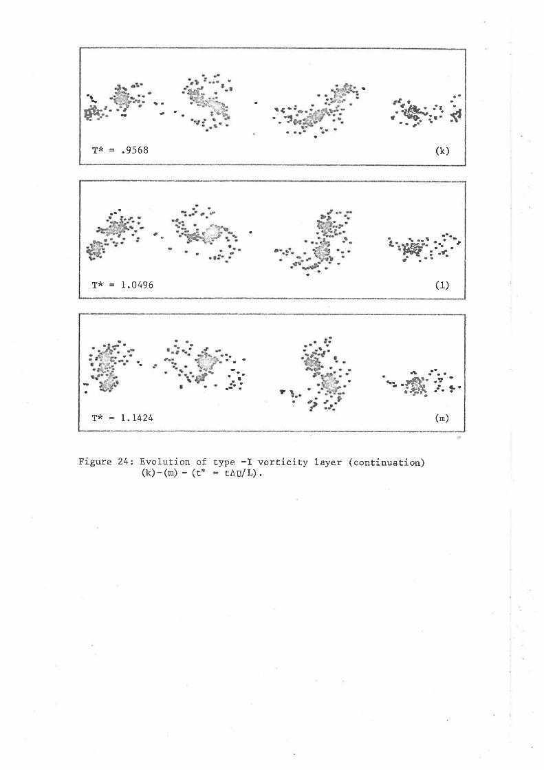
Tx = .9568

ra'..t

I

't

*h; ,'.'@;-;r ¡(k)

a

at¡ t.-r

w: -f

T* = I.0496 (1)

t.I

T* = 1.1424

'¡'lo

(n)

Jt

.€ 3$¿.

?

Figure 24: Evolution of type -I vorticity layer (continuation)(k)-(m) - (r" = tAU/L) .

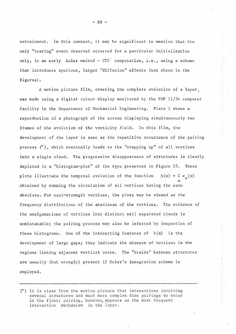
-89-

entrainment. In this conEext, it may be significant to menÈion that the

only t'tearing" evenE observed occurred for a particular initialization

only, in an early Euler method - CTC computatíon, i.e., using a scheme

that introduces spurious, larger rrdiffusionrr effects (not shown in the

figures) .

A motion picture film, covering the complete evolution of a layer,

was made using a digital colour display monitored by the PDP 11/34 compuÈer

facility in the DepartmenE of Mechanical Engineering. Plate 1 shows a

reproducÈion of a photograph of Ehe screen displaying simultaneously two

frames of the evolution of the vorticity field. In this film, the

development of the layer is seen as the repetitive occurrence of the pairing

process (* ) , which eventually leads to the t'wrapping up" of all vortices

into a single cloud. The progressive disappearance of structures is clearly

depicted in a "histogram-p1ot" of the type presented in Figure 25. These

plots illustrate the temporal evolution of the funcÈion h(x) = X ro(x)cl

obtained by summing the circulation of all vortices having the same

abscissa. For equi-strength vortices, the plots may be viewed as the

frequency disEributions of the abscissae of the vortices. The evidence of

the amalgamations of vortices inÈo disEincE well separated clouds is

unmistakable; the paíring process may also be inferred by inspection of

these hisEograms. One of Èhe interesting feaEures of h(x) is the

developmenÈ of large gaps; they indicate the absence of vortices in Èhe

regions linking adjacent vortical cores. The "braidst' between structures

are usually (but w::ongly) present if Eulerrs integration scheme is

employed.

It is clear from the motion pieture that interactions involvingseveral structures and much more complex than pairings do occurin the flows; pairing, however, appears as the mosÈ frequentinteraction mechanism in the layer,

(*)

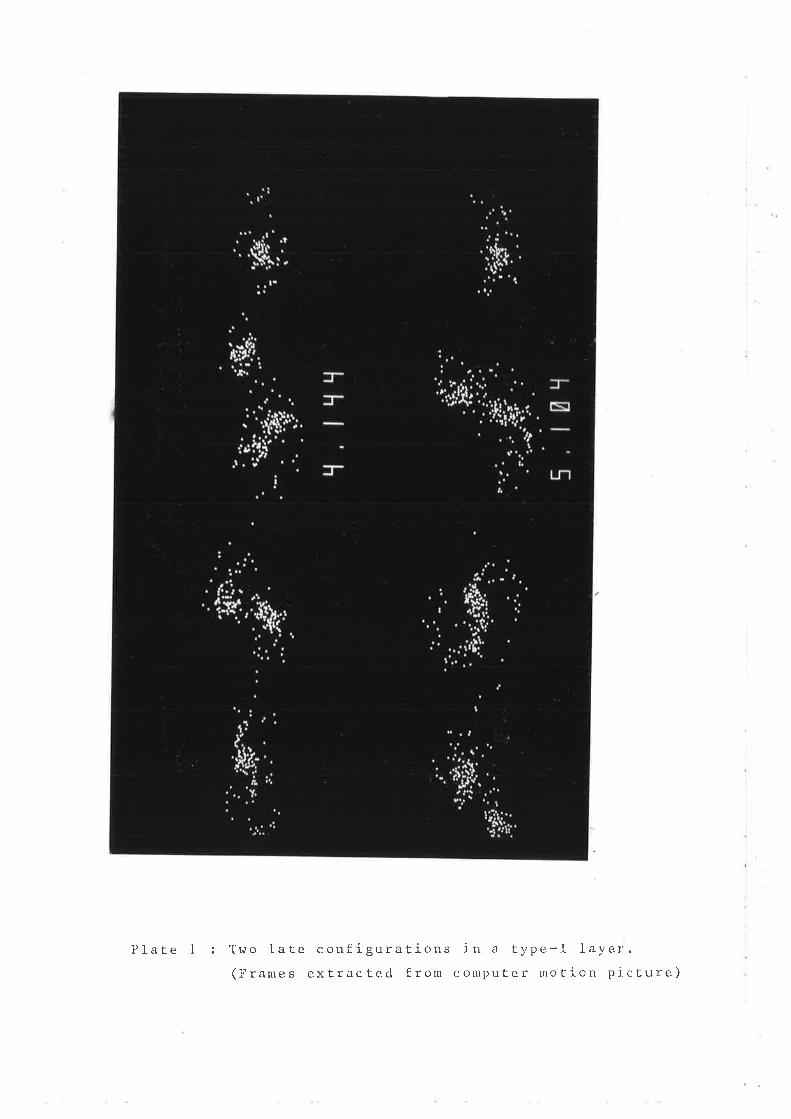
PIace I : Two late coufiguraEions in a type-I layer.(!-ranes extract.ed fron conputer motion pí.ctu::e)

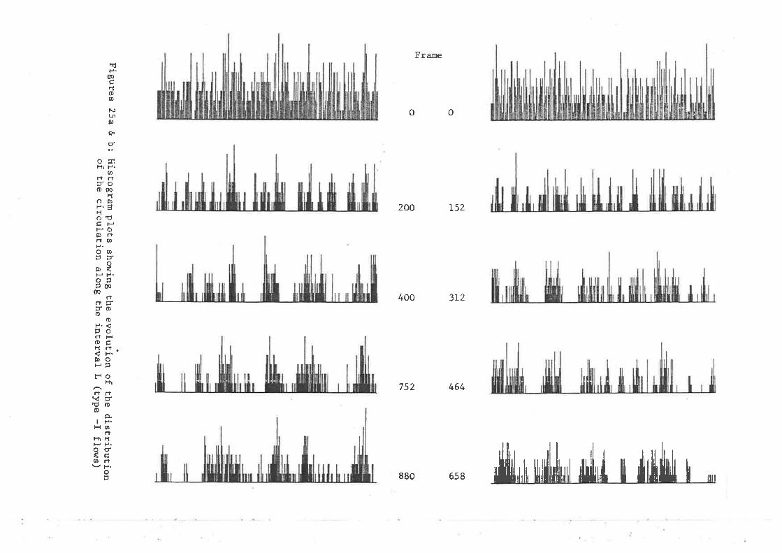
-:-........l

-J--_.-|=

=E

---Iã

--=!

-=-!l¡5<--

________---:=E

--

- -=-

-=

@tn\oo@æ

Nrôr\oo.t

ooN

\f\o\1NF

-{

cîNLrlF

.loo

oá(Il¡rÍ¡{

Fígures 25a &

b: HisÈ

ogram plots show

ing Èhe evolutio¡ of the distribution

of the circulation along the interval L (type -I flow

s)

90

On the basis of the above discussion, the model appears to

accuraEely predict qualitative aspects of Èhe flow. Quantitative

comparison between the model estimateò and experimental evidence is Ehe

object of the following paragraphs, beginning with the growth histories

of the sample flows.

fÍL4.2 The growth of the layers

TII.4,2.L Theoretical background

The self-preservation hypothesis, applied to inhomogeneous spatiaL

mixing layers, asserts that, at sufficiently large values of R"* = xUr/v,

the streamwise velocíty distribution U(y) and the density field p (y)

exhibit mean profiles of the form

u(n; r,s)

I g. ro](n; r, s)

Uqp

P1

F

Fp

where \=y/(x-x.)r = tJr/tJ,

and s = pz/pL

is the similarity variable,

is the velocity ratio,

is the density ratio.

Layers r¿ith mean velocity (density) profiles that scale like [3.f0] must

grow linearly as they develop downsÈream. DenoÈing by ôrr(x) (Oo{")) .t

estimate of the layer thíckness based on Èhe velocity (density) profile,

one predicts the dependence

(x-x.) Cr, (r,s)

oo( x) c

ô (x)u

(x-x.)p

(r, s) ,

[ 3.11]

-91 -

where C.. and C^ are consËants for any fixed choice of values of r and s.upExamination of the layer spreading rate provides therefore a simple means

of EesEing the relevance of the self-preservation arguments (note that a

linear spreading is a necessary but noÈ sufficient condition for self-

preservaËion to be established). Knowledge of the functional dependence of

the spreading raËes C (rrs) on the velocity and density ratios relies

essentially on experimenEal investigation. The spreadíng raÈe function

Cr(r) for the vorticity thickness (*) of homogeneous layers (s=1) has

been determined in various experimental situations. Presently available

data suggest a possible linear dependence of Cr(r) on the velocity

difference parameter I = 2AU/U"; at small values of À, Ehe Abramovich-

Sabín relaÈionship appears to hold:

(r) [ffi)*, I 3.L21c(¡)

where K.. is a constant. Data are well represented, at small À, withu)

K. = O.181. Alternative functional forms of the spreading function are(t)

discussed at length by Brown & Roshko (1974).

The spreading of spatial layers is perceived as a growth with time

in Èhe corresponding Eemporal problems. Dimensional considerations dictate

that temporal layers gror¡/ according to the law

ô (r) = (r-r.) AU KT t3.131uJ- - uJ

T Using the Galilean transformation (t-t.)

= lÁ(uL+uz) Yields Lhe equation

where K

(x-x.) /U

is a constant.u)

c vrith Uc

ult

(*) the vorticity Èhickness ô.. is defined as ô,, = lLtJ/sign being selected accordTng to that of the*velocitygradient.

(Pr)"*'the

-92-

6üJ

t 3.141X-Xo

which is identified as the Abrarnovich-Sabin relationship. The expected

value for KÏ is therefore KT = K^/2 È .09. NoEe rhat Ëhis Galilean

transformatíon is only appropriate for ¡¡/Ult smal1.

The growth of the computed layers was determined from the change

with time of the vorticity thickness; Èhis was preferred to the visual

thickness whose determination appeared largely too subjective. The

vorticiCy thickness was determined from the mean velocity profile, fitted

with a high-order polynomial over iÈs central portion (to avoid the long

flat tails of the profile far from the layer). Typícally, average values

v¡ere computed over 75 stations uniforrnly distributed over the interval

length; 7Eh-order polynomials wire fitted to averaged dala over an interval

in the Eransverse direction equal to 1207. of the visual layer thickness.

This procedure was found to yield smooth velocity profiles and results

faftIy insensit,ive to changes in the parameters. Occasionally, for very

thin layers, some uncertainty could noË be avoíded in the estimation of ôr.

The thickness may also be determined from the probability distribution,

p(y), of the number of vortices, using the relationship

( 1-r )zI+r KTüJ

ô [ 3. is]OJ

Expression [ 3.15] may be established as follows. Consider a layer of

period L, discretized by equi-strengEh point-vortices. Be n(y)dy the

number of vortices locaÈed in the strip (y,y+dy); they carry a circulaÈion

y(y) = yn(y)dy, where y is the individual vortex strength. Compute Ehe

circulaÈion around a strip of height dy which covers the cyclic interval

L. Clearly, one has V(y) = - | # Ut

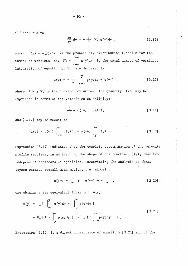
and rearranging:

u(y)

where I=yNVrs

expressed in terms

and [ 3.17] may be recasË as

ðydy - + NV p(y)dyàu

-93-

rL

where p(y) = n(y)/NV is the probability distribution function for the

number of vortices, and NV = f*- rr(y)dy is the total number of vortices.l_@

InÈegration of equation [3.16] yields directly

[ 3. 16]

[ 3. 17]

[ 3.18]

[ 3.le]

[ 3.20]

[ 3.2i]

Jl- p(y)dy + u(--)

Ehe total circulatíon. The quantity f/L may be

of the velocities aE infinity:

T

i = .t(-*) - u(+-),

u(y) = u(+-¡ p (y) dy + u (-æ)

one obtains Èhree equivalenE forms for u(y):

u(y) U II p(y)dy - p(v)dv l

Jl_ I p (v) ¿v.Jy

Expression [3.19] indicates that the complete determination of the velocity

profile requires, in addition to the shape of the funcÈion p(y), thaE two

independent constants be specified. Restrícting the analysis to shear

layers lrriËhout overal l mean mot ion , i . e . choos ing

u(+*¡ =U* ; u(--) --U_

@ Jl-@

f]_' (y)dy - 1 Iv

= fJ lI-2 p(y)dy I = U- [2

Expression [3.f5] is a direcE consequence of equations [ 3.2L1 and of the

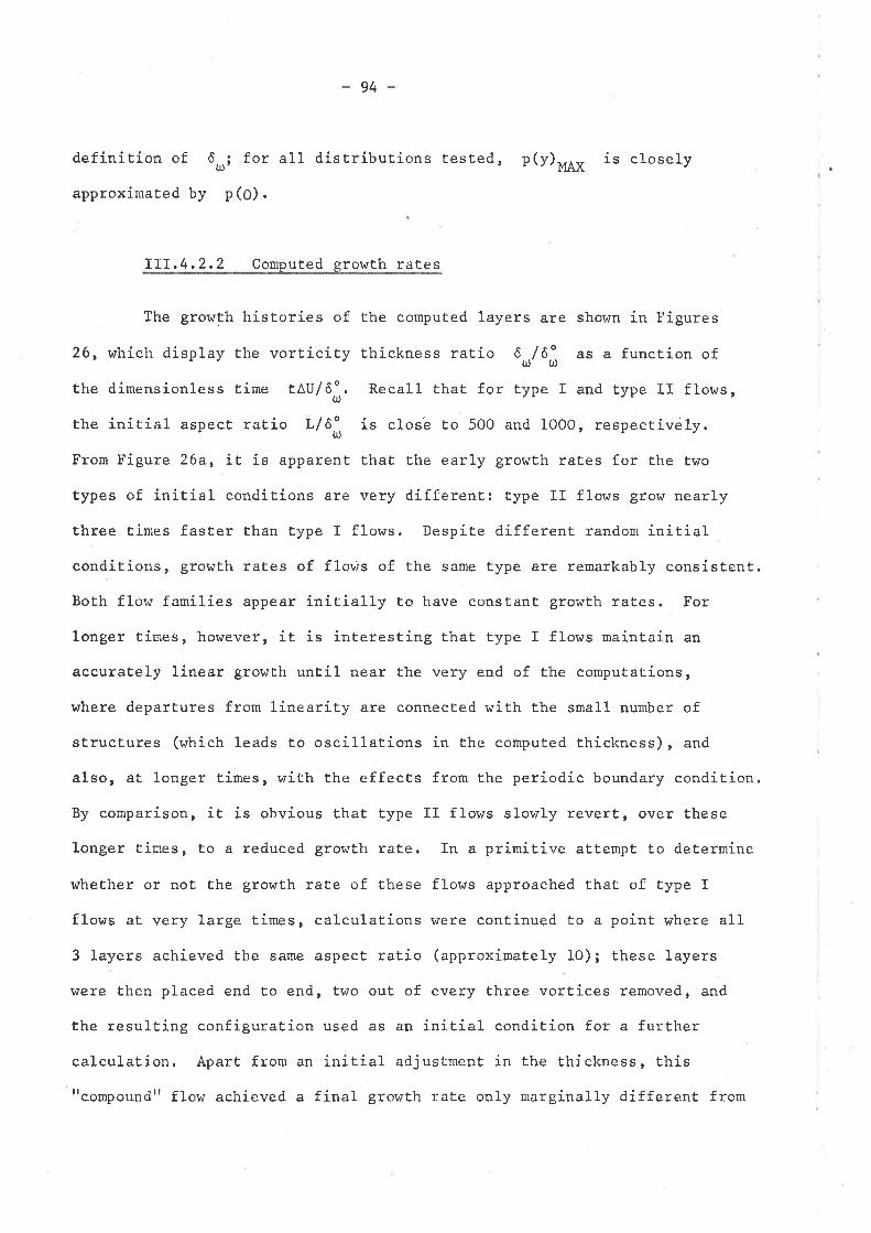
94

definition of 6ri for all distributions tested, n(f)"* is closely

approximated by p (O) .

TIT,4.2,2 Computed growth raÈes

The growËh hisEories of the computed layers are shown in Figures

26, which display Èhe vorticíty thickness ratio 6u,/6; as a function of

the dimensionless Ëime t¡U/ôå. Recall thaE for type I and type II f1ows,

the initial aspecÈ ratio L/6; is closb to 5OO and 1OOO, respectivály.

From Figure 26a, it is apparent that the early growth rates for the two

Ëypes of initial conditions are very differenE: type II flows grow nearly

three times faster than type I florss. Despite different random initíal

conditions, growÈh raÈes of floûs of the same type are remarkably consistent.

Both flor¡ families appear initially to have constant growth rates. For

longer times, however, it is interesting that type I flows maintain an

accuraÈely linear growth until near the very end of the computations,

where departures from linearity are connected with the small number of

struct,ures (which leads to oscillations ín the computed thickness), and

also, at longer times, wiËh the effects from the periodic boundary condition.

By comparison, it is obvious that type II flows slowly revert, over these

l-onger times, to a reduced gro\,rth rate. In a prímitive attempt to determine

whether or not the growth rate of these flows approached that of type I

flows at very large times, calculations \,/ere continued to a point where all

3 layers achieved the same aspecÈ ratio (approximately 10) ¡ these layers

were then placed end to end, Ewo out of every Èhree vortices removed, and

the resulting configuration used as an initial condiEion for a further

calculation. Apart from an inítial adjustment in the thickness, thist'compound" flow achi-eved a final growth rate only marginally different from

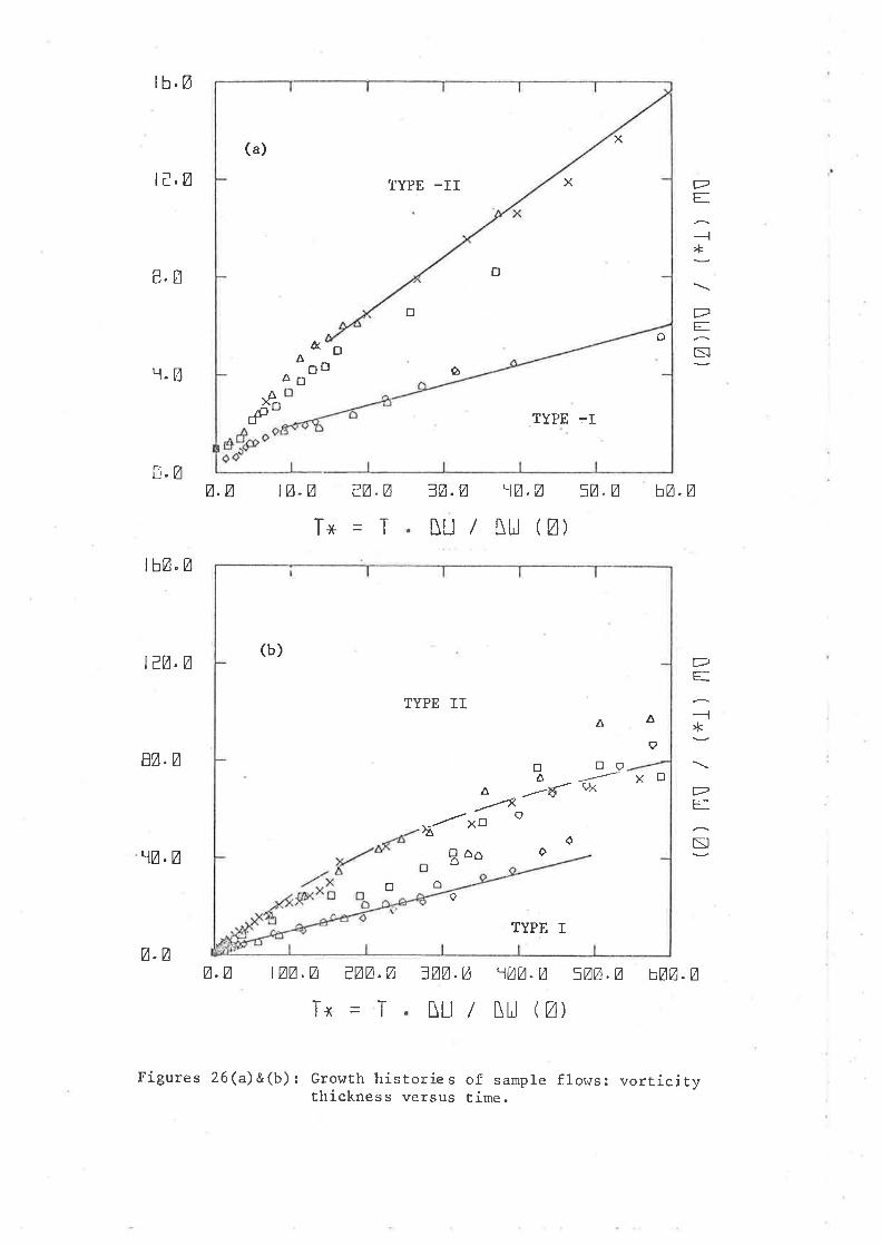
lb.Ø

r¿.2

B.I]

r.Ø

z.Ø

lÉØ. Ø

t¿Ø. Ø

EØ.Ø

!'Ø.Ø

Ø.Ø

Ø.Ø

Ø.Ø

3Ø. Ø

[u/

=ØØ. Ø

[u/

PE

---{

L

PES¡

IØ-Ø ?Ø.Ø

fx=T

tØØ.Ø eØØ.Ø

Tx=T

rØ.Ø 5Ø.Ø

[u (Ø)

hØ. Ø

1ØØ.Ø =ØØ.Ø

bØØ.Ø

ùrJ (Ø)

E

*

E

5

Figures 26(a)&(b): Growth histories of sampre fl-ows: vorticitythickness versus Èime.

(a)

TYPE -II

Âg

TYPE :I

X

X

D

tr

ôo

^ à

i"&gD

(b)

TYPE II

oA

Boo

TYPE I

AA

Eççx -..¿4

/-t4xDQtL

oo

ôtra

I

Xtr

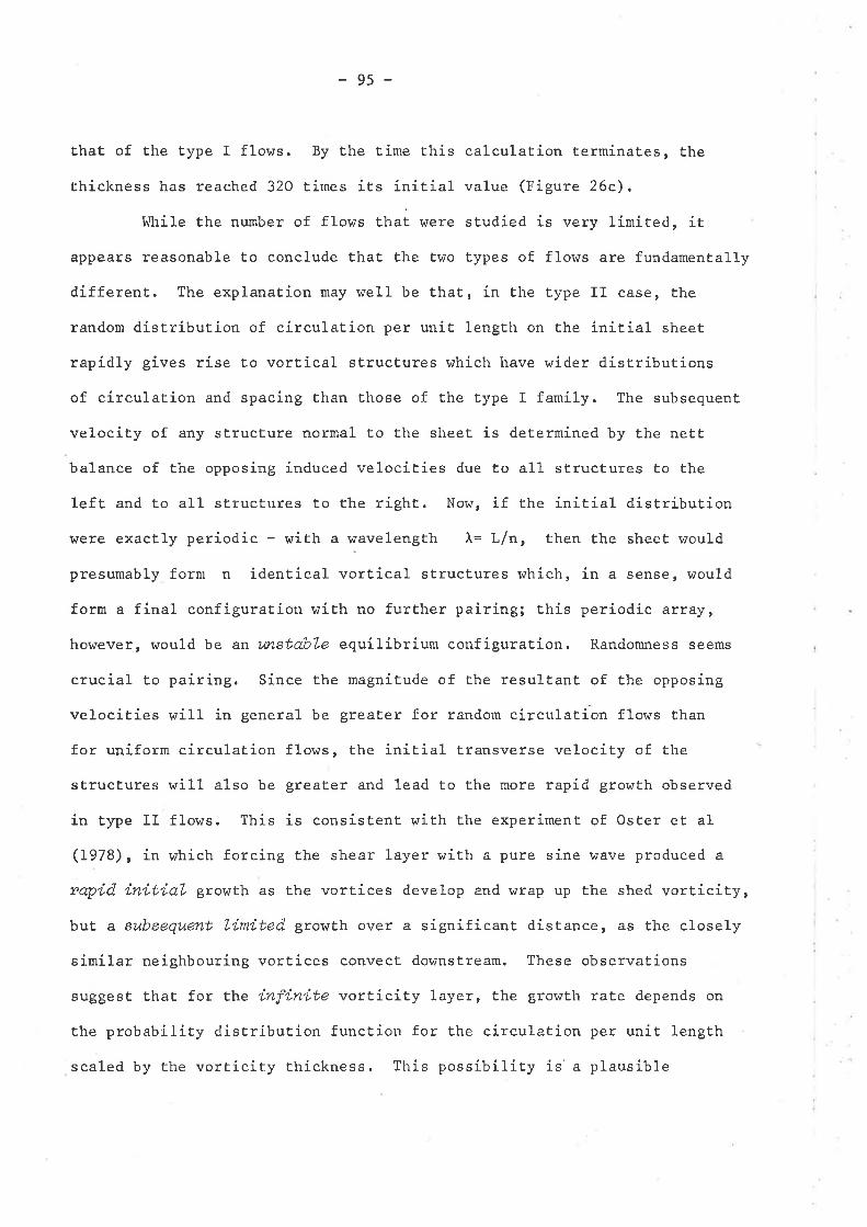
-95-

ËhaE of the type I flows. By the time this calculation termínates, the

thickness has reached 320 Èimes its initial value (Figure 26c).

hlhile the number of flows thai were studied is very limited, it

appears reasonable to conclude that the Èwo types of flows are fundamentally

different. The explanaÈion may well be that, in the type II case, the

random distribution of circulaEion per unit length on the initial sheet

rapidly gives rise Eo vortical structures which have wider distributions

of circulaEion and spacing than those of the type I family. The subsequent

velocity of any structure normal to the sheet is determined by the neÈÈ

balance of the opposing induced velocities due to all structures to Èhe

left and to all structures to the right. Now, if rhe inirial distribution

!'rere exactly periodic - with a wavelength À= L/n, Èhen the sheet would

presumably form n identical vortical structures which, in a sense, would

form a final configuration with no further pairing; this periodic axray,

however, would be an mstabLe equilibrium configuration. Randomness seems

crucial ro pairing. Since the magniÈude of the resultant of the opposing

velocities will in general be greater for random circulatíon flows than

for uniform circulation flows, the initial transverse velocity of the

strucËures will also be greater and lead Eo the more rapid growth observed

in type II flows. This is consistent v/ith the experiment of Oster et al

(1978), in which foreing the shear layer v¡ith a pure sine wave produced a

rapid initial grovrth as Ehe vortices develop and wrap up Èhe shecl vorticity,

but a subsequent Limùted growth over a sígnificant distance, as the closely

similar neighbouring vortices convect downstream. These observations

suggest that for the ínfinite vortícit,y layer, the growÈh rate depends on

the probability distribution funcÈion for Ehe circulation per unit length

scaled by the vorticity thickness. This possibility is a plausible

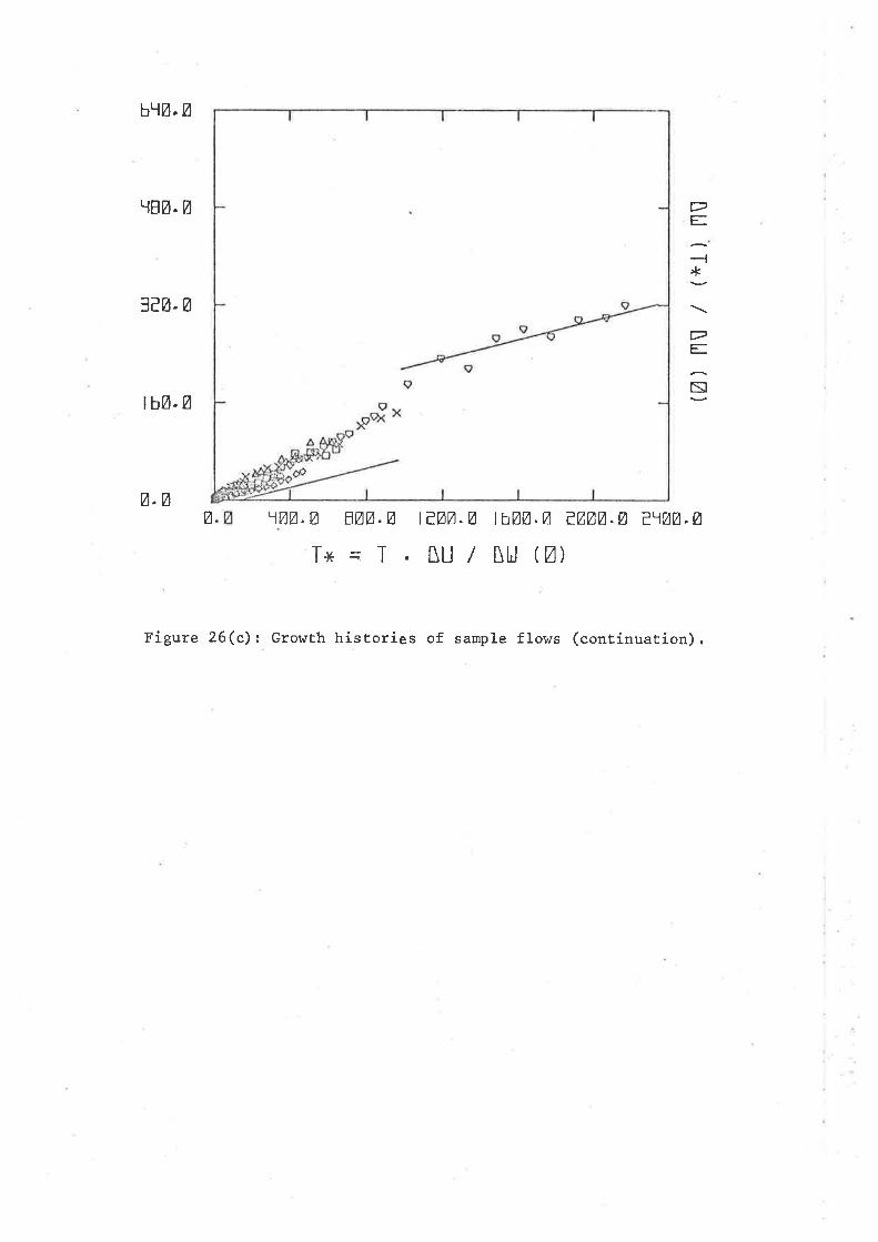
bLlø. Ø

TBØ. ø

3¿ø.ø

tbØ. Ø

Ø.ø

PE

-l*

PE

ñ

ø 1øØ.Ø

fxBØØ. Ø

=Tt¿ØØ. Ø

ßu/lhØØ.Ø ¿ØØØ.Ø erøØ.Ø

[u (Ø)

Figure 26(c): Gror,¡Èh histories of sample flor,¡s (continuation).

-96-

explanaEion for Ehe behaviour of type II flows. For the infinite sheet,

dimensional analysis predicts that the layer should grow linearly; that it

does not for type I,I flows presumably'reflects the significance of the

periodiciËy in L. For these flows, Èhe circulat,ion per uniE length will

tend Eo become more uniform - ôûr/L increasing - as the initially random

strength, small-sca1e st.ructures combine¡ a grov¡th rate which decreases

Èowards that of Èype I flows may Èhen be expected.

The present results are consistent \,rith the wide variation in the

experímentally found growth rates of mixing layers, and particularly with

the known sensitivity to a trippíng device. Differences in growth rate as

large as those between the tr¿o classes of flows studied here have not been

found experimenEally; yet, a trip will tend to introduce a randomness in

the circulation about any small circuit near the splitter plate. This

randomness - Èhough not as large as thaË present. in the calculaEions - may

be responsible for the dramatic ehange in the spreading rate of tripped

layers. In Eype I flows, the randomness in circulation is introduced

ttlocallytt, i.e. on the scale of the spacing between two vortices; on a

scale of several times the initial vorticity thickness, the circulation per

unit lengrh is uniform, and the randomness looks rather like a random

displacement of the vorticity layer. This situation, one expects, models

more closely the usual spliÈter plaEe condition aÈ high Reynolds number.

It ís interesÈing Èo note that the asymptotic growth rate 6r/AU of Ehe

type I flor¿s is close to.O8, over a very large increase of thicknesq

(Figure 26b). This is to be compared v¡ith the value .09 inferred from

experimental data and reporEed in the preceding section.

A predíction which would fo1low from Ehese considerations is that

a broad-band random fluctuatíon ín time (not space) of the free-stream

97-

velocity - for example, Ul = Ur(t) - would have a significant effect on

the spreading rate of spatial layers. This may have interesting implications

when considering Èhe possible connection with the effects of mass fl-ux

variations in jets.

hlhatever the explanaEion for the behaviour of the calculated gror+th

histories, it is clear that different types of inítial conditions have a

persistent effect, in these effectively inviscid flows, over time inEervals

that appear surprisíngly large. A measure of time in the spatial turbulenE

mixing layer, proposed by Dimotakis & Bror,øn (L976), scales with the number

of amalgamalion (pairing) events undergone by the sEructures as they

evolve downsLream. The number of interactions m(x) that take place over

a downstream distance x is given by m(x) - 1o12(x/9,"), where !-o is the

wavelength of the original disturbance. This estimate is based on Ëhe

assumpt,íon Èhat each pairing inÈeraction doubles the spacing between the

sËructures. According to this measure, 5 or 6 amalgamatíons have taken

place during Ëhe history of the calculated flows; this is of ínEerest if

one noÈes that the same number of interacÈions have occurred by the tirne

structures reach the farthest measuring st.ation in t.he Dimotakis & Brown

experiment; in most laboratory configurations, this number does not exceed

10 over the full lengËh of Ëhe apparatus.

III.4.3 Correlation analysis of the velocity fieta

The evidence drawn from the analysis of the grovith historie.s of the

computed flows suggests that Ehe large scale structure of random vortieity

layers may evolve asArtptoticalLy Eowards a universal state, characterízed

by a unique, constant growth rate. This tendency is in agreement $rith

conclusions drawn from dimensional arguments applied t.o the infinite vortex

98-

sheet. IE is important to collect, additional information about the possible

self-simílar structure of these layers; it is also interesting Èo compare

the characteristics of the strucEures'that arise in two-dimensional

compuËations with these observed in the turbulent mixing layer. This dual

purpose may be fulfilled through the analysis of the correlation functions

of the fluctuating velocity field, as described below.

The asyrnptotic evolution of mixing layers Ëowards a fully three-

dimensíonaL selÍ.-preserving turbulent structure has been reported by various

authors and is substantiated by a large amounÈ of experimental daÈa

(Chandrsuda et, al, 197S). The uniqueness of this asymptotic sÈate appears,

however, questionable in view of the evidence thaË an apparently distinct,

essentialLy tuo-dimensionaL self-preserving state may also develop in

turbulent mixing layers (¡imotakis & Brown , Lg76). The possible connection

between the latter type of flow evolution and the behaviour of the present

numerical flows is without doubE an interesting one.

In thei:: experimental investigation of a mixing layer in water,

Dimotakis and Brovm examine the behaviour of the autocorrelation function

of the streamwise velocity fluetuations in terms of simil.arity properties

and initial-conditions dependence. They report that the autocorrelation

funct,ions R r, (t) = < u'(t) u'(t + t) > exhibit the fundamental periodici-

Èy that would be expected from similarity arguments. Their results inclicate

that the ratio ,o/r" , where a" represenÈs the downstream convect,ion1

Èime of Ehe structure (r" X - xo / i Q, + U2)), is effectively constant

for all xrU, and Urr for a given velocity raEio r = lJr/lJr. The average

spacing between Èhe structures inferred from their data is found to fall

in Ehe range 3.1 . I/ ôo < 5., ô, being the vorÈícity thickness of

the layer.

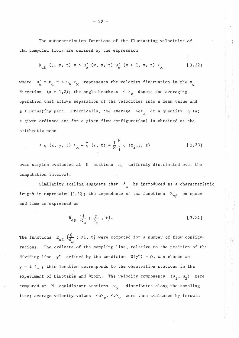
-99-

The autocorrelation functions of the fluctuating velocities of

the computed flows are defined by the expression

u (t; v, t) -. ná (x, y, t) uo (x+ t, Y, t)R

where rí = ro - . to t* represents the velocity fluctuation in Ëhe xo

direction (a = 1r2); the angle brackets . t* denote the averaging

operatíon thaE allovùs separation of the velocities inÈo a mean vaLue and

a fluctuating parÈ. Practical-1y, the average .gt* of a quanÈity q (at

a given ordinate and for a given flow configuration) is obtained as the

arithmetic mean

[ 3.23]

0

over samples evaluated at N sÈatíons x

computation interval.

Similarity scaling suggests that

length in expression [:.22; the dependence of

and time ís expressed as

l,3 , zz7x

. uniformly disÈributed over the

6 be introduced as a characteristrc

the functíons on sPace

< q (x, y, r)'*= ã (y, È) =+i q (xi,y, t)1

(,tJ

Roß

Rqß r) . I g.z+l

The functions Roß (t t tl, t) were computed for a number of flow configu-

rations. The ordinaÈe of the sampling line, relative to the position of the

dividing line y* defined by Èhe condition U(y*) = O, Ì{as chosen as

y = * ô, i this location corresponds to the observation stations in the

experiment of Dimotakis and Brown. The velocity componentt (ul , u2) r¡rere

computed at N equidistant stations *o distributed along the sampling

line; average velocity values .rt*, .tt* were then evaluated by formula

vô

UJ

(E\ô

ü)

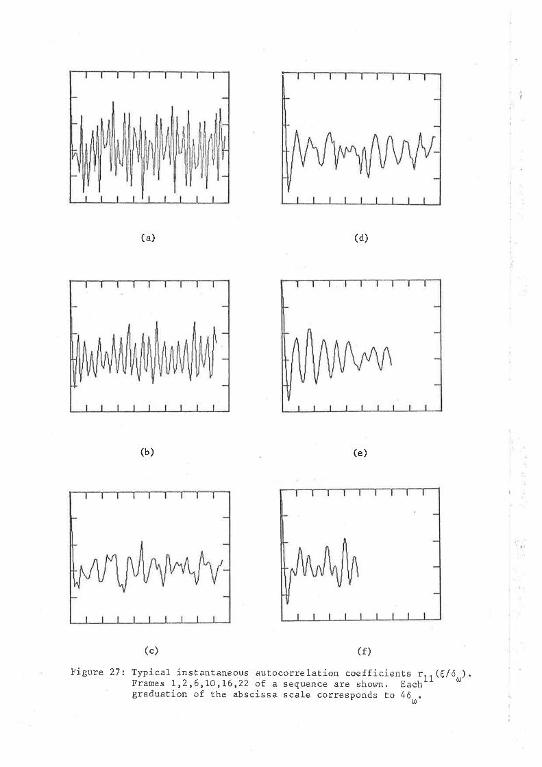
(a) (d)

(b) (e)

(c) (r)

Figure 27: Typí.cal insLantaneous autocorrelation coefficients rF::ames 1-1216110r16 r22 of a sequence are shovrn. Eachgraduation of the abscissa scale corresponds to 4ôr.

r1 (E/6(¡) .

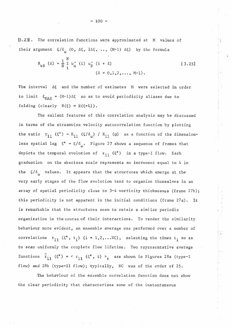
-100-

13,231. The correlation functions r^rere approximated at M values of

their argument t/ôo (0, 46, 2AE, .., (M-1) At) by the formula

Roß (r,) (i) (i+t)

(1, = 0rL12r..., M-1).

[ 3.2s]

The interval At and Èhe number of estimates M were selected in order

to limit tì.,fAX = (If-l)^t so as to avoid periodicity aliases due to

folding (clearly R(E) = R(t+L) ) .

The salíent features of this correlation analysis may be discussed

in terms of the sÈreamr¡ise velocity autocorrelation funetion by plotting

Èhe ratio tll (g*) = Rll (E/ôo) / *r, (o) as a function of the dimension-

less spatial lag t* = 6/ôtr. Figure 27 shows a sequence of frames Ëhat

depicts the temporal evolution of r1l (t*) in a type-I flow. Each

graduation on the abscissa scale represents an incremenE equal to 4 in

the 6/ô,¡ values. It appears that Èhe structures which emerge at the

very early stages of the flow evolution tend to organíze themselves in an

array of spatial periodicity close to 3-4 vorticity thicknesses (frame. 27b);

this periodicity is noÈ apparent in the inítial conditions (frame 27 a) , IE

ís remarkable that the structures seem to retain a similar periodic

organízation in thecourse of their interactions. To render the similarity

behaviour more evidenÈ, an ensemble average vras performed over a number of

correlations r11 (t*, ai) _(i = 1,2,...NC), selecting the rimes ti so as

to scan uniformly the complet.e flow lifetime. Two representative average

funct,ions tll (t*) =. tll (t*, t) tt are shown ín Figures 28a (type-I

flow) and 2Bb (type-Il flow); typically, NC r¡as of Èhe order of 25.

The behaviour of the ensemble correlation function does not show

the clear periodiciÈy that characterízes some of the instantaneous

u-NI.

--¿uNoI Ê

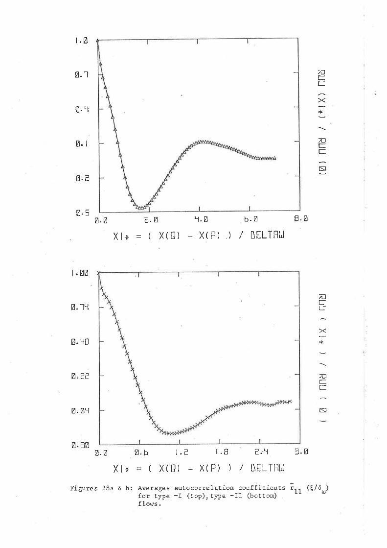
l.Ø

Ø.1

Ø. t]

ø, 1

Ø.e

Ø-5

l.ØØ

Ø. lr

Ø. TB

Ø"?¿

Ø.Ø1

ø.3Ø

Ø.Ø

-lrJ

E=><

t<

nEE

N

e.ø

Xlx ( X(E)

1.Ø

X(P) )

b.Ø

i ttLlflu8.Ø

3.ø

nrL:

X>k

Tff

S¡

Ø.Ø z.b

Xl+

Figures 28a & b: Averages autocorrelation coefficiela" iff (E/ôr)for type -I (top), Eype -II (bottom)flows.

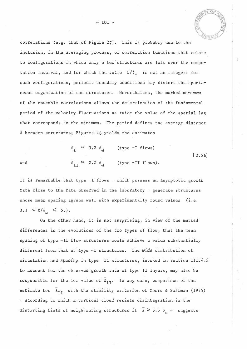
-101-

correlations (e.g. that of Figure 27). This is probably due to the

inclusion, in the averaging process, of correlation functions that relate

to configurations in which only a few'structures are lefL over the compu-

tation inËerval, and for which the ratio l,/6t: is not an integer: for

such configurations, períodic boundary conditions may distort the sponEa-

neous organizalion of the structures. Nevertheless, the marked minimum

of the ensemble correlations allor¡s Ehe determination of Èhe fundamental

period of the velocity fluctuations as twice Ëhe value of the spatial 1ag

thaÈ corresponds to the minimun. The period defines the average dístarice

I betwe"r, structures; Figures 28 yields the estimaÈes

TI 3.2 ô (type -I flovrs)üJ

I 3.261

and 2.0 ô.d (type -II flows).

It is remarkable that Èype -I flows - which possess an asymptotic growth

rate close to the rate observed in Ehe laboratory - generate structures

whose mean spacing agrees well with experimentally found values (i.e.

3.1 <¿/ô < s.).u)

On the oEher hand, it is not surprising, in view of the marked

differences in the evolutions of the t\^/o types of flow, that the mean

spacing of type -II flow structures would achieve a value subsÈanEially

different from that of type -I structures. Tlne uide distribuEion of

circulation and spacing in Ëype LI structures, invoked in Section IIL4,2

to account for the observed growth rat.e of type II layersr may also be

responsible for the low value of lrr. In any case, comparison of the

estimate for I' r^rith the stability criterion of Moore & Saffman (Qg75)

- according to r¡hich a vortical cloud resists disintegration in the

¿ > s.5 ô(¡)

Lrr o

disÈorting field of neighbouríng structures if sugges t s

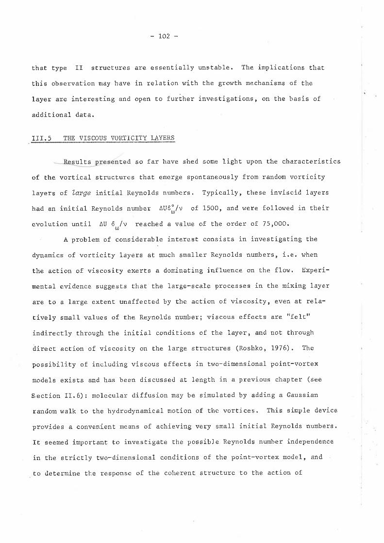
-LOz-

thaË type II structures are essentially unstable. The implications that

this observation may have in relation with the growth mechanisms of the

layer are interesEing and open to further investigations, on the basis of

additional data.

III.5 THE VISCOUS VORTICITY LAYERS

ult s ted so far have shed some light upon the characteristics

of the vortícal sEructures that emerge spontaneously from random vorticiÈy

layers of Latge initial Reynolds numbers. Typically, these inviscid layers

had an initial Reynolds number nUôiiv of 1500, and were followed in their

evoluÈion until ÂU ôr/v reached a value of the order of. 751000.

A problem of considerable interest consisËs in investigating the

dynamics of vorticity layers at much smaller Reynolds numbers, i.e. when

the acÈion of viscosity exerÈs a dominatíng influence on the flow. Experi-

mental evidence suggests that the large-scale processes in the mixing layer

are Eo a large extent unaffected by Ehe action of viscosity, even at rela-

tively small values of the Reynolds number; viscous effecEs are t'felt"

indirectly through the initial conditions of the layer, and noÈ through

direct action of viscosity on Ehe large structures (Roshko, L976). The

possibility of including viscous effects in tr¡o-dimensional point-vortex

models exists and has been discussed at length in a previous chapEer (see

S.ection II.6) : molecular diffusion may be simulated by adding a Gaussian

random walk to the hydrodynamical moÈion of the vortices. This simple device

provides a convenient means of achieving very small initial Reynolds numbers.

It seemed important to invesÈigate the possible Reynolds number independence

in the strictly two-dimensional conditions of the point-vortex mode1, and

to determine the response of the coherent strucEure to the action of

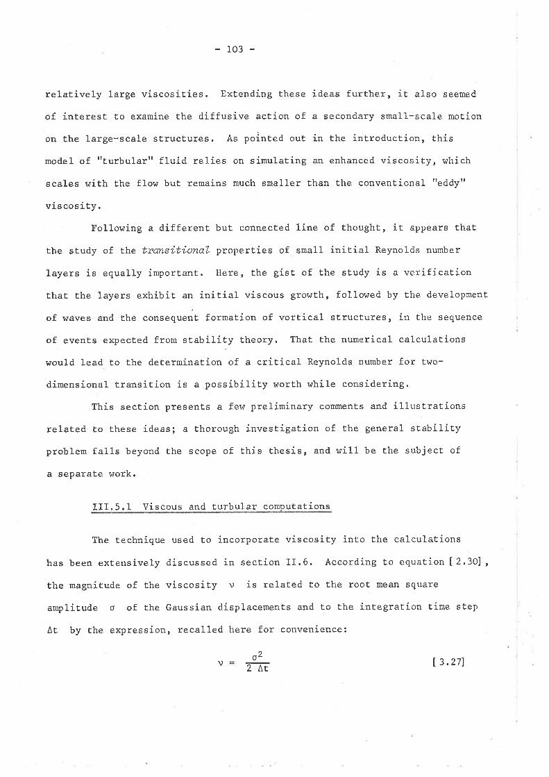
-103-

relaËively large viscosities. Extending these ideas further, it also seemed

of interest to examine Ëhe diffusive action of a secondary small-scale moEion

on the large-scale structures, As pointed out in the introduction, this

model ofttturbularttfluid relies on símulating an enhanced viscosity, which

scales with the flow but remains much smaller than the conventional t'eddy"

vis cos ity.

Following a different buL connected line of thought, it appears ÈhaË

the study of the trcnsitional properties of small initial Reynolds number

layers is equally import,ant. Here, Èhe gist of the sÈudy is a verification

thaË the layers exhibit an initial viscous gror,ath, followed by the development

of waves and the "orrr"q,r"rt formation of vorÈical strucLrrres, in the sequence

of events expected from stability theory. That the numerical calculations

would lead to Èhe deËermination of a crit,ical Reynolds number for two-

dimensional transition is a possibility worth while considering.

This sectíon presents a few preliminary comments and íllustrations

related to these ideas; a thorough investigaÈion of the general stability

problem faIls beyond the scope of this thesis, and will be the subject of

a separate work.

III.5 . 1 Viscous and turbular computations

The Èechníque used to incorporate viscosity into Ehe calculatíons

has been extensívely discussed in secËion II.6. According to equation 1.2.30] ,

the magniEude of the viscosity v is related to the rooË mean square

amplitude o of the Gaussian displacements and to the integration time step

AË by the expression, recalled here for convenience:

o2mîv Í 3.271

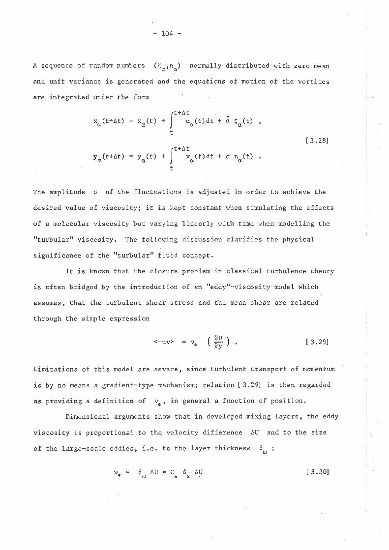
104 -

A sequence of random numbers (Çarna) normally distributed with zero mean

and unit variance is generated and the equations of motion of the vortíces

are integrated under the form

Arq, uo(r)¿r + å çc(r)

[ 3.28]

y0 (E+At) +

The amplitude o of the flucEuations ís adjusted in order to achieve the

desired value of viscosity; it is kepÈ consÈant v¡hen simulating the effects

of a molecular viscosity but varying linearly with time when modelling the

r'Ëurbular" viscosiÈy. The following discussion clarifies the physical

significance of the rrturbular" ìfr'rio concept.

It is knor.¡n that the closure problem in classical turbulence the-ory

is often bridged by the introductíon of an "eddy"-viscosity model which

assumes, that the turbulent shear str:ess and the mean shear ate relaÈed

through the simple expression

(-uv) v* l3.zel

Limitations of this model are severe, since turbulent transport of momentum

is by no means a gradient-Ëype mechanism; relation [3.29] ís then regarded

as providing a definition of vr., in general a function of position.

Dimensional arguments shor+ that in developed mixing layers, the eddy

víscosity is proportional to the velociÈy difference AU and to the size

of the large-scale eddies, i.e. to the Layer Ehickness ô, :

v* c ô, AU = C* ðu, AU [3.30]

f'.È

+x,, (t)(r+Ar)x

y0(t)rt+At

.J "r(r)dr+o¡o(t)t

AU

ãt )t

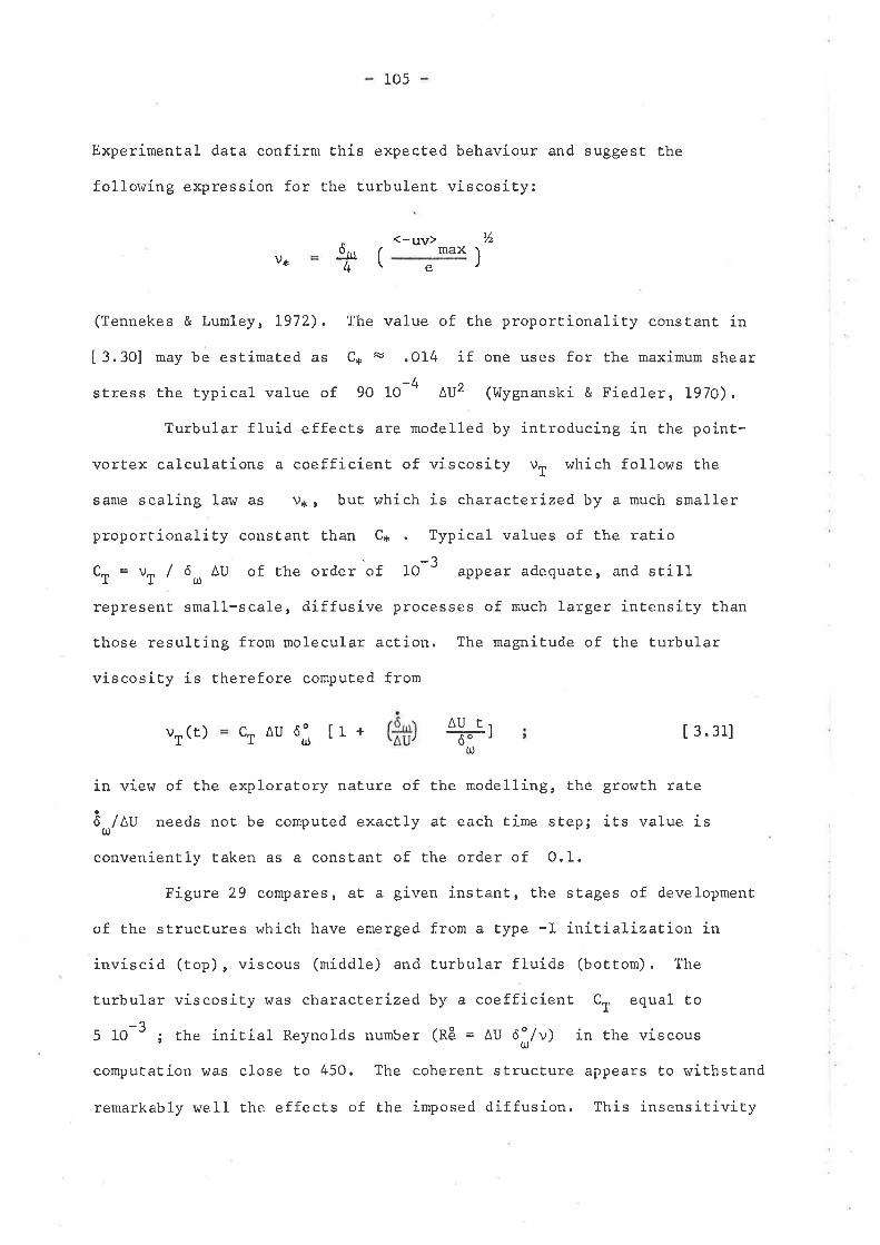
105

Experiment.al data confirm this expected behaviour and suggest Èhe

follorving expression for the turbulent viscosity:

v* fu(4\<-uv> 1A

maxe

v, (t) cr AU ôO(¡)

[1+ AUriõ--

u)

)

(Tennekes & Lumley, L972). The value of Ehe proportionality constant in

[3.3O] may be esÈimated as C* o .014 if one uses for the maximum shear

stress the typical value of 90 1O-4 LIJ2 (tr^lygnanski & Fiedler, 1970).

Turbular fluid effecÈs ar:e modelled by introducing in the point-

vortex calculaÈions a coefficient of viscosity vT which follows the

same scaling law as v* r but v¡hich is characterized by a much smaller

proporEionality constant Ehan C* . Typical values of the ratio

CT = uT / ôur AU of the order of 1O-3 appear adequate, and still

represent smal1-scale, diffusive processes of much larger intensity than

those resulting from molecular acEion. The magniÈude of the turbular

viscosity is therefore compuEed from

l [ 3.3U

in view of the exploratory naÈure of the modelling, Èhe growEh rat.e

8-/¡U needs not be computed exactly at each Èime step; its value is{¡)'

conveniently taken as a constant of the order of 0.1.

Figure 29 compares, at a given instant., the stages of development

of the structures which have emerged from a type -I initialization in

inviscid (top), viscous (midctle) and turbular fluids (bottom). The

Eurbular viscosity was characterized by a coefficient Cf equal Eo

_25 lO-' ; the initial Reynolds number (nå = nU ôi/v) in the viscous

computatiorr \¡/as close Eo 450. The coherent structure appears Èo withstand

remarkably weIl the effects of the imposed diffusion. This insensitivity

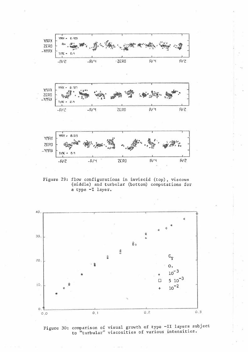
*' .'çrÉ,* ..S"t'.fu" ",n,un# ñï'#y' ;ffi: +$'lß+(. ø.ç13

llllE. ?.1

YNRX

ZERt]_YNRX

J)/e -F/1 ZERO ll/ 1 Ale

YNRX

ZERO

-YNßX

40

30

20

lc

-R/¿ -FlI ZERt] ß/r u/?

TNf]X

ZERt]

-YNRX

-f1/? -F/1 ZERO lll r tì/?

Figure 29: flow configuraÈions in inviscid (top), viscous(middle) and turbular (bottom) computations fora type -I layer.

o.o o.l o.2 o.3

k#"""S"S 'fu,fo" 66'# L#'i#q' ,gf""'lftry - ø.38 1

ïlflE. ?,\

ryfu" "4in,Fs..'m ,#.',H" 'ú'Å#,"r,

TtfiRx. 8.5t5

Ìlf€ - ?"t

r+

*Þ

-3

*)È

o.*

f"*

* cr

*

t

to

*

-3*

u+

o.

10

5

1_O

10-2

o

Figure 30: comparison of visual- growth of type -II layers subjecL" to itturbular" viscosiÈies of various intensities.

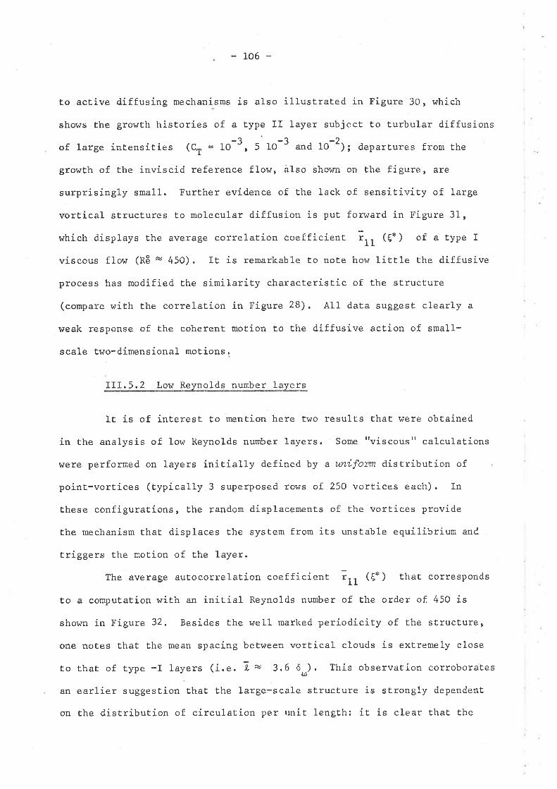
106 -

to active diffusing mechanisms is also illustrated in Figure 30, which

shows the growËh histories of a type II layer subject to turbular diffusions

of large inËensities (CT = 1o-3, 5 1o-3 ana to-2¡; deparÈures from the

gror^/th of the inviscid reference f lov¡, also shor'rn on the figure, are

surprisingly small. Further evidence of the lack of sensitivity of large

vortical structures to molecular diffusion is put forward in Figure 31,

which displays the average correlation coefficient Ir, (E* ) of a type I

víscous flow (nð ^, 450). It is remarkable to note how little the diffusive

process has modified the similarity characterisEic of the st,ructure

(compare with the correlation in Figure 28). All data suggest clearly a

weak response of the coherent motion to the díffusive action of small-

scale two-dimensional motions.

III.5.2 Low Reynolds number layers

Ir is of interest to menlion here two results that were obtained

in the analysis of low Reynolds number layers. Some t'viscous" calculations

r+ere performed on layers initially defined by a m.ifonn distribution of

poinÈ-vortices (typically 3 superposed rows of 250 vortices each). In

these configurations, the random displacements of the vortices provide

the mechanism that displaces the sysÈem from its unstable equilibrium and

triggers the motion of the layer.

The average autocorrelation coefficient Ir, (E* ) that corresponds

to a compuËation with an initial Reynolds number of the order of 450 is

shown in Figure 32. Besides the well marked periodicity of the strucËure,

one noÈes thaE the mean spacing between vortical clouds is extremely close

to that of type -I layers (i.e. lx 3.6 ôo). This observation corroboraEes

an earlier suggestion thaL the large-scale strucÈure is strongly dependent

on the distribution of circularion per unit lengËh: it is clear that the

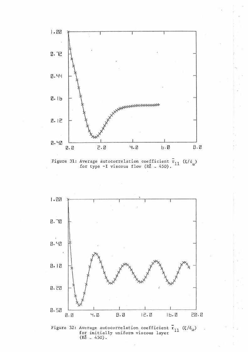
l.Øø

Ø.1¿

ø. tlT

ø. lb

ø. t¿

ø.1Øø.Ø ¿.ø T.ø b.ø

Figure 31: Average àutocorrelation coefficient rfor Eype -I viscous flow (RE - 450).

t "ØØ

ø.)Ø

Ø.lØ

ø, lØ

ø.eØ

Ø.5ØY'-Ø B.ø te- Ø th- Ø eØ. Ø

B.Ø

11 (t/ôor)

Figure 32: Average autocorrelation coefficiert rl1 (t/ôo)for initially uniform viscous layer(RE _ 4so).

-107-

isoLropic nature of the ttvíscoust' random walk tends to generat.e an

effective initíalization ár,.1ogo,-r, to a type -I layer.

Large values of the viscosily may be simply achieved by sufficientty

large amplitudes of the Gaussian displacemenEs. The Èypical evolution of

a highly viscous layer (Rê .- 1) is depicted in Figure 33. It is known

(see for example Batchelor, L962, S 4.3) Ëhat Èhe vortieity t,hickness of

the layer gror,Js linearly with the squaz'e-Toot of. time as a result of

viscous diffusion. The growth history of Èhe layer represented here

indicaÈes clearly thaE the underlying growth mechanism is essentially a

gradienE-diffusion process. This is confirmed by the flow visualizations

(not shown)where no Èendency t.owards clumping into vortical clouds can be

discerned. EfforEs Èowards Ehe precise determination of a critical Reynolds

number for transition are presently undertaken and will be reported

separete Iy .

III.6 SUM},fARY

Broadly speaking, Chapter III presents a study of the motions which

arise when an infinite perturbed vortex sheeL deforms and evolves in iÈs

or¡n induced velociÈy fieId. The vortex sheet is represented by Èhick

periodic vorticity layers; attentí.on is focused on the general properties

of the large-scale structures which are found to ernerge from the vorticity

dísEribuÈions. The relevance of these questions of vortex kinematics to

the turbulenE mixing layer is investigaÈed, on the basis of a temporal

problem which relaÈes to the spatially developing flows through a Galilean

transformaÈion of coordinates

Two specific Eypes of vorticity distributions are considered.

Type I distributions are characÈerízed by a unl,form distributi-on of

circulation per unit length; these of type II have a v,qndom circulat.ion

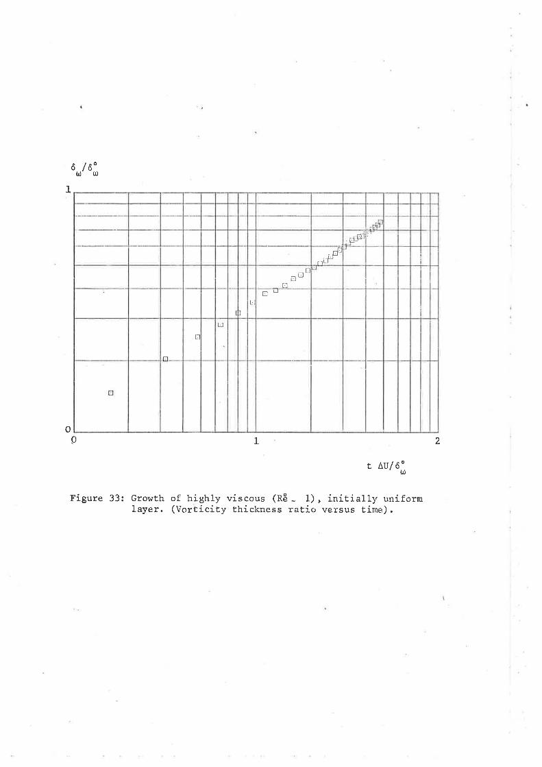
6 /ô'ü) 0J

I

o0 21

t Au/6'

Figure 33: Growth of highly viscous (Rå - 1), initíally uniformlayer. (Vorticity thickness ratio versus time).

.díjÞ

-.F_f

- L:l

LIFl

t

Eo

tr

tr

-108-

per uniE length. The vortex sheet is given a finite thickness by randomizing

the coordinates of the poínt-vortices in the direction normal to the sheet.

Use of the CTC method permits the tìacking of a fairly large number of

vorEices (typically 750) aË reasonable computing costs. Most computations

are carried out in condiËions where the fluid is very nearly inviscid.

Several calculations are also performed to investigate the diffusive acLion

of molecular viscosity and the effects of a small-scale moËion on Lhe

larger flow structures; in these sËudies, diffusion is modelled by adding

a Gaussian random component to the hydrodynamical moEion of the vortices.

Inviscid calculations show in all cases the spontaneous emergence

of arrays of vortical clouds that interact and amalgamate into larger,

clearly identifiable structures. These interactions constitute the

fundamenÈal growth mechanism of the layers. The correlaËion analysis of

the fluctuating velocity fields reveals Ëhe coherent character of the

arrays of structures. All feaÈures of the computed flows appear strongly

reminiscenÈ of those observed in the large sÈructure of the turbulent

mixing layer.

Viscous computaEions at moderate initial Reynolds numbers (-SOO¡

indicate that Ehe structure is remarkably insensiÈive to molecular and

t'turbular" diffusions. At very small Reynolds numbers (-10), viscous

acEion t'killstt the sEructure and the layer gro!üs by a process of gradient

díffusion.

CiIAPTER IV : THE POINT-VORTEX APPROXIMATION OF NON-CIRCULATIONPRESERVING FLOWS

INTRODUCTION

CR.EATION OF CIRCIJLATION IN A FLUID IN MOTION

TV.2.1 Vector flux across a material- surface

TV.2,2 Acceleration, vorticity and expansion

TV,2.3 RaÈe of change of circulaËion

TV.2.4 Bjerknes theorem

POINT-VORTEX MODELLING OF NON CIRCULATION PRESERVINGMOTIONS

IV.3.1 The -fundamental approach

IV.3.2 CompuËaLion of dro/dt

IV.3.2.1 The classical formulation

IV ,3,2 .2 A t'cloud dis cretizationrr formulation

DENSITY EFFECTS ON THE STRUCTURE OF VORTICITY LAYERS

IV.4.1 The temporal problem for two-density layers

IV.4.2 Eff.ect of density ratio on the structure in asinusoidal vorticity Layer

IV.4.3 Froude number effects on the strucÈure in asinusoidal vorticiEy layer

IV.1

rv.2

IV.3

IV.4

IV.5 SUMI'{ARY

109 -

IV.1 INTRODUCTION

All vorÈicity layers studied in chapter III were characterized by

a single parameÈer, the velociÈy difference AU across the interface

between the two uniforn streams. A more general class of shear layers is

that characÈerized by a second parameter, Ap, which represents the

density jump across the vortex sheet. Shear layers beËween fluids v¡ith

different densities are Èhe central subject of the present chapter; their

study is relevant Èo problems as diverse as combustion, jet noise, pollutant

dispersion control and weather prediction.

The lack of understanding of, and the general divergences abouÈ

míxing, entrainment and transport processes in turbulent shear flows (see

Roshko, 1976 & 1979) are a strong motivation for tackling certain aspects

of the mechanics of simple shear flows by developingbasic models; an

atËempt towards the modelling of density aspects on inviscid, non-uniform

shear layers, based on a poinÈ-vortex, CTC calculation, is presented in

the following pages. Although applied Eo a specific case, the scope of

the modelling method proposed hereafter extends effecEively to the broader

class of I'non circulation-preserving" motions. These flows possess the

distinguishing property Ehat Ehe total rate of change of the circulation

around a material curve is not necessarily zero; Ehis is in contrasÈ with

all flows considered so far, for which df/dt did vanish identically.

The general applicability of the present model will be implicit in many of

the arguments to be developed.

Section IV.2 examines the origin and the nature of the mechanisms

capable of modífying Èhe distributíon of vorticíty in a fluid in motion;

the source (sink) of circulation is identified in Bjerknes Eheorem as the

ínEeraction between t,he pressure gradient and Ehe density gradient.

110 -

The modelling of vortici.ty regions by a point-\'ortex approximation

in the presence of density inhomogeneiÈies is considered in Section IV.3,

for the case of incornpressibLe fluids. ft is argued that use of a suitable

discretized form of Bjerknes theorem, coupled with a representation of the

density field based on "density carriers" (i.e. partícles that transport a

density value), provides, in Ëhe spiric of the cloud discretizaËion approach,

a simple but adequate means of analysis. The model relies on the CTC

algorithm as fundament.al computaÈional tool.

The proposed computation method is then applied to the study of

the effecEs of density raEio (and to a lesser extentrofbuoyancy) upon Ehe

structure developing from a sinusoidal vorticj-ty layer of finite thickness.

The results of various numerical experimenEs, presented in Section IV.4,

suggest that the approach followed here, although of limited accuracy,

provides a fírm basis to comprehend and unveil the fundamental aspects of

the physics of Èhe problem.

IV,2 CRNATION OF CIRCULATION IN A FLUID IN MOTION

Let us examine under which conditions the circulation around a

material curve drawn in the fluid changes as the material loop is convected

by Èhe motion. The analysis is better undersEood íf one bears in mind a

theorem and an identity which belong to the study of the kinematics of

conEinuous media, and r¿hich are recalled below.

IV,2.1 Vector flux across a material surface

Consider a vector field q defined everywhere in the domain

occupied by the fluid. By definition, the flux of this vector across a

material surface S drawn in the fluid is instantaneously given by the

expression

- 111 -

ds t 4.u

It ís a theorem that the raËe of change of this flux, as the motion evolves

and entrains t.he surface of reference (always constituted of the same

parLicles), is determined by the relaÈion

I 4.zl

or eguivalently by

dS t4.31

oco>=f 3S

-râq0(q) = ll ii* v ' (q * u) + u(v.q) l

-JS

=TS

a

0 (q) dSlq - (g.Y): * go

t

uwhereDq

DT

is the velocity field,

the rate of change of q

t = Y.: the expansion (rate), and

following the motion (see Truesdell, 1954).a

3

IV.2.2 Acceleration. vorticity and expansion

The acceleration field

description of the moËion as

.âta=U=*+

dE

a ís dírectly expressed in a Eulerían

(u. V) u

but can also be written in the form given by Lagrange:

âu

3 = É *l4y ,rt * 3 r y ,

l+.+7

t 4.sl

where u¡ = Y " : represenÈs the vorticity.

An expression for the quantity 9 = Y * : may be obÈained by taking

Èhe curl of equaÈion [4.5] ; this yíelds

a

G=Vxa=O+0t¡- (o. V) u t 4.61

.LLz-

an expression valid in any fluid and totally independent of the equations

of motion. Note that the identity t4.61 simplifies to

I 4.71

in Èhe case of a two-dimensional moÈion.

IV,2.3 Rate of change of circulation

The previous theorem provides the starÈing point for classifying

possible fluid flows into t'circulation-preserving" and t'non circulation-

preservingrr motions. Recalling that the flux of vorticiÈy : across a

material surface S is the circulation I, one writes

a

9=Y*3=3*03

0 (tt) =f:'c

dGu)(v=f*S

dS=

S

X dS

(o.V)u+0ol.dS

r, I 4.81

where C is the base-conËour or ttsupportrr of the material surface S.

The rate of change of the circulation is then obÈained from f4.21 as

t 4.el

In view of identity [4.6], this result is also expressed as

(Vxa) dS [ 4.10]

One concludes ÈhaE the rate of change of circulaÈion in a moving fluid

. depends critically on the motion being/not being a motion for which I * 3 = O.

The existence of an acceleration potential characÈerizes círculation-preserving

flow fields. The t'source" of circulation arises from the configuration of

the acceleration field; it is clear that further analysis requires the

T ,i <r>t.

= l[,r, -t-S

¡=JS

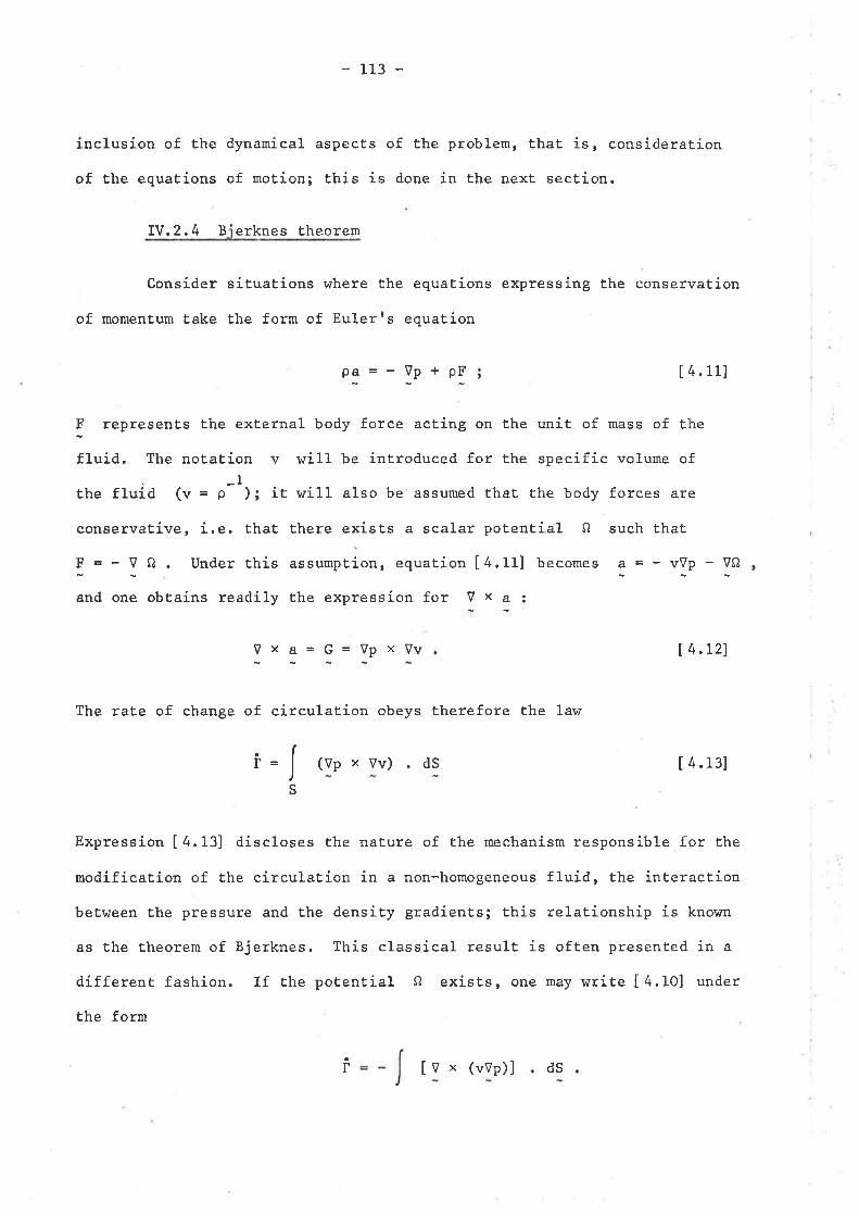
-113-

inclusion of the dynamical aspects of the problem, ÈhaÈ is, consideration

of the equations of motion; this is done in the next section.

IV.2.4 Bierknes Eheorem

Consider situaÈions ¡,rhere the equations expressing the conservation

of momentum take the form of Eulerrs equaLion

p3=-Yp*pl [ 4.lU

I represents the external body force actíng on the unit of mass of the

fluid. The notaEion v wil-1 be introduced for the specific volume of

the fluid 1v = o-I); it hrill also be assumed that the body forces are

conservative, i.e. that there exisÈs a scalar potent,ial 0 such that

þ = - V A . Under this assumpEion, equation [4.11] becomes

and one obtains readily the expression for V x a :

vVp - VQ

Vp xVv I4.r2l

(vp x vv) dS t 4.131

Expression [4.13] discloses the nature of the mechanism responsible for the

nodificatíon of the circulaËion in a non-homogeneous fluíd, the interaction

between the pressure and the density gradients; thís relationship is known

as the Èheorem of Bjerknes. This classical result ís often presented in a

different fashion. If the potential CI exists, one may write [4.10] under

the form

I'i=9=The rate of change of circulaEion obeys therefore the lar.r

i=fs

t I v * (vvp)] dS

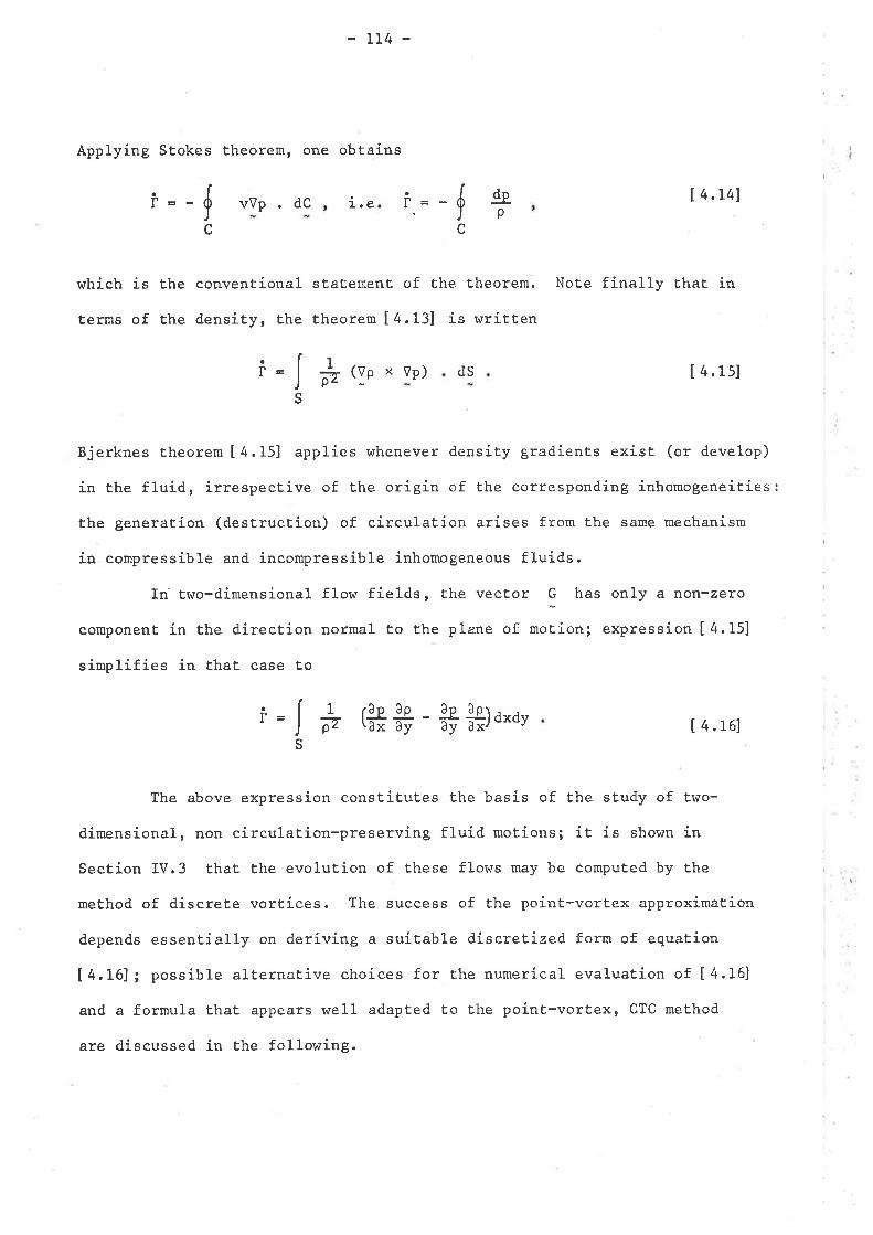
-114-

Applying Stokes theorem, one obtains

vVp . dC 1.e Í 4.L41

which is the conventional staLemenE of the theorem. Note finally that in

Èerms of the density, the theorem [4.13] is written

.tr.= - Ic

.rr=-9c

gP.p

x Vp) dS [ 4.ls]

Bjerknes Lheorem [4.15] applies whenever density gradients exist (or develop)

in Ëhe fluid, irrespectíve of the origin of the corresponding inhomogeneities:

the generation (destruction) of circulation arises from Èhe same mechanism

in compressible and incompressible inhomogeneous fluids.

In two-dimensional flow fields, the vector G has only a non-zero

component in the direction normal to Ehe plane of motion; expression [4.15]

simplifies in that case Ëo

¡=fS

¡t ,Yo

1

æ e# - #*þ*)u"ut t 4.161

The above expression constitutes Ëhe basis of Ëhe sÈudy of two-

dimensional, non circulation-preserving fluid motions; ít is shown in

Section IV.3 Ëhat the evolution of these flows may be computed by the

method of discrete vortices. The success of the point-vortex approximation

depends essenEíally on deríving a suícable dis creEízed form of equation

[ 4.16]; possible alÈernative choices for the numerj.cal evaluation of [ 4,16]

and a formula that appears well adapÈed to Lhe point-vortex, CTC method

are discussed in the following.

¡=JS

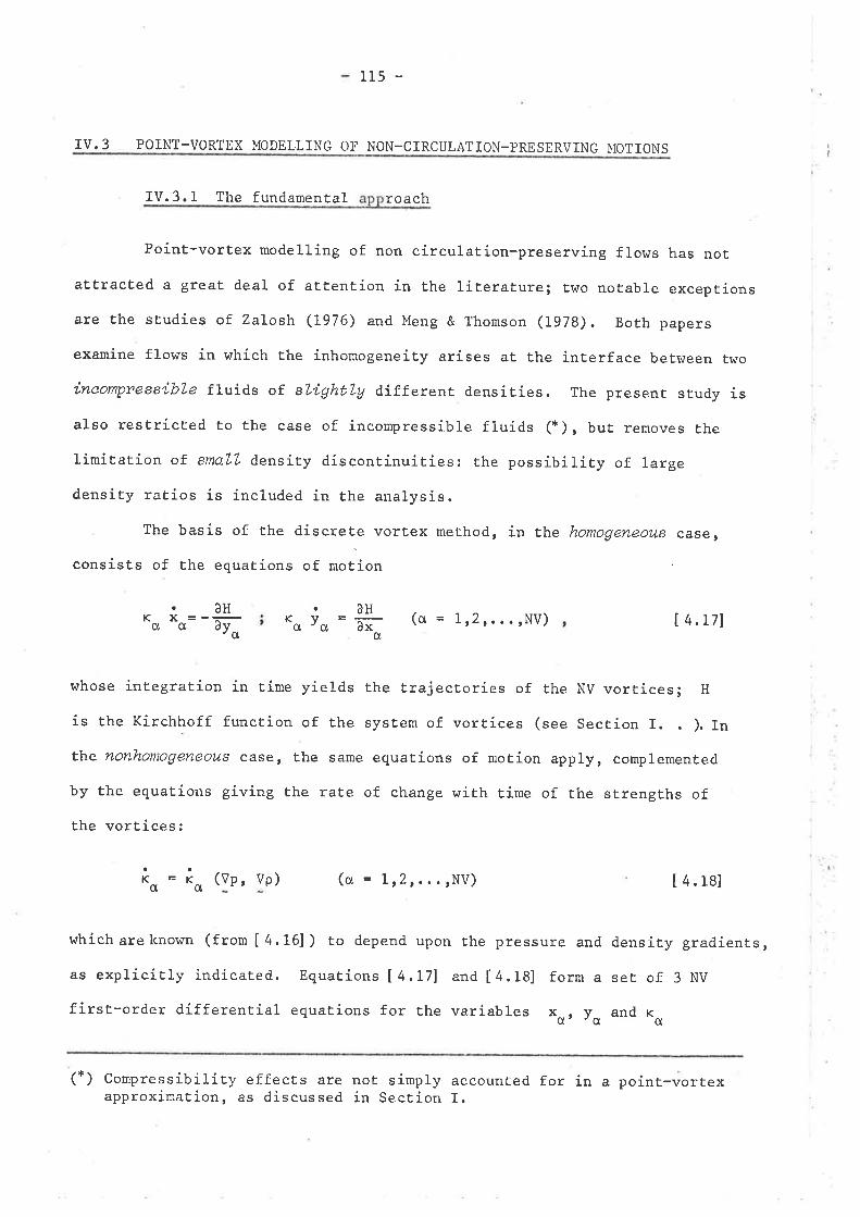
115 -

IV.3 POINT-VORTEX MODELLING OF NON -CIRCULATION-PRE SERVING I'ÍOT IONS

IV.3. I The fun<lamenta1 roach

Point,-vortex modelling of non circulation-preserving flows has not

attracted a great deal of attention in the literature; two notable exceptions

are the studies of Zalosh Q976) and Meng & Thomson (1978). Both papers

examine flows in which the inhomogeneity arises at the interface between two

incontpressíble fluids of. slightly díf.ferent densities. The presenr srudy is

also restricted Èo the case of incompressible fluids (*), but removes the

limitation of smaLZ density discontinuities: the possibility of large

density ratios is included in the analysis.

The basis of the discrete vorÈex method, in the homogeneot¿s case,

consists of the equations of *otiort

K X =-CIgâHr KVc'd

âH (o = 112r.,. rNV) I 4,ttlðxCX

whose integration in time yields the trajectories of the NV vortices; H

is the Kirchhoff function of the system of vortices (see Section I. . ). fn

Ëlae nonhomogeneous case, the same equations of motion app1y, complemented

by the equations giving the rate of change wíth time of the strengths of

t.he vortices:

(vp, vp) (cr - 1,2r...rNV) [ 4.18]

whichareknown (from [4.16]) to depend upon the pressure and density gradients,

as expricitly indicaÈed. Equations [ 4.L7] and [4.18] form a ser of 3 NV

first-order different.ial equations for the variables xq,, yq and ro

(*) Compressibility effects are not simply accounted for in a point-vortexapproximation, as diseussed ín Section I.

K=Kgct

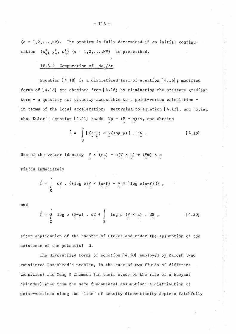
-116-

(cr = 112r,..rNV). The problem is fully determined if an initial configu-

ratíon (

rv. 3. 2 EaLion of dr dr

Equation [4.18] is a discretízed form of equation [4.16] ¡ modified

forms of [4.18] are obtained from [4.16] by eliminating the pressure-gradient

term - a quantity not direcÈly accessible Ëo a point-vortex calculation -

in terms of the loca1 accelerat,ion. Returning to equation [4.13], and noting

that Eulerrs equatíon [4.11] reads Vp = (F - a)/v, one obtains

x v(loe p) I . ds [ 4. le]

Use of the vector identity V x (mc) = m(V x c) + (vm) X

yields inrnediately

dS {(loe p)v x (a-F) - v x [loe p(a-¡)]]

and

1og p (F-a) dc , Í 4,2o1

after application of the theorem of SEokes and under the assumpËion of the

existence of the potential A.

The discretízed forms of equation [4.20] employed by Zalosh (who

considered Rosenheadrs problem, in the case of two fluids of different

densit,íes) and Meng & Thomson (in their study of the rise of a buoyant

cylinder) stem from Ehe same fundamental assumption: a distribution of

point-vortices along Ehe "linerr of density discontinuity depicts faittrfully

oox*r Yot K ;) (o = 1 ,2r, ,. ,NV) is prescribed.

[ (a-F)¡= Is

c

i=Js

dSlogp(Vxa)Í=fc

-TS

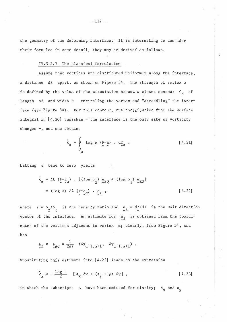
-117-

the geometry of Èhe deforming interface. IË is interesting to consider

their formulae in some detail; they may be derived as follows.

IV.3.2.1 The classical formulation

Assume that vortices are distribuÈed uniformly along the interface,

a disÈance Â.C apart, as shor^rn on Fígure 34. The strength of vortex q,

is defined by the value of the circulation around a closed contour Co of

length At, and width e encircling the vortex and 'jstraddling" the inter-

face (see Figure 34). For this contour, the conEribution from the surface

integral in [4.20] vanishes - the interface is the only site of vorticity

changes -, and one obtains

1og p (F-a) dc I 4 .zLl_ct

.rr =00)c

o

LetEing e tend Ëo zero yields

^.r, (I-3o) { (loe pz) lrQ * (1oe p r) 3ns }

(l-oe s) ^¿

(l-3o) . ?n , I 4.221

where " = pr/pr. i. the density ratio and eU = d!./d0 is the unit directíon

vector of the inEerface. An estimate for ?* is obtained from the coordi-

nates of the vortices adjacent to vortex cÌ,; clearly, from Figure 34, one

has

K0

ôgô=:9, :AC

Substituting this estimate into [ 4,221

# (ô*q-l,o*1, 6yo-1,cr+1)

leads Lo the expression

K + [a*ôx+ (ay=- + g) 6vl 14.231CT

a and av

in which the subscripts CT have been omitLed for clarity; x

\

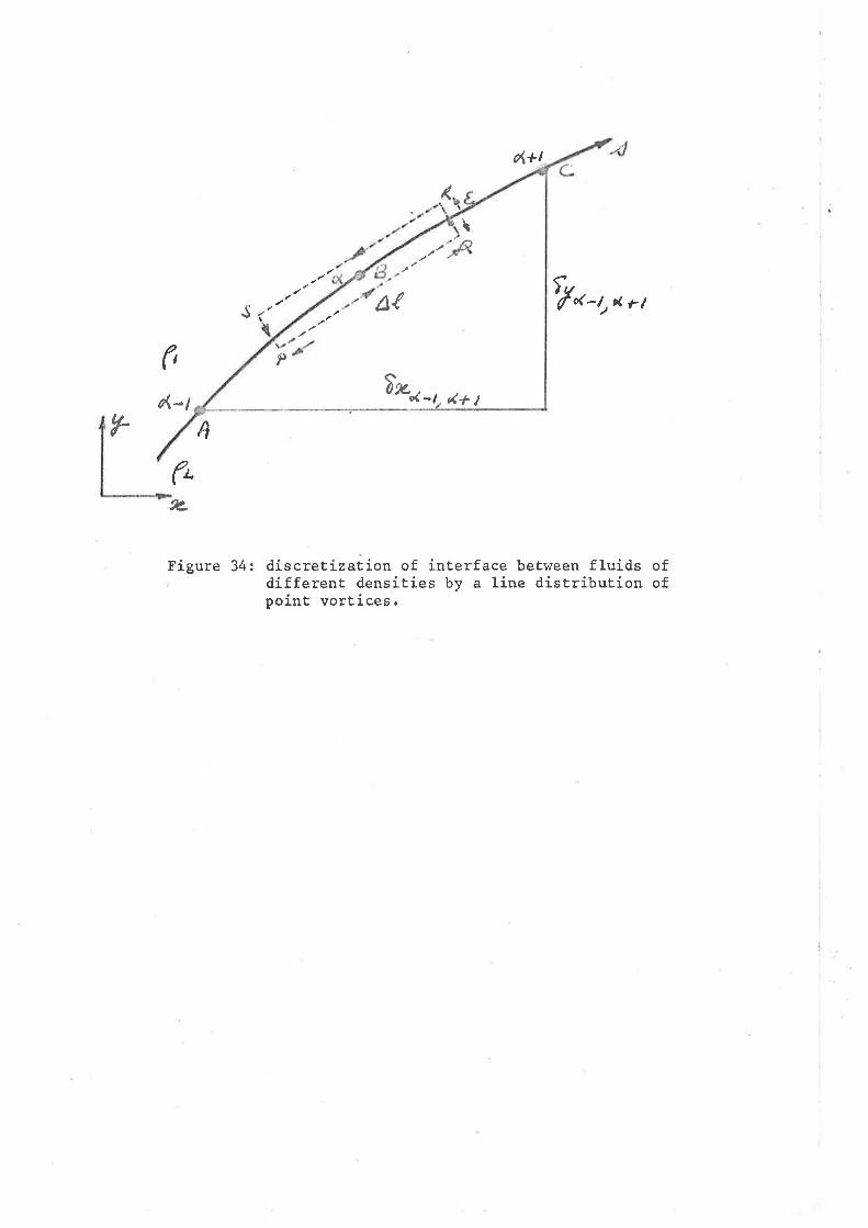
1*u -l 4+t

P

A(

d+l

4

)uf ú-lrc< rts

r('

d,-l/]

Figure 34: discre¿izaÈion of interface beÈween fluids ofdifferent densitíes by a line distribution ofpoint vortices.

(t2

118 -

represent the componenËs of the acceleratíon of vortex cr and g is the

acceleration of gravity. I^tith the additional assumption that the density

ratio s is slightly different frorn unity, Í,4.231 writes (*)

aKvc[ t+Ð [a* ôx + ç + s) 6vl | 4.24a1

this is the approximaÈion adopÈed by Zalosh (1976). In problems v¡here no

shear exisËs initially across the density interface and r+here the motion

from resÈ is induced by buoyancy only, formula I4,241 reduces to

io = (-iä g ôy 1,4.24bj

(Meng & Thomson, 1978)

LV.3.2,2 A "c1oud discretization" formulation

Formulae 14.241 stem from the assumption that Èhe evolution in Ëirne

o1. a singLe row of point-vortices represenËs accurately that of the inter-

face between the fluids. As observed in various studies (refer to the

discussion in Section II. 7 ), Èhe coincidence betwee-n the continuous vortex

sheet and the line whích connects the vortices tends to disappear as the

flow evolves. This geornetrical divergence destroys the validíty of the

approximations Í4,241 at a stage of the computaÈion that seems to depend on

the number of vortices chosen for the discretization. Calculations of the

motion of a sinusoidal vortex sheet in slightly non-uniform situations

(density rat,io close to unity), based on formula [4.24a], were performed;

Èhey were found Ëo break down r¿hen the number of vortices was larger than

40, and sooner as this number r,¡as increased. These results are consisÈent

(* ) Recall that logx=r(#r). åtäl) ' + (x> o)

-119-

\"rith the observation that refining the single-ro\¡r discretization of vortex

sheets tends to trigger the occurence of random movements in the trajectories

of the vortices (refer to Section II.2,Z).

A possible soluEion to these problems, suggesEed and adopted in the

early part of this rsork, is to represent the interface as a thin vorticity

region of fínite thickness, and use sel)eraL xows of vortices in the discre-

Ëization. The increase in definition of the vorticity distribution is then

balanced by the loss in sharpness of the geomet,ry of che interface; use of

equations I4.241 is no longer v¡arranted with this type of discretízation.

The rate of change with time of the sÈrength of vortices used in a cloud

approximaEion was compuËed on Èhe basis of the formula derived in what

fo1lows.

LeË us represenË a vortex sheet by distributing (in a uniform or

random fashion) NV vorEices throughout a layer of finite thickness. Be

AS the area of the material element associated r,/iÈh poinÈ-vortex o.o

Reverting to formula [ 4.19] writt,en in terms of vector component,s, one

obtains the time rate of change of the vortex strength as

dxdy Í 4.2s1

Provided the number of vortices is sufficiently large (i.e. ASo is suitably

smal1), one may approximaËe the integral by considering local average values

of the terms of the integrand; this leads to the esÈimate

¿* (t) = * [.*o (!"rJ, - (aro+ B) (F*)*, . t4.26]

The values of ASo and of po at time È are simply equal to the values

taken at time È = o: in the incompressible case, one has

IAS

KoI 3x. aP\p ðy

ct

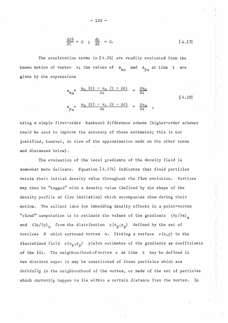
o;

-L20-

dpdr

dASdr

4 x cl

o I 4,271

The acceleration terms in [4.261 are readily evaluated from the

known motion of vortex d; the values of âxc and ayo at Èime t are

given by the expressions

uô¿ (t) u(Y (r - ^r) .s.

AEAE

Í 4.281

Ah.AÈIo

using a simple first-order backr¡ard difference scheme (higher-order schemes

could be used Ëo improve Èhe accuracy of these estimates; this is not

justified, however, in view of the approxímation made on Ehe other terms

and discussed below).

The evaluation of the local gradients of the density field is

somewhat more delicate. Equation [4.27b1 indicaEes that fluid particles

retain their initial density value Èhroughout the flow evolution. Vortices

may then be "tagged" with a density value (defined by the shape of the

density profíle aÈ flow initiation) which accompanies them during their

motion. The salient idea for imbedding density effects in a point-vortex

t'cloudtt computaÈion is to esÈimate the values of the gradients (Ap/ðx)o

and (Ap/ây)a from Ëhe disÈribution O(xU,lU) defined by the seË of

vorEíces Ê which surround vortex o. Fitting a surface p(xry) to the

discretized field O(x6,VU) yields estimates of the gradients as coefficients

of the fit. The neighbourhoodofvortex cr aÈ time Ë may be defined in

two distinct hrays: it rnay be constituted of those particles which are

ínitiaLly in the neighbourhood of the vortex, or made of the set of parÈicles

which cutz,entLg happen to lie within a certain dístance from Ehe vortex. In

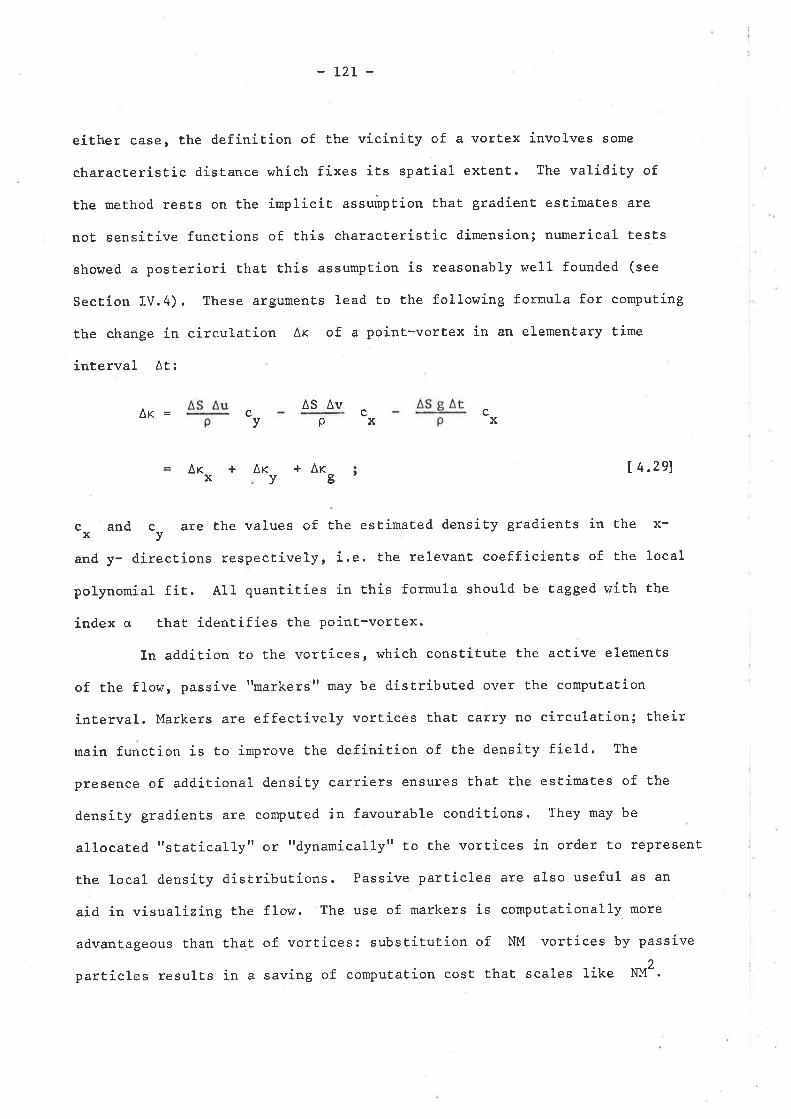
-L2I-

either case, the definition of the vicinity of a vortex involves some

characteristic disEance which fixes its spatial extent. The validity of

the method resÈs on the implicif assuùrption Ehat gradient estimates are

noË sensitive functions of this characteristic dimension; numerical tests

showed a posÈeriori Ëhat this assumpÈion is reasonably well founded (see

Sectíon IV.4) . These arguments lead t,o the following formula for computing

the change in circulaEion Ar of a point-vortex in an elementary time

inÈerval At:

AS AvAr= c

vx

ccv p x x

Ar + Ar +Ar I +.2s1oÞ

c and c are the values of the esEimated density gradients in the x-xyand y- directions respectively, i.". the relevanÈ coefficients of the local

polynomial fit. All quantities in this formula should be tagged with the

index o that identifies the point-vorEex.

In addition to the vortices, which constitute the active elements

of the flow, passivettmarkerstt*"y be distributed over the computatíon

interval. Markers are effectively vorEices thaÈ carry no circulation; their

main function is to improve the definition of the density field. The

presence of additional density carriers ensures Ehat the esËimates of the

density gradients are computed in favourable conditions. They may be

allocatedttstatically" or "dynamicallyt'Èo the vortices in order to rePresent

the local density distributions. Passive particles are also useful as an

aid in vísualizing the flow. The use of markers is computationally more

advantageous than that of vortices: substituEion of Nl"l vortices by passive

particles results in a saving of computatíon cosE that scales like NM2.

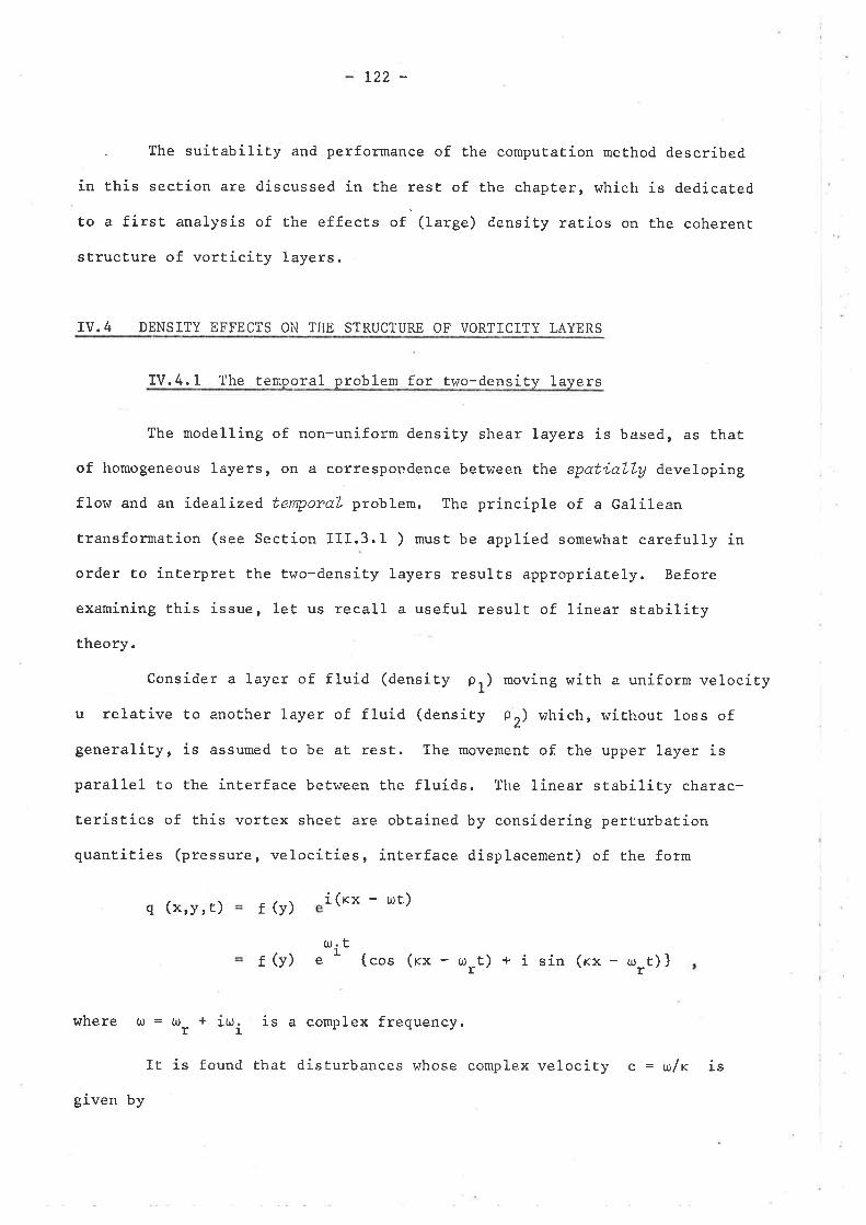
L22 -

. The suitabiliEy and performance of the computation met,hod described

in this section are discussed in the rest of the chapter, which is dedicated

to a first analysis of the effects of (large) density ratios on the coherent

strucÈure of vorticity layers.

IV.4 DENSITY EFFECTS ON THE STRUCTURE OF VORTICITY LAYERS

IV.4.1 The temporal problem for two-densiÈ y layers

The modelling of non-uniform density shear layers is based, as Èhat

of homogeneous layers, on a correspondence between the spatialLy developing

flow and an idealízed tenporaL probLem. The principle of a Galilean

transformation (see Section III.3.1 ) must be applíed somewhat carefully in

order to interpret the two-density layers results appropriately. Before

examining this issue, let us recall a useful result of linear stability

theory.

Consider a layer of fluid (density p1) moving with a uniform velocity

u relative to another layer of fluid (density p2) which, without loss of

generality, is assumed to be at rest. The movemenL of the upper layer is

parallel to Ehe interface between the fluids. The linear stability charac-

Èeristics of this vortex sheeÈ are obtained by considering perturbation

quantities (pressure, velocities, interface displacement) of the form

q (xrY, Ë) r (y) i(rx - ot)

tr (y) e

o1 {cos (rx - u.rrE) + i sin (rx - ,rt) )

where uJ = û) + it¡ is a complex frequency.Ir

given by

It is found that dj.sturbances whose complex velocity c = ufr is

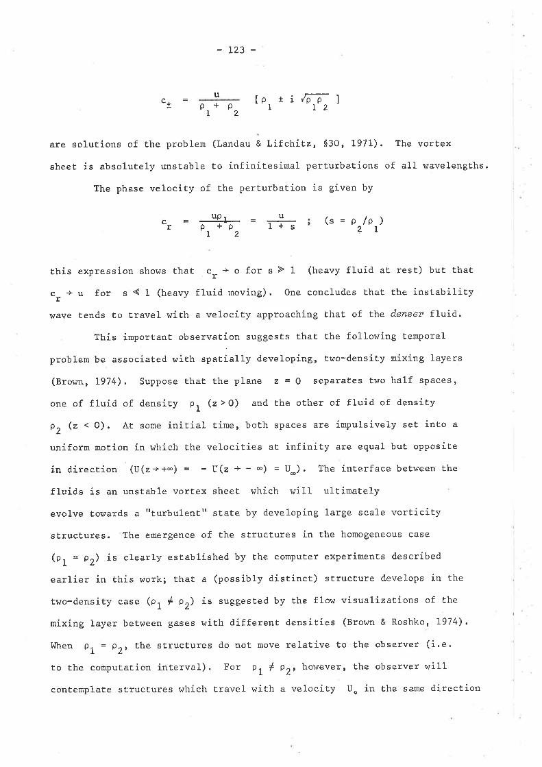
-L23-

c.t +ri4p-l

T2u

p p lp II 2

p2

are solutíons of the problem (Landau & Lifchitz, $30, 1971). The vortex

sheeË is absoluÈely unstable to infinitesimal perÈurbations of all wavelengths.

The phase velocity of the perturbation is gíven by

(s = p /p2

this expression shows that ", * o for s Þ 1 (heavy fluid at rest) but that

c_ + u f.or s ( I (heavy fluid moving). One concludes Ehat the instabilityrwave tends Eo travel wiEh a velocity approaching that of the- densei" fluíd.

This important observaÈion suggests that the following Èemporal

problem be associated with sparìally developing, two-density mixing layers

(Brown, L974). Suppose that the plane z = O seParates two half sPaces'

one of fluid of density pl Q>O) and the other of fluid of density

pZ (z < O). At some initial time, boEh spaces are impulsively set into a

uniform moÈion in which the velocities at infiniEy are equal but opposiEe

in direction (U(z++-¡ = - U(z + - -) = U-). The interface between Ehe

fluids is an unstable vortex sheeE l¡hich will ultimately

evolve towards a ttturbulenttr staÈe by developing large scale vorticity

sÈructures. The emergence of the strucËures in the homogeneous case

(0, = Or) is clearly established by the computer experiments described

earlíer in this work; that a (possibly distinct) structure develops in the

two-density case (0, # O) is suggested by the flow visualizaEions of Ehe

mixing layer between gases r+ith different densities (Brown & Roshko, 1-974),

lrlhen gI = g2, the sÈructures do noÈ move relatíve to the observer (i.e.

to Ehe coÍrputation inEerval). For O, # O, however, the observer rn¡ill

contemplate structures whích t,ravel with a velocity Uo in Èhe same direction

pt

ct rTãuU9t+ )+ t

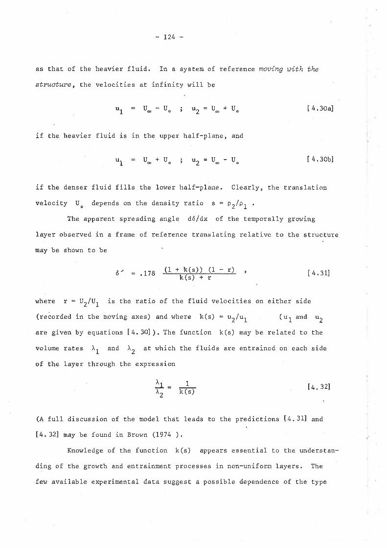
-t24-

as thac of the heavier fluid. In a system of reference moпng uith the

stz,ucture, the velocities aE infínity will be

ttr U6 Uoiuz [ 4.30a]

if the heavier fluíd is in Ehe upper half-plane, and

tl [ 4.30b]

íf the denser fluid fills the lower half-plane. Clearly, the Ëranslation

velocity Uo depends on the density raÈio s = p2/gL .

The apparent spreading angle dô/dx of the temporally growing

layer observed in a frame of reference translating rel-ative Eo the structure

may be shown to be

ô' . L78(1 + k(s)) (1 - r)

k(s) + r [ 4 .31]

where r = lJr/ü, is the rat,io of the fluid velocities on either side

(reäorded in the moving axes) and where k(s) = ur/u1 (u, and u2

are gíven by equations [4.30]). The functíon k(s) may be related to the

volume rates Àt and \Z at r.rhich Èhe fluids are entrained on each side

of the layer through the expression

1 ltr, gzl

(A full discussion of the model tha! leads to Ehe predictions [¿.gf] and

14.321 may be found in Brown (L974 ).

Knowledge of the function k(s) appears essential to the understan-

ding of the growth and entrainment processes in non-uniform layers. The

few avaílable experímental data suggesE a possible dependence of the Èype

U+Uæ

u^=U -U¿@o

U o+Uæ

k(s)\\z

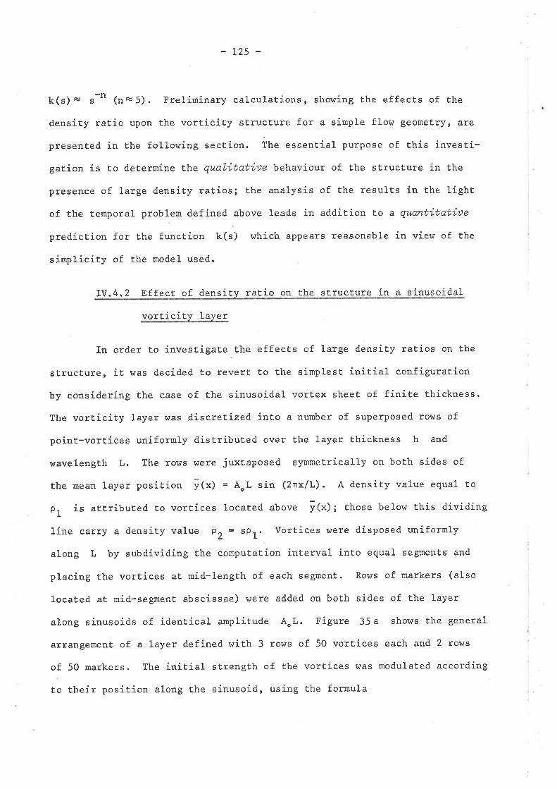
-L25-

k(s)- s-n (n-5). Preliminary calculations, showing the effects of the

clensíty ratio upon Èhe vorticíty structure for a simple flow geometry, are

presented ín the following secËion. The essential purpose of this ínvesti-

gation is to determine tlne quaLitatiue behaviour of the strucËure in the

presence of large density ratios; the analysis of the results in the light

of the temporal problem defined above leads in addition Lo a quantitatiue

prediction for Èhe functíon k(s) which appears reasonable in view of the

simplicity of the model used.

IV.4.2 Effect of density ratio on the structure in a sinusoidal

vorticitv layer

In order Èo investigate the effecÈs of large density ratios on Ëhe

structure, it was decided to revert to Ëhe símplesÈ initial configuration

by considering Èhe case of the sinusoidal vort,ex sheet of finite thickness.

The vorticity layer was discretized into a number of superposed rows of

point-vorËices uniformly distributed over the layer thickness h and

wavelength L. The rows were juxEaposed symmeËrically on boÈh sides of

the mean layer position yt"> = AoL sin (2t¡x/f). A density value equal to

p1 is attributed to vortices located above i("); those below this dividing

line carry a density value P2 = sPl. Vortice-s were disposed uniformly

along L by subdividíng the computation inÈerval into equal segments and

placing the vortices at mid-length of each segment. Rows of markers (also

located at mid-segment abscissae) were added on both sides of the layer

along sinusoids of identical amplitude AoL. Figure 35a shows the general

arrangemenE of a layer defined with 3 rows of 5O vortices each and 2 rows

of 50 markers. The initial strength of the vortices was ¡nodulated according

Èo their position along Ehe sinusoid, using the formula

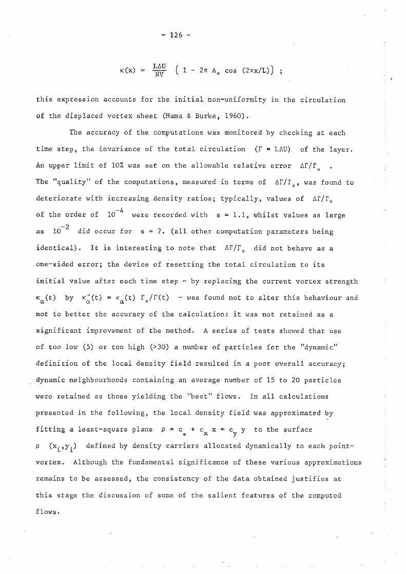
-L26-

r (x)

this expression accounts for the initial non-uniforruity in the circulation

of the displaced vortex sheet (Hama & Burke, 1960).

The accuracy of the computations was monítored by checkíng aÈ each

time sËep, the invariance of the total círculat,ion (I = LAU) of the layer.

An upper limit of LO7. was seÈ on the allowable relative error Af/f.

Thetrquality" of the computations, measured in terms of Af/f., $¡as found t,o

deteríorate \,rith increasing density ratios; typically, values of Af/f.

of the order of 1O-4 \¡rere recordecl with s = 1.1, whilst, values as large

as LO-2 did occur for s = 7. (a11 other computaÈion parameters beíng

identical). It is interesËing Èo note thaÈ ^f/I.

did not behave as a

one-sided error; the device of resetEing the ËoÈal circulation to it,s

initial value afËer each time step - by replacing Ëhe current vorEex strengEh

Ks(t) by ro(t) = ro(t) r./I(È) - rÀras found not Eo alter this behaviour and

not to better the accuracy of the calculation: it was noE retained as a

significant improvement of the meËhod. A series of tests showed that use

of too lorrr (5) or too high (>30) a number of particles for the "dynamic"

definition of the local density field resulted in a poor overall accuracy;

dynamic neighbourhoods conËaining an average number of 15 to 20 parËicles

Ì.üere reLained as those yielding the I'best." flows. In all calculations

presenEed in the following, the local density field r4ras approximated by

fitting a least-squareplane g = co * "*** "rt to the surface

p (xirli) defined by density carriers allocated dynamically to each point-

vortex. Although Èhe fundamental significance of these various approximations

remains to be assessed, the consistency of the data obtained justifies at

this sÈage the discussion of sorne of the salient features of the computed

f lows .

LAUNV It-2nAo cos (2rx/Ð)

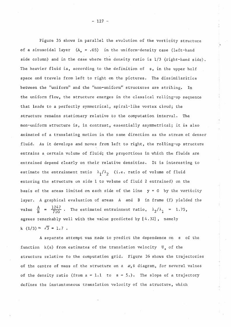
-L27-

Figure 35 shows in parallel the evolutíon of the vorticity structure

of a sinusoidal layer (Ao = .05) ín the uniform-density case (Ieft-hand

side column) and ín the case where thà density ratio is 1/3 (righÈ-hand side).

The heavier fluid is, according to the clefinition of s, in the upper half

space and travels from left to right on Èhe picÈures. The dissimílarities

between the I'uniformil and the "non-uniformil st.ructures are striking. In

the uniform flow, the sËructure emerges in the classical rolling-up sequence

that leads to a perfectly symmetrical, spiral-like vortex cloud; Ëhe

st.ructure remains staÈionary relative to the computation interval-. The

non-uniform structure is, in conËrast, essenËially asymmetrical; it is also

animaEed of a translating motion in Ëhe same direction as the sÈream of denser

fluid. As it develops and moves from left ro ríght, the rolling-up structure

entrains a certain volume of fluid; the proportions in r¡hich the fluids are

entrained depend clearly on their relative densities. It ís interesting to

estimate the entrainment ratio ^L/\Z

(i.e. ratio of volume of fluid

entering the structure on side 1 to volume of fluid 2 entrained) on the

basis of the areas limited on each side of the line y = O by Èhe vorticity

layer. A graphical evaluation of areas A and B in frame (f) yielded the

- A L2/'1value Ë = fr . The estinaEed entrainment ratio, xz/^L = L,75,

agrees remarkably well r^¡ith the value predicted by [4.32], namely

k(L/3)- ß=I.7

A separate attempt was made Èo predict the dependence on s of the

function k(s) from esÈimates of the translation velocity Uo of the

structure relative to the computation grid. Figure 36 shows the trajectories

of the centre of mass of the structure on a ærú díagram, for several values

of the clensity ratio (from s = 1.1 to s = 5.). The slope of a trajectory

defínes the instantaneous translation velocity of the structure, which

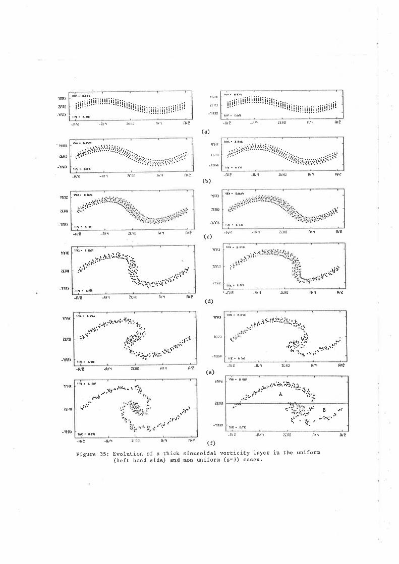
iiii¡iii¡!ii!¡i!¡¡¡i¡¡¡i:¡i¡¡ii¡ii¡i¡iii¡i¡i¡iiiiilrE. l,ø

t.a¡a'ttTtx

ZERO

-YmT

lfl¡ì x

ZIRû

-'YtTlx

-F/¿

-ß/¿

-ßle

.R/E

-ile

-fll\

-RlY

-flll

-ß/rr

-al\

ZERO -nlq

-n/tl

-nl\

-Ã/Ll

ztP0

ZER{l

¿t.R0

¿tn0

IEPO

zÊn0

n/l

ß/'l ßt¿

-tv¿

-lv¿

-IU¿

W.6na

n/¿

¿tn0,tir'

'"fr!la'

tr ¡ä| -ßl¿ .¡l/\

-flt¿ _al,l

IV\ M¿

fv\ n/¿

tut w¿

!r:tl,;t¡f

rvl ile

w1 we

n/r fv¿

ZERO

tnnr

-lnßx

lnFx

ZERO

-tÞnt

lnnr

lÍn0

.lttßt

rnß)(

¿ERO

.INR¡

(a)

(b)

(c)

rnnt

ZERO

.IMIT

Yflft)(

TERO

-tnßx

rnnx

ztR0

-lf'r¡'¡x

ZERO

ZERO n/t

UERO ßiq

2ERIl f1/ I

¡t/¿

lNRT

'j t:t ¡

-'Ttfìx

F/¡(d)

(e)

Ynnx

?Én0

-ltlfll

¡vè

lllrlx

-tnnx

-n/¿

-H/e -R/r zÊflo n/l Ft? (f)

Figure 35: Evolution of a thick sinusoidal vorticity layer in Èhe uníform(left hand side) and non uniform (s=3) cases'

i¡iii¡i!i¡¡iiii!!¡¡¡!!¡iiii¡¡iiiii¡ii¡ii¡iiiiiiiii¡.Ùñ

tm

.r+iiti:ù

tI !G

-.,...niiii¡]i¡i'i'i'.l titztå"".,:.,:.,;¡,,.ni,,r,o.,,.r**rr,f

¡rfr. !.ñ

lN. !.8

llE ¡ a.rl

*t:ï''.-ii!

lrft. a,rú

.,.¡¡'i'if ilii..:lii.lr,._

ì','¡Þ.ri'. À.i.;¡'ìi.'il.r;.

r.,".i¡r. i

lN. a.É

,ff"'i¿i'r

illt . I'tlt

rd. 4.ru

. .r.-".rlrr i' "rl;r'.,.,.,,.ir':i-'

"1i,sii'' ,r#o..11þ.,,:l-.i

ilii.'t

{'îl'r.t

.:fl:i,n

i.:$.i.'i:,'t' , *t -.¡\rì¡-..,., ..-

't.í:

.il'i:tiÍL 'lrr. .',!ri '

,(l

trù I

lr¡f . a,ì¡

.:i:l

-¡drr

, . t',r,}, -. î.F:1.';,.¡.,rm. !.¡m

Ar.Þ.

:{'

, v¡Âä'

Ir[. !.8

lr ¡'"4.

t¿)..' B ¡t

tt

tñ. a.td

t-ilt:,'

t"+i

.O, . itß,; - .. f:,i

ilÈ. l,lt

..'lìr'

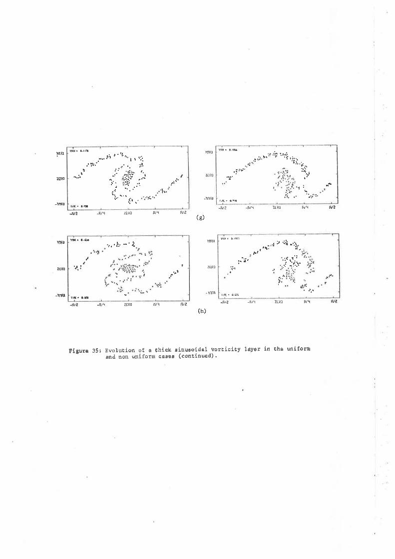
iI

¿/u

eÀ

'(PanuÏluoa) sEFEo roJTun uou PUE

u¡¡o¡Tün eq¡ uT rС{FT Á¡TÐTrro,r'1uploerui¡ lotrr¡¡ e ¡o uoTln1o^it l9€ arntl¡

(q)

h/u0rl¿h/u-2lu-ztnh/t0812hlu-dtv-

dw^

0ülz

xur.lÄ

(t)0d32h/t-¿N' ¿ttth /tl

h/u0ð1¿h/É-¿4'-

xtÀ,\-

fJð32

l&lr-

IUl!Z

IrLtÀ

ÍBrt-

0ù!2

TI¡JA xuüÀ

1

lrt "

t!.....r.

".?.

tPrl ,С

g0.Il

,.1

l.¡'r:';,¿

ii¡. t, .i í.,:tf I r'r

:tr'

¡i

? .- 'T.'','El'l .U

: 'r'.

CË'l , l¡[

l'

a

.?'.'.,ï.i:

;r.' *,i'.i'¿di.s

"

-+: l'

El . al¡

!,l.'¡.

'.r+'. Ët

r" ï1., i;,-" Éìíi ..*'t ":*'il"

.' ;'' .'rr¡""' " | ¡'rt' s 1'1"""

rls'r' h:i

h.¡

t

alt.! ¡

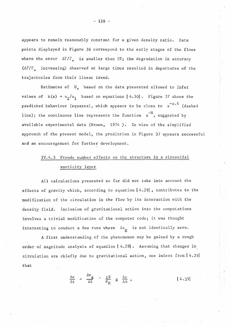
-L28-

appears to remain reasonably constant for a given density ratio. Data

poinEs displayed in Figure 36 correspond to Èhe early stages of Èhe flows

where the error AI/f. is smaller thàn 52; the degradation in accuracy

(Af/fo increasíng) observed at large Èimes resulted in departures of the

trajecEories from their linear trend.

EstimaÈes of Uo based on the daÈa presented allowed to infer

values of k(s) = ur/rt, based on equations [4.30]. Figure 37 shows the

predicted behaviour (squares), which appears Eo be close to ,-o'4 (dashed

line); the continuous líne represents Èhe function "-%,

suggested by

available experimental data (Brown, L974 ), In view of the simplified

approach of the presenË model, the prediction in Figure 37 appears successful

and an encouragement for further development.

IV.4.3 Froude number effects on the structure in a sinusoidal

vortici er

All calculations presented so far did not Èalce into account Ehe

effects of gravity which, according to equation 14.291, conEributes Eo the

modification of the círculation in the flow by its interaction with the

density field. Inclusion of graviÈational actíon into the computations

ínvolves a trivial modification of the computer code; it was thought

inEeresting to conduct a few runs where Ar, is not identically zeto,

A first understanding of the phenomenon may be gained by a rough

order of magnitude analysis of equaEion I 4.291. Assuming that changes in.

circulation are chiefly due to gravitational action, one infers from l4,Zgl

that

ÂrTr

AsPlt

Are

AT4p-Ax

g [ 4.33]

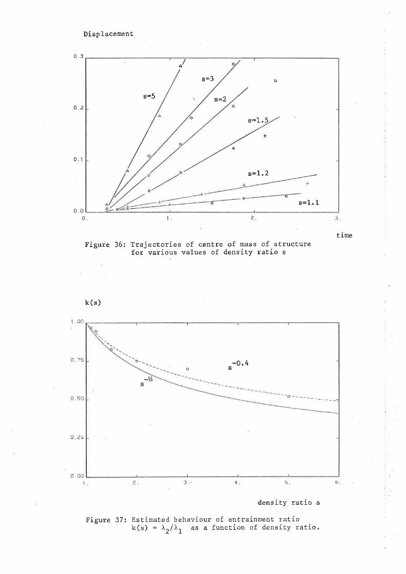
c.3

o.2

Displacement

Figure 36:

0. t

o.oo ¿ 5

Trajectories of cenËre of mass of sLructurefor varíous values of densíty ratio s

time

tco

o.7s

050

o.25

o.ooI

k(s)

z S4'3

density ratio s

EsEimated behaviour of entrainment ratiok(s) = ),r/)'t as a function of density ratío.

s=3

s=5 s=2

s=l.

s=l.2

s=1. 1

o

¿\ o

'*

rfi

E

+

-0.4E s

-û ---.---_--

Figure 37:

6

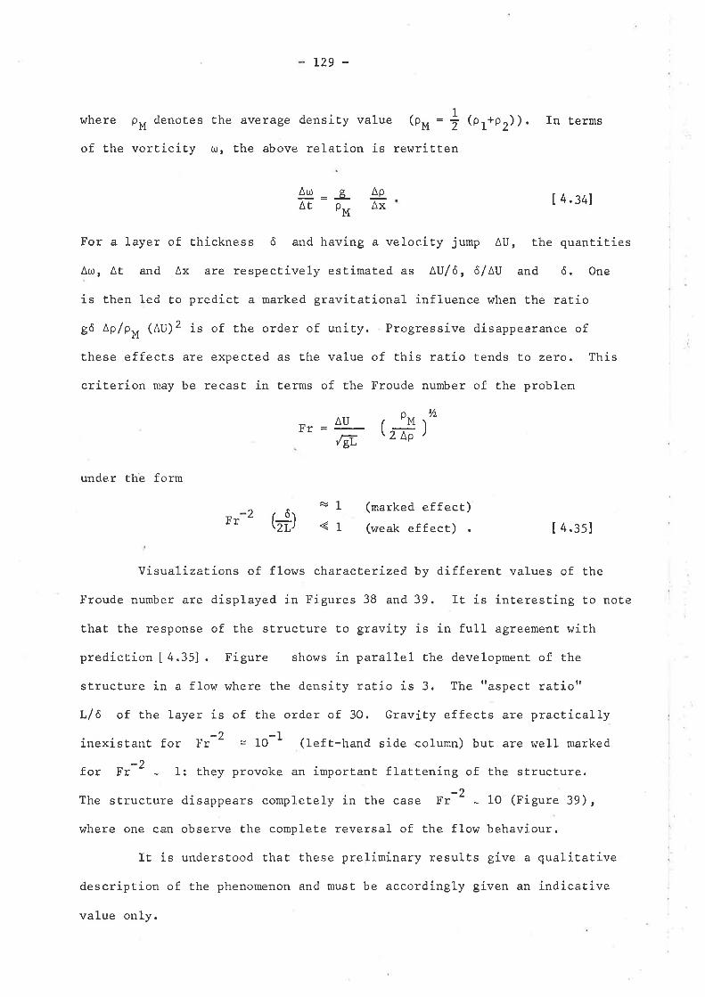
t29 -

$rhere p" denotes the average density value (0" = ! |çr*o)).

of the vorticity o, the above relation is rewritten

Âr¡ _g_pM

ApAx

(marked effect)(weak effect)

In terms

| 4.341

[ 4.3s]

^rFor a layer of thickness ô and having a velocity jump AU, the quantities

Ar¡, ^E

and Ax are respectively estimated as AU/ô, ô/AU and 6. One

is then led Eo predicu a marked gravitational influence when the ratio

gô Ap/pU (AU)2 is of the order of unity. Progressive disappearance of

these effects are expected as the value of this ratio tends to zero. This

criterion may be recast in terms of the Froude number of the problem

AUFrpM

2Ap

tA

( )@

under the form

Fr-L<1

2bi)

VisualizaÈions of flows characËerized by different values of the

Froude number are displayed in Figures 38 and 39. It is interesting to note

Ëhat the response of the structure to gravity is in full agreement with

prediction [ 4.35] . Figure shows in paral1el the development of the

structure in a flow where the densiËy ratio is 3. The "aspect ratioil

L/6 of the layer is of the order of 30. Gravity effects are practically

inexistant for Et-2 = 1O-1 (left-hand side column) but are well marked

for F{2 - l: they provoke an important flattening of Èhe structure.

The sÈructure disappears completely in the case fr-2 - lO (Figure 39),

where one can observe Ëhe complete reversal of the flow behaviour.

IE ís undersËood that these prelirninary results give a qualitative

description of the phenomenon and musÈ be accordingly given an indicative

value only.

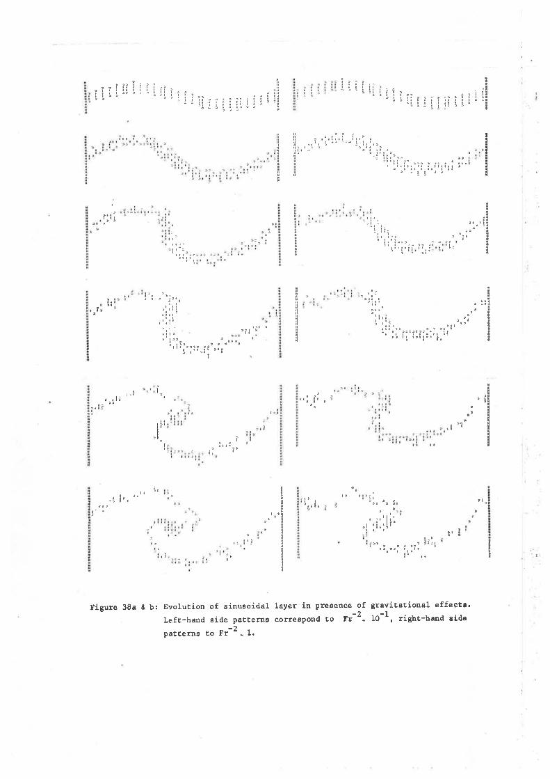
.staæ4|.dE

F

4.-^

ffirñiñ¡rñta.-...rrru4É

ñ

a(r

-,'---:"

ooùr tt(¡{or!

|+{

rg tt

q¡Éqt

âta6tÉ

t tt

o-É.á

è0U

..{

qll{r¡>

Å6t¡{Oö0

Fa

(¡{aO

NI

olþthc¡ooot¡¡-È

!co

'Fl

Àogoq,

s{à¡{qtoror{66É€k.¡o.O

+¡J

ø!

5qlÉ

o.ô¡

.rloqr¡{€krfl

'¡o@

o+

¡É

€oÉ

(¡tr

qt c!

r, -c

l{ato

F-l

u ¡,

o t¡{

r¡>

orqtl¡l

F¡

q

-ôôðqt@(1ol{aào-r{h

n

¡i--^

.=4=

r...=t.:F

¡.tt

rÉ P.

@ É H o (¡, F

0r

r4o< |'1

oH

.F oÉ Þ11

ts.

oo l-tìÞ

0qo

ËH

rÞ P

. H

.rt

Þa o

td

H.

dO. tÞ N'H

¡ts

0tts

<oo ì-'-r

É Þ È o H (n rr H o Þ 0q

0-0

\,

u-0

_ -r

)

0- U -{

)u

--0

U -

-U(r

- r,r-

_ù

u -r

,iJ

__ u -0

u' tr--

r)(/ (/

'U

u- ('- {J-_-u

,_:

rj -U

u-_r

Ju(

l-(,

, _-

--u-

-l)U

--

==

==

:==

==

=ut

)u

0- 0

r)-

tl-t) u-

tl

0---

.Uu --

\,u-

uu-

-(,

- l)

(r -- 0-

-(,

r -u

0- - -u

(r- -u u-

0 -u

UIJ

-.U

o-:u

()-

(l

,_lu

y- -u

-l)tì-

0

o-o -on--0 --0

":-o

ll -O

rl 0t

l-(t

0+

|-()

nr)

|+l)

00 4+-ll

rl it (ì

()+

n

ô ô---

04-

0

ll--

ti

0--0-

-()

(t--

0 -0

0-

r)

r)

==

==

==

o 0 -0

==

==

==

==

-0U u U IJ

-0

0--(

,

0--U

t'--_

0U

--U

tr--

-ùU

--r.

¡u-

-uU

---U

U.-

U

u--l)

(r--

-t¡

U--

l¡(r

---(

,l)-

-{,

U--

trl¡-

--u

0--t

) (l---

u

0 u

0-t)

U -0

(r-+

+ (

)

(i +

+

0 --

(l

0r)

0-r

t,tr

-+

U-+

U

U.

-(t

--0

0 lì

!t 0 0

-130-

IV.5 SIJMMARY

The object of chapter IV is. to discuss the extension of the point-

vortex method to flows in which the material rate of change of the circu-

lation is not identically zero.

The mechanisms which modify the distribution of circulatíon in

non homogeneous fluids are examined for the general case of three-

dimensional motions, and identified as resulting from Èhe interaction

betvreen pressure and densiÈy gradients (Bjerknes Eheorem).

Two-dimensional flows of an inhomogeneous, incompressible fluid

may be studied, in principle, by a generalized form of the point-vortex

approximation. It is suggested that t.he success of Ehe extended meÈhod

depends critically on the use.of a suitable discretization of Bjerknes

theorem. AtÈenÈion is focused on the specific problem of computing Èhe

change with tirne of the distribution of circulaËion at an interface between

fluids v¡ith different densities. The need for a numerícal procedure

adapted to the discretization of the interface as a thick vortex sheet

is demonstrated; a formula which appears to have the required properties

is proposed. The novel approach relies essentially on the use of density

t'carriers" for representing the densiry field in a suitably defined

neighbourhood of a point-vortex.

The generalízed method is applied to study the effects of density

raÈio on the sinusoidal vorticity layer between two fluids of different

molecular weighEs. This simple flow models the behaviour of non-uniform

mixing layers provided the relationship between temporal and spatial

problems is suitably formulated. Results indícate a strong disLortion of

the structure with fundamental modifications of the enÈrainment process.

The model predicts a dependence of Èhe enÈrainment ratio on the density

131 -

ratio that appears to agree \^7ith an analysis of Brown (L974). Qualitative

results are presented which depict the effect of gravity (Froude number

effect) on the structure.

REFERNNCES

.Abe11, C.J. (1977)Pv,oeeedings 6th Australasían HgdrauLics and. FLuíd Mechanics Conferenee,Adelaide, p. 4I5.

Abernatlry, F.H. & Krþnauer, R.E. (1962)Ihe formation of r¡crb.e>< streets;JournaL of FLuíd Mechanies 13, I.

Acton, E. (1976)Ihe npdelling of large eddies in a two-djrrensional shear layer;JourmnL of FLuid MecVøndcs 76, 3.

Acton, E. (f977)A npdetling of large eddies in an axisyi'rrnetric jet; Lecttpe Notes inPhasics 75, Structr:re and }4echanisms of lurbulence, Voh¡re I, SprÍngerveilag.

Batchelor, G.K. (1967)An introduction to ftuid dlmarnics; Canbridge University Press.

Batt, R.G. (f975)So¡re neasurenents on the effect of tripping the tweôirrensional shearlayer; Aína JoutnaL L3.

Bernal, L.P., Breídentl¡al, R.8., Brohrn, G.L., Konrad, J.H. &

Roslrko, A. (1979)On the develo¡xrent of threedjmensj-onal small scales in tr-:rbulent mixinglayers; znd, Syrnp. on TuybuLent Sheat FLous, London.

Birkhoff, G.D. & Fisher', J. (1959)Do r¡crtex sheets irc1l rp ?; Rc. Circ. mat. PaLerrno Ser, 21 8.

Birldroff, G. Q962)Helrrholtz and Taylor j¡rstability;Proe. SWp. in AppLied Mathematics 13, Providence, R.I. : Ams.

Bradshali, P. (f973)Agandograph 169.

Brourand, F.K. & lrleidman, P.D. (1976)Large scal-es j-n ttre developilg mixing 1a1er; JouzmaL of FLuid Mechanics,76, l.

Brourard, F.K. (f-978)BuLLetin A.P.S. 23, P. 1OO7.

Brorarn, G.L. & Roshl<o, A. (1971)The effect of density difference on the turlculent nixing lar¡er;TwbuLent Shear FLous, Agard - CP - 93.

Broum, G.L. & Roshko, A. (f979)On density effects and. large stmcture Ín turJculent rnixing lalners;Jottv,rnL of FLuid Meehanics 64 , 4.

Bro'¡n G.L. (L974)lhe entrainnent and targe stmcture in turbulent mixing layers;F¿fth AustraLasian Confeoenee on HgdrauLics & FLu'id Mechanics,Christdrurdr, Nor Zea1and.

Ckrandraseldrar, S. (fS6f¡Hyd:rcdynamic and Hydrcrnagnetic StabiliQz; Oxford University Press.

Clhand.rsuda, C.,I'trehta, R.D", lrleir, A.D. & Bradstra^r, P. (1978)

Effect of free-stream turbulence on large structu:¡e in ttrrdculent mixinglayers; Journal of FLuíd Mechanics 85' 4.

Chori-n, A.J. & Bernard, P.S. (1972)

Discretization of a r¡crtex sheet, with an exanple of :p11 t{); Univ. CalÍf . 'BerkeLey Eng. Dept, Report E1'4 - 72 - 5.

Orristiansen, J.P. (1973)Nrrnerical sj¡rnrlation of hyd:odlznarnlcs by tÏre netÌ¡cd of ¡nint rrcrbices;JournaL of ComputationaL Physics L3-

Clark, R.4., Verzi-ger, J.H. & Re1molds, W.C. (1977)

Stanford Un-iversity, DePt of Medr. Eng. Report JF - 9.

Clenents, R.R. & Maull, D.J. (1975)llhe representaLion of sheets of r¡crticity by discrete vcrtices;Progress in Aerospaee Sciences 16, 2.

Delæurt, B.A.G. (f977)l,trdelling plane turöul-ent flou¡s with point r¡cÉices : a nurericaloçerirrent; 6th Austz,aLasiatt Hydraulics anå Fluid Meclønics Confez,ence,Adelaide.

Delcourt, B.A.G. & Bior^rn, G.L. (1979)The er¡clution ard energing structure of a r¡ortex sheet in an inviscid andvisæu.s fluid nodelled by a point-rircrtex netlrod; 2nd Syntp. on TurbuLentShear Flous, London.

Dj¡rptalcis, P.E. & Bro'rn, G.L. (L976)fhe mixing layer at. higÈr Relmolds nurlcer : large-structure di¡namicsarrd enLrainnent; JotunaL of FLuid MecVtnnies 78, 3.

Finl<, P.T. & Sohr I{.K. (1974)Calculation of vorto< sheets in urrsteady flcnu and applications in shr-iphydrodynarnics¡ Ienth Syrnpo síun NaDaL Hydrodynønies, Canbridge, Ir4ass.

Fjrk, P.T. & Soh, W.K. (1978)A neç,¡ approach to roll-rp calculations of vortex sheets; Uniuersity ofNeu South WaLes Repont NAV/ARGI 78/L.

F?iedrichs, K.O. (1966)Special Topics in Fluid Dlmamics; Gordon & Breadr.

Hanra, F.R. & Burke, E.R. (1960)Or the rolling-r-p of a rrcrtex sheet; Undu. MæyLand IechnicaL Note BN-22O.

Ho, C.M. & Nosseir, N.S. (1978)The role of c.cLrerent structure in an inpÍnging jet; BuLLetín of theAmerican Physieal Society, I1¡ 23.

Landau, L.D. a Lifshitz, E.M. (f971)Mécan-ique des fluides; Editions lvlir, l{oscrcu"

IÞng, J.C.S. & Thonìson, J.A.L. (1978)Nr¡rerical studies of sone rronlinear hyd:odlznalrLic prcblems by discreterprto< ele¡rent nethods ; JourmaL of FLuid Mechanics 84 , 3.

Milinazzo, F. & Saffrnan, P.G. (1977)Ttre calculation of large Relmolds nr.l.r¡cer two-dinensional flov^l using discreter¡crtices with random walk; JournaL of Computatíonal Physícs 23.

luloore, C.J. (L977)The discrete r¡crte>< a¡proximation of a fínite r¡crbe>< sheet;JounnL of FLuid MecVtanics 63, 2.

Moore, D.W. & Saffrrìan, P.G. (1975)Itre density of organized ¡¡crtices in a turlculent mixÍng layer;JotænaL of ELuid Mechanícs 69, 3.

Kaden, H. (193I)AufwicJ<lung einer r:nstabil-en untstetigkeits fIädreì fng. Az,ch. 2.

Kadcrnbsev, B.B. & Kostomarov, D.P. (1972)lrrlculent layer j¡¡ an ideal two-dinensior¡al fluid; The Physícs of FLuíds15, r.

Kovasznay, L.S. (1977)Coherent structures in turdculent strear flor,,i; Second AustraLasian Confereneeon Heat and Iuja,ss Tt,øtsfer, Sydney.

Kurahara, K. & Tal<ami, H. (f973)Nl¡reri-cal studies of twedi¡rensional r¡crtex notion by a q¡stem of ¡nint-rrcrtices; JourmaL of the PhysícaL Society of Japan 34, I.

Oster, D., ltlygnanski, f ., Dzionfca, B. & Fiedler, H. (1978)Leetwe Notes in Phgsics 75, p. 48, Structure and ¡4edlanisms Ín Tur:fculenæ,Springler-Verlag.

Roserrhead, L. (1931)Fornration of r¡crbices firom a surface of discontinuity; Proceedings RogaLSociety A I34.

Rostrko, A. (1976)Structure of T\¡dcrfent Shear Flcr,¡¿s 3 a nq^r look; Dryden Lecbu:æ, Aiaa74th Aerospaee Seiences Meeting, Ãiaa paper 76-78.

Safftrnn, P.G. (L977)Leeture Notes in Physics 76, pp. 273-306, Springer-Verlag.

Takami, H. (1964)Nurerical operÍnent w"ith d.isc:¡ete r¡crtex a¡rproxirration, with referenceto ttre rolling-rp of a r¡crtex sheet; Dept. Aey,o. and Astton. Stanfoz.d Uní.;.Repont Sudaer 2O2.

Tn-esdell, C. (1954)Ihe kinernatj-cs of vorbicity; Indiana University Præss.

üIatson, G.N. (LOZZ¡Iheory of Bessel Fr:nctions; _Canbridge Univrersity Press.

Itêstwater, F.L. (1935)Ihe nclling-up of a surface of disæntinuity behrind an aerofoil of finitespan;ARCR&M 1962.

Winant, C.D. & Brcp'sand, F.K. (1974)Vortex pairing : the nedranisrn of tudculent mixing-layer grpwth at n'oderateRelmolds m¡rber; JouvvtaL of FLuid Mechanies 63, 2.

üIygrnanslci, I. & Fiedler, H.E. (I97O)The ü¿o-dirrensional rnixing region; Jownal of ELuíd Mechanícs 4I.

lsgrnnski, I., Oster, D., Fiedler, H. & Dziorba, B. (1978)TeL Auiu Uniu. Report SOE 488.

Zaloslr, R.G. (1976)Discretized Sj¡nul-ation of Vortex Sheet Evolution with Buoyaney and Surfacetension Effects¡ Aiaa Jouv,naL f.I, II.

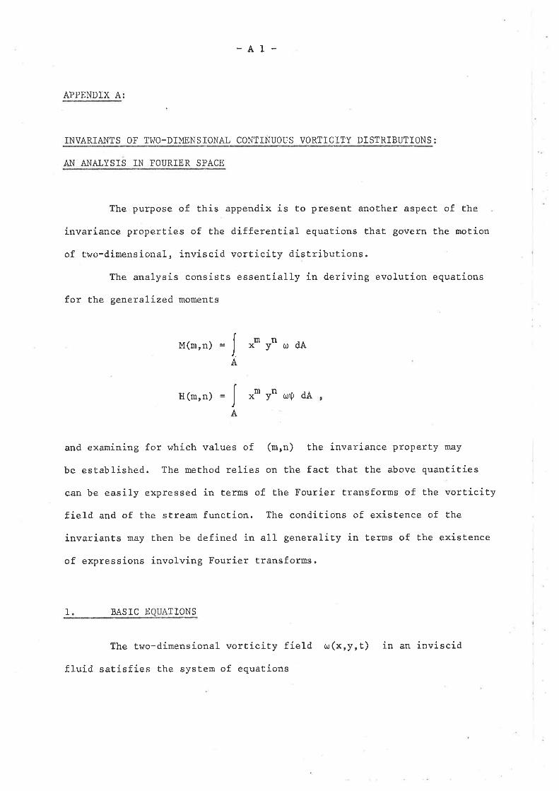
-41-

APPENDIX A:

INVARIANTS OF TWO-DIMENSIONAL CONTINUOUS VORTICITY DISTRIBUTIONS :

AN ANALYSIS IN FOURIER SPACE

The purpose of Ehis appendix is to present another aspecÈ of the

ínvariance properties of the differenÈial equations that govern the motion

of two-dimensional, inviscid vorticity distributions.

The analysis consists essentially in deriving evolution equations

for the generalized moments

M(mrn)

H(mrn) mnx y o!., oA

and examining for which values of (mrn) the invariance property may

be established. The method relies on the fact that the above quantities

can be easily expressed in Eerms of the Fourier transforms of the vortícity

field and of the stream function. The conditions of existence of t,he

invariants may then be defined in all generality in Lerms of the existence

of expressions involving Fourier transforms.

1 BASIC E TIONS

The two-dimensional vorticity fíeld ur(x,y,t) in an inviscid

fluid satisfies the sysÈem of equations

=lxmynu:dAA

=fA

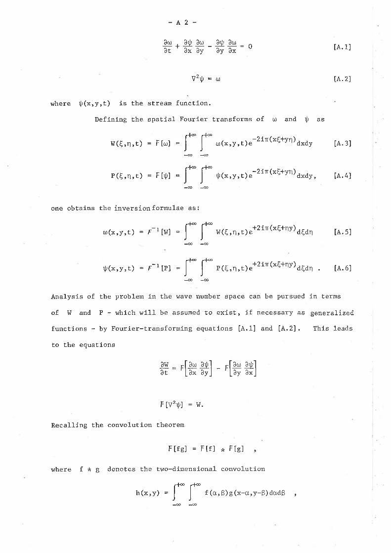
-L2-

!-ü. ât,ây ðx

v'ú=t

where ú(xryrt) ls the stream function.

Definíng the spatíal Fouríer Èransforms of o and !i as

ðr¡ âú ât¡

-+J-_ðt'âxðy

o(xryrt)e -2ín(xE+yn)

lA.ll

lA.2l

dxdy tA.3lI* J*

J* I*

0

I{(E,n,t) = F[rrr] =

trl(x,Y,È) = F-I[I{] =

J* I*P (E,n, t) = F lqrl = rl.r(x,y,t)e

4-oo

-co-æ

-2ir (x[+y¡) dxdy, tA.4l

one obtains the inversion formulae as:

I,{(Ç,¡,t)e+2in(x[+¡y) dEdn [A. s]

-oo-CO

I* J*V(x,Y,t) = F-l [P] = p(8,n,.).*2in(xE+nr)utun tA.6l

Analysis of the problem in the wave number space can be pursued in terms

of I^¡ and P - which will be assumed to exist, if necessary as generalized

functíons - by Fourier-transforming equations [4.1] and [4.2]. This leads

to the equaËions

F tv2r¡.,1 = \4f .

Recalling Ëhe convolution theorem

Flfsl = Flfl x Flel

where f * g denotes the tl^/o-dimensíonal convolution

-æ-æ

ðI^l

ðr F FIlul _ðyJ

laoLa"

ð,¡ !_ü.ðy âx

J* J*-æ-oo

h(x,y) = f (o, ß) g (x-cr,y-ß) dctdß ,

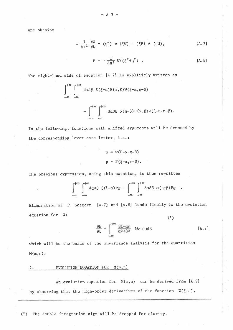
one obtains

-A3-

dodß ß (6-o)P (cr, ß)I,l(E-o,,n-ß)

-##= (nP) * (EI^r) - (gP) * (¡rI),

p = - #r,(82+n2)

The right-hand sÍde of equatÍ-on tA.7] ís explicitly written as

[A.7]

[A.8]

lA. el

f* J*-co-æ

dcrdß o(n-ß)P (cr, ß)\^t(E-o,n-ß) .

In the following, functions with shifted arguments will be denoËed by

the corresponding lower case leËter, í.e.:

w = !ü(E-o,n-ß)

p = P([-c,n-ß).

The previous expression, using this notation, is then rer¿ritten

r -æ

I* J*dodß ß(E-cr)Pw = dcrdß o(n-ß)Pw

-æ-co -æ-æ

Elimínation of P between tA.7l and [4.8] leads fínally to Èhe evolution

equation f or l.I: (* )

âwôr

!üw dodß

2

which will þe the basis of the invariance analysis for the quantities

M(ur,n) .

EVOIUT ION EOUATION FOR M(m.n)

An evoluÈion equation for M(mrn) can be derived from tA.9]

by observing that Èhe hígh-order derivatives of the function I'I(E'n) '

(*) The double integration sign will be dropped for clarity.

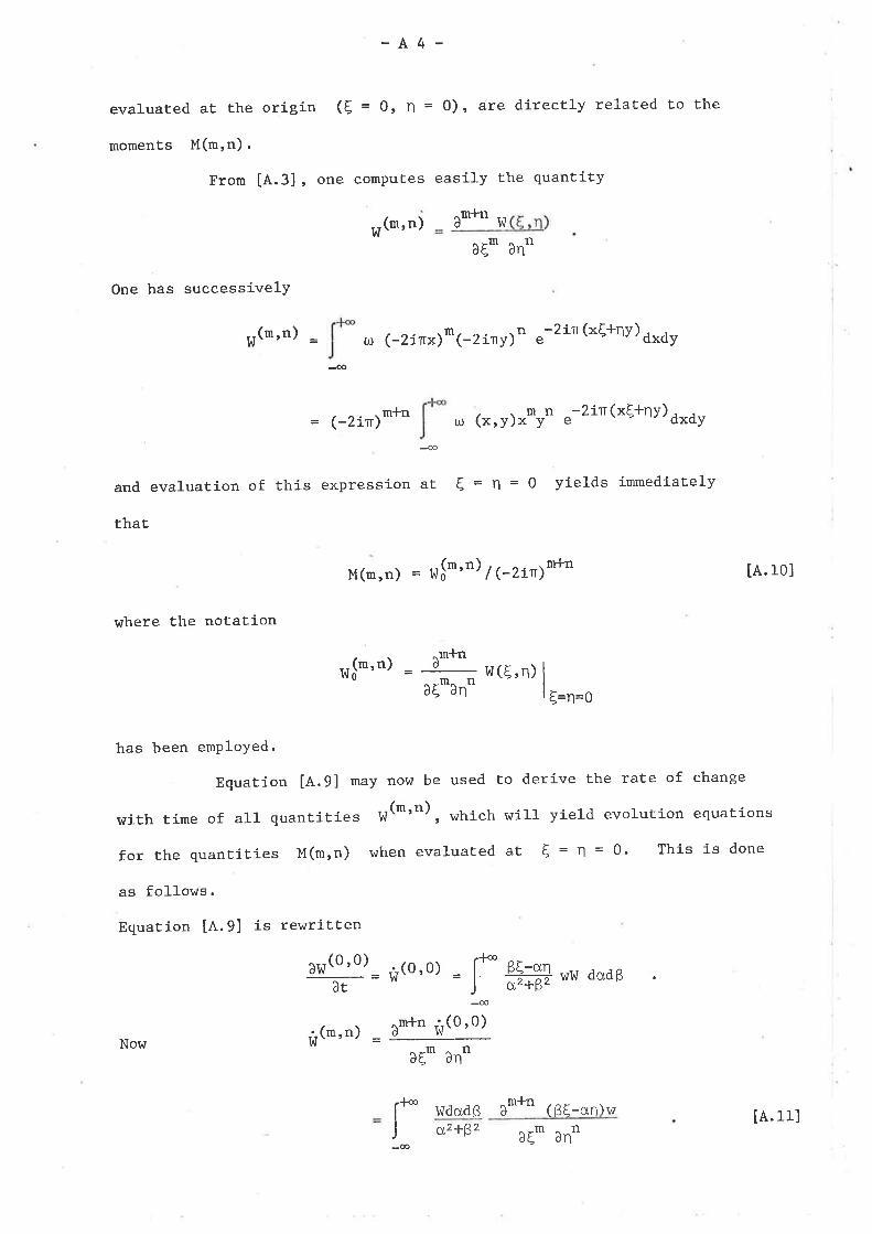
-A4-

evaluated at Ehe origin (E = 0r 1 = 0), are directly related to the

moments l"f(mrn).

From [4.3], one computes easily the quantity

"(mrn)A*+t

ðg* ant

One has successívelY

,,(m,n) -w- ul (-2ínx) m n -2itt(x[+¡y) dxdy(-2iny) e

= (-2ir) m*n mnlrt (x,Y)x Y

-2ín(xÇ+¡y) dxdye

and evaluation of this expression at 6 = rl = 0 yields immedíately

that

M(n,n) = çf*'n)/(-2in)ffi

where the notatíon

I^l

-co

.4

,,(m,n) - ðt+two\"'r"'r =

Ëa,f w{6'n)

|

tA.10l

6=n=o

has been emploYed.

EguaÈíon tA.9] may no\^/ be used to derive the rate of change

with tíme of all quantítíe" "(m'n),

whích will yield evolutíon equatíons

for the quantíties M(mrn) when evaluated at 6 = n = 0. This is done

as follows.

Equation [4.9] is rewritten

!!(o'o)- ,ï(o,o) = |* uç;gl wr,r dodß---ãE-= * J cl-+Ê2 "r'| gwsH

Æ

¡(m,n) - unrrn "(o'o)

ðã* ant

f*l_

m*nI,ldodßa21ß2

(ßË -on)w

Now

o

aEm ônn[A.11]

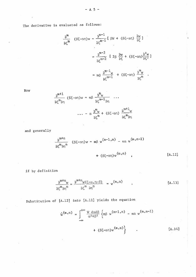
-A5-

The derivative 1s evaluated as f ol-l-o¡'rs:

m$

Now

aE

^m-1(ßE-*n)w = Ë[ ßw + {or-on) ffl

=Ë t2ß#+ (ßE-'n)ffit

^md

ðE -1* <sg-on) +

^I[+1 ^ü- -A"'- (ßE-an)w = *ß #r-aE*an ðE"'^ðn

-m ^m*1oôr+(ßã-on)

âE aE"'ðn

^m-1d \¡7

(ßE-crn)w = rg "(m-1'n) - ,to t(m'n-l)

+ (ßE-o,n)w(m, n)

and generallY

âmln

aElnann

I,I(rn,n)

â*f"w -cx (mrn)

t lA.12l

[A.13]

if by defínition

= !ü¡

ðãt an

Substítution of tA.12l into [A'11] yields the equatíon

ll

þo ,(*-r'") - ,ro r(m'n-l)

-co

l.I+ (ß6-on)w

(mrn) lA.14l

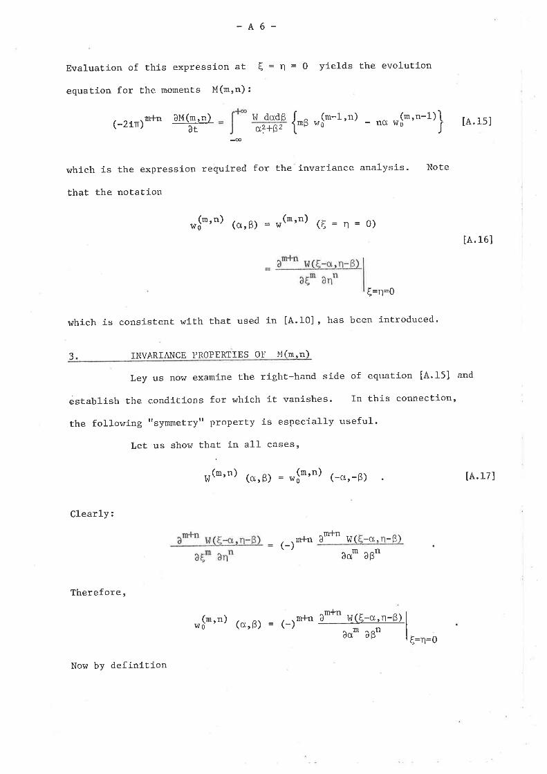
-A6-

Evaluation of this expression at 6 = n = 0 yields the evolution

equation for the moments M(rn,n) :

(-2itr)

whích is the expression required for the invaríance analysis.

that the notation

,o(t,t) (o,ß) -r(m,n) (6=n=o)

rrl-n âM(m,n)ât

I^1 dsdßazt\z {*u 'Í*-t'n) - n0 wsm'n-l)l'

Note

lA.Isl

lA.16l

-æ

3

E=n=o

whích is consistent l^lith thaÈ used in [4.f0], has been introduced'

INVARIAì{ CE PROPERTIES OF lf (rn. n)

Ley us now examíne the right-hand side of equation [4.15] and

esÈablish the conditions for which it vanishes. In Èhis connection,

the following t'symmetrytt Property is especially useful'

Let us show that in all cases'

"(m,n) (a,ß) = ,(*,n) (-s,-ß) tA.17l

Clearly:

urtnm+n A lr( -o. n-ß)= (-)

âo* ôßt

Therefore,

o,$*,t) (o,ß) = f .orrn at+t w(E-cl,n-ß) |'-) *"f I

Now by definition

E=n=o

-A7-

and hence

tü(nrn)

(m,n) (ro r r)0

M(o,o) = trl dxdy

ís invariant.

(b) m=1n=0

One obÈains from [4.15]

}T (-ct,-ß) = \¡r (s, ß)

which is equívalenÈ to [4.17]

The invariance of the lower order moments may noI¡l be proved as follows.

(a) m = n = 0.

Inspection of tA.15l shor¿s that ù(O,O) vaníshes, so

that

lA.18l

lA.lel-æ

(-2in) $ "ct,o) =

J*- u'g (0,0)

I¡7

-æ

Now from [4.16] one knows that

(0,0) (0,0)úI (o,ß) = w (-ct,-ß)

0

so thaÈ

(-2in)

The integrand ís an odd function in (ctrß) and hence its

tnÈegral vanishes identically. Therefore

M(l , o)ðt å#t w(cr,ß)I^r(-c,,-ß)

M(l ,0) =

-æ

is invaríant.

x trl dxdy [A.20]

-A8-

(c) m=0 n=1

Repeating Ëhe argument developed for the case (m = 1,

n = 0) establishes the invariance of the moment

M(0,1) = y trt dxdy.

-6

lA.21l

lA.22l

(d) (m= 2¡ û= 0) + (rn= 0, n= 2)

The evolution equation for the combination I = M(2r0)

+ M(0,2) is obtained from [4.15] as

(J!)"!We,o)+M(0,2)l2 d,t

= [* " rut-ug t:ß ,Í1,0) - o o,$o,r),J az¡gz '

-æ

where, by defíniÈi-on

,Í1'o) = "(1'o)

(-o,-ß) =

(00,1)

AI,I(-o¿,-ß)âa

T^7 = \af(0,1)

The invariance of I is proven íf one establishes the

ídentÍty

Mt=Mz

where

ð Aw (-cl¿, -ß)ôuMr= W dcrdß [1og (o'+ß') ]âß

and

(-*,-ß) =U*g

..4

þ12 = J* " acxao fr tros (a'+ß')l âI^l ( -cr. -ß)

-co

where use has been made of the facÈ that

aß

-A9-

1â tog (o,2+gz )2ò3

The expressions for Ml may be transformed as follows

by carryíng ouÈ the integration o r. to ß

').d, 1â

åF=;*log(crz+$

l"LL = J*u. J* uß+1og(cr2+g2) "#

f_

-co

dcr {lt"r(o'+ß') " #" ]ßr

ßo

J* uu rog(crz+g2, + [âI^I

âcr

dcrdß 1og (a"+g'>

l)w

-æ

tutl = [Mf] f* f*[aw aw-

Læ a"

)

-oo-co

where [M1] rePresents the integrated term.

Identícal manipulations on t1'2 yield the expression

t, = I aø{fr.s(a'+s') "+-J",

J* uo Los(az+gz, * [ðI,{-to aß

= rM2r J: f- u*u log(cr2+e2,[# Eb . " # ]

-ó

Both integrated t,erms vanish provided the vorticity

distributíon vanishes suffíciently rapídly toward

Ínfinity. It is readily seen - wíth the change of

-A10-

variables o, + -0; ß * -ß - that the identíty Ml = M2

Ís verífíed ín this case, which establishes the invariance

of the expressíon

f= (*'+y') trl dxdy fþ,.22)

EVOLUTION EQUATION FOR H(m.n)

Defíne the function 0 (x'y) as the product

0(x,y) = ü(x,y) t¡(x'y) lA.23l

and its Fourier transform F(E'n) by

-@

4

F(E,n) = I* J* 0(x,v) e-i2n (xE+yn)l^.241

lA.2sl

lA.26l

Í^.271

dxdy

-æ-@

with the corresponding inversion formula

2it (x6+yn)0 (x'y) =

It Ís easíly shown that one has

= (_2ír) rrl-n nx v Q (x,y) dxdy

(m, n) m*n

ís easily obtained from [4.7] and

Clearly then

F(E,n) e dEdn

-æ-co

m

(0,0)

so Èhat

The equation giving

[A.S] by notíng that F = I{ * P.

H(mrn) = F 0(-2in)

The invariance of the moments H(mrn) may be ínvestigated by

consideríng the evolution equation for the quanÈitie= r$*'t).

f.*)

âFðr

-A11 -

åË = - 4tr2 p * {(Ew) * (nP.) - (n}r) * (6P)

= 16na p * [(83+En2)p * np - (nt+n6')p ,. (EP)]

afËer repeaËed use of [4.8]

The foregoing expressíon may be rewrítten as

S = ront r(E,n)

where T(E,n) ís gíven bY

T(E'n) = (g2+ß2)P(o, ß) do,dß

f*uudv (ou-ßv)P (u-cr,v-ß)P (6-u,l-v)

-CÐ

f*J

lA.28l

lA.2el

lA.3ol

-oo

In particular,

-- L6tra T (o , o)

ín view of expression [4.29].

=0

This completes the proof that the quanËity

H(0,0) = H = tf trt dxdy

is an invariant of the vorticity distributíon.

Intuitively, one suspecËs that the treatment of vorËices in

Fourier transform space should lead to economics ín Computer Èime

requírements, but this approach has not been pursued further at the

presenË time.

-æ

f*l_

-81-

APPENDIX B:

STREAM FIJNCTION AND INVARIANTS FOR THE DISK OF UNIFORM VORTICITY

The integral,

1

4-, fD

los R;a dt(Q){, (P) ur (Q) [ 8.1]

defining the stream function associated wíth a distribution of vorticíty

o(Q) over a bounded domain 0 can be explicitly evaluated for the

parEicular case of the disk of uniform vorticity, for which one has

rrl(Q)=constant=o0

0 ={(x,y) zx2+t24a2}

The positions of P (fixed)

terms of polar coordinates

One has

(element of domain D) are expressed in

and (r,0) (refer to Figure 8.1) .

and a

(p,0 )

(x(P),Y(P)) = (P cos 0,0 sin q¡

(x(Q),y(Q)) = (r cos 0, r sín 0)

*itq = t2 - ztP eos (e - 0) + P2

dt(q) = r dr d0 ,

and expression IB.1] ís rewritten

a 2r

'J/ (P)

It is easily shown that

o0_

4r rdr d0 log lx2 - 2rp cos (O 0) + p2l tB.2l

d0 log [t2 - 2rp cos (0 -O ) * p2 |

2 Jt uu t.", lr2 - 2rp cos o + p2 l

-82-

so that [¡.2] is rewritÈen

This expression may now be evaluated on

Ír2 - 2rp cos 0 + p2 l. tB.3l

{ t", (^2 - 2AB cos a + 82)

t(P) = ä* lo rdr f uu r.",

te r2nrc=u,0 I I 13drdo

'o 'o

the basis of

2n log Ado={

2n log B

the formula

(A>B)

(B>A)

(ArB > 0), Ëaken from standard integral tables.

The integrat,ion with respect to 0 in tB.3l must be carried out differently

if rÞ p or if r < p. Thís leads Èo distinct forms for the stream

function depending on whether P lies inside or outside the disk. One

finds easily the Èwo forms:

ls.¿l

I B.s]

lB.6l

tB.7I

ú(P) = -

ri(P) = -

G-2

tJ0

4

log P

(p2 - ^2)

(p> a) (P exterior)

log a (p ( a) (P interior)

The ínvariants of the vorticity distribution are easily evaluated

from their definition integrals [1.16], [1.2o], IL.221 and [1,25]. Their

values are:

(a) Total circulation f

f =.(ljo

(b) Coordínates of vorticity centre (X,Y)

X=Y=O

(c) Monent of inertia C (= t2)

f ,rt dr = n,s 2a

1.e G = a2/2 or t = alñ , I B.B]

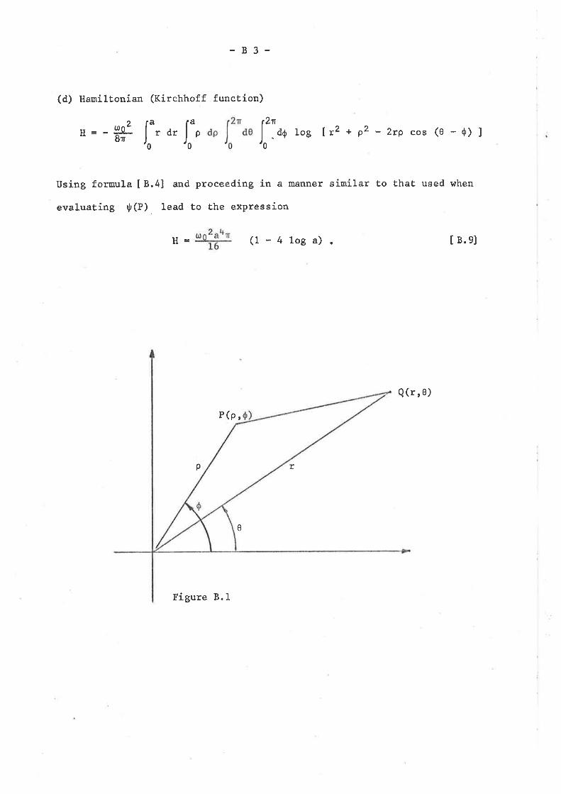
-83-

(d) Hamiltonían (Kirchhoff functíon)

rUsing formula [ 8.4] and proceeding in a manner simíIar to that used when

evaluating û(P) lead to Èhe expression

"=-ä*'f'rZtt

I .uO los It2 * p2 - zrp cos (e - 0) l,0

pdr

!l=

P(p,

p

Figure 8.1

(1-41oga).

r

I B.e]

Q (r, o)

0

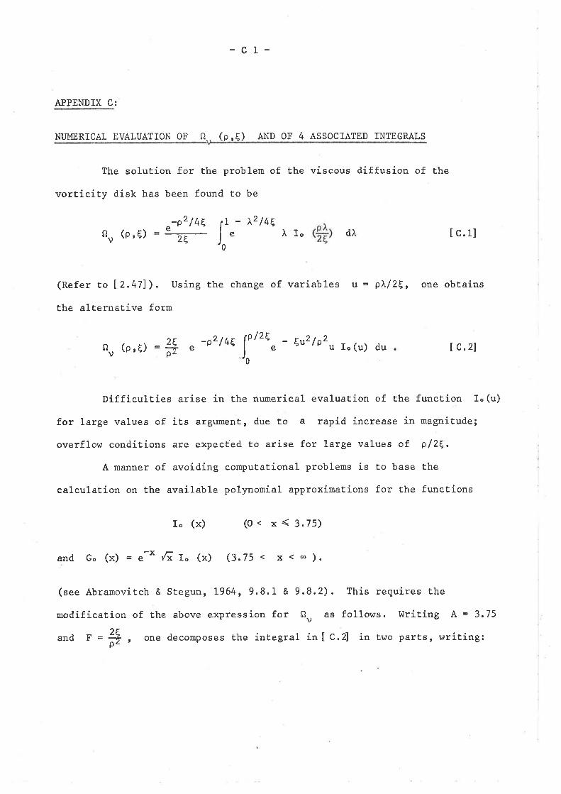
-c1-

APPENDIX C:

NUMERICAL EVALUATION 0F 4.. (p,t ) AND OF 4 ASSOCIATED INTEGRALS

The solution for the problem of the viscous diffusion of Èhe

vorticity disk has been found to be

-p2 / 4E - )\2 /48e À Io dÀ lc.rlou (p,t)

2Ee

(Refer to 12,471). Using the change of variables v = p)'/21¡ onê obtaíns

Ëhe alÈernative form

(p,€) e2 /trE

/2E - Euzlpz u Io (u) du lc.2le

Difficulties arise in the numerícal evaluation of t,he function I" (u)

for large values of its argument, due to a rapíd increase in magnitude;

overflow condiËions are expected to arise for large values of g/2E.

A manner of avoiding compuEational problems is to base the

calculation on the avaíIable polynomial approximations for the funcËions

Io (x) (o < x ( 3.75)

and Go (x) = "-* G. t" (x) (3.75 < x < - ).

(see Abramovitch & Stegun, L964, 9.8.1 & 9,8,2). This requires the

nodif ication of the above expression for Ou as follows. I^Iriting A = 3,75

t,and E = +, one decomposes the integral inI c.Z] in two parts, writing:

l

ov

_2E-æ f-p

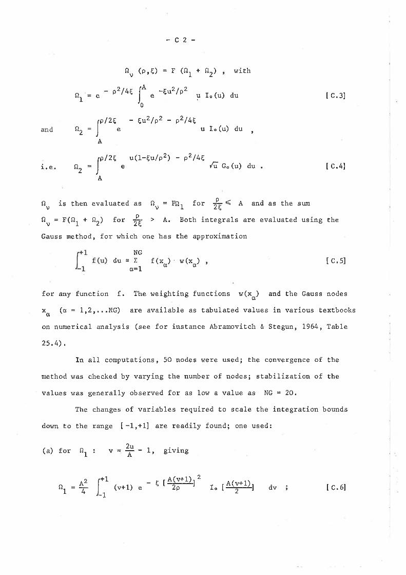
-c2-

0v

(p,E) = F (0, +

/2E

/2E

- Euz /pz - p2 /trEe

u(L-Eu/pz) - pz /trEe

f "-t"r,r, u ro(u) du

withoz)

p2 /ttlot

and a2

=ô I c.3]

Ic.s]

rA

rA

u Io (u) du ,

1.e ç¿

O is then evaluated as CI =vvQu=Flor+ar) for + ) A.

Gauss method , f.or which one has

Æ c" (u) du t c.¿I

Ff¿. for f= < A and as the sumL¿I

BoLh integrals are evaluaÈed using the

the approximation

f (xo) ' w(x*)

2

NG

du=Xcl= 1

for any function f. The weightíng functions w(xo) and the Gauss nodes

*o (cl = 1r2r...NG) are available as ËabulaËed values in various textbooks

on numerical analysís (see for instance Abramovitch & Stegun, 1964, Table

25,4) ,

In all computations, 5O nodes were used; Ehe convergence of the

method was checked by varying Èhe number of nodes¡ stabilization of Èhe

values r^ras generally observed for as 1ow a value as NG = 20.

The changes of variables required to scale Ehe integration bounds

down Èo t,he range [ -tr+t] are readily found; one used:

(a) for ot : v = å9 - t, giving

,,, = f li (v+1) e - E r+Pr' ror$ur dv lc.6l

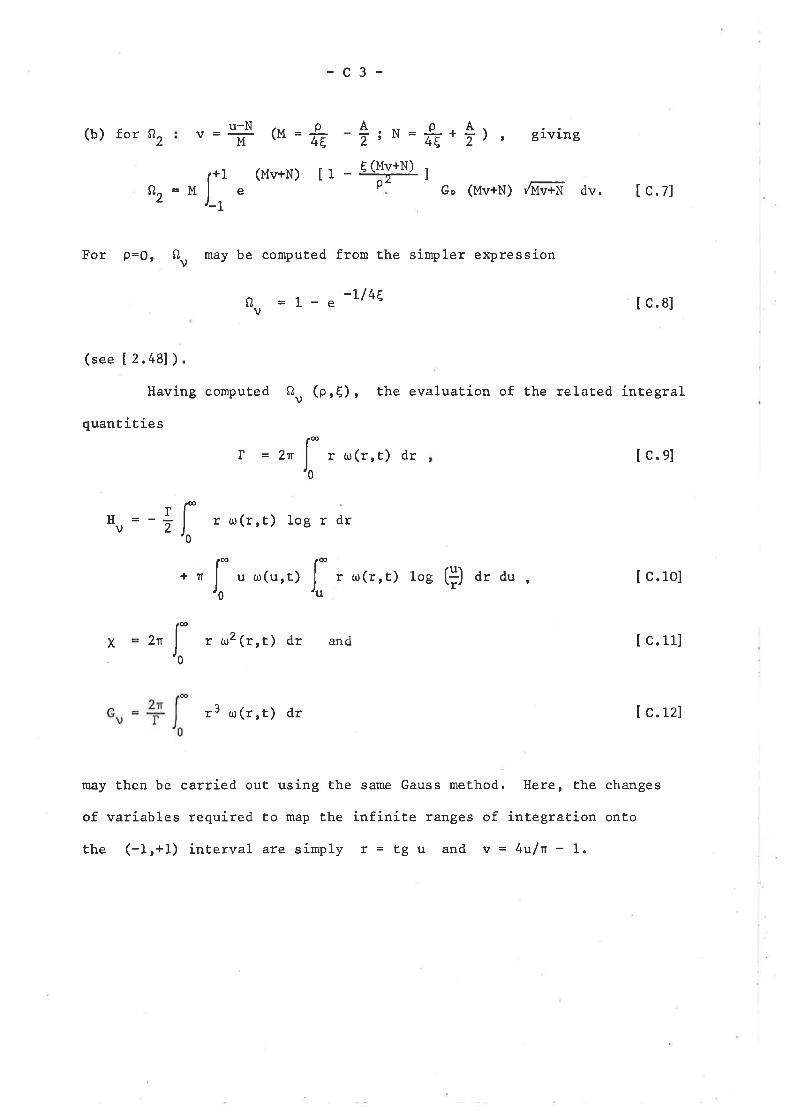
-c3-

(M=å ;N= I *A\ -;.'æ*Z), glvlng

az ti(Mv+N) tr - g(Yl+N)

,=![ e

0v

(see [ 2,481).

Having computed Ou

quantities

| =2n

Go (Mv+w) 'Æ;iN dv. t c. 7l

I c.s¡

(pr€), the evaluation of the related integral

(b) f.or Q,

"u=-åf-'o

u-Nt=-F A2

For p=0, Ou may be computed from the simpler expression

=1-e -u 4E

I r ur (r, t) dr lc.el

r rrr(r,t) log r dr

f J- ' ,{',t) tos (=J dr du ,+Îf u ul (u, t) I c.10]

2r r ur2(rrt) dr and Ic.n]

13 ur(r,t) dr I c. rz]

may then be carried out using the same Gauss method. Here, the changes

of variables required Ëo map Èhe infinite ranges of integration onto

the (-1r+1) interval are simply r = tg u and v = 4t/n - L.

]:X

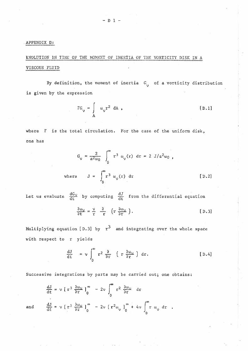
-D1-

APPENDIX D:

EVOLUTION IN TIME OF THE MOMENT OF INERTIA OF THE VORTICITY DISK IN A

VISCOUS FLUID

By definition, Èhe moment of ínertia Gu of a vorticity distríbution

ís given by the expression

,our2 dA ,"=fATG

where I is the total circulaÈion. For the case of the uniform disk,

one has

Io.r]

It.z]

tD.3l

I o.+]

Gv 13 r,rr(r) dr = 2 J/a2ug ,fwhere J =

&dr by courputíng from the differential equation

fr 3 uru (r) dr

Let us evaluate dJãT

-ll¿ar ('þ).vâtt

Multiplying equaËion IO.3] by 13 and integrating over the whole space

with respect to r yields

t2

x2

( r ?t., )dr. dr.

Successive integraÈions by parts may be carried out,¡ one obËains:

dJãE =v["*P]; 2v -4.\¿âr dr

ârfvdJæ

fI- 2v [r2ou J- + 4vS = u r:, åP lr-

a

and r ou dr

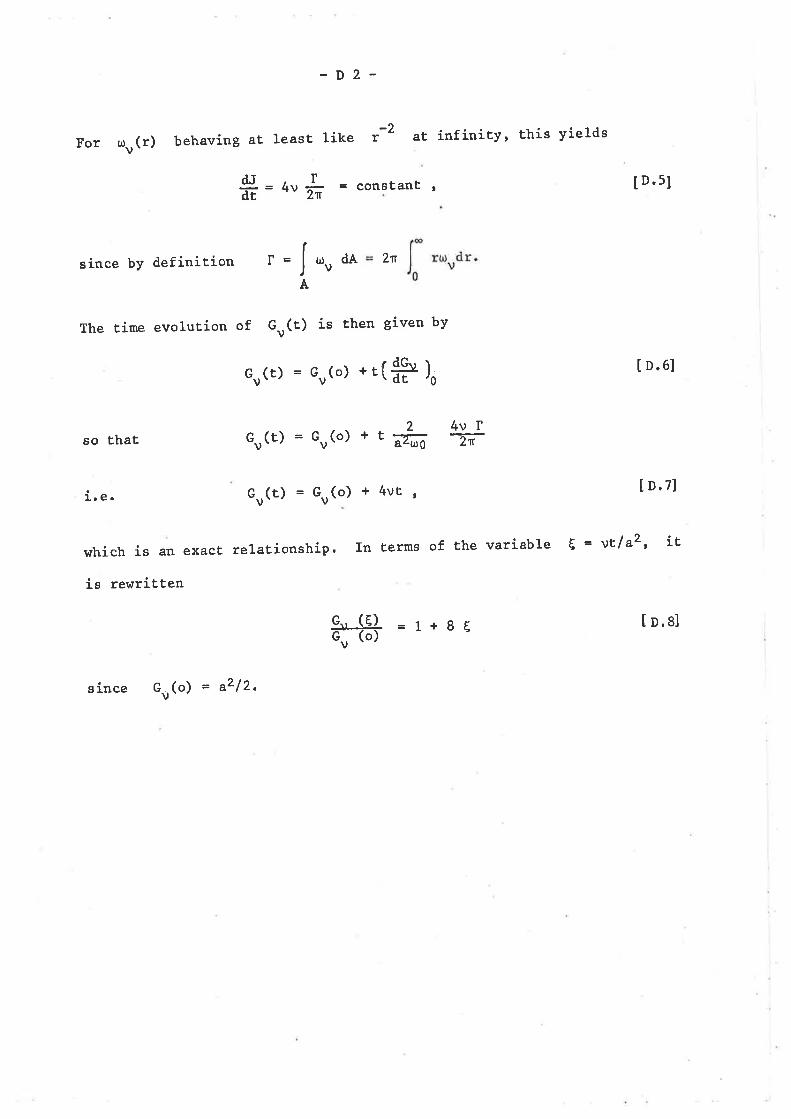
For

since by definition

so that

1. ê.

-D2-

Gv(t) = Gr(o) + 4vt '

tru(r) behaving at least like ;2 at infinity' t'his yields

dJãE =4v ñ = consËant ¡

r

2r¡dAItvr=lA

I D.5]

I D.6]

lo.zl

[¡.e]

The time evolut.ion of Gv(t) is then given by

cv(È) = Gu(o) ..(åP )o

cv(t)=Gu(o) *ET+i 4vIT

which is an exact relationship. In Lerms of the variable E = vtla2' it

is rewritten

c., (t){õ)-

=1+8t

gr-nce co(o) = a212,