Sensory and Motor Systems

The Largest Response Component in the MotorCortex Reflects Movement Timing but NotMovement Type

Matthew T. Kaufman,1,2,5 Jeffrey S. Seely,6 David Sussillo,1,2 Stephen I. Ryu,2,8 Krishna V.Shenoy,1,2,3,4,9 and Mark M. Churchland6,7

DOI:http://dx.doi.org/10.1523/ENEURO.0085-16.2016

1Neurosciences Program, Stanford University, Stanford, California 94305, 2Department of Electrical Engineering,Stanford University, Stanford, California 94305, 3Department of Bioengineering, Stanford University, Stanford,California 94305, 4Department of Neurobiology, Stanford University, Stanford, California 94305, 5Cold Spring HarborLaboratory, Cold Spring Harbor, New York 11724, 6Department of Neuroscience, 7Grossman Center for the Statisticsof Mind, David Mahoney Center for Brain and Behavior Research, Kavli Institute for Brain Science, ColumbiaUniversity Medical Center, New York, NY 10032, 8Department of Neurosurgery, Palo Alto Medical Foundation, PaloAlto, California 94301, and 9Howard Hughes Medical Institute, Stanford University, Stanford, California 94305

Abstract

Neural activity in monkey motor cortex (M1) and dorsal premotor cortex (PMd) can reflect a chosen movement well beforethat movement begins. The pattern of neural activity then changes profoundly just before movement onset. We consideredthe prediction, derived from formal considerations, that the transition from preparation to movement might be accompaniedby a large overall change in the neural state that reflects when movement is made rather than which movement is made.Specifically, we examined “components” of the population response: time-varying patterns of activity from which eachneuron’s response is approximately composed. Amid the response complexity of individual M1 and PMd neurons, weidentified robust response components that were “condition-invariant”: their magnitude and time course were nearlyidentical regardless of reach direction or path. These condition-invariant response components occupied dimensionsorthogonal to those occupied by the “tuned” response components. The largest condition-invariant component was muchlarger than any of the tuned components; i.e., it explained more of the structure in individual-neuron responses. Thiscondition-invariant response component underwent a rapid change before movement onset. The timing of that changepredicted most of the trial-by-trial variance in reaction time. Thus, although individual M1 and PMd neurons essentiallyalways reflected which movement was made, the largest component of the population response reflected movement timingrather than movement type.

Key words: condition-invariant signal; dPCA; movement initiation; movement triggering; reaction time; statespace

Significance Statement

The activity of neurons often conveys information about externally observable variables, such as the location ofa nearby object or the direction of a reach made to that object. Yet neural signals can also relate to “internal”factors: the thoughts and computations that link perception to action. We characterized a neural signal thatoccurs during the transition from preparing a reaching movement to actually reaching. This neural signal conveysremarkably accurate information about when the reach will occur, but carries essentially no information aboutwhat that reach will be. The identity of the reach itself is carried by other signals. Thus, the brain appears toemploy distinct signals to convey what should be done and when it should be done.

New Research

July/August 2016, 3(4) e0085-16.2016 1–25

IntroductionThe responses of individual neurons are often character-ized in terms of tuning: how the firing rate varies acrossdifferent stimuli or behaviors (“conditions”). Additionally,neural responses may contain untuned features that areshared across many conditions, such as an abrupt rise infiring rate after the onset of any stimulus. These untunedresponse features may appear nonspecific, and thus ofsecondary interest. However, there is evidence that re-sponse features can be correlated across conditions, yetstill carry computationally relevant information. Neural ac-tivity in the prefrontal cortex contains a large responsecomponent reflecting the passage of time (Machens et al.,2010), and time-varying signals have also been observedin the premotor cortex during anticipation of an informa-tive cue (Confais et al., 2012). A related example is thetime-encoding urgency signal observed during decisionmaking, which is shared across neurons that encodedifferent choices in both the oculomotor system (Church-land et al., 2008; Hanks et al., 2011) and the premotorcortex (Thura et al., 2012). Here we investigate anotherpossible “untuned” signal in the motor/premotor cortex:one that arises after the desired target is known, at thetime of the sudden transition from preparation to move-ment.

We were motivated by the observation that motor cortexneurons sometimes display broadly tuned movement-period responses (Fortier et al., 1993; Crammond andKalaska, 2000)—e.g., a rise in rate for all directions—suchthat tuning models benefit from an omnidirectional term(Georgopoulos et al., 1986; Moran and Schwartz, 1999).More generally, many studies identify significant proportionsof neurons with responses that are task-modulated yet notstrongly selective for the parameter being examined(Evarts, 1968; Weinrich et al., 1984; Hocherman and Wise,

1991; Riehle et al., 1994; Messier and Kalaska, 2000).These findings argue that there must be some aspect ofneural responses—i.e., some response “component”—that is at least moderately correlated across conditions.What are the temporal properties of such a signal and isits timing predictive of behavior? Does the signal make asmall or large contribution to the overall population re-sponse? Is the signal merely correlated across conditions(“condition-correlated”)? Or might it be nearly identicalacross conditions (“condition-invariant”) and thus un-tuned in the traditional sense?

These questions derive both from a general desire tofully characterize the response during movement andfrom specific theoretical considerations. A condition-invariant signal (CIS) could, despite its seeming lack ofspecificity, be important to the overall computation per-formed by the population. Presumably there is a largechange in computation just before movement onset, atthe moment when the motor system transitions from pre-paring to move while holding a posture (Kurtzer et al.,2005) to generating the muscle activity that will drive thedesired movement. Consistent with the idea of a changein computation, neural tuning changes suddenly and dra-matically at a point �150 ms before movement (Church-land et al., 2010) so that a neuron’s “preference” duringmovement can be quite unrelated to its preference duringpreparation (Wise et al., 1986; Crammond and Kalaska,2000; Kaufman et al., 2010). A similar transition is ob-served at the population level: population dynamics arerelatively stable and attractor-like during preparation butbecome strongly rotational just before movement onset(Churchland et al., 2012). This sudden change in networkproperties is presumably driven by an appropriately timedinput (which could itself be the output of a computationthat decides when to move; Romo and Schultz, 1987;Thaler et al., 1988; Schurger et al., 2012; Murakami andMainen, 2015). One might initially expect a “triggering”input to be tuned (Johnson et al., 1999; Erlhagen andSchöner, 2002). Yet theoretical considerations suggestthat a simple, condition-invariant change in input is suffi-cient to trigger large changes in network dynamics andtuning (Hennequin et al., 2014). In particular, a recentneural network model of motor cortex (Sussillo et al.,2015) uses a condition-invariant input to trigger a changein dynamics that initiates movement. The model’spopulation-level responses resemble the empirical neuralresponses, and from inspection both clearly show at leastsome features that are invariant across conditions.

Critically, there are many ways in which activity patternscan be correlated across conditions. Only a minority ofsuch possibilities involve a true CIS at the populationlevel: that is, a signal that is nearly identical across con-ditions. Is a CIS present in motor cortex? On a trial-by-trialbasis, does it exhibit timing locked to target onset, the gocue, or movement onset? Only the latter would be con-sistent with the role in movement triggering suggested bythe model of Sussillo et al. (2015).

We found that a CIS was not only present but was thelargest aspect of the motor cortex response—consider-ably larger than any of the condition-specific (tuned) re-

Received April 18, 2016; revised July 31, 2016; accepted August 1, 2016; Firstpublished August 3, 2016.The authors report no conflict of interest.Author contributions: M.T.K., K.V.S., and M.M.C. designed research; M.T.K.

and M.M.C. performed research; M.T.K. analyzed data; M.T.K. and M.M.C.wrote the paper; J.S.S., D.S., and S.R. contributed unpublished reagents/analytic tools.

This work was supported by the Grossman Charitable Trust, National Sci-ence Foundation graduate research fellowships (M.T.K., J.S.S.), a SwartzFoundation fellowship (M.T.K.), Burroughs Wellcome Fund Career Awards inthe Biomedical Sciences (M.M.C., K.V.S.), National Institutes of Health (NIH)Director’s Pioneer Award 1DP1OD006409 (K.V.S.), Defense Advanced Re-search Projects Agency Reorganization and Plasticity to Accelerate InjuryRecovery N66001-10-C-2010 (K.V.S.), NIH Director’s New Innovator Award(M.M.C.), Searle Scholars Award (M.M.C.), Sloan Research Fellowship(M.M.C.), McKnight Scholar Award (M.M.C.), a Klingenstein-Simons Fellow-ship Award (M.M.C.), and the Simons Foundation (M.M.C., M.T.K.). We thankW. Brendel for dPCA code and advice, M. Mazariegos for expert surgicalassistance and veterinary care, and D. Haven and B. Oskotsky for technicalsupport.

Correspondence should be addressed to Mark Churchland, Kolb Re-search Annex, 40 Haven Avenue, New York, NY 10032-2652. E-mail:mc3502@columbia.edu

DOI:http://dx.doi.org/10.1523/ENEURO.0085-16.2016Copyright © 2016 Kaufman et al.This is an open-access article distributed under the terms of the CreativeCommons Attribution 4.0 International, which permits unrestricted use, distri-bution and reproduction in any medium provided that the original work isproperly attributed.

New Research 2 of 25

July/August 2016, 3(4) e0085-16.2016 eNeuro.org

sponse components. The CIS resembled the previouslyreported omnidirectional or “speed-tuned” responsecomponent (Georgopoulos et al., 1986; Moran andSchwartz, 1999), but was essentially invariant with reachspeed, distance, and curvature. In addition, the CIS un-derwent a large and sudden change �150 ms beforemovement onset. The timing of this change was an ex-cellent predictor of reaction time (RT) on a trial-by-trialbasis. Finally, the dimensions in neural state space thatwere occupied by the CIS were almost perfectly orthog-onal to the dimensions occupied by the condition-specificcomponents. Overall, the profile, timing, and population-level manifestation of the CIS were remarkably similar tothe structure naturally produced by the model of Sussilloet al. (2015). Our findings thus suggest a potential role fora large response component that initially appears nonspe-cific yet reflects movement timing very precisely.

Materials and MethodsThe key features of the task and analyses are described inthe Results. Below we detail all aspects of the apparatus,task, neural recordings, muscle recordings, data prepro-cessing, analyses, and controls.

Subjects and taskAnimal protocols were approved by the Stanford Univer-sity Institutional Animal Care and Use Committee. Exper-iments employed two adult male rhesus monkeys(Macaca mulatta), J and N, performing a delayed-reachtask on a frontoparallel screen (Churchland et al., 2010,2012; Kaufman et al., 2013). The monkey initially fixated acentral spot with his eyes and touched it with a cursor.The cursor was projected slightly above the right fingertip,which was tracked optically. The task involved a largenumber of conditions—i.e., different target locations andreach paths—which was useful when attempting to iden-tify response components that are invariant across con-ditions. On one-third of trials (“no-barrier” conditions) alone target appeared within a frame around the work-space. On another one-third of trials (“maze” conditions) atarget and �9 virtual barriers appeared. The remainingone-third of trials (“maze-with-distractor” conditions)were identical to the maze trials but included two distrac-tor “targets” that were unreachable due to the barrierlocations. The same set of target positions was used forthe no-barrier, maze, and maze-with-distractor condi-tions. When barriers were present, the monkey had toperform a curved reach or the cursor would collide withand “stick” to the barrier. This paradigm evoked bothstraight and curved reaches in different directions and ofvarying speed and distance. Most datasets employed 27conditions (nine of each type) while one (NAC) employed108. No attempt was made to produce a uniform arrange-ment of target locations or initial reach directions, but wenote that all datasets involved reaches that spanned thespace of directions in two-dimensional space, and thatresults were consistent across the different datasets,which typically employed different arrangements of tar-gets and barriers. More broadly, the large variety of con-ditions we employed provides a stringent test regardingwhether a signal is truly condition-invariant.

A randomized delay period separated target onset froma go cue. During the delay, targets jittered slightly (2–3mm), indicating to the monkey that he could not yet reachor saccade. The go cue consisted of three simultaneousand salient cues: jitter ceasing, the targets changing fromopen to filled, and the central spot disappearing. Juicereward was delivered if the monkey swiftly reached to thetarget then held it for 450 ms (monkey J) or 700 ms(monkey N).

Delay-period statisticsThe delay period lasted 0-1000 ms. Different datasetsemployed different delay-period statistics, depending onthe analyses we wished to apply. Three datasets (JC,NAC, and NS) were collected with the primary goal ofanalyzing trials with longer delays. Longer delays enabledexamination of the transition between a relatively stableplateau of preparatory activity and subsequent movement-related activity. To this end, delays of 450-1000 ms wereapproximately twice as probable as delays of 0-450 ms.Three further datasets (JAD1, JAD2, NAD) were recordedwith the goal of characterizing the single-trial relationshipbetween neural activity and response time (RT). For thesedatasets, delay durations of 0, 100, 200, and 500 ms wereintentionally over-represented. These dataset names endwith “D,” indicating that this set of discrete delays wasover-represented. This allowed key analyses to be re-stricted to a set of trials with the same delay, removing thepotential confound that RT can vary with delay. For thesedatasets most trials (78, 78, and 84% for datasets JAD1,JAD2, and NAD) used one of the discrete delays, withroughly equal probability. The remaining trials had ran-dom delays from 0 to 1000 ms as above. Because thesedatasets were each collected in a single day using im-planted multielectrode arrays, the monkeys were not an-ticipating the over-represented delay durations.

Most analyses focused on the transition from move-ment preparation to movement and thus used only trialswith �450 ms delays (datasets without discrete delays) or500 ms delays (datasets with discrete delays). For analy-ses of the single-trial relationship with RT, we focused ondatasets with discrete delay durations. For simplicity ofpresentation, for these analyses only trials with no delay(“zero delay”) or a 500 ms delay (“long delay”) are shown.All results were similar for delays of 100 or 200 ms.

Catch trials and trial countsSeveral types of unanalyzed catch trials ensured the taskwas performed as desired. In particular, we presentednovel mazes made by randomly removing barriers from astandard maze (10–15% of all trials), or randomly placingthe target and two barriers (0–10% of all trials). Thesetrials ensured that the monkey had to solve each trialindependently, as similar-looking mazes could have dif-ferent solutions.

Delay periods were randomly chosen on each trial.Conditions were organized in pseudorandom blocks. Thearray datasets had 3352, 2340, 2622, and 3590 success-ful trials (datasets JAD1, JAD2, NAD, and NAC) from asingle session. For the “discrete delay” datasets (JAD1,JAD2, and NAD) there were �250–500 usable trials for

New Research 3 of 25

July/August 2016, 3(4) e0085-16.2016 eNeuro.org

each of the four over-represented delays. Usable trialsexcluded catch trials, failed trials (e.g., if a barrier werestruck), rare trials with an unusual velocity profile that didnot allow a reliable RT measurement, and trials with a veryshort RT (in rare instances where the monkey “jumped thegun”) or an overly long RT (in rare instances where themonkey was presumably distracted). Datasets that in-cluded single-unit recordings (JC and NS) contained anaverage of 336 and 305 usable trials per unit.

Neural and muscle recordingsFor both monkeys, we first performed single-electroderecordings (datasets JC and NS) using moveable tung-sten microelectrodes (Frederick Haer) and a PlexonMultichannel Acquisition Processor (Plexon). These re-cordings included the caudal portion of the dorsal premo-tor cortex (PMd) and both surface and sulcal primarymotor cortex (M1). All units recorded with single elec-trodes were well-isolated single neurons recorded fromregions where microstimulation produced movement ofthe arm (typically the upper arm and/or shoulder). Eachmonkey was then implanted with two 96-electrode siliconarrays (Blackrock Microsystems), located in M1 and cau-dal PMd, as estimated from anatomical landmarks andprevious mapping with microstimulation. Spikes weresorted off-line using custom software (MKsort, https://github.com/ripple-neuro/mksort). For array recordings,both single units and stable multiunit isolations (typicallytwo neurons whose spikes could not be reliably sepa-rated) were analyzed. A strong CIS (see below) was pres-ent regardless of whether a dataset involved pure single-unit isolations or a mixture of single-unit and multiunitisolations. This is unsurprising: dimensionality reductiontechniques, such as demixed principal component anal-ysis (dPCA) or PCA, typically produce nearly identicalresults regardless of whether isolations involve one unit ora few units. These techniques are forgiving because thecomponents needed to compose the responses of a sin-gle neuron are the same components needed to composethe summed response of �1 neuron. All neural recordingswere from the left hemisphere. Array recordings produceddatasets JAD1, JAD2, NAD, and NAC, and were includedin dataset JC.

We analyzed all units where the firing rate range (overconditions and times) was greater than the maximal SEM(for all conditions and times). This signal-to-noise (SNR)criterion does not insist on any particular form of responseor tuning—only that there be some response. For datasetJAD1, 116 of 123 units passed the SNR criterion; fordataset JAD2, 136 of 171 units passed; for dataset JC,186 of 278 units passed; for dataset NAD, 172 of 188 unitspassed; for dataset NAC, 213 of 223 units passed; fordataset NS, 118 of 118 units passed. Of these, 67, 28,108, 62, 58, and 118 were considered single units (data-sets JAD1, JAD2, JC, NAD, NAC, and NS). For all analy-ses, results were similar when data from PMd and M1were analyzed separately. These recordings were there-fore pooled.

Data preprocessing involved three steps. First, spiketrains were smoothed with a Gaussian (28 ms SD). Sec-

ond, the firing rate was averaged across trials of the sametype (excepting analyses of single trials; see below). Wecomputed two averages: one with data aligned to targetonset and one with data aligned to movement onset.Third, the firing rate of each neuron was normalized toprevent analyses from being dominated by a few high-rateneurons; this is especially important (Yu et al., 2009) whenperforming PCA-based analyses. To normalize withoutoveramplifying the greater noise associated with low firingrates, we “soft normalized”: for each neuron we normal-ized the firing rate by its range (across all times andconditions) plus a constant, chosen to be 5 spikes/s. Thischoice follows our previous work, and was made beforeperforming analyses. Results were extremely similar andsometimes stronger if we used a soft-normalization con-stant of zero.

Electromyographic (EMG) recordings used hook-wireelectrodes (44 gauge with a 27 gauge cannula; NicoletBiomedical), inserted percutaneously into the muscles ofthe right arm. Electrodes were inserted with the monkeyawake and calm, with one recording per session. Formonkey J, recordings were made sequentially from tra-pezius, latissimus dorsi, pectoralis, triceps brachii, medialand lateral aspects of the biceps brachii, and anterior,medial, and posterior aspects of the deltoid. The record-ing from the triceps was excluded because it was notsufficiently modulated during the task. For monkey N,recordings were made from proximal, middle, and distalaspects of the trapezius, latissimus dorsi, pectoralis, tri-ceps brachii, medial and lateral aspects of the biceps, andanterior, medial, and posterior aspects of the deltoid. Tworecordings were made for each deltoid site. The record-ings from the triceps and latissimus dorsi were excludedbecause they were not sufficiently modulated during thetask. Raw EMG signals were band-pass filtered (150–500Hz, four pole, 24 db/octave), differentiated, rectified,smoothed with a Gaussian (15 ms SD), and averagedacross trials (Kaufman et al., 2013).

Projections of neural dataWe identified response components by projecting thepopulation response onto dimensions of interest. We be-gan with a matrix, R, of trial-averaged neural responses(or EMG, for one analysis). Each of n columns containedthe normalized response of one neuron over time, withresponses concatenated across conditions. To projectthe data onto a given dimension we computed xh � Rwh,where wh is a set of weights specifying the dimension. Theprojection xh is therefore a weighted average of neurons’firing rates. We refer to the projected activity pattern as a“component” of the population response, because theactivity of any given neuron can be (approximately) com-posed of a weighted sum of multiple such components.This use of the term “component” follows the usage ofKobak et al. (2016) and others. Note that this use of“component” is not synonymous with “principal compo-nent,” which refers to a component of the neural covari-ance matrix and thus corresponds to a neural dimension.

Many studies have been concerned with how to bestfind projections given different goals and hypotheses. In

New Research 4 of 25

July/August 2016, 3(4) e0085-16.2016 eNeuro.org

this study the most important projection method usesdPCA (Machens et al., 2010; Brendel et al., 2011) to findthe dimensions wh. This application of dPCA is detailedmore thoroughly in the next section.

We also use a number of other projection methods,including standard PCA, and simply computing the meanacross neurons (equivalent to setting all weights to 1/n).Two analyses use the jPCA method (Churchland et al.,2012), and in one case we used a classifier trained via asupervised algorithm. In every case it should be stressedthat the projections shown (i.e., the response compo-nents) are simply linear weightings of the recorded neuralresponses. The use of multiple methods is desirable be-cause no single method can capture all aspects of theresponse (e.g., the mean captures some aspects of theresponse and hides others).

All projection methods used here employ orthonormaldimensions. The orthogonality of these dimensions doesnot impose orthogonality on aspects of the neural re-sponse; it is simply a way of choosing a coordinate sys-tem. An orthonormal basis makes interpretation simpler:among other benefits, it allows each component to beindependently quantified in terms of variance explained,making it harder to unintentionally interpret weak struc-ture as meaningful. In all cases, when a percentage ofvariance is quoted, it is the fraction of the variance cap-tured in the low-dimensional space (10–12 dimensions).

Identifying the CIS via dPCAMany of our central analyses sought to determine whetherthere exist neural dimensions that segregate condition-specific (“tuned”) components from condition-invariantcomponents of the population response. By “condition-specific” we mean that different conditions (reach direc-tions, curvatures, etc.) evoke different responses whenthe population response is projected onto that dimension.

By “condition-invariant” we mean that the responsevaries with time but is similar across conditions whenprojected onto that dimension. To address this question,we applied dPCA (Machens et al., 2010; Brendel et al.,2011), a variant of PCA. dPCA leverages information nor-mally discarded by PCA: each row of the data matrix R isassigned labels. Here, those labels indicated the condi-tion and time for which that set of firing rates was re-corded. dPCA then finds a matrix W that produces aprojection X of the data R, with X � RW. Each column ofW is a dimension and each column of X is a component ofthe population response. Like PCA, dPCA attempts to finda projection that captures much of the variance in R, sothat R � XWT. Unlike PCA, dPCA attempts to find W suchthat the resulting columns of X covary strongly with onelabel or the other. In the present case, dPCA attempts tofind W such that some columns of X (some components)vary with time but not condition and other columns varyacross conditions but not with time. As will be discussedbelow, such segregation is not necessarily possible: ingeneral there will not exist a W with the desired properties.Indeed, in the present study, dPCA always found compo-nents that varied primarily with time (and not condition)but never found components that varied primarily with

condition and not time. We therefore divided the compo-nents found by dPCA into two groups: condition-invariant(reflecting primarily time) and condition-specific (reflectingboth condition and time). We refer to the group ofcondition-invariant components collectively as the CIS.

As a technical note, dPCA (unlike PCA) requires that thenumber of dimensions be specified in advance. Prioranalyses indicate that 6–8 dimensions capture much ofthe condition-specific structure of the data (Churchlandet al., 2010). We therefore wished that dPCA should cap-ture a similar amount of condition-specific structure, inaddition to any condition-invariant structure that might bepresent. We empirically picked the number of requesteddimensions such that dPCA returned eight condition-specific dimensions (defined as containing �50% condition-invariant variance). In principle this might have necessitatedrequesting exactly eight dimensions (if all structurewere tuned) or many more than eight (if little structurewere tuned). In practice it was only necessary to re-quest modestly more than eight total dimensions. Forexample, for dataset JAD1 we requested 10 total dimen-sions, which yielded two condition-invariant responsecomponents and eight condition-specific response com-ponents. The choice of eight condition-specific compo-nents is an arbitrary but reasonable cutoff. We alwaysfound a strong CIS regardless of the exact number ofdimensions requested. dPCA identified dimensions (W)based on the population response from �200 to �400 msrelative to target onset and �300 to �600 ms relative tomovement onset. The data matrix being analyzed con-tained trial-averaged firing rates for long-delay trials (trialswith delay periods �450 ms). For subsequent analyses oftrial-to-trial variability in RT, we projected data from indi-vidual trials, including zero-delay trials, onto the samedimensions. The probabilistic-model version of dPCA wasused (from the Python code available online associatedwith Brendel et al., 2011). We measured for each re-sponse component the marginal variances (Machenset al., 2010; Brendel et al., 2011), which indicate howmuch of a component’s variance was condition-specific(activity varying with condition or with both time andcondition) versus condition-invariant (activity varying withtime alone).

Because EMG responses were lower dimensional thanneural responses, for the EMG datasets dPCA was per-formed at an overall dimensionality that returned threecondition-specific dimensions. The resulting 4–5 dimen-sions (monkey J, N) accounted for 95–97% of the totalvariance in the EMG data. This reduced number of dimen-sions did not produce the differences between neural andmuscle data: repeating the analysis on neural data using4–5 dimensions yielded essentially identical results tothose obtained with more dimensions.

Note regarding interpretation of the segregationproduced via dPCABelow we describe a key interpretational point regardingthe dPCA method. The cost function optimized by dPCAattempts to find W such that each column of X (eachresponse component) varies with exactly one of the pro-

New Research 5 of 25

July/August 2016, 3(4) e0085-16.2016 eNeuro.org

vided labels (time and condition in this study) and not withthe other(s). Yet as stated above, this segregation is not ingeneral possible. In the present case, this has two impli-cations. First, it is not guaranteed that dPCA will be ableto find components that vary with condition but not withtime; perhaps every component that strongly reflects con-dition also reflects time (this was indeed true of our data).Second, it is similarly not guaranteed that dPCA will beable to find components that vary with time but not con-dition; it may be that every component that strongly re-flects time also reflects condition.

This last fact is worth stressing because many individ-ual neurons exhibit what we refer to as “condition-correlated” structure: responses that are different acrossconditions, yet display an increase (or decrease) in firingrate that has a somewhat similar time course acrossconditions. Yet this structure at the single-neuron level isnot sufficient, in and of itself, to indicate condition-invariantstructure at the population level. Would dPCA, when appliedto a population of such neurons, inevitably find condition-invariant components? In short, it would not. This can bedemonstrated empirically (see Results) or formally via con-struction, as follows. Consider a simple case in which eachneuron’s response rn is a linear combination of two indepen-dent components xi (which will also be functions of conditionc and time t): rn, c, t � �

i�1:2wn, i x i, c, t. Let both x1, c, t and x2, c, t be

condition-specific, but suppose x1, c, t contains an overallcorrelation between conditions. Due to the correlation ofx1, c, t across conditions, the responses r will also haveshared response features across conditions. Nevertheless, itis not in general possible to find a linear combination of thern, c, t’s that is condition-invariant. A linear combination of thern, c, t’s is equivalent to a linear combination of x1, c, t and x2, c, t.Since these components are independent, finding acondition-invariant linear combination is equivalent to solv-ing the following system of �C � 1�T equations, where C isthe number of conditions (here, 2), and T is the number oftime points:

�i�1:2

pixi,c,t � �i�1:2

pixi,c�1,t

for all times t and all pairs of conditions c and c � 1 (thisis a sufficient constraint to ensure that all pairs of condi-tions are equal, since equality is transitive).

The number of free variables pi is equal to the numberof components D, which in this example is 2. In general,then, this system is not solvable if �C � 1�T � D, whichwill be true for even modest numbers of times and con-ditions. The presence of correlated structure within x1, c, t

(and/or x2, c, t) would not in general change this fact. Inpractice, then, it would be rare for condition-correlatedresponses to coincidentally produce a fully condition-invariant component. As one example, choose x1, c, t �gcsin�t� and x2, c, t � hcsin�3t�, with gc and hc being positivescalars that vary with condition. Both x1, c, t and x2, c, t

would be perfectly condition-correlated, yet no linearcombination of x1, c, t and x2, c, t would be condition-invariant.

Control: producing synthetic peristimulus timehistograms with matched spectral contentTo illustrate empirically that condition-invariant compo-nents are not found in “generic” data, we generated syn-thetic peristimulus time histograms (PSTHs) with thesame frequency content as the original neurons. Each unitwas matched with a corresponding synthetic PSTH. Thesteps below were performed on the vector containing thetrial-averaged firing rate over time for one condition. Wefirst preprocessed each vector by smoothing lightly (10ms SD Gaussian) to reduce the small discontinuity be-tween target-aligned and movement-aligned data, thenmultiplying by a Hann window. The Fourier transform wasperformed, and the magnitude of the result was com-puted at each frequency (i.e., the square root of powerspectral density). These curves were averaged over con-ditions to give the overall power-by-frequency curve forthat unit. To construct a synthetic PSTH for each condi-tion, we chose a random phase for each frequency com-ponent, then took the inverse Fourier transform.

Control: removing the CIS from the neural responsesTo ask whether condition-invariant components (collec-tively the CIS) might result from the rectification of firingrates at zero, we removed the true condition-invariantcomponents, rerectified firing rates, then applied dPCA.Specifically, we projected the population response ontothe eight condition-specific dimensions identified bydPCA, then transformed the data back to the originaln-dimensional space. This produced as many PSTHs asthe original neurons. We rescaled and recentered each“neuron’s” response to restore its original mean andrange of firing rates. Finally, we set all negative firing ratesto zero. This resulted in a population of surrogate neuronsthat are responsive and have positive firing rates, yetshould have no “true” CIS. Thus, a strong CIS in thiscontrol population would indicate that rectified firing ratescould create an artifactual CIS.

Control: adding a condition-correlated componentWe constructed additional surrogate data that resembledthe empirical data but lacked condition-invariant compo-nents. For each empirical condition-invariant component,we constructed a new component with the same timecourse, but with varying amplitude across conditions.That is, we created components that were condition-correlated but not condition-invariant. These componentswere recentered to have a zero mean during the baselineperiod (before target/maze onset), and then were addedto the response of each neuron. Specifically, to eachneuron’s response rn,c,t we added wn,i kcx’i,t, where wn,i is

the neuron’s original weight for the ith condition-invariantcomponent, x’i,t is the time course of the ith new condition-correlated component, and the coefficients kc were cho-sen randomly from a unit-variance Gaussian distribution.We rectified the resulting firing rates (setting all negativerates to zero). These operations largely preserved the timecourse of each neuron’s across-condition mean (becausethe kc’s were zero-mean). Because the new componentswere condition-correlated, the responses of most neurons

New Research 6 of 25

July/August 2016, 3(4) e0085-16.2016 eNeuro.org

were strongly condition-correlated. Yet because the orig-inal condition-invariant components are now “contami-nated” with condition-specific components of the sametime course, the surrogate population should have noseparable condition-invariant components.

Identifying a speed-predicting dimensionTo identify a speed-predicting dimension, we began withthe same neural data matrix R used for PCA and dPCA.We then regressed the trial-averaged speed profile foreach condition against R: sh � Rwh � b, where sh is thevector produced by taking the speed profile for eachcondition and concatenating the conditions, b is the bias(a constant offset), and wh specifies a set of weights. Thespeed profile was advanced by 150 ms before regressionto accommodate known lags.

Trial-by-trial analysisTo assess how well projections onto different dimensionspredict trial-by-trial movement onset we performed foursteps: (1) we chose a potentially informative weightedsum of neurons (“dimension of interest”); (2) we binnedand smoothed the spiking data on individual trials; (3) weprojected the population neural response from each trialonto the dimension of interest; and (4) for each trial wefound the time point at which that projection exceeded acriterion value. That time, relative to the go cue, was thepredicted RT. These steps are explained in more detailbelow.

For the first step, we compared the performance ofseveral different techniques for finding the dimension ofinterest. Three of these techniques were unsupervised:dimensions were identified based on the structure of thedata without exploiting prior knowledge of the RT. Thesethree methods—the CIS1 method, the PC1 method, andthe mean-over-all-neurons method—used dPCA, PCA,and simple averaging, respectively. The CIS1 dimension(producing the largest condition-invariant component)and the PC1 dimension (the largest principal component)were found using the long-delay, trial-averaged data (asabove). We also employed a linear decoder of reachspeed (see above) and a supervised “classifier” method,described below.

For the second step, spikes were counted in 10 msbins, from 60 ms before to 500 ms after the go cue. Eachtrial’s spike counts were convolved with a 30 ms Gaussianto produce a smooth spike rate. For the third step, wecomputed a weighted sum of the neurons’ spike rates.The weights depended on the dimension of interest,found during step one. We refer to the result of this thirdstep as z(t,r), the projection of the neural data as a func-tion of time and trial.

For the final step, we wished to determine when z(t,r)changed in advance of movement onset. To estimate thattime, for each trial we asked when z(t,r) first crossed acriterion value derived from the long-delay trials. To findthat criterion value, we took the median of z(t,r) acrosstrials, producing z̃�t�. We set the criterion value to be themidpoint of z̃�t�: �max �z̃�t�� � min �z̃�t���/2. The midpoint isan arbitrary but reasonable choice to ensure robustness.

For each trial, we found the time at which the criterionvalue was crossed. Trials that never exceeded the crite-rion value, or that exceeded it before the go cue, werediscarded from the analysis. Such trials were uncommon,especially for the better prediction methods (0–9%, de-pending on dataset and method).

The three methods described above—the CIS1 method,the PC1 method, and the mean-over-all-neurons meth-od—predict RT in an unsupervised manner. They werecompared with a supervised method that was allowed touse knowledge of each trial’s RT. This “classifier” methodwas based on logistic regression. Single-trial data werefirst aligned to movement onset, then projected into thedPCA space (including both condition-specific andcondition-invariant dimensions). Data were binned into a“premovement” time point (�360 to �150 ms relative tomovement onset) and a “movement” time point (�150 to�60 ms relative to movement onset). The dividing point of150 ms before movement onset was chosen to approxi-mate the delay between when neural firing rates begin tochange and when the hand begins to move. Logisticregression returned both a projection dimension and acriterion value that best discriminated between the pre-movement and movement data.

As with the other projection methods, the classifierproduces a projection vector wh with as many coefficientsas dimensions of the data (in this case, the number ofcomponents from dPCA). To characterize the classifier,we asked how much each dPCA component contributedto this projection. Specifically, we took the quantity

�whd�·�var��RD�d�, where �whd� is the absolute value of thedth element of wh, D is the dPCA projection matrix (calledW in previous equations), (RD)d indicates the dth columnof the matrix resulting from multiplying RD, and var[ ]indicates taking the variance. This tells us how stronglyeach of the response components (returned by dPCA)contributed to the final classification.

Finally, we used a semisupervised method where RTwas predicted as the time when the decoded reach speedcrossed a 50% threshold. Importantly, for all the abovemethods, training employed only the long-delay data.Trial-by-trial prediction of RT for zero-delay data wasentirely based on generalization. Analyses were based on385/465 trials for dataset JAD1 (long-delay/zero-delay),249/264 trials for dataset JAD2, 260/427 trials for datasetNAD, and 2982 long-delay trials for dataset NAC.

Finding a rotational planeFor some analyses, we wished to identify planes (two-dimensional projections of the population response) con-taining rotational structure. We performed dPCA and thenapplied jPCA (Churchland et al., 2012) to the condition-specific components, using an epoch when neural activityis changing rapidly (�200 to �150 ms relative to move-ment onset). As a technical detail, the PCA step and meansubtraction were disabled in the jPCA algorithm; dPCAserved as a more principled way of focusing jPCA on thestrongly condition-specific dimensions. Because bothdPCA and jPCA produce linear projections, the final resultis also a linear projection of the data.

New Research 7 of 25

July/August 2016, 3(4) e0085-16.2016 eNeuro.org

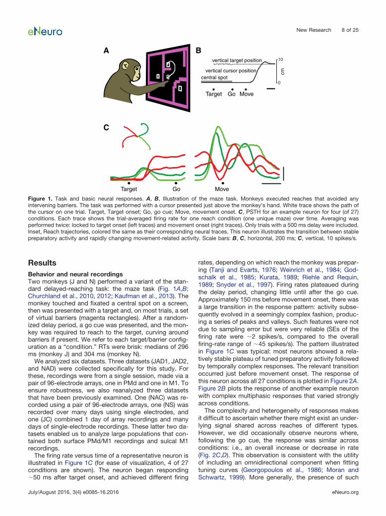
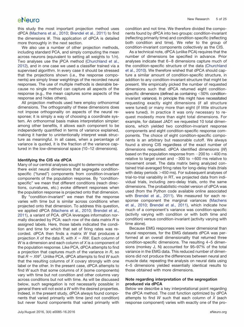
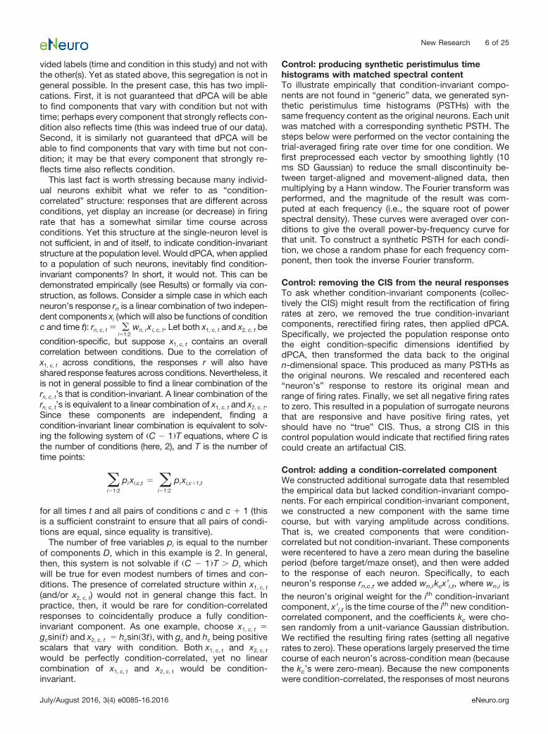
ResultsBehavior and neural recordingsTwo monkeys (J and N) performed a variant of the stan-dard delayed-reaching task: the maze task (Fig. 1A,B;Churchland et al., 2010, 2012; Kaufman et al., 2013). Themonkey touched and fixated a central spot on a screen,then was presented with a target and, on most trials, a setof virtual barriers (magenta rectangles). After a random-ized delay period, a go cue was presented, and the mon-key was required to reach to the target, curving aroundbarriers if present. We refer to each target/barrier config-uration as a “condition.” RTs were brisk: medians of 296ms (monkey J) and 304 ms (monkey N).

We analyzed six datasets. Three datasets (JAD1, JAD2,and NAD) were collected specifically for this study. Forthese, recordings were from a single session, made via apair of 96-electrode arrays, one in PMd and one in M1. Toensure robustness, we also reanalyzed three datasetsthat have been previously examined. One (NAC) was re-corded using a pair of 96-electrode arrays, one (NS) wasrecorded over many days using single electrodes, andone (JC) combined 1 day of array recordings and manydays of single-electrode recordings. These latter two da-tasets enabled us to analyze large populations that con-tained both surface PMd/M1 recordings and sulcal M1recordings.

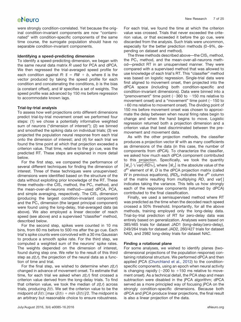
The firing rate versus time of a representative neuron isillustrated in Figure 1C (for ease of visualization, 4 of 27conditions are shown). The neuron began responding�50 ms after target onset, and achieved different firing

rates, depending on which reach the monkey was prepar-ing (Tanji and Evarts, 1976; Weinrich et al., 1984; God-schalk et al., 1985; Kurata, 1989; Riehle and Requin,1989; Snyder et al., 1997). Firing rates plateaued duringthe delay period, changing little until after the go cue.Approximately 150 ms before movement onset, there wasa large transition in the response pattern: activity subse-quently evolved in a seemingly complex fashion, produc-ing a series of peaks and valleys. Such features were notdue to sampling error but were very reliable (SEs of thefiring rate were �2 spikes/s, compared to the overallfiring-rate range of �45 spikes/s). The pattern illustratedin Figure 1C was typical: most neurons showed a rela-tively stable plateau of tuned preparatory activity followedby temporally complex responses. The relevant transitionoccurred just before movement onset. The response ofthis neuron across all 27 conditions is plotted in Figure 2A.Figure 2B plots the response of another example neuronwith complex multiphasic responses that varied stronglyacross conditions.

The complexity and heterogeneity of responses makesit difficult to ascertain whether there might exist an under-lying signal shared across reaches of different types.However, we did occasionally observe neurons where,following the go cue, the response was similar acrossconditions: i.e., an overall increase or decrease in rate(Fig. 2C,D). This observation is consistent with the utilityof including an omnidirectional component when fittingtuning curves (Georgopoulos et al., 1986; Moran andSchwartz, 1999). More generally, the presence of such

0

10

cm

BAvertical target position

vertical cursor positioncentral spot

C

Target Go Move

Target Go Move

Figure 1. Task and basic neural responses. A, B, Illustration of the maze task. Monkeys executed reaches that avoided anyintervening barriers. The task was performed with a cursor presented just above the monkey’s hand. White trace shows the path ofthe cursor on one trial. Target, Target onset; Go, go cue; Move, movement onset. C, PSTH for an example neuron for four (of 27)conditions. Each trace shows the trial-averaged firing rate for one reach condition (one unique maze) over time. Averaging wasperformed twice: locked to target onset (left traces) and movement onset (right traces). Only trials with a 500 ms delay were included.Inset, Reach trajectories, colored the same as their corresponding neural traces. This neuron illustrates the transition between stablepreparatory activity and rapidly changing movement-related activity. Scale bars: B, C, horizontal, 200 ms; C, vertical, 10 spikes/s.

New Research 8 of 25

July/August 2016, 3(4) e0085-16.2016 eNeuro.org

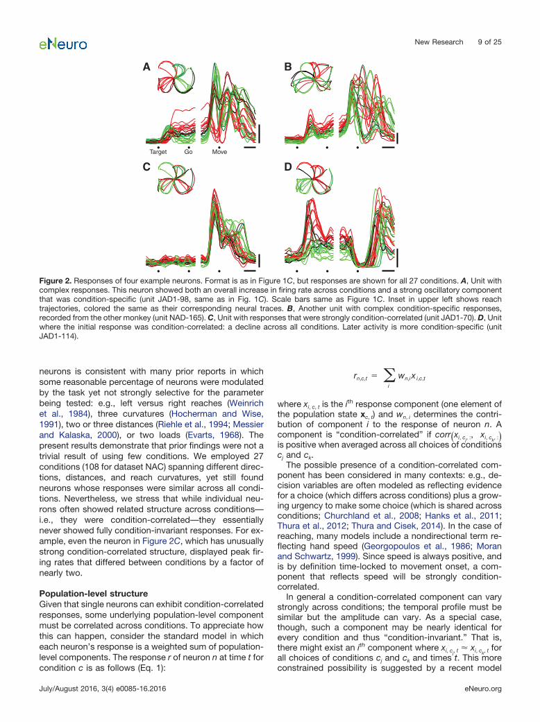
neurons is consistent with many prior reports in whichsome reasonable percentage of neurons were modulatedby the task yet not strongly selective for the parameterbeing tested: e.g., left versus right reaches (Weinrichet al., 1984), three curvatures (Hocherman and Wise,1991), two or three distances (Riehle et al., 1994; Messierand Kalaska, 2000), or two loads (Evarts, 1968). Thepresent results demonstrate that prior findings were not atrivial result of using few conditions. We employed 27conditions (108 for dataset NAC) spanning different direc-tions, distances, and reach curvatures, yet still foundneurons whose responses were similar across all condi-tions. Nevertheless, we stress that while individual neu-rons often showed related structure across conditions—i.e., they were condition-correlated—they essentiallynever showed fully condition-invariant responses. For ex-ample, even the neuron in Figure 2C, which has unusuallystrong condition-correlated structure, displayed peak fir-ing rates that differed between conditions by a factor ofnearly two.

Population-level structureGiven that single neurons can exhibit condition-correlatedresponses, some underlying population-level componentmust be correlated across conditions. To appreciate howthis can happen, consider the standard model in whicheach neuron’s response is a weighted sum of population-level components. The response r of neuron n at time t forcondition c is as follows (Eq. 1):

rn,c,t � �i

wn,i x i,c,t

where xi, c, t is the ith response component (one element ofthe population state xc, t) and wn, i determines the contri-bution of component i to the response of neuron n. Acomponent is “condition-correlated” if corr�xi, cj, :, xi, ck, :�is positive when averaged across all choices of conditionscj and ck.

The possible presence of a condition-correlated com-ponent has been considered in many contexts: e.g., de-cision variables are often modeled as reflecting evidencefor a choice (which differs across conditions) plus a grow-ing urgency to make some choice (which is shared acrossconditions; Churchland et al., 2008; Hanks et al., 2011;Thura et al., 2012; Thura and Cisek, 2014). In the case ofreaching, many models include a nondirectional term re-flecting hand speed (Georgopoulos et al., 1986; Moranand Schwartz, 1999). Since speed is always positive, andis by definition time-locked to movement onset, a com-ponent that reflects speed will be strongly condition-correlated.

In general a condition-correlated component can varystrongly across conditions; the temporal profile must besimilar but the amplitude can vary. As a special case,though, such a component may be nearly identical forevery condition and thus “condition-invariant.” That is,there might exist an ith component where xi, cj, t � xi, ck, t forall choices of conditions cj and ck and times t. This moreconstrained possibility is suggested by a recent model

Target Go Move

A B

C D

Figure 2. Responses of four example neurons. Format is as in Figure 1C, but responses are shown for all 27 conditions. A, Unit withcomplex responses. This neuron showed both an overall increase in firing rate across conditions and a strong oscillatory componentthat was condition-specific (unit JAD1-98, same as in Fig. 1C). Scale bars same as Figure 1C. Inset in upper left shows reachtrajectories, colored the same as their corresponding neural traces. B, Another unit with complex condition-specific responses,recorded from the other monkey (unit NAD-165). C, Unit with responses that were strongly condition-correlated (unit JAD1-70). D, Unitwhere the initial response was condition-correlated: a decline across all conditions. Later activity is more condition-specific (unitJAD1-114).

New Research 9 of 25

July/August 2016, 3(4) e0085-16.2016 eNeuro.org

(Sussillo et al., 2015) where the input that triggers move-ment generation produces population-level componentsthat are close to condition-invariant.

The presence of a condition-invariant component ver-sus a merely condition-correlated component can be de-termined only at the population level. To do so we applieddPCA (Machens et al., 2010; Brendel et al., 2011), avariant of PCA. Each component identified by dPCA is apattern of responses across conditions and times (Eq. 1,xi, :, : ) from which the response of each neuron in thepopulation is composed. dPCA exploits knowledge dis-carded by traditional PCA: the response of a neuron is notsimply a vector of firing rates. Rather, each element of thatvector is associated with a particular condition and time.dPCA attempts to find components that vary strongly withcondition (but not time) or vary strongly with time (but notcondition). In practice dPCA never found components of

the first type; all components that varied with conditionalso varied with time. We term these components“condition-specific.” However, dPCA consistently foundcomponents that varied with time but not condition (i.e.,that were condition-invariant).

Indeed, for every dataset the largest component foundby dPCA was close to purely condition-invariant. Figure 3quantifies the total variance captured by each component(length of each bar) and the proportion of that variancethat was condition-invariant (red) versus condition-specific (blue). The largest component (top bar in eachpanel) exhibited 89–98% condition-invariant varianceacross datasets.

As a working definition, we term a component“condition-invariant” if �50% of the variance is condition-invariant. We term a component “condition-specific” if�50% of the variance is condition-invariant. Empirically

A B

C D

E F

dataset JAD1

dataset JAD2

dataset JC

dataset NAD

dataset NAC

dataset NS

Target Move Target Move

Target Move Target Move

Target Move Target Move

1 2 3

10

1

4 5

12

1 3 4

11

1

4 5

12

1 3 4

11

1

4 5

12

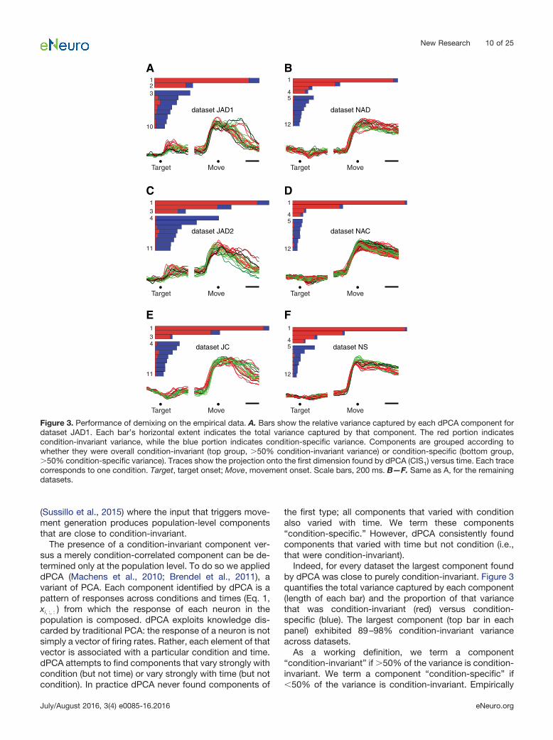
Figure 3. Performance of demixing on the empirical data. A. Bars show the relative variance captured by each dPCA component fordataset JAD1. Each bar’s horizontal extent indicates the total variance captured by that component. The red portion indicatescondition-invariant variance, while the blue portion indicates condition-specific variance. Components are grouped according towhether they were overall condition-invariant (top group, �50% condition-invariant variance) or condition-specific (bottom group,�50% condition-specific variance). Traces show the projection onto the first dimension found by dPCA (CIS1) versus time. Each tracecorresponds to one condition. Target, target onset; Move, movement onset. Scale bars, 200 ms. B—F. Same as A, for the remainingdatasets.

New Research 10 of 25

July/August 2016, 3(4) e0085-16.2016 eNeuro.org

components were either strongly condition-invariant(much greater than 50% condition-invariant variance)or strongly condition-specific (much less than 50%condition-invariant variance). Each bar plot in Figure 3thus groups condition-invariant components at top andcondition-specific components at bottom. All datasetscontained multiple condition-invariant components: re-spectively two, three, three, four, four, and four for data-sets JAD1, JAD2, JC, NAD, NAC, and NS. For a givendataset, we refer to the set of condition-invariant compo-nents as the CIS. We refer to the largest condition-invariant component as CIS1.

Time course of the largest condition-invariantcomponentCIS1, like all the components, is a linear combination ofindividual-neuron responses; it is a “protoneural” re-sponse strongly reflected in single-neuron PSTHs. Thestructure of CIS1 can thus be plotted using the formattypically used for a single-neuron PSTH. Figure 3 does sofor each dataset (colored traces below bar plots).

CIS1 displayed a large and rapid change before move-ment onset that was similar across conditions. This pat-tern was present for all datasets. The sudden changeoccurred �150 ms before movement onset, correspond-ing to 50–100 ms before the first change in EMG activity(not shown). The condition-invariance of the signal can bevisualized by noting that most individual traces (one percondition) overlap. In particular, during the moments be-fore movement onset, CIS1 increases in a similar way andto a similar degree for every condition. Modest differencesbetween conditions appeared primarily around the end ofthe movement and during the subsequent hold period (forreference, movement duration was on average 400 ms).Thus, while CIS1 was not identical across conditions, itwas very close: on average 94% of its structure wasdependent on time but not condition.

The CIS is largeFor every dataset, CIS1 captured the most variance of anysingle component. That is, CIS1 was the component thatmade the largest contribution to the response structure ofindividual neurons. More generally, the set of condition-invariant components (CIS; Fig. 3, top grouping of barswithin each panel) together captured 49–77% of the totalvariance captured by dPCA (respectively 49, 49, 62, 67,77, and 75% for datasets JAD1, JAD2, JC, NAD, NAC,and NS). Thus, not only is a CIS present, it typicallycomprises half or more of the data variance.

While each condition-specific component capturedmuch less variance than CIS1, there were relatively morecondition-specific components (Fig. 3, bottom groupingsof bars) whose combined variance was 23–51% of thetotal variance captured by dPCA. These condition-specific components often contained preparatory activityfollowed by multiphasic responses during the movement.We return later to the structure captured by the condition-specific components.

We did not expect that such a large fraction of thestructure in the data—half or more—would be condition-invariant. Most prior work (including our own) has con-

centrated on the tuned, condition-specific aspects ofneural responses. This is reasonable: the presence of alarge condition-invariant response component is not ob-vious at the single-neuron level. Essentially all neuronshad contributions from condition-specific componentsand were therefore tuned for condition. Such tuning is thetypical focus of analysis in most studies. Yet the fact thatthe CIS is so large argues that its properties should alsobe characterized.

While a few neurons (Fig. 2C,D) had an unusually largecontribution from the condition-invariant components, wefound no evidence for separate populations of condition-invariant and condition-specific neurons. Weights wn,1

were continuously distributed, and could be positive (Fig.2C) or negative (Fig. 2D). We also note that the average�wn, 1� was similar for neurons recorded in PMd and M1,indicating that the CIS is of similar size in the two areas.

Assessing demixingImportantly, dPCA cannot take condition-specific compo-nents and render them into condition-invariant compo-nents. This is true even if condition-specific componentsare strongly condition-correlated (see Materials andMethods for mathematical proof; empirical controls de-scribed below). Thus, the degree to which the populationcontains truly condition-invariant components can be as-sessed by the degree to which dPCA “demixes” respons-es; that is, the degree to which projecting onto orthogonaldimensions yields some response components that areclose to purely condition-invariant. Demixing will be suc-cessful only if such condition-invariant structure is pres-ent in the data.

As noted above, demixing was successful for all data-sets: most components were either strongly condition-invariant or strongly condition-specific. The condition-invariant components (Fig. 3, top grouping of bars in eachpanel) displayed 75–98% condition-invariant variance(mean, 88%). The condition-specific components (bottomgrouping of bars) displayed 74–99% condition-specificvariance (mean, 91%). As discussed above, the largestcomponent—CIS1—was always very close to purelycondition-invariant (mean, 94%). To put these findings incontext, we analyze below a set of model and surrogatepopulations.

A CIS in a network modelIn addition to the six physiological datasets, we analyzedtwo model populations. The models were recurrent neuralnetworks trained (Sussillo and Abbott, 2009; Martens andSutskever, 2011) to generate the empirical patterns ofmuscle activity for two monkeys (Sussillo et al., 2015).Model populations exhibited a CIS (Fig. 4) that closelyresembled that of the neural populations. In particular,there was a sudden change in CIS1 shortly before move-ment onset that was almost purely condition-invariant,with a small amount of condition-specific structure ap-pearing after that transition. Similar to the neural datasets,CIS1 was the largest component of the data and wasoverall very close (99 and 96%) to purely condition-invariant. As with the physiological data, demixing wassuccessful: the model population response could be sep-

New Research 11 of 25

July/August 2016, 3(4) e0085-16.2016 eNeuro.org

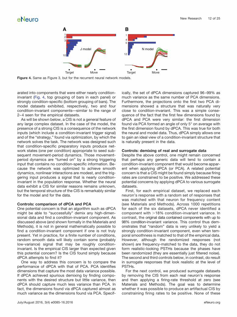
arated into components that were either nearly condition-invariant (Fig. 4, top grouping of bars in each panel) orstrongly condition-specific (bottom grouping of bars). Themodel datasets exhibited, respectively, two and fourcondition-invariant components—similar to the range of2–4 seen for the empirical datasets.

As will be shown below, a CIS is not a general feature ofany large complex dataset. In the case of the model, thepresence of a strong CIS is a consequence of the networkinputs (which include a condition-invariant trigger signal)and of the “strategy,” found via optimization, by which thenetwork solves the task. The network was designed suchthat condition-specific preparatory inputs produce net-work states (one per condition) appropriate to seed sub-sequent movement-period dynamics. Those movement-period dynamics are “turned on” by a strong triggeringinput that contains no condition-specific information. Be-cause the network was optimized to achieve smoothdynamics, nonlinear interactions are modest, and the trig-gering input produces a signal that is nearly condition-invariant in the population response. Whether the neuraldata exhibit a CIS for similar reasons remains unknown,but the temporal structure of the CIS is remarkably similarfor the model and for the data.

Controls: comparison of dPCA and PCAOne potential concern is that an algorithm such as dPCAmight be able to “successfully” demix any high-dimen-sional data and find a condition-invariant component. Asdiscussed above (and shown formally in the Materials andMethods), it is not in general mathematically possible tofind a condition-invariant component if one is not trulypresent. Yet in practice, for a finite number of conditions,random smooth data will likely contain some (probablylow-variance) signal that may be roughly condition-invariant. Is the empirical CIS larger than expected giventhis potential concern? Is the CIS found simply becausedPCA attempts to find it?

One way to address this concern is to compare theperformance of dPCA with that of PCA. PCA identifiesdimensions that capture the most data variance possible.If dPCA achieved spurious demixing by finding compo-nents with the desired structure but little variance, thendPCA should capture much less variance than PCA. Infact, the dimensions found via dPCA captured almost asmuch variance as the dimensions found via PCA. Specif-

ically, the set of dPCA dimensions captured 96–99% asmuch variance as the same number of PCA dimensions.Furthermore, the projections onto the first two PCA di-mensions showed a structure that was naturally veryclose to condition-invariant. This was a simple conse-quence of the fact that the first few dimensions found bydPCA and PCA were very similar: the first dimensionfound via PCA formed an angle of only 5° on average withthe first dimension found by dPCA. This was true for boththe neural and model data. Thus, dPCA simply allows oneto gain an ideal view of a condition-invariant structure thatis naturally present in the data.

Controls: demixing of real and surrogate dataDespite the above control, one might remain concernedthat perhaps any generic data will tend to contain acondition-invariant component that would become appar-ent when applying dPCA (or PCA). A related potentialconcern is that a CIS might be found simply because firingrates are constrained to be positive. We addressed thesepotential concerns by applying dPCA to various surrogatedatasets.

First, for each empirical dataset, we replaced eachneuron’s response with a random set of responses thatwas matched with that neuron for frequency content(see Materials and Methods). Across 1000 repetitionsfor each of the six datasets, dPCA never identified acomponent with �18% condition-invariant variance. Incontrast, the original data contained components with up to98% condition-invariant variance. This control thus dem-onstrates that “random” data is very unlikely to yield astrongly condition-invariant component, even when tem-poral smoothness is matched to that of the empirical data.However, although the randomized responses (notshown) are frequency-matched to the data, they do notform realistic-looking PSTHs because the phases havebeen randomized (they are essentially just filtered noise).The second and third controls below, in contrast, do resultin surrogate responses that look realistic at the level ofPSTHs.

For the next control, we produced surrogate datasetsby removing the CIS from each real neuron’s responseand then applying a firing-rate threshold at zero (seeMaterials and Methods). The goal was to determinewhether it was possible to produce an artifactual CIS byconstraining firing rates to be positive. None of these

A B

J model N model

Target Move Target Move

1 2 3

10

1

4 5

12

Figure 4. Same as Figure 3, but for the recurrent neural network models.

New Research 12 of 25

July/August 2016, 3(4) e0085-16.2016 eNeuro.org

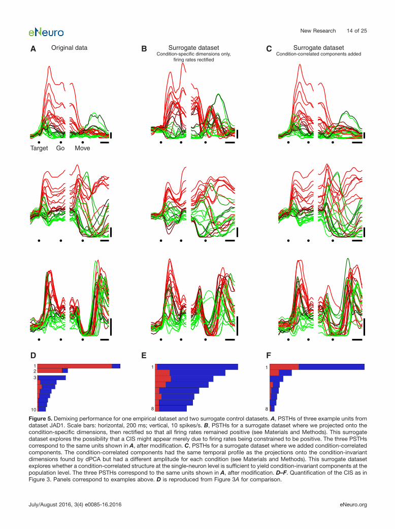
surrogate populations exhibited a CIS. For example, forthe original dataset JAD1, CIS1 contained �90%condition-invariant variance (Fig. 5A,D). The corre-sponding control dataset (Fig. 5B,E) had no CIS com-ponents; all components had �50% condition-invariantvariance. For each of the six surrogate datasets, thefirst component found by dPCA had �21% condition-invariant structure (mean, 6%), in strong contrast to thedata where the first component was always stronglycondition-invariant. Thus, if a population response doesnot contain a CIS, a CIS is not created via the constraintthat firing rates must be positive.

Finally, we wished to perform a control that could ad-dress both of the above concerns while preserving thesurface-level features of the original data as closely aspossible. To do so, we began with the original neuralpopulation (Fig. 5A) and added condition-correlated com-ponents (see Materials and Methods). These condition-correlated components had the same temporal profiles asthe original condition-invariant components, but the re-sponse had a different magnitude for each condition. Thesurrogate population possessed single-neuron responses(Fig. 5C) that looked remarkably similar to the originalresponses, and exhibited changes in the average across-condition firing rate that were almost identical to theoriginal responses. Yet the surrogate population lackedany CIS (Fig. 5F). There were no components with �50%condition-invariant variance for any of the surrogate pop-ulations, even though these are prominent in all the em-pirical datasets.

In summary, the presence of a CIS requires a veryspecific population-level structure and does not arise as asimple consequence of single-neuron response features.Of course, the presence of a CIS is fully consistent withprior work where fits to single-neuron firing rates (e.g.,directional tuning curves) typically require a nondirec-tional component. However, a nondirectional componentwould also be required when fitting the surrogate re-sponses in Figure 5B,C, which contain no CIS. Thus, thepresence of a CIS is consistent with, but not implied by,prior results at the single-neuron level.

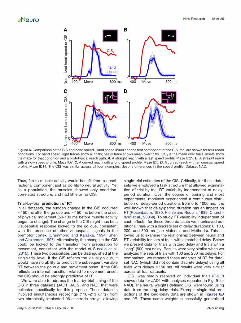
Relationship of the CIS to reach speed and muscleactivityFor the model of Sussillo et al. (2015), the CIS plays an“internal role”: it reflects the arrival of a trigger signal thatrecruits strong dynamics. Might the CIS in the neuralpopulation play a similar internal role? Or might it be morereadily explained in terms of external factors: for example,some aspect of kinematics or muscle activity that is in-variant across conditions? In particular, tuning for reachspeed has been a natural and reasonable way to modelnondirectional aspects of single-neuron responses (Mo-ran and Schwartz, 1999). However, for three reasons, thepopulation-level CIS is unlikely to directly reflect reachspeed. First, the CIS had a rather different profile fromreach speed, which was more sharply phasic (lasting aslittle as �200 ms, depending on the condition) and re-turned to zero as the movement ended (Fig. 6, red traceand blue trace have very different temporal profiles). Sec-

ond, for the task used here, reach speed is not condition-invariant: it varies considerably (�2�) across the differentdistances and reach curvatures. Finally, even the smallvariations present in the CIS across conditions did notparallel variations in reach speed. For monkey J, peakspeed and the peak magnitude of CIS1 were not signifi-cantly correlated (Fig. 6A,B; overall r � 0.097, p � 0.63 forJAD1; r � �0.018, p � 0.93 for JAD2). For monkey N, theywere anticorrelated (r � �0.502, p � 0.008 for NAD, r ��0.364, p � 0.001 for NAC). Thus, the CIS and reachspeed bore little consistent relation. As a side note, thedissimilarity between the CIS and hand speed does notimply that speed information could not be decoded. Usingregression, we could identify a dimension that predictedspeed fairly well (JAD1: r � 0.663; JAD2: r � 0.743; NAD:r � 0.833; NAC: r � 0.720), consistent with prior resultsthat have found strong correlations between neural re-sponses and reach speed (Moran and Schwartz, 1999).The projection onto this dimension, however, capturedmuch less variance (4–16% as much) than CIS1.

A related possibility is that the CIS might reflect nondi-rectional aspects of muscle activity. We performed dPCAon EMG recordings made from 9–11 key arm and shoul-der muscles. The muscle populations did not exhibit astrong CIS. This can be seen by comparing the firstcomponent found via dPCA of the neural data (Fig. 7A,B)with the first component found via dPCA of the muscledata (Fig. 7C,D). The former is nearly condition-invariantwhile the latter is not. For each component found viadPCA, we measured the fraction of variance that wascondition-invariant (the “purity” of condition-invariance)and the variance accounted for relative to the condition-specific components (the “strength” of that component).Unlike the neural populations (Fig. 7E, green) the musclepopulations (purple) did not contain condition-invariantcomponents that were both relatively pure and reasonablystrong; there are no purple symbols in the upper rightcorner. Certainly the muscle population response con-tained some nondirectional aspects: there existed com-ponents in which there was an overall change that wasmostly of the same sign across all conditions, resulting ina proportion of condition-invariant variance as high as0.5–0.75 (purple symbols, left). This variance is not neg-ligible, as evidenced by the fact that it could be furtherreduced via the control manipulations that were applied tothe neural population in Figure 5 (muscle version notshown). However, the components in question capturedrelatively modest amounts of variance, and were notnearly as pure as the components found for the neuralpopulations. Thus, the presence of condition-invariantstructure in the neural population cannot be secondary tofeatures of the muscle activity: only the neural populationcontained components that were both close to purelycondition-invariant and captured a large percentage ofthe overall variance.

The muscle responses further underscore that thepresence or absence of a CIS cannot be inferred fromsurface-level features. Individual muscle responsesclosely resembled neural responses in many ways, andoften showed overall rises in activity across conditions.

New Research 13 of 25

July/August 2016, 3(4) e0085-16.2016 eNeuro.org

1 2 3

10

1

8

D E F

Target Go Move

A B COriginal data Surrogate datasetCondition-specific dimensions only,

firing rates rectified

Surrogate datasetCondition-correlated components added

1

8

Figure 5. Demixing performance for one empirical dataset and two surrogate control datasets. A, PSTHs of three example units fromdataset JAD1. Scale bars: horizontal, 200 ms; vertical, 10 spikes/s. B, PSTHs for a surrogate dataset where we projected onto thecondition-specific dimensions, then rectified so that all firing rates remained positive (see Materials and Methods). This surrogatedataset explores the possibility that a CIS might appear merely due to firing rates being constrained to be positive. The three PSTHscorrespond to the same units shown in A, after modification. C, PSTHs for a surrogate dataset where we added condition-correlatedcomponents. The condition-correlated components had the same temporal profile as the projections onto the condition-invariantdimensions found by dPCA but had a different amplitude for each condition (see Materials and Methods). This surrogate datasetexplores whether a condition-correlated structure at the single-neuron level is sufficient to yield condition-invariant components at thepopulation level. The three PSTHs correspond to the same units shown in A, after modification. D–F. Quantification of the CIS as inFigure 3. Panels correspond to examples above. D is reproduced from Figure 3A for comparison.

New Research 14 of 25

July/August 2016, 3(4) e0085-16.2016 eNeuro.org

Thus, fits to muscle activity would benefit from a nondi-rectional component just as do fits to neural activity. Yetas a population, the muscles showed only condition-correlated structure, and had little or no CIS.

Trial-by-trial prediction of RTIn all datasets, the sudden change in the CIS occurred�150 ms after the go cue and �150 ms before the onsetof physical movement (50-100 ms before muscle activitybegan to change). The change in the CIS might thus be avisuospatial response locked to the go cue, consistentwith the presence of other visuospatial signals in thepremotor cortex (Crammond and Kalaska, 1994; Shenand Alexander, 1997). Alternatively, the change in the CIScould be locked to the transition from preparation tomovement, consistent with the model of Sussillo et al.(2015). These two possibilities can be distinguished at thesingle-trial level. If the CIS reflects the visual go cue, itwould have no ability to predict the subsequent variableRT between the go cue and movement onset. If the CISreflects an internal transition related to movement onset,the CIS should be strongly predictive of RT.

We were able to address the trial-by-trial timing of theCIS in three datasets (JAD1, JAD2, and NAD) that werecollected specifically for this purpose. These datasetsinvolved simultaneous recordings (116–213 units) fromtwo chronically implanted 96-electrode arrays, allowing

single-trial estimates of the CIS. Critically, for these data-sets we employed a task structure that allowed examina-tion of trial-by-trial RT variability independent of delay-period duration. Over the course of training and mostexperiments, monkeys experienced a continuous distri-bution of delay-period durations from 0 to 1000 ms. It iswell known that delay-period duration has an impact onRT (Rosenbaum, 1980; Riehle and Requin, 1989; Church-land et al., 2006a). To study RT variability independent ofsuch effects, for these three datasets we interleaved ad-ditional trials with a discrete set of delay durations: 0, 100,200, and 500 ms (see Materials and Methods). This al-lowed us to examine the relationship between neural andRT variability for sets of trials with a matched delay. Belowwe present data for trials with zero delay and trials with a“long” (500 ms) delay. Results were very similar when weanalyzed the sets of trials with 100 and 200 ms delays. Forcomparison, we repeated these analyses of RT for data-set NAC (which did not contain discrete delays) using alltrials with delays �150 ms. All results were very similaracross all four datasets.

CIS1 was readily resolved on individual trials (Fig. 8shows data for JAD1 with analyses repeated in Fig. 9 forNAD). The neural weights defining CIS1 were found usingdata from the long-delay trials. Example single-trial pro-jections of the long-delay data are shown in Figures 8Band 9B. These same weights successfully generalized

A B

C D

handspeed

CIS1

−400 Move 800 ms0

1

Nor

mal

ized

han

d sp

eed

or C

IS1

−400 Move 800 ms0

1

Nor

mal

ized

han

d sp

eed

or C

IS1

−400 Move 800 ms

0

1

−400 Move 800 ms

0

1

Figure 6. Comparison of the CIS and hand speed. Hand speed (blue) and the first component of the CIS (red) are shown for four reachconditions. For hand speed, light traces show all trials; heavy trace shows mean over trials. CIS1 is the mean over trials. Insets showthe maze for that condition and a prototypical reach path. A, A straight reach with a fast speed profile. Maze ID25. B, A straight reachwith a slow speed profile. Maze ID7. C, A curved reach with a long speed profile. Maze ID5. D, A curved reach with an unusual speedprofile. Maze ID14. The CIS was similar across all four examples, despite differences in the speed profile. Dataset NAD.

New Research 15 of 25

July/August 2016, 3(4) e0085-16.2016 eNeuro.org

and revealed an essentially identical CIS1 for the zero-delay trials (Figs. 8A, 9A). The latency of the rise time ofCIS1, relative to the go cue, varied from trial to trial. Toestimate this latency, we measured when CIS1 crossed acriterion value following the go cue (Figs. 8A,B, 9A,B, grayline). We selected a 50% criterion that is simply a practicaland robust criterion for estimating rise time (and shouldnot be interpreted as suggesting a physiological thresh-

old). The estimated rise time strongly predicted the sub-sequent RT on individual trials (Figs. 8C, 9C) for bothlong-delay (blue) and zero-delay (red) trials. This was trueacross all analyzed datasets: the average correlation wasr � 0.805 for long-delay trials, and r � 0.827 for zero-delay trials.

The CIS strongly predicts RT on a single-trial basis, butdoes it do so more accurately than other reasonable

E

neural activity

DC

BA

Neural dataJAD1

Neural dataNAD

Muscle data, J Muscle data, N

0.25 0.5 1 10 var. in kth C.I. dim. / var. in kth cond.-spec. dim.

0.5

0.75

1

Fra

c. v

ar. i

n C

.I. d

im. t

hat i

s C

.I.

muscle activity

1 2 3

10

1

4 5

12

135

124

Figure 7. Comparison of dPCA applied to neural and muscle populations. A, B, Demixing performance (bars) and the projection ontothe first dimension found by dPCA (CIS1) for neural datasets JAD1 and NAD. Each trace corresponds to one condition. These panelsare reproduced from Figure 3A,B for comparison with the corresponding analysis of EMG. Dots indicate target onset and movementonset. Scale bar, 200 ms. C, D, Similar analysis as in A and B, but for the muscle populations recorded for monkeys J and N. Muscleactivity was recorded for the same sets of conditions as for the neural data in A and B. E, To compare the prevalence of acondition-invariant structure in the neural and muscle populations, we focused on nominally “condition-invariant” components with�50% condition-invariant variance. There were many such components for the neural populations (green) and 1–2 such componentsfor each of the muscle populations (purple). For each such component, two measurements were taken: the fraction of thecomponent’s variance that was condition-invariant (vertical axis) and the total variance captured. The latter was expressed innormalized terms: the variance captured by the kth nominally “condition-invariant” component divided by the total variance capturedby the kth “condition-specific” component (horizontal axis). Only the neural datasets contained components that were both stronglycondition-invariant (high on the vertical axis) and that captured relatively large amounts of variance (to the right on the horizontal axis).Heaviest symbols correspond to the first dimension found by dPCA for each dataset; higher-numbered dimensions are plotted asprogressively lighter symbols. Dashed gray line highlights variance ratio of unity. Circles, monkey J datasets; squares, monkey Ndatasets.

New Research 16 of 25

July/August 2016, 3(4) e0085-16.2016 eNeuro.org

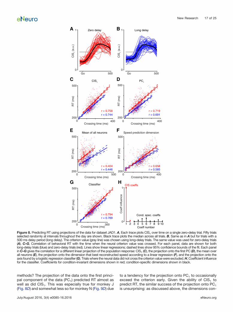
methods? The projection of the data onto the first princi-pal component of the data (PC1) predicted RT almost aswell as did CIS1. This was especially true for monkey J(Fig. 8D) and somewhat less so for monkey N (Fig. 9D) due

to a tendency for the projection onto PC1 to occasionallyexceed the criterion early. Given the ability of CIS1 topredict RT, the similar success of the projection onto PC1

is unsurprising: as discussed above, the dimensions con-

Classifier

CIS1 PC1

Mean of all neurons

A

G

C

E F

H

D

Speed prediction dimension

B

r = 0.744

0 400Crossing time (ms)

200

500

RT

(m

s)

r = 0.758r = 0.691

0 400Crossing time (ms)

200

500

RT

(m

s)

r = 0.719

r = 0.446

0 500Crossing time (ms)

200

500

RT

(m

s)

r = 0.404r = 0.585

0 400Crossing time (ms)

200

500

RT

(m

s)

r = 0.658

r = 0.769

0 300Crossing time (ms)

200

500

RT

(m

s)

r = 0.794

CIS coeffs

Cond. spec. coeffs

1 2 5 6 8 93 4 7 10Coeff number

0

1

Coe

ff in

fluen

ce

Go 5000

1

CIS

1 (a

.u.)

Go 5000

1

CIS

1 (a

.u.)

Zero delay Long delay

Figure 8. Predicting RT using projections of the data for dataset JAD1. A, Each trace plots CIS1 over time on a single zero-delay trial. Fifty trialsselected randomly at intervals throughout the day are shown. Black trace plots the median across all trials. B, Same as in A but for trials with a500 ms delay period (long delay). The criterion value (gray line) was chosen using long-delay trials. The same value was used for zero-delay trials(A). C–G, Correlation of behavioral RT with the time when the neural criterion value was crossed. For each panel, data are shown for bothlong-delay trials (blue) and zero-delay trials (red). Lines show linear regressions; dashed lines show 95% confidence bounds of the fit. Each panelin C–G gives the correlation for a different linear projection of the population response: CIS1 (C), the projection onto the first PC (D), the mean overall neurons (E), the projection onto the dimension that best reconstructed speed according to a linear regression (F), and the projection onto theaxis found by a logistic regression classifier (G). Trials where the neural data did not cross the criterion value were excluded. H, Coefficient influencefor the classifier. Coefficients for condition-invariant dimensions shown in red; condition-specific dimensions shown in black.

New Research 17 of 25

July/August 2016, 3(4) e0085-16.2016 eNeuro.org

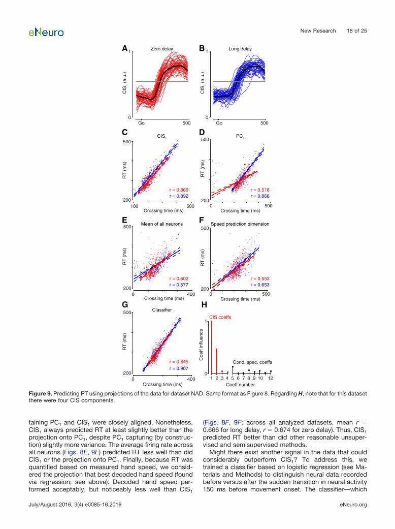
taining PC1 and CIS1 were closely aligned. Nonetheless,CIS1 always predicted RT at least slightly better than theprojection onto PC1, despite PC1 capturing (by construc-tion) slightly more variance. The average firing rate acrossall neurons (Figs. 8E, 9E) predicted RT less well than didCIS1 or the projection onto PC1. Finally, because RT wasquantified based on measured hand speed, we consid-ered the projection that best decoded hand speed (foundvia regression; see above). Decoded hand speed per-formed acceptably, but noticeably less well than CIS1

(Figs. 8F, 9F; across all analyzed datasets, mean r �0.666 for long delay, r � 0.674 for zero delay). Thus, CIS1

predicted RT better than did other reasonable unsuper-vised and semisupervised methods.

Might there exist another signal in the data that couldconsiderably outperform CIS1? To address this, wetrained a classifier based on logistic regression (see Ma-terials and Methods) to distinguish neural data recordedbefore versus after the sudden transition in neural activity150 ms before movement onset. The classifier—which

Classifier

CIS1 PC1

Mean of all neurons

A

C

G

E F

H

D

Speed prediction dimension

B

CIS coeffs

Cond. spec. coeffs

1 2 3 6 7 94 5 8 10 12Coeff number

0

1

Coe

ff in

fluen

ce

r = 0.653

0 500Crossing time (ms)

200

500

RT

(m

s)

r = 0.553r = 0.577

0 400Crossing time (ms)

200

500

RT

(m

s)

r = 0.602

r = 0.907

0 400Crossing time (ms)

200

500

RT

(m

s)

r = 0.845

r = 0.892

100 500Crossing time (ms)

200

500

RT

(m

s)

r = 0.869r = 0.866

0 500Crossing time (ms)

200

500

RT

(m

s)

r = 0.518

Go 5000

1

CIS

1 (a

.u.)

Go 5000

1

CIS

1 (a

.u.)

Zero delay Long delay

Figure 9. Predicting RT using projections of the data for dataset NAD. Same format as Figure 8. Regarding H, note that for this datasetthere were four CIS components.

New Research 18 of 25

July/August 2016, 3(4) e0085-16.2016 eNeuro.org

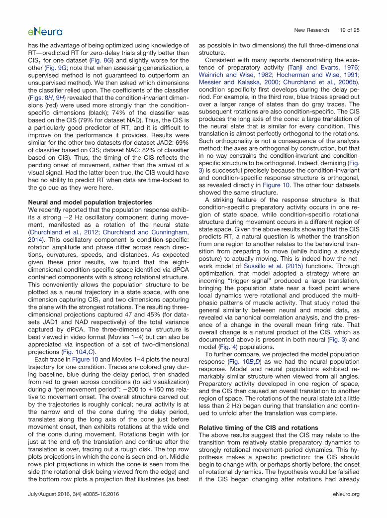
has the advantage of being optimized using knowledge ofRT—predicted RT for zero-delay trials slightly better thanCIS1 for one dataset (Fig. 8G) and slightly worse for theother (Fig. 9G; note that when assessing generalization, asupervised method is not guaranteed to outperform anunsupervised method). We then asked which dimensionsthe classifier relied upon. The coefficients of the classifier(Figs. 8H, 9H) revealed that the condition-invariant dimen-sions (red) were used more strongly than the condition-specific dimensions (black); 74% of the classifier wasbased on the CIS (79% for dataset NAD). Thus, the CIS isa particularly good predictor of RT, and it is difficult toimprove on the performance it provides. Results weresimilar for the other two datasets (for dataset JAD2: 69%of classifier based on CIS; dataset NAC: 82% of classifierbased on CIS). Thus, the timing of the CIS reflects thepending onset of movement, rather than the arrival of avisual signal. Had the latter been true, the CIS would havehad no ability to predict RT when data are time-locked tothe go cue as they were here.

Neural and model population trajectoriesWe recently reported that the population response exhib-its a strong �2 Hz oscillatory component during move-ment, manifested as a rotation of the neural state(Churchland et al., 2012; Churchland and Cunningham,2014). This oscillatory component is condition-specific:rotation amplitude and phase differ across reach direc-tions, curvatures, speeds, and distances. As expectedgiven these prior results, we found that the eight-dimensional condition-specific space identified via dPCAcontained components with a strong rotational structure.This conveniently allows the population structure to beplotted as a neural trajectory in a state space, with onedimension capturing CIS1 and two dimensions capturingthe plane with the strongest rotations. The resulting three-dimensional projections captured 47 and 45% (for data-sets JAD1 and NAD respectively) of the total variancecaptured by dPCA. The three-dimensional structure isbest viewed in video format (Movies 1–4) but can also beappreciated via inspection of a set of two-dimensionalprojections (Fig. 10A,C).

Each trace in Figure 10 and Movies 1–4 plots the neuraltrajectory for one condition. Traces are colored gray dur-ing baseline, blue during the delay period, then shadedfrom red to green across conditions (to aid visualization)during a “perimovement period”: �200 to �150 ms rela-tive to movement onset. The overall structure carved outby the trajectories is roughly conical; neural activity is atthe narrow end of the cone during the delay period,translates along the long axis of the cone just beforemovement onset, then exhibits rotations at the wide endof the cone during movement. Rotations begin with (orjust at the end of) the translation and continue after thetranslation is over, tracing out a rough disk. The top rowplots projections in which the cone is seen end-on. Middlerows plot projections in which the cone is seen from theside (the rotational disk being viewed from the edge) andthe bottom row plots a projection that illustrates (as best

as possible in two dimensions) the full three-dimensionalstructure.

Consistent with many reports demonstrating the exis-tence of preparatory activity (Tanji and Evarts, 1976;Weinrich and Wise, 1982; Hocherman and Wise, 1991;Messier and Kalaska, 2000; Churchland et al., 2006b),condition specificity first develops during the delay pe-riod. For example, in the third row, blue traces spread outover a larger range of states than do gray traces. Thesubsequent rotations are also condition-specific. The CISproduces the long axis of the cone: a large translation ofthe neural state that is similar for every condition. Thistranslation is almost perfectly orthogonal to the rotations.Such orthogonality is not a consequence of the analysismethod: the axes are orthogonal by construction, but thatin no way constrains the condition-invariant and condition-specific structure to be orthogonal. Indeed, demixing (Fig.3) is successful precisely because the condition-invariantand condition-specific response structure is orthogonal,as revealed directly in Figure 10. The other four datasetsshowed the same structure.

A striking feature of the response structure is thatcondition-specific preparatory activity occurs in one re-gion of state space, while condition-specific rotationalstructure during movement occurs in a different region ofstate space. Given the above results showing that the CISpredicts RT, a natural question is whether the transitionfrom one region to another relates to the behavioral tran-sition from preparing to move (while holding a steadyposture) to actually moving. This is indeed how the net-work model of Sussillo et al. (2015) functions. Throughoptimization, that model adopted a strategy where anincoming “trigger signal” produced a large translation,bringing the population state near a fixed point wherelocal dynamics were rotational and produced the multi-phasic patterns of muscle activity. That study noted thegeneral similarity between neural and model data, asrevealed via canonical correlation analysis, and the pres-ence of a change in the overall mean firing rate. Thatoverall change is a natural product of the CIS, which asdocumented above is present in both neural (Fig. 3) andmodel (Fig. 4) populations.

To further compare, we projected the model populationresponse (Fig. 10B,D) as we had the neural populationresponse. Model and neural populations exhibited re-markably similar structure when viewed from all angles.Preparatory activity developed in one region of space,and the CIS then caused an overall translation to anotherregion of space. The rotations of the neural state (at a littleless than 2 Hz) began during that translation and contin-ued to unfold after the translation was complete.

Relative timing of the CIS and rotationsThe above results suggest that the CIS may relate to thetransition from relatively stable preparatory dynamics tostrongly rotational movement-period dynamics. This hy-pothesis makes a specific prediction: the CIS shouldbegin to change with, or perhaps shortly before, the onsetof rotational dynamics. The hypothesis would be falsifiedif the CIS began changing after rotations had already

New Research 19 of 25

July/August 2016, 3(4) e0085-16.2016 eNeuro.org

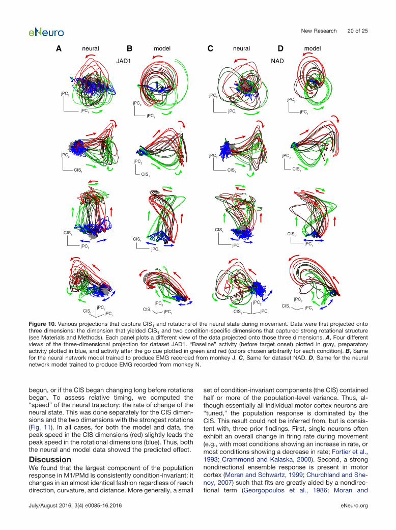
begun, or if the CIS began changing long before rotationsbegan. To assess relative timing, we computed the“speed” of the neural trajectory: the rate of change of theneural state. This was done separately for the CIS dimen-sions and the two dimensions with the strongest rotations(Fig. 11). In all cases, for both the model and data, thepeak speed in the CIS dimensions (red) slightly leads thepeak speed in the rotational dimensions (blue). Thus, boththe neural and model data showed the predicted effect.

DiscussionWe found that the largest component of the populationresponse in M1/PMd is consistently condition-invariant: itchanges in an almost identical fashion regardless of reachdirection, curvature, and distance. More generally, a small

set of condition-invariant components (the CIS) containedhalf or more of the population-level variance. Thus, al-though essentially all individual motor cortex neurons are“tuned,” the population response is dominated by theCIS. This result could not be inferred from, but is consis-tent with, three prior findings. First, single neurons oftenexhibit an overall change in firing rate during movement(e.g., with most conditions showing an increase in rate, ormost conditions showing a decrease in rate; Fortier et al.,1993; Crammond and Kalaska, 2000). Second, a strongnondirectional ensemble response is present in motorcortex (Moran and Schwartz, 1999; Churchland and She-noy, 2007) such that fits are greatly aided by a nondirec-tional term (Georgopoulos et al., 1986; Moran and

jPC1

jPC2

CIS1 jPC1

jPC2

jPC1

jPC2

C DBA

CIS1jPC1

jPC2

CIS1

jPC1

CIS1

jPC2

CIS1

jPC1

CIS1

jPC2

jPC1

jPC2

CIS1

jPC2

CIS1 jPC1

jPC2

CIS1

jPC1

CIS1

jPC1

CIS1

jPC2

CIS1 jPC1

jPC2

jPC1

jPC2

JAD1

neural model

NAD

neural model

Figure 10. Various projections that capture CIS1 and rotations of the neural state during movement. Data were first projected ontothree dimensions: the dimension that yielded CIS1 and two condition-specific dimensions that captured strong rotational structure(see Materials and Methods). Each panel plots a different view of the data projected onto those three dimensions. A, Four differentviews of the three-dimensional projection for dataset JAD1. “Baseline” activity (before target onset) plotted in gray, preparatoryactivity plotted in blue, and activity after the go cue plotted in green and red (colors chosen arbitrarily for each condition). B, Samefor the neural network model trained to produce EMG recorded from monkey J. C, Same for dataset NAD. D, Same for the neuralnetwork model trained to produce EMG recorded from monkey N.

New Research 20 of 25

July/August 2016, 3(4) e0085-16.2016 eNeuro.org

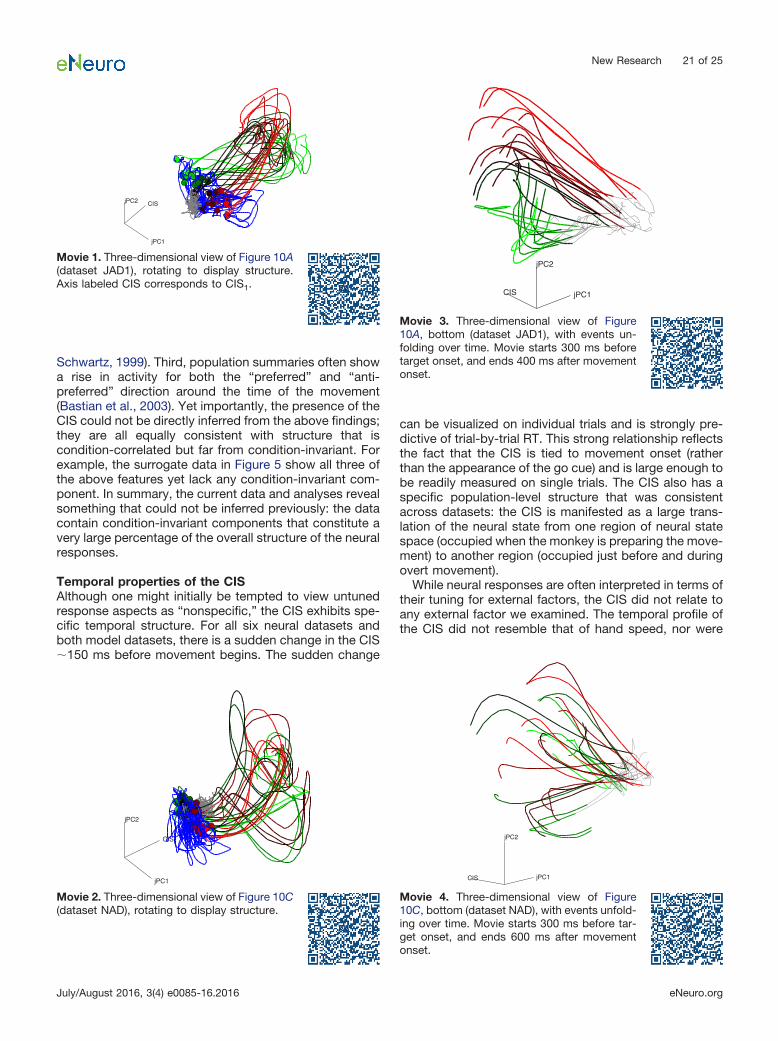
Schwartz, 1999). Third, population summaries often showa rise in activity for both the “preferred” and “anti-preferred” direction around the time of the movement(Bastian et al., 2003). Yet importantly, the presence of theCIS could not be directly inferred from the above findings;they are all equally consistent with structure that iscondition-correlated but far from condition-invariant. Forexample, the surrogate data in Figure 5 show all three ofthe above features yet lack any condition-invariant com-ponent. In summary, the current data and analyses revealsomething that could not be inferred previously: the datacontain condition-invariant components that constitute avery large percentage of the overall structure of the neuralresponses.

Temporal properties of the CISAlthough one might initially be tempted to view untunedresponse aspects as “nonspecific,” the CIS exhibits spe-cific temporal structure. For all six neural datasets andboth model datasets, there is a sudden change in the CIS�150 ms before movement begins. The sudden change

can be visualized on individual trials and is strongly pre-dictive of trial-by-trial RT. This strong relationship reflectsthe fact that the CIS is tied to movement onset (ratherthan the appearance of the go cue) and is large enough tobe readily measured on single trials. The CIS also has aspecific population-level structure that was consistentacross datasets: the CIS is manifested as a large trans-lation of the neural state from one region of neural statespace (occupied when the monkey is preparing the move-ment) to another region (occupied just before and duringovert movement).

While neural responses are often interpreted in terms oftheir tuning for external factors, the CIS did not relate toany external factor we examined. The temporal profile ofthe CIS did not resemble that of hand speed, nor were

CIS

jPC1

jPC2

Movie 1. Three-dimensional view of Figure 10A(dataset JAD1), rotating to display structure.Axis labeled CIS corresponds to CIS1.

CIS

jPC1

jPC2

Movie 2. Three-dimensional view of Figure 10C(dataset NAD), rotating to display structure.

jPC1

jPC2

CIS

Movie 3. Three-dimensional view of Figure10A, bottom (dataset JAD1), with events un-folding over time. Movie starts 300 ms beforetarget onset, and ends 400 ms after movementonset.

jPC1

jPC2

CIS

Movie 4. Three-dimensional view of Figure10C, bottom (dataset NAD), with events unfold-ing over time. Movie starts 300 ms before tar-get onset, and ends 600 ms after movementonset.

New Research 21 of 25

July/August 2016, 3(4) e0085-16.2016 eNeuro.org

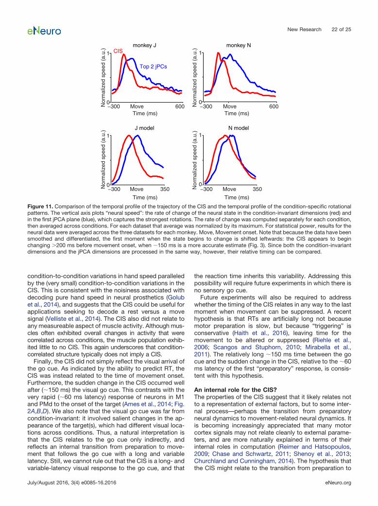
condition-to-condition variations in hand speed paralleledby the (very small) condition-to-condition variations in theCIS. This is consistent with the noisiness associated withdecoding pure hand speed in neural prosthetics (Golubet al., 2014), and suggests that the CIS could be useful forapplications seeking to decode a rest versus a movesignal (Velliste et al., 2014). The CIS also did not relate toany measureable aspect of muscle activity. Although mus-cles often exhibited overall changes in activity that werecorrelated across conditions, the muscle population exhib-ited little to no CIS. This again underscores that condition-correlated structure typically does not imply a CIS.

Finally, the CIS did not simply reflect the visual arrival ofthe go cue. As indicated by the ability to predict RT, theCIS was instead related to the time of movement onset.Furthermore, the sudden change in the CIS occurred wellafter (�150 ms) the visual go cue. This contrasts with thevery rapid (�60 ms latency) response of neurons in M1and PMd to the onset of the target (Ames et al., 2014; Fig.2A,B,D). We also note that the visual go cue was far fromcondition-invariant: it involved salient changes in the ap-pearance of the target(s), which had different visual loca-tions across conditions. Thus, a natural interpretation isthat the CIS relates to the go cue only indirectly, andreflects an internal transition from preparation to move-ment that follows the go cue with a long and variablelatency. Still, we cannot rule out that the CIS is a long- andvariable-latency visual response to the go cue, and that

the reaction time inherits this variability. Addressing thispossibility will require future experiments in which there isno sensory go cue.

Future experiments will also be required to addresswhether the timing of the CIS relates in any way to the lastmoment when movement can be suppressed. A recenthypothesis is that RTs are artificially long not becausemotor preparation is slow, but because “triggering” isconservative (Haith et al., 2016), leaving time for themovement to be altered or suppressed (Riehle et al.,2006; Scangos and Stuphorn, 2010; Mirabella et al.,2011). The relatively long �150 ms time between the gocue and the sudden change in the CIS, relative to the �60ms latency of the first “preparatory” response, is consis-tent with this hypothesis.

An internal role for the CIS?The properties of the CIS suggest that it likely relates notto a representation of external factors, but to some inter-nal process—perhaps the transition from preparatoryneural dynamics to movement-related neural dynamics. Itis becoming increasingly appreciated that many motorcortex signals may not relate cleanly to external parame-ters, and are more naturally explained in terms of theirinternal roles in computation (Reimer and Hatsopoulos,2009; Chase and Schwartz, 2011; Shenoy et al., 2013;Churchland and Cunningham, 2014). The hypothesis thatthe CIS might relate to the transition from preparation to

J model N model

monkey J monkey N

−300 Move 350

Time (ms)

0

1

Nor

mal

ized

spe

ed (

a.u.

)−300 Move 350

Time (ms)

0

1

Nor

mal

ized

spe

ed (

a.u.

)−300 Move 600

Time (ms)

0

1

Nor

mal

ized

spe

ed (

a.u.

)−300 Move 600

Time (ms)

0

1

Nor

mal

ized

spe

ed (

a.u.

)CIS

Top 2 jPCs

Figure 11. Comparison of the temporal profile of the trajectory of the CIS and the temporal profile of the condition-specific rotationalpatterns. The vertical axis plots “neural speed”: the rate of change of the neural state in the condition-invariant dimensions (red) andin the first jPCA plane (blue), which captures the strongest rotations. The rate of change was computed separately for each condition,then averaged across conditions. For each dataset that average was normalized by its maximum. For statistical power, results for theneural data were averaged across the three datasets for each monkey. Move, Movement onset. Note that because the data have beensmoothed and differentiated, the first moment when the state begins to change is shifted leftwards: the CIS appears to beginchanging �200 ms before movement onset, when �150 ms is a more accurate estimate (Fig. 3). Since both the condition-invariantdimensions and the jPCA dimensions are processed in the same way, however, their relative timing can be compared.

New Research 22 of 25

July/August 2016, 3(4) e0085-16.2016 eNeuro.org

movement is further suggested by the finding that thenetwork model of Sussillo et al. (2015) exhibits a verysimilar CIS—and similar overall population structure—tothe neural data (Figs. 4, 10). In the case of the model, theCIS is a consequence of the externally delivered triggersignal, and is in turn the cause of the change in neuraldynamics that generates movement. The original analysesin Sussillo et al. did not focus on or attempt to isolate aCIS. Yet a condition-invariant translation is clearly presentin one key analysis (Sussillo et al., 2015, their Fig. 6) andcan be seen to bring the set of network states close to afixed point with rotational dynamics. Whether this inter-pretation is also correct for the data is of course stilluncertain, but the population response structure is re-markably similar for the model and data. This interpreta-tion is also supported by both the overall timing of the CIS(it occurs just as, or even slightly before, the onset ofrotational dynamics; Fig. 11) and the remarkably strongcorrelation between the change in the CIS and the mo-ment when movement begins (Figs. 8, 9).

Other, not necessarily exclusive explanations are alsolikely. For example, the CIS could activate, suppress, oralter how the local circuit processes feedback (Cluff et al.,2015). Similarly, the CIS could relate to an overall modu-lation of downstream reflexes or to a disengagement ofpostural control (Kurtzer et al., 2005; Cluff and Scott,2016). After all, the initiation of activity that drives move-ment must presumably be accompanied by cessation ofthe activity that held the hand in place during the delayperiod. This is true even of the model of Sussillo et al., whichis involved in a rudimentary form of postural control duringthe delay period: producing a constant pattern of muscleactivity. For that model, the CIS produces the transitionaway from the stable dynamics that maintain constant out-puts, and towards oscillatory dynamics that produce themovement-driving patterns of muscle activity.

What inputs might produce a CIS?If motor cortex undergoes a large condition-invariantchange prior to movement, what drives that change?What other area(s) might supply the relevant input? Anumber of candidate regions exist, including the basalganglia (Romo et al., 1992; Hauber, 1998), superior col-liculus (Werner, 1993; Philipp and Hoffmann, 2014), pari-etal cortex (Scherberger and Andersen, 2007; Pesaranet al., 2008), supplementary motor area (Orgogozo andLarsen, 1979; Eccles, 1982; Romo and Schultz, 1992), thedentate nucleus of the cerebellum (Meyer-Lohmann et al.,1977), and, in rodents, secondary motor cortex (Murakamiet al., 2014). Moreover, the origin of the CIS may dependon the task: movements elicited by a strong sensory cuemay be generated differently from self-initiated move-ments (Kurata and Wise, 1988) or movements that mustbe made very rapidly (Perfiliev et al., 2010). Along similarlines, RTs can be remarkably short when the go cue isprovided by a mechanical perturbation of the limb (Evartsand Tanji, 1976; Pruszynski et al., 2008). These short RTsmay be related to the finding that some neurons show arapid perturbation-driven response that is invariant acrossperturbation directions (Herter et al., 2009, their Fig. 3C).

It is thus vital that future studies address whether a similarCIS is present in motor cortex across the many possiblesensory cues and internal events that can be responsiblefor causing movement initiation.

SummaryIn summary, our results build upon the long-standing obser-vation that responses are often correlated across conditionsat the single-neuron level. Our results reveal that this generalsurface-level structure reflects a very particular kind of un-derlying structure: a large condition-invariant response com-ponent with timing closely tied to movement onset. Thisadds to a small but growing list of “untuned” responseaspects that might initially appear incidental, but may in factplay important computational roles.

ReferencesAmes KC, Ryu SI, Shenoy KV (2014) Neural dynamics of reaching

following incorrect or absent motor preparation. Neuron 81:438–451. CrossRef Medline

Bastian A, Schöner G, Riehle A (2003) Preshaping and continuousevolution of motor cortical representations during movement prep-aration. Eur J Neurosci 18:2047–2058. Medline

Brendel W, Romo R, Machens C (2011) Demixed principal compo-nent analysis. Adv Neural Info Process Syst 24:1–9.

Chase SM, Schwartz AB (2011) Inference from populations: goingbeyond models. Prog Brain Res 192:103–112. CrossRef Medline

Churchland AK, Kiani R, Shadlen MN (2008) Decision-making withmultiple alternatives. Nat Neurosci 11:693–702. CrossRef Medline

Churchland MM, Shenoy KV (2007) Temporal complexity and heter-ogeneity of single-neuron activity in premotor and motor cortex. JNeurophysiol 97:4235–4257. CrossRef Medline

Churchland MM, Cunningham JP (2014) A dynamical basis set forgenerating reaches. Cold Spring Harb Symp Quant Biol 79:67–80.CrossRef Medline

Churchland MM, Yu BM, Ryu SI, Santhanam G, Shenoy KV (2006a)Neural variability in premotor cortex provides a signature of motorpreparation. J Neurosci 26:3697–3712. CrossRef Medline

Churchland MM, Santhanam G, Shenoy KV (2006b) Preparatoryactivity in premotor and motor cortex reflects the speed of theupcoming reach. J Neurophysiol 96:3130–3146. CrossRef Med-line

Churchland MM, Cunningham JP, Kaufman MT, Ryu SI, Shenoy KV(2010) Cortical preparatory activity: representation of movement orfirst cog in a dynamical machine? Neuron 68:387–400. CrossRefMedline

Churchland MM, Cunningham JP, Kaufman MT, Foster JD, Nuyu-jukian P, Ryu SI, Shenoy KV (2012) Neural population dynamicsduring reaching. Nature 487:51–56. CrossRef Medline

Cluff T, Scott SH (2016) Online corrections are faster because move-ment initiation must disengage postural control. Motor Control20:162–170. CrossRef Medline

Cluff T, Crevecoeur F, Scott SH (2015) A perspective on multisensoryintegration and rapid perturbation responses. Vision Res 110:215–222. CrossRef Medline

Confais J, Kilavik BE, Ponce-Alvarez A, Riehle A (2012) On theanticipatory precue activity in motor cortex. J Neurosci 32:15359–15368. CrossRef Medline

Crammond DJ, Kalaska JF (1994) Modulation of preparatory neuro-nal activity in dorsal premotor cortex due to stimulus-responsecompatibility. J Neurophysiol 71:1281–1284. Medline

Crammond DJ, Kalaska JF (2000) Prior information in motor andpremotor cortex: activity during the delay period and effect onpre-movement activity. J Neurophysiol 84:986–1005. Medline

Eccles JC (1982) The initiation of voluntary movements by the sup-plementary motor area. Arch Psychiatr Nervenkr 231:423–441.Medline

New Research 23 of 25

July/August 2016, 3(4) e0085-16.2016 eNeuro.org

Erlhagen W, Schöner G (2002) Dynamic field theory of movementpreparation. Psychol Rev 109:545–572. Medline

Evarts EV (1968) Relation of pyramidal tract activity to force exertedduring voluntary movement. J Neurophysiol 31:14–27. Medline

Evarts EV, Tanji J (1976) Reflex and intended responses in motorcortex pyramidal tract neurons of monkey. J Neurophysiol 39:1069–1080. Medline

Fortier PA, Smith AM, Kalaska JF (1993) Comparison of cerebellarand motor cortex activity during reaching: directional tuning andresponse variability. J Neurophysiol 69:1136–1149. Medline

Georgopoulos AP, Schwartz AB, Kettner RE (1986) Neuronal popu-lation coding of movement direction. Science 233:1416–1419.Medline

Godschalk M, Lemon RN, Kuypers HG, van der Steen J (1985) Theinvolvement of monkey premotor cortex neurones in preparationof visually cued arm movements. Behav Brain Res 18:143–157.Medline

Golub MD, Yu BM, Schwartz AB, Chase SM (2014) Motor corticalcontrol of movement speed with implications for brain-machineinterface control. J Neurophysiol 112:411–429. CrossRef Medline

Haith AM, Pakpoor J, Krakauer JW (2016) Independence of move-ment preparation and movement initiation. J Neurosci 36:3007–3015. CrossRef Medline

Hanks TD, Mazurek ME, Kiani R, Hopp E, Shadlen MN (2011)Elapsed decision time affects the weighting of prior probability ina perceptual decision task. J Neurosci 31:6339–6352. CrossRefMedline

Hauber W (1998) Involvement of basal ganglia transmitter systems inmovement initiation. Prog Neurobiol 56:507–540. Medline

Hennequin G, Vogels TP, Gerstner W (2014) Optimal control oftransient dynamics in balanced networks supports generation ofcomplex movements. Neuron 82:1394–1406. CrossRef Medline

Herter TM, Korbel T, Scott SH (2009) Comparison of neural re-sponses in primary motor cortex to transient and continuous loadsduring posture. J Neurophysiol 101:150–163. CrossRef Medline

Hocherman S, Wise SP (1991) Effects of hand movement path onmotor cortical activity in awake, behaving rhesus monkeys. ExpBrain Res 83:285–302. Medline

Johnson MT, Coltz JD, Hagen MC, Ebner TJ (1999) Visuomotorprocessing as reflected in the directional discharge of premotorand primary motor cortex neurons. J Neurophysiol 81:875–894.Medline

Kaufman MT, Churchland MM, Santhanam G, Yu BM, Afshar A, RyuSI, Shenoy KV (2010) Roles of monkey premotor neuron classes inmovement preparation and execution. J Neurophysiol 104:799–810. CrossRef Medline

Kaufman MT, Churchland MM, Shenoy KV (2013) The roles of mon-key M1 neuron classes in movement preparation and execution. JNeurophysiol 110:817–825. CrossRef Medline

Kobak D, Brendel W, Constantinidis C, Feierstein CE, Kepecs A,Mainen ZF, Qi XL, Romo R, Uchida N, Machens CK (2016) De-mixed principal component analysis of neural population data.eLife 5. CrossRef Medline

Kurata K (1989) Distribution of neurons with set- and movement-related activity before hand and foot movements in the premotorcortex of rhesus monkeys. Exp Brain Res 77:245–256. Medline

Kurata K, Wise SP (1988) Premotor and supplementary motor cortexin rhesus monkeys: neuronal activity during externally- andinternally-instructed motor tasks. Exp Brain Res 72:237–248. Med-line

Kurtzer I, Herter TM, Scott SH (2005) Random change in cortical loadrepresentation suggests distinct control of posture and movement.Nat Neurosci 8:498–504. CrossRef Medline

Machens CK, Romo R, Brody CD (2010) Functional, but not anatom-ical, separation of “what” and “when” in prefrontal cortex. J Neu-rosci 30:350–360. CrossRef Medline

Martens J, Sutskever I (2011) Learning recurrent neural networkswith hessian-free optimization. Paper presented at 28th Interna-tional Conference on Machine Learning (ICML-11), Bellevue, WA,June.

Messier J, Kalaska JF (2000) Covariation of primate dorsal premotorcell activity with direction and amplitude during a memorized-delay reaching task. J Neurophysiol 84:152–165. Medline

Meyer-Lohmann J, Hore J, Brooks VB (1977) Cerebellar participationin generation of prompt arm movements. J Neurophysiol 40:1038–1050. Medline

Mirabella G, Pani P, Ferraina S (2011) Neural correlates of cognitivecontrol of reaching movements in the dorsal premotor cortex ofrhesus monkeys. J Neurophysiol 106:1454–1466. CrossRef Med-line

Moran DW, Schwartz AB (1999) Motor cortical representation ofspeed and direction during reaching. J Neurophysiol 82:2676–2692. Medline

Murakami M, Mainen ZF (2015) Preparing and selecting actions withneural populations: toward cortical circuit mechanisms. Curr OpinNeurobiol 33:40–46. CrossRef Medline

Murakami M, Vicente MI, Costa GM, Mainen ZF (2014) Neural ante-cedents of self-initiated actions in secondary motor cortex. NatNeurosci 17:1574–1582. CrossRef Medline

Orgogozo JM, Larsen B (1979) Activation of the supplementarymotor area during voluntary movement in man suggests it worksas a supramotor area. Science 206:847–850. Medline

Perfiliev S, Isa T, Johnels B, Steg G, Wessberg J (2010) Reflexivelimb selection and control of reach direction to moving targets incats, monkeys, and humans. J Neurophysiol 104:2423–2432.CrossRef Medline

Pesaran B, Nelson MJ, Andersen RA (2008) Free choice activates adecision circuit between frontal and parietal cortex. Nature 453:406–409. CrossRef Medline

Philipp R, Hoffmann K-P (2014) Arm movements induced by electri-cal microstimulation in the superior colliculus of the macaquemonkey. J Neurosci 34:3350–3363. CrossRef Medline

Pruszynski JA, Kurtzer I, Scott SH (2008) Rapid motor responses areappropriately tuned to the metrics of a visuospatial task. J Neuro-physiol 100:224–238. CrossRef Medline

Reimer J, Hatsopoulos NG (2009) The problem of parametric neuralcoding in the motor system. Adv Exp Med Biol 629:243–259.CrossRef Medline

Riehle A, Requin J (1989) Monkey primary motor and premotor cortex:single-cell activity related to prior information about direction and extentof an intended movement. J Neurophysiol 61:534–549. Medline

Riehle A, MacKay WA, Requin J (1994) Are extent and force inde-pendent movement parameters? Preparation- and movement-related neuronal activity in the monkey cortex. Exp Brain Res99:56–74. Medline

Riehle A, Grammont F, MacKay WA (2006) Cancellation of a plannedmovement in monkey motor cortex. Neuroreport 17:281–285.CrossRef Medline

Romo R, Schultz W (1987) Neuronal activity preceding self-initiatedor externally timed arm movements in area 6 of monkey cortex.Exp Brain Res 67:656–662. Medline

Romo R, Schultz W (1992) Role of primate basal ganglia and frontalcortex in the internal generation of movements. III. Neuronal activity in thesupplementary motor area. Exp Brain Res 91:396–407. Medline

Romo R, Scarnati E, Schultz W (1992) Role of primate basal gangliaand frontal cortex in the internal generation of movements. II.Movement-related activity in the anterior striatum. Exp Brain Res91:385–395. Medline

Rosenbaum DA (1980) Human movement initiation: specification of arm,direction, and extent. J Exp Psychol Gen 109:444–474. Medline

Scangos KW, Stuphorn V (2010) Medial frontal cortex motivates butdoes not control movement initiation in the countermanding task.J Neurosci 30:1968–1982. CrossRef Medline

Scherberger H, Andersen RA (2007) Target selection signals for armreaching in the posterior parietal cortex. J Neurosci 27:2001–2012.CrossRef Medline

Schurger A, Sitt JD, Dehaene S (2012) An accumulator model forspontaneous neural activity prior to self-initiated movement. ProcNatl Acad Sci U S A 109:E2904–E2913. CrossRef Medline

New Research 24 of 25

July/August 2016, 3(4) e0085-16.2016 eNeuro.org

Shen L, Alexander GE (1997) Preferential representation of instructedtarget location versus limb trajectory in dorsal premotor area. JNeurophysiol 77:1195–1212. Medline

Shenoy KV, Sahani M, Churchland MM (2013) Cortical control of armmovements: a dynamical systems perspective. Annu Rev Neurosci36:337–359. CrossRef Medline

Snyder LH, Batista AP, Andersen RA (1997) Coding of intention in theposterior parietal cortex. Nature 386:167–170. CrossRef Medline

Sussillo D, Abbott LF (2009) Generating coherent patterns of activityfrom chaotic neural networks. Neuron 63:544–557. CrossRefMedline

Sussillo D, Churchland MM, Kaufman MT, Shenoy KV (2015) A neuralnetwork that finds a naturalistic solution for the production ofmuscle activity. Nat Neurosci 18:1025–1033. CrossRef Medline

Tanji J, Evarts EV (1976) Anticipatory activity of motor cortex neuronsin relation to direction of an intended movement. J Neurophysiol39:1062–1068. Medline

Thaler DE, Rolls ET, Passingham RE (1988) Neuronal activity of thesupplementary motor area (SMA) during internally and externallytriggered wrist movements. Neurosci Lett 93:264–269. Medline

Thura D, Cisek P (2014) Deliberation and commitment in the premo-tor and primary motor cortex during dynamic decision making.Neuron 81:1401–1416. CrossRef Medline

Thura D, Beauregard-Racine J, Fradet CW, Cisek P (2012) Decisionmaking by urgency gating: theory and experimental support. JNeurophysiol 108:2912–2930. CrossRef Medline

Velliste M, Kennedy SD, Schwartz AB, Whitford AS, Sohn JW, Mc-Morland AJ (2014) Motor cortical correlates of arm resting in thecontext of a reaching task and implications for prosthetic control.J Neurosci 34:6011–6022. CrossRef Medline

Weinrich M, Wise SP (1982) The premotor cortex of the monkey. JNeurosci 2:1329–1345. Medline

Weinrich M, Wise SP, Mauritz KH (1984) A neurophysiological studyof the premotor cortex in the rhesus monkey. Brain 107:385–414.CrossRef [6722510]

Werner W (1993) Neurons in the primate superior colliculus are activebefore and during arm movements to visual targets. Eur J Neurosci5:335–340. Medline

Wise SP, Weinrich M, Mauritz KH (1986) Movement-related activity inthe premotor cortex of rhesus macaques. Prog Brain Res 64:117–131. CrossRef Medline

Yu BM, Cunningham JP, Santhanam G, Ryu SI, Shenoy KV, SahaniM (2009) Gaussian-process factor analysis for low-dimensionalsingle-trial analysis of neural population activity. J Neurophysiol102:614–635. CrossRef Medline

New Research 25 of 25

July/August 2016, 3(4) e0085-16.2016 eNeuro.org