The Leabra Object Recognition Model

Randall C. O'ReillyUniversity of Colorado Boulder

eCortex, Inc.

Outline of Presentation

Objectives The model Results Next steps/outstanding questions

Objectives

Understand how brain solves the very difficult problem of object recognition.

Leverage existing biological learning/processing mechanisms in Leabra Newell: broad integration of different domains with

common set of neural/cognitive mechanisms Apply model commercially (eCortex) and in

robotics (embodied cognitive agent) to the the extent it has unique advantages

How the Brain does IT

Fukushima (Neocognitron, 1980) got it right on first try!

Hierarchical extraction of increasing: spatial invariance (S) featural complexity (C)

Most biological models since then are variations on the same theme (Mozer, Mel, Riesenhuber & Poggio, Deco & Rolls, etc)

How the Brain does IT

V1: Gabor filters (simple, no invariance)

V2: larger RF’s, junctions?? V4: larger RF’s, more

complex features IT (TE): ~entire field RF’s,

complex feature selectivity (e.g., K. Tanaka’s work)

No evidence of separate S and C layers: both are integrated.

QuickTime™ and a decompressor

are needed to see this picture.

Riesenhuber, Poggio et al Model(successful current version of Neocognitron)

QuickTime™ and a decompressor

are needed to see this picture.

Riesenhuber, Poggio et al Model(successful current version of Neocognitron)

Learning: S2 extracts large number (1000’s) of prototypes from sample

images, response is RBF dist from prototype (instance-based categorization model)

SVM/boosting classifier on top of C2 layer

Performance: state-of-the-art vs. other AI Issues:

separate C/S not plausible

very limited learning (& SVM only does binary classification)

only feedforward: no top-down constraints/attention, etc

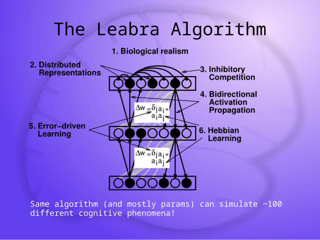
The Leabra Algorithm

Same algorithm (and mostly params) can simulate ~100 different cognitive phenomena!

Properties of Leabra Vision Model

Completely homogenous, more biological no separate S,C, SVM vs. RBF, etc

Learns at all levels of representation Each layer learns more complex and invariant

representations building on prior layer Fully bidirectional: top-down effects

Context, semantics, targets, ambiguity resolution… Full n-way classification in single model

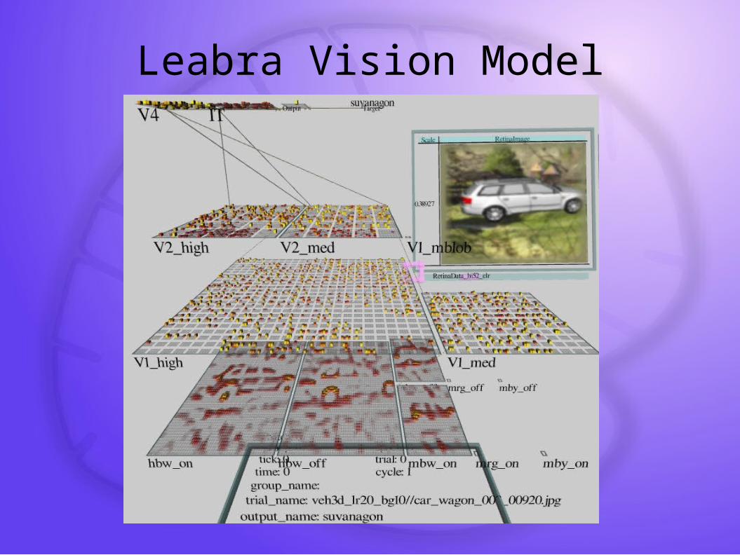
Leabra Vision Model

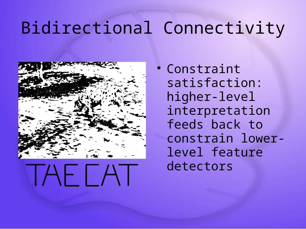
Bidirectional Connectivity

Constraint satisfaction: higher-level interpretation feeds back to constrain lower-level feature detectors

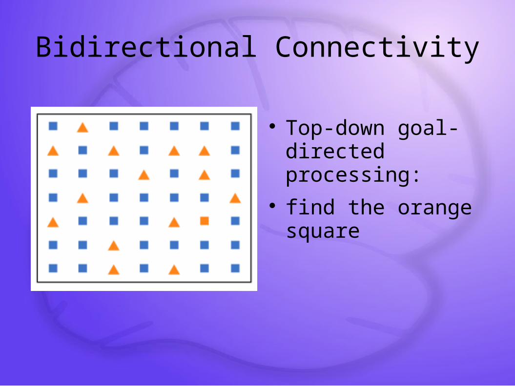
Bidirectional Connectivity

Top-down goal-directed processing:

find the orange square

3D Rendered Objects

Obtained from Google Sketchup Warehouse

Rendered in Emergent Virtual Environment using Coin3d (OpenInventor)

Part of major effort to systematically test object recognition system with easily parameterized datasets and large quantities of training and testing data.

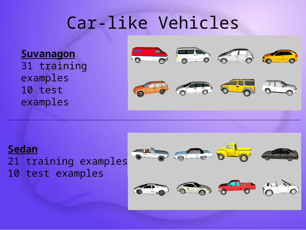
Car-like Vehicles

Suvanagon31 training examples10 test examples

Sedan21 training examples10 test examples

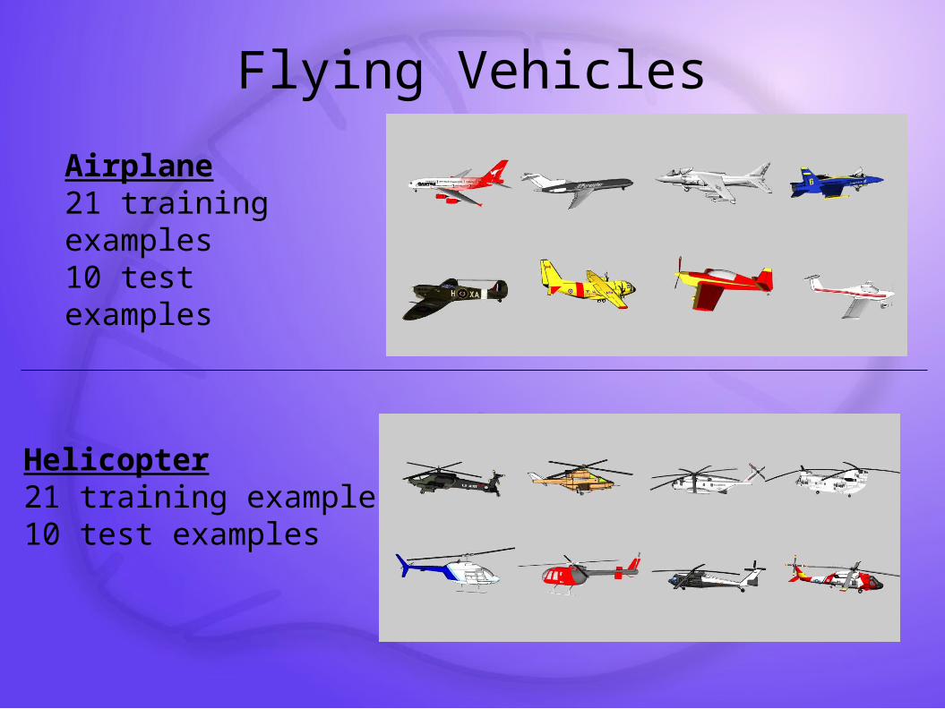
Flying Vehicles

Airplane21 training examples10 test examples

Helicopter21 training examples10 test examples

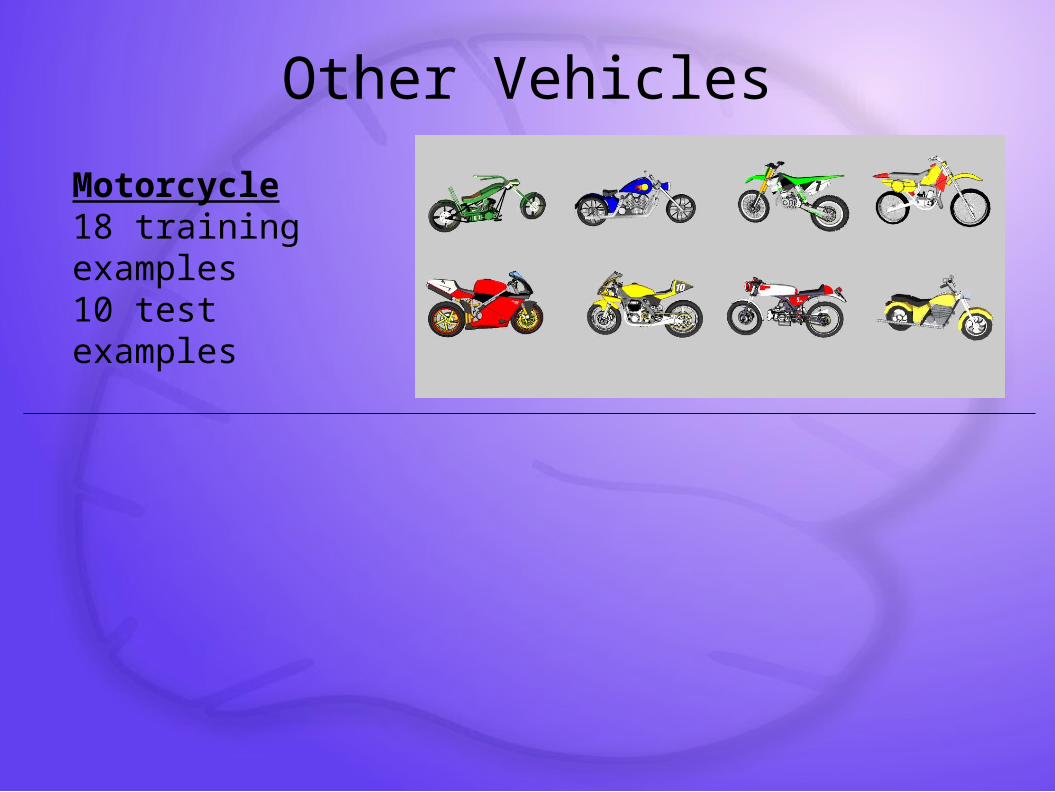
Other Vehicles

Motorcycle18 training examples10 test examples

Other Details

10 images per object rendered with different depth rotations and lighting:

Depth: left and right side-on images +/- 20deg rotation in depth plane

Lighting: position of overhead light varied randomly

As presented to network, affine transforms randomly applied:

scaling (25% size range)

translation (30% range of motion in each in-plane axis)

rotation in plane (14 deg total rotation range)

Testing: confidence-weighted voting over 7 random affine transforms per image.

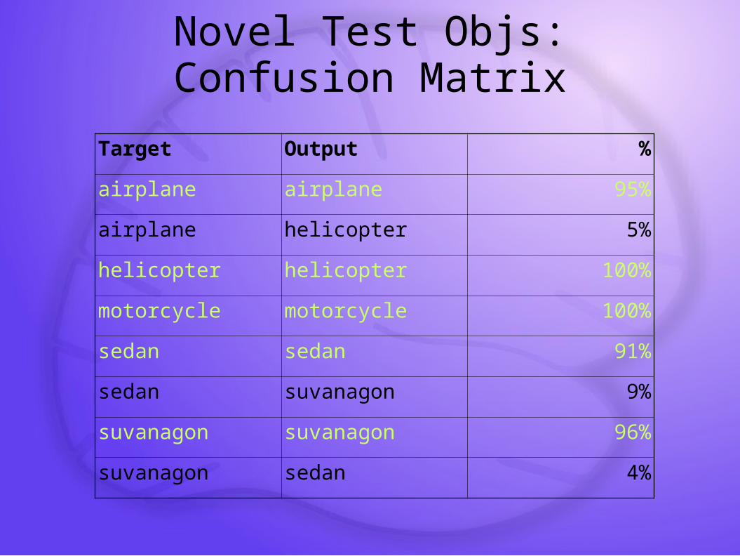
Novel Test Objs: Confusion Matrix

Target Output %

airplane airplane 95%

airplane helicopter 5%

helicopter helicopter 100%

motorcycle motorcycle 100%

sedan sedan 91%

sedan suvanagon 9%

suvanagon suvanagon 96%

suvanagon sedan 4%

Vehicles With Occlusion

10% width grey bar in middle of image: Airplane: 99% Helicopter: 38% (errs all airplane) Motorcycle: 70% Sedan: 88% Suvanagon: 93%

20% bar: Airplane: 99% Helicopter: 40% Motorcycle: 55% Sedan: 71% Suvanagon: 97%

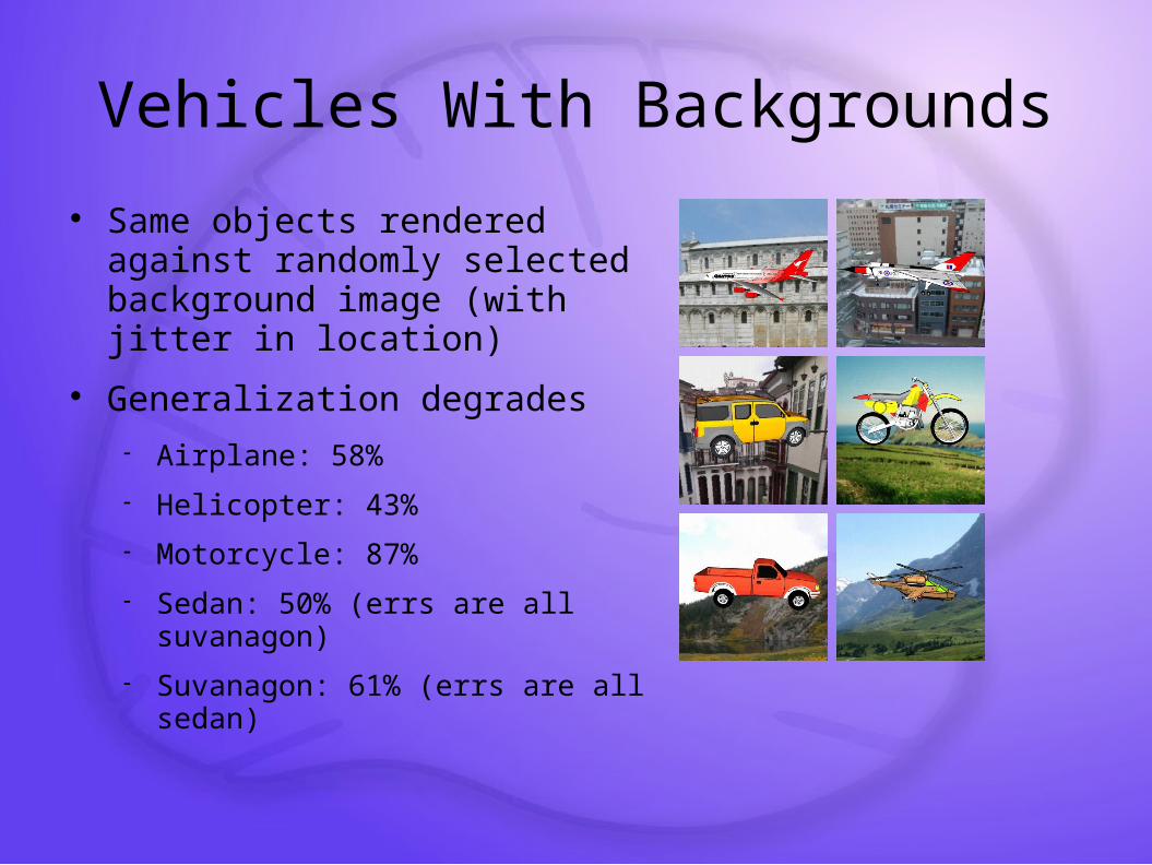
Vehicles With Backgrounds

Same objects rendered against randomly selected background image (with jitter in location)

Generalization degrades

Airplane: 58%

Helicopter: 43%

Motorcycle: 87%

Sedan: 50% (errs are all suvanagon)

Suvanagon: 61% (errs are all sedan)

Images from Video, Background Removed

Very simple first-pass motion-based filtering of video and subtraction of background to obtain vehicle images.

82 “sedan” images and 113 “suvanagon” images (same defn as 3d rendered objects), test on 12 of each, train on remainder

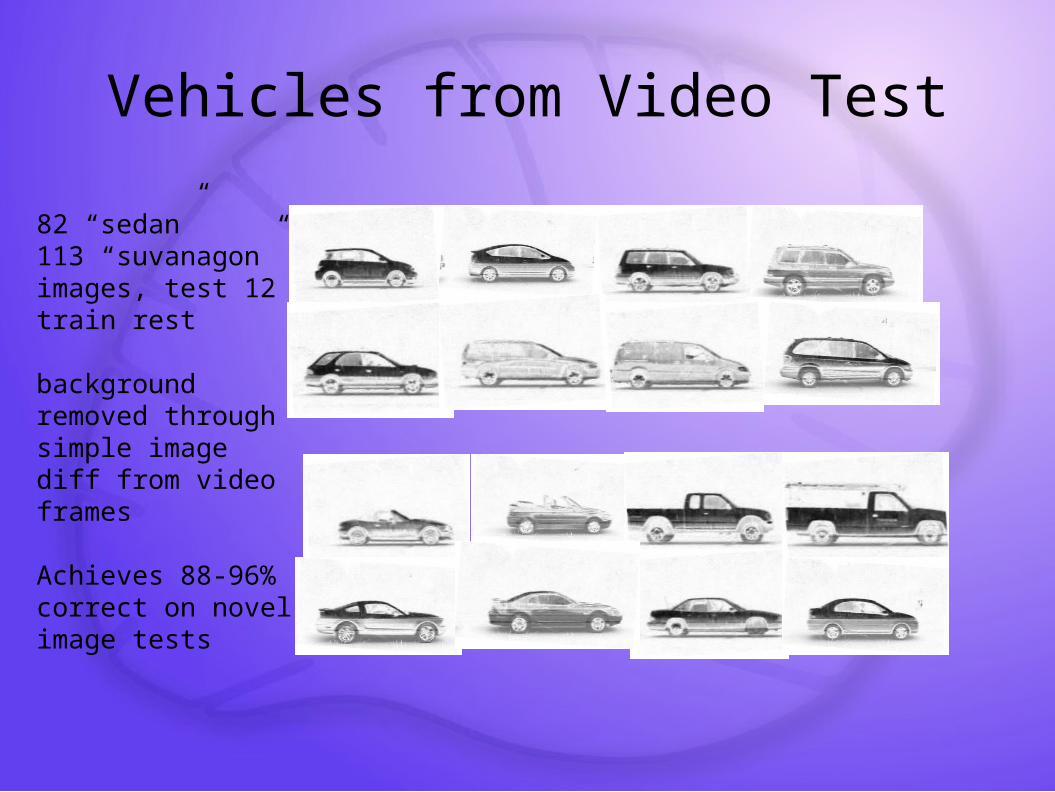
Vehicles from Video Test

82 “sedan”113 “suvanagon”images, test 12train rest

backgroundremoved throughsimple imagediff from videoframes

Achieves 88-96%correct on novelimage tests

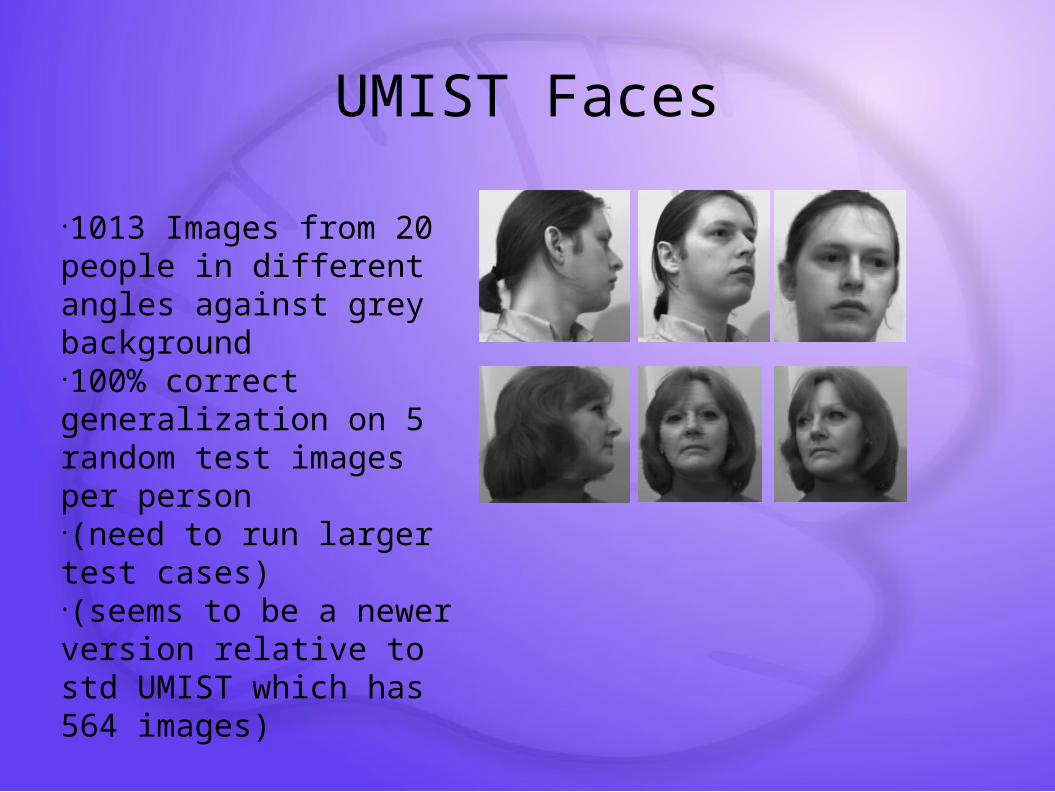
UMIST Faces

•1013 Images from 20 people in different angles against grey background•100% correct generalization on 5 random test images per person•(need to run larger test cases)•(seems to be a newer version relative to std UMIST which has 564 images)

MNIST Digits: Widely Used

•60K Training, 10K Testing•Best result is about .4% err•We get 2.1% err without any optimization

QuickTime™ and a decompressor

are needed to see this picture.

Caltech 101

QuickTime™ and a decompressor

are needed to see this picture.

Caltech 101: Flawed

QuickTime™ and a decompressor

are needed to see this picture.

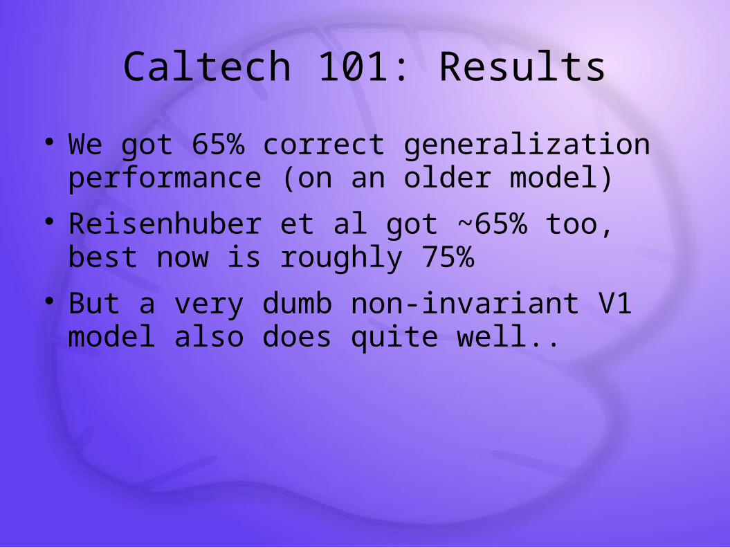
Caltech 101: Results

We got 65% correct generalization performance (on an older model)

Reisenhuber et al got ~65% too, best now is roughly 75%

But a very dumb non-invariant V1 model also does quite well..

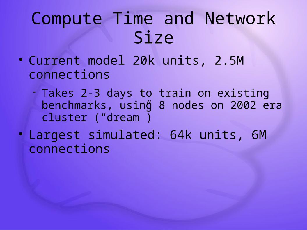
Compute Time and Network Size

Current model 20k units, 2.5M connections Takes 2-3 days to train on existing benchmarks,

using 8 nodes on 2002 era cluster (“dream”) Largest simulated: 64k units, 6M connections

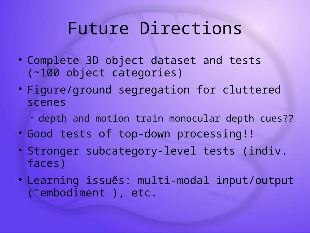
Future Directions

Complete 3D object dataset and tests (~100 object categories)

Figure/ground segregation for cluttered scenes depth and motion train monocular depth cues??

Good tests of top-down processing!! Stronger subcategory-level tests (indiv. faces) Learning issues: multi-modal input/output

(“embodiment”), etc.

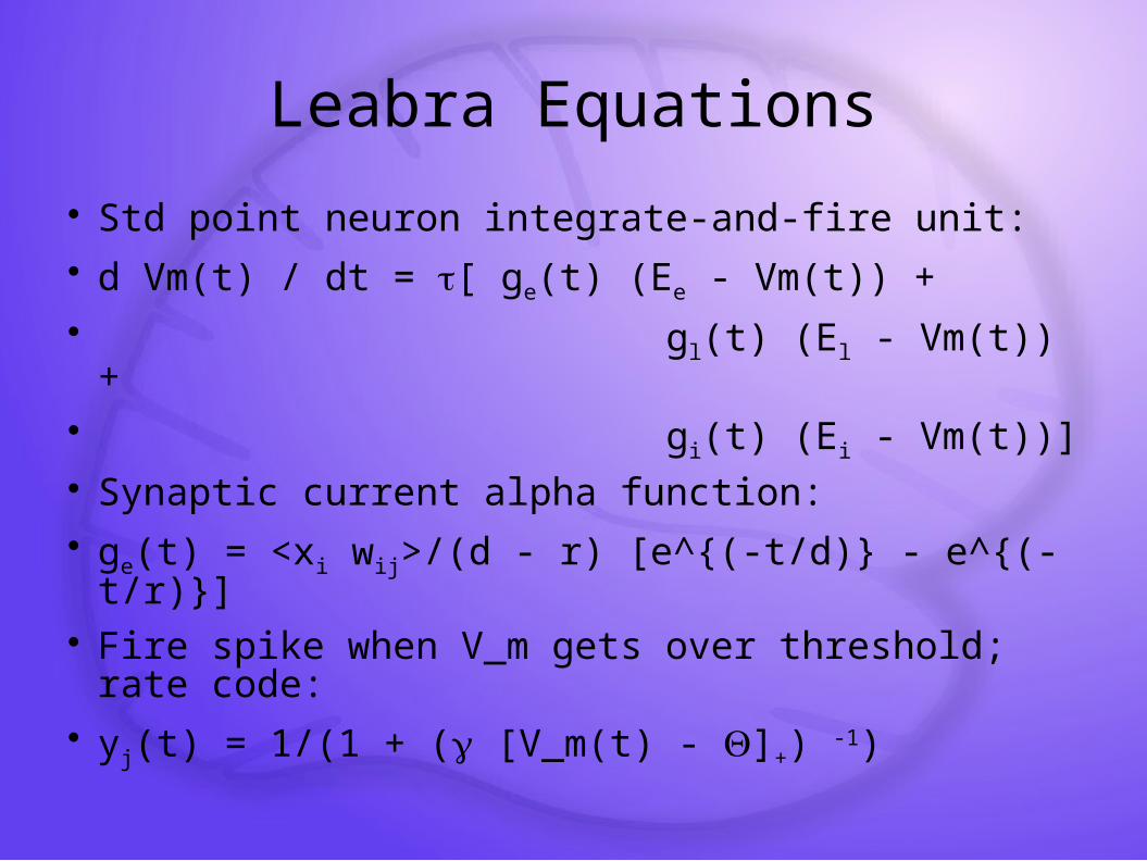
Leabra Equations

Std point neuron integrate-and-fire unit: d Vm(t) / dt = [ ge(t) (Ee - Vm(t)) + gl(t) (El - Vm(t)) + gi(t) (Ei - Vm(t))] Synaptic current alpha function: ge(t) = <xi wij>/(d - r) [e^{(-t/d)} - e^{(-t/r)}] Fire spike when V_m gets over threshold; rate code: yj(t) = 1/(1 + ( [V_m(t) - ]+) -1)

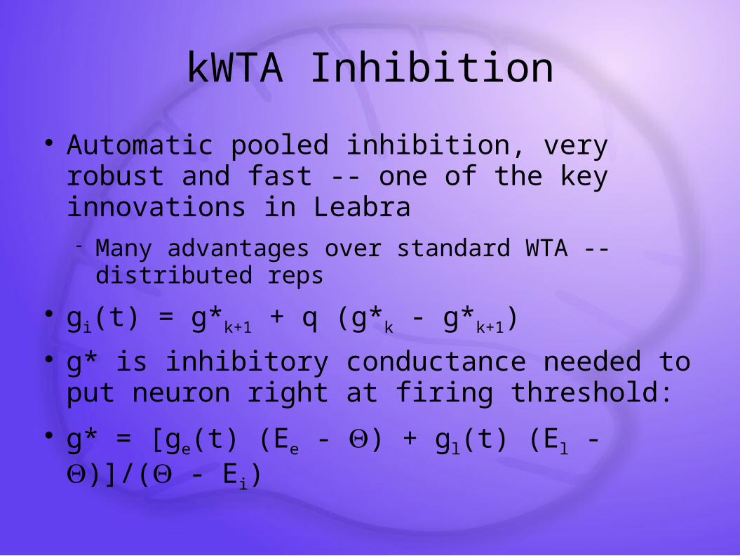
kWTA Inhibition

Automatic pooled inhibition, very robust and fast -- one of the key innovations in Leabra Many advantages over standard WTA -- distributed reps

gi(t) = g*k+1 + q (g*k - g*k+1) g* is inhibitory conductance needed to put neuron

right at firing threshold: g* = [ge(t) (Ee - ) + gl(t) (El - )]/( - Ei)

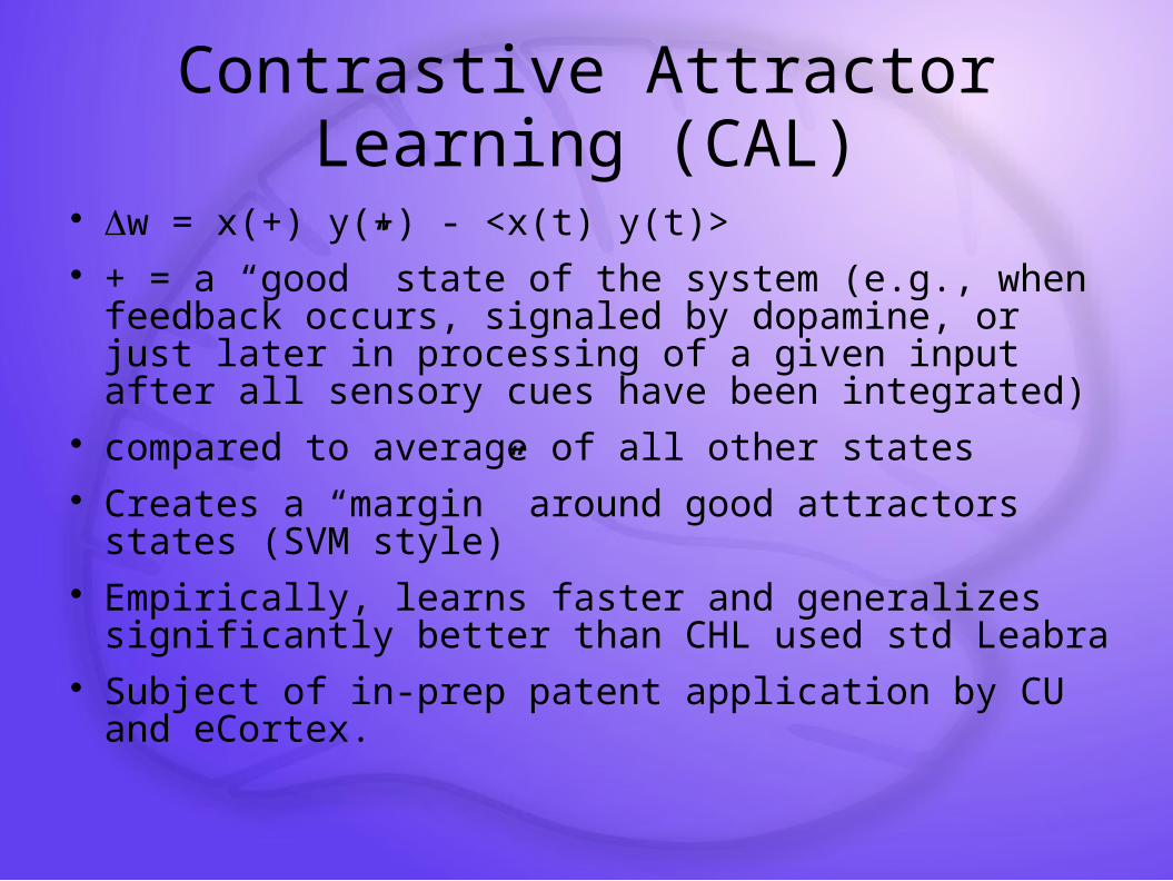
Contrastive Attractor Learning (CAL)

w = x(+) y(+) - <x(t) y(t)> + = a “good” state of the system (e.g., when feedback

occurs, signaled by dopamine, or just later in processing of a given input after all sensory cues have been integrated)

compared to average of all other states Creates a “margin” around good attractors states (SVM

style) Empirically, learns faster and generalizes significantly better

than CHL used std Leabra Subject of in-prep patent application by CU and eCortex.

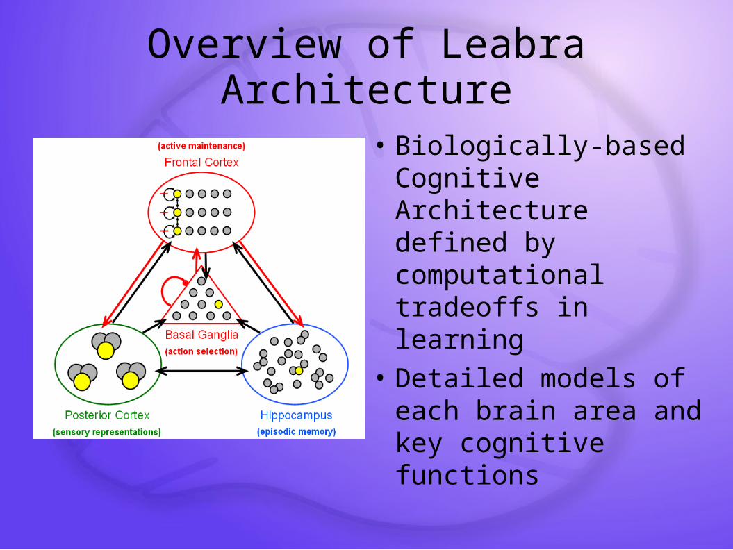
Overview of Leabra Architecture

• Biologically-based Cognitive Architecture defined by computational tradeoffs in learning

• Detailed models of each brain area and key cognitive functions