Embed Size (px)
Citation preview
Finance Stoch (2020) 24:1035–1082https://doi.org/10.1007/s00780-020-00431-6
The Leland–Toft optimal capital structure model underPoisson observations
Zbigniew Palmowski1 · José Luis Pérez2 ·Budhi Arta Surya3 · Kazutoshi Yamazaki4
Received: 6 April 2019 / Accepted: 26 March 2020 / Published online: 17 July 2020© The Author(s) 2020
Abstract This paper revisits the optimal capital structure model with endogenousbankruptcy, first studied by Leland (J. Finance 49:1213–1252, 1994) and Leland andToft (J. Finance 51:987–1019, 1996). Unlike in the standard case where sharehold-ers continuously observe the asset value and bankruptcy is executed instantaneouslywithout delay, the information of the asset value is assumed to be updated periodi-cally at the jump times of an independent Poisson process. Under a spectrally negativeLévy model, we obtain the optimal bankruptcy strategy and the corresponding capi-tal structure. A series of numerical studies provide an analysis of the sensitivity, withrespect to the observation frequency, of the optimal strategies, optimal leverage andcredit spreads.
Keywords Credit risk · Endogenous bankruptcy · Optimal capital structure ·Spectrally negative Lévy processes · Term structure of credit spreads
B K. [email protected]
J.L. Pé[email protected]
B.A. [email protected]
1 Faculty of Pure and Applied Mathematics, Wrocław University of Science and Technology,Wyb. Wyspianskiego 27, 50-370 Wrocław, Poland
2 Department of Probability and Statistics, Centro de Investigación en Matemáticas, A.C. CalleJalisco S/N, 36240 Guanajuato, Mexico
3 School of Mathematics and Statistics, Victoria University of Wellington, Gate 6, Kelburn PDE,Wellington 6140, New Zealand
4 Department of Mathematics, Faculty of Engineering Science, Kansai University, 3-3-35Yamate-cho, Suita-shi, Osaka 564-8680, Japan
1036 Z. Palmowski et al.
Mathematics Subject Classification (2010) 60G40 · 60G51 · 91G40
JEL Classification C61 · G32 · G33
1 Introduction
The study of capital structures dates back to the seminal work by Modigliani andMiller [45] which shows that in a frictionless economy, the value of a firm is in-variant to the choice of capital structures. While the Modigliani–Miller (MM) theoryis regarded as an effective starting point for research on capital structures and hasprovided valuable insights in the field, it is not directly applicable to businesses. Inreality, the selection of capital structures is not perfectly random. Instead, it dependssignificantly on factors such as industry type, country and corporate law. In the fieldof corporate finance, various approaches have been taken to explain how much debta firm should issue. A reasonable conclusion can be obtained only after challengingsome of the assumptions of the classical MM theory.
The trade-off theory is one well-known approach for the study of capital struc-tures. While various frictions may affect a firm’s decisions, bankruptcy costs and taxbenefits are believed to be the most important factors. By issuing debt, bankruptcycosts increase, while at the same time the firm can enjoy tax shields for coupon pay-ments to the bondholders. The trade-off theory states that firms issue the appropriatedebt to solve the trade-off between minimising bankruptcy costs and maximising taxbenefits. To formulate this optimisation problem, one needs an efficient and realisticway of modelling not only bankruptcy, but also tax benefits, which depend heavily onthe dynamics of the firm’s asset value. For more details on the trade-off theory and itsreview, see e.g. Frank and Goyal [27], Ju et al. [30] and Kraus and Litzenberger [32].
Classically, there are two models of bankruptcy in credit risk: the structural ap-proach and the reduced-form approach (see Bielecki and Rutkowski [12, Sects. 1.4,3.3, 3.6 and Part III]). The former, first proposed by Black and Cox [14], models thebankruptcy time as the first time the asset value goes below a fixed barrier. The lat-ter models it as the first jump epoch of a doubly stochastic process (known hereafteras a Cox process) where the jump rate is driven by another stochastic process. Bothapproaches were developed extensively in the 2000s and are now commonly usedthroughout the asset pricing and credit risk literature. An extension of the structuralapproach, which we call the excursion (Parisian) approach, models the bankruptcytime as the first instance in which the amount of time the asset value stays contin-uously below a threshold exceeds a given grace period. Motivated by the Parisianoption, this is sometimes called the Parisian ruin (see Chesney et al. [20]). In thecorporate finance literature, the approach has been used to model the reorganisationprocess (Chap. 11), as in Broadie et al. [16] or François and Morellec [26]. Here,reorganisation is undertaken whenever the asset value is below a threshold; althoughthere is a chance of recovering to return above the threshold, if the reorganisationtime exceeds the grace period, the firm is liquidated. For more information, see theliterature review in Sect. 1.3.

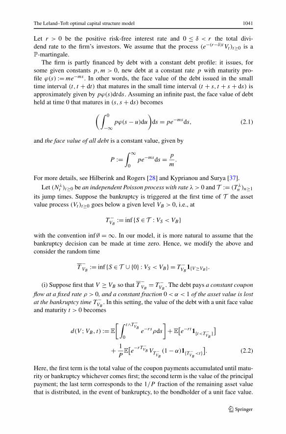
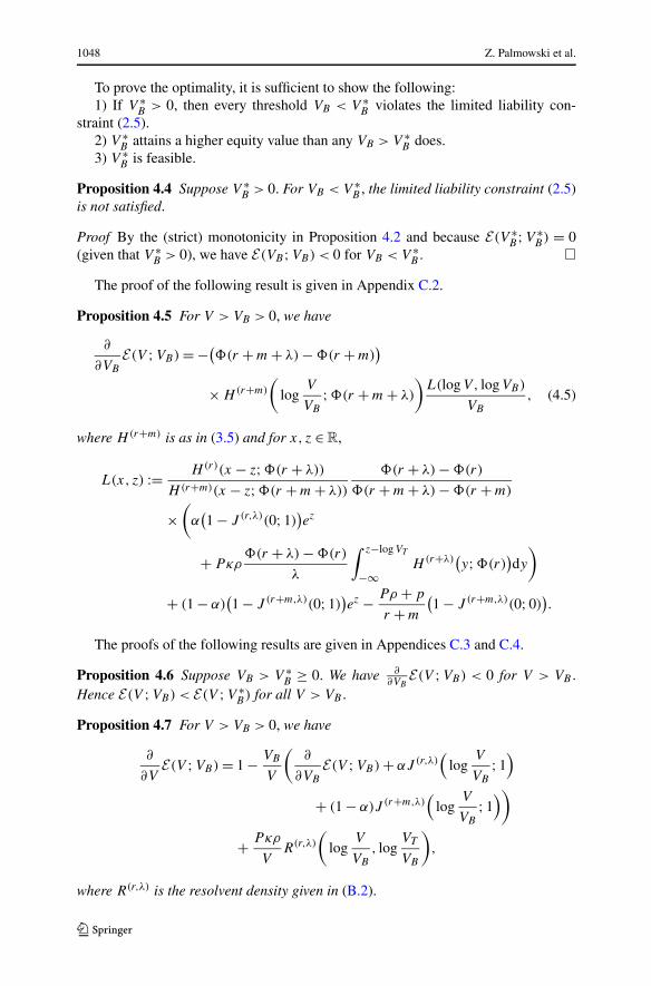
The Leland–Toft optimal capital structure model 1037
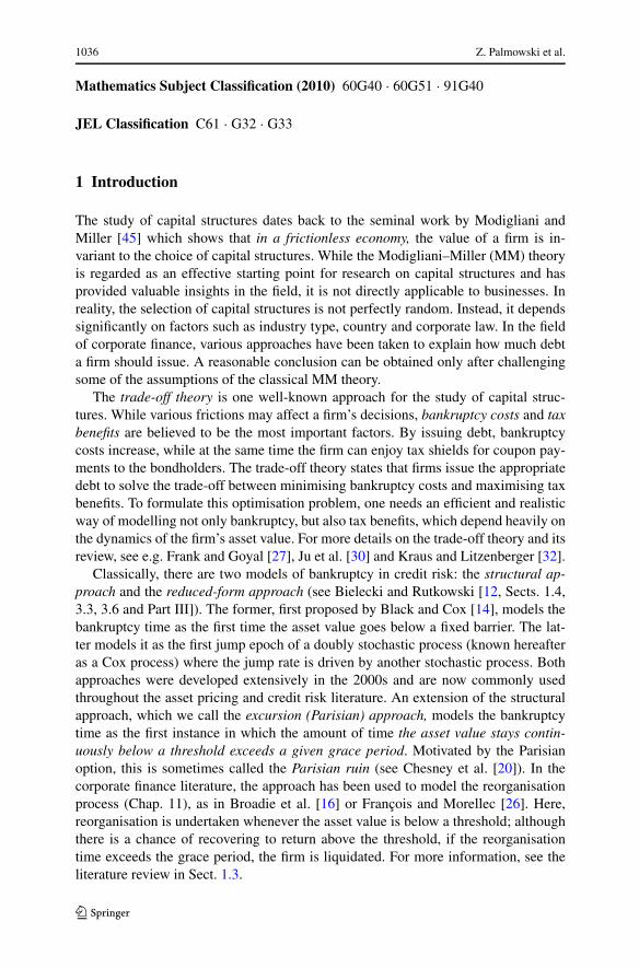
Fig. 1 Sample paths of theasset value (Vt )t≥0 (black lines)and (V λ
t )t≥0 (horizontal bluelines) along with the Poissonarrival times (T λ
n )n≥1 (indicatedby dotted vertical lines labelledTi on the x-axis). The red zone(0,VB) is given by the rectanglecolored in red. The asset valuesat bankruptcy and otherobservation times are indicatedby the red circle and bluetriangles, respectively. Here, thebankruptcy time corresponds toT λ
1 , but the asset value hascrossed VB before and thenrecovered back before T λ
1 . Note
that (V λt )t≥0 has a positive
jump at T λ6
1.1 A new model of bankruptcy
This paper considers the scenario where asset value information is updated only atepochs (T λ
n )n≥1 given by the jump times of a Poisson process (Nλt )t≥0 with fixed
rate λ. Given a bankruptcy barrier VB chosen by the equity holders, bankruptcy istriggered at the first update time where the asset process (Vt )t≥0 is below VB , i.e., at
inf{T λi : VT λ
i< VB}. (1.1)
This can also be written as the classical bankruptcy time
inf{t > 0 : V λt < VB} (1.2)
of the asset value if the latter is only updated at (T λn )n≥1, i.e., for
V λt := VT λ
Nλt
, t ≥ 0.
Here T λ
Nλt
is the most recent update time before t . In Fig. 1, we plot sample paths of
(Vt )t≥0, (V λt )t≥0, (T λ
n )n≥1 and the corresponding bankruptcy time.The bankruptcy model (1.1) is closely related to the reduced-form and excursion
approaches reviewed above:1) The bankruptcy time (1.1) is equivalent to the Parisian ruin with the (constant)
grace period replaced with an exponential time clock, the first epoch being the timespent continuously below VB for more than an independent exponential time. Formore details, see Appendix A.
2) It is also equivalent to the bankruptcy time in a reduced-form credit risk modelwhere the bankruptcy time is the first jump time of a Cox process with hazard rategiven by ht := λ1{Vt<VB }, t ≥ 0. As in Fig. 1, the region (0,VB) can be seen as the“red zone”; here, bankruptcy is triggered at rate λ, whereas in the “healthy zone”(VB,∞), this probability is negligible.
1038 Z. Palmowski et al.
There are several motivations for considering the bankruptcy strategy (1.1) for thestudy of capital structures.
First, in reality, it is not possible to continuously observe the accurate status of afirm and make bankruptcy decisions instantaneously. In addition, unlike in the caseof American option pricing for which computer programs can be set up to exerciseautomatically, in our case, information is acquired by humans. As observed in theliterature of rational inattention (Sims [52]), the amount of information a decisionmaker can capture and handle is limited, and instead they rationally decide to staywith imperfect information. Taking a bankruptcy decision requires complex informa-tion, and it is more realistic to assume that the information for the decision makers isupdated only at random discrete times. While they are expected to respond promptly,delays are inevitable and possibly have a significant impact on bankruptcy costs.
Second, the majority of the existing literature assumes continuous observation us-ing a continuous asset value process; in this case, the asset value at bankruptcy isin any event precisely VB . Unfortunately, it is unreasonable to assume that one canprecisely predict the asset value at bankruptcy, which is in reality random. The ran-domness can be realised by adding negative jumps to the process. We underline thatin our model, this randomness can also be achieved by any choice (continuous orcàdlàg) of the underlying process. See Fig. 6 in Sect. 6.
Third, this model generalises the classical model and allows more flexibility byhaving one more parameter λ. The classical structural model (with instantaneous liq-uidation upon downcrossing the barrier) corresponds to the case λ = ∞, and theno-bankruptcy model to the case λ = 0. With careful calibration of λ, the model canpotentially estimate the bankruptcy costs and tax benefits more precisely. Typically,for calibration, credit spread data is used. As shown in the numerical results (seeFig. 8), a variety of term structures can be achieved by choosing the value of λ.
Finally, thanks to the equivalence of our bankruptcy time with the classical bank-ruptcy time (1.2) of the process (V λ
t )t≥0, this research can be considered a contri-bution to the classical structural approach. Existing results featuring asset value pro-cesses with two-sided jumps are rather limited. However, we provide a new analyti-cally tractable case for (V λ
t )t≥0, containing two-sided jumps even when (Vt )t≥0 doesnot have positive jumps (see Fig. 1). By appropriately selecting the driving process(Vt )t≥0 as well as λ, it is possible to construct a wide range of stochastic processeswith two-sided jumps.
1.2 Contributions of the paper
Our model is built based on the seminal paper by Leland and Toft [39], with a featureof endogenous default. While Leland’s [38] framework is used more frequently andcertainly more mathematically tractable, its extension [39] more accurately capturesthe flow of debt financing by avoiding the use of perpetual bonds assumed in [38].
In addition, while the majority of papers in financial economics assume a geomet-ric Brownian motion for the asset value (Vt )t≥0, we follow the works of Hilberinkand Rogers [28], Kyprianou and Surya [37] and Surya and Yamazaki [54] and con-sider an exponential Lévy process with arbitrary negative jumps (i.e., a spectrallynegative Lévy process). Although it is more desirable to also allow positive jumps as
The Leland–Toft optimal capital structure model 1039
in Chen and Kou [19], as discussed in [28], negative jumps occur more frequently andeffectively model the downward risks. With the spectrally negative assumption, semi-explicit expressions of the equity value as well as the optimal bankruptcy thresholdare elicited, without focusing on a particular set of jump measures. Again, see thediscussion above on how our model is capable of modelling the two-sided jump casein the classical structural approach, even when a spectrally negative Lévy process isused for (Vt )t≥0. For a more general study of financial models using Lévy processes,the reader should refer to Cont and Tankov [21, Chaps. II and III].
To solve our problem, recent developments of the fluctuation theory of Lévy pro-cesses are utilised. First, the firm/debt/equity values are expressed in terms of theso-called scale functions, which exist for a general spectrally negative Lévy process.These permit direct computation of the optimal bankruptcy barrier and the corre-sponding firm/debt/equity values.
With these analytical results, a sequence of numerical experiments can be con-ducted. Here, to easily comprehend the impacts of the parameters describing theproblem, we use a (spectrally negative) hyperexponential jump diffusion (a mixtureof Brownian motion and i.i.d. hyperexponentially distributed jumps), for which thescale function can be written as a sum of exponential functions. The equity/debt/firmvalues can be written explicitly and the optimal bankruptcy barrier can be computedinstantaneously by a classical bisection method. The optimal capital structure is ob-tained by solving the two-stage optimisation problem as proposed in [39]. In addition,with numerical Laplace inversion, we also obtain the term structures of credit spreadsand the density/distribution of the bankruptcy time and the corresponding asset value.Because various numerical experiments have already been conducted in other papers,we focus here on analysing the impacts of the frequency of observation λ. We ver-ify the convergence to the classical case of [28, 37] and also observe monotonicity,with respect to λ, of the bankruptcy barrier, the firm value under the optimal capitalstructure, the optimal leverage and the credit spread.
1.3 Related literature
Before concluding this section, we review several relevant papers motivating ourproblem.
The most relevant paper, to the best of our knowledge, is François and Morellec[26] in which the authors model the reorganisation process (Chap. 11) using the ex-cursion approach with a deterministic grace period as described above. Broadie etal. [16] consider a similar model with an additional barrier for immediate liquida-tion upon crossing, whereas Moraux [46] considers a variant of [26] using the occu-pation time approach, in which distress level accumulates without being reset eachtime the asset process recovers to a healthy state. These papers are based on Leland[38], with perpetual bonds and asset values driven by geometric Brownian motionsfor mathematical tractability. However, computation of the solutions is significantlymore challenging than the classical structural approach and hence most papers relyon numerical approaches. In the present paper, on the other hand, semi-analytical so-lutions for a more general asset value process with jumps are obtained as a result ofthe use of Poisson arrival times for the update times.
1040 Z. Palmowski et al.
This paper is also motivated by Duffie and Lando [22] who model the asymme-try of information between firms and bond investors. The authors assume that bondinvestors cannot observe the firm’s assets directly and instead receive only periodicand imperfect accounting reports on the firm’s status. Under these assumptions, theauthors successfully explain the non-zero credit spread limit.
Regarding the study of Lévy processes observed at Poisson arrival times, there hasbeen substantial progress in the last few years. Recently, Albrecher and Ivanovs [1]investigated close links between Lévy processes observed continuously and periodi-cally. In results similar to those for the classical hitting time at a barrier, they foundthat the exit identities under periodic observation can be obtained if the Wiener–Hopffactorisation is known. In particular, when focusing on the spectrally one-sided case,these can be written in terms of the scale function. For the results of our paper, we usethe joint Laplace transform of the bankruptcy time (1.1) and the asset value at thattime, which is obtained in [2, 1]. In addition, we obtain the resolvent measure killedat the first Poisson downward passage time (1.1) for the computation of tax benefits.
Regarding the optimal stopping problems under Poisson observations, perpetualAmerican options have been studied by Dupuis and Wang [23] for the geometricBrownian motion case. This has recently been generalised to the Lévy case by Pérezand Yamazaki [49]. Several key studies have been performed on the application ofscale functions in optimal stopping in a continuous observation setting (see e.g. Aliliand Kyprianou [3], Avram et al. [7], Long and Zhang [43], Rodosthenous and Zhang[51] and Surya [53, Chap. 6]). The periodic observation model is more frequentlyused in the insurance community, in particular in the optimal dividend problem (seeAvanzi et al. [5, 6] and Noba et al. [47]).
To the best of our knowledge, this is the first attempt to introduce Poisson ob-servations in the problem of capital structures. We believe the techniques used inthis paper can be used similarly in related problems described above when a Poissonobservation scheme is introduced.
1.4 Organisation of the paper
The organisation of this paper is as follows. In Sect. 2, we present formally the mainproblem that we work on in this article. In Sect. 3, we compute the equity value usingthe scale function, and in Sect. 4, we identify the optimal barrier. Section 5 considersthe two-stage problem to obtain the optimal capital structure. Section 6 deals withnumerical examples confirming the theoretical results. Section 7 concludes the paper.Long proofs are deferred to Appendices B and C.
2 Problem formulation
Let (�,F ,P) be a complete probability space hosting a Lévy process X = (Xt )t≥0.The value of the firm’s asset is assumed to evolve according to an exponential Lévyprocess given, for the initial value V > 0, by
Vt := V eXt , t ≥ 0.
The Leland–Toft optimal capital structure model 1041
Let r > 0 be the positive risk-free interest rate and 0 ≤ δ < r the total divi-dend rate to the firm’s investors. We assume that the process (e−(r−δ)tVt )t≥0 is aP-martingale.
The firm is partly financed by debt with a constant debt profile: it issues, forsome given constants p,m > 0, new debt at a constant rate p with maturity pro-file ϕ(s) := me−ms . In other words, the face value of the debt issued in the smalltime interval (t, t + dt) that matures in the small time interval (t + s, t + s + ds) isapproximately given by pϕ(s)dtds. Assuming an infinite past, the face value of debtheld at time 0 that matures in (s, s + ds) becomes
(∫ 0
−∞pϕ(s − u)du
)ds = pe−msds, (2.1)
and the face value of all debt is a constant value, given by
P :=∫ ∞
0pe−msds = p
m.
For more details, see Hilberink and Rogers [28] and Kyprianou and Surya [37].
Let (Nλt )t≥0 be an independent Poisson process with rate λ > 0 and T := (T λ
n )n≥1
its jump times. Suppose the bankruptcy is triggered at the first time of T the assetvalue process (Vt )t≥0 goes below a given level VB > 0, i.e., at
T −VB
:= inf {S ∈ T : VS < VB}
with the convention inf∅ = ∞. In our model, it is more natural to assume that thebankruptcy decision can be made at time zero. Hence, we modify the above andconsider the random time
T−VB
:= inf {S ∈ T ∪ {0} : VS < VB} = T −VB
1{V ≥VB }.
(i) Suppose first that V ≥ VB so that T−VB
= T −VB
. The debt pays a constant coupon
flow at a fixed rate ρ > 0, and a constant fraction 0 < α < 1 of the asset value is lostat the bankruptcy time T −
VB. In this setting, the value of the debt with a unit face value
and maturity t > 0 becomes
d(V ;VB, t) := E
[∫ t∧T −VB
0e−rsρds
]+E
[e−rt1{t<T −
VB}]
+ 1
PE
[e−rT −
VB VT −VB
(1 − α)1{T −VB
<t}]. (2.2)
Here, the first term is the total value of the coupon payments accumulated until matu-rity or bankruptcy whichever comes first; the second term is the value of the principalpayment; the last term corresponds to the 1/P fraction of the remaining asset valuethat is distributed, in the event of bankruptcy, to the bondholder of a unit face value.
1042 Z. Palmowski et al.
Integrating this, the total value of debt becomes, by (2.1) and Fubini’s theorem,
D(V ;VB) :=∫ ∞
0pe−mtd(V ;VB, t)dt
= E
[∫ T −VB
0e−(r+m)t (Pρ + p)dt
]
+E[e−(r+m)T −
VB VT −VB
(1 − α)1{T −VB
<∞}].
Regarding the value of the firm, it is assumed that there is a corporate tax rate κ > 0and its (full) rebate on coupon payments is gained if and only if Vt ≥ VT for somegiven cut-off level VT ≥ 0 (for the case VT = 0, it enjoys the benefit at all times).Based on the trade-off theory (see e.g. Brealey and Myers [15, Chap. 9]), the firmvalue becomes the sum of the asset value and total value of tax benefits less the valueof loss at bankruptcy and is given by
V(V ;VB) := V +E
[∫ T −VB
0e−rt1{Vt≥VT }Pκρdt
]− αE
[e−rT −
VB VT −VB
1{T −VB
<∞}].
(ii) Suppose now V < VB so that T−VB
= 0. Then by setting T −VB
= 0 in the com-putations in (i), we obtain
D(V ;VB) = V(V ;VB) = (1 − α)V . (2.3)
The problem is to find an optimal bankruptcy level VB ≥ 0 that maximises theequity value
E(V ;VB) := V(V ;VB) −D(V ;VB), (2.4)
subject to the limited liability constraint
E(V ;VB) ≥ 0, V ≥ VB, (2.5)
if such a level exists. Here, VB = 0 means that it is never optimal to go bankrupt withthe limited liability constraint satisfied for all V > 0. Note that when V < VB , then(2.3) gives E(V ;VB) = 0.
3 Computation of the equity value
Suppose from now on that (Xt )t≥0 is a spectrally negative Lévy process, that is,a Lévy process without positive jumps. We denote by
ψ(θ) := logE[eθX1], θ ≥ 0, (3.1)
its Laplace exponent with the right inverse
�(q) := sup{s ≥ 0 : ψ(s) = q}, q ≥ 0. (3.2)
The Leland–Toft optimal capital structure model 1043
3.1 Scale functions
The starting point of the whole analysis is introducing the so-called q-scale functionW(q)(x), with q ≥ 0 and x ∈ R. It features invariably in almost all known fluctua-tion identities of spectrally negative Lévy processes; see Zolotarev [56] and Takács[55, Part 4] for the origin of this function. See also Kuznetsov et al. [35] and Kypri-anou and Surya [37] for a detailed review.
Fix q ≥ 0. The q-scale function W(q) is the mapping from R to [0,∞) that takesvalue zero on the negative half-line, while on the positive half-line it is a continuousand strictly increasing function with the Laplace transform
∫ ∞
0e−θxW(q)(x)dx = 1
ψ(θ) − q, θ > �(q). (3.3)
Define also the second scale function
Z(q)(x; θ) := eθx
(1 + (
q − ψ(θ)) ∫ x
0e−θzW(q)(z)dz
), x ∈R, θ ≥ 0.
In particular, for x ∈R, we let Z(q)(x) := Z(q)(x;0), and for λ > 0,
Z(q)(x;�(q + λ)
) = e�(q+λ)x
(1 − λ
∫ x
0e−�(q+λ)zW(q)(z)dz
).
In the next section, we shall see that the equity value (2.4) can be written in terms ofthe scale functions W(q) and Z(q).
3.2 Related fluctuation identities
For y ∈ R, let Py be the conditional probability under which the initial value of thespectrally negative Lévy process is X0 = y.
Following equation (4.5) in [37] (see also Emery [25] and Avram et al.[8, Eq. (3.19)]), the joint Laplace transform of the first passage time
τ−0 := inf{t ≥ 0 : Xt < 0} (3.4)
and Xτ−0
is given by the identity
H(q)(y; θ) := Ey
[e−qτ−
0 +θXτ−0 1{τ−
0 <∞}] = Z(q)(y; θ) − ψ(θ) − q
θ − �(q)W(q)(y), (3.5)
where y ∈ R, θ ≥ 0 and q ≥ 0. Similar results have been obtained for the Poissonobservation case. Recall that T := (T λ
n )n≥1 is the set of jump times of an independentPoisson process. We define
T −z := inf{S ∈ T : XS < z}, z ∈ R. (3.6)
1044 Z. Palmowski et al.
By equation (14) of Theorem 3.1 in Albrecher et al. [2], for θ ≥ 0 and y ∈ R,
J (q,λ)(y; θ)
:= Ey
[e−qT −
0 +θXT
−0 1{T −
0 <∞}]
= λ
λ + q − ψ(θ)
(Z(q)(y; θ) − Z(q)(y;�(q + λ))
ψ(θ) − q
λ
�(q + λ) − �(q)
θ − �(q)
)
=(
1 − ψ(θ) − q
θ − �(q)
�(λ + q) − θ
λ + q − ψ(θ)
)Z(q)(y; θ)
− ψ(θ) − q
θ − �(q)
�(λ + q) − �(q)
λ + q − ψ(θ)
(Z(q)
(y;�(λ + q)
) − Z(q)(y; θ)). (3.7)
Remark 3.1 1) We have
J (q,λ)(0;1) = λ
λ + q − ψ(1)− ψ(1) − q
λ + q − ψ(1)
�(q + λ) − �(q)
1 − �(q)
= 1 − ψ(1) − q
λ + q − ψ(1)
�(q + λ) − 1
1 − �(q)> 0,
J (q,λ)(0;0) = λ
λ + q− q
λ + q
�(q + λ) − �(q)
�(q)= 1 − q
λ + q
�(q + λ)
�(q)> 0,
where the positivity holds by the probabilistic expression of J (q,λ) as in (3.7).2) We have
J (q,λ)(y; θ) < 1, q > 0, θ ≥ 0, y ∈ R. (3.8)
To see this, by the memoryless property of the exponential distribution, we can write,for some independent exponential random variable eλ, the first observation time atwhich X is below zero as τ−
0 + eλ, and hence T −0 is bounded from below by an
exponential random variable. In addition, we must have XT −
0≤ 0 Py -a.s. and hence
we have (3.8).
In order to write the equity value, we obtain an expression for
(r,λ)(y, z) := Ey
[∫ T −z
0e−rt1{Xt≥logVT }dt
], y, z ∈R. (3.9)
In Appendix B, we obtain the resolvent measure killed at T −z and the following result
as a corollary.

The Leland–Toft optimal capital structure model 1045
Proposition 3.2 Fix y, z ∈R. For VT > 0, we have
(r,λ)(y, z) = Z(r)(y − z;�(r + λ)
)�(r + λ) − �(r)
λ
×(
1
�(r)Z(r+λ)
(z − logVT ;�(r)
) − λ
�(r)W
(r+λ)(z − logVT )
)
− W(r+λ)
(y − logVT )1{z>logVT } − W(r)
(y − logVT )1{z≤logVT }
+ λ1{z>logVT }∫ y−z
0W(r)(y − z − u)W
(r+λ)(u + z − logVT )du,
where W(q)
(y) := ∫ y
0 W(q)(u)du for all q > 0 and y ∈ R. For VT = 0, we have
(r,λ)(y, z) = (1 − J (r,λ)(y − z;0))/r .
3.3 Expression for the equity value in terms of the scale function
Using the identities in Sect. 3.2, the equity value (2.4) can be written as follows. Here,we focus on the case VB > 0. The case VB = 0 (for which, as we shall see, only thecase VT = 0 needs to be considered) is given later in (4.4).
First, (3.7) gives, for q = r and q = r + m,
E[e−qT −
VB VT −VB
1{T −VB
<∞}] = VBJ (q,λ)
(log
V
VB
;1
),
E[e−qT −
VB 1{T −VB
<∞}] = J (q,λ)
(log
V
VB
;0
).
In addition, by (3.9),
E
[∫ T −VB
0e−rt1{Vt≥VT }dt
]= (r,λ)(logV, logVB).
Hence we can write
D(V ;VB) = Pρ + p
r + m
(1 − J (r+m,λ)
(log
V
VB
;0))
+ (1 − α)VBJ (r+m,λ)
(log
V
VB
;1
),
V(V ;VB) = V + Pκρ (r,λ)(logV, logVB) − αVBJ (r,λ)
(log
V
VB
;1
), (3.10)

1046 Z. Palmowski et al.
and therefore, by taking their difference, the equity value is
E(V ;VB) = V + Pκρ (r,λ)(logV, logVB) − αVBJ (r,λ)
(log
V
VB
;1
)
− Pρ + p
r + m
(1 − J (r+m,λ)
(log
V
VB
;0))
− (1 − α)VBJ (r+m,λ)
(log
V
VB
;1
). (3.11)
4 Optimal barrier
Having identified the equity value E(V ;VB) in (3.11), we are ready to find the optimalbarrier V ∗
B that maximises it. Our objective in this paper is to show that the optimalbarrier is V ∗
B such that
E(V ∗B ;V ∗
B) = 0, (4.1)
if it exists, where by (3.11) and Remark 3.1, 1), for VB > 0,
E(VB;VB) = VB + Pκρ (r,λ)(logVB, logVB) − αVBJ (r,λ)(0;1)
− Pρ + p
r + m
(1 − J (r+m,λ)(0;0)
) − (1 − α)VBJ (r+m,λ)(0;1)
= VB
(1 − αJ (r,λ)(0;1) − (1 − α)J (r+m,λ)(0;1)
)
+ Pκρ (r,λ)(logVB, logVB) − Pρ + p
λ + r + m
�(r + m + λ)
�(r + m). (4.2)
4.1 Existence
We first exhibit a condition for the existence of V ∗B satisfying (4.1). To this end, we
show the following result; the proof is given in Appendix C.1.
Lemma 4.1 The mapping z → (r,λ)(z, z) is nondecreasing on R with the limit
limz↓−∞ (r,λ)(z, z) =
{0 if VT > 0,
1λ+r
�(r+λ)�(r)
if VT = 0.
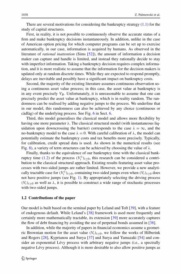
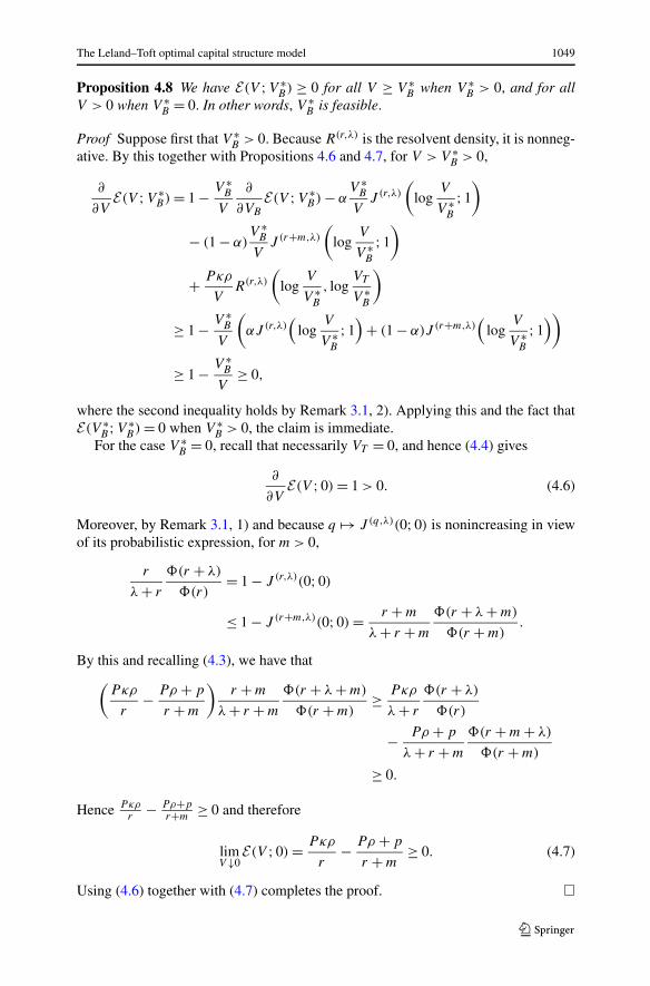
This lemma leads to the following proposition. For numerical illustration, seeFig. 2.
Proposition 4.2 The mapping VB → E(VB;VB) is strictly increasing on (0,∞) withthe limits
limVB↓0
E(VB;VB) =⎧⎨⎩
− Pρ+pλ+r+m
�(r+m+λ)�(r+m)
if VT > 0,
Pκρλ+r
�(r+λ)�(r)
− Pρ+pλ+r+m
�(r+m+λ)�(r+m)
if VT = 0,
limVB↑∞E(VB;VB) = ∞.

The Leland–Toft optimal capital structure model 1047
Fig. 2 Plots of VB → E(VB ;VB) for VT = 0,10,20, . . . ,100. Solid lines are for the case VT = 0 anddotted lines for the other cases. The points at V ∗
Bare indicated by circles. The left plot is based on the
parameter set in Case B in Sect. 6 (except VT ), and achieves V ∗B
> 0 for all cases. The right plot is basedon the same parameters except that we set κ = 0.9999, m = 10, ρ = 0.2 and λ = 0.1 to achieve V ∗
B= 0
when VT = 0
Proof From Remark 3.1, 2), we have 1 − αJ (r,λ)(0;1) − (1 − α)J (r+m,λ)(0;1) > 0.By this, Lemma 4.1 and because z → (r,λ)(z, z) is nondecreasing and bounded, theclaim is immediate in view of the second equality in (4.2). �
Now by Proposition 4.2, we define the candidate optimal threshold V ∗B formally
as follows:1) If VT > 0 or if VT = 0 with Pκρ
λ+r�(r+λ)�(r)
− Pρ+pλ+r+m
�(r+m+λ)�(r+m)
< 0, we set V ∗B > 0
such that E(V ∗B ;V ∗
B) = 0, whose existence and uniqueness hold by Proposition 4.2.2) If VT = 0 with
Pκρ
λ + r
�(r + λ)
�(r)− Pρ + p
λ + r + m
�(r + m + λ)
�(r + m)≥ 0, (4.3)
we set V ∗B = 0.
The debt/firm/equity values for the case V ∗B > 0 can be computed by (3.10) and
(3.11). For the case V ∗B = 0 where necessarily VT = 0, we have, for all V > 0,
D(V ;0) = E
[∫ ∞
0e−(r+m)t (Pρ + p)dt
]= Pρ + p
r + m,
V(V ;0) = V +E
[∫ ∞
0e−rtP κρdt
]= V + Pκρ
r
and therefore
E(V ;0) = V + Pκρ
r− Pρ + p
r + m. (4.4)
4.2 Optimality
In the rest of this section, we show the following one of our main results.
Theorem 4.3 The barrier V ∗B is optimal for the problem of maximising (2.4) subject
to (2.5).
1048 Z. Palmowski et al.
To prove the optimality, it is sufficient to show the following:1) If V ∗
B > 0, then every threshold VB < V ∗B violates the limited liability con-
straint (2.5).2) V ∗
B attains a higher equity value than any VB > V ∗B does.
3) V ∗B is feasible.
Proposition 4.4 Suppose V ∗B > 0. For VB < V ∗
B , the limited liability constraint (2.5)is not satisfied.
Proof By the (strict) monotonicity in Proposition 4.2 and because E(V ∗B ;V ∗
B) = 0(given that V ∗
B > 0), we have E(VB;VB) < 0 for VB < V ∗B . �
The proof of the following result is given in Appendix C.2.
Proposition 4.5 For V > VB > 0, we have
∂
∂VB
E(V ;VB) = −(�(r + m + λ) − �(r + m)
)
× H(r+m)
(log
V
VB
;�(r + m + λ)
)L(logV, logVB)
VB
, (4.5)
where H(r+m) is as in (3.5) and for x, z ∈R,
L(x, z) := H(r)(x − z;�(r + λ))
H(r+m)(x − z;�(r + m + λ))
�(r + λ) − �(r)
�(r + m + λ) − �(r + m)
×(
α(1 − J (r,λ)(0;1)
)ez
+ Pκρ�(r + λ) − �(r)
λ
∫ z−logVT
−∞H(r+λ)
(y;�(r)
)dy
)
+ (1 − α)(1 − J (r+m,λ)(0;1)
)ez − Pρ + p
r + m
(1 − J (r+m,λ)(0;0)
).
The proofs of the following results are given in Appendices C.3 and C.4.
Proposition 4.6 Suppose VB > V ∗B ≥ 0. We have ∂
∂VBE(V ;VB) < 0 for V > VB .
Hence E(V ;VB) < E(V ;V ∗B) for all V > VB .
Proposition 4.7 For V > VB > 0, we have
∂
∂VE(V ;VB) = 1 − VB
V
(∂
∂VB
E(V ;VB) + αJ (r,λ)(
logV
VB
;1)
+ (1 − α)J (r+m,λ)(
logV
VB
;1))
+ Pκρ
VR(r,λ)
(log
V
VB
, logVT
VB
),
where R(r,λ) is the resolvent density given in (B.2).
The Leland–Toft optimal capital structure model 1049
Proposition 4.8 We have E(V ;V ∗B) ≥ 0 for all V ≥ V ∗
B when V ∗B > 0, and for all
V > 0 when V ∗B = 0. In other words, V ∗
B is feasible.
Proof Suppose first that V ∗B > 0. Because R(r,λ) is the resolvent density, it is nonneg-
ative. By this together with Propositions 4.6 and 4.7, for V > V ∗B > 0,
∂
∂VE(V ;V ∗
B) = 1 − V ∗B
V
∂
∂VB
E(V ;V ∗B) − α
V ∗B
VJ (r,λ)
(log
V
V ∗B
;1
)
− (1 − α)V ∗
B
VJ (r+m,λ)
(log
V
V ∗B
;1
)
+ Pκρ
VR(r,λ)
(log
V
V ∗B
, logVT
V ∗B
)
≥ 1 − V ∗B
V
(αJ (r,λ)
(log
V
V ∗B
;1)
+ (1 − α)J (r+m,λ)(
logV
V ∗B
;1))
≥ 1 − V ∗B
V≥ 0,
where the second inequality holds by Remark 3.1, 2). Applying this and the fact thatE(V ∗
B ;V ∗B) = 0 when V ∗
B > 0, the claim is immediate.For the case V ∗
B = 0, recall that necessarily VT = 0, and hence (4.4) gives
∂
∂VE(V ;0) = 1 > 0. (4.6)
Moreover, by Remark 3.1, 1) and because q → J (q,λ)(0;0) is nonincreasing in viewof its probabilistic expression, for m > 0,
r
λ + r
�(r + λ)
�(r)= 1 − J (r,λ)(0;0)
≤ 1 − J (r+m,λ)(0;0) = r + m
λ + r + m
�(r + λ + m)
�(r + m).
By this and recalling (4.3), we have that(
Pκρ
r− Pρ + p
r + m
)r + m
λ + r + m
�(r + λ + m)
�(r + m)≥ Pκρ
λ + r
�(r + λ)
�(r)
− Pρ + p
λ + r + m
�(r + m + λ)
�(r + m)
≥ 0.
Hence Pκρr
− Pρ+pr+m
≥ 0 and therefore
limV ↓0
E(V ;0) = Pκρ
r− Pρ + p
r + m≥ 0. (4.7)
Using (4.6) together with (4.7) completes the proof. �
1050 Z. Palmowski et al.
Proof of Theorem 4.3 By Propositions 4.4, 4.6 and 4.8, the proof is complete. �
Remark 4.9 Intuitively, as λ → ∞, the optimal barrier is expected to converge to thatin the classical case as in Kyprianou and Surya [37]. In order to confirm this assertion,we provide the following result; its proof is deferred to Appendix C.5.
Lemma 4.10 Suppose VT > 0 and let VB ≥ 0 be fixed. We have
limλ→∞
λ + r + m
�(λ + r + m)E(VB;VB) = VB
(α
ψ(1) − r
1 − �(r)+ (1 − α)
ψ(1) − (r + m)
1 − �(r + m)
)
+ Pκρ
�(r)
((VB
VT
)�(r) ∧ 1
)− Pρ + p
�(r + m). (4.8)
This is consistent with the identity (3.26) in [37], where the optimal bankruptcylevel is such that the right-hand side of (4.8) vanishes.
5 Two-stage problem
We now obtain the optimal leverage by solving the two-stage problem as studiedby Chen and Kou [19], Leland [38] and Leland and Toft [39], where the final goalis to choose P that maximises the firm’s value V . For fixed V > 0, the problem isformulated as
maxP
V(V ;V ∗
B(P ),P)
(5.1)
where we emphasise the dependence of V and V ∗B on P .
In this two-stage problem, it is worth investigating the shape of V(V ;V ∗B(P ),P )
with respect to P to confirm whether it has a unique maximiser. Chen and Kou[19] verified the concavity in the continuous observation case with a double jump-diffusion as the underlying model and the assumption that VT = 0.
In this section, we show in the periodic observation setting the concavity for thecase when VT = 0 and the following assumption is satisfied.
Assumption 5.1 The Lévy measure � of the dual process −X has a completelymonotone density, i.e., � has a density π whose nth derivative π(n) exists for alln ≥ 1 and satisfies
(−1)nπ(n)(x) ≥ 0, x > 0.
Important examples satisfying Assumption 5.1 include (the spectrally negativeversions of) the hyperexponential jump-diffusion (as a generalisation of [19]), thevariance gamma process (Madan and Seneta [44]), the CGMY process (Carr etal. [18]), as well as meromorphic Lévy processes (Kuznetsov et al. [34]).
To show this claim, we first show the following property.
The Leland–Toft optimal capital structure model 1051
Lemma 5.2 Under Assumption 5.1, the mapping x → H(r)(x;�(r +λ)) is decreas-ing.
Proof For the completely monotone case, it is known from Loeffen [41, Theorem 2]that the scale function admits the form
W(r)(x) = �′(r)e�(r)x −∫ ∞
0e−xtμ(r)(dt), x ≥ 0,
for some finite measure μ(r). Substituting this and using Fubini’s theorem, we get
Z(r)(x;�(r + λ)
)
= e�(r+λ)x
(1 − λ
∫ x
0e−�(r+λ)z
(�′(r)e�(r)z −
∫ ∞
0e−ztμ(r)(dt)
)dz
)
= e�(r+λ)x
(1 − λ
(�′(r)1 − e−(�(r+λ)−�(r))x
�(r + λ) − �(r)
−∫ ∞
0
∫ x
0e−z(t+�(r+λ))dzμ(r)(dt)
))
= e�(r+λ)x − λ
(�′(r)e
�(r+λ)x − e�(r)x
�(r + λ) − �(r)−
∫ ∞
0
e�(r+λ)x − e−tx
t + �(r + λ)μ(r)(dt)
).
Now substituting the above expressions in (3.5), we have
H(r)(x;�(r + λ)
)
= Z(r)(x;�(r + λ)
) − λ
�(r + λ) − �(r)W(r)(x)
= e�(r+λ)x − λ
(�′(r)e
�(r+λ)x − e�(r)x
�(r + λ) − �(r)−
∫ ∞
0
e�(r+λ)x − e−xt
t + �(r + λ)μ(r)(dt)
)
− λ
�(r + λ) − �(r)
(�′(r)e�(r)x −
∫ ∞
0e−txμ(r)(dt)
)
= e�(r+λ)xA + B(x),
where
A := 1 − λ�′(r)�(r + λ) − �(r)
+∫ ∞
0
λ
t + �(r + λ)μ(r)(dt),
B(x) := λ
∫ ∞
0e−xt
(1
�(r + λ) − �(r)− 1
t + �(r + λ)
)μ(r)(dt).
Because limx→∞ H(r)(x;�(r + λ)) = 0 in view of the probabilistic expression (3.5)and limx→∞ B(x) = 0 by monotone convergence, we must have A = 0. Hence
1052 Z. Palmowski et al.
H(r)(x;�(r + λ)) = B(x) and its derivative becomes
∂
∂xH(r)
(x;�(r + λ)
)
= B ′(x)
= −λ
∫ ∞
0te−xt
(1
�(r + λ) − �(r)− 1
t + �(r + λ)
)μ(r)(dt)
< 0,
where the negativity holds because �(r + λ) > �(r) > 0 and hence the integrand isalways positive. This shows the claim. �
Now suppose VT = 0 so that
V(V ;VB,P ) = V +E
[∫ T −VB
0e−rtP κρdt
]− αE
[e−rT −
VB VT −VB
1{T −VB
<∞}].
By Proposition 3.2 and (4.2), the optimal barrier V ∗B(P ) is given by the root of
E(VB;VB,P ) = 0 for the case V ∗B(P ) > 0, where
E(VB;VB,P ) = VB + Pκρ
r
(1 − J (r,λ)(0;0)
)
− αVBJ (r,λ)(0;1) − Pρ + p
r + m
(1 − J (r+m,λ)(0;0)
)
− (1 − α)VBJ (r+m,λ)(0;1). (5.2)
Recall that by (4.3) and due to p = mP ,
V ∗B(P ) = 0 ⇐⇒ lim
VB↓0E(VB;VB,P ) ≥ 0
⇐⇒ κρ
λ + r
�(r + λ)
�(r)− ρ + m
λ + r + m
�(r + m + λ)
�(r + m)≥ 0,
which does not depend on the value of P . Hence the criterion for V ∗B(P ) = 0 is
irrelevant to the selection of P .1) First consider the case κρ
λ+r�(r+λ)�(r)
− ρ+mλ+r+m
�(r+m+λ)�(r+m)
≥ 0 so that V ∗B(P ) = 0
for any choice of P > 0. In this case,
V(V ;V ∗
B(P ),P) = V(V ;0,P ) = V + Pκρ
r,
which is linear (and hence concave) in P .2) Suppose κρ
λ+r�(r+λ)�(r)
− ρ+mλ+r+m
�(r+m+λ)�(r+m)
< 0 so that V ∗B(P ) > 0 is irrelevant to
the selection of P . Because p = Pm, solving E(VB;VB,P ) = 0 with (5.2) gives
V ∗B(P ) = −
Pκρr
(1 − J (r,λ)(0;0)) − Pρ+pr+m
(1 − J (r+m,λ)(0;0))
1 − αJ (r,λ)(0;1) − (1 − α)J (r+m,λ)(0;1)= εP,
The Leland–Toft optimal capital structure model 1053
where
ε := −κρr
(1 − J (r,λ)(0;0)) − ρ+mr+m
(1 − J (r+m,λ)(0;0))
1 − αJ (r,λ)(0;1) − (1 − α)J (r+m,λ)(0;1)> 0.
Now as in (3.10) and Proposition 3.2, the firm’s value is given by
V(V ;V ∗
B(P ),P)
= V + Pκρ
r
(1 − J (r,λ)
(log
V
V ∗B(P )
;0))
− αV ∗B(P )J (r,λ)
(log
V
V ∗B(P )
;1
)
= V + Pκρ
r
(1 − J (r,λ)
(log
V
εP;0
))− αεPJ (r,λ)
(log
V
εP;1
).
Differentiating the above expression and using Lemmas C.1 and C.2 (in Appendix C),we have
∂
∂PV
(V ;V ∗
B(P ),P)
(5.3)
= κρ
r
(1 − J (r,λ)
(log
V
εP;0
))
− κρ
λ + r
�(r + λ) − �(r)
�(r)�(r + λ)H(r)
(log
V
εP;�(r + λ)
)
− αεψ(1) − r
λ + r − ψ(1)
�(r + λ) − �(r)
1 − �(r)
(�(r + λ) − 1
)H(r)
(log
V
εP;�(r + λ)
).
Here the coefficient ψ(1)−rλ+r−ψ(1)
�(r+λ)−�(r)1−�(r)
(�(r + λ) − 1) is positive by the convexityof ψ on [0,∞).
The mapping x → J (r,λ)(x;0) = Ex[e−rT −0 1{T −
0 <∞}] = E[e−rT −−x 1{T −−x<∞}] is de-
creasing because T −−x is increasing in x. On the other hand, Lemma 5.2 shows thatthe mapping x → H(r)(x;�(r + λ)) is decreasing as well.
Using these facts together with (5.3), we can conclude that ∂∂P
V(V ;V ∗B(P ),P )
is decreasing in P , and therefore that the firm’s value V(V ;V ∗B(P ),P ) is a concave
function of P . In summary, we have the following result.
Theorem 5.3 Suppose VT = 0 and Assumption 5.1 is satisfied.(1) If κρ
λ+r�(r+λ)�(r)
− ρ+mλ+r+m
�(r+m+λ)�(r+m)
≥ 0, then V ∗B(P ) = 0 for all P > 0 and we
have V(V ;V ∗B(P ),P ) = V + Pκρ
r.
(2) Otherwise, V ∗B(P ) = εP > 0 for all P > 0 and V(V ;V ∗
B(P ),P ) is concave inP for any V > 0.
6 Numerical examples
In this section, we confirm the analytical results obtained in the previous sectionsthrough a sequence of numerical examples. In addition, we study numerically the
1054 Z. Palmowski et al.
impact of the rate of observation λ on the solutions, obtain the optimal leverage byconsidering the two-stage problem considered in (5.1), and analyse the behaviours ofcredit spreads.
Throughout this section, we use r = 7.5%, δ = 7%, κ = 35%, α = 50% for theparameters of the problem as used in [28, 37, 38, 39]. Additionally, unless statedotherwise, we set ρ = 8.162% and m = 0.2, which were used in [19], P = 50 andλ = 4 (on average four times per year). For the tax threshold, we set
VT = Pρ/δ (6.1)
as used in [37] and also suggested by [28, 39]. By the choice (6.1), necessarily VT > 0and hence V ∗
B > 0 as discussed in Sect. 4.1.For the process (Xt )t≥0, we use a mixture of Brownian motion and a compound
Poisson process with i.i.d. hyperexponential jumps, Xt = μt + σBt − ∑Nt
k=1 Uk ,t ≥ 0, where (Bt )t≥0 is a standard Brownian motion, (Nt )t≥0 is a Poisson processwith intensity γ and each Uk takes an exponential random variable with rate βi > 0with probability pi for 1 ≤ i ≤ m such that
∑mi=1 pi = 1. Note that this process sat-
isfies the complete monotonicity condition in Assumption 5.1. The correspondingLaplace exponent (3.1) becomes
ψ(s) = μs + 1
2σ 2s2 + γ
m∑i=1
pi
(βi
βi + s− 1
), s ≥ 0.
This is a special case of a phase-type Lévy process (Asmussen et al. [4]), and itsscale function has an explicit expression written as a sum of exponential functions;see e.g. Egami and Yamazaki [24] or Kuznetsov et al. [35]. In particular, we considerthe following two parameter sets:Case A (without jumps): σ = 0.2, μ = −0.015, γ = 0;Case B (with jumps): σ = 0.2, μ = 0.055, γ = 0.5, (p1,p2) = (0.9,0.1) and(β1, β2) = (9,1).Here μ is chosen such that the martingale property ψ(1) = r − δ = 0.005 is satisfied.In Case B, the jump size U models both small and large jumps (with parameters 9and 1) that occur with probabilities 0.9 and 0.1, respectively.
6.1 Optimality
For the above parameter settings, we first confirm the optimality of the suggested bar-rier V ∗
B that satisfies E(V ∗B ;V ∗
B) = 0. Because the mapping VB → E(VB;VB) (givenin (4.2)) is monotonically increasing (see Proposition 4.2), the value of V ∗
B can becomputed by classical bisection methods. The corresponding capital structure is thencomputed by (3.10) and (3.11).
At the top of Fig. 3, for Cases A and B, we plot V → E(V ;V ∗B) along with
V → E(V ;VB) for VB �= V ∗B . Here, we confirm Theorem 4.3: the level V ∗
B satisfiesthe limited liability constraint (2.5), and any level VB lower than V ∗
B violates (2.5),while for VB larger than V ∗
B , E(V ;VB) is dominated by E(V ;V ∗B). The corresponding
debt and firm values are also plotted in Fig. 3.

The Leland–Toft optimal capital structure model 1055
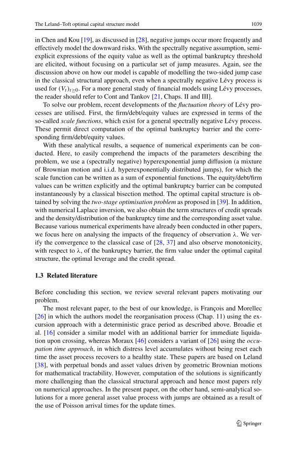
Fig. 3 The equity/debt/firm values as functions of V on (VB,∞) for VB = V ∗B
(solid) along withVB = V ∗
Bexp(ε) (dotted) for ε = −0.5,−0.4, . . . ,−0.1,0.1,0.2, . . . ,0.5. The values at V = VB are indi-
cated by circles for VB = V ∗B
, whereas those for VB < V ∗B
(resp. VB > V ∗B
) are indicated by up- (resp.down-) pointing triangles
6.2 Sensitivity with respect to λ of the equity value
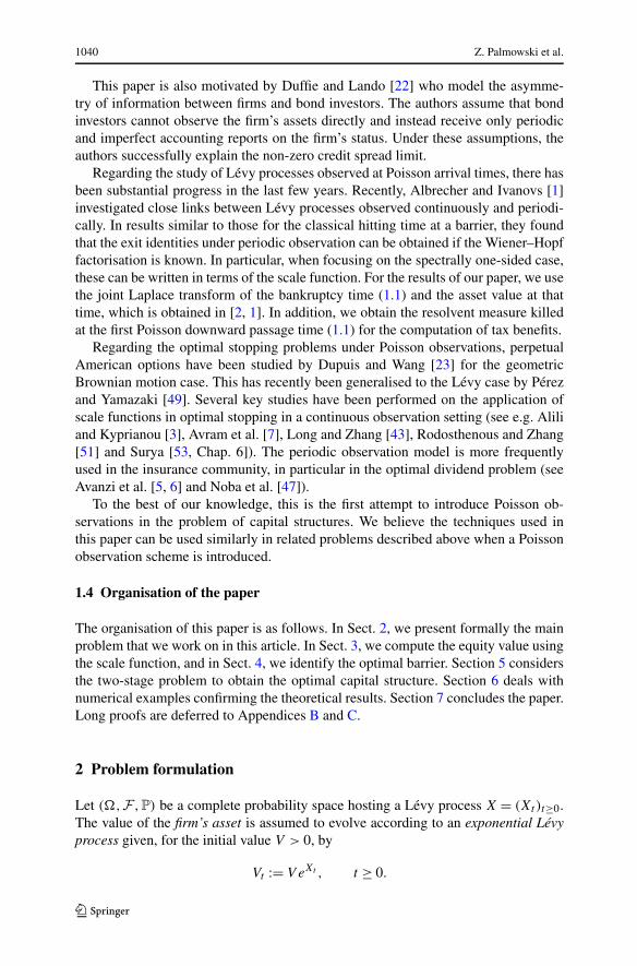
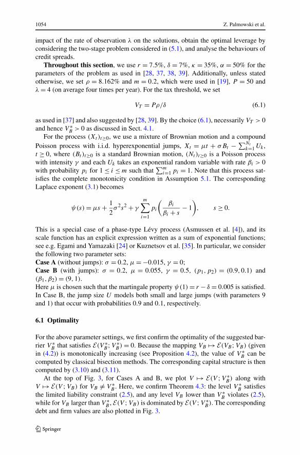
We now proceed to study the sensitivity of the optimal bankruptcy barrier and the eq-uity value with respect to the rate of observation λ. In the left plot of Fig. 4, we showthe equity value E( · ;V ∗
B) for various values of λ along with the classical (continuous-
1056 Z. Palmowski et al.
Fig. 4 (Top) The equity values E(V ;V ∗B
) (dotted) for λ = 1,2,4,6,12,52,365 along with the classi-
cal case E(V ; VB) (solid). The corresponding values at V = V ∗B
are indicated by circles. (Bottom) The
difference E(V ;V ∗B
) − E(V ; VB) for the same set of λ-values
observation) case as obtained in [28, 37]. We see that the optimal barrier V ∗B is de-
creasing in λ and converges to the optimal barrier, say VB , of the classical case. Thisconfirms Remark 4.9.
We also confirm the convergence of E(V ;V ∗B) to the classical case, say E(V ; VB),
for each starting value V . On the other hand, monotonicity of E(V ;V ∗B) with respect
to λ fails. When V is small, the equity value tends to be higher for small values ofλ, but it is not necessarily so for higher values of V . In order to investigate this, weshow in the bottom plots of Fig. 4 the difference E(V ;V ∗
B) − E(V ; VB). We observealso the differences between Cases A and B — in Case A, a lower value of λ clearlyachieves higher equity value when V is large whereas this is not clear in Case B.
6.3 Analysis of the bankruptcy time and the asset value at bankruptcy
While it was confirmed that the barrier level V ∗B is monotone in λ, it is not clear
how the distributions of (T −V ∗
B,VT −
V ∗B
) change in λ. Here, by taking advantage of the
joint Laplace transform (q, θ) → J (q,λ)( · ; θ) as in (3.7), we compute numerically
The Leland–Toft optimal capital structure model 1057
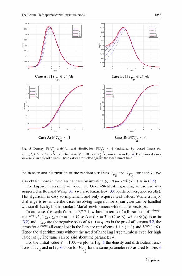
Fig. 5 Density P[T −V ∗
B∈ dt]/dt and distribution P[T −
V ∗B
≤ t] (indicated by dotted lines) for
λ = 1,2,4,6,12,52,365, the initial value V = 100 and V ∗B
determined as in Fig. 4. The classical casesare also shown by solid lines. These values are plotted against the logarithm of time
the density and distribution of the random variables T −V ∗
Band VT −
V ∗B
for each λ. We
also obtain those in the classical case by inverting (q, θ) → H(q)( · ; θ) as in (3.5).For Laplace inversion, we adopt the Gaver–Stehfest algorithm, whose use was
suggested in Kou and Wang [31] (see also Kuznetsov [33] for its convergence results).The algorithm is easy to implement and only requires real values. While a majorchallenge is to handle the cases involving large numbers, our case can be handledwithout difficulty in the standard Matlab environment with double precision.
In our case, the scale function W(q) is written in terms of a linear sum of e�(q)x
and e−ξi,qx , 1 ≤ i ≤ n (n = 1 in Case A and n = 3 in Case B), where �(q) is as in(3.2) and −ξi,q are the negative roots of ψ( · ) = q . As in the proof of Lemma 5.2, theterms for e�(q)x all cancel out in the Laplace transforms J (q,λ)( · ; θ) and H(q)( · ; θ).Hence the algorithm runs without the need of handling large numbers even for highvalues of q . The same can be said about the parameter θ .
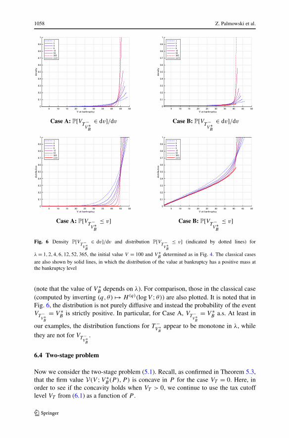
For the initial value V = 100, we plot in Fig. 5 the density and distribution func-tions of T −
V ∗B
and in Fig. 6 those for VT −V ∗B
for the same parameter sets as used for Fig. 4
1058 Z. Palmowski et al.
Fig. 6 Density P[VT −V ∗B
∈ dv]/dv and distribution P[VT −V ∗B
≤ v] (indicated by dotted lines) for
λ = 1,2,4,6,12,52,365, the initial value V = 100 and V ∗B
determined as in Fig. 4. The classical cases
are also shown by solid lines, in which the distribution of the value at bankruptcy has a positive mass atthe bankruptcy level
(note that the value of V ∗B depends on λ). For comparison, those in the classical case
(computed by inverting (q, θ) → H(q)(logV ; θ)) are also plotted. It is noted that inFig. 6, the distribution is not purely diffusive and instead the probability of the eventVT −
V ∗B
= V ∗B is strictly positive. In particular, for Case A, VT −
V ∗B
= V ∗B a.s. At least in
our examples, the distribution functions for T −V ∗
Bappear to be monotone in λ, while
they are not for VT −V ∗B
.
6.4 Two-stage problem
Now we consider the two-stage problem (5.1). Recall, as confirmed in Theorem 5.3,that the firm value V(V ;V ∗
B(P ),P ) is concave in P for the case VT = 0. Here, inorder to see if the concavity holds when VT > 0, we continue to use the tax cutofflevel VT from (6.1) as a function of P .

The Leland–Toft optimal capital structure model 1059
Fig. 7 The firm values (top) and debt values (bottom) as functions of the leverage P/V for the two-stage
problem for V = 100. The periodic cases with λ = 1,2,4,6,12,52,365 (dotted) are indicated by dotted
lines, and the classical case corresponds to the solid lines. The points at P ∗/V are indicated by circles
For our numerical results, we set V = 100 and obtain V ∗B for P running from 0 to
100 (leverage P/V running from 0 to 1). The corresponding firm and debt values arecomputed for each P and V ∗
B = V ∗B(P ), and shown in Fig. 7. For comparison, analo-
gous results on the classical case are also plotted. Here, the concavity with respect toP is confirmed in all considered cases.
Regarding the analysis with respect to λ, at least in these examples, we observethat the firm and debt values for each P are monotone in λ and converge to those inthe classical case. In addition, we see that the optimal face value P ∗ decreases in λ
and converges to that in the classical case.
6.5 The term structure of credit spreads
We now move on to the analysis of the credit spread. Let VB > 0 be a fixed bankruptcylevel. The credit spread is defined as the excess of the amount of coupon over the risk-free interest rate required to induce the investor to lend one dollar to the firm untilthe maturity time t . To be more precise, by finding the coupon rate ρ∗ that makesthe value of the debt d(V ;VB, t) defined in (2.2) of unit face value equal to one, thecredit spread ρ∗ − r is given after some rearrangement of (2.2) by
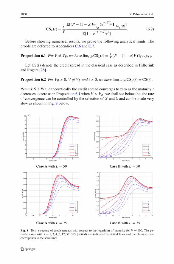
1060 Z. Palmowski et al.
CSλ(t) = r
P
E[(P − (1 − α)VTV
−B
)e−rT −
VB 1{T −VB
≤t}]
E[1 − e−r(t∧T −
VB)]
. (6.2)
Before showing numerical results, we prove the following analytical limits. Theproofs are deferred to Appendices C.6 and C.7.
Proposition 6.1 For V �= VB , we have limt↓0 CSλ(t) = λP
(P − (1 − α)V )1{V <VB }.
Let CS(t) denote the credit spread in the classical case as described in Hilberinkand Rogers [28].
Proposition 6.2 For VB > 0, V �= VB and t > 0, we have limλ→∞ CSλ(t) = CS(t).
Remark 6.3 While theoretically the credit spread converges to zero as the maturity t
decreases to zero as in Proposition 6.1 when V > VB , we shall see below that the rateof convergence can be controlled by the selection of X and λ and can be made veryslow as shown in Fig. 8 below.
Fig. 8 Term structure of credit spreads with respect to the logarithm of maturity for V = 100. The pe-riodic cases with λ = 1,2,4,6,12,52,365 (dotted) are indicated by dotted lines and the classical casecorresponds to the solid lines
The Leland–Toft optimal capital structure model 1061
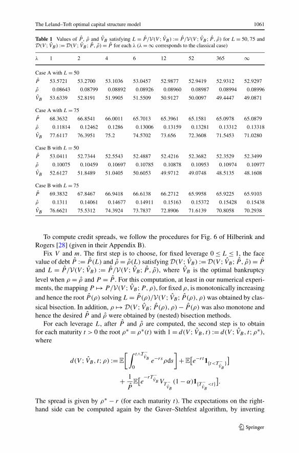
Table 1 Values of P , ρ and VB satisfying L = P /V(V ; VB) := P /V(V ; VB ; P , ρ) for L = 50,75 andD(V ; VB) :=D(V ; VB ; P , ρ) = P for each λ (λ = ∞ corresponds to the classical case)
λ 1 2 4 6 12 52 365 ∞
Case A with L = 50
P 53.5721 53.2700 53.1036 53.0457 52.9877 52.9419 52.9312 52.9297
ρ 0.08643 0.08799 0.08892 0.08926 0.08960 0.08987 0.08994 0.08996
VB 53.6339 52.8191 51.9905 51.5509 50.9127 50.0097 49.4447 49.0871
Case A with L = 75
P 68.3632 66.8541 66.0011 65.7013 65.3961 65.1581 65.0978 65.0879
ρ 0.11814 0.12462 0.1286 0.13006 0.13159 0.13281 0.13312 0.13318
VB 77.6117 76.3951 75.2 74.5702 73.656 72.3608 71.5453 71.0280
Case B with L = 50
P 53.0411 52.7344 52.5543 52.4887 52.4216 52.3682 52.3529 52.3499
ρ 0.10075 0.10459 0.10697 0.10785 0.10878 0.10953 0.10974 0.10977
VB 52.6127 51.8489 51.0405 50.6053 49.9712 49.0748 48.5135 48.1608
Case B with L = 75
P 69.3832 67.8467 66.9418 66.6138 66.2712 65.9958 65.9225 65.9103
ρ 0.1311 0.14061 0.14677 0.14911 0.15163 0.15372 0.15428 0.15438
VB 76.6621 75.5312 74.3924 73.7837 72.8906 71.6139 70.8058 70.2938
To compute credit spreads, we follow the procedures for Fig. 6 of Hilberink andRogers [28] (given in their Appendix B).
Fix V and m. The first step is to choose, for fixed leverage 0 ≤ L ≤ 1, the facevalue of debt P := P (L) and ρ = ρ(L) satisfying D(V ; VB) := D(V ; VB; P , ρ) = P
and L = P /V(V ; VB) := P /V(V ; VB; P , ρ), where VB is the optimal bankruptcy
level when ρ = ρ and P = P . For this computation, at least in our numerical experi-ments, the mapping P → P/V(V ; VB;P,ρ), for fixed ρ, is monotonically increasing
and hence the root P (ρ) solving L = P (ρ)/V(V ; VB; P (ρ), ρ) was obtained by clas-
sical bisection. In addition, ρ →D(V ; VB; P (ρ), ρ) − P (ρ) was also monotone andhence the desired P and ρ were obtained by (nested) bisection methods.
For each leverage L, after P and ρ are computed, the second step is to obtainfor each maturity t > 0 the root ρ∗ = ρ∗(t) with 1 = d(V ; VB, t) := d(V ; VB, t;ρ∗),where
d(V ; VB, t;ρ) := E
[∫ t∧T −VB
0e−rsρds
]+E
[e−rt1{t<T −
VB}]
+ 1
PE
[e−rT −
VB VT −VB
(1 − α)1{T −VB
<t}].
The spread is given by ρ∗ − r (for each maturity t). The expectations on the right-hand side can be computed again by the Gaver–Stehfest algorithm, by inverting
1062 Z. Palmowski et al.
q → J (q,λ)( · ; θ) as in (3.7) for θ = 0,1. Those for the classical case can be com-puted by inverting q → H(q)( · ; θ).
Here, we consider leverages L = 50,75 again for Cases A and B. In Table 1, thecomputed values of P , ρ and VB are listed for each λ = 1,2,4,6,12,52,365 alongwith those for the classical case. In Fig. 8, we plot the credit spread with respect tothe log maturity for each λ. For comparison, we also plot those in the classical case.The spread appears to be monotone in λ and converges to that in the classical casefor each maturity.
Regarding the credit spread limit, while the convergence to zero has been con-firmed in Proposition 6.1 for the periodic case, the rate of convergence depends sig-nificantly on the selection of λ and the underlying asset value process. In Case A(without negative jumps), the credit spread converges to zero quickly as the maturitydecreases. On the other hand, in Case B (where the credit spread does not convergeto zero as the maturity goes to zero in the continuous-observation case), the conver-gence to zero of the credit spread is very slow for large values of λ, as can be seenin Fig. 8. In view of these observations, with a selection of asset values with negativejumps and the observation rate λ, realistic short-maturity credit spread behaviourscan be achieved.
7 Concluding remarks
We have studied an extension of the Leland–Toft optimal capital structure modelwhere the information on the asset value is updated only at the jump times of anindependent Poisson process. In settings where the asset value follows an exponentialLévy process with negative jumps, we have obtained explicitly an optimal bankruptcystrategy and the corresponding equity/debt/firm values. These analytical results haveenabled us to efficiently conduct numerical experiments and further analysis of theimpact of the observation rate on the optimal leverages and credit spreads.
There are various venues for future research. First, it is a natural direction to con-sider the case in which the asset value process contains both positive and negativejumps. Because positive jumps do not have a direct influence on the model of the de-fault, similar results are expected, and for example the optimal barrier is likely to begiven by VB such that E(VB;VB) = 0. While the techniques using the scale functionemployed in this paper cannot be directly applied to two-sided jump cases, there areseveral potential alternative approaches. One approach would be to add phase-typeupward jumps to a spectrally negative Lévy process via fluid embedding and con-struct a Lévy process with two-sided jumps in terms of a Markov additive process.To do this, the phase-type jumps of the Lévy process can be substituted by linearstretches of unit slope. This procedure requires though adding a supplementary back-ground Markov chain; see e.g. Ivanovs [29, Sect. 2.7] for details. Another approachwould be to focus on a Lévy process with two-sided phase-type distributed jumpsand use them to approximate a general case. This may be possible by combining theresults of Asmussen et al. [4] and Albrecher et al. [2].
Second, it is important to consider the constant grace period case described in 1) ofSect. 1.1. As discussed, this paper’s results, featuring exponential grace periods, may

The Leland–Toft optimal capital structure model 1063
be used to approximate the constant case when the grace period is short. However, analternative approach is required when it is long. One potential approach would be touse Carr’s [17] randomisation method to approximate the constant period in terms ofan Erlang random variable, or the sum of i.i.d. exponential random variables. As inLeung et al. [40], a recursive algorithm may be constructed to compute the requiredfluctuation identities.
Acknowledgements The authors thank the anonymous referees and Co-Editor for careful reading ofthe paper and constructive comments and suggestions. They also thank Nan Chen, Sebastian Gryglewicz,and Tak-Yuen Wong for helpful comments and discussions. This paper was supported by the NationalScience Centre under the grant 2016/23/B/HS4/00566 (2017-2020) and by MEXT KAKENHI grant no.17K05377, 19H01791 and 20K03758. Part of the work was completed while Z. Palmowski was visitingKansai University and Kyoto University at the invitation of K. Yamazaki. Z. Palmowski is very gratefulfor the hospitality provided by Kazutoshi Yamazaki, Kouji Yano and Takashi Kumagai.
Publisher’s Note Springer Nature remains neutral with regard to jurisdictional claims in published mapsand institutional affiliations.
Open Access This article is licensed under a Creative Commons Attribution 4.0 International License,which permits use, sharing, adaptation, distribution and reproduction in any medium or format, as long asyou give appropriate credit to the original author(s) and the source, provide a link to the Creative Commonslicence, and indicate if changes were made. The images or other third party material in this article are in-cluded in the article’s Creative Commons licence, unless indicated otherwise in a credit line to the material.If material is not included in the article’s Creative Commons licence and your intended use is not permittedby statutory regulation or exceeds the permitted use, you will need to obtain permission directly from thecopyright holder. To view a copy of this licence, visit http://creativecommons.org/licenses/by/4.0/.
Appendix A: Relation between the bankruptcy model (1.1) andParisian ruin
Let G denote the set of starting points of the negative excursions of the shifted pro-cess (Vt − VB)t≥0 and consider a set of mutually independent exponential randomvariables {eg
λ : g ∈ G}, independent of (Vt )t≥0 as well. Let gt := sup{s ≤ t : Vs ≥ VB}be the last time before t the asset value was at or above VB (i.e., the starting point ofthe excursion). Then the Parisian ruin with exponential grace periods is defined as
inf{t > 0 : Vt < VB and t > gt + egt
λ }. (A.1)
The equivalence with (1.1) can be easily verified. In each negative excursion withstarting time g for the shifted process (Vt − VB)t≥0 between two Poisson observa-tion times, say Ti(g) and Ti(g)+1 for some i(g) ≥ 0, we consider the waiting timeTi(g)+1 − g until the next observation. Due to the lack of memory property of the ex-ponential distribution and the strong Markov property, these waiting times are equalin distribution to a set of mutually independent exponentially distributed random vari-ables. Consequently, (1.1) can be written as (A.1) with egt
λ replaced by these inde-pendent exponential random variables. In fact, it has been shown in Baurdoux et al.[10, Remark 1.1] that the joint distribution of the bankruptcy time (1.1) and the cor-responding position of X is the same as that of (A.1) and the corresponding positionof X (refer to Avram et al. [9] and Pardo et al. [48] for related literature).

1064 Z. Palmowski et al.
Table 2 The discounted assetvalues at bankruptcy
E[e−rτ−VB V
τ−VB
1{τ−VB
<∞}]when τ−
VBis the bankruptcy time
with constant or exponentialgrace periods with mean λ−1.The approximated values viaMonte Carlo simulation aredisplayed together with their95% confidence intervals. Weset r = 7.5% and use the Lévyprocesses given in Cases A(without jumps) and B (withnegative jumps) specified inSect. 6 so that (e−(r−δ)t Vt )t≥0
is a martingale for δ = 7%. Theinitial value of the process is100 and the bankruptcy level VB
is 40
λ Constant Exponential
Case A
1 4.710(4.674,4.747) 6.219(6.176,6.261)
2 5.795(5.753,5.838) 7.014(6.964,7.064)
4 6.717(6.674,6.760) 7.639(7.593,7.685)
6 7.125(7.070,7.179) 7.929(7.872,7.985)
12 7.727(7.668,7.785) 8.289(8.229,8.349)
52 8.543(8.492,8.595) 8.819(8.766,8.871)
365 8.886(8.824,8.947) 9.025(8.964,9.087)
Case B
1 6.238(6.192,6.283) 7.749(7.692,7.807)
2 7.434(7.388,7.480) 8.589(8.537,8.642)
4 8.472(8.417,8.528) 9.395(9.338,9.451)
6 8.825(8.770,8.880) 9.584(9.530,9.638)
12 9.436(9.376,9.496) 9.976(9.914,10.037)
52 10.184(10.125,10.242) 10.444(10.385,10.503)
365 10.726(10.673,10.778) 10.820(10.766,10.873)
It is worth investigating which impact the randomness of the grace period has onthe asset values at bankruptcy. To this end, we compare in Table 2 the expected dis-counted asset values at bankruptcy for the cases when the grace periods are constantor exponentially distributed (with the common mean λ−1). When λ is low, the ran-dom (exponential) case tends to overestimate the asset value, but as λ becomes larger(i.e., observation is more frequent), the differences become smaller. This implies thatwhen the observation is frequent, our model can approximate the constant grace pe-riod case reasonably well.
Appendix B: Proof of Proposition 3.2
For brevity, throughout this appendix, we use the notation
zT := z − logVT , z ∈R. (B.1)
We first obtain the q-resolvent measure of the spectrally negative Lévy process(Xt )t≥0 killed at the stopping time (3.6) in terms of the function H(q+λ)( · ; θ) as in(3.5) and
I (q,λ)(x, y) := W(q+λ)(x + y) − λ
∫ x
0W(q)(x − z)W(q+λ)(z + y)dz
− Z(q)(x;�(q + λ)
)W(q+λ)(y), q > 0, x, y ∈R.
The proof of the following result is given in Appendix D.
The Leland–Toft optimal capital structure model 1065
Theorem B.1 For any bounded measurable function h : R → R with compact sup-port,
Ex
[∫ T −z
0e−qth(Xt )dt
]=
∫R
h(y + z)R(q,λ)(x − z, y)dy, x, z ∈R,
where
R(q,λ)(x, y) := Z(q)(x;�(q + λ)
)�(q + λ) − �(q)
λH(q+λ)
( − y;�(q))
− I (q,λ)(x,−y). (B.2)
Using Theorem B.1, we show Proposition 3.2. The case VT = 0 is trivial, andhence we assume VT > 0 for the rest of this proof. By integrating the density inTheorem B.1 and using (B.1), we can write (3.9) as
(r,λ)(x, z) = Z(r)(x − z;�(r + λ)
)�(r + λ) − �(r)
λH(z) − I(x, z), (B.3)
where we define
H(z) :=∫ zT
−∞H(r+λ)
(y;�(r)
)dy, I(x, z) :=
∫ zT
−∞I (r,λ)(x − z, y)dy, (B.4)
which are shown to be finite immediately below. The rest of the proof of Proposi-tion 3.2 is devoted to the simplification of the integrals H and I .
Lemma B.2 We have W(r+λ)
(y) − λ∫ y
0 W(r)(y − z)W(r+λ)
(z)dz = W(r)
(y) for ally ∈ R.
Proof We have
∂
∂y
(W
(r+λ)(y) − λ
∫ y
0W(r)(y − z)W
(r+λ)(z)dz
)
= ∂
∂y
(W
(r+λ)(y) − λ
∫ y
0W(r)(z)W
(r+λ)(y − z)dz
)
= W(r+λ)(y) − λ
∫ y
0W(r)(z)W(r+λ)(y − z)dz = W(r)(y),
where the last equality holds by Loeffen et al. [42, identity (6)]. Integrating this and
because W(r+λ)
(0) = W(r)
(0) = 0, the proof is complete. �
Lemma B.3 We have for x, z ∈ R that
I(x, z) = W(r+λ)
(x − logVT )1{zT >0} + W(r)
(x − logVT )1{zT ≤0}
− λ
∫ x−z
0W(r)(x − z − u)W
(r+λ)(u + zT )du1{zT >0}
− Z(r)(x − z;�(r + λ)
)W
(r+λ)(zT ).

1066 Z. Palmowski et al.
Proof For zT > 0, we have∫ zT
0I (r,λ)(x − z, y)dy
=∫ zT
0W(r+λ)(x − z + y)dy − λ
∫ x−z
0W(r)(x − z − u)
∫ zT
0W(r+λ)(u + y)dydu
− Z(r)(x − z;�(r + λ)
)∫ zT
0W(r+λ)(y)dy
= W(r+λ)
(x − logVT ) − W(r+λ)
(x − z)
− λ
∫ x−z
0W(r)(x − z − u)
(W
(r+λ)(u + zT ) − W
(r+λ)(u)
)du
− Z(r)(x − z;�(r + λ)
)W
(r+λ)(zT )
= W(r+λ)
(x − logVT ) − W(r)
(x − z)
− λ
∫ x−z
0W(r)(x − z − u)W
(r+λ)(u + zT )du
− Z(r)(x − z;�(r + λ)
)W
(r+λ)(zT ),
where we used x − z + zT = x − logVT (see (B.1)) in the second equality andLemma B.2 in the last one. On the other hand, as in Pérez et al. [50, Remark 4.3(ii)],we have
I (r,λ)(x, y) = W(r)(x + y), y < 0, (B.5)
and therefore∫ 0∧zT
−∞I (r,λ)(x − z, y)dy =
∫ 0∧zT
−∞W(r)(x − z + y)dy = W
(r)(x − z + (0 ∧ zT )
).
Now the result is immediate by adding the two integrals and using (again see (B.1))
W(r)(
x − z + (0 ∧ zT )) =
{W
(r)(x − z) if zT > 0,
W(r)
(x − logVT ) if zT ≤ 0. �
We note that (B.3) together with Lemma B.3 implies that
(r,λ)(z, z) = �(r + λ) − �(r)
λ
∫ zT
−∞H(r+λ)
(y;�(r)
)dy, z ∈ R. (B.6)
Lemma B.4 For z ∈ R, we have
H(z) = 1
�(r)
(Z(r+λ)
(zT ;�(r)
) − λ�(r + λ)
�(r + λ) − �(r)W
(r+λ)(zT )
). (B.7)

The Leland–Toft optimal capital structure model 1067
Proof First, by (3.5), we have
H(r+λ)(y;�(r)
) = e�(r)y
(1 + λ
∫ y
0e−�(r)uW(r+λ)(u)du
)
− λ
�(r + λ) − �(r)W(r+λ)(y), y ∈R,
where in particular H(r+λ)(y;�(r)) = e�(r)y for y < 0. For zT > 0,
∫ zT
0e�(r)y
∫ y
0e−�(r)uW(r+λ)(u)dudy
=∫ zT
0
∫ zT
u
e�(r)ye−�(r)uW(r+λ)(u)dydu
=∫ zT
0
e�(r)zT − e�(r)u
�(r)e−�(r)uW(r+λ)(u)du
= 1
�(r)
(∫ zT
0e�(r)(zT −u)W(r+λ)(u)du − W
(r+λ)(zT )
),
and hence
∫ zT
0H(r+λ)
(y;�(r)
)dy
=∫ zT
0
(e�(r)y
(1 + λ
∫ y
0e−�(r)uW(r+λ)(u)du
)
− λ
�(r + λ) − �(r)W(r+λ)(y)
)dy
= 1
�(r)
(e�(r)zT − 1 + λ
∫ zT
0e�(r)(zT −u)W(r+λ)(u)du
− λ�(r + λ)
�(r + λ) − �(r)W
(r+λ)(zT )
)
= 1
�(r)
(Z(r+λ)
(zT ;�(r)
) − 1 − λ�(r + λ)
�(r + λ) − �(r)W
(r+λ)(zT )
).
On the other hand, for zT ∈R,
∫ zT ∧0
−∞H(r+λ)
(y;�(r)
)dy =
∫ zT ∧0
−∞e�(r)ydy = e�(r)(zT ∧0)/�(r).
By adding up the integrals, we obtain (B.7). �
Now applying Lemmas B.3 and B.4 in (B.3), we get Proposition 3.2. �

1068 Z. Palmowski et al.
Appendix C: Other proofs
C.1 Proof of Lemma 4.1
For the case VT > 0,
(r,λ)(z, z) = Ez
[∫ T −z
0e−rt1{Xt≥logVT }dt
]= E0
[∫ T −0
0e−rt1{Xt≥logVT −z}dt
]
is clearly nondecreasing in z, and by bounded convergence, limz↓−∞ (r,λ)(z, z) = 0.On the other hand, if VT = 0, then Proposition 3.2 and Remark 3.1, 1) yield
(r,λ)(z, z) = 1r(1 − J (r,λ)(0;0)) = 1
λ+r�(r+λ)�(r)
. �
C.2 Proof of Proposition 4.5
We start from several key introductory identities. Fix q > 0. Because
eθzZ(q)(x − z; θ) = eθx
(1 + (
q − ψ(θ))∫ x−z
0e−θuW(q)(u)du
),
we have for x �= z that
∂
∂z
(eθzZ(q)(x − z; θ)
) = −eθz(q − ψ(θ)
)W(q)(x − z),
∂
∂xZ(q)(x − z; θ) = ∂
∂x
(eθ(x−z)
(1 + (
q − ψ(θ)) ∫ x−z
0e−θuW(q)(u)du
))
= θZ(q)(x − z; θ) + (q − ψ(θ)
)W(q)(x − z).
In particular,
∂
∂xZ(q)
(x − z;�(r + λ)
) = �(r + λ)Z(q)(x − z;�(r + λ)
) − λW(q)(x − z).
(C.1)
Moreover, we have for x �= z that
∂
∂xJ (q,λ)(x − z; θ)
= λ
λ + q − ψ(θ)
∂
∂xZ(q)(x − z; θ)
− ψ(θ) − q
λ + q − ψ(θ)
�(q + λ) − �(q)
θ − �(q)
∂
∂xZ(q)
(x − z;�(q + λ)
)
= λ
λ + q − ψ(θ)θZ(q)(x − z; θ)
− ψ(θ) − q
λ + q − ψ(θ)
�(q + λ) − �(q)
θ − �(q)�(q + λ)Z(q)
(x − z;�(q + λ)
)
+ ψ(θ) − q
λ + q − ψ(θ)
�(q + λ) − θ
θ − �(q)λW(q)(x − z). (C.2)

The Leland–Toft optimal capital structure model 1069
By setting θ = 0, we obtain the following result.
Lemma C.1 We have for x �= z and q > 0 that
∂
∂zJ (q,λ)(x − z;0) = − ∂
∂xJ (q,λ)(x − z;0)
= q
λ + q
�(q + λ) − �(q)
�(q)�(q + λ)H(q)
(x − z;�(q + λ)
).
Noting that ∂∂z
(ezJ (q,λ)(x − z;1)) = ezJ (q,λ)(x − z;1)− ez ∂∂x
J (q,λ)(x − z;1) andusing (C.2) with θ = 1, we have the following result.
Lemma C.2 We have for x �= z and q > 0 that
∂
∂z
(ezJ (q,λ)(x − z;1)
)
= ψ(1) − q
λ + q − ψ(1)
�(q + λ) − �(q)
1 − �(q)
(�(q + λ) − 1
)ezH(q)
(x − z;�(q + λ)
).
We also need the following observation.
Lemma C.3 We have for zT �= 0 and x > z that
∂
∂z (r,λ)(x, z) = − (�(r + λ) − �(r))2
λH(r)
(x − z;�(r + λ)
)H(z).
Proof By differentiating the identity in Lemma B.3, for zT �= 0, by (C.1),
∂
∂zI(x, z) = −λ
∂
∂z
∫ x−z
0W(r)(w)W
(r+λ)(x − w − logVT )dw1{zT >0}
+ ∂
∂xZ(r)
(x − z;�(r + λ)
)W
(r+λ)(zT )
− Z(r)(x − z;�(r + λ)
) ∂
∂zW
(r+λ)(zT )
= λW(r)(x − z)W(r+λ)
(zT )
+(�(r + λ)Z(r)
(x − z;�(r + λ)
) − λW(r)(x − z))W
(r+λ)(zT )
− Z(r)(x − z;�(r + λ)
)W(r+λ)(zT )
= Z(r)(x − z;�(r + λ)
)(�(r + λ)W
(r+λ)(zT ) − W(r+λ)(zT )
). (C.3)
1070 Z. Palmowski et al.
By (3.5) and (C.1), we can write
∂
∂xZ(r)
(x − z;�(r + λ)
) = (�(r + λ) − �(r)
)H(r)
(x − z;�(r + λ)
)
+ �(r)Z(r)(x − z;�(r + λ)
). (C.4)
Using (B.4), we have for x > z and zT �= 0 that
∂
∂z
(Z(r)
(x − z;�(r + λ)
)H(z)
)= − ∂
∂xZ(r)
(x − z;�(r + λ)
)H(z) (C.5)
+ Z(r)(x − z;�(r + λ)
)H(r+λ)
(zT ;�(r)
).
By (B.7) and (C.4), this equals
− (�(r + λ) − �(r)
)H(r)
(x − z;�(r + λ)
)H(z)
+ Z(r)(x − z;�(r + λ)
)(H(r+λ)
(zT ;�(r)
) − �(r)H(z)).
Furthermore, by (B.7),
H(r+λ)(zT ;�(r)
) − �(r)H(z)
= H(r+λ)(zT ;�(r)
) − Z(r+λ)(zT ;�(r)
) + λ�(r + λ)
�(r + λ) − �(r)W
(r+λ)(zT )
= λ
�(r + λ) − �(r)
(�(r + λ)W
(r+λ)(zT ) − W(r+λ)(zT )
).
In sum, we have
∂
∂z
(Z(r)
(x − z;�(r + λ)
)H(z)
)
= −(�(r + λ) − �(r)
)H(r)
(x − z;�(r + λ)
)H(z)
+ λ
�(r + λ) − �(r)Z(r)
(x − z;�(r + λ)
)
× (�(r + λ)W
(r+λ)(zT ) − W(r+λ)(zT )
). (C.6)
By applying (C.3) and (C.6) in (B.3), the proof is complete. �
We now prove Proposition 4.5. Differentiating (3.11) and using Lemmas C.1–C.3gives
The Leland–Toft optimal capital structure model 1071
∂
∂VB
E(V ;VB)
= −V −1B
(α
ψ(1) − r
λ + r − ψ(1)
�(r + λ) − �(r)
1 − �(r)
(�(r + λ) − 1
)VB
+ Pκρ(�(r + λ) − �(r))2
λ
∫ log(VB/VT )
−∞H(r+λ)
(y;�(r)
)dy
)
× H(r)
(log
V
VB
;�(r + λ)
)
− V −1B
((1 − α)
ψ(1) − r − m
λ + r + m − ψ(1)
�(r + m + λ) − �(r + m)
1 − �(r + m)
× (�(r + m + λ) − 1
)VB
− Pρ + p
r + m
r + m
λ + r + m
�(r + m + λ) − �(r + m)
�(r + m)�(r + m + λ)
)
× H(r+m)
(log
V
VB
;�(r + m + λ)
),
which reduces to (4.5) after simplification using Remark 3.1, 1). �
C.3 Proof of Proposition 4.6
In view of the probabilistic expression (3.5), q → H(q)(x − z;�(q + λ)) is nonin-creasing for x, z ∈R, and hence
H(r)(x − z;�(r + λ))
H(r+m)(x − z;�(r + m + λ))≥ 1 for x, z ∈R.
On the other hand, because ψ is strictly convex and strictly increasing on [�(0),∞),its right inverse � is strictly concave, that is, �′(r + λ + x) − �′(r + x) < 0 forx,λ > 0. Therefore
�(r + λ) − �(r)
�(r + m + λ) − �(r + m)> 1 for λ > 0.
Combining these, we obtain
�(r + λ) − �(r)
�(r + m + λ) − �(r + m)
H(r)(x − z;�(r + λ))
H(r+m)(x − z;�(r + m + λ))> 1. (C.7)
By Remark 3.1, 2) and because (3.5) implies that H(r+λ) is nonnegative on R,we have
α(1 − J (r,λ)(0;1)
)ez + Pκρ
�(r + λ) − �(r)
λH(z) ≥ 0.
Combining this with (B.6), (C.7) and (4.2) gives

1072 Z. Palmowski et al.
L(logV, logVB)
= H(r)(logV − logVB;�(r + λ))
H(r+m)(logV − logVB;�(r + m + λ))
�(r + λ) − �(r)
�(r + m + λ) − �(r + m)
×(
α(1 − J (r,λ)(0;1)
)VB
+ Pκρ�(r + λ) − �(r)
λ
∫ logVB−logVT
−∞H(r+λ)
(y;�(r)
)dy
)
+ (1 − α)(1 − J (r+m,λ)(0;1)
)VB − Pρ + p
r + m
(1 − J (r+m,λ)(0;0)
)> α
(1 − J (r,λ)(0;1)
)VB + Pκρ (r,λ)(logVB, logVB)
+ (1 − α)(1 − J (r+m,λ)(0;1)
)VB − Pρ + p
r + m
(1 − J (r+m,λ)(0;0)
)= E(VB;VB).
In addition, because VB ≥ V ∗B , the monotonicity in Proposition 4.2 implies that
E(VB;VB) ≥ 0. Note when V ∗B = 0 that E(VB;VB) ≥ 0 for all VB > 0 by Propo-
sition 4.2.Now by Proposition 4.5 and recalling that H(r+m) is positive,
∂
∂VB
E(V ;VB)
< −(�(r + m + λ) − �(r + m)
)H(r+m)
(log
V
VB
;�(r + m + λ)
)E(VB;VB)
VB
≤ 0. �
C.4 Proof of Proposition 4.7
Using Lemma B.3 together with (C.1) and (C.3), for x �= logVT and z ∈ R such thatzT �= 0, we have
∂
∂xI(x, z) = W(r+λ)(x − logVT )1{zT >0} + W(r)(x − logVT )1{zT <0}
− ∂
∂xλ
∫ x−z
0W(r)(w)W
(r+λ)(x − z − w + zT )dw1{zT >0}
− ∂
∂xZ(r)
(x − z;�(r + λ)
)W
(r+λ)(zT )
= W(r+λ)(x − logVT )1{zT >0} + W(r)(x − logVT )1{zT <0}
− λ
∫ x−z
0W(r)(w)W(r+λ)(x − z − w + zT )dw1{zT >0}
− λW(r)(x − z)W(r+λ)
(zT )
−(�(r + λ)Z(r)
(x − z;�(r + λ)
) − λW(r)(x − z))W
(r+λ)(zT )
= I (r,λ)(x − z, zT ) − ∂
∂zI(x, z), (C.8)

The Leland–Toft optimal capital structure model 1073
where we used (B.5) for the case zT < 0. Hence using (C.5) and (C.8) in (B.3), andby (B.2),
∂
∂x (r,λ)(x, z) = − ∂
∂z (r,λ)(x, z) + R(r,λ)(x − z,−zT ). (C.9)
Now we write (3.11) as
E(V ;VB) = A(logV, logVB) + Pκρ (r,λ)(logV, logVB), (C.10)
where
A(x, z) := ex − αezJ (r,λ)(x − z;1) − Pρ + p
r + m
(1 − J (r+m,λ)(x − z;0)
)− (1 − α) ezJ (r+m,λ)(x − z;1).
Differentiating this with respect to x and z, we get
∂
∂xA(x, z) = ex − αez ∂
∂xJ (r,λ)(x − z;1) + Pρ + p
r + m
∂
∂xJ (r+m,λ)(x − z;0)
− (1 − α) ez ∂
∂xJ (r+m,λ)(x − z;1),
∂
∂zA(x, z) = −αezJ (r,λ)(x − z;1) + αez ∂
∂xJ (r,λ)(x − z;1)
− Pρ + p
r + m
∂
∂xJ (r+m,λ)(x − z;0) − (1 − α) ezJ (r+m,λ)(x − z;1)
+ (1 − α) ez ∂
∂xJ (r+m,λ)(x − z;1),
and hence
∂
∂xA(x, z) = ex − ∂
∂zA(x, z) − αezJ (r,λ)(x − z;1)
− (1 − α)ezJ (r+m,λ)(x − z;1). (C.11)
Finally, using (C.9) and (C.11) in (C.10), we obtain
∂
∂VE(V ;VB) = 1
V
∂
∂x
(A(x, logVB) + Pκρ (r,λ)(x, logVB)
)∣∣∣∣x=logV
= 1
V
(V − ∂
∂zA(logV, z)
∣∣∣∣z=logVB
− αVBJ (r,λ)(
logV
VB
;1)
− (1 − α)VBJ (r+m,λ)(
logV
VB
;1)
− Pκρ∂
∂z (r,λ)(logV, z)
∣∣∣∣z=logVB
+ PκρR(r,λ)(
logV
VB
, logVT
VB
)),
1074 Z. Palmowski et al.
which reduces to the desired expression by noting that (C.10) gives
∂
∂VB
E(V ;VB) = 1
VB
(∂
∂zA(logV, z)
∣∣∣∣z=logVB
+ Pκρ∂
∂z (r,λ)(logV, z)
∣∣∣∣z=logVB
).
�
C.5 Proof of Lemma 4.10
First we note by Bertoin [11, Theorem VII.4] that for q ≥ 0,
limλ→∞
�(λ + r + m)
�(λ + q)= 1. (C.12)
On the other hand, (B.6) implies for VB > 0 that
λ
�(r + λ) − �(r) (r,λ)(logVB, logVB)
=⎧⎨⎩
1�(r)
(VB
VT)�(r) if VB/VT < 1,
1�(r)
+ ∫ log(VB/VT )
0 H(r+λ)(y;�(r))dy if VB/VT ≥ 1,
where we used H(r+λ)(y;�(r)) = exp(�(r)y) for y ≤ 0. In addition, by the prob-abilistic expression of H(r+λ) given in (3.5) and using dominated convergence,we have
limλ→∞
∫ log(VB/VT )
0H(r+λ)
(y;�(r)
)dy = 0.
This together with (C.12) gives
limλ→∞
λ + r + m
�(λ + r + m) (r,λ)(logVB, logVB) = 1
�(r)
((VB
VT
)�(r) ∧ 1
).
From Remark 3.1, 1) and (C.12), we can conclude that for q ≥ 0,
λ + r + m
�(λ + r + m)
(1 − J (q,λ)(0;1)
)
= λ + r + m
�(λ + r + m)
ψ(1) − q
λ + q − ψ(1)
�(q + λ) − 1
1 − �(q)
λ↑∞−−−→ ψ(1) − q
1 − �(q).
Combining these and (4.2), we obtain (4.8). �
C.6 Proof of Proposition 6.1
Fix t > 0. Let us define the event
E := {Nλt = 1} = {T λ
1 ≤ t, T λ2 > t} = {T λ
1 ≤ t, S > t − T λ1 },
The Leland–Toft optimal capital structure model 1075
where S := T λ2 − T λ
1 has an exponential distribution with parameter λ. Note that
E ∩ {T −VB
< t} = {T λ1 ≤ t, VT λ
1< VB, S > t − T λ
1 }. (C.13)
We start by analysing the numerator of (6.2). We decompose it as
f (t) := E[(
P − (1 − α)VT −VB
)e−rT −
VB 1{T −VB
≤t}] = f1(t) + f2(t),
where
f1(t) := E[(
P − (1 − α)VT −VB
)e−rT −
VB 1{T −VB
≤t} 1E
],
f2(t) := E[(
P − (1 − α)VT −VB
)e−rT −
VB 1{T −VB
≤t} 1Ec
].
Here, by (C.13) and because S is an independent exponential random variable withparameter λ,
f1(t) = E[(
P − (1 − α)VT λ1
)e−rT λ
1 1{T λ1 ≤t,V
T λ1
<VB, S>t−T λ1 }
]
= E[(
P − (1 − α)VT λ1
)e−rT λ
1 e−λ(t−T λ1 )1{T λ
1 ≤t,VT λ
1<VB }
]
= E
[∫ t
0λe−λs
(P − (1 − α)Vs
)e−rse−λ(t−s)1{Vs<VB }ds
]
= λe−λtE
[∫ t
0
(P − (1 − α)Vs
)e−rs1{Vs<VB }ds
],
and |f2(t)| ≤ (|P | + (1 − α)VB)P[Nλt ≥ 2] = o(t) as t ↓ 0. Summing f1(t) and
f2(t),
f (t) = λe−λtE
[∫ t
0
(P − (1 − α)Vs
)e−rs1{Vs<VB }ds
]+ o(t). (C.14)
On the other hand, we transform the denominator of (6.2) as
g(t) := E[1 − e
−r(t∧T −VB
)] = 1 − e−rt + g1(t) + g2(t),
where
g1(t) := E[(e−rt − e
−rT −VB )1{T −
VB≤t}1E
],
g2(t) := E[(e−rt − e
−rT −VB )1{T −
VB≤t}1Ec
].
Similarly to the computation for f1(t) and f2(t), by (C.13),

1076 Z. Palmowski et al.
g1(t) = E[(e−rt − e−rT λ
1 )1{T λ1 ≤t,V
T λ1
<VB,S>t−T λ1 }
]
= E[e−λ(t−T λ
1 )(e−rt − e−rT λ1 )1{T λ
1 ≤t,VT λ
1<VB }
]
= λe−λtE
[∫ t
0(e−rt − e−rs)1{Vs<VB }ds
],
and g2(t) ≤ P[Nλt ≥ 2] = o(t). Hence putting all the pieces together, we get that
g(t) = 1 − e−rt + λe−λtE
[∫ t
0(e−rt − e−rs)1{Vs<VB }ds
]+ o(t). (C.15)
Now from (C.14), (C.15) and the mean value theorem,
limt→0
f (t)
t= lim
t→0
1
t
(λe−λt
E
[∫ t
0
(P − (1 − α)Vs
)e−rs1{Vs<VB }ds
]+ o(t)
)
= λ(P − (1 − α)V
)1{V <VB },
limt→0
g(t)
t= lim
t→0
1
t
(1 − e−rt + λe−λt
E
[∫ t
0(e−rt − e−rs)1{Vs<VB }ds
]+ o(t)
)
= r.
By dividing the first by the second limit, we have the claim. �
C.7 Proof of Proposition 6.2
By (3.5) and (3.7), we can write for any θ ≥ 0 and q ≥ 0 that
J (q,λ)(y; θ)
= λ
λ + q − ψ(θ)
(H(q)(y; θ) − ψ(θ) − q
λ
�(q + λ) − �(q)
θ − �(q)H(q)
(y;�(q + λ)
)).
For y �= 0, we now note the following:1) For the cases (i) y < 0 or (ii) y > 0 and X does not have a diffusion component,
we have that H(q)(y;�(q + λ))λ↑∞−−−→ 0 (because the process does not creep down-
ward as in Kyprianou [36, Exercise 7.6]) and �(q+λ)−�(q)λ
is bounded for λ ≥ δ > 0(which can be verified by the convexity of ψ ).
2) For the case where y > 0 and X has a diffusion component,
H(q)(y;�(q + λ)
) λ↑∞−−−→ Ey
[e−qτ−
0 1{Xτ−0
=0,τ−0 <∞}
]
and �(q+λ)−�(q)λ
λ↑∞−−−→ 0 (because ψ(θ) ∼ 12σ 2θ2 as θ → ∞, where σ is the diffu-
sion coefficient of X). Hence the previous arguments imply that for y �= 0,
limλ→∞J (q,λ)(y; θ) = H(q)(y; θ), θ ≥ 0.
The Leland–Toft optimal capital structure model 1077
Given that J (q,λ)(y; θ) is the Laplace transform of the random vector (T −0 (λ),X
T −0 (λ)
)
(where we put (λ) to spell out the dependence on λ), Lévy’s continuity theoremimplies that (T −
0 (λ),XT −
0(λ)) converges in distribution to (τ−
0 ,Xτ−0). Hence using
Skorohod’s representation theorem (see Billingsley [13, Theorem 6.7]) as well asdominated convergence, we obtain for V �= VB that
limλ→∞ CSλ(t) = r
Plim
λ→∞Elog(V/VB)[(P − (1 − α)VBe
XT
−0 (λ) )e−rT −
0 (λ)1{T −0 (λ)≤t}]
Elog(V/VB)[1 − e−r(t∧T −0 (λ))]
= r
P
Elog(V/VB)[(P − (1 − α)VBeX
τ−0 )e−rτ−
0 1{τ−0 ≤t}]
Elog(V/VB)[1 − e−r(t∧τ−0 )]
= CS(t).�
Appendix D: Proof of Theorem B.1
From Kuznetsov et al. [35, Theorem 2.7], for any Borel set A in [0,∞), in R and in(−∞,0], respectively, we have
Ex
[∫ τ−0
0e−qt1{Xt∈A}dt
]
=∫
A
(e−�(q)yW(q)(x) − W(q)(x − y)
)dy, x ≥ 0, (D.1)
Ex
[∫ ∞
0e−(q+λ)t1{Xt∈A}dt
]
=∫
A
(e�(q+λ)(x−y)
ψ ′(�(q + λ))− W(q+λ)(x − y)
)dy, x ∈ R, (D.2)
Ex
[∫ τ+0
0e−(q+λ)t1{Xt∈A}dt
]
=∫
A
(e�(q+λ)xW(q+λ)(−y) − W(q+λ)(x − y)
)dy, x ≤ 0, (D.3)
where τ−0 is defined in (3.4) and τ+
0 := inf{t ≥ 0 : Xt > 0}.We prove the result for z = 0 and compute
g(x) := Ex
[∫ T −0
0e−qth(Xt )dt
], x ∈ R.
The general case follows because the spatial homogeneity of the Lévy process implies
that Ex[∫ T −
z
0 e−qth(Xt )dt] = Ex−z[∫ T −
00 e−qth(Xt + z)dt] for x, z ∈R.
For x ∈R, by the strong Markov property,
g(x) = Ex
[∫ τ−0
0e−qth(Xt )dt
]+Ex
[e−qτ−
0 g(Xτ−0)1{τ−
0 <∞}]. (D.4)

1078 Z. Palmowski et al.
In particular, for x < 0, again by the strong Markov property,
g(x) = A(x)g(0) + B(x),
where for x ≤ 0,
A(x) := Ex
[e−qτ+
0 1{τ+0 <T λ
1 }] = Ex
[e−(q+λ)τ+
0] = e�(q+λ)x,
B(x) := Ex
[∫ τ+0
0e−qt1{t<T λ
1 }h(Xt )dt
]
=∫ 0
−∞h(y)
(e�(q+λ)xW(q+λ)(−y) − W(q+λ)(x − y)
)dy.
Here the first equality for A(x) holds by the fact that T λ1 is an independent exponential
random variable with parameter λ and Kyprianou [36, Theorem 3.12]. The equalityfor B(x) is a consequence of (D.3).
Now by (3.5),
Ex
[e−qτ−
0 A(Xτ−0)1{τ−
0 <∞}] = H(q)
(x;�(q + λ)
), x ∈R,
for the function H(q) defined in (3.5). In addition, by Pérez et al. [50, proof of Theo-rem 4.1], we have
Ex
[e−qτ−
0 B(Xτ−0)1{τ−
0 <∞}] = W(q)(x)
∫ 0
−∞h(y)H(q+λ)
( − y;�(q))dy
−∫ 0
−∞h(y)I (q,λ)(x,−y)dy.
Substituting these in (D.4) and then applying (D.1) and [50, Remark 4.3], we obtainfor all x ∈ R that
g(x) = g(0)H (q)(x;�(q + λ)
) + W(q)(x)
∫ ∞
−∞h(y)H(q+λ)
( − y;�(q))dy
−∫ ∞
−∞h(y)I (q,λ)(x,−y)dy. (D.5)
On the other hand, by the strong Markov property, we can also write
g(0) = E0
[E0
[∫ T λ1
0e−qth(Xt )dt
+ 1{XT λ
1>0}
∫ T −0
T λ1
e−qth(Xt )dt
∣∣∣T λ1 , (Xu)0≤u≤T λ
1
]]
= γ1 + γ2, (D.6)
The Leland–Toft optimal capital structure model 1079
where
γ1 := E0
[∫ T λ1
0e−qth(Xt )dt
], γ2 := E0
[e−qT λ
1 g(XT λ1)1{X
T λ1
>0}].
We compute γ1 and γ2 below. First observe that
γ1 = E0
[∫ ∞
01{t<T λ
1 }e−qth(Xt )dt
]= E0
[∫ ∞
0e−(q+λ)th(Xt )dt
].
For γ2, by (D.2), we can write
γ2 = λE0
[∫ ∞
0e−(q+λ)sg(Xs)1{Xs>0}ds
]
= λ
ψ ′(�(q + λ))
∫ ∞
0e−�(q+λ)yg(y)dy, (D.7)
which we compute by using the expression of g in (D.5). First, by [50, identity (A.8)],we have
∫ ∞
0e−�(q+λ)yZ(q)
(y;�(q + λ)
)dy = ψ ′(�(q + λ))
λ,
while (3.3) gives∫ ∞
0 e−�(q+λ)yW(q)(y)dy = λ−1, and therefore
∫ ∞
0e−�(q+λ)yH (q)
(y;�(q + λ)
)dy = ψ ′(�(q + λ))
λ− 1
�(q + λ) − �(q).
Again by [50, proof of Theorem 4.1], we have
∫ ∞
0e−�(q+λ)y
∫ ∞
−∞h(z)I (q,λ)(y,−z)dzdy
= ψ ′(�(q + λ))
λE0
[∫ ∞
0e−(q+λ)th(Xt )dt
].
Substituting these in (D.7) and with the help of (D.5),
γ2 = g(0)λ
ψ ′(�(q + λ))
(ψ ′(�(q + λ))
λ− 1
�(q + λ) − �(q)
)
−E0
[∫ ∞
0e−(q+λ)th(Xt )dt
]
+ 1
ψ ′(�(q + λ))
∫ ∞
−∞h(y)H(q+λ)
( − y;�(q))dy.
Now substituting the computed values of γ1 and γ2 in (D.6), we obtain

1080 Z. Palmowski et al.
g(0) = g(0) − λ
�(q + λ) − �(q)
g(0)
ψ ′(�(q + λ))
+ 1
ψ ′(�(q + λ))
∫ ∞
−∞h(y)H(q+λ)
( − y;�(q))dy,
and hence solving for g(0), we obtain
g(0) = �(q + λ) − �(q)
λ
∫ ∞
−∞h(y)H(q+λ)
( − y;�(q))dy.
Substituting this back in (D.5), we have
g(x) = Z(q)(x;�(q + λ)
)�(q + λ) − �(q)
λ
∫ ∞
−∞h(y)H(q+λ)
( − y;�(q))dy
−∫ ∞
−∞h(y)I (q,λ)(x,−y)dy.
Hence the resolvent density is given by (B.2), as claimed. �
References
1. Albrecher, H., Ivanovs, J.: Strikingly simple identities relating exit problems for Lévy processes undercontinuous and Poisson observations. Stoch. Process. Appl. 127, 643–656 (2017)
2. Albrecher, H., Ivanovs, J., Zhou, X.: Exit identities for Lévy processes observed at Poisson arrivaltimes. Bernoulli 22, 1364–1382 (2016)
3. Alili, L., Kyprianou, A.E.: Some remarks on first passage of Lévy processes, the American put andpasting principles. Ann. Appl. Probab. 15, 2062–2080 (2005)
4. Asmussen, S., Avram, F., Pistorius, M.R.: Russian and American put options under exponential phase-type Lévy models. Stoch. Process. Appl. 109, 79–111 (2004)
5. Avanzi, B., Cheung, E.C., Wong, B., Woo, J.K.: On a periodic dividend barrier strategy in the dualmodel with continuous monitoring of solvency. Insur. Math. Econ. 52, 98–113 (2013)
6. Avanzi, B., Tu, V., Wong, B.: On optimal periodic dividend strategies in the dual model with diffusion.Insur. Math. Econ. 55, 210–224 (2014)
7. Avram, F., Kyprianou, A.E., Pistorius, M.R.: Exit problems for spectrally negative Lévy processesand applications to (Canadized) Russian options. Ann. Appl. Probab. 14, 215–238 (2004)
8. Avram, F., Palmowski, Z., Pistorius, M.: On the optimal dividend problem for a spectrally negativeLévy process. Ann. Appl. Probab. 17, 156–180 (2007)
9. Avram, F., Pérez, J.L., Yamazaki, K.: Spectrally negative Lévy processes with Parisian reflectionbelow and classical reflection above. Stoch. Process. Appl. 128, 255–290 (2018)
10. Baurdoux, E.J., Pardo, J.C., Pérez, J.L., Renaud, J.F.: Gerber–Shiu distribution at Parisian ruin forLévy insurance risk processes. J. Appl. Probab. 53, 572–584 (2016)
11. Bertoin, J.: Lévy Processes. Cambridge University Press, Cambridge (1996)12. Bielecki, T.R., Rutkowski, M.: Credit Risk: Modeling, Valuation and Hedging. Springer, Berlin
(2013)13. Billingsley, P.: Convergence of Probability Measures, 2nd edn. Wiley, New York (1999)14. Black, F., Cox, J.: Valuing corporate securities: some effects of bond indenture provisions. J. Finance
31, 351–367 (1976)15. Brealey, R.A., Myers, S.C.: Principles of Corporate Finance. McGraw-Hill, New York (2001)16. Broadie, M., Chernov, M., Sundaresan, S.: Optimal debt and equity values in the presence of Chap. 7
and Chap. 11. J. Finance 62, 1341–1377 (2007)17. Carr, P.: Randomization and the American put. Rev. Financ. Stud. 11, 597–626 (1998)
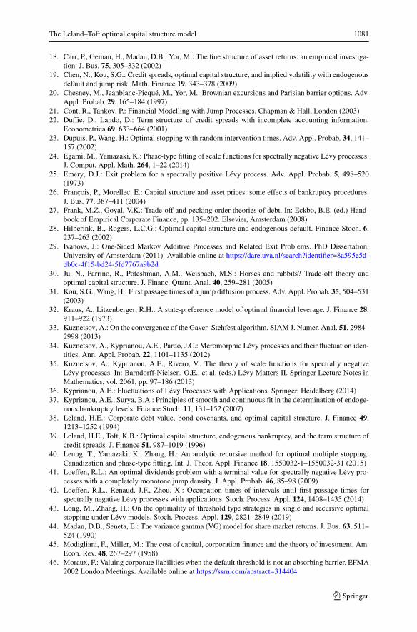
The Leland–Toft optimal capital structure model 1081
18. Carr, P., Geman, H., Madan, D.B., Yor, M.: The fine structure of asset returns: an empirical investiga-tion. J. Bus. 75, 305–332 (2002)
19. Chen, N., Kou, S.G.: Credit spreads, optimal capital structure, and implied volatility with endogenousdefault and jump risk. Math. Finance 19, 343–378 (2009)
20. Chesney, M., Jeanblanc-Picqué, M., Yor, M.: Brownian excursions and Parisian barrier options. Adv.Appl. Probab. 29, 165–184 (1997)
21. Cont, R., Tankov, P.: Financial Modelling with Jump Processes. Chapman & Hall, London (2003)22. Duffie, D., Lando, D.: Term structure of credit spreads with incomplete accounting information.
Econometrica 69, 633–664 (2001)23. Dupuis, P., Wang, H.: Optimal stopping with random intervention times. Adv. Appl. Probab. 34, 141–
157 (2002)24. Egami, M., Yamazaki, K.: Phase-type fitting of scale functions for spectrally negative Lévy processes.
J. Comput. Appl. Math. 264, 1–22 (2014)25. Emery, D.J.: Exit problem for a spectrally positive Lévy process. Adv. Appl. Probab. 5, 498–520
(1973)26. François, P., Morellec, E.: Capital structure and asset prices: some effects of bankruptcy procedures.
J. Bus. 77, 387–411 (2004)27. Frank, M.Z., Goyal, V.K.: Trade-off and pecking order theories of debt. In: Eckbo, B.E. (ed.) Hand-
book of Empirical Corporate Finance, pp. 135–202. Elsevier, Amsterdam (2008)28. Hilberink, B., Rogers, L.C.G.: Optimal capital structure and endogenous default. Finance Stoch. 6,
237–263 (2002)29. Ivanovs, J.: One-Sided Markov Additive Processes and Related Exit Problems. PhD Dissertation,
University of Amsterdam (2011). Available online at https://dare.uva.nl/search?identifier=8a595e5d-db0c-4f15-bd24-5fd7767a9b2d
30. Ju, N., Parrino, R., Poteshman, A.M., Weisbach, M.S.: Horses and rabbits? Trade-off theory andoptimal capital structure. J. Financ. Quant. Anal. 40, 259–281 (2005)
31. Kou, S.G., Wang, H.: First passage times of a jump diffusion process. Adv. Appl. Probab. 35, 504–531(2003)
32. Kraus, A., Litzenberger, R.H.: A state-preference model of optimal financial leverage. J. Finance 28,911–922 (1973)
33. Kuznetsov, A.: On the convergence of the Gaver–Stehfest algorithm. SIAM J. Numer. Anal. 51, 2984–2998 (2013)
34. Kuznetsov, A., Kyprianou, A.E., Pardo, J.C.: Meromorphic Lévy processes and their fluctuation iden-tities. Ann. Appl. Probab. 22, 1101–1135 (2012)
35. Kuznetsov, A., Kyprianou, A.E., Rivero, V.: The theory of scale functions for spectrally negativeLévy processes. In: Barndorff-Nielsen, O.E., et al. (eds.) Lévy Matters II. Springer Lecture Notes inMathematics, vol. 2061, pp. 97–186 (2013)
36. Kyprianou, A.E.: Fluctuations of Lévy Processes with Applications. Springer, Heidelberg (2014)37. Kyprianou, A.E., Surya, B.A.: Principles of smooth and continuous fit in the determination of endoge-
nous bankruptcy levels. Finance Stoch. 11, 131–152 (2007)38. Leland, H.E.: Corporate debt value, bond covenants, and optimal capital structure. J. Finance 49,
1213–1252 (1994)39. Leland, H.E., Toft, K.B.: Optimal capital structure, endogenous bankruptcy, and the term structure of
credit spreads. J. Finance 51, 987–1019 (1996)40. Leung, T., Yamazaki, K., Zhang, H.: An analytic recursive method for optimal multiple stopping:
Canadization and phase-type fitting. Int. J. Theor. Appl. Finance 18, 1550032-1–1550032-31 (2015)41. Loeffen, R.L.: An optimal dividends problem with a terminal value for spectrally negative Lévy pro-
cesses with a completely monotone jump density. J. Appl. Probab. 46, 85–98 (2009)42. Loeffen, R.L., Renaud, J.F., Zhou, X.: Occupation times of intervals until first passage times for
spectrally negative Lévy processes with applications. Stoch. Process. Appl. 124, 1408–1435 (2014)43. Long, M., Zhang, H.: On the optimality of threshold type strategies in single and recursive optimal
stopping under Lévy models. Stoch. Process. Appl. 129, 2821–2849 (2019)44. Madan, D.B., Seneta, E.: The variance gamma (VG) model for share market returns. J. Bus. 63, 511–
524 (1990)45. Modigliani, F., Miller, M.: The cost of capital, corporation finance and the theory of investment. Am.
Econ. Rev. 48, 267–297 (1958)46. Moraux, F.: Valuing corporate liabilities when the default threshold is not an absorbing barrier. EFMA
2002 London Meetings. Available online at https://ssrn.com/abstract=314404

1082 Z. Palmowski et al.
47. Noba, K., Pérez, J.L., Yamazaki, K., Yano, K.: On optimal periodic dividend strategies for Lévy riskprocesses. Insur. Math. Econ. 80, 29–44 (2018)
48. Pardo, J.C., Pérez, J.L., Rivero, V.M.: The excursion measure away from zero for spectrally negativeLévy processes. Ann. Inst. Henri Poincaré Probab. Stat. 54, 75–99 (2018)
49. Pérez, J.L., Yamazaki, K.: American options under periodic exercise opportunities. Stat. Probab. Lett.135, 92–101 (2018)
50. Pérez, J.L., Yamazaki, K., Bensoussan, A.: Optimal periodic replenishment policies for spectrallypositive Lévy processes. Preprint (2018). Available online at https://arxiv.org/abs/1806.09216
51. Rodosthenous, N., Zhang, H.: Beating the omega clock: an optimal stopping problem with randomtime-horizon under spectrally negative Lévy models. Ann. Appl. Probab. 28, 2105–2140 (2018)
52. Sims, C.A.: Implications of rational inattention. J. Monet. Econ. 50, 665–690 (2003)53. Surya, B.A.: Optimal Stopping of Lévy Processes and Pasting Principles. PhD dissertation, Univer-
sity of Utrecht (2007). Available online at https://dspace.library.uu.nl/bitstream/handle/1874/19086/full.pdf
54. Surya, B.A., Yamazaki, K.: Optimal capital structure with scale effects under spectrally negative Lévymodels. Int. J. Theor. Appl. Finance 17, 1450013-1–1450013-31 (2014)
55. Takács, L.: Combinatorial Methods in the Theory of Stochastic Processes. Wiley, New York (1966)56. Zolotarev, V.M.: The first passage time of a level and the behavior at infinity for a class of processes
with independent increments. Theory Probab. Appl. 9, 653–664 (1964)