LECTURE 27 The Lessons and Tools of Economics

May 3, 2016

Economics 2 Christina Romer Spring 2016 David Romer

Announcements

• Suggested answers for Problem Set 6 are available on the course website.

Final Exam Logistics

• Friday, May 13th, 7–10 p.m.

• In Wheeler Auditorium

• Please sit every other seat.

• You will be getting out late, so make plans now for getting home safely.

Final Exam Format and Content

• Roughly the length of two midterms.

• Cumulative, but with one section specifically on material since the second midterm.

• Mixture of T/F/U questions, problems, and multiple choice questions.

Some Advice on Taking the Final Exam

• Read questions carefully.

• Figure out what tool is appropriate.

• Watch your time.

• Think of trying to convince the person grading the exam that you understand the material.

Some Advice on Studying

• Focus on the posted slides and your lecture notes.

• Also the suggested answers to the problem sets.

• Study actively; don’t just keep reading over your notes.

• Redraw diagrams; think of different cases and examples and then work them out.

• Focus on really understanding the tools.

Places to Get Help before the Final

• Review session:

• May 5, 3:30–5:00 in 2050 VLSB.

• Professor office hours this week and next:

• Wednesday, 1–3 in 683 Evans.

• GSI office hours:

• Your GSI will let you know their office hours during RRR and finals week.

I. OVERVIEW

II. LESSONS AND TOOLS OF MICROECONOMICS

Lesson 1

• Trade-offs are everywhere.

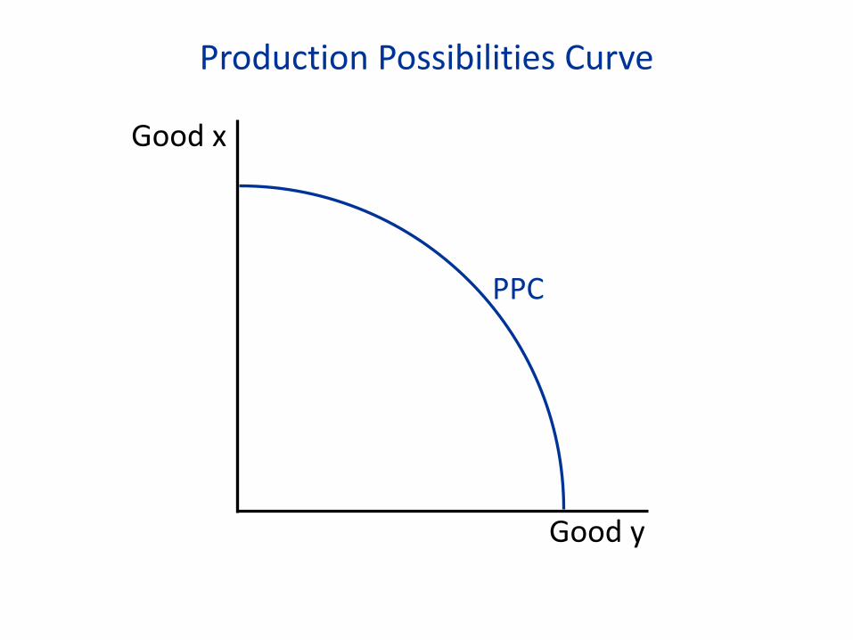
Production Possibilities Curve

PPC

Good y

Good x

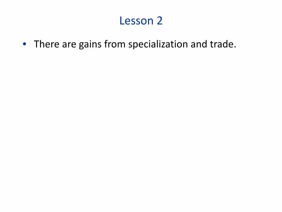
Lesson 2

• There are gains from specialization and trade.

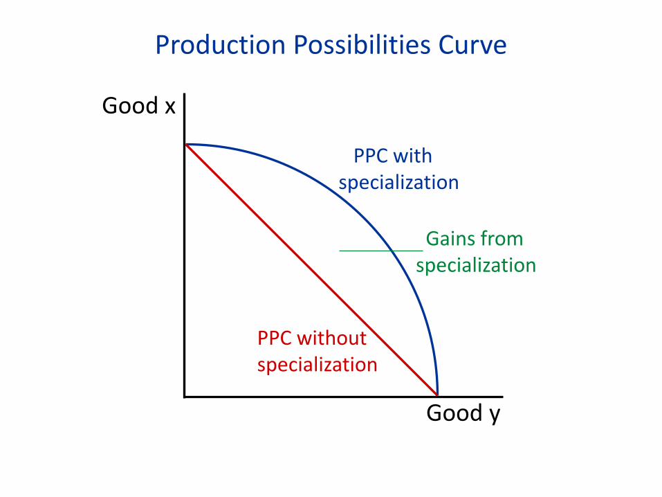
Production Possibilities Curve

PPC with specialization

Good y

Good x

PPC without specialization

Gains from specialization

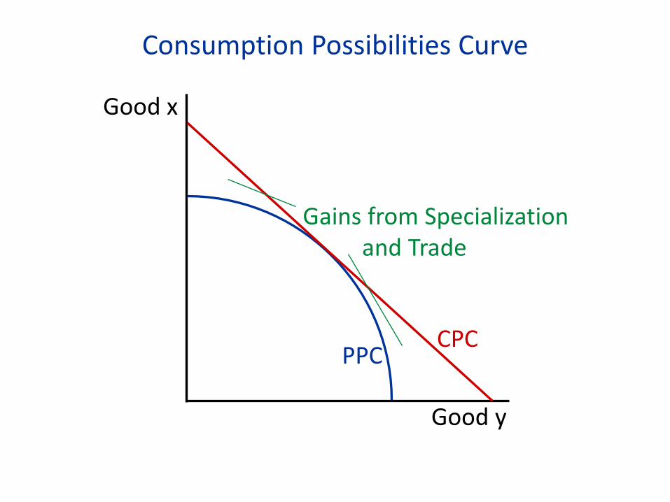
Consumption Possibilities Curve

Good y

PPC

Good x

CPC

Gains from Specialization and Trade

Lesson 3

• In a market system, prices play a crucial role.

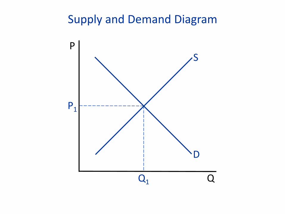
Supply and Demand Diagram

Q

P S

D

P1

Q1

Lesson 4

• Households and firms make choices to maximize their well-being.

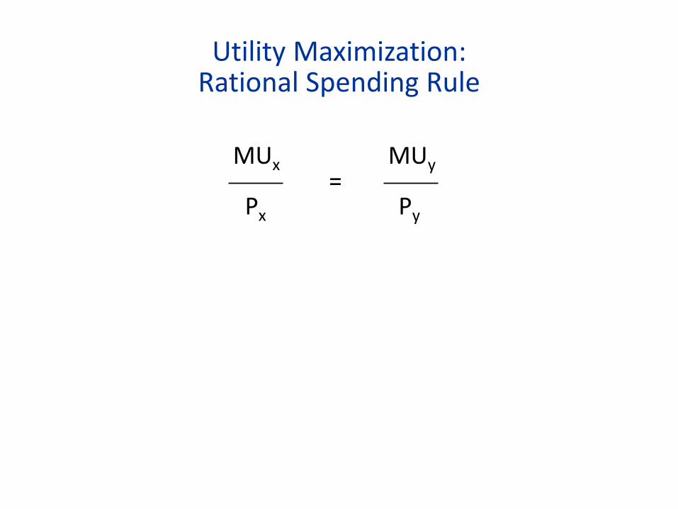
Utility Maximization: Rational Spending Rule

MUx MUy = Px Py

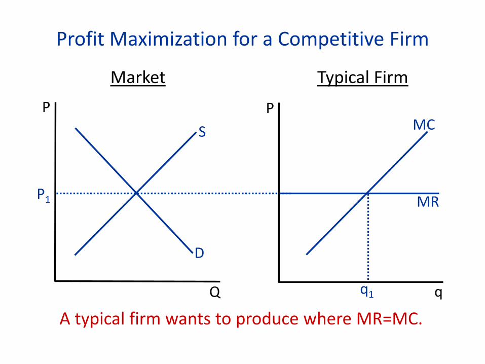
Profit Maximization for a Competitive Firm

q Q

Market

D

S

P1

P P

Typical Firm

MR

MC

q1

A typical firm wants to produce where MR=MC.

Lesson 5

• A market system has many benefits.

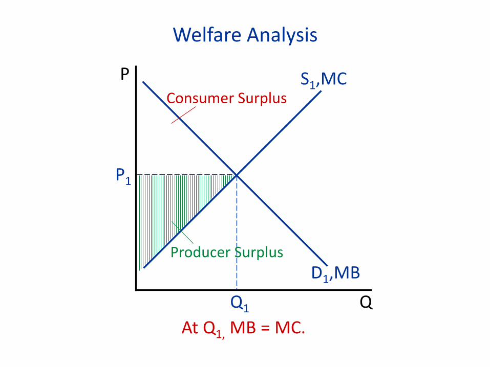
Welfare Analysis

At Q1, MB = MC.

D1,MB Q

P S1,MC

P1

Q1

Producer Surplus

Consumer Surplus

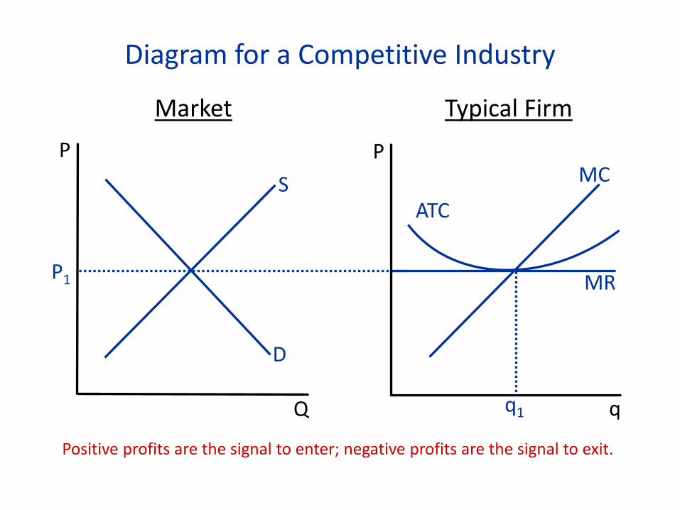
Diagram for a Competitive Industry

q Q

Market

D

S

P1

P P

Typical Firm

MR

MC

q1

ATC

Positive profits are the signal to enter; negative profits are the signal to exit.

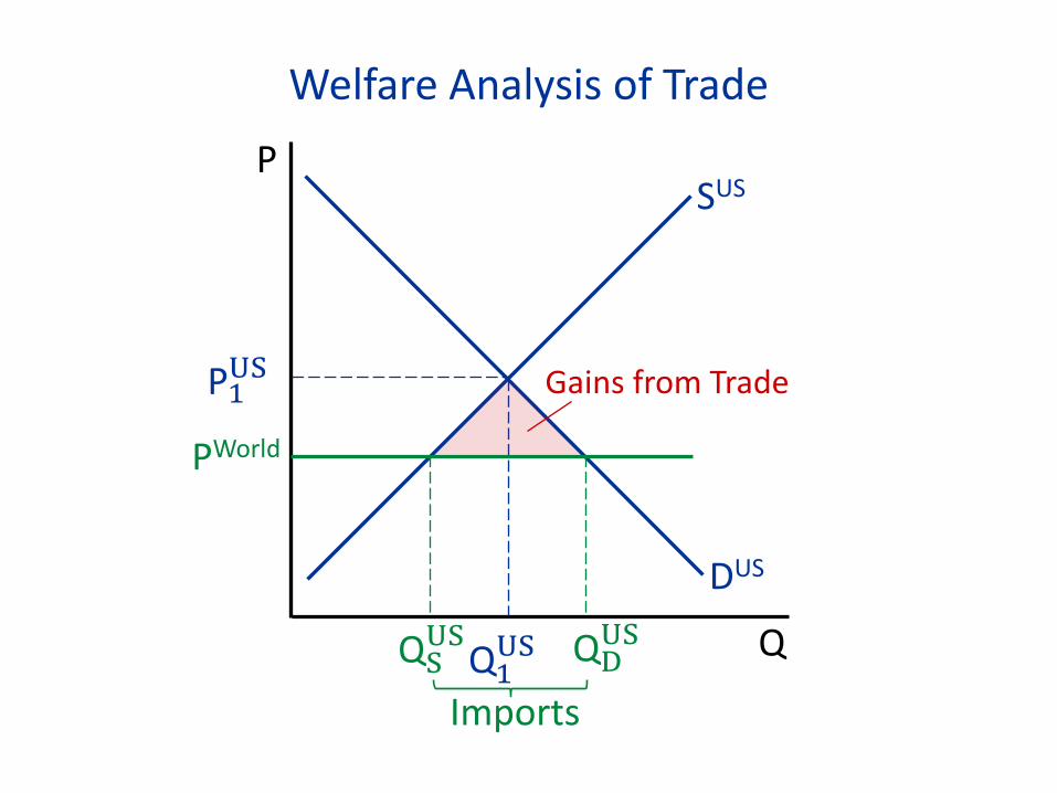
Welfare Analysis of Trade

P1US

Q1US

DUS

Q

P SUS

PWorld

Gains from Trade

QSUS QD

US Imports

Lesson 6

• Interfering with the market has consequences.

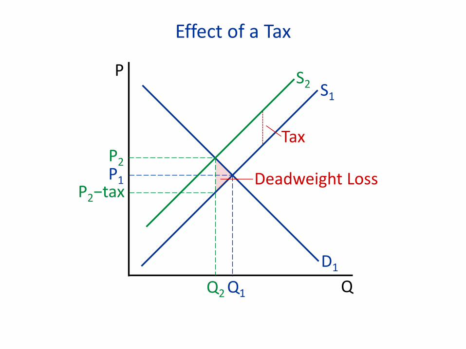
Effect of a Tax

D1 Q

P S1

P1

Q1

S2

Tax

Q2

P2

P2−tax Deadweight Loss

Lesson 7

• Market failures are important, and government interventions can often improve market outcomes.

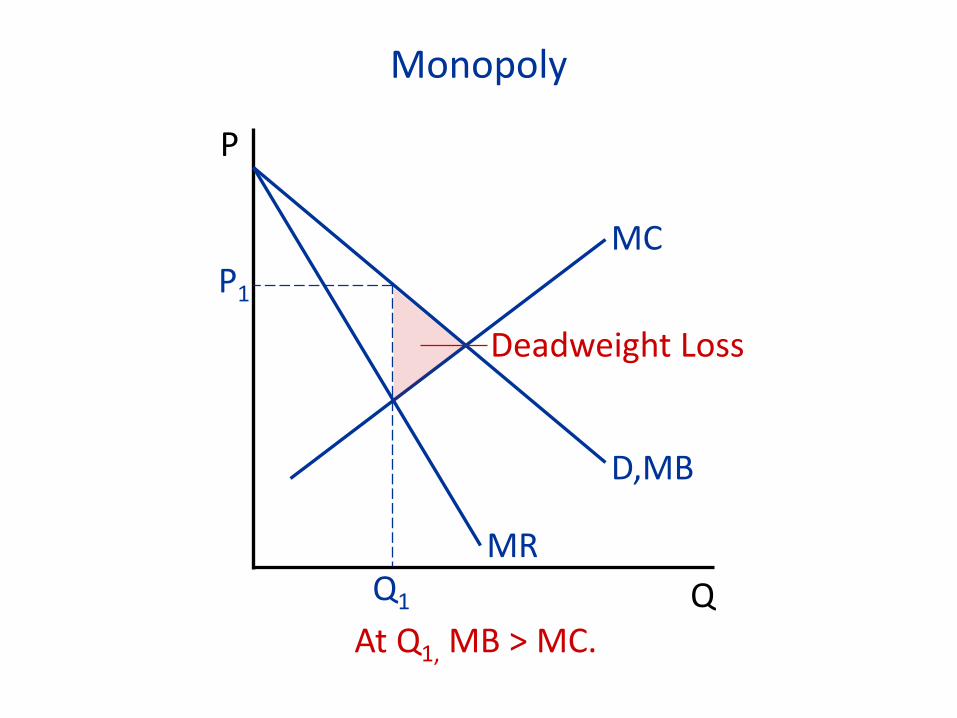
Monopoly

Q

P

D,MB

MR

P1

Q1

MC

Deadweight Loss

At Q1, MB > MC.

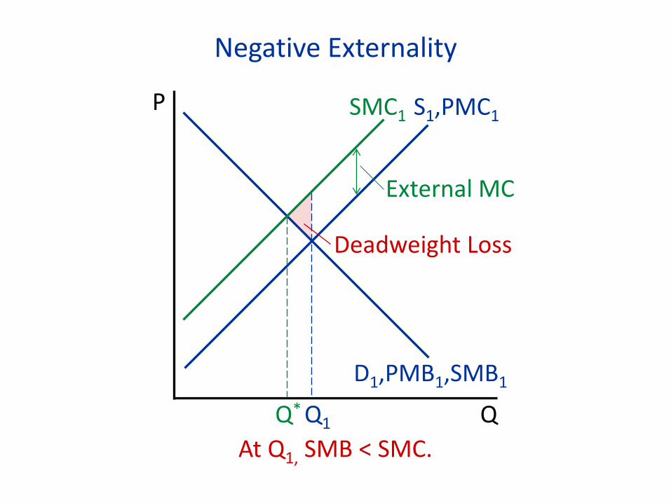
Negative Externality

D1,PMB1,SMB1

Q

P S1,PMC1

Q1

SMC1

Q*

External MC

Deadweight Loss

At Q1, SMB < SMC.

Lesson 8

• Market forces are a fundamental determinant of what workers are paid.

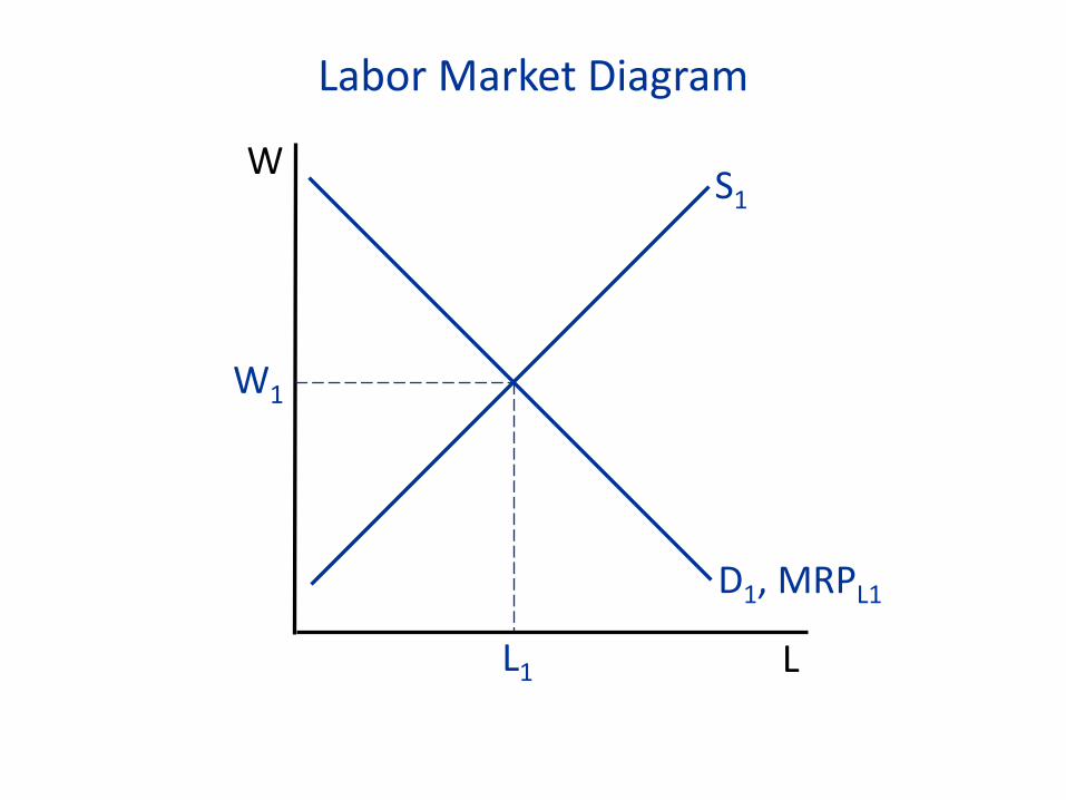
D1, MRPL1

L

W S1

W1

L1

Labor Market Diagram

III. LESSONS AND TOOLS OF MACROECONOMICS

Lesson 1

• In the long run, output is determined by the inputs to the production process.

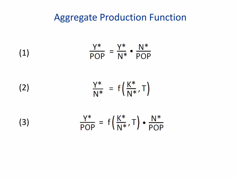
Aggregate Production Function

(1)

(2)

(3) •

Lesson 2

• Improvements in average labor productivity are the key source of economic growth, and technological progress is the key source of improvements in average labor productivity.

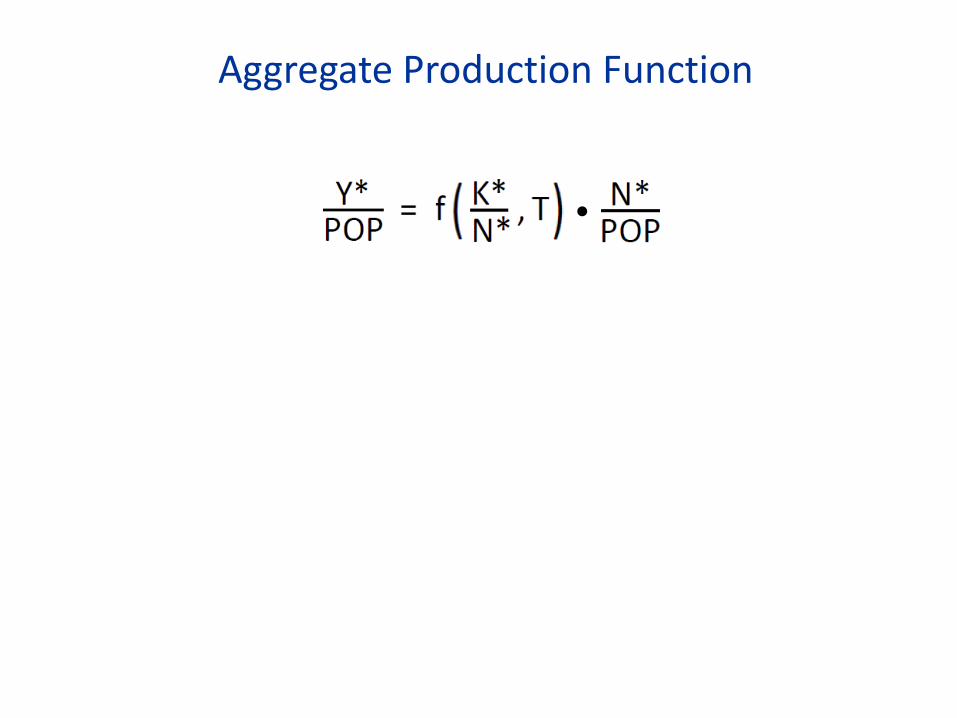
Aggregate Production Function

•

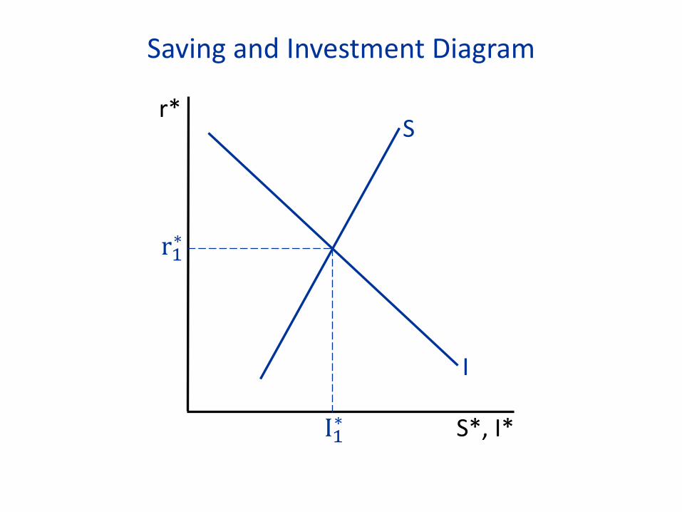
Saving and Investment Diagram

r*

S*, I*

I

r1∗

I1∗

S

Lesson 3

• Changes in planned spending cause output to deviate from potential in the short run.

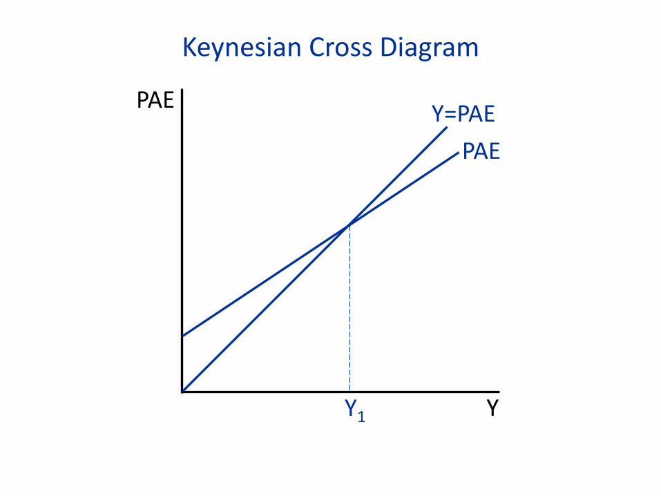
Keynesian Cross Diagram

Y

PAE

PAE Y=PAE

Y1

Lesson 4

• Monetary and fiscal policy affect planned spending, and so can cause or mitigate short-run fluctuations.

Keynesian Cross Diagram

Y

PAE

PAE Y=PAE

Y1

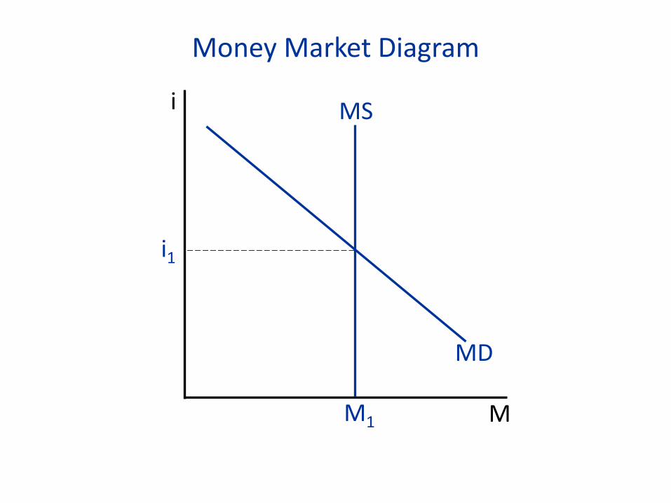
Money Market Diagram

M

i MS

M1

i1

MD

Lesson 5

• Inflation responds gradually to the deviation of output from potential, and this behavior of inflation (working through the Fed’s reaction function) brings the economy back to Y*.

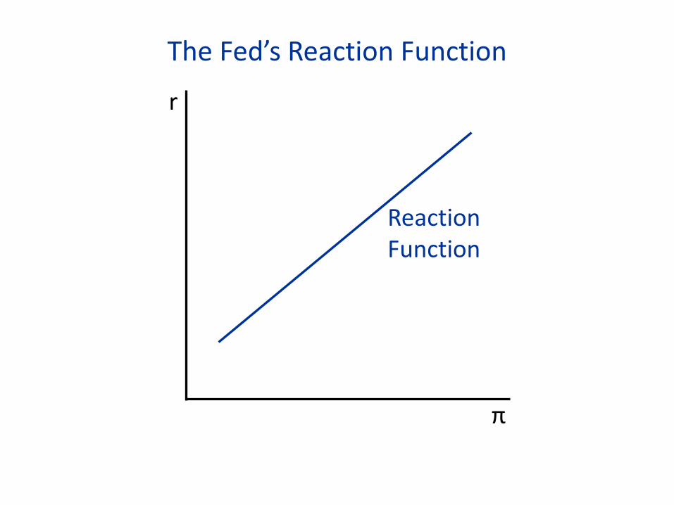
The Fed’s Reaction Function

π

r

Reaction Function

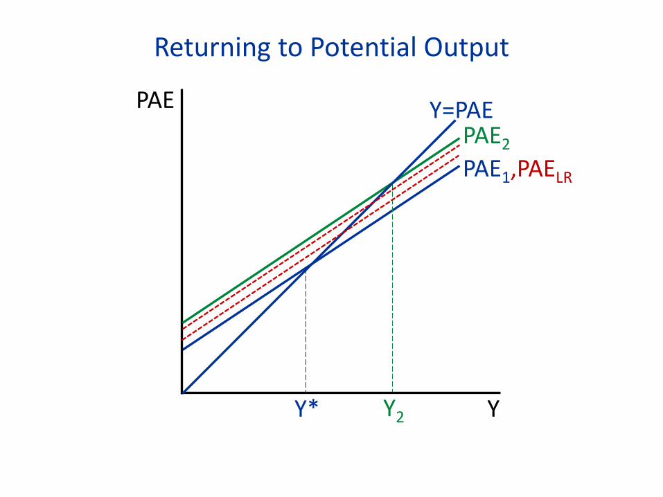
Returning to Potential Output

Y2

PAE2

Y

PAE1,PAELR

PAE Y=PAE

Y*

Lesson 6

• Net exports are determined by factors affecting asset flows, not goods flows.

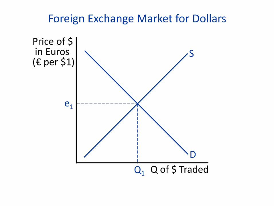
Foreign Exchange Market for Dollars

D Q of $ Traded

S

e1

Q1

Price of $ in Euros (€ per $1)

Balance of Payments

NX + KI = 0